particle imaging velocimetry experiments and lattice ...jos/pbl/phfl14p4012.pdf · acceleration,...

PHYSICS OF FLUIDS VOLUME 14, NUMBER 11 NOVEMBER 2002

Particle imaging velocimetry experiments and lattice-Boltzmannsimulations on a single sphere settling under gravity

A. ten Cate,a) C. H. Nieuwstad, J. J. Derksen, and H. E. A. Van den AkkerKramers Laboratorium voor Fysische Technologie, Delft University of Technology, Prins Bernhardlaan 6,2628 BW Delft, The Netherlands

~Received 26 December 2001; accepted 19 August 2002; published 3 October 2002!

A comparison is made between experiments and simulations on a single sphere settling in silicon oilin a box. Cross-correlation particle imaging velocimetry measurements were carried out at particleReynolds numbers ranging from 1.5 to 31.9. The particle Stokes number varied from 0.2 to 4 andat bottom impact no rebound was observed. Detailed data of the flow field induced by the settlingsphere were obtained, along with time series of the sphere’s trajectory and velocity duringacceleration, steady fall and deceleration at bottom approach. Lattice–Boltzmann simulations proveto capture the full transient behavior of both the sphere motion and the fluid motion. Theexperimental data were used to assess the effect of spatial resolution in the simulations over a rangeof 2–8 grid nodes per sphere radius. The quality of the flow field predictions depends on theReynolds number. When the sphere is very close to the bottom of the container, lubrication theoryhas been applied to compensate for the lack of spatial resolution in the simulations. ©2002American Institute of Physics.@DOI: 10.1063/1.1512918#

nlvamtu

peatesth

reeero

erethmre

sbeu

rene

ererto

id-the

undkesund

on-ar-s-ary

on-heex-hasionslera-hetalset

e

oss

jec-elyod.nu-m-isnalford,of

:

I. INTRODUCTION

Particle motion and particle collisions play an importarole in the performance of many industrial processes invoing suspension flow. For instance, in industrial crystalliztion, crystal–crystal collisions determine kinetic mechanissuch as agglomeration and nucleation due to crystal fracing. Presently, we are developing a method to study sussions under turbulent conditions. For this method, it istempted to fully resolve the flow field around the particland to make a direct coupling between the particle andfluid motion. To validate the way the particles are repsented in the simulation procedure, we compare experimtal and numerical results on the motion of a single sphsettling in a closed box. In the experiment, the transient mtion of a single sphere and its associated flow field wmeasured from the moment of release to a steady-statmaximum settling velocity to deceleration and rest atbottom of the box. For this experiment, the Reynolds nuber, based on the steady-state settling velocity of a sphean infinite medium (Re5r fu`dp /m f) was varied between1.5 and 32. This range of Reynolds numbers was chobecause it corresponds to the range of Reynolds numencountered in our sample crystallization process for prodtion of ammonium sulfate crystals.1

A particle settling towards a wall has been studied pviously by Brenner,2 who derived an analytical solution ithe creeping flow regime. However, at the Reynolds numbstudied, the particle is well out of this regime. Recent expmental work in this field has been presented by sevauthors,3–6 who studied the wall approach and rebound,

a!Telephone: 113-15-2781400; fax:113-15-2782838; electronic [email protected]

4011070-6631/2002/14(11)/4012/14/$19.00

Downloaded 24 Nov 2003 to 128.112.34.89. Redistribution subject to A

t--sr-n--

e-n-e-eor

e-in

enrs

c-

-

rsi-al

obtain restitution coefficients for submerged particles colling with a wall. The parameter that determines rebound isStokes number (St51/9Rerp /r f). Gondretet al.3 demon-strated that the critical Stokes number above which rebooccurs is approximately 10. In our experiments, the Stonumber was varied between 0.19 and 4.13 and no rebowas observed.

We chose to perform the experiment in a closed ctainer for a number of reasons. First, the box width to pticle diameter ratio was kept relatively small, to avoid asumptions regarding the domain size and external boundconditions in the simulations. Thus, the influence of the ctainer walls on the particle motion is contained both in texperiment and in the numerical simulation. Second, theperiment is transient and has a limited time-span. Thisthe advantage that the transient character of the simulatcan be assessed throughout the different stages of accetion, steady fall and deceleration at bottom approach. Tfirst objective of this paper is to present our experimendata on a settling sphere in a confined geometry. The dataconsists of the velocity field of the fluid surrounding thsettling sphere and the trajectory~i.e., position as a functionof time!. The velocity field has been measured using crcorrelation particle image velocimetry7 ~PIV!. The PIV ex-periment is described in the next section. The second obtive is to present our approach to the simulation of fremoving particles based on the lattice-Boltzmann methThis method was chosen because it provides a robustmerical scheme that can efficiently treat the complex geoetry of freely moving particles. A further advantage of thmethod is that it can be parallelized at high computatioefficiency. The use of the lattice-Boltzmann schemesimulation of suspensions has been proposed by Lad8,9

who also presented validation of his method. A number

2 © 2002 American Institute of Physics

IP license or copyright, see http://ojps.aip.org/phf/phfcr.jsp

of

4013Phys. Fluids, Vol. 14, No. 11, November 2002 Particle imaging velocimetry experiments

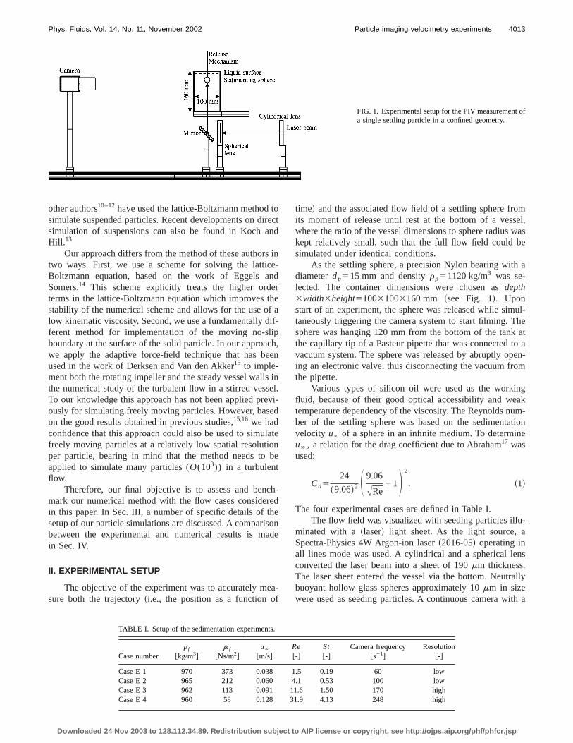
FIG. 1. Experimental setup for the PIV measurementa single settling particle in a confined geometry.

toir

an

s icen

erthf

diflipcee

seeved

laon

b

creheisoad

eaf

omsel,wase

a

ul-heat

to apen-om

gakum-tione

u-a

ns

rally

ith a

other authors10–12have used the lattice-Boltzmann methodsimulate suspended particles. Recent developments on dsimulation of suspensions can also be found in KochHill. 13

Our approach differs from the method of these authortwo ways. First, we use a scheme for solving the lattiBoltzmann equation, based on the work of Eggels aSomers.14 This scheme explicitly treats the higher ordterms in the lattice-Boltzmann equation which improvesstability of the numerical scheme and allows for the use olow kinematic viscosity. Second, we use a fundamentallyferent method for implementation of the moving no-sboundary at the surface of the solid particle. In our approawe apply the adaptive force-field technique that has bused in the work of Derksen and Van den Akker15 to imple-ment both the rotating impeller and the steady vessel wallthe numerical study of the turbulent flow in a stirred vessTo our knowledge this approach has not been applied prously for simulating freely moving particles. However, bason the good results obtained in previous studies,15,16 we hadconfidence that this approach could also be used to simufreely moving particles at a relatively low spatial resolutiper particle, bearing in mind that the method needs toapplied to simulate many particles (O(103)) in a turbulentflow.

Therefore, our final objective is to assess and benmark our numerical method with the flow cases considein this paper. In Sec. III, a number of specific details of tsetup of our particle simulations are discussed. A comparbetween the experimental and numerical results is min Sec. IV.

II. EXPERIMENTAL SETUP

The objective of the experiment was to accurately msure both the trajectory~i.e., the position as a function o


ectd

n-d

ea-

h,n

inl.i-

te

e

h-d

ne

-

time! and the associated flow field of a settling sphere frits moment of release until rest at the bottom of a veswhere the ratio of the vessel dimensions to sphere radiuskept relatively small, such that the full flow field could bsimulated under identical conditions.

As the settling sphere, a precision Nylon bearing withdiameterdp515 mm and densityrp51120 kg/m3 was se-lected. The container dimensions were chosen asdepth3width3height510031003160 mm ~see Fig. 1!. Uponstart of an experiment, the sphere was released while simtaneously triggering the camera system to start filming. Tsphere was hanging 120 mm from the bottom of the tankthe capillary tip of a Pasteur pipette that was connectedvacuum system. The sphere was released by abruptly oing an electronic valve, thus disconnecting the vacuum frthe pipette.

Various types of silicon oil were used as the workinfluid, because of their good optical accessibility and wetemperature dependency of the viscosity. The Reynolds nber of the settling sphere was based on the sedimentavelocity u` of a sphere in an infinite medium. To determinu` , a relation for the drag coefficient due to Abraham17 wasused:

Cd524

~9.06!2 S 9.06

ARe11D 2

. ~1!

The four experimental cases are defined in Table I.The flow field was visualized with seeding particles ill

minated with a~laser! light sheet. As the light source,Spectra-Physics 4W Argon-ion laser~2016-05! operating inall lines mode was used. A cylindrical and a spherical leconverted the laser beam into a sheet of 190mm thickness.The laser sheet entered the vessel via the bottom. Neutbuoyant hollow glass spheres approximately 10mm in sizewere used as seeding particles. A continuous camera w

TABLE I. Setup of the sedimentation experiments.

Case numberr f

@kg/m3#m f

@Ns/m2#u`

@m/s#Re@-#

St@-#

Camera frequency@s21#

Resolution@-#

Case E 1 970 373 0.038 1.5 0.19 60 lowCase E 2 965 212 0.060 4.1 0.53 100 lowCase E 3 962 113 0.091 11.6 1.50 170 highCase E 4 960 58 0.128 31.9 4.13 248 high


12o

diti

ea

t o

bae

umwaAnhenggh3

ts.am

r

lu

rra-me,r aeetingthedasKu--ats

s

aheere

athoxi-entssti-

0.5ci-ar-

thepu-talue

eoutri-

een.pa-

ure-ell.

4014 Phys. Fluids, Vol. 14, No. 11, November 2002 ten Cate et al.

frame rate up to 250 Hz and an array size of 53512 pixels was used to record the experiment. The flfield was measured on a grid of interrogation areas~IA’s !. AnIA typically contained 32332 pixels. The fluid velocity wasdetermined in each interrogation area by estimating theplacement of the seeding particles between two consecuframes through cross correlation.18

The desired spatial resolution and the maximum camframe rate set a restriction to the maximum fluid velocity thcan be accurately measured, as between two framestracer particles are not allowed to shift more than 1/4 parthe linear size of an interrogation area.7 This limits the maxi-mum sedimentation velocity of the sphere, which cantaken as a measure for the maximum fluid velocity duringexperiment. The required resolution depends on the Rnolds number of the flow, because at higher Reynolds nbers, the structures in the flow become smaller. The flowmeasured at either of the two resolutions given in Fig. 2.the low resolution@Fig. 2~b!#, when the array size is choseto map three sphere diameters, the maximum allowed spvelocity is 0.18 m/s, which is larger than any of the settlivelocities of the Nylon sphere as given in Table I. At the hiresolution@Fig. 2~a!#, the maximum allowed velocity is 0.1m/s, which is close to the sedimentation velocity of caseE4.However, the sphere is expected to move at a velocity thalower thanu` due to hindrance from the container wallBased on the 1/4 part displacement rule, the camera frrate was adjusted for each experiment.

To capture the full trajectory of the particle, three ovelapping fields of view~FOV! were used at low resolution~casesE1 andE2) while the measurements at high resotion ~casesE3 andE4) were done in four FOV’s~see Fig.

FIG. 2. Measurement positions at high~a! and low ~b! resolution.


w

s-ve

ratthef

eny--st

re

is

e

-

-

2!. A raw image is given in Fig. 3~a!. As can be seen, theleading side of the sphere was made dark to prevent ovediation due to reflections at the sphere surface. In each frathe sphere position had to be determined accurately fogood interpretation of the flow field. Because the laser shenters from the bottom and is blocked by the sedimentsphere, no fluid velocities could be measured behindsphere@Fig. 4~a!#. The sphere’s position was determinefrom the colored top of the sphere. The motion blur wremoved from the sphere by using an edge-preservingwahara filter19 @Fig. 3~b!# and after having applied a threshold @Fig. 3~c!#, they position of the sphere was determinedpixel accuracy@Fig. 3~d!#. The resulting sphere trajectorieand velocities are given in Fig. 5.

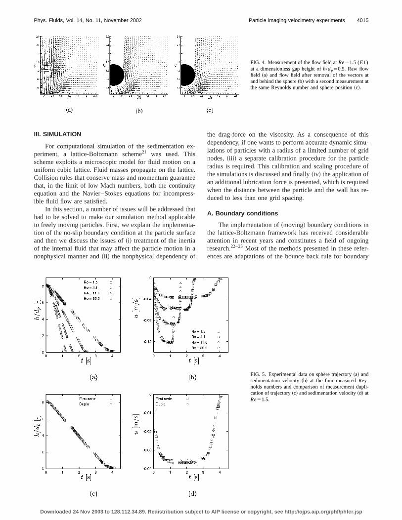
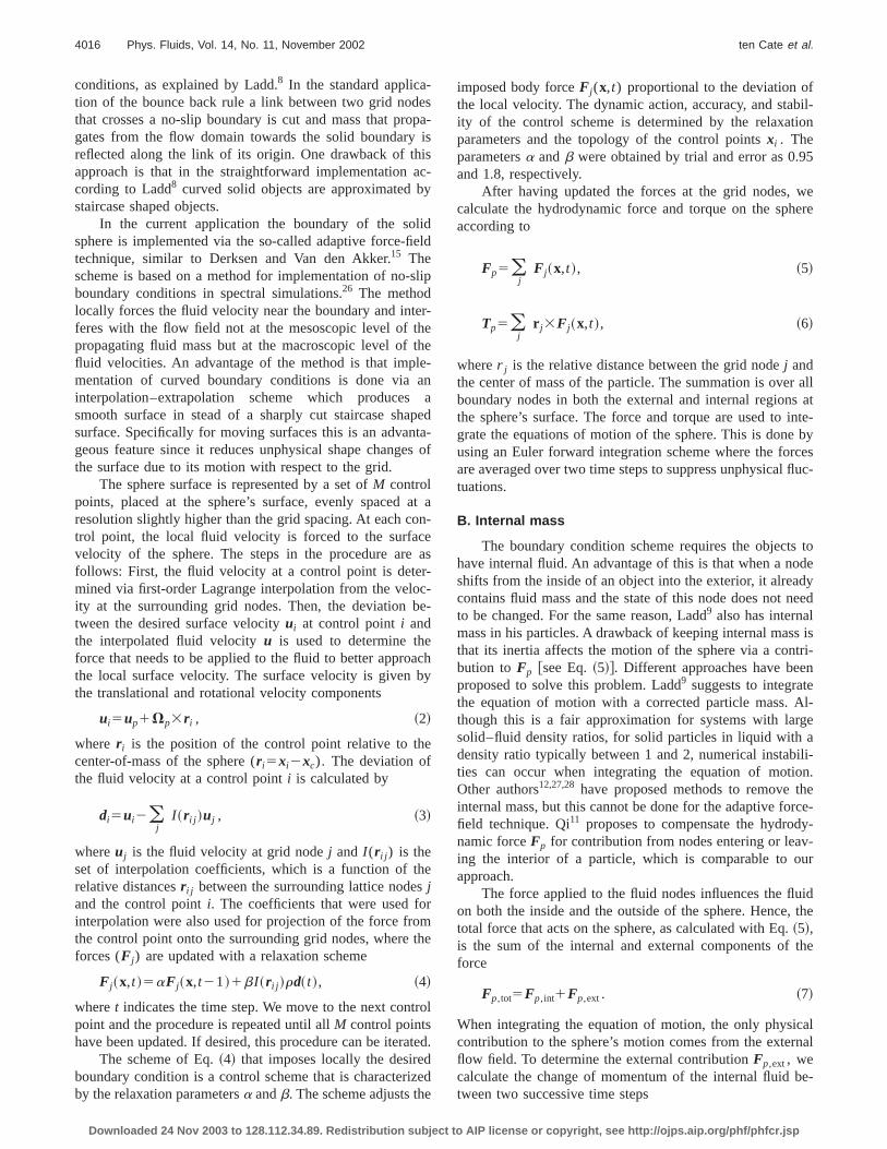
A raw vector image of the flow at a particle Reynoldnumber of 1.5 is given in Fig. 4~a!. Interrogation was donewith IA’s of 32332 pixels with a 50% overlap, resulting intotal of 961 vectors per image. After determination of tsphere position, the vectors inside and behind the sphwere removed from the image and~for reference! a spherewas placed in the figure, as can be seen in Fig. 4~b!. In thisfigure, the maximum velocities are found closely undernethe sphere where tracer particle displacements of apprmately 7 pixels were found. Velocities far away from thsphere become very low, which gives particle displacemesmaller than 0.5 pixel. Sub-pixel displacements were emated using a Gaussian peak fit estimator.18 The accuracy isapproximately 0.1 pixel for displacements larger thanpixel, leading to a relative error of 2% for the highest veloties, whereas the relative error is approximately 17% for pticle displacements less than 0.5 pixel. After removal ofvectors inside and behind the sphere, approximately 10 srious vectors remain per frame. This is about 1% of the toamount of vectors which is low compared to a typical valof 5% encountered in turbulent flow fields.20 This is due tothe flow being laminar and virtually two-dimensional in thcenter plane of the sphere, which results in practically noof plane motion. To test the reproducibility of the expement, all measurements were done twice. In Figs. 5~c! and5~d!, the trajectories and sedimentation velocities have bplotted for caseE1. The two trajectories practically coincideThe measurements at higher Reynolds numbers give comrable results. The flow fields around the sphere of caseE1are presented in Fig. 4 to demonstrate that the PIV measments yields an accurately reproducible result here as w

on.
FIG. 3. Processing steps in detection of sphere positi~a! Raw PIV-recording with sphere.~b! Part of record-ing after a Kuwahara-filter has been applied.~c! Resultof thresholding image~b!. ~d! Magnification of the rearside of the sphere.

tt


FIG. 4. Measurement of the flow field atRe51.5 (E1)at a dimensionless gap height ofh/dp50.5. Raw flowfield ~a! and flow field after removal of the vectors aand behind the sphere~b! with a second measurement athe same Reynolds number and sphere position~c!.

x

aicnttyes

thbtac

af

thismu-idcle

of

redre-

bleinger-dary

III. SIMULATION

For computational simulation of the sedimentation eperiment, a lattice-Boltzmann scheme21 was used. Thisscheme exploits a microscopic model for fluid motion onuniform cubic lattice. Fluid masses propagate on the lattCollision rules that conserve mass and momentum guarathat, in the limit of low Mach numbers, both the continuiequation and the Navier–Stokes equations for incomprible fluid flow are satisfied.

In this section, a number of issues will be addressedhad to be solved to make our simulation method applicato freely moving particles. First, we explain the implemention of the no-slip boundary condition at the particle surfaand then we discuss the issues of~i! treatment of the inertiaof the internal fluid that may affect the particle motion innonphysical manner and~ii ! the nonphysical dependency o


-

e.ee

s-

atle-e

the drag-force on the viscosity. As a consequence ofdependency, if one wants to perform accurate dynamic silations of particles with a radius of a limited number of grnodes,~iii ! a separate calibration procedure for the partiradius is required. This calibration and scaling procedurethe simulations is discussed and finally~iv! the application ofan additional lubrication force is presented, which is requiwhen the distance between the particle and the wall hasduced to less than one grid spacing.

A. Boundary conditions

The implementation of~moving! boundary conditions inthe lattice-Boltzmann framework has received consideraattention in recent years and constitutes a field of ongoresearch.22–25 Most of the methods presented in these refences are adaptations of the bounce back rule for boun

-pli-

FIG. 5. Experimental data on sphere trajectory~a! andsedimentation velocity~b! at the four measured Reynolds numbers and comparison of measurement ducation of trajectory~c! and sedimentation velocity~d! atRe51.5.


-e

opi

isacby

lide

sl

erhethlea

pta

es

ane

r-c

be

eacby

e

esrmth

ro

atdizee

fbil-ion

5

weere

alls atinte-by

cesfluc-

tode

dyeed

s istri-n

Al-geaili-n.

herce-y--ur

id, the

the

alnal

be-


conditions, as explained by Ladd.8 In the standard application of the bounce back rule a link between two grid nodthat crosses a no-slip boundary is cut and mass that prgates from the flow domain towards the solid boundaryreflected along the link of its origin. One drawback of thapproach is that in the straightforward implementationcording to Ladd8 curved solid objects are approximatedstaircase shaped objects.

In the current application the boundary of the sosphere is implemented via the so-called adaptive force-fitechnique, similar to Derksen and Van den Akker.15 Thescheme is based on a method for implementation of no-boundary conditions in spectral simulations.26 The methodlocally forces the fluid velocity near the boundary and intferes with the flow field not at the mesoscopic level of tpropagating fluid mass but at the macroscopic level offluid velocities. An advantage of the method is that impmentation of curved boundary conditions is done viainterpolation–extrapolation scheme which producessmooth surface in stead of a sharply cut staircase shasurface. Specifically for moving surfaces this is an advangeous feature since it reduces unphysical shape changthe surface due to its motion with respect to the grid.

The sphere surface is represented by a set ofM controlpoints, placed at the sphere’s surface, evenly spacedresolution slightly higher than the grid spacing. At each cotrol point, the local fluid velocity is forced to the surfacvelocity of the sphere. The steps in the procedure arefollows: First, the fluid velocity at a control point is detemined via first-order Lagrange interpolation from the veloity at the surrounding grid nodes. Then, the deviationtween the desired surface velocityui at control pointi andthe interpolated fluid velocityu is used to determine thforce that needs to be applied to the fluid to better approthe local surface velocity. The surface velocity is giventhe translational and rotational velocity components

ui5up1Vp3r i , ~2!

where r i is the position of the control point relative to thcenter-of-mass of the sphere (r i5xi2xc). The deviation ofthe fluid velocity at a control pointi is calculated by

di5ui2(j

I ~r i j !uj , ~3!

whereuj is the fluid velocity at grid nodej and I (r i j ) is theset of interpolation coefficients, which is a function of threlative distancesr i j between the surrounding lattice nodejand the control pointi. The coefficients that were used fointerpolation were also used for projection of the force frothe control point onto the surrounding grid nodes, whereforces (F j ) are updated with a relaxation scheme

F j~x,t !5aF j~x,t21!1bI ~r i j !rd~ t !, ~4!

wheret indicates the time step. We move to the next contpoint and the procedure is repeated until allM control pointshave been updated. If desired, this procedure can be iter

The scheme of Eq.~4! that imposes locally the desireboundary condition is a control scheme that is characterby the relaxation parametersa andb. The scheme adjusts th


sa-

s

-

ld

ip

-

e-naed-of

t a-

as

--

h

e

l

ed.

d

imposed body forceF j (x,t) proportional to the deviation othe local velocity. The dynamic action, accuracy, and staity of the control scheme is determined by the relaxatparameters and the topology of the control pointsxi . Theparametersa andb were obtained by trial and error as 0.9and 1.8, respectively.

After having updated the forces at the grid nodes,calculate the hydrodynamic force and torque on the sphaccording to

Fp5(j

F j~x,t !, ~5!

Tp5(j

r j3F j~x,t !, ~6!

wherer j is the relative distance between the grid nodej andthe center of mass of the particle. The summation is overboundary nodes in both the external and internal regionthe sphere’s surface. The force and torque are used tograte the equations of motion of the sphere. This is doneusing an Euler forward integration scheme where the forare averaged over two time steps to suppress unphysicaltuations.

B. Internal mass

The boundary condition scheme requires the objectshave internal fluid. An advantage of this is that when a noshifts from the inside of an object into the exterior, it alreacontains fluid mass and the state of this node does not nto be changed. For the same reason, Ladd9 also has internalmass in his particles. A drawback of keeping internal masthat its inertia affects the motion of the sphere via a conbution to Fp @see Eq.~5!#. Different approaches have beeproposed to solve this problem. Ladd9 suggests to integratethe equation of motion with a corrected particle mass.though this is a fair approximation for systems with larsolid–fluid density ratios, for solid particles in liquid withdensity ratio typically between 1 and 2, numerical instabties can occur when integrating the equation of motioOther authors12,27,28 have proposed methods to remove tinternal mass, but this cannot be done for the adaptive fofield technique. Qi11 proposes to compensate the hydrodnamic forceFp for contribution from nodes entering or leaving the interior of a particle, which is comparable to oapproach.

The force applied to the fluid nodes influences the fluon both the inside and the outside of the sphere. Hencetotal force that acts on the sphere, as calculated with Eq.~5!,is the sum of the internal and external components offorce

Fp,tot5Fp, int1Fp,ext. ~7!

When integrating the equation of motion, the only physiccontribution to the sphere’s motion comes from the exterflow field. To determine the external contributionFp,ext, wecalculate the change of momentum of the internal fluidtween two successive time steps


icowio

-nre

byarru

io-slitythoa

sopoeh

tht

-

-elyan

o

ityasr

caerc

vellrT

ra-thengleontheldsu-

x-be

nd. Atarilyalgthali-isfor

wreedto

en-ro-os-ndhe.

attheul-

thehis

s,

ional

thehri-


F~ t !p, int5E E EVsphere

ruint~x,t !2ruint~x,t21!dV, ~8!

and subtract this from the total forceFp,tot . When using thisapproach the correct physical behavior is obtained, whallows us to simulate particle motion at a density ratio as las 1.15, as is demonstrated in Sec. IV. A similar correctprocedure is applied for the torque.

C. Low Reynolds number calibration

Results presented by Ladd9 indicated that boundary conditions in lattice-Boltzmann schemes based on the bouback rule suffer from a nonphysical dependency of thesulting drag force on the kinematic viscosity. A studyRohdeet al.25 indicated that also more advanced boundcondition methods that are based on the bounce backstill exhibit this behavior. A detailed analysis of this behavis given by He et al.,29 who demonstrate that in latticeBoltzmann methods, the exact position at which the no-condition is obtained is a function of the kinematic viscosiAlthough there is a fundamental difference betweenbounce back boundary condition and our approach, this nphysical dependency is also observed in our currentproach.

An explanation for the fact that this behavior is alobserved in our simulations may be that due to the interlation and extrapolation procedure, the sphere’s surfacsmeared out and the fluid experiences a sphere that is sligbigger than the sphere on which theM control points lie. Theresult of this effect is that the drag force obtained fromsimulation is larger than the force that would correspondthe sphere’s given input radius.

To compensate for this effect, Ladd9 proposed a procedure for estimating the effective sphere radius~hereaftercalledhydrodynamic radius!. Ladd demonstrated that the hydrodynamic radius varied with viscosity as approximatone grid node. The calibration procedure is based on anlytic expression of Hasimoto30 for the drag force on a fixedsphere in a periodic array of spheres in the creeping flregime

6pmr pUv

Fp51.021.7601Ct

1/31Ct21.5593Ct2,

Ct54pr p

3

3L3 , ~9!

wherer p is the sphere radius,L indicates the size of the uncell, and Uv is the volumetrically averaged fluid velocitacross the periodic cell. For a given fluid velocity and drforce, Eq.~9! is solved to calculate the hydrodynamic radiu

In our simulations we use a similar calibration proceduas proposed by Ladd. We want to stress here that thisbration procedure is performed independent of the expmental conditions or results. The sole purpose of this produre is to determined the equivalent particle diameter, gia certain viscosity. A sphere is placed in the center of a fuperiodic cell and the fluid is set into motion via a pressugradient, such that the Reynolds number remains small.


h

n

ce-

yle

r

p.en-p-

-istly

eo

a-

w

g.eli-i-e-nyehe

hydrodynamic radius is determined as the average of thedius at 20 sphere positions, which were taken parallel toflow because the settling sphere also moves along a siaxis. One can ask if this low Reynolds number calibratiprocedure is allowed when it is our objective to simulatetransient motion of a sphere moving at nonzero Reynonumbers. Therefore, in Sec. IV D the sensitivity of the simlations to the hydrodynamic radius is investigated.

D. Scaling

When setting up a simulation of the sedimentation eperiment, the scaling of mass, length, and time needs todetermined. With respect to mass, only the ratio of fluid asolid density enters the equations of motion of the systema constant ratio, the actual values can be chosen arbitrwithout influencing the simulation result. Their numericvalues were set identical to the experimental values. Lenand time are scaled by using the low Reynolds number cbration procedure. A first estimate for the length scalebased on the input radius of the sphere. A first estimatethe time scale is then determined by settingu` to 0.01lu/ts@in lattice-Boltzmann simulations,umax!cs ~the speed ofsound,cs5

12&) is required to assure incompressible flo

conditions#. With these first estimates, all parameters ascaled from the physical experiment into lattice units. Bason this first scaling, a calibration simulation is carried outdetermine the hydrodynamic radius. Finally, in the sedimtation simulations, length is scaled on the basis of the hyddynamic radius and time is scaled via the kinematic viscity. In Sec. IV, calibration results of input radii between 2 a8 lattice units will be presented, and the sensitivity of tsimulations to the hydrodynamic radius will be discussed

E. Sub-grid lubrication force

When simulating a sphere approaching a fixed wall,some moment in time the grid lacks resolution to resolveflow in the gap between the sphere and the wall. The repsive forces that occur due to the squeezing motion offluid in the gap can no longer be computed accurately. Tproblem was noticed by Ladd,31 who proposed to include anexplicit expression for the leading order lubrication forcecalculated with lubrication theory.32,33 In our simulations,when the gap has become smaller thanD0 ~set to 1 gridspacing!, the force acting on the sphere due to the lubricatin the unresolved gap is calculated explicitly. The additionlubrication force at gap distanceh is calculated with

Fw526pmr pu'S r p

h2

r p

D0D , ~10!

whereh is the gap between the wall and the sphere andu' isthe velocity component of the sphere perpendicular towall. In the following section, the validity of this approacwill be tested by comparing simulation results with expemental data.


ius of

icalxperi-


Downloaded 24 N

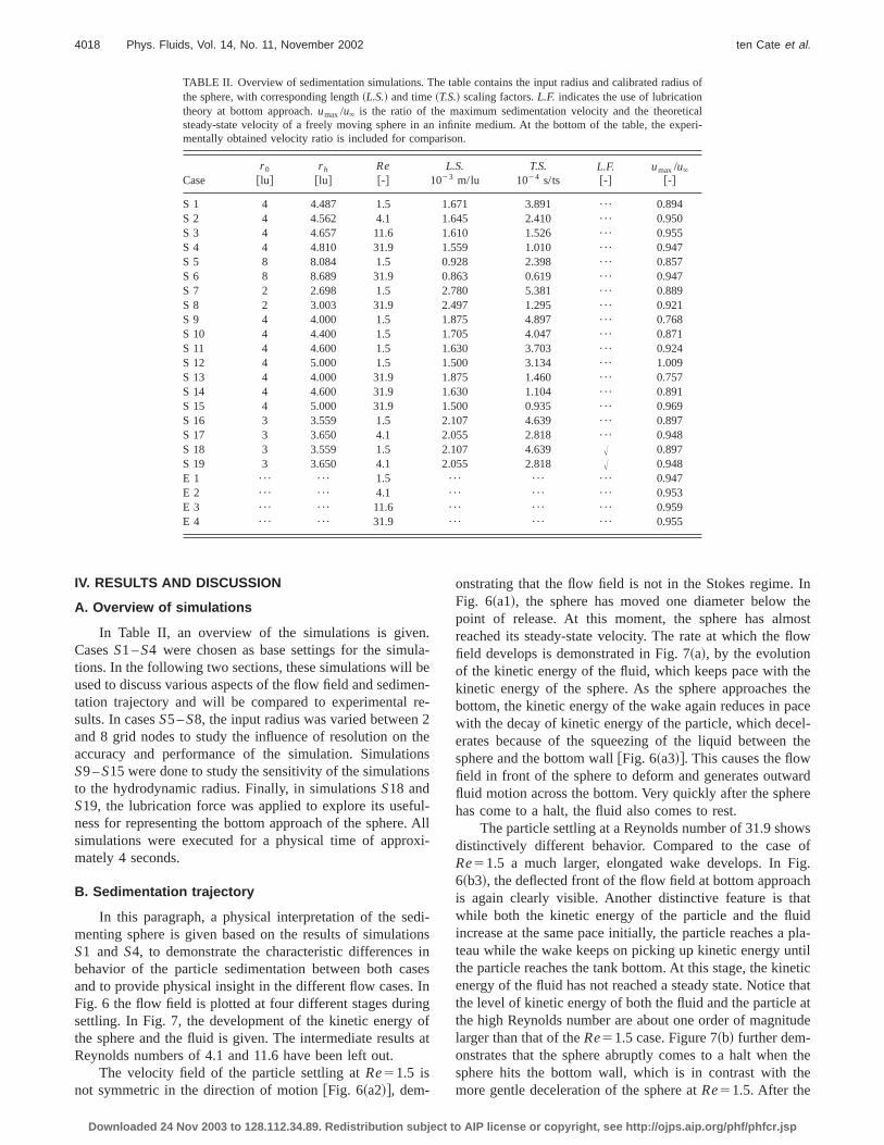
TABLE II. Overview of sedimentation simulations. The table contains the input radius and calibrated radthe sphere, with corresponding length~L.S.! and time~T.S.! scaling factors.L.F. indicates the use of lubricationtheory at bottom approach.umax/u` is the ratio of the maximum sedimentation velocity and the theoretsteady-state velocity of a freely moving sphere in an infinite medium. At the bottom of the table, the ementally obtained velocity ratio is included for comparison.

Caser 0

@lu#r h

@lu#Re@-#

L.S.1023 m/lu

T.S.1024 s/ts

L.F.@-#

umax/u`

@-#

S 1 4 4.487 1.5 1.671 3.891 ¯ 0.894S 2 4 4.562 4.1 1.645 2.410 ¯ 0.950S 3 4 4.657 11.6 1.610 1.526 ¯ 0.955S 4 4 4.810 31.9 1.559 1.010 ¯ 0.947S 5 8 8.084 1.5 0.928 2.398 ¯ 0.857S 6 8 8.689 31.9 0.863 0.619 ¯ 0.947S 7 2 2.698 1.5 2.780 5.381 ¯ 0.889S 8 2 3.003 31.9 2.497 1.295 ¯ 0.921S 9 4 4.000 1.5 1.875 4.897 ¯ 0.768S 10 4 4.400 1.5 1.705 4.047 ¯ 0.871S 11 4 4.600 1.5 1.630 3.703 ¯ 0.924S 12 4 5.000 1.5 1.500 3.134 ¯ 1.009S 13 4 4.000 31.9 1.875 1.460 ¯ 0.757S 14 4 4.600 31.9 1.630 1.104 ¯ 0.891S 15 4 5.000 31.9 1.500 0.935 ¯ 0.969S 16 3 3.559 1.5 2.107 4.639 ¯ 0.897S 17 3 3.650 4.1 2.055 2.818 ¯ 0.948S 18 3 3.559 1.5 2.107 4.639 A 0.897S 19 3 3.650 4.1 2.055 2.818 A 0.948E 1 ¯ ¯ 1.5 ¯ ¯ ¯ 0.947E 2 ¯ ¯ 4.1 ¯ ¯ ¯ 0.953E 3 ¯ ¯ 11.6 ¯ ¯ ¯ 0.959E 4 ¯ ¯ 31.9 ¯ ¯ ¯ 0.955

n.la

bee

re2

thnn

ul. Axi

dio

isIn

ngos

Intheostow

hethe

aceel-the

ardre

wsofig.chatidpla-

ntileticthatatude

thehe

IV. RESULTS AND DISCUSSION

A. Overview of simulations

In Table II, an overview of the simulations is giveCasesS1 –S4 were chosen as base settings for the simutions. In the following two sections, these simulations willused to discuss various aspects of the flow field and sedimtation trajectory and will be compared to experimentalsults. In casesS5 –S8, the input radius was varied betweenand 8 grid nodes to study the influence of resolution onaccuracy and performance of the simulation. SimulatioS9 –S15 were done to study the sensitivity of the simulatioto the hydrodynamic radius. Finally, in simulationsS18 andS19, the lubrication force was applied to explore its usefness for representing the bottom approach of the spheresimulations were executed for a physical time of appromately 4 seconds.

B. Sedimentation trajectory

In this paragraph, a physical interpretation of the sementing sphere is given based on the results of simulatS1 andS4, to demonstrate the characteristic differencesbehavior of the particle sedimentation between both caand to provide physical insight in the different flow cases.Fig. 6 the flow field is plotted at four different stages durisettling. In Fig. 7, the development of the kinetic energythe sphere and the fluid is given. The intermediate resultReynolds numbers of 4.1 and 11.6 have been left out.

The velocity field of the particle settling atRe51.5 isnot symmetric in the direction of motion@Fig. 6~a2!#, dem-

ov 2003 to 128.112.34.89. Redistribution subject to A

-

n--

ess

-ll

-

i-nsnes

fat

onstrating that the flow field is not in the Stokes regime.Fig. 6~a1!, the sphere has moved one diameter belowpoint of release. At this moment, the sphere has almreached its steady-state velocity. The rate at which the flfield develops is demonstrated in Fig. 7~a!, by the evolutionof the kinetic energy of the fluid, which keeps pace with tkinetic energy of the sphere. As the sphere approachesbottom, the kinetic energy of the wake again reduces in pwith the decay of kinetic energy of the particle, which decerates because of the squeezing of the liquid betweensphere and the bottom wall@Fig. 6~a3!#. This causes the flowfield in front of the sphere to deform and generates outwfluid motion across the bottom. Very quickly after the sphehas come to a halt, the fluid also comes to rest.

The particle settling at a Reynolds number of 31.9 shodistinctively different behavior. Compared to the caseRe51.5 a much larger, elongated wake develops. In F6~b3!, the deflected front of the flow field at bottom approais again clearly visible. Another distinctive feature is thwhile both the kinetic energy of the particle and the fluincrease at the same pace initially, the particle reaches ateau while the wake keeps on picking up kinetic energy uthe particle reaches the tank bottom. At this stage, the kinenergy of the fluid has not reached a steady state. Noticethe level of kinetic energy of both the fluid and the particlethe high Reynolds number are about one order of magnitlarger than that of theRe51.5 case. Figure 7~b! further dem-onstrates that the sphere abruptly comes to a halt whensphere hits the bottom wall, which is in contrast with tmore gentle deceleration of the sphere atRe51.5. After the


exll,


FIG. 6. Comparison of the flow fieldof the sedimenting sphere at~a!, Re51.5 ~top, case S1) and ~b!, Re531.9 ~bottom, caseS4). The con-tours indicate the normalized velocitymagnitude.h/dp indicates the dimen-sionless gap between the bottom apof the sphere and the tank bottom wat indicates time.

smat

tichengyhe

e

or

there.

ar-le is

anion-m-en-

wthe

etime

sphere has come to a halt, the wake still contains a conerable amount of kinetic energy that slowly decays. An epirical time constant related to this process can be estimby assuming an exponential function

K f~ t !5K f ,maxexpS 2t

tdD , ~11!

which is plotted in Fig. 7~b! with td50.3@s#.A remark can be made on the distribution of the kine

energy over the particle and the fluid. During settling tpotential energy of the particle is transferred to the fluid adissipated. At maximum settling velocity, the kinetic enerof the fluid is much larger than that of the particle. Tvolume of the moving fluid is much larger than the volumof the particle~see also Fig. 6! and since the solid–liquiddensity ratio is small, the fluid can easily contain much mkinetic energy than the particle.


id--ed

d

e

Three physical time scales can be used to interpretflow field and transient behavior of the sedimenting spheThe first time scale is the particle advection time (tp,a

.dp /u`), which is a measure for the time it takes the pticle to travel one sphere diameter. The second time scathe particle relaxation time, (tp,r.rpdp

2/18r fn) which is ameasure for the time it takes for a particle to respond toacceleration. The third time scale is the momentum diffustime (tn.dp

2/n), which is a measure for diffusion of momentum into the fluid over a distance of one particle diaeter. These three groups determine two independent dimsionless numbers, the Reynolds and Stokes number.

The different shapes of the flow field in the high and loReynolds number cases can be interpreted by regardingReynolds numbers as the ratio oftn and tp,a . At Re51.5,tn is 0.59 s andtp,a is 0.39 s. The time it takes for thparticle to travel one diameter is almost the same as the

re
FIG. 7. Simulated result of the kinetic energy of spheand fluid vs time atRe51.5, caseS1, ~a! and Re531.9, caseS4, ~b!. The dashed line in~b! is an expo-nential fit to the decay of the fluid kinetic energy.

-


FIG. 8. Comparison between measured~M! and simu-lated ~S! sphere trajectory~a!, represented by the di-mensionless gap heighth/dp , and sedimentation velocity ~b! at two Reynolds numbers~simulation data fromS1 andS4).

idinngth

hae

se

acdp

thmhakios

ber

es.x-ldsum-ac-m-thely

me

reticlehetalsere

it takes for momentum to diffuse one diameter into the fluThis explains the penetration of the flow field into the fluidfront of the sphere and sideways to the sphere over a lecomparable to the size of the wake. In contrast to this,shape of the wake atRe531.9 is completely different. Thecharacteristic time scales aretn53.72 s andtp,a50.12 s.Thus, momentum diffusion goes at a much slower rate tparticle advection, resulting in an elongated wake and a vlimited extension of the flow field in front of the sphere.

The time scale for momentum diffusion can also be uto interpret Fig. 7. AtRe51.5, the diffusion time scale ismuch shorter than the time it takes for the particle to rethe bottom, thus allowing the wake to develop into a steastate. AtRe531.9, the particle reaches the bottom after aproximately 1.3 seconds whiletn is 3.72 seconds, whichexplains why the wake was not fully developed beforebottom was reached. It is interesting to note that the ticonstant for decay of the kinetic energy is much shorter tthe time constant for momentum diffusion. The decay ofnetic energy is associated with the dissipation due to visceffects that originate from gradients in the fluid. This proceis apparently much faster than the momentum diffusion.


.

the

nry

d

hy-

een-uss

The second dimensionless number is the Stokes num

@St5( 19)rpdpu` /r fn5( 1

9)Rerp /r f;tp,r /tp,a#, which is ameasure for the ratio of particle inertia to viscous forcWith a practically constant density ratio throughout the eperiment, the Stokes number is proportional to the Reynonumber and was not varied independently. The Stokes nber characterizes the transient behavior of the particle atceleration and bottom approach. At the low Reynolds nuber, the particle starts to decelerate at some distance frombottom while at high Reynolds number, the particle harddecelerates prior to contact.

C. Comparison of numerical and experimental results

A first comparison is made in terms of the maximuvelocity of the particle during sedimentation. In Table II, thratios umax/u` from the experiments and simulations agiven. The experimental results demonstrate that the parreaches a maximum velocity of approximately 95% of tsteady-state value in an infinite medium. The experimendata indicate a maximum of the velocity ratio value for caE3. An explanation for this observation is that the sphe

FIG. 9. Comparison of the simulated~top, casesS1 –S4) and measured~bottom,E1 –E4) flow field of the sphere at a dimensionless gap height ofh/dp

50.5. Contours indicate the normalized velocity magnitude, the vectors indicate the direction of the fluid flow only.


arecethsem

ugrex-beolroe

ganigre

t t

heb

taofth

re

ofakesi-antalndoldsosi-

-arintof

n

tivethee

. Ats arde-tion

rtiaase

m-to a.


moving at the lowest Reynolds number experiences the lest resistance due to the container wall. At increasing Rnolds number, the lateral extension of the sphere induflow reduces, thus reducing the wall hindrance effect onsphere. The lowerumax/u` ratio at the highest Reynoldnumber~i.e., caseE4) is likely caused by the fact that thsphere was still accelerating when it arrived at the bottoThis trend is also observed in the simulated results, althomore pronounced. The maximum sedimentation velocity pdicted by the simulations is generally within 1% of the eperimental result, except at the lowest Reynolds numwhere the difference is approximately 5%. Increased restion does not result in an improvement. The calibration pcedure has a strong impact on the terminal velocity. Its ssitivity will be further discussed in Sec. IV D.

For comparison of numerical and experimental findinas to the dynamic behavior of the sphere, the trajectoryvelocity of the sphere versus time have been plotted in F8~a! and 8~b!. At the lowest Reynolds number, the sphedecelerates at a larger distance from the bottom than ahigher Reynolds number. Along with the results atRe54.1andRe511.6~not shown!, these results demonstrate that tcomplete trajectory of the sphere is captured accuratelythe simulation procedure.

The simulated fluid motion has been compared in dewith the flow fields from the PIV experiment. With the usea continuous camera, not only the spatial structure of

FIG. 10. Measurement position of the time series of fluid flow.


g-y-de

.h-

r,u--n-

sd

s.

he

y

il

e

flow field is obtained but also the temporal behavior. Figu9 shows the flow field of the sphere at positionh/dp50.5 atthe four Reynolds numbers considered.@Notice that Figs.9~c! and 9~d! are at a higher resolution than Figs. 9~a! and9~b!.# At the sphere position in question, the flow in frontthe sphere interferes with the bottom surface, while the wis still seemingly undisturbed. The correspondence in potion of the velocity magnitude contours is indicative ofgood agreement between the numerical and experimeflow field. At the side of the sphere a clear vortex is fouthat changes shape and position with an increase in Reynnumber. The center of this vortex is found at the same ption for the numerical and experimental result.

Another ~quantitative! assessment is obtained by comparing the time series of the fluid velocity in a particulpoint in the flow domain. As monitor point we chose a pofixed in place, positioned one diameter from the bottomthe tank and one diameter out of the center of the sphere~seeFig. 10!.

Time series of the fluid velocity in this point are givefor Re51.5 ~Fig. 11! and Re531.9 ~Fig. 12!. At the lowReynolds number, the fluid flow in thex direction is mainlyeffected by the squeezing action of the sphere. A distincpositive peak is observed, due to the outward motion offluid. The fluid velocity drops almost back to zero at thmoment the sphere touches the bottom of the containerRe531.9, the sphere settling velocity is much higher; aresult, thex velocity starts rising much earlier in time. Aftethe vortex has passed the monitor point, the velocitycreases again. As the sphere comes to rest, the fluid moin the wake still contains a considerable amount of ineand passes over the sphere, giving rise to the slight increin x velocity, followed by the decay to zero.

At Re51.5, the flow in they direction is directed down-wards, indicated by the negative value of the velocity coponent. The experimental data shows a steep decayminimum y velocity, after which the velocity rises again

fttom.

FIG. 11. Time series of the fluid velocity in a point atRe51.5. The lines indicate the normalized velocity inx andy direction and velocity magnitude osimulationsS1 ~top! andS5 ~bottom!. The dots indicate the experimental result ofE1. The arrow indicates the moment the sphere comes to rest at the bo



FIG. 12. Same as Fig. 11, now forRe531.9.

bthytenihideee

bh

ticth

ht

rts

er

elu-eener

ivechoftheimeeldsata,olu-the

ey-wof

s-

la-

the

sea-rce,

are

di-

With careful observation, a second, smaller decay canobserved in the data before returning to zero, althoughdecay is barely visible since the magnitude of the decacomparable to the noise in the data. This behavior is relato both the position of the vortex center relative to the motor point and the decreasing velocity of the sphere. At tReynolds number the flow field extends the furthest siways into the fluid and the monitor point is positioned btween the sphere and the vortex center. As a result, thyvelocity does not change sign. Since they velocity is smallernear the core of the vortex, an increase in velocity mayfound as the center passes the monitor point, after whicvelocity decrease is anticipated. However, since the pardecelerates, the magnitude of this decrease is smallerthe main negative peak.

At Re531.9 the monitor point is positioned on the rigside of the vortex. Thus, they velocity initially gets negative,but as the vortex passes the monitor point, they velocitychanges sign because the flow on the right side of the vocenter is directed upward. Eventually the vortex has pasand what follows is the wake of the sphere, resulting indownward velocity that again slowly decays after the sphhas come to rest.

TABLE III. Influence of the hydrodynamic radius on the maximum sementation velocity.

Caser 0

@lu#r h

@lu#Re@-#

umax

@1023 lu/ts#u`

@1023 lu/ts#

S 9 4 4.000 1.5 7.678 10.000S 10 4 4.400 1.5 7.920 9.091S 1 4 4.487 1.5 7.968 8.914S 11 4 4.600 1.5 8.034 8.696S 12 4 5.000 1.5 8.074 8.000S 13 4 4.000 31.9 7.573 10.000S 14 4 4.600 31.9 7.749 8.696S 4 4 4.810 31.9 7.877 8.315S 15 4 5.000 31.9 7.754 8.000


eisisd

-s-

-

ea

lean

exedae

At Re51.5, they velocity shows the largest differencbetween simulation and experimental result. At low resotion of the simulation, a clear mismatch is observed betwthe numerical and experimental curve. Apparently, at lowReynolds number, the position of the vortex is very sensitto the resolution. The fluid velocity becomes positive, whiis indicative of the monitor point being at the outer sidethe vortex. As the resolution is increased, the position ofvortex is predicted more accurately and the simulated tseries of they velocity is in much better agreement with thexperimental result. The simulations at the high Reynonumber are in good agreement with the experimental dalthough at this Reynolds number too, an increase in restion improves the predictions. The curves that representvelocity magnitude vs time demonstrate that at the low Rnolds number, the fluid velocity is underpredicted by a fepercent only, which is in agreement with the contour plotsFig. 9.

D. Hydrodynamic radius dependency

In simulationsS9 –S15, the hydrodynamic radius wavaried deliberately~i.e., without applying the calibration procedure! to study its impact onumax/u` . Without calibrationthe velocity ratio is underpredicted some 20%. The simutions further show that the velocity ratioumax/u` is stronglydependent on the hydrodynamic radius. When varyinghydrodynamic radius on purpose, bothumax andu` change,as can be seen in Table III.

First, increasing the hydrodynamic radius may increaumax. The forceFd, input drives the sphere during sedimenttion and is determined from the balance between drag fogravity and buoyancy

Fd, input543pr h

3~r f2rp!g. ~12!

When the sphere moves atumax, this force is balanced by thehydrodynamic forces that act on the sphere and whichobtained from the simulation.Fd, input is independent of the


at


FIG. 13. The use of a lubrication force (F lub) on theparticle sedimentation velocity at near wall approach~a! Re51.5, casesS16 andS18, and~b! Re54.1, casesS17 andS19.

us

tic

t

ffoomcaryn

es

eedg

e

ins.a

ly

ce

sef,

t

1v

eisobabanth

the

oneex-se.uld

on

gaprrowaer-he, arela-of

g-loc-

tothe

wsthettomin-rupt

c-rehe

ni-ncethea

as

un-

hatthe

hydrodynamic radius. With a changing hydrodynamic radilength scales proportional toL, while time scales with thelength squared,L2, because time is scaled via the kinemaviscosity. Thus, when scaling Eq.~12! from physical quanti-ties to simulation quantities, the equation is independenthe scaling factors, becauser is kept constant,r h

3 scales asL3

while g scales as 1/L3. At the same time, the input radius othe sphere and the viscosity are kept constant. Thereumax can only vary because a change in the container geetry occurs. By increasing the hydrodynamic radius, the sing factor for length decreases and the container geometrepresented by a larger number of grid nodes. Consequebecause of the larger domain, the sphere experiencsmaller resistance due to the parallel walls andumax in-creases. The sensitivity of this effect depends on the Rnolds number at which sphere settles, as can be observTable III. At Re51.5, umax increases by 5.2% when varyinthe hydrodynamic radius from 4 to 5 grid units while atRe531.9,umax increases by 2.4% only.

Second, when increasing the hydrodynamic radius,u`

decreases as 1/L, which can be observed in Table III wheru` is recalculated to lattice units. Thus,u` decreases by 20%for both the low and the high Reynolds number whencreasing the hydrodynamic radius from 4 to 5 lattice unit

For the cases studied, these dependencies show thvariation in radius of the order of one lattice unit mainaffects the reference stateu` . In our base cases~with r 0

54lu), increasing the hydrodynamic radius with 1 lattiunit resulted in a variation of the ratioumax/u` of approxi-mately 30%. Increasing the resolution may decrease thissitivity. A variation of one lattice unit on an input radius oe.g., 8 lattice nodes causesu` to vary by 11% while therelative increase inumax is expected to be smaller.

The calibration procedure proposed in Sec. III is useddetermine the hydrodynamic radiusa priori. Table II dem-onstrates that using this calibration method results in aaccurate match between the numerical and experimentalues of the velocity ratio is found for the simulations atRe>4.1. At the lowest Reynolds number, a systematic undprediction of the velocity ratio of approximately 5%found. This difference corresponds to the deviationsserved in Fig. 8. These deviations are considered acceptsince without calibration an underprediction of more th20% is obtained. However, the systematic deviation at


,

of

re,-

l-is

tly,a

y-in

-

t a

n-

o

%al-

r-

-le,

e

lowest Reynolds number is striking for two reasons. One,deviation is independent of the resolution~see Table II!. Ifthe deviation decreases with an increase in resolution,would anticipate the simulations to eventually match theperimental data at high resolution, which is not the caTwo, one would expect that the calibration procedure wowork best at the lowest Reynolds number, since it is basedcreeping flow conditions. The simulation atRe51.5 comesclosest to this situation.

E. Lubrication force

When the sphere approaches the bottom wall, thebetween the sphere and the bottom may become too nafor a proper resolution of the flow on the original grid. Asresult, the hydrodynamic force on the sphere will be undpredicted. In Fig. 13, the sedimentation velocities of tsphere at Reynolds numbers of 1.5 and 4.1, respectivelygiven at the final stage of bottom approach. In the simutions, the particle velocity is set to zero at the momentbottom contact. This moment is clearly visible in both fiures, where the dotted line indicates the sedimentation veity of the sphere in simulationsS16 andS17. This abruptstop indicates that the sphere velocity was not reducedzero at the moment contact was established betweensphere and the bottom wall. The dotted line further shounphysical fluctuations in the velocity of the sphere whenbottom of the sphere passes the first nodes above the bowall. Simulations at higher resolution showed that ancrease in resolution reduces the fluctuations but the abstop remains.

When applying the sub-grid scale lubrication force acording to Eq.~10!, the velocity of the sphere reduces mogradually although some fluctuations are still observed. Tuse of the lubrication force improves the velocity decay itially, which is demonstrated by an improved correspondebetween the experimental and numerical data. Due todissipative action of the lubrication force, however, atsmall separation from the bottom the settling velocity halmost reached zero~of the order of the numerical accuracy!and the sedimentation time series extends further for anrealistically long time~not in the figure!. Application of aforce based on lubrication theory is valid for separations texceed either the molecular mean free path length of


redbeho

eoiiv

iffie

iew-

rnieedoa

hold

enotive.t

fotr

heu

pasy.enic

seldti

oron

um

te

ri-m

tly

yis

-J.ft

andin

rds

ar-

helas-

J.

ll

auid

ach.

ns

s-

n-ch.

s-

ec-

the

re

on

a-s,

ge

,’’

ent

-

d-

od


molecules of the fluid34 ~although this effect is negligible fosolid–liquid suspensions! or that exceed the surfacroughness6 of the particle and the tank wall. For detailesimulations or experiments either of the two limits canused as a cut-off measure for the final separation at whicapparent contact is established. In the current study, beffects are of the order of 0.1–1mm or smaller, which is ofa much greater detail than provided by either our experimtal observations or numerical simulations. The applicationa lubrication force improves the simulation result in thatprovides a measure for a lacking sub-grid scale repulsforce at bottom approach. At the same time it raises a dculty in establishing the exact moment of contact betwethe particle and the container wall.

V. CONCLUSION

We investigated the motion of a single sphere settlinga box filled with silicon oil. By keeping the ratio of thsphere radius to the box dimensions relatively small,were able to perform simulations of the full flow field without having to make specific assumptions on the exteboundary conditions. We were able to validate the transbehavior of the sphere over the whole time span of the smentation from release via steady fall to deceleration at btom approach. Time series of the particle trajectory and pticle settling velocity were measured and detailed snapsof the flow field were produced by using PIV. The data coualso be represented as time series of the fluid velocitymonitor points. Lattice-Boltzmann simulations of cases idtical to the experiments were performed. The boundary cditions for the solid sphere were imposed using the adapforce field technique. This technique requires the spherhave internal fluid that contributes to the sphere’s inertiacorrection method has been proposed to compensate forinertial effect. The simulations also require a correctionthe hydrodynamic radius. The data demonstrated thatsimulations are in agreement with measurements overange of resolutions between 2 and 8 grid nodes per spradius. The transient behavior of both the sphere and flmotion is captured accurately, as demonstrated by a comson between experimental and numerical results in termparticle trajectory and velocity as well as of fluid velocitThe hydrodynamic radius was found to affect the sedimtation velocity in two ways. First, a change in hydrodynamradius causes a change in domain size, which varies thementation velocity by 2%–5%, depending on the Reynonumber. Second, a change in radius causes a change inscaling, resulting in a variation of the velocity up to 20% fa sphere with an input radius of 4 lattice units. A calibratiprocedure was used fora priori determining the hydrody-namic radius of the sphere. For the cases ofRe54.1 to Re531.9, this calibration procedure predicts the maximsedimentation velocity within 1% accuracy. AtRe51.5, thesedimentation velocity was underpredicted by approxima5% ~independent of resolution!. At approach of the bottomwall, resolution lacks to resolve the flow in the gap. Lubcation theory was used to provide the lacking hydrodyna


anth

n-f

te-n

n

e

alnti-t-r-ts

in-

n-etoAhisrheare

idri-of

-

di-sme

ly

ic

interactive force at bottom approach, but this apparenoverpredicts the time to contact with the bottom.

ACKNOWLEDGMENTS

The authors like to thank Dr. L. Portela for the manfruitful discussions which contributed considerably to thwork. We would like to thank Linvision for providing computational facilities. The authors also kindly thank Dr.Westerweel~Laboratory for Aero and Hydrodynamics, DelUniversity of Technology! for the use of thePIVWare soft-ware for the PIV flow field analysis.

1A. ten Cate, J. J. Derksen, H. J. M. Kramer, G. M. van Rosmalen,H. E. A. van den Akker, ‘‘The microscopic modelling of hydrodynamicsindustrial crystallisers,’’ Chem. Eng. Sci.56, 2495~2001!.

2H. Brenner, ‘‘The slow motion of a sphere through a viscous fluid towaa plane surface,’’ Chem. Eng. Sci.16, 242 ~1961!.

3P. Gondret, M. Lance, and L. Petit, ‘‘Bouncing motion of spherical pticles in fluids,’’ Phys. Fluids14, 643 ~2002!.

4P. Gondret, E. Hallouin, M. Lance, and L. Petit, ‘‘Experiments on tmotion of a solid sphere toward a wall: From viscous dissipation to etohydrodynamic bouncing,’’ Phys. Fluids11, 2803~1999!.

5R. Zenit and M. L. Hunt, ‘‘Mechanics of immersed particle collisions,’’Fluids Eng.121, 179 ~1999!.

6G. Joseph, R. Zenit, M. L. Hunt, and A. M. Rosenwinkel, ‘‘Particle–wacollisions in a viscous fluid,’’ J. Fluid Mech.433, 329 ~2001!.

7M. Raffel, C. Willert, and J. Kompenhans,Particle Image Velocimetry, APractical Guide~Springer-Verlag, Heidelberg, 1998!.

8A. J. C. Ladd, ‘‘Numerical simulations of particulate suspensions viadiscretized Boltzmann equation. Part 1. Theoretical foundation,’’ J. FlMech.271, 285 ~1994!.

9A. J. C. Ladd, ‘‘Numerical simulations of particulate suspensions viadiscretized Boltzmann equation. Part 2. Numerical results,’’ J. Fluid Me271, 311 ~1994!.

10O. Behrend, ‘‘Solid–fluid boundaries in particle suspension simulatiovia the lattice Boltzmann method,’’ Phys. Rev. E52, 1164~1995!.

11D. Qi, ‘‘Lattice-Boltzmann simulations of particles in nonzero-Reynoldnumber flows,’’ J. Fluid Mech.385, 41 ~1999!.

12C. K. Aidun, Y. Lu, and E.-J. Ding, ‘‘Direct analysis of particulate suspesions with inertia using the discrete Boltzmann equation,’’ J. Fluid Me373, 287 ~1998!.

13D. L. Koch and R. J. Hill, ‘‘Inertial effects in suspension and poroumedia flows,’’ Annu. Rev. Fluid Mech.33, 619 ~2001!.

14J. G. M. Eggels and J. A. Somers, ‘‘Numerical simulation of free convtive flow using the lattice-Boltzmann scheme,’’ Int. J. Heat Fluid Flow16,357 ~1995!.

15J. J. Derksen and H. E. A. Van den Akker, ‘‘Large eddy simulations onflow driven by a Rushton turbine,’’ AIChE J.45, 209 ~1999!.

16J. J. Derksen and H. E. A. Van den Akker, ‘‘Simulation of vortex coprecession in a reverse-flow cyclone,’’ AIChE J.46, 1317~2000!.

17F. Abraham, ‘‘Functional dependence of drag coefficient of a sphereReynolds number,’’ Phys. Fluids13, 2194~1970!.

18J. Westerweel, ‘‘Digital particle image velocimetry—theory and appliction,’’ Ph.D. thesis, Delft University of Technology, The Netherland1993.

19Scilimage Install Guide, User’s Manual, (Unix Version)~Technisch Phy-sische Dienst, TNO-Delft University of Technology, Delft, 1994!.

20J. Westerweel, ‘‘Efficient detection of spurious vectors in particle imavelocimetry data,’’ Exp. Fluids16, 236 ~1994!.

21S. Chen and G. D. Doolen, ‘‘Lattice Boltzmann method for fluid flowsAnnu. Rev. Fluid Mech.30, 329 ~1998!.

22R. Mei, L-S. Luo, and W. Shyy, ‘‘An accurate curved boundary treatmin the lattice Boltzmann method,’’ J. Comput. Phys.155, 307 ~1999!.

23H. Chen, C. Teixeira, and K. Molvig, ‘‘Realization of fluid boundary conditions via discrete Boltzmann dynamics,’’ Int. J. Mod. Phys. C9, 1281~1998!.

24R. Verberg and A. J. C. Ladd, ‘‘Lattice-Boltzmann model with sub-griscale boundary conditions,’’ Phys. Rev. Lett.84, 2148~2000!.

25M. Rohde, J. J. Derksen, and H. E. A. Van den Akker, ‘‘Volumetric meth


nn

w

’’

aof

leltz

ua-es,’’

on-

d

on


for calculating the flow around moving objects in lattice-Boltzmaschemes,’’ Phys. Rev. E65, 056701~2002!.

26D. Goldstein, R. Handler, and L. Sirovich, ‘‘Modeling a no-slip floboundary with external force field,’’ J. Comput. Phys.105, 354 ~1993!.

27C. K. Aidun and Y. Lu, ‘‘Lattice-Boltzmann simulation of solid particles,J. Stat. Phys.81, 49 ~1995!.

28M. Heemels, ‘‘Computer simulations of colloidal suspensions usingimproved lattice-Boltzmann scheme,’’ Ph.D. thesis, Delft UniversityTechnology, The Netherlands, 1999.

29X. He, Q. Zou, L-S. Luo, and M. Dembo, ‘‘Analytic solutions of simpflows and analysis of nonslip boundary conditions for the lattice Bomann BGK model,’’ J. Stat. Phys.87, 115 ~1997!.


n

-

30H. Hasimoto, ‘‘On the periodic fundamental solutions of the Stokes eqtions and their application to viscous flow past a cubic array of spherJ. Fluid Mech.5, 317 ~1959!.

31A. J. C. Ladd, ‘‘Sedimentation of homogeneous suspensions of nBrownian spheres,’’ Phys. Fluids9, 491 ~1997!.

32C. Crowe, M. Sommerfeld, and Y. Tsuji,Multiphase Flows with Dropletsand Particles~CRC, Boca Raton, 1997!.

33S. Kim and S. J. Karrila,Microhydrodynamics: Principles and SelecteApplications~Butterworth-Heinemann, Boston, 1991!.

34R. R. Sundararajakumar and D. L. Koch, ‘‘Non-continuum lubricatiflows between particles colliding in a gas,’’ J. Fluid Mech.313, 283~1996!.


particle imaging velocimetry experiments and lattice ...jos/pbl/phfl14p4012.pdf · acceleration,...

Documents