partitioned formulation with localized lagrange ... · partitioned formulation with localized...
TRANSCRIPT
1
Partitioned Formulation withLocalized Lagrange Multipliers
And its Applications**
**Carlos Felippa, Gert Rebel, Yong Hwa Park, Yasu Miyazaki, Younsik Park, Euill Jung, Damijan Markovic, Jose Gonzales
Center for Aerospace Structures (CAS),University of Colorado at Boulder
K.C. Park
Presented at EURODYNE2005, Paris, 2-5 September 2005.
2
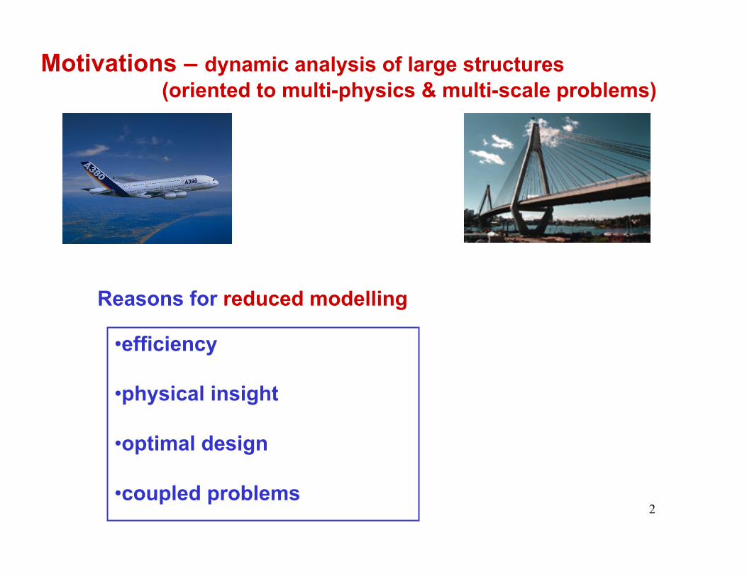
Motivations – dynamic analysis of large structures (oriented to multi-physics & multi-scale problems)
Reasons for reduced modelling
•efficiency
•physical insight
•optimal design
•coupled problems
3
Objectives
Desired features for the reduced model:
•suited for parallel computing
•enables a robust mode selection criterion – adaptativity
•adapted for multi-scale and multi-physics problems
4
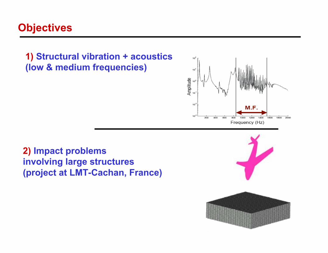
1) Structural vibration + acoustics(low & medium frequencies)
Objectives
2) Impact problemsinvolving large structures(project at LMT-Cachan, France)
5
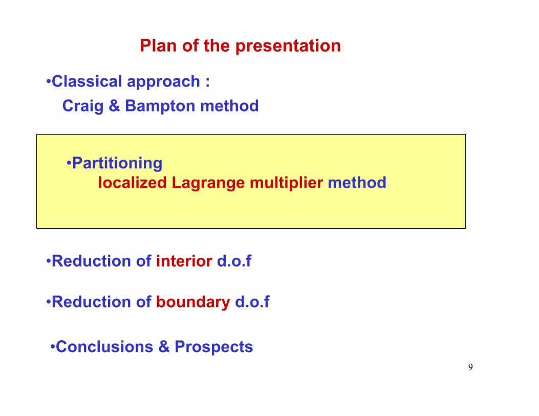
Plan of the presentation
•Classical approach :Craig & Bampton method
•Partitioning
•Reduction of interior d.o.f
•Reduction of boundary d.o.f
•Conclusions & Prospects
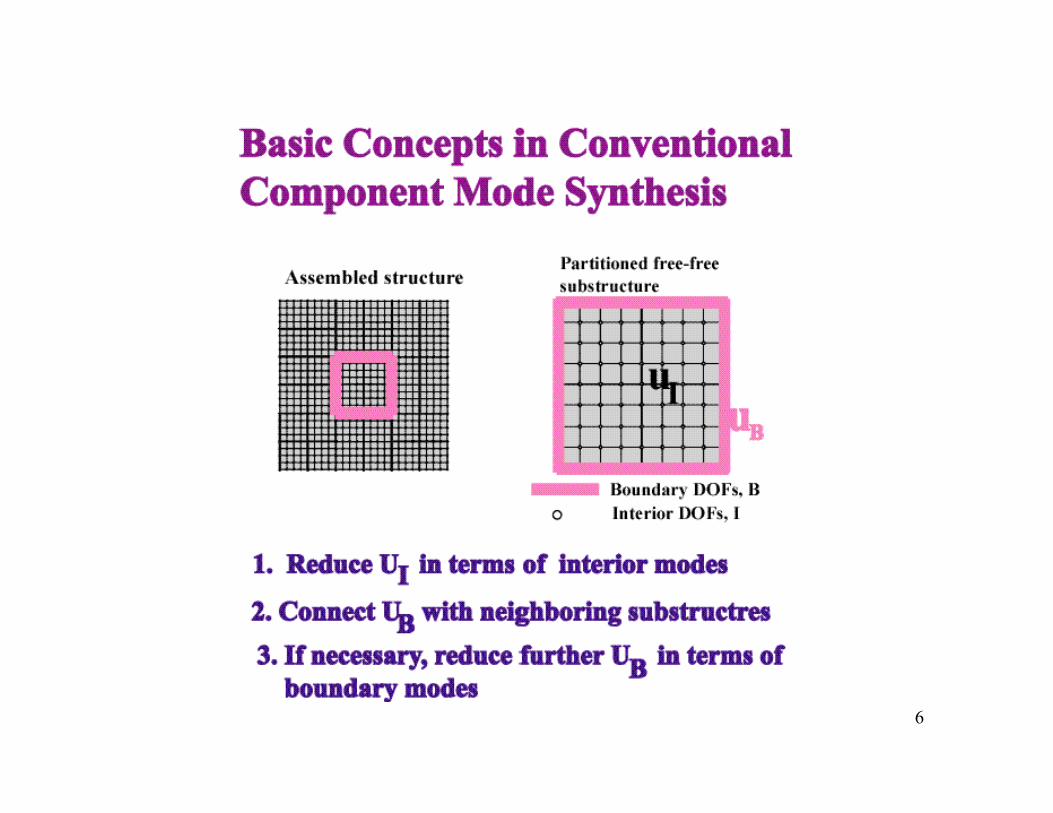
6
7
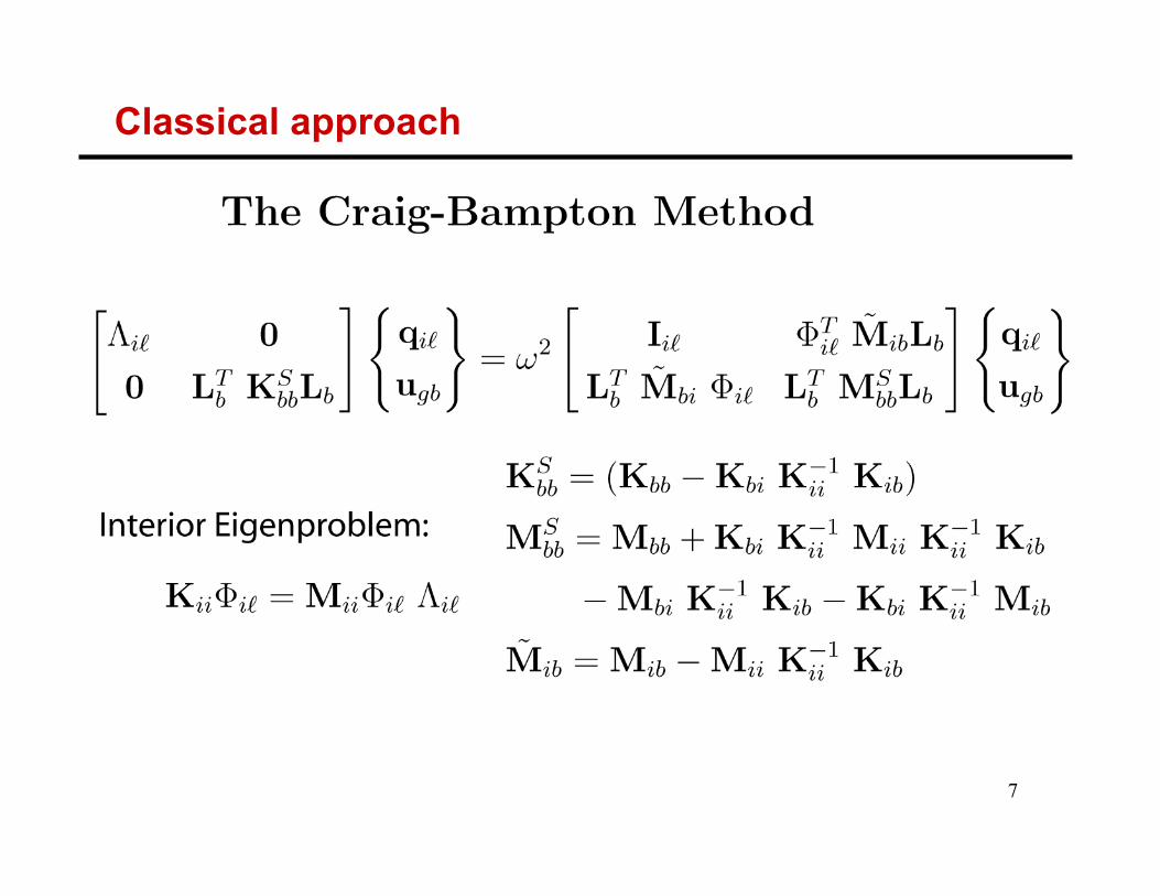
Classical approach
8
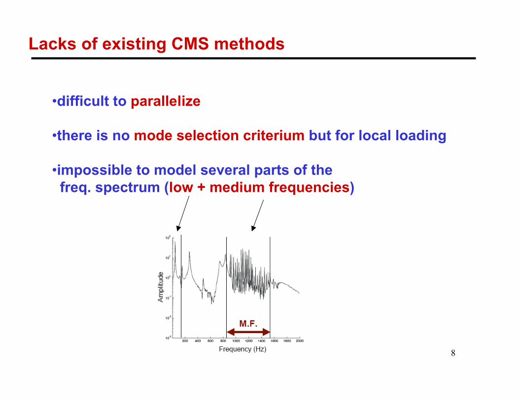
Lacks of existing CMS methods
•difficult to parallelize
•there is no mode selection criterium but for local loading
•impossible to model several parts of the freq. spectrum (low + medium frequencies)
9
•Partitioning localized Lagrange multiplier method
Plan of the presentation
•Classical approach :Craig & Bampton method
•Reduction of interior d.o.f
•Reduction of boundary d.o.f
•Conclusions & Prospects

10
Flexibility based approach - partitioning by localized Lagrange multipliers (LLM)
Park & Felippa et al. 1997-2005
11
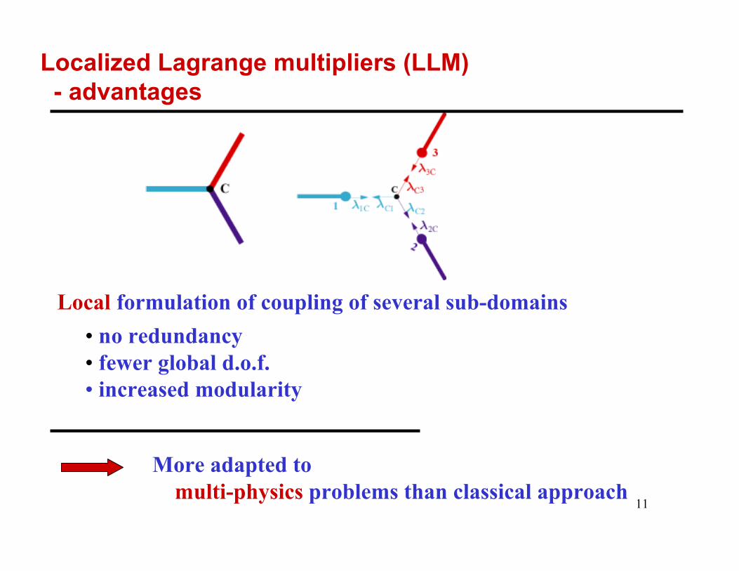
Localized Lagrange multipliers (LLM) - advantages
Local formulation of coupling of several sub-domains• no redundancy• fewer global d.o.f.• increased modularity
More adapted to multi-physics problems than classical approach

12
Localized Lagrange multipliers (LLM) - formulation
Euler-Lagrange equation•Local dynamics
•Global-local compatibility
•Global equilibrium

13
Localized Lagrange multipliers (LLM) - displacement decompositions
zero energy modes (RBM)
deformation modes {,
Reason : substructures being flotting objects
K singular, K-1 non-existent
u = K-1 f, replaced by d = K+ FTf
generilized inverse
But, K+ f ¹u and a = ?
14
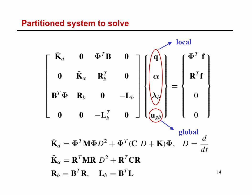
Partitioned system to solve
global
local

15
•Partitioning localized Lagrange multiplier method
Plan of the presentation
•Classical approach :Craig & Bampton method
•Reduction of interior d.o.f
•Reduction of boundary d.o.f
•Conclusions & Prospects

16
Modal decomposition
retained modes residual modes
dim(Fl)† dim(Fr)
17
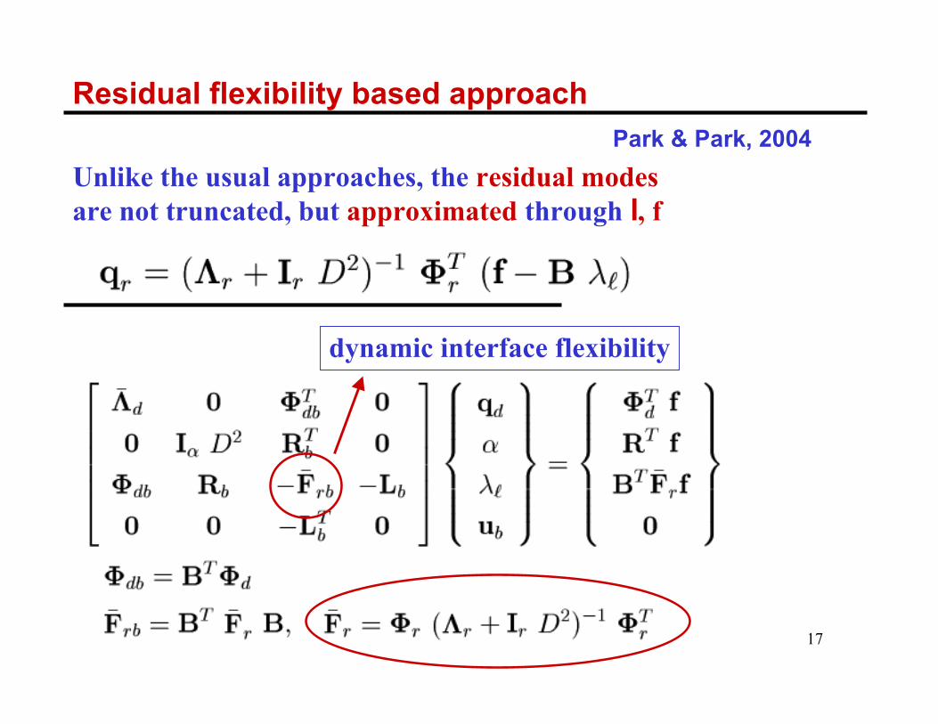
Residual flexibility based approach
Unlike the usual approaches, the residual modesare not truncated, but approximated through l, f
dynamic interface flexibility
Park & Park, 2004

18
Application to the eigenvalue problem
More practical for testing(comparison with exact eigenvalues)

19
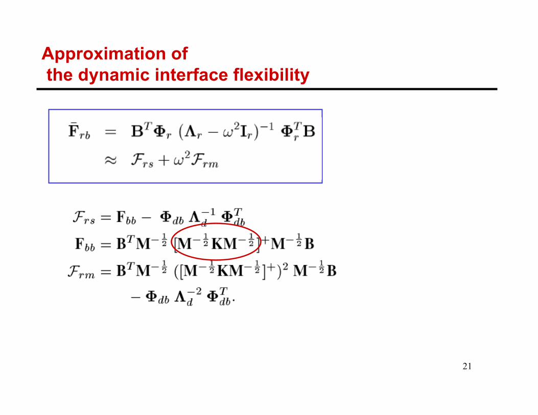
Approximation of the dynamic interface flexibility
Taylor expansion, low frequencies :
20
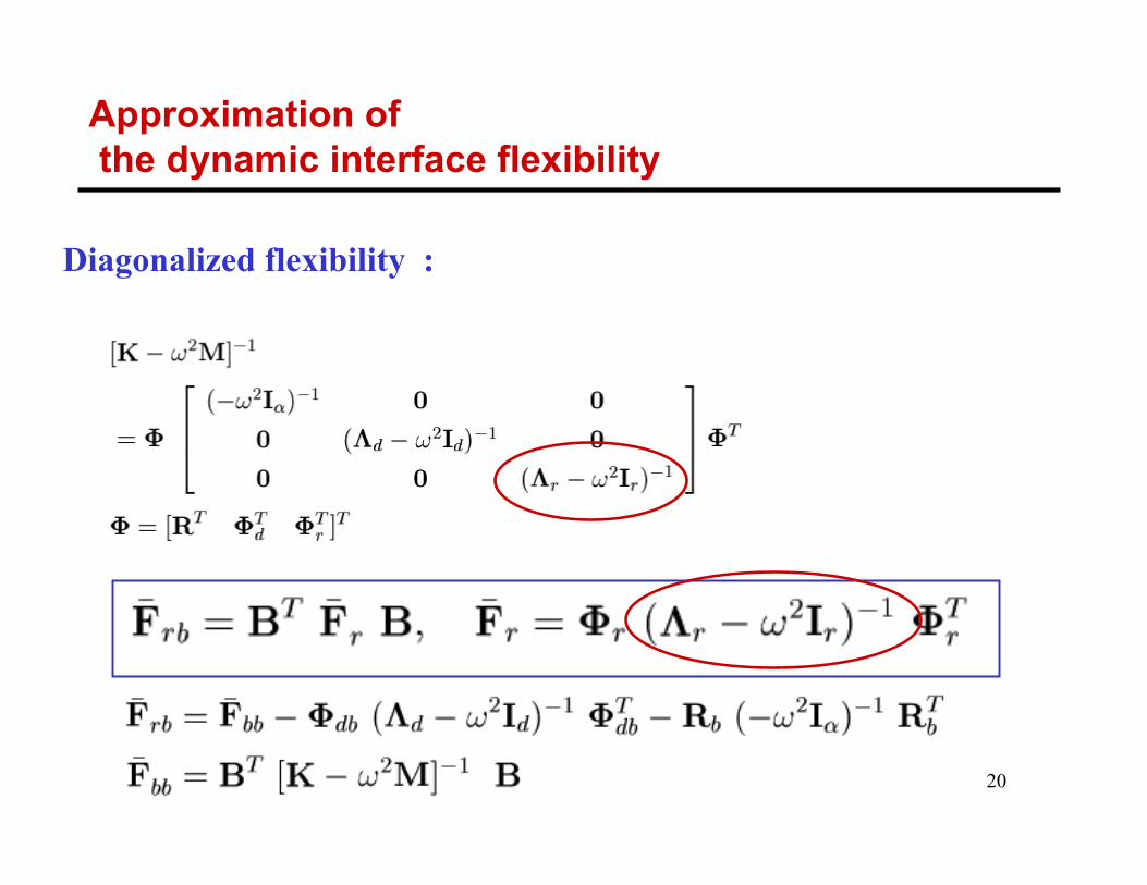
Approximation of the dynamic interface flexibility
Diagonalized flexibility :
21
Approximation of the dynamic interface flexibility

22
Reduced eigenvalue problem
For which exists a very efficient resolution algorithm proposed in Park, Justino & Felippa 1997

23
Mode selection criterion
Idea : find N modes Fd which renders Frb minimal
criterion
Local mode selection ispossible only with LLM

24
Example – thin plate eigenvalue problem
Sub-structure 1 Sub-structure 20.4 0.2
0.3
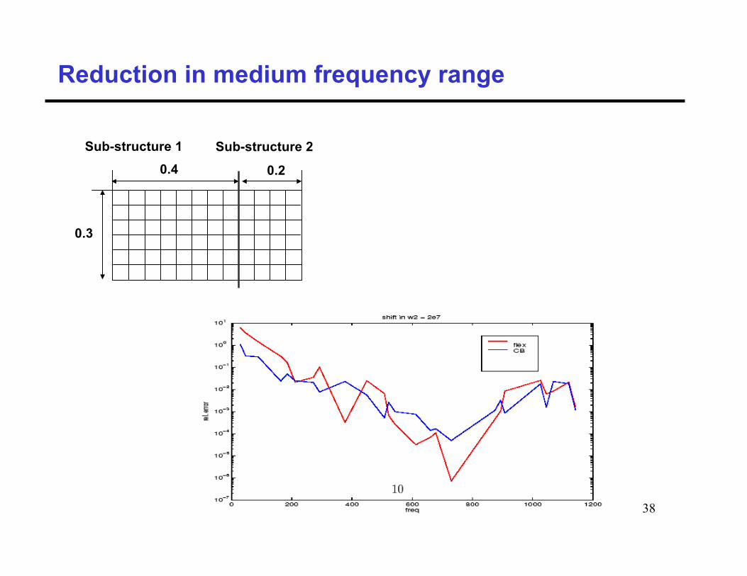
relative error (log)of the eigenfrequency
No of eigen mode
Craig-Bampton method
residual flexibilitymethod
10-4
10-8

25
•Partitioning localized Lagrange multiplier method
Plan of the presentation
•Classical approach :Craig & Bampton method
•Reduction of interior d.o.f
•Reduction of boundary d.o.f
•Conclusions & Prospects
26
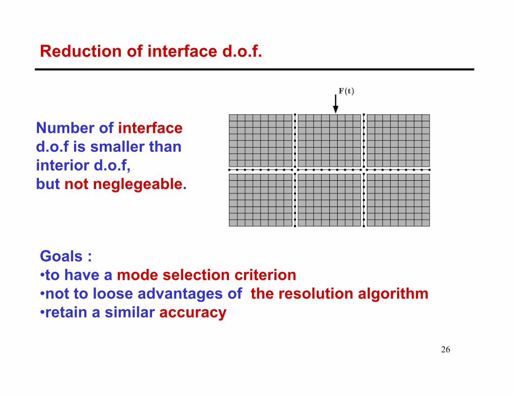
Reduction of interface d.o.f.
Number of interface d.o.f is smaller than interior d.o.f, but not neglegeable.
Goals : •to have a mode selection criterion•not to loose advantages of the resolution algorithm•retain a similar accuracy

27
Reduction of local multipliers - separation from interior modes
ll
l
l

28
Reduction of local multipliers
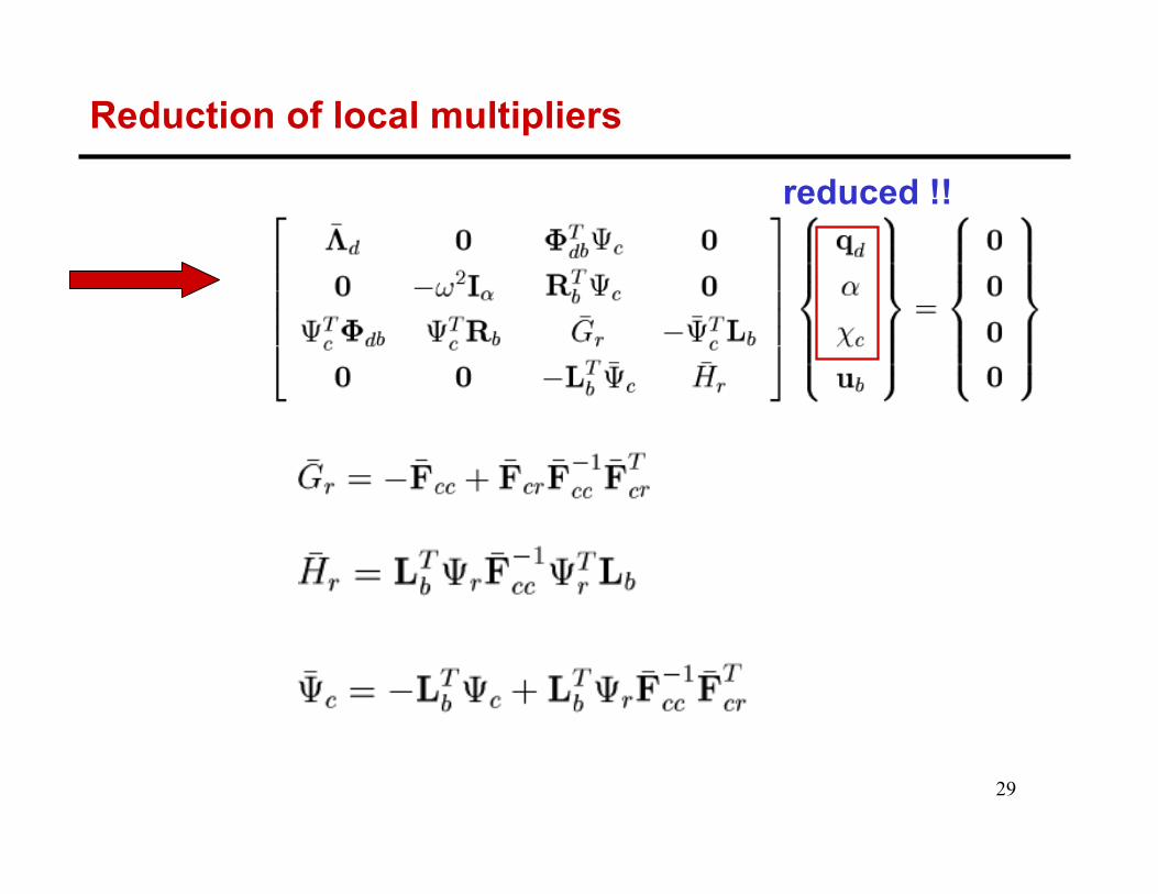
29
Reduction of local multipliers
reduced !!
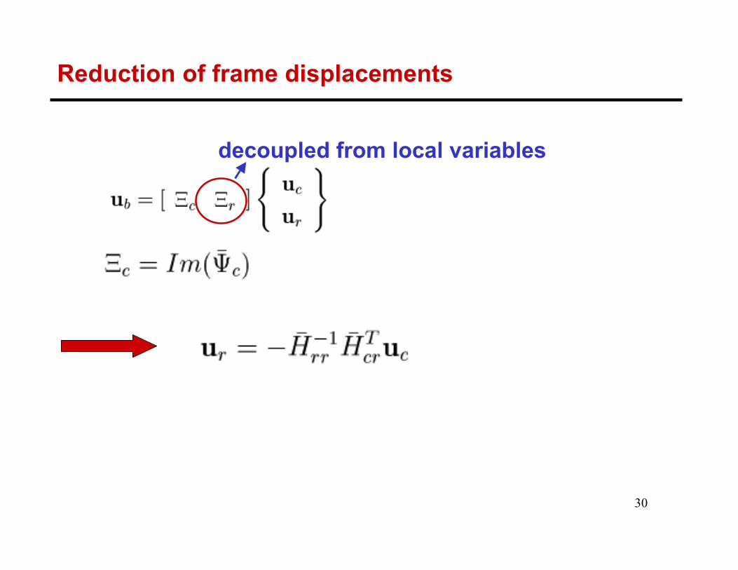
30
Reduction of frame displacements
decoupled from local variables
31
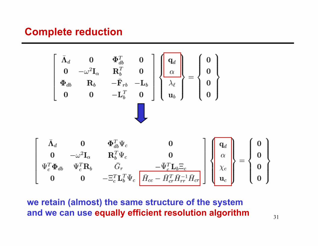
Complete reduction
we retain (almost) the same structure of the systemand we can use equally efficient resolution algorithm

32
Completely reduced eigenvalue problem
partially reduced
fully reduced
No. of modes : Nint + Nint + 3* Nint = 5* Nint
No. of modes : Nint + 2*Nboun + Nboun = Nint + 3* Nboun
exclusively physics dependent
FE model dependent

33
Complete reduction examples – thin plate
2 substructures
Craig-Bampton method
full interface
reduced interface
10-7
10-4
interior 1719 to 19LM 462 to 25frame disp. 231 to 75

34
Complete reduction examples – 3D structure
Z – cross section
Y – cross section
X – cross section
Partitioned
•11 000 d.o.f. FE model
•linear tetrahedra elements
35
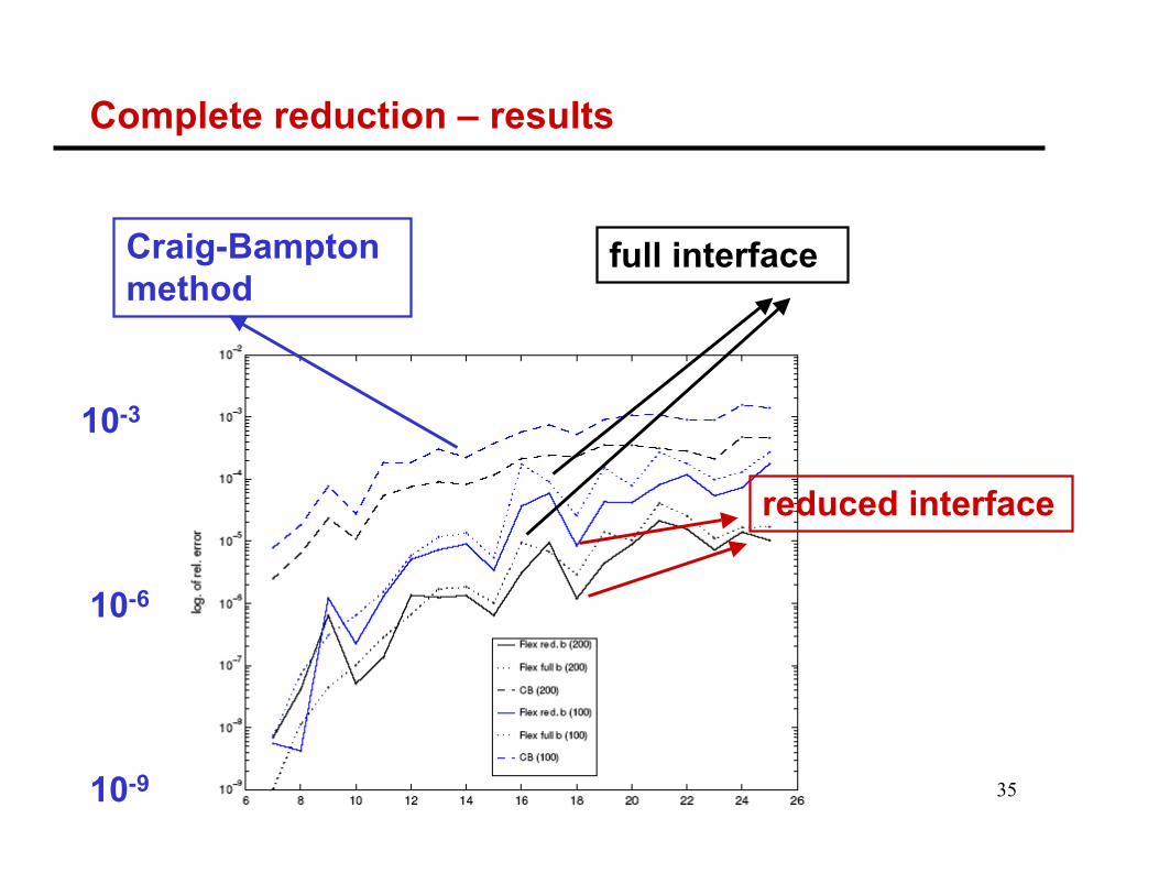
Complete reduction – results
Craig-Bampton method
full interface
reduced interface
10-9
10-6
10-3

36
•Partitioning localized Lagrange multiplier method
Plan of the presentation
•Classical approach :Craig & Bampton method
•Reduction of interior d.o.f
•Reduction of boundary d.o.f
•Conclusions & Prospects
37
Conclusions
•flexibility based approach leads to the consistently reduced models •it is adapted for parallel computing
•mode selection criterion is well established
•suitable for coupled problems
38
Sub-structure 1 Sub-structure 20.4 0.2
0.3
Reduction in medium frequency range
39
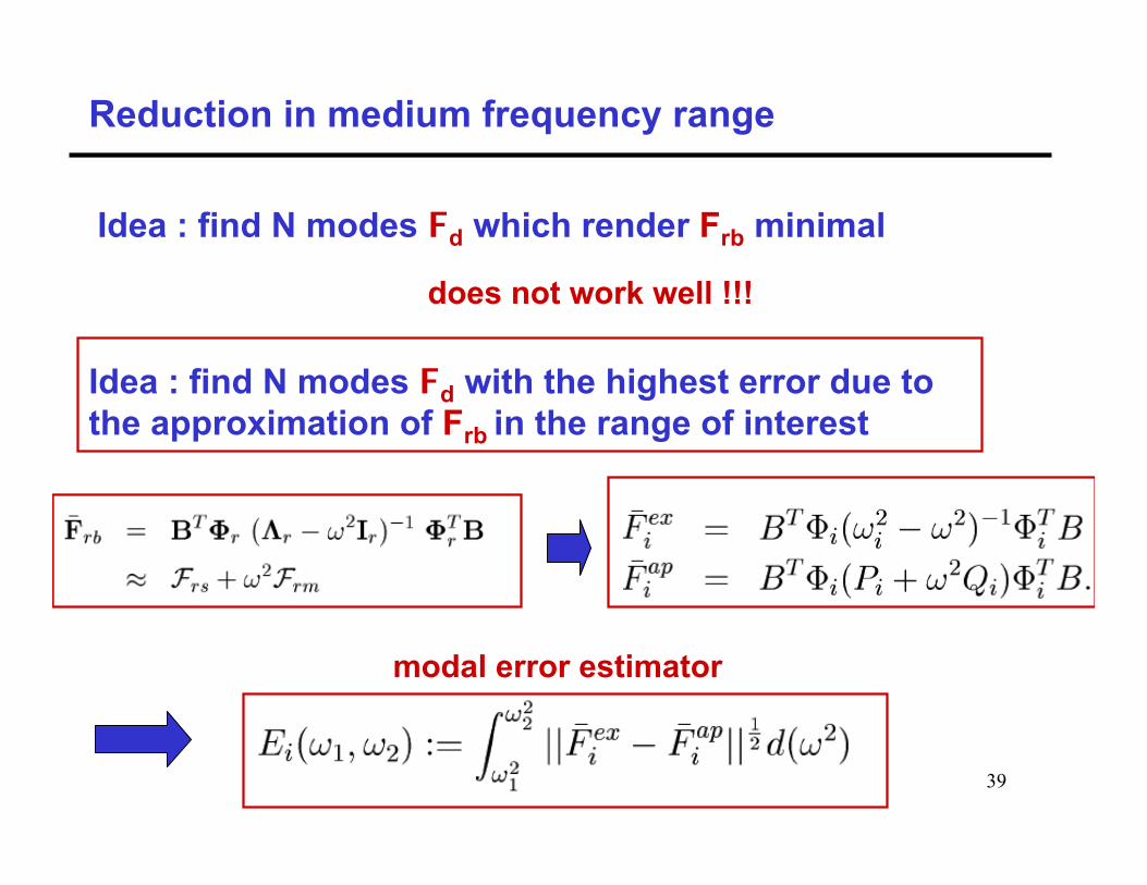
Reduction in medium frequency range
Idea : find N modes Fd which render Frb minimal
does not work well !!!
Idea : find N modes Fd with the highest error due tothe approximation of Frb in the range of interest
modal error estimator

40
Reduction in medium frequency range
low & medium freq. segment
medium freq. segment
Craig-Bampton method
10-6
10-3