path dependence, political competition, and renewable ...mmd2172/papers/computation.pdf · path...
TRANSCRIPT

Path Dependence, Political Competition, and Renewable Energy
Policy: A Dynamic Model
May 6, 2014
Abstract
Climate change mitigation requires sustainable energy transitions, but the political dynamicsof these transitions are poorly understood. This article presents a general dynamic model ofenergy policy with long time horizons, endogenous electoral competition, and techno-politicalpath dependence. Calibrating the model with data on the economics of contemporary renewableenergy technologies, we show that partisan ideology produces large effects on energy policy if thecompeting parties disagree on the importance of energy policy in general. Endogenous electoralcompetition further strengthens these effects, provided the electorate considers energy policyan important issue. In addition, our model displays path dependence in the specific sense thatthe outcome depends on the historical order of elections. The results demonstrate that politicaldynamics could have large effects on the development of renewable energy and carbon dioxideemissions over time.
1
1 Introduction
In the study of environmental political economy, sustainable energy transitions have emerged as a
central topic of interest (Jacobsson and Lauber 2006; Schwoon 2006; Verbong and Geels 2007; Walz
2007; Agnolucci 2008; Loorbach 2010). Defined as “the extensive deployment of clean energy, such
as wind and solar power, to reduce the environmental burden of the national economy” (Aklin and
Urpelainen 2013), such transitions could play an important role in climate change mitigation and
energy security.
To a surprising extent, sustainable energy transitions have already begun in forerunner countries.
While the International Energy Agency predicted in the year 2000 that renewables will continue
to play a negligible role in the energy economy at least until 2020 (IEA 2000), the reality has
proven this pessimistic prognosis wrong. According to the World Development Indicators, in 2012
Denmark generated 48 percent of its electricity from non-hydroelectric renewables. In Germany,
the share was 19 percent. Even in the United Kingdom and the United States, which have begun
investing in renewables much more recently, the shares were 10 and 6 percent, respectively. The
stunning growth rates of renewables and the policies underpinning them highlight the importance
of sustainable energy transitions as a core theme in political science.
Understanding sustainable energy transitions requires paying attention to politics (Torvanger
and Meadowcroft 2011). Fossil fuels continue to dominate the energy landscape largely because
of a market failure, whereby their negative externalities are not priced (Unruh 2000), and gov-
ernment action is needed for a correction (Loorbach 2010). However, government incentives to
promote a sustainable energy transition are still poorly understood. The problem of implementing
a sustainable energy transition is a dynamic one, and governments cannot tie the hands of their
future successors. Despite the growing interest in sustainable energy transitions, there is no fully
dynamic model that would explain and predict the sustainable energy policies of different types
of governments as circumstances change over long periods of time. This is particularly surprising
given that sustainable energy transitions are now widely considered to be slow processes (Ulmanen,
Verbon, and Raven 2009). Such a model would have to allow for long time horizons, endogenous
electoral competition, and techno-political path dependence in energy generation.
2

This article presents the first such dynamic model. In the model, two governments formulate
energy policies over a long time horizon. Our model thus reflects a majoritarian or strongly pres-
idential system. One of the governments is ‘green’ (pro-renewables), while the other is ‘brown’
(anti-renewables). They formulate policy in a dynamic environment with electoral competition and
technological learning. Each government understands that current policies influence both electoral
outcomes and the future competitiveness of clean energy, and the dynamic model allows us to
simulate energy policy trajectories over long periods of time. In practice, we evaluate outcomes for
a period of 50 years. To firmly ground the model in empirical reality, we calibrate the model using
global and U.S. estimates of the parameters characterizing the economics of the energy technologies
considered.
We conduct the analysis against the baseline of a cost-minimizing energy trajectory based on
estimates of the cost and learning curves for renewable energy. In the first political variant of the
model, the two parties have different ideological preferences, but they do not compete for re-election
based on energy policy. The strength of ideology is defined as a deviation from the cost-minimizing
benchmark for renewable energy. For example, the green party is willing to incur some additional
energy costs to protect the environment and mitigate climate change.
This model allows us to isolate cleanly the effects of partisan ideology, without yet considering
the additional effects of competitive electoral strategy. We find that if the two parties are equally
interested in energy policy, their behavior is largely non-strategic. Each party tries to shift energy
policy toward its ideal point, but the optimal strategy is mostly similar to the myopic best response
without political processes. However, if one of the parties is much more ideological about energy
policy, dynamic strategies start to appear. Most importantly, the less ideological party may ap-
pease its more ideological counterpart. In a fully dynamic model with long time horizons, the less
ideological party wants to avoid very high costs from ideological policies by the other party.
The prediction is consistent with macro-political trajectories of industrialized countries. In the
United States, where the conservative movement has, for both political and economic reasons, been
adamantly opposed to renewables (McCright and Dunlap 2003; Laird and Stefes 2009), one could
interpret the slow growth of renewable energy as a result of the left wing’s accommodating tactics.
3
In the United Kingdom, where the conservative position on renewables is less entrenched and more
pragmatic (Toke and Lauber 2007), the left-right gap on environmental and energy policy has
shrunk as renewables have grown (Russel and Benson 2013: 256). Similarly, the societal consensus
on renewables has grown stronger in Germany and Denmark over time (Agnolucci 2007; Laird and
Stefes 2009). This is consistent with the idea that green constituencies with strong preferences
can induce their less enthusiastic, brown counterparts to accommodate, provided the asymmetry
of ideological preference is sufficiently clear.
Next, we endogenize political competition. The partisanship of the government is decided by
a simple “winner take all” election. This modeling approach highlights the ideological contrast
between pro-renewable and anti-renewable parties. It is particularly suitable for national contexts
characterized by a two-party system or stiff ideological competition between conservative and liberal
parties. We find that the qualitative properties of the parties’ strategies remain intact, regardless
of whether the electorate applies a retrospective or forward-looking voting strategy. However, the
electorate is able to partially constrain the parties towards its preferred investment level. The most
important new result is that the pull of the electorate’s preference increases with the ideological
commitment of the two parties. This result is somewhat surprising, as it would be intuitive to
claim that ideological parties do not care about the electorate, as in Laver and Sergenti (2011).
However, more ideological parties hold more diverging preferences over the long-term policy path
and thus they have strong incentives to cater to the electorate to increase their chance of influencing
that policy path. As a result, endogenizing elections has a substantial effect on the mean 50-year
transition paths that we simulate at the end of the paper.
The article builds on and contributes to several strands of scholarship in political science,
economics, and policy studies. Aklin and Urpelainen (2013) present a formal model of exogenous
shocks, path dependence, and partisan ideology in sustainable energy transitions. While their
model accounts for strategic behavior of governments motivated by their constituency interests,
the model is not dynamic and does not account for endogenous electoral competition. They also
do not present a model of technological learning and economies of scale. We add these elements to
our model.
4
List and Sturm (2006) present a model of environmental policy under electoral competition.
They find that under intense electoral competition, politicians implement policies that appeal to
voters with a strong interest in environmental policy. Their model cannot shed light on dynamic
environmental regulation, however, since they assume that a government cannot influence the
behavior of future governments through lock-in effects. We find that forward-looking governments
have incentives to behave quite differently from the myopic governments in List and Sturm (2006).
In economics, dynamic models of environmental policy largely assume benevolent rulers. Fis-
cher and Newell (2008) analyze the relationship between clean technology support and carbon
abatement policies, finding complementarities. Acemoglu et al. (2012) analyze optimal policies for
clean technology in a growth model and characterize the optimal path over time, but they do not
consider the political incentives of governments. Golosov et al. (2011) show that a simple Pigouvian
approach is enough for the optimality of a fossil fuel tax in a general dynamic setting, but the model
does not include any political incentives and problems. Our model shows how the predictions and
policy recommendations for a cost-minimizing planner must be modified when political-economic
considerations are included.
The model presented here has important implications for contemporary energy policy. As multi-
lateral climate negotiations have stalled, scholars are increasingly calling for innovative approaches
to breaking the “global warming gridlock” (Victor 2011). Our dynamic model characterizes the
conditions under which present policy can have significant effects on the future energy trajectories
of societies. Perhaps most importantly, the model provides an analytical foundation for aggres-
sive campaigning and policies by green parties, provided that their brown counterparts are not
as strongly motivated. In the case of the United States, it will be hard for the environmentalists
to break through the policy gridlock, but the outlook for most other countries is much brighter,
as opposition to renewable energy is based on concerns over energy costs, instead of more vested
interests in fossil fuels.
Methodologically, the approach is of interest to computational political scientists. While com-
putational models have been applied to a variety of topics ranging from party competition (Laver
and Sergenti 2011) to international conflict (Cederman and Gleditsch 2004), we are not aware of
5
any political-economy models of environmental or other regulatory policy. Our approach bridges
the traditional divide between analytical approaches based on rational choice and computational
methods that assume simpler behavioral rules. We combine assumptions, premises, and techniques
from both traditions. We show computational power can be used to develop nuanced theories of po-
litical processes without sacrificing the analytical precision that characterizes the modern political
economy literature.
The dynamic modeling approach also contributes to the rapidly growing literature on sustain-
able energy transitions. In this literature, governance and politics are increasingly recognized as
important determinants of energy transitions (Loorbach 2010; Torvanger and Meadowcroft 2011),
but the modeling of such transitions remains a nascent industry. Several longitudinal case studies
offer insights into individual cases (Verbong and Geels 2007; Smith et al. 2014), but a unifying
theoretical framework is missing, making it difficult to unify and consolidate lessons from various
case studies. Our dynamic model is one effort to fill this gap.
The remainder of the article is organized as follows. We begin by presenting a baseline model
of the energy economy with a benevolent social planner. We then introduce partisan ideology,
contrasting the results with the baseline outcome. Finally, we endogenize electoral competition.
Toward the end of the article, we evaluate the implications of these different models for energy
policy and discuss the general significance of the study. A supplementary on-line appendix contains
further details and simulations of the dynamic model.
2 A Baseline Model
In the baseline model, a planner is assumed to follow the cost-minimizing path of energy develop-
ment over a long time horizon. The planner’s interest is simply to generate energy at the lowest
possible total cost, and we do not comment on the normative merits of this approach. The structure
of the model follows Fuss et al. (2008), and is calibrated based on real data for energy technologies.
In selecting the parameters for the model, we rely on global estimates for solar and wind power as
much as possible. For some parameters, such as the cost of solar and wind generation, we use data
from the United States since reliable global estimates are not available. The main drawback of this
6
approach is that it overestimates the potential of renewable energy in some areas and underesti-
mates it in others. Nonetheless, it is a major advance over analytical models that have no basis in
empirical data.
The planner’s strategies are used as a yardstick for investigating the effects of politics on sustain-
able energy transitions. By comparing outcomes under a planner and political decision making, we
can investigate the importance of politics against a conventional benchmark. To maximize realism
and policy relevance, the baseline model builds on canonical models of energy planning.
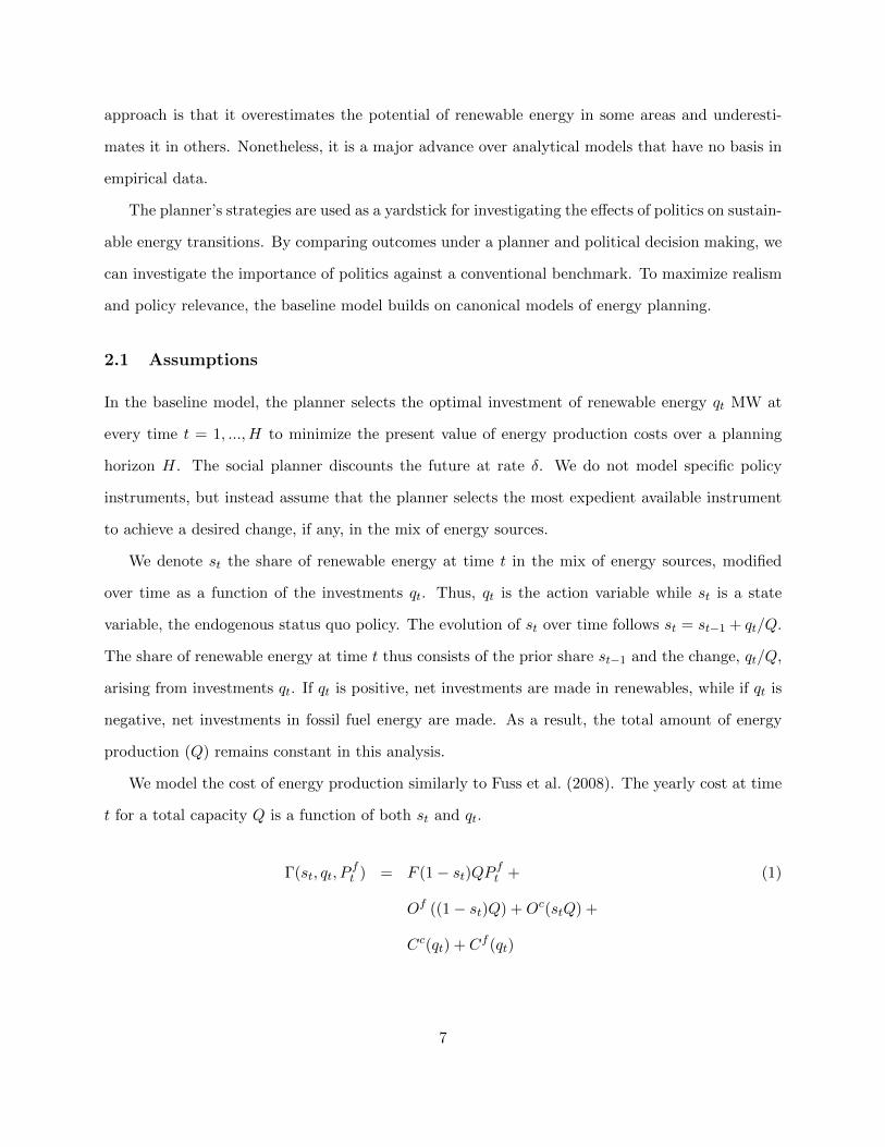
2.1 Assumptions
In the baseline model, the planner selects the optimal investment of renewable energy qt MW at
every time t = 1, ...,H to minimize the present value of energy production costs over a planning
horizon H. The social planner discounts the future at rate δ. We do not model specific policy
instruments, but instead assume that the planner selects the most expedient available instrument
to achieve a desired change, if any, in the mix of energy sources.
We denote st the share of renewable energy at time t in the mix of energy sources, modified
over time as a function of the investments qt. Thus, qt is the action variable while st is a state
variable, the endogenous status quo policy. The evolution of st over time follows st = st−1 + qt/Q.
The share of renewable energy at time t thus consists of the prior share st−1 and the change, qt/Q,
arising from investments qt. If qt is positive, net investments are made in renewables, while if qt is
negative, net investments in fossil fuel energy are made. As a result, the total amount of energy
production (Q) remains constant in this analysis.
We model the cost of energy production similarly to Fuss et al. (2008). The yearly cost at time
t for a total capacity Q is a function of both st and qt.
Γ(st, qt, Pft ) = F (1− st)QP ft + (1)
Of ((1− st)Q) +Oc(stQ) +
Cc(qt) + Cf (qt)
7

This is a standard accounting equation, where the first row represents the cost of fossil fuel. The
second row represents operating costs, and the last row represents capital costs. F is the quantity
of fossil fuel consumed per MW and P ft is the price of fossil fuel inputs, such as coal. Next, Of (·)
and Oc(·) are the operating costs of fossil fuel energy production and renewable energy production,
respectively, as a function of the energy production from those sources, as determined by st. These
assumptions allow both fossil fuels and renewables to have an annual operating cost. Only fossil
fuels have an additional input cost, however, since key forms of renewable energy, such as wind and
solar, are based on free fuel inputs. The terms Cf (qt) and Cc(qt) represent the total capital costs,
respectively, of fossil and renewable energy investment.
We allow endogenous technological learning over time (Nemet 2006; Jamasb 2007; Shum and
Watanabe 2007). We model learning by doing in terms of manufacturing costs. The key advantage
of this approach is that we can use global cost estimates, as the markets for renewable energy
technologies are largely integrated across countries; we will return to the possibility of international
diffusion and spillovers in the concluding section. Specifically, we decompose the capital costs of
renewable energy into two parts. The first part is the per unit capital cost cct , which is subject
to long-term cost reductions due to learning. We use a power law of the total renewable energy
capacity to describe prices under technological learning, which applies to many technologies and
describes trends in capital costs of photovoltaic and wind energy quite well (Nemet 2006).
cct = cc0
(QctQc0
)−α(2)
where Qct = stQ is the installed renewable energy capacity. The coefficient α has a convenient
interpretation if re-expressed as the progress ratio R defined as R = 2−α, which gives the ratio
of the new to old costs under a doubling of cumulative investments. Available data suggests that
αsolar ∈ (0.26, 0.43) and αwind is around 0.15 (Nemet 2006). In what follows, we will use these
values as defaults but let these parameters vary to study the effect of learning on the transition
(see Appendix A1.3). We use current values for price and capacity of solar and wind in the United
States for cc0 and Qc0, as shown in Table 1.
The second component of the renewable energy capital cost function is the total capital costs
8

arising from choosing an investment level qt in a given year, at a per unit cost cct . We assume
that there are strictly increasing marginal costs to adding more units in a given year because of
production capacity constraints. To simplify, the model does not include possible investments to
reduce capacity constraints beyond economies of scale. Hence, the total capital costs for a given
investment level qt > 0 is
Cc(qt, Qct) = ccte
aqt/Qctwhere Qct = stQ (3)
The economy of scale here is independent of technological learning. There is no simple way of
parametrizing the shape of this cost function beyond the long-term learning rates. We have used the
exponential form to preserve units and the parameter a to calibrate equation 3 so that minimizing
equation 2 would result in a 40% renewable energy share in 2050, a goal that is often invoked in
various energy commissions, such as IEA (2012). We have also included a version of equation 2 that
includes a decline in the rate of learning, drawing on assessments of future investment paths made
available in Lantz, Hand, and Wiser (2012), so as not to extrapolate the past learning experience
beyond plausible ranges (see Appendix, A1.1.1). The construction costs of fossil fuel plants (Cf (·))
are linear in new capacity, where qt < 0. Notation for the baseline model and the values used for
fixed parameters are summarized in Table 1.
[Table 1 about here.]
2.2 Characterizing the Economic Optimum
We solve the dynamic model using dynamic programming in a structure similar to Fuss et al.
(2008). The algorithm determines the optimal action for each state of the world and each time
step over the planning horizon. The state of the world at any point in time is described by the
share of energy produced by clean technologies (st) and the price of fossil fuel (P ft ). The possible
actions in each state are discrete levels of investment in or disinvestment from clean energy (qt).
The economically optimal investment from each state is denoted qEt (st−1, Pft ). It represents the
choice that minimizes the discounted sum of all energy expenditures (fuel costs, operating costs,
9

and construction costs), as described above. Throughout, we will refer to this in terms of the
optimal share, denoted sEt = st−1 +qEt (st−1,P
ft )
Q . This is an implicit function of the current state,
not an exogenous trajectory.
Fuel prices evolve stochastically according to an AR(1) process to which, in some experiments,
we add an increasing time trend (Appendix, A1.1.2). One of the strengths of a computational
approach is that we can solve for rational policies despite uncertainty about fuel prices in the
future. We estimate the evolution of prices using Monte Carlo simulations at each step in the
planning horizon. We can express the decision problem as a Bellman equation,
Vt(s, Pf ) = min
qΓ(s, q, P f ) +
e−δ
n
∑i
Vt+1
(s+
q
Q,MCi(P
f )
)(4)
The value function is described in terms of the share of renewable energy, s, and the price of
fuel, P f . We average over all Monte Carlo simulations of the fuel price evolution, MCi(Pf ) for
i = 1 . . . n, to determine the discounted value as a function of future fuel costs.
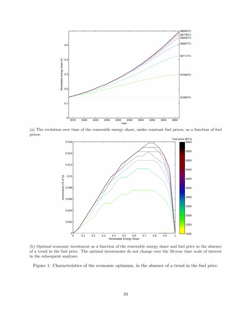
The model is solved using backward induction in Matlab. The outcome under a planner is
illustrated in Figure 1. The upper panel shows the path of the share of renewable energy in the
absence of a trend in the fuel price, which is the result of applying the optimal strategy shown in
the lower panel. Each path is characterized by a constant fuel price, but the optimization yielding
the strategies is based on the assumption of stochastic fuel prices with no trend in the fuel price. At
a fuel price of $1000/TJ, additional clean energy construction is not optimal under the 5% discount
rate used here. As the fuel price increases, so do the optimal investments. Above $4000/TJ, optimal
investment curves are very similar. This is due to the convexity of the cost function for new clean
energy capital. When investments in renewable energy are large, the convexity of the cost function
ensures that additional fuel price increases have little effect on the optimal investment level.
[Figure 1 about here.]
In the lower panel, we see that optimal investments are maximal at intermediary levels of the
existing renewable energy share, which explains the initial exponential shape of the paths in the
upper panel. When the renewable energy share is low, investments are hampered by the higher
10

capital costs stemming from the absence of prior technological learning. When existing shares are
very high (> 70%), investments are also low because little additional benefit can be gained.
The results are sensitive to both the price process and the rate of technological learning. In-
creasing the volatility of the AR(1) price process quite naturally diminishes the importance of the
current price in determining the level of optimal investments. Thus, a high price volatility warrants
substantial increases in investments even at the lowest energy price (such that for a doubling of our
baseline volatility parameter, investments worth 0.5% of Q per year are called for when the price
is at its lowest). Conversely, if there is very little volatility, optimal investments increase at high
energy prices (Appendix, A3). Adding a moderate trend to the price causes investments at lower
present prices to increase (Appendix, A4, and A2).
Finally, the learning parameters have an important effect on investment strategies and the path
of investments. For all states of the world, a higher learning rate causes optimal investments to
increase, especially at intermediate stages of the transition (Appendix, A5).
3 Political Polarization
In the next iteration of the model, we add political polarization by introducing a ‘brown’ and
‘green’ party (denoted B and G respectively) with differing energy preferences (Shipan and Lowry
2001; Neumayer 2003). The brown party is opposed to renewable energy, while the green party is
supportive of renewables. For example, members of the green party could be worried about the
global environmental effects of fossil fuels. In this variant of the model, electoral outcomes do not
depend on energy policy. Therefore, the variant can be used to identify the effects of political
polarization on sustainable energy transitions without electoral considerations (Urpelainen 2012).
However, both parties account for the possibility of losing elections (Alesina and Tabellini 1990).
3.1 Model Description
The two ideological parties hold intrinsic preferences over energy policy outcomes over all periods,
independently of whether or not they are in power. This assumption is based on the idea that
politicians are, at least to some extent, motivated by policy (Moe 2005; Hovi, Sprinz, and Underdal
11
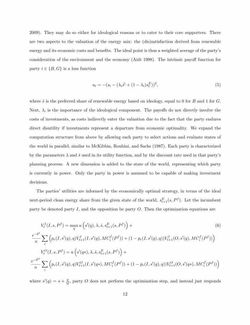
2009). They may do so either for ideological reasons or to cater to their core supporters. There
are two aspects to the valuation of the energy mix: the (dis)satisfaction derived from renewable
energy and its economic costs and benefits. The ideal point is thus a weighted average of the party’s
consideration of the environment and the economy (Aidt 1998). The intrinsic payoff function for
party i ∈ {B,G} is a loss function
ut = −(st − (λisi + (1− λi)sEt ))2, (5)
where s is the preferred share of renewable energy based on ideology, equal to 0 for B and 1 for G.
Next, λi is the importance of the ideological component. The payoffs do not directly involve the
costs of investments, as costs indirectly enter the valuation due to the fact that the party endures
direct disutility if investments represent a departure from economic optimality. We expand the
computation structure from above by allowing each party to select actions and evaluate states of
the world in parallel, similar to McKibbin, Roubini, and Sachs (1987). Each party is characterized
by the parameters λ and s used in its utility function, and by the discount rate used in that party’s
planning process. A new dimension is added to the state of the world, representing which party
is currently in power. Only the party in power is assumed to be capable of making investment
decisions.
The parties’ utilities are informed by the economically optimal strategy, in terms of the ideal
next-period clean energy share from the given state of the world, sEt+1(s, Pf ). Let the incumbent
party be denoted party I, and the opposition be party O. Then the optimization equations are
V It (I, s, P f ) = max
qu(s′(q), λ, s, sEt+1(s, P
f ))
+ (6)
e−δI
n
∑i
(pe(I, s
′(q), q)V It+1(I, s
′(q),MCfi (P f )) + (1− pe(I, s′(q), q))V It+1(O, s
′(q),MCfi (P f )))
V Ot (I, s, P f ) = u
(s′(q∗), λ, s, sEt+1(s, P
f ))
+
e−δO
n
∑i
(pe(I, s
′(q), q)V Ot+1(I, s
′(q∗),MCfi (P f )) + (1− pe(I, s′(q), q))V Ot+1(O, s
′(q∗),MCfi (P f )))
where s′(q) = s + qQ , party O does not perform the optimization step, and instead just responds
12

to the action chosen by party I, which is denoted as q∗. The stochastic Monte Carlo simulations
results are now divided into MCf , the fuel price evolution, and pe, the probability of the incumbent
party being elected. pe is 1 on non-election years. Note that the first parameter of both V I and
V O is I, since these equations reflect the decision-making process when party I is in power. We
solve the corresponding equations separately for states of the world where party O is in power.
3.2 Results
Results from a computational model are not analytical propositions, but rather results that are
robust to variation in parameter values and across simulations. We summarize here the key insights
on the role of political polarization.
To begin with, we characterize the effect of ideological divergence on investment. By ideological
divergence, we refer to increases in λB and λG. An increase in λi makes party i more willing to
sacrifice economic welfare for achieving an ideological preference in energy policy.
Result 1. As λB and λG increase, investment in renewable energy investment strategies increas-
ingly depart from the economically optimal investment path.
This result shows that ideological divergence produces the same results as in the analytical
model of Aklin and Urpelainen (2013). As partisan polarization increases, brown and green parties
choose increasingly diverging strategies. Each deviates from the economically optimal strategy.
The result is illustrated in Figure 2. Even for modest values of λ, the brown party always invests
in fossil fuels. For almost all values of λ, strategies of the parties are monotonically decreasing in
the share of clean energy. The strategies are in the positive investment range for the green party
and in the negative investment for the brown party.
[Figure 2 about here.]
Although obtained by dynamic optimization, the investment strategies are virtually identical
to the choices of hypothetical actors who only considered their present-period payoffs without
any dynamic strategizing. The reason is that any attempt to modify the path of future play by
the incumbent would be later offset by actions of the opposition party. Each party understands
13

that if it increases or decreases the level of investment in renewable energy, the competing party
responds with the diametrically opposed strategy. Deviations from the economic optimum are
expensive and, given the reaction of the competitor, not optimal. Despite partisan polarization
dynamic strategies over energy policy turns out to play a relatively modest role, contradicting
arguments (Hovi, Sprinz, and Underdal 2009) and analytical results (Aklin and Urpelainen 2013)
from the previous literature. Although the energy transitions literature tends to emphasize long
time horizons (Verbong and Geels 2007; Loorbach 2010; Urpelainen 2012), we find that if both
parties are equally ideological, their political strategies actually resemble the maximand of the
party’s utility function (equation 5). This corresponds to the investment the party would choose if
there was no future interaction with the other party and hereafter we will call it the myopic policy.
The following result sheds further light on when strategic incentives play a role in this system.
We now relax the assumption that both parties are equally ideological, allowing differences in their
ideological commitments.
Result 2. Let ∆λ = |λB − λG| denote the difference in the ideological strength of the parties.
As ∆λ increases, departures from the presently preferred strategies of parties increase due to the
dynamic strategic effects arising from technological lock-in.
If the two parties are ideological to differing degrees, then behavior becomes strategic. For
example, it could be that the brown party just wants to implement the economic optimum, while
the green party is worried about the global negative effects of fossil fuels, such as climate change.
In this case, the green party’s ideological commitment |λG| is stronger than the brown party’s
commitment |λB|. Consequently, partisan strategies become increasingly complex.
Figure 3 shows the investment strategies of the parties as λG increases, while λB is kept constant.
That is, the green party becomes increasingly ideological, while the brown parties remains at a
relatively low level of ideology. Although λB stays constant, its optimal strategy changes as a
function of λG. In particular, when λG is high and the green party’s strategy departs significantly
from the economic optimum, the brown party increases investment in s in order to bring the
economy into a state where the actions of the green party are more economically optimal. At a
higher s, the actions of the green party are closer to economic optimality, and this reduces the cost
14
of clean energy investment. Strikingly, the brown party invests more in renewable energy to prevent
the green party from imposing extremely high costs on the economy through the rapid scaling of
renewable energy. This strategy may initially appear counterintuitive, but it is entirely rational.
By accommodating the highly ideological green party, the brown party avoids the high economic
costs of a crash program of renewable energy deployment coveted by the environmentalists. If the
brown party chose a lower level of investment, the green party would go all out and make expensive
investments to promote renewable energy.
From a bargaining perspective, the green party’s threat of paying a high cost for renewable en-
ergy is sufficiently credible to induce the brown party to compromise (Schelling 1960). Interestingly,
this pattern of behavior is the exact opposite from Aklin and Urpelainen (2013). In their model,
political polarization always results in more extreme strategies because the model does not allow
asymmetric ideological commitments. Our computational model shows that this kind of asymme-
try in the strength of an ideological commitment may reverse the sign of the expected effect, with
notable substantive implications.
[Figure 3 about here.]
Figures 4 and 5 show that the effect of the re-election probability p on investment choices is
also conditional on the difference in ideological strength of the parties. Variation in strategy due
to p indicates that parties find it worthwhile to manipulate the future path of play and diverge
from the actions they would prefer if they only considered their present-period payoff since p only
affects the continuation value of the game.
[Figure 4 about here.]
[Figure 5 about here.]
The difference between Figures 4 and 5 reinforce that for dynamic strategic incentives to have
an effect in this system, it is necessary that ∆λ 6= 0. When ∆λ = 0, both parties care about their
ideologically preferred policy to the same degree and discount the future to the same degree. As a
result, any deviation today from one’s preferred course of action done to impel the other to change
15

its investment strategy is offset by the other parties equal commitment to move policy in the other
direction. In this scenario, for all re-election probabilities, the parties have the same investment
strategies, which follows the same trend as the economically optimal one (relative to sT and P f ),
albeit shifted up or down by the extent of their ideological preference.
Asymmetry in the election probabilities has little effect when parties are equally ideological,
but it becomes important when there is also an ideological asymmetry between the parties. In the
asymmetric scenario under consideration (∆λ 6= 0), the green party is more ideological than the
brown party. When the brown party’s chance of being elected are very low, party G follows the
same investment strategy as in the symmetric scenario. However, as the brown party’s chance of
election increases, so do the green party’s investments: G seeks to influence B who puts most weight
on economic optimality. The brown party, although not very ideological, is nonetheless pulled by its
own strategic motives: because the green party tends to over-invest relative to economic optimality
especially when the clean energy share is low, the brown party in fact raises its investments when
it has a low probability of being in power, to shift the status quo to a level where the green party
will be closer to the economically optimal course.
The variation over time in the strategies under the above scenarios are shown in the Appendix
(A2). When ∆λ = 0, the strategies hardly vary over time. However, when they differ, there are
clear election-year cycles driven by the strategic lock-in effect. There also are some longer time
trends, whereby the parties relax towards their presently preferred strategies towards the end of
the planning horizon.
To summarize, the key finding from this model variant is that divergence in the strength of
the ideological commitments of the two parties is essential to understanding their strategy. If both
parties are equally ideological, their incentives are mostly similar to those in a myopic optimization
model. But as the strength of ideological commitments starts to diverge, dynamic strategies become
more common. Most importantly, the less ideological party starts to accommodate the other to
avoid expensive crash investments. As stated in the introduction, this is consistent with the ability
of green parties to forge – to a certain extent – a societal consensus on renewables in Denmark,
Germany, and, more recently, the United Kingdom. In the United States, where the ideological
16

opposition to renewables and economic dependence on fossil fuels is much higher, this has not been
the case. According to our model, a change in ideology would be required to qualitively change
this state of affairs.
4 Endogenous Political Competition
The final version of the model introduces endogenous political competition. Given the importance
of dynamics for energy policy, standard analytical approaches are not suitable for modeling the con-
sequences of political competition for renewable energy deployment over time. The voters consider
the energy policy of the incumbent government in deciding whether to support the incumbent or a
political competitor. By comparing this third version of the model with the political polarization
variant, we can uncover the role of the electorate in shaping the dynamic incentives of political
parties to invest in renewable energy. As we will see, the more ideological the parties, the greater
their stake in strategically controlling the transition path, and the greater their incentive to satisfy
the electorate in order to stay in office and continue to control energy policy. For this reason, even
a weakly responsive electorate has an influence on the transition strategies deployed by the parties.
4.1 Model Description
The electorate compares either the recent performance or the policy platforms of the two parties.
That is, we consider both “retrospective voting” (Fiorina 1981; Ferejohn 1986) and forward-looking
voting based on policy platforms (Downs 1957; Enelow and Hinich 1984). Since both approaches to
voting are plausible, it is important to investigate if the results depend on the behavior of the voting
population. In both variants, the re-election probability of the incumbent increases or decreases as
a function of how much more favorable it seems to the electorate relative to the opposition. The
electorate is sensitive both to the ecological impact of the energy mix and its economic optimality.
To keep the analysis tractable, we model the electorate in an aggregated way, stipulating a
median preference for the electorate. Formally,
se∗t = λe + (1− λe)sEt (7)
17

is the preferred renewable energy share of the electorate at time t, where the electorate puts weight
λe ∈ [0, 1] on having an economy based 100% on renewable energy and weight 1− λe on economic
optimality. These preferences over states of the world induce preferences qe∗t over investment
actions qt, which are represented in Figure 6 for different values of λe and contrasted to those
of the parties. This formulation allows us to examine the relationship between the population’s
environmental preferences and energy policy.
Let qit represent the investment by party i ∈ {A,B} at election period t. Then, let ∆ =
|qe∗t − qBt | − |qe∗t − qAt | measure the relative improvement for the electorate in party A’s over party
B’s policy. Let p be the probability of election of party A, a function of ∆. If ∆ = 0, then both
parties are equally far apart from the electorate’s preferred policy, and thus p = 0.5. In what
follows, we let p vary as a function of ∆ as in Figure 6 and described by the following equation:
p =
0.5 + b log(a∆ + 1) if ∆ ≥ 0
0.5∆− (b log(−a∆ + 1)− (0.5(1−∆))) if ∆ < 0
(8)
In this formulation, b determines how much the probability of an electoral victory depends on
energy policy. As b increases, energy policy becomes more important as an issue in the elections.
In our analyses, we use b = 0.5, reflecting reasonably weak electoral sensitivity to energy policy.
Additionally, we set a = e0.5/b− 1, which ensures that p = 1 when ∆ = 1 and p = 0 when ∆ = −1.
[Figure 6 about here.]
We first implement a retrospective voting variant of this model. In this model, the electorate
compares qIt−1, the policy implemented in the previous period by the incumbent party to qOt−1, the
policy the electorate assumes would have been adopted by the opposition period if in power. In
this case, ∆ = |qe∗t − qOt | − |qe∗t − qIt | and p(∆) according to equation 8 represents the re-election
probability of the incumbent. Reasonable choices for qOt are the economically efficient investment
qEt , or the myopic policy, qO∗t , the maximand of the party’s utility function. Since the policy choices
of the parties are sequential, we can use the same dynamic optimization algorithm as above. The
optimization equations are identical to equation 6, except that the Monte Carlo election function
18

depends on qt, qEt (·), and the state of the world. For further details, see the Appendix A3.1.
4.2 Results
We start this section by showing that the qualitative results from the model without endogenous
electoral competition remain unchanged if we introduce elections.
Result 3. Results 1 and 2 of the exogenous election variant of our model are maintained under
endogenous elections. First, as ideological strength increases, partisan strategies are pulled away
from economic optimality. Second, when ideological commitment is asymmetric between the parties,
dynamic strategic incentives arise due to technological lock-in.
This result shows that the qualitative results under exogenous election are robust to making
elections endogenous. The figure illustrating this, to be compared to Figure 2, is available in
Appendix A3.2. Even with endogenous elections, the strategic logic described above remains intact.
This result, however, does not mean that elections have no effect on strategies. As we will see below,
elections have quantitatively strong effects on policy. However, because parties care not only about
election but also about policy outcome, they trade off their policy preferences and their electoral
advantage. As a result, the parameters driving their preferences still have the same qualitative
effect on strategies. In particular, it is still the case that parties seek to manipulate the status quo
in order to influence the future path of play when ∆λ 6= 0.
The following results highlight how endogenous elections change the outcomes of the interaction.
Let αi = qi∗t − qit, where i = G or B, denote the difference between party i’s preferred investment
without politics (qi∗t ) and its chosen investment given dynamic electoral incentives (qit).
Result 4. When the ideological commitment λi of the two parties is equal, αi has a sign (–/+)
such that each party’s strategy is closer to that preferred by the electorate, irrespective of the current
state of the world, with endogenous electoral competition as compared to the case without.
This latter result is as we would expect. Endogenous elections make the policies responsive
to the public’s preferences. Specifically, the brown party’s strategy now systematically involves
more investment in renewables than without the electoral response. The green party’s strategy
19

involves more or less investment in renewables depending on the weight put by the electorate on
the environmental dimension.
Figure 7 illustrates this. Here we see that for some values of λe, the investments of both
parties come closer to each other, towards the electorate’s moderate environmental concerns. For
larger values of λe, both parties’ strategies are shifted by a similar amount upward, to partially
satisfy a greener electorate. Thus, unlike in the exogenous elections case, parties depart from their
instantaneously preferred strategies. They do so to improve their probability of election, but as the
lower panels of Figure 7 show, the parties are willing to compromise their chances of re-election.
In those panels we see that the changes in the probabilities of re-election varies with λe as well as
with the state of the world. The result that follows provides comparative statics with regard to the
magnitude of the departures αi.
[Figure 7 about here.]
Next, we consider the relationship between ideological strength and the electoral pull.
Result 5. When the ideological commitment λi of the two parties is equal, αi increases with λi.
This result is less intuitive. The more ideological the parties are, the more responsive they are to
the electorate, in the specific sense that their chosen actions increasingly depart from their preferred
actions in absolute terms. This does not mean that both parties end up closer to the electorate.
Indeed, they do not. Figure 8 illustrates these relationships. The political line shows the distance
between the electorate’s wishes and the action actually chosen by party i (this can be denoted
αie,pol = qe∗t − qit), while the apolitical line shows the distance between the preferred action of the
electorate and the apolitically preferred action of party i (this can be denoted αie,apol = qe∗t − qi∗t ).
Here, αi is the wedge between the two lines since αi = αie,apol − αie,pol. As λi increases, we see that
this wedge increases, as stated in Result 5. The distance of the brown party from the electorate
(αBe,pol) nonetheless increases with ideological strength.
[Figure 8 about here.]
The distance of the green party from the electorate also increases when the electorate wants eco-
nomically optimal strategies, while it decreases with λi if the electorate is strongly pro-renewables.
20
This change in direction is understandable in light of Result 4. The important feature is that the
slopes of the solid lines – how the distance between parties’ actions and the electorate’s wishes
changes with ideological strength – are not as steep as the slopes of the dashed lines (change of
αie,apol, the distances of the parties from the electorate in the absence of political competition).
Hence, the constraining effect of elections grows with the strength of ideology
Results 4 and 5 hold exactly when ∆λi = 0, that is, when ideological commitments are equally
strong. When ∆λi 6= 0, electoral incentives interact with the dynamic incentives of technological
lock-in. If λG > λB, the two effects go in the same direction since the electorate is pro-renewables,
and both parties are seeking to raise investments due to technological lock-in (as was illustrated in
Figure 3). In the interesting scenario when λB > λG, the two effects compete, pulling in different
directions. The parties want to reduce their investments because there is more policy agreement
between the parties when s is low. Depending on the strength of the electoral incentives b, αi has a
sign that increases the distance between party i and the electorate, for both parties (see Appendix
for an illustration).
4.3 Robustness to Assumptions about Voting Behavior
Our second variant of the endogenous election model assumes a forward-looking electorate that is
evaluating the competing platforms of the two parties. We thus compute ∆ and p(∆) on the basis
of the policy platforms of both parties at the time of election. This variant induces a normal-form
game in each election period, where each party must choose its platform based on its expectation
of the other party’s platform. Choices are no longer purely sequential. To solve the election period
stage games induced by platform competition, we use the cognitive hierarchy model developed by
Camerer, Ho, and Chong (2004), a bounded rationality algorithm for solving normal form games
that identifies a unique equilibrium and has been shown to predict people’s actions better than the
Nash model over dozens of different experimental data sets and normal game forms. The approach
is similar to the approach used in Laver and Sergenti (2011). The cognitive hierarchy algorithm
is described in greater length in the Appendix A3.3. The results of the platform competition are
barely distinguishable from those of our retrospective implementation. A party’s best response to
21
the electorate’s assumption about the opposition is similar to a party’s best response to his own
assumption about what the opposition is about to do, if these assumptions are similar.
5 Sustainable Energy Transitions: Comparative Statics and Sce-
narios
The previous two sections have presented the properties of energy policies as a function of different
states of the world and under different assumptions about decision-making.. We can now see how
these policies unfold and produce outcomes in the long run. We first illustrate the paths generated
by different scenarios and then present more systematic comparative static results.
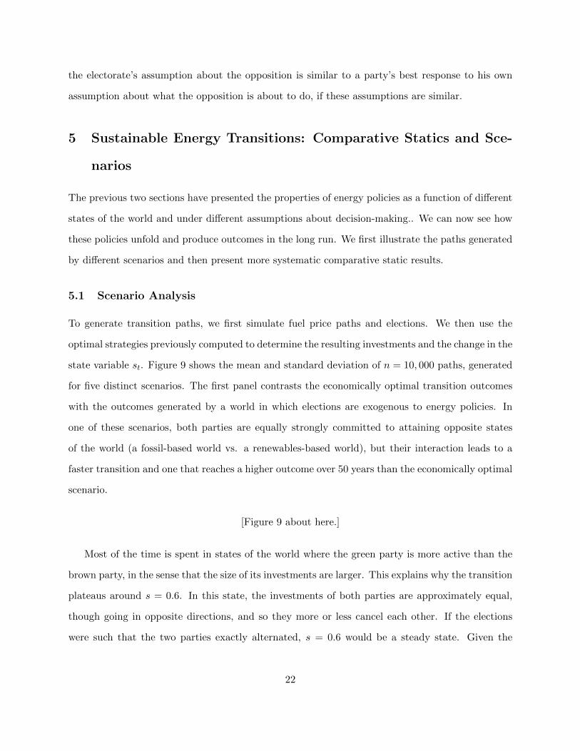
5.1 Scenario Analysis
To generate transition paths, we first simulate fuel price paths and elections. We then use the
optimal strategies previously computed to determine the resulting investments and the change in the
state variable st. Figure 9 shows the mean and standard deviation of n = 10, 000 paths, generated
for five distinct scenarios. The first panel contrasts the economically optimal transition outcomes
with the outcomes generated by a world in which elections are exogenous to energy policies. In
one of these scenarios, both parties are equally strongly committed to attaining opposite states
of the world (a fossil-based world vs. a renewables-based world), but their interaction leads to a
faster transition and one that reaches a higher outcome over 50 years than the economically optimal
scenario.
[Figure 9 about here.]
Most of the time is spent in states of the world where the green party is more active than the
brown party, in the sense that the size of its investments are larger. This explains why the transition
plateaus around s = 0.6. In this state, the investments of both parties are approximately equal,
though going in opposite directions, and so they more or less cancel each other. If the elections
were such that the two parties exactly alternated, s = 0.6 would be a steady state. Given the
22

stochastic nature of elections, we should instead expect oscillations around this value if the model
had been solved and simulated for a longer time period.
In the second scenario, the brown party is strongly ideological and the green party is weakly
ideological. In this case, it is impossible to obtain a transition. Not only is the brown party more
active, but the green party is reacting to the brown party’s stance by seeking to remain at low s
states, where the actions of the brown party are more economically rational (in other words, it is
avoiding policies that will generate future controversy).
The second panel of Figure 9 above represents the trajectories under endogenous elections.
In these two scenarios, the two parties are as ideological as in the upper trajectories of Figure
9a (λi = 0.05) but in one case, the electorate wants economically optimal strategies (λe = 0)
and in the other, the electorate is strongly pro-renewables (λe = 0.1). The electorate’s partial
ability to constrain politicians has strong implications for the mean transition path. Indeed, the
pro-renewables electorate is able to push the mean 2050 renewables’ share to 80% compared to
60% in the exogenous election scenario. The uncertainty around these transitions is great. The
uncertainty is lesser in the case of a pro-renewables electorate because the green party has an
electoral advantage.
5.2 Comparative Statics
Table 2 presents a more systematic comparison of outcomes across a range of parameters. The
first two sets of rows show cases where both parties are equally ideological. The first thing to
notice here is that more ideological parties lead to higher final renewable energy shares. The reason
can be understood by looking at qB and qC : the green party’s investments are generally larger
in magnitude than the brown party’s and the difference grows as λi becomes larger. In addition,
the outcomes are more variable as ideology increases, since parties’ actions span a larger range.
Comparing the exogenous and the retrospective model, we see that the electorate has more influence
on the investment path when λi is higher, a reflection of Result 5. This electoral constraint mostly
affects the investments of the brown party and gives a clear electoral advantage to the green party.
[Table 2 about here.]
23
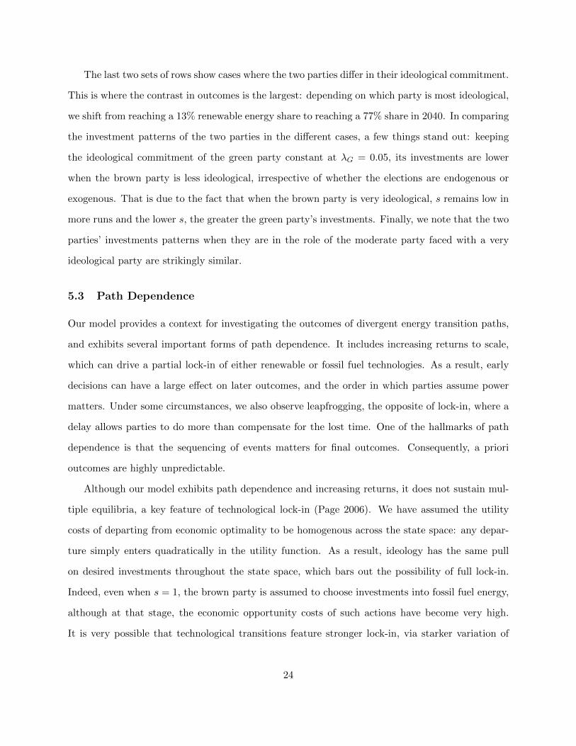
The last two sets of rows show cases where the two parties differ in their ideological commitment.
This is where the contrast in outcomes is the largest: depending on which party is most ideological,
we shift from reaching a 13% renewable energy share to reaching a 77% share in 2040. In comparing
the investment patterns of the two parties in the different cases, a few things stand out: keeping
the ideological commitment of the green party constant at λG = 0.05, its investments are lower
when the brown party is less ideological, irrespective of whether the elections are endogenous or
exogenous. That is due to the fact that when the brown party is very ideological, s remains low in
more runs and the lower s, the greater the green party’s investments. Finally, we note that the two
parties’ investments patterns when they are in the role of the moderate party faced with a very
ideological party are strikingly similar.
5.3 Path Dependence
Our model provides a context for investigating the outcomes of divergent energy transition paths,
and exhibits several important forms of path dependence. It includes increasing returns to scale,
which can drive a partial lock-in of either renewable or fossil fuel technologies. As a result, early
decisions can have a large effect on later outcomes, and the order in which parties assume power
matters. Under some circumstances, we also observe leapfrogging, the opposite of lock-in, where a
delay allows parties to do more than compensate for the lost time. One of the hallmarks of path
dependence is that the sequencing of events matters for final outcomes. Consequently, a priori
outcomes are highly unpredictable.
Although our model exhibits path dependence and increasing returns, it does not sustain mul-
tiple equilibria, a key feature of technological lock-in (Page 2006). We have assumed the utility
costs of departing from economic optimality to be homogenous across the state space: any depar-
ture simply enters quadratically in the utility function. As a result, ideology has the same pull
on desired investments throughout the state space, which bars out the possibility of full lock-in.
Indeed, even when s = 1, the brown party is assumed to choose investments into fossil fuel energy,
although at that stage, the economic opportunity costs of such actions have become very high.
It is very possible that technological transitions feature stronger lock-in, via starker variation of
24

the opportunity costs of pursuing partisan strategies. Thus our following results regarding path
dependence are conservative.
Our model features path dependence in the general sense that outcomes depend on the historical
order of elections (Page 2006). As a measure of path dependence, we compare the outcomes of
different paths at 2040. We consider two measures of path dependence. First, we measure the
variance of s(2040) over paths that have the same count of green electoral terms and take a weighted
average of these variances (where the weights correspond to the frequency of a given count of green
electoral terms in 10,000 runs) to obtain the total variance attributable to sequencing. We denote
this statistic V arseq. Second, we compare the outcome in 2040 (by which time there will be 7
electoral terms), under two radically distinct electoral sequences: GGGBBBB and BBBBGGG.
The results of these two exercises are shown in Figure 10.
[Figure 10 about here.]
The degree of path dependence is heavily influenced by the ideological strength of the parties: for
there to be substantial path dependence, both parties must be strongly ideological. Both statistics
reveal this effect. In the case of equally strong ideological commitment, the change in sequence is
associated with a 15% difference in final outcome, but only 2-8% for the other scenarios.
In the case where both parties are quite ideological, the difference between the GGGBBBB
and BBBBGGG paths is negative: the green party is able to leap-frog renewable energy. This is
because the brown party pursued minor disinvestments during the period when s was low, so that
once the green party had a period of sustained control, it aggressively invested. In contrast, in the
GGGBBBB sequence, any investments in the early period by the green party is undone by vigorous
disinvestments by the ideological brown party.
The analytical structure of the model lends itself to a variety of interesting extensions in future
research. One issue that we have largely omitted is the endogenous growth of the pro-renewables
advocacy coalition. The model could be extended by assuming that renewable energy policies create
endogenous electoral constituencies, and this could further strengthen the logic of path dependence
in the model. In the light of cases such as Germany, where the feed-in tariff has created a strong
25

lobby for renewables (Michaelowa 2005), this extension is certainly worth consideration. In addition,
endogenous electoral constituencies may act as an additional source of path dependence.
A simple way of integrating endogenous electoral preferences in our model is to make λe a
function of s. In other words, as the renewable energy share increases, the weight voters put on
renewables in judging politicians’ energy policy increases. Compared to a baseline in which λe = 0
(voters only care about energy cost), the effect of a growing renewable electoral constituency is to
increase the difference between the policies of the two parties. Indeed, the brown party decreases
its investments as it is additionally induced to keep s low to manage its future electoral advantage.
In opposition, in order to manage its future electoral advantage, the green party increases its
investment policy. The net effect on mean investment paths is zero, and does not increase path
dependence (see A3.5).
6 Conclusion
Human welfare depends on environmental sustainability, and the energy sector is one of the most
important environmental burdens of human activity, contributing to climate change in particular.
The unsustainable nature of contemporary energy use highlights the need for a sustainable energy
transition, but the political feasibility of this phenomenon remains poorly understood. This article
contributes to the debate a general, fully dynamic model with technological learning and endogenous
electoral competition. Building on previous analytical work in energy policy and in other issue areas,
the model allows us to isolate the effects of various political factors, such as partisan polarization
and the intensity of electoral competition on investment in renewable energy.
We begin by contrasting results from a baseline economic model with a cost-minimizing planner
to that with partisan polarization between pro-environment and anti-environment parties. We show
that if the two parties are equally ideological, their behavior has little strategic content. Each party
does move away from the economically optimal strategy for ideological reasons, but neither party
tries to outwit the other by underinvesting or overinvesting in renewables. Asymmetries in the
strength of ideology are required for this kind of behavior. If one of the parties is much more
ideological than the other, dynamic strategies become important. Most importantly, if the green
26
party’s ideological commitment to renewable is strong, perhaps to promote climate mitigation, the
brown party actually appeases by increasing renewable energy investment. The brown party’s goal
is to prevent the green party from making very costly crash investments into renewable energy, and
this can be accomplished through some accommodation.
Endogenizing elections with retrospective or forward-looking voting, we find that the above
results are robust. Moreover, endogenous electoral competition produces additional results impor-
tant for understanding, explaining, and predicting renewable energy policy in our century. Most
importantly, we find that strongly ideological parties are actually more swayed by the electorate’s
preference than more pragmatic parties. Previous studies such as Laver and Sergenti (2011) have
made a crude distinction between ideologically intransigent and pragmatic parties, while we have
found that ideological commitment increases a party’s sensitivity to the preferences of the elec-
torate. This is because highly ideological parties care more about being able to influence policy by
winning elections.
Another natural extension would be to consider variation in national political institutions, such
as the majoritarian-proportional difference. This could prove important if small parties with strong
preferences, such as the Greens, play a pivotal role in winning coalitions. Going beyond the political
logic of renewables, the model could be extended to cover multiple countries. This extension would
allow us to investigate international cooperation, cross-boundary technological spillovers, and policy
diffusion. For example, governments could formulate their renewable energy policies accounting for
the behavior and strategies of their foreign counterparts. Our model could also accommodate the
formation of climate coalitions under a political-economic framework that emphasizes domestic
political institutions and interests.
To our understanding, ours is the first fully dynamic model of energy policy with endogenous
electoral competition. Renewable energy policy is but one example of the different issues that
combine policy-making over long time horizons with intense political competition. Others include
government debt (Alesina and Tabellini 1990), pensions (Jacobs 2011), and fiscal stabilization
(Haggard and Kaufman 1995). Our dynamic approach can be used to shed light on a wide variety
of long-term policy problems in environmental, energy, and other fields of policy. The model marries
27

flexible dynamics with principled behavioral assumptions and, as such, creates opportunities for a
new generation of political-economic models. The computational structure is sufficiently flexible
and accessible to allow social scientists of all stripes to simulate dynamic behavior over long time
horizons, overcoming the limitations of existing analytical models.
28

References
Acemoglu, Daron, Philippe Aghion, Leonardo Bursztyn, and David Hemous. 2012. “The Environ-
ment and Directed Technical Change.” American Economic Review 102 (1): 131–166.
Agnolucci, Paolo. 2007. “Wind Electricity in Denmark: A Survey of Policies, Their Effectiveness
and Factors Motivating Their Introduction.” Renewable and Sustainable Energy Reviews 11 (5):
951–963.
Agnolucci, Paolo. 2008. “Factors Influencing the Likelihood of Regulatory Changes in Renewable
Electricity Policies.” Renewable and Sustainable Energy Reviews 12 (1): 141–161.
Aidt, Toke S. 1998. “Political Internalization of Economic Externalities and Environmental Policy.”
Journal of Public Economics 69 (1): 1–16.
Aklin, Michael, and Johannes Urpelainen. 2013. “Political Competition, Path Dependence, and
the Strategy of Sustainable Energy Transitions.” American Journal of Political Science 57 (3):
643–658.
Alesina, Alberto, and Guido Tabellini. 1990. “A Positive Theory of Fiscal Deficits and Government
Debt.” Review of Economic Studies 57 (3): 403–414.
Camerer, Colin F., Teck-Hua Ho, and Juin-Kuan Chong. 2004. “A Cognitive Hierarchy Model of
Games.” Quarterly Journal of Economics 119 (3): 861–898.
Cederman, Lars-Erik, and Kristian Skrede Gleditsch. 2004. “Conquest and Regime Change: An
Evolutionary Model of the Spread of Democracy and Peace.” International Studies Quarterly 48
(3): 603–629.
Downs, Anthony. 1957. An Economic Theory of Democracy. New York: Harper.
EIA. 2013. “International Energy Outlook.” United States Energy Information Administration.
Enelow, James M., and Melvin J. Hinich. 1984. The Spatial Theory of Voting: An Introduction.
New York: Cambridge University Press.
29
Ferejohn, John A. 1986. “Incumbent Performance and Electoral Control.” Public Choice 50 (1):
5–25.
Fiorina, Morris P. 1981. Retrospective Voting in American National Elections. New Haven: Yale
University Press.
Fischer, Carolyn, and Richard G. Newell. 2008. “Environmental and Technology Policies for Climate
Mitigation.” Journal of Environmental Economics and Management 55 (2): 142–162.
Fuss, Sabine, Jana Szolgayova, Michael Obersteiner, and Mykola Gusti. 2008. “Investment under
Market and Climate Policy Uncertainty.” Applied Energy 85 (8): 708–721.
Golosov, Mikhail, John Hassler, Per Krusell, and Aleh Tsyvinski. 2011. “Optimal Taxes on Fossil
Fuels in General Equilibrium.” NBER Working Paper 17348.
Haggard, Stephan, and Robert R. Kaufman. 1995. The Political Economy of Democratic Transi-
tions. Princeton: Princeton University Press.
Hovi, Jon, Detlef F. Sprinz, and Arild Underdal. 2009. “Implementing Long-Term Climate Policy:
Time Inconsistency, Domestic Politics, International Anarchy.” Global Environmental Politics 9
(3): 20–39.
IEA. 2000. World Energy Outlook. Paris: International Energy Agency.
IEA. 2012. Energy Technology Perspectives 2012: Pathways to a Clean Energy System. Technical
report OECD Publishing. OECD Publishing.
Jacobs, Alan M. 2011. Governing for the Long Term: Democracy and the Politics of Investment.
New York: Cambridge University Press.
Jacobsson, Staffan, and Volkmar Lauber. 2006. “The Politics and Policy of Energy System Trans-
formation: Explaining the German Diffusion of Renewable Energy Technology.” Energy Policy
34 (3): 256–276.
Jamasb, Tooraj. 2007. “Technical Change Theory and Learning Curves: Patterns of Progress in
Electricity Generation Technologies.” Energy Journal 28 (3): 51–71.
30

Laird, Frank N., and Christoph Stefes. 2009. “The Diverging Paths of German and United States
Policies for Renewable Energy: Sources of Difference.” Energy Policy 37 (7): 2619–2629.
Lantz, Eric, Maureen Hand, and Ryan Wiser. 2012. “The Past and Future Cost of Wind Energy.”
National Renewable Energy Laboratory.
Laver, Michael, and Ernest Sergenti. 2011. Party Competition: An Agent-Based Model. Princeton:
Princeton University Press.
List, John A., and Daniel M. Sturm. 2006. “How Elections Matter: Theory and Evidence from
Environmental Policy.” Quarterly Journal of Economics 121 (4): 1249–1281.
Loorbach, Derk. 2010. “Transition Management for Sustainable Development: A Prescriptive,
Complexity-Based Governance Framework.” Governance 23 (1): 161–183.
McCright, Aaron M., and Riley E. Dunlap. 2003. “Defeating Kyoto: The Conservative Movement’s
Impact on U.S. Climate Change Policy.” Social Problems 50 (3): 348–373.
McKibbin, Warwick, Nouriel Roubini, and Jeffrey D. Sachs. 1987. “Dynamic Optimization in
Two-Party Models.” NBER Working Paper 2213.
McNerney, James, J. Doyne Farmer, and Jessika E. Trancik. 2011. “Historical Costs of Coal-fired
Electricity and Implications for the Future.” Energy Policy 39 (6): 3042–3054.
Michaelowa, Axel. 2005. “The German Wind Energy Lobby: How to Promote Costly Technological
Change Successfully.” European Environment 15 (3): 192–199.
Moe, Terry M. 2005. “Power and Political Institutions.” Perspectives on Politics 3 (2): 215–233.
Nemet, Gregory F. 2006. “Beyond the Learning Curve: Factors Influencing Cost Reductions in
Photovoltaics.” Energy Policy 34 (17): 3218–3232.
Neumayer, Eric. 2003. “Are Left-Wing Party Strength and Corporatism Good for the Environment?
Evidence from Panel Analysis of Air Pollution in OECD Countries.” Ecological Economics 45
(2): 203–220.
31

Page, Scott E. 2006. “Path Dependence.” Quarterly Journal of Political Science 1 (1): 87–115.
Russel, Duncan, and David Benson. 2013. “Green Budgeting in an Age of Austerity: A Transat-
lantic Comparative Perspective.” Environmental Politics 23 (2): 243–262.
Schelling, Thomas C. 1960. The Strategy of Conflict. Cambridge: Harvard University Press.
Schwoon, Malte. 2006. “Simulating the Adoption of Fuel Cell Vehicles.” Journal of Evolutionary
Economics 16 (4): 435–472.
Shipan, Charles R., and William R. Lowry. 2001. “Environmental Policy and Party Divergence in
Congress.” Political Research Quarterly 54 (2): 245–263.
Shum, Kwok L., and Chihiro Watanabe. 2007. “Photovoltaic Deployment Strategy in Japan and
the USA.” Energy Policy 35 (2): 1186–1195.
Smith, Adrian, Florian Kern, Rob Raven, and Bram Verhees. 2014. “Spaces for Sustainable Inno-
vation: Solar Photovoltaic Electricity in the UK.” Technological Forecasting and Social Change
81: 115–130.
Toke, David, and Volkmar Lauber. 2007. “Anglo-Saxon and German Approaches to Neoliberalism
and Environmental Policy: The Case of Financing Renewable Energy.” Geoforum 38 (4): 677–
687.
Torvanger, Asbjorn, and James Meadowcroft. 2011. “The Political Economy of Technology Support:
Making Decisions About Carbon Capture and Storage and Low Carbon Energy Technologies.”
Global Environmental Change 21 (2): 303–312.
Ulmanen, Johanna H., Geert P.J. Verbon, and Rob P.J.M. Raven. 2009. “Biofuel Developments in
Sweden and the Netherlands: Protection and Socio-Technical Change in a Long-Term Perspec-
tive.” Renewable and Sustainable Energy Reviews 13 (6-7): 1406–1417.
Unruh, Gregory C. 2000. “Understanding Carbon Lock-In.” Energy Policy 28 (12): 817–830.
Urpelainen, Johannes. 2012. “Global Warming, Irreversibility, and Uncertainty: A Political Anal-
ysis.” Global Environmental Politics 12 (4): 68–85.
32
Verbong, Geert, and Frank Geels. 2007. “The Ongoing Energy Transition: Lessons from a Socio-
Technical, Multi-Level Analysis of the Dutch Electricity System (1960-2004).” Energy Policy 35
(2): 1025–1037.
Victor, David G. 2011. Global Warming Gridlock: Creating More Effective Strategies for Protecting
the Planet. New York: Cambridge University Press.
Walz, Rainer. 2007. “The Role of Regulation for Sustainable Infrastructure Innovations: The Case
of Wind Energy.” International Journal of Public Policy 2 (1-2): 57–88.
33
2015 2020 2025 2030 2035 2040 2045 2050 2055 20600
0.1
0.2
0.3
0.4
0.5
$1000/TJ
$1556/TJ
$2111/TJ
$2667/TJ
$3222/TJ$3778/TJ$6000/TJ
Year
Ren
ewab
le e
nerg
y sh
are
(s)
(a) The evolution over time of the renewable energy share, under constant fuel prices, as a function of fuelprices.
0 0.1 0.2 0.3 0.4 0.5 0.6 0.7 0.8 0.9 10
0.002
0.004
0.006
0.008
0.01
0.012
0.014
0.016
Renewable Energy Share
Inve
stm
ents
(%
of Q
)
Fuel price ($/TJ)
1000
1500
2000
2500
3000
3500
4000
4500
5000
5500
6000
(b) Optimal economic investment as a function of the renewable energy share and fuel price in the absenceof a trend in the fuel price. The optimal investments do not change over the 50-year time scale of interestin the subsequent analyses.
Figure 1: Characteristics of the economic optimum, in the absence of a trend in the fuel price.
34

0 0.1 0.2 0.3 0.4 0.5 0.6 0.7 0.8 0.9 1−0.08
−0.06
−0.04
−0.02
0
0.02
0.04
0.06
0.08
Renewable energy share (s)
Inve
stm
ents
(q,
% o
f Q)
λ
0.02
0.03
0.04
0.05
0.06
0.07
0.08
Figure 2: Investment strategies of both parties, for increasing values of λ, for a fuel price of $3000/TJ(at t=2). The dashed line denotes the economically optimal strategy. Green party investments lieabove this, and brown party investment lie below it.
35

0 0.1 0.2 0.3 0.4 0.5 0.6 0.7 0.8 0.9 1−0.01
0
0.01
0.02
0.03
0.04
0.05
0.06
0.07
0.08
Renewable energy share (s)
Inve
stm
ents
(q,
% o
f Q)
λ
0.02
0.03
0.04
0.05
0.06
0.07
0.08
Figure 3: Investment strategies of both parties, for increasing values of λG while keeping λB constantat 0.01, for a fuel price of $3000/TJ (at t=2).
36

0 0.2 0.4 0.6 0.8 1−0.1
−0.05
0
0.05
0.1
Inve
stm
ents
(q)
λ =0.010
0 0.2 0.4 0.6 0.8 1−0.1
−0.05
0
0.05
0.1λ =0.030
0 0.2 0.4 0.6 0.8 1−0.1
−0.05
0
0.05
0.1
Renewable energy share (s)
Inve
stm
ents
(q)
λ =0.050
0 0.2 0.4 0.6 0.8 1−0.1
−0.05
0
0.05
0.1
Renewable energy share (s)
λ =0.070
p
0
0.1
0.2
0.3
0.4
0.5
0.6
0.7
0.8
0.9
1
Figure 4: Investment strategies of both parties, for increasing values of λ = λG = λB, for a fuelprice of $3000/TJ and in period T=5.
37

0 0.2 0.4 0.6 0.8 1−0.1
−0.05
0
0.05
0.1
Inve
stm
ents
(q)
λ =0.010
0 0.2 0.4 0.6 0.8 1−0.1
−0.05
0
0.05
0.1λ =0.030
0 0.2 0.4 0.6 0.8 1−0.1
−0.05
0
0.05
0.1
Renewable energy share (s)
Inve
stm
ents
(q)
λ =0.050
0 0.2 0.4 0.6 0.8 1−0.1
−0.05
0
0.05
0.1
Renewable energy share (s)
λ =0.070
p
0
0.1
0.2
0.3
0.4
0.5
0.6
0.7
0.8
0.9
1
Figure 5: Investment strategies of both parties with fixed λB = 0.01 and λG increasing for a fuelprice of $3000/TJ and in period T=5.
38

−0.2 −0.1 0 0.1 0.2
0.35
0.4
0.45
0.5
0.55
0.6
0.65
0.7
∆
p
b=0.5
b=0.4
b=0.3
0 0.2 0.4 0.6 0.8 1−0.06
−0.04
−0.02
0
0.02
0.04
0.06
0.08
0.1
Renewable energy share (s)
Ele
ctor
ate
inve
stm
ent p
ref (
q*e)
λe
0
0.05
0.1
0.15
0.2
0.25
Figure 6: First panel: Shape of the aggregate election response function given by equation 8.Since (−0.2, 0.2) is the range of possible disagreements over the action variable q, the responsefunction is plotted on that range. Second panel: Preferred actions of the electorate for varyingvalues of λe, compared to the present preference of parties for λi = 0.06 (dashed lines).
39
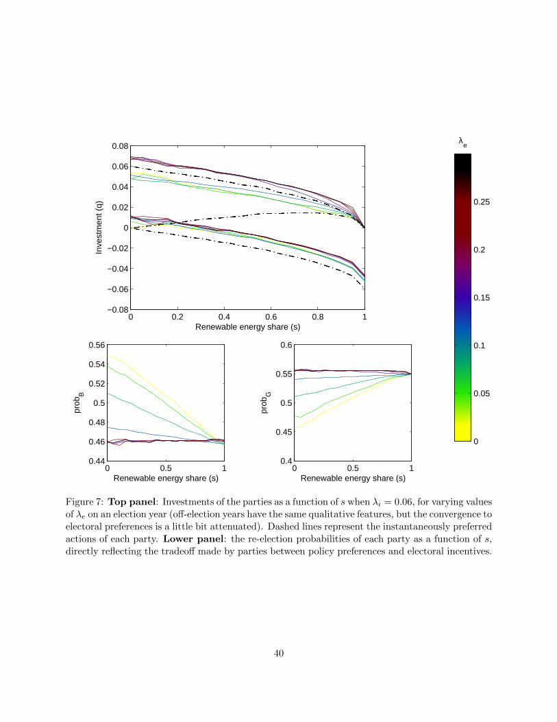
0 0.2 0.4 0.6 0.8 1−0.08
−0.06
−0.04
−0.02
0
0.02
0.04
0.06
0.08
Renewable energy share (s)
Inve
stm
ent (
q)
0 0.5 10.44
0.46
0.48
0.5
0.52
0.54
0.56
Renewable energy share (s)
prob
B
0 0.5 10.4
0.45
0.5
0.55
0.6
Renewable energy share (s)
prob
G
λe
0
0.05
0.1
0.15
0.2
0.25
Figure 7: Top panel: Investments of the parties as a function of s when λi = 0.06, for varying valuesof λe on an election year (off-election years have the same qualitative features, but the convergence toelectoral preferences is a little bit attenuated). Dashed lines represent the instantaneously preferredactions of each party. Lower panel: the re-election probabilities of each party as a function of s,directly reflecting the tradeoff made by parties between policy preferences and electoral incentives.
40
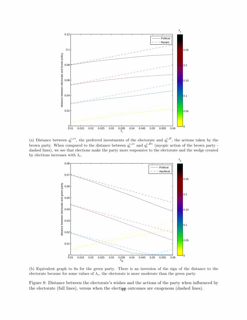
0.01 0.015 0.02 0.025 0.03 0.035 0.04 0.045 0.05 0.055 0.060
0.02
0.04
0.06
0.08
0.1
0.12
λi
dist
ance
bet
wee
n el
ecto
rate
and
bro
wn
polic
y
Political
Myopic
λe
0
0.05
0.1
0.15
0.2
0.25
(a) Distance between qc,e∗t , the preferred investments of the electorate and qc,Bt , the actions taken by the
brown party. When compared to the distance between qc,e∗t and qc,B∗t (myopic action of the brown party -
dashed lines), we see that elections make the party more responsive to the electorate and the wedge createdby elections increases with λi.
0.01 0.015 0.02 0.025 0.03 0.035 0.04 0.045 0.05 0.055 0.060
0.01
0.02
0.03
0.04
0.05
0.06
0.07
0.08
λB
dist
ance
bet
wee
n el
ecto
rate
and
gre
en p
arty
Political
Apolitical
λe
0
0.05
0.1
0.15
0.2
0.25
(b) Equivalent graph to 8a for the green party. There is an inversion of the sign of the distance to theelectorate because for some values of λe, the electorate is more moderate than the green party.
Figure 8: Distance between the electorate’s wishes and the actions of the party when influenced bythe electorate (full lines), versus when the election outcomes are exogenous (dashed lines).41

(a) Baseline economic model and the exogenous elections under two different sets of ideological parameters.
(b) Endogenous elections with strongly ideological parties (λG = λB = 0.05) and varying preferences of theelectorate.
Figure 9: Mean and standard deviation of 10, 000 simulations of the transition for the economicmodel and the two different political models.
42
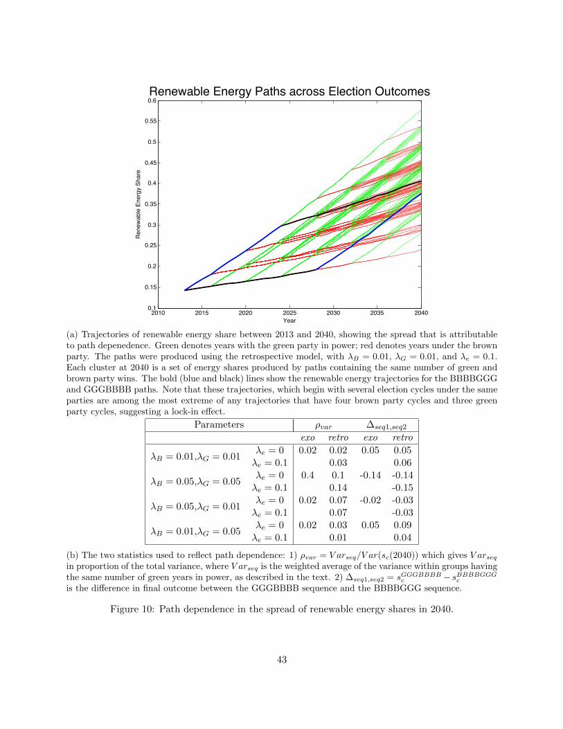
2010 2015 2020 2025 2030 2035 20400.1
0.15
0.2
0.25
0.3
0.35
0.4
0.45
0.5
0.55
0.6Renewable Energy Paths across Election Outcomes
Year
Ren
ewab
le E
nerg
y Sh
are
(a) Trajectories of renewable energy share between 2013 and 2040, showing the spread that is attributableto path depenedence. Green denotes years with the green party in power; red denotes years under the brownparty. The paths were produced using the retrospective model, with λB = 0.01, λG = 0.01, and λe = 0.1.Each cluster at 2040 is a set of energy shares produced by paths containing the same number of green andbrown party wins. The bold (blue and black) lines show the renewable energy trajectories for the BBBBGGGand GGGBBBB paths. Note that these trajectories, which begin with several election cycles under the sameparties are among the most extreme of any trajectories that have four brown party cycles and three greenparty cycles, suggesting a lock-in effect.
Parameters ρvar ∆seq1,seq2
exo retro exo retro
λB = 0.01,λG = 0.01λe = 0 0.02 0.02 0.05 0.05λe = 0.1 0.03 0.06
λB = 0.05,λG = 0.05λe = 0 0.4 0.1 -0.14 -0.14λe = 0.1 0.14 -0.15
λB = 0.05,λG = 0.01λe = 0 0.02 0.07 -0.02 -0.03λe = 0.1 0.07 -0.03
λB = 0.01,λG = 0.05λe = 0 0.02 0.03 0.05 0.09λe = 0.1 0.01 0.04
(b) The two statistics used to reflect path dependence: 1) ρvar = V arseq/V ar(sc(2040)) which gives V arseqin proportion of the total variance, where V arseq is the weighted average of the variance within groups havingthe same number of green years in power, as described in the text. 2) ∆seq1,seq2 = sGGGBBBB
c − sBBBBGGGc
is the difference in final outcome between the GGGBBBB sequence and the BBBBGGG sequence.
Figure 10: Path dependence in the spread of renewable energy shares in 2040.
43
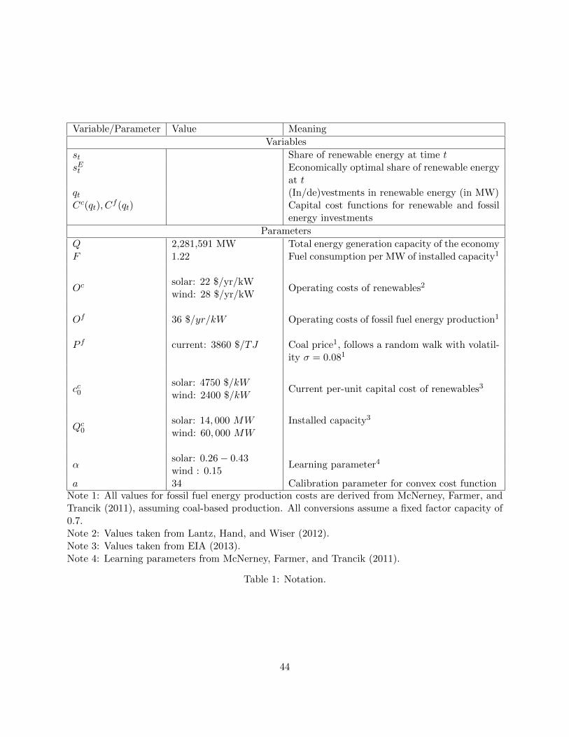
Variable/Parameter Value Meaning
Variables
st Share of renewable energy at time tsEt Economically optimal share of renewable energy
at tqt (In/de)vestments in renewable energy (in MW)Cc(qt), C
f (qt) Capital cost functions for renewable and fossilenergy investments
Parameters
Q 2,281,591 MW Total energy generation capacity of the economyF 1.22 Fuel consumption per MW of installed capacity1
Ocsolar: 22 $/yr/kW
Operating costs of renewables2wind: 28 $/yr/kW
Of 36 $/yr/kW Operating costs of fossil fuel energy production1
P f current: 3860 $/TJ Coal price1, follows a random walk with volatil-ity σ = 0.081
cc0solar: 4750 $/kW
Current per-unit capital cost of renewables3wind: 2400 $/kW
Qc0solar: 14, 000 MW Installed capacity3
wind: 60, 000 MW
αsolar: 0.26− 0.43
Learning parameter4wind : 0.15
a 34 Calibration parameter for convex cost functionNote 1: All values for fossil fuel energy production costs are derived from McNerney, Farmer, andTrancik (2011), assuming coal-based production. All conversions assume a fixed factor capacity of0.7.Note 2: Values taken from Lantz, Hand, and Wiser (2012).Note 3: Values taken from EIA (2013).Note 4: Learning parameters from McNerney, Farmer, and Trancik (2011).
Table 1: Notation.
44

Parameters sc(2040) qB qC green wins %exo retro exo retro exo retro exo retro
λB = 0.01,λG = 0.01λe = 0 0.373 0.374(0.06) 0.006 0.005(0.001) 0.016 0.015(5e−4) 50 49.5(13.9)λe = 0.1 0.382(0.06) 0.006(0.001) 0.016(5e−4) 50.7(13.8)
λB = 0.05,λG = 0.05λe = 0 0.540 0.520(0.178) −0.010 −0.013(0.005) 0.040 0.035(0.005) 49.7 50(14.8)λe = 0.1 0.627(0.163) −0.012(0.006) 0.033(0.005) 54.5(13.9)
λB = 0.05,λG = 0.01λe = 0 0.134 0.132(0.052) −0.007 −0.006(0.001) 0.007 0.007(7e−4) 50 50.3(0.14)λe = 0.1 0.130(0.056) −0.006(0.001) 0.008(8e−4) 51.25(13.9)
λB = 0.01,λG = 0.05λe = 0 0.771 0.760(0.101) 0.007 0.007(0.003) 0.028 0.025(0.005) 49.8 48.9(0.14)λe = 0.1 0.790(0.079) 0.008(0.003) 0.024(0.004) 51.6(0.14)
Table 2: Mean and standard deviation of outcomes in 2040, investments by the brown and greenparty and election outcomes.
45