path integration on the hyperbolic plane with a magnetic …€¦ · · 2007-03-09path...

ANNALS OF PHYSICS 201, 258-284 (1990)

Path Integration on the Hyperbolic Plane with a Magnetic Field

CHRISTIAN GROSCHE*

II, Institut ftir Theoretische Physik, Universitiit Hamburg, Luruper Chaussee 149, 2000 Hamburg 50, Federal Republic of Germany

Received August 29, 1989

In this paper I discuss the path integrals on three formulations of hyperbolic geometry, where a constant magnetic field B is included. These are: the pseudosphere /i’, the Poincare disc D, and the hyperbolic strip S. The corresponding path integrals can be reformulated in terms of the path integral for the modified PBschl-Teller potential. The wave-functions and the energy spectrum for the discrete and continuous part of the spectrum are explicitly calculated in each case. First the results are compared for the limit B+ 0 with previous calculations and second with the path integration on the Poincare upper half-plane U. This work is a continuation of the path integral calculations for the free motion on the various formulations on the hyperbolic plane and for the case of constant magnetic field on the Poincart upper half-plane U. 0 1990 Academic Press. Inc.

I. INTRODUCTION

The technique of calculating path integrals explicitly has improved remarkable in the last 10 years. Since the invention of the path integral by Feynman [ 151 there has only been available the solution of the harmonic oscillator (or to be precise, the general quadratic Lagrangian [44]) and its special cases, the free particle, of course, included. A formulation in general coordinates, i.e., on curved manifolds, was first given by Dewitt [ 111, followed by several discussions refining and improving the path integral calculus, e.g., by McLaughlin and Schulman [35], Mizrahi [36], Gervais and Jevicki [17], Omote [37], Marinov [34], T. D. Lee [ 321 and later on by Grosche and Steiner [24].

The formulation of path integrals in polar coordinates by Arthurs [ 11, Peak and Inomata [40], Goovaerts [18], Steiner [47], and Grosche and Steiner [24] opened new possibilities in discussing path integral problems which can be reformulated in terms of the radial harmonic oscillator. Here a new technique originally developed by Duru and Kleinert [ 131 in their treatment of the hydrogen atom could be applied in its full power. The main idea in these “space-time” trans-

* Supported by Deutsche Forschungsgemeinschaft under contract DFG-Mu 757/2-3. Present address: The Blockett Laboratory, Imperial College of Science, Technology and Medicine, Prince Consort Road, London SW7 2BZ, UK.

0003-4916/90 $7.50 Copyright 0 1990 by Academic Press, Inc. All rights of reproduction in any form reserved.

258

PATH INTEGRATION ON HYPERBOLIC GEOMETRY 259

formations of path integrals is that a problem which is not tractable in its original coordinates can be made tractable in a new coordinate system, where in addition a non-linear transformation of the “old” time T into the “new time” s” must be performed. In fact, one uses specific symmetry properties of the problem in question to perform this combined “space-time” transformation.

But not all problems possess the symmetry properties of the radial harmonic oscillator which in fact are all variations of problems which lead on the operator level to confluent hypergeometric functions (with Hermite- and Laguerre- polynomials, Bessel- and Whittaker-functions, respectively). Another type of solvable problems in quantum mechanics is closely related to the hypergeometric function (Legendre-polynomials and -functions, Gegenbauer- and Jacobi- polynomials) and can be set in relation with the (modified) PGschl-Teller potential. The “hidden” symmetry properties in these potential problems are the SU(2) and SU( 1, 1) symmetries, respectively.

In this paper I want to continue previous work on path integrals on the hyperbolic plane which can be formulated in various coordinates systems.

(1) To discuss this in some detail let us start with the pseudasphere A* which is defined by

A2 := (bw*,Y3)1 -y:+y:+y:= -1). (1)

A2 can be visualized as a hyperboloid embedded in R3 [4]. But be careful: A2 has negative Gaussian curvature K = - 1, i.e., it is everywhere saddle-shaped. A more convenient description for ,4* reads in pseudospherical polar coordinates (z, 4) [4,49, 501:

y, =cosh z, y, = sinh z cos 4, y, = sinh z sin 4 (z 3 094 E LO, 2x1). (2)

The metric g, associated with the line element ds2 =gObdgodqh reads g,b = diag( 1, sinh* 5).

(2) With the stereographic projection of A2 onto the complex (x,, x,)-plane we get the Poincart! disc D:

z=x,+ix,=re’~=‘~=tanh~(sin(+icosI). 1 +Yl

Here the metric reads g,b = [2/( 1 - r’)]’ diag( 1, r*).

(3) The Poincari: disc D can be mapped onto the Poincark upper half-plane U by the Cayley-transformation:

The metric reads g,, = l/y*. 6,b. (4) With the help of the transformation

q=X+iY= -ln(-ii) (= 2 arctanh z), (5)

260 CHRISTIAN GROSCHE

we can finally map the Poincart upper half-plane (the Poincart disc) onto the hyperbolic strip S. Here the metric reads g,, = l/cos2 Y. a,,.

The hyperbolic distance r = d(p”, p’) [p - any of the coordinates (r, d), (xi, x2), (x, y), (X, Y)] in these spaces is given by

cash r = cash z” cash z’ - sinh Z” sinh r’ cos(#” - 4’) (on A2)

(on D)

(6) (on u)

cosh(X” -X) = cos y’ cos Y

-tan Y tan Y (on S).

Recently these models for a non-Euclidean geometry have become important in the theory of strings, in particular in the Polyakov approach for the bosonic string (see, e.g., [20,41]), in the theory of quantum chaos and periodic orbit theory see [4,28,46,48]), and for non-Euclidean harmonic analysis [49]. In string perturbation theory one considers open or closed Riemannian surfaces of genus g, where the order of the perturbation expansion corresponds to g. For a closed Riemannian surface one has, e.g., for g = 1 the torus and for g = 2 the double doughnut. These surfaces are conformally equivalent to compact domains (polygons) with 4g edges and vertices in these Riemannian spaces (e.g., for g = 2 an octagon in D, say). Furthermore, these compact domains are fundamental domains of discrete sub- groups of PSL(2, R) [29]. The action of the group elements are for, e.g., z E D,

az + b ZH

a* + b*z (/al’- lb12= 1)

which are isometries in D. Under the action of the generators of the group the polygons tessalate D, say, where PSL(2, R) is in fact the group SU( 1, 1). The periodic orbit theory in this case leads to the Selberg trace formula [29,45].

However, I do not consider the motion in bounded domains; for an attempt to calculate energy levels and wave-fucntions in bounded domains in D see Aurich, Sieber, and Steiner [2] and Aurich and Steiner [3].

In some recent publications we have studied the path integral formulations on the Poincare upper half-plane U [25], the d-dimension1 pseudosphere Ad- ’ [26] and on the Poincart disc D and on the hyperbolic strip S [23]. Further contributions are due to Biihm and Junker [8], Gutzwiller [28] and Kubo [31]. In these papers the free motion has been studied. However, the path integral treatment including a (constant) magnetic field is more involved. The path integral treatment on U including such a magnetic field was discussed in Ref. [22]. In the present paper these discussions are completed for all the various formulations of hyperbolic geometry (the hyperbolic plane), i.e., I discuss the path integrals on the Pseudo-


sphere /1’, on the Poincare disc D and on the hyperbolic strip S including a magnetic field. The purpose is to give further contributions to an alternative complete description building up quantum mechanics from the point of view of fluctuating paths, i.e., path integrals [ 131.

A discussion of /1* with a magnetic field is due to Oshima [38]. This author expanded, using results of Fay [ 141, the short-time kernel in terms of the eigen- functions of the corresponding Schrijdinger operator and exploited in each jth-step of the path integration the known completeness and orthogonality relations of the eigen-functions. Thus the calculation becomes trivial. But this procedure seems somewhat unsatisfactory because this is possible in every path integral problem, if one knows the solution from the operator formalism, and does nor solve the problem of calculating a path integral explicitly in an operator independent manner.

However, in the present paper the path integrals in these spaces /1*, D, and S are calculated starting in their original coordinates. By Fourier expansion (and if needed an appropriate coordinate transformation) in each case the path integral of a modified Poschl-Teller potential is obtained. Using the results of this path integral problem (see below) the original problems can be solved successfully.

In constructing the path integrals on A*, D, and S with a magnetic field the “product-ordering” prescription is used as discussed in Ref. [21]. Let us summarize the most important features of this prescription which must be only slightly modified in the cases here to include the magnetic terms. We start with the generic case, i.e., the classical Lagrangian and Hamiltonian is given by

We rewrite the metric tensor g,, in the form (which under reasonable assumptions is always possible, e.g., positive definite scalar product)

gab(q) = i L(q) h,,(q) (9)

(d= dimension of the Riemannian manifold). The quantum Hamiltonian is constructed in the usual way by the Laplace-Beltrami operator d,, (e.g., [36], we use units fi = 1; in the following sums over repeated indices are understood):

(10)

(g = determinant of the metric tensor gab). We introduce momentum operators

P, = - W, + r,/2), r,=d,ln&. (11)


Rewriting the Hamiltonian (10) in terms of the momentum operators pa we choose a product ordering prescription,

with the well-defined quantum correction AF’ given by (h := det(h,) =&):

4hachbc,ab + 2hnchbc +‘+ 2h”’ hbc,b h hb f + hbc,a L

h > _ ho“j+‘C &c&b 1 h2 *

(13)

In the formulation of Eq. (12) we have assumed for simplicity that for the vector- potential we have A, = A,(qb) (b # a), which means that the &h-component of the vector-potentials does not depend on the ath-coordinate. This will be sufficient for our purposes. In the general case for arbitrary vector potential A, it is simpler to use the midpoint prescription in the path integral and evaluate A(q) at A(q”‘) = A[.L(~W + q(j- 1) )] or at A(q”‘) = t[A(q(j- “) + A(q”))] , respectively. See, e.g., [36,44].

There is an important special case of Eq. (13). Let us assume that g,, is propor- tional to the unit tensor, i.e., g,b = A *dab. Then A V simplifies into

AV=$ [(4-d)A;+2A~A,,]. (14)

This implies that if d = 2 the quantum potential A V vanishes! Using the Trotter formula e-“(A+B) = s - lim,, u3 (e-“A’Ne-itB”“)N and the

short-time approximation for the matrix element (q” 1 e-i’H 1 q’ ) one obtains in the usual manner the Lagrangian path integral in the “product form” definition [Aq(A = qU) _ qtj- 1) ,q”‘=q(t”‘), t”‘=t’+j~, j=l,...,N, &=T/N=(t”-t’)/N,

N + co, j22) =f(q(j- ‘I) f(q”‘), f any function of the coordinates]:

Wq”, 4’; 0

(15)


The expression in square brackets is nothing but the classical Lagrangian with an additional quantum correction potential A V: Y& = &, - A V. Clearly, one has to prove that with the short time kernel of this path integral the time-dependent Schrodinger equation

(16)

can be derived via the time evolution equation

$(q”; ,,,I = J” &a K(q”, 4’; T) Nq’; t’) 4’. (17)

This is in fact the case-see [21]. For successfully solving the various path integrals in this paper we need the path

integral solution of the modified Poschl-Teller (mPT) potential pPT. The modified Poschl-Teller potential with some numbers r] and v is defined as

drl-1) v(v-1) x---- cash’ r 1 (r > 0). (18)

This kind of potentials get their name from the original work of Poschl and Teller 1421, where the hyperbolics are replaced by the usual trigonometric functions, so that the Pbschl-Teller potential has a “hidden” SU(2) symmetry. A classical study of this problem is due to Frank and Wolf [16]: The path integral problem for the SU(2) manifold was discussed by Duru [ 123 and Bijhm and Junker [S], whereas the SU( 1, 1) problem was discussed by Biihm and Junker [7, 81. The special case v(v - 1) = 0 can be studied with the help of the path integral on the pseudosphere [26]. Some care is needed in the path integral formulation for the modified Pbschl-Teller potential. Looking carefully at the lattice derivation [7, 81 for the path integral we see that we must use a functional measure formulation similar to the one used in the lattice formulation for the radial harmonic oscillator [24,40,47]. This has the consequence that the following interpretation scheme must be used, namely

KmPT(r”, r’; T)

= Dr(r)p,,.[sinhr,coshr]exp(Tjt:i2dr) s

= lim N- ot, (&)N’2 zc,’ j: dr(j)j, p,,,[sinh r(l), cash r”‘j

[

im x exp 2E (,(A - #- 1 I)* , 1 (19)


where the functional measure ps,” is given by

pV.,[sinh r, cash r]

= lim fi pq,,[sinh r(j), cash r(j)] N-cc.

J=1

(20)

The first line in Eq. (19) has only the symbolic meaning that formally the potential appearing in the Schrodinger equation translates into j Dx exp(i x Action). We emphasize that only the functional measure formulation has a well-defined lattice formulation. The usual expansion of the modified Bessel function Z,(z) N (27t~)-‘/~ exp[z - (v2 - l/4)/22] [z + co, arg(z) # 0] (or Eq. (3.15) in Ref. [30], respectively) seems very suggestive but gives in the lattice formulation the wrong boundary behaviour of the corresponding short-time kernels and wave-functions because the condition arg(z) # 0 is violated. Instead of the correct behaviour we would get a highly singular one. But it is not the scope of this paper to discuss these features in detail; this will be done elsewhere [27]. Adopting the notation of Frank and Wolf the path integral solution reads [define 2s = q(r~ - 1 ), - 2c = v(v - 1) and introduce the numbers k,, k2 which are defined in terms of c and s as k, =

$(1&/m), k2=f(lf,/m)]:

Here NM denotes the maximal number of states with 0, 1, . . . . n < N, <k, - kz - f. The correct signs depend on the boundary conditions for r -+ 0 and r + co, respectively. In particular one gets for s = 0 an even and an odd wave-function corresponding to k, = 4, z, respectively. The bound states are explicitly given by

‘JJI((1*k2)(r) = NLkI, kZ)(sinh r)2k2- l/2 (cosh r)-2kl + 3/2

xzF,(-k,+k2+~, -kI+k2-K+1;2k2; -sinh2r), Wa)


2n!(2k, - 1) Q2k, -n - 1) 1’2 = r(2k, + n) f(2k, - 2k, - n) 1

x (sinh r)2kZ-“2 (cash Y) - 2n Zk,+3/2p[2k2-1.2(k,-kkz-n)-1] n

1 N(h, h) = - (2k,-l)T(k,+k,-k)T(k,+k,+ic-1) I” n

Wk,) 1 T(k,-k,+rc)T(k,-k,-K+l) ’

Pb)

PC)

(23)

The continuous states read

yFlrk2)(y) = N~kl,k2)(cosh r)Zkl- 112 (sinh r)2k2- l/Z

x ?F,(k, + k, - K, k, + k, + K - 1; 2k,; - sinh2 r), Wa)

x[T(k,+k,-rc)r(-k,+k,+ti)

xT(k,+k2+k.-l)I’(-kl+k2-K+l)]1’2, Pb)

where K = 4( 1 + ip) (k > 0) and E = p2/2m. In the formulation of the path integrals on A”, D, and S with a magnetic field

we start from the formulation given in the coordinates of the Poincare upper half- plane U [9, lo]:

where the vector potential is given by

(26)

The specific choice of the vector potential is not unique. By a gauge transformation it can be changed leaving the magnetic field unaltered. Introducing an arbitrary two-dimensional coordinate system (x,y) the magnetic fields described by the two-form B = dA = (a,,A, - a,A,) dx A dy. B is unaltered by the change A -+ A’ = A +VF, where F= F(x, y) is some arbitrary function FE C2( { (x, y)}) H R. Making the ansatz (with the same restrictions on A as above)

a=~h”‘(y)(p,+~d,)(p,+~A,)h6’(y)+ V(q)+dV(q) (27)


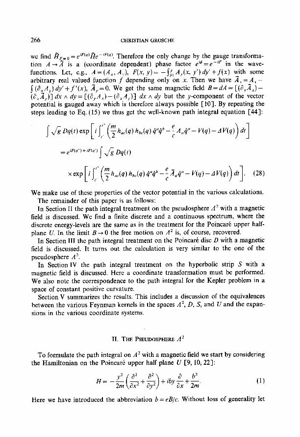
we find AFE-O=eiF(we- . jFCq) Therefore the only change by the gauge transformation A + A” is a (coordinate dependent) phase factor e” = e-jF in the wave- functions. Let, e.g., A = (A,, A,), F(x, v) = - jJO A,(x, y’) dy’ +f(x) with some arbitrary real valued function f depending only on x. Then we have A”, = A,- f (L4,) dy’ + f ‘(x), A”,, = 0. w e get the same magnetic field B = d4 = [(d,A,) -

(&A”,)1 dx A 4 = CGQ,) - @xA,Jl d x A dy but the y-component of the vector potential is gauged away which is therefore always possible [lo]. By repeating the steps leading to Eq. (15) we thus get the well-known path integral equation [44]:

ih,,(q)h,,(q)4”4b-~A,4”- v(q)--df’(q) dt > 1 = eiF(q”) + iF(q’)

We make use of these properties of the vector potential in the various calculations. The remainder of this paper is as follows: In Section II the path integral treatment on the pseudosphere A* with a magnetic

field is discussed. We find a finite discrete and a continuous spectrum, where the discrete energy-levels are the same as in the treatment for the Poincart upper half- plane U. In the limit B -+ 0 the free motion on A* is, of course, recovered.

In Section III the path integral treatment on the Poincare disc D with a magnetic field is discussed. It turns out the calculation is very similar to the one of the pseudosphere A*.

In Section IV the path integral treatment on the hyperbolic strip S with a magnetic field is discussed. Here a coordinate transformation must be performed. We also note the correspondence to the path integral for the Kepler problem in a space of constant positive curvature.

Section V summarizes the results. This includes a discussion of the equivalences between the various Feynman kernels in the spaces A*, D, S, and U and the expan- sions in the various coordinate systems.

II. THE PSEUDOSPHERE A2

To formulate the path integral on A* with a magnetic field we start by considering the Hamiltonian on the Poincart upper half plane U [9, 10,221:

Here we have introduced the abbreviation b = eB/c. Without loss of generality let


us assume that b > 0. A direct transformation of variables U + ,4’ gives a Hamiltonian on A2 which is very complicated and in fact of no use. Let us introduce complex variables on U as z =x + i-v and define r(i, co) and e(i, co) by

’ - To tanh r(c7 Co) e-l&;, io) i-i0 2 3 (2)

where r(i, co) is in fact the PSL(2, R)-invariant hyperbolic distance of Eq. (1.6). For co = i we have the following relation with the coordinates on A2 : r([, i) = r and 19({, i)=#+n/2 [cf. Eq. (I.3)]. Let us now construct the PSL(2, R) invariant Hamiltonian on U with an arbitrary co E U [ 141:

=v[-&$+b(&$+&$)

b2 (Co-ib)(i-0 b2 (i-~oo)(io-o+2m

a = ar2i2 i )+coth r(L Co)- 1 a2 2 0 WL lo) ’ sinh’ r(i, lo) ae2K, Co)

2 a + 1+ cash r([, Co)

b2+ibaofi, ro) -b2 > 1 .

(3)

(4)

Choosing to = i we get for Hb(i, co) in the coordinates on U, A*, and D, respectively

-b2 NC-1) (i+i)(i-[)+b2 1 (on u) (5)

= -LJkp($ +fg+f$)+(l-r’)(b’+ib$)-b’]

(OnD). (7)


The two Hamiltonians on /i2 and D are appropriate for our purposes. In this section we consider only A*. Introducing the momentum operators

p,=$” z a& (8)

which are hermitian with respect to the scalar product

sinh r dz Y,(z, 4) Y’:(z, 4) cy'1, ~2E~2(‘42n (9)

we rewrite the Hamiltonian (6) yielding

Here the vector-potential A is given by

A= 0

=B(coshz-1) 1 . 0

(11)

The magnetic field is thus calculated to read as dB = (d,A, - arAT) dT A dq3 = (m/2) B sinh r dz A dd which has the form constant x volume-form and can therefore be interpreted as a constant field on A*. The classical Lagrangian and Hamiltonian are given by

9;: = 5 (f’ + sinh2 rd2) - b(cosh 7 - 1) 4,

(12)

Constructing the path integral for ,4* we follow the prescription given in the Intro- duction and get

Icqz", 7', I$", (8'; T)

= s sinh 7 Dz(t) D#(t)


N

(I (

n xexp i 1 ,= 1 E (A*r”’ + sinh* r(j)d2q5(j’

>

- b(co~~~’ - 1) A#“’ - 8m siTh2 T(j))]. (13)

We perform a Fourier expansion according to

This gives for K$:

K&z”, r’; T)

exp( - iT/8m) = 27c

liyw (&)” >: j: sinh ,(j)dT”’

N

x n exp j=l lE

8m sinh’ z(j)

=&exp[ -g(b’+t)]

x (sinh z’ sinh ,“)-l’* lim &‘-.a (G)N’2 jj,‘f; dr”’

ANT-- E 2;?-;;itcj, -; 1 :ro;;;cj,)]

=&exp[ -$(b’+t)l

x (sinh T’ sinh t”)- ‘I2 lim ,%‘+a (&)N’2 ;!,I I,,= dr”’

I2 - l/4 ~A2r”‘-E2Msinh*r”“E

l’-;+4b(b+1)

2M cash’ r(j) >I ’ (15) 595/201/Z-4


where we have scaled r = 2r and A4 = 4m. Furthermore we have assumed that in the limit E -+ 0, i.e., N + co, the integration region [0, 2x1 can be extended to ( - co, co) which is standard in path integration technique. From Eqs. (1.19) we read

l+f k,=.Z+b, 2 - k =l+’

2 ’ NM<b-;,

and we get with Eqs. (1.22~(1.23) the bound state wave-functions and energy spectrum on the pseudosphere A2 with a magnetic field, respectively,

Yg!,b, 4) = n!(2b + I) Q2b -n + I) “*

47r(n + I)! r(2b - n) 1 xe~~~(tanhf)i(I-tanh2~)6~‘P’/2i2”~1~(l-2tanh2~), (17)

En=&[b2+i-(b-n-f)21 (n=O, l,...,SN,<b-i). (18)

Similarly we get with Eqs. (1.24) for the continuous states the wave-functions and energy spectrum, respectively,

x 2F1 i--ip+b+l,k+ip-b;l+(;tanh2f (19)

Ep=&(p2+b2+$. (20)

Here, in the p-integration of Eq. (1.21) a resealing p -+ 2p must performed. The spectrum coincides, of course, with the results of Refs. [ 14,221. For B= 0 the discrete spectrum vanishes and the continuous spectrum can be written in terms of the free motion on the pseudosphere A2 [26], i.e.,

Here use has been made of some well-known properties of the Legendre-functions (e.g., CI9, p. 9981, we use P:(z), 5?:(z) for ZE C\[ - 1, l] and P:(x), Q:(X) for


x E ( - 1, 1) for the Legendre functions of the first and second kind, respectively). Alternatively one can rewrite the potential term in Eq. (14) as

l2 - l/4 l2 - l/4 I2 - l/4 2M sinh’ Y - 2M cash* r = 2m sinh’ t

which is just the correct partial-wave term of the path integral on A2 with B = 0 [23,26]. Finally we write down the complete Feynman kernel for the quantum motion on A2 with a magnetic field which therefore reads as

(22)

with wave-functions and energy spectrum given in Eqs. (17), (18) and (19) (20) respectively.

III. THE POINCAR~ DISC D

The calculation for the Poincare disc D is very similar to the one in the previous section for the pseudosphere ,4’. We introduce the momenta

1 a “$=w

(1)

which are hermitian wit respect to the scalar product for functions Yy,, Y2 E L*(D)

(2)

Rewriting the Hamiltonian (11.7) in the product ordering prescription yields

~=~(l-r2)[p:+;(p,+fA1)2](1-r2)~, (3)

where the vector-potential A reads as

A=(;,)=&(;). (4)

The magnetic field is thus calculated to read as dB = (a,A, - a,A,) dr A d+ = 4Br/( 1 - r*)* dr A d+ which has the form constant x volume-form and can therefore be interpreted as a constant field on D. The classical Lagrangian and Hamiltonian are given by


t2 + r2tj2 r2 . GFXr,~,$,*)=2m ~1-r2~2-2~~tk

JYC~,(r,p.,~,p*)=~[~:+;(p~+~Ai)l].

(5)

Constructing the path integral for D we follow the prescription given in the Introduction and get

KDB(r”, r’, $“, *‘; T)

(6)

We perform a Fourier expansion according to

~Dyf, f, $11, $1; T) = g Kfb(f, ,.‘; T) ,-u(ti”-#‘)

I= --CD (7)

Kfh(r”, f; T) = & j-I* KDB(f, f, ,)‘I, $‘; T) @(J/“- $‘) d,)“.

Insertion gives therefore for Kf’

Kp(r”, r’; T)

=&;5 (&)7i11 J; c1 4:l::1212drcj)

N 2m xexp iI 7

[ (

A+“’ -

+ E (1 - r(jJ2

j=l (1 -r(j-l)2 2 A

32mr”” )I zrn r(i)2 A2*(j)

x fi J2Rd+(j)exp [ -z--i (

2br(j- 1 $.(A

-1 A*“’ j=l 0 (1 -rw1)2 2 (l-3, > 1

= exp( - iT b2/2m) (1 - ri2)( 1 - r”‘) 1’2 lirn 2X [

4r,r,, ] )j-m (2)“” ;ij; J; $drcji

A2r”’ p _ f 1 _ r(j)2

(1-3112 2 1

-8m ,“ii-+cv(1-r(i)2)]}.

(8)


Here we have again assumed that in the limit E + 0, i.e., N + co, the integration region [O, 2n] can be extended to (-co, co). We perform the coordinate transformation

l+r z(r) = In ~

1 -r’ (9)

z(r) has the property [0, 1) H [0, co). Note that z(r) is essentially the hyperbolic distance of an arbitrary point in the disc from the origin [see Eq. (1.6)]. The inverse transformation reads r(z) = tanh(z/2) and maps [0, co) ++ [0, 1). For the various terms in the path integral (8) we have

(1) (1-r (iV)2/y(jQ = 4/sinh 2 t(J), 1 - r(j)2 = 2/(cosh z(j) - 1);

(2) 2dG/( 1 - W ) = &“‘;

(3) For the term A’@/[( 1 - r’j12 1 )( - r(j- lb2)] we have to perform a Taylor expansion up to fourth order in AZ(~) and get

4(r’~) _ r(i- 1) 1 2 (1 _ $)2)(1 _ &- 112) 2: (

,Ci)-,Ci-1))2+ (,(A _ T(i- 1) 4

12 ) ; (10)

(4) Inserting Eq. (10) into the exponential in (8) yields, together with the identity (we use the symbol L -following Dewitt [ll]-to denote “equivalence as far as use in the path integral is concerned”) A4rCi) A 3(i&/m)2,

[

im 4A2).“’ exP 5 (1 -r(jP)(l -rCi-lP) 1 [’ k exp !p’L; .

‘I (11)

Thus we get for the path integral (8):

KfB(r”, r’; T)

=-&exp [ -g(b2+t)l[

2m sinh2 r(j)- m 1 + cash r(j)

which is equivalent to the path integral (11.15). We can thus immediately write down the bound state wave-functions and energy spectrum on the Poincare disc D with a magnetic field, respectively, yielding

T$(r, b+) = n!(2b+I)ZJ2b-n+l) ‘/’

4n(n + I)! F(2b - n) 1 eiWrl(l -r2)b-np$.26-2n-1)(1 -2r2), (13)

E,,=&[b2+i-(b-n-f)‘] (n=O, l,...,<N,<b-i). (14)

274 CHRISTIAN GROSCHJZ

Similarly we get for the continuous states the wave-functions and energy spectrum, respectively,

Y,q;(r, *)=-g-=pr(y+b+l) (Y-b)

x eil#rl( 1 _ r2)iP + l/2 ,F, 1 - ip 2+b+l,

1 - ip --bb; l+E;r’

2 , (15)

Ep=+-(p2+b2+;). (16)

For B = 0 the discrete spectrum vanishes and the continuous spectrum can be written in terms of the free motion on the Poincart disc D [22, 261:

The complete Feynman kernel for the quantum motion on the Poincart disc D with a magnetic field thus reads

KDB(r”, r’, tj”, $‘; T) = y f CiTEn!Q*(r’, I)‘) YEJr”, J/“) n=O /=-cc

+ low dp f e-iTEp!PiT l (r’, $7 YEW’, VI (18) I= --m with wave-functions Eqs. (13) and (15), respectively. Clearly, the Feynman kernels on A2 and D are equivalent.

IV. THE HYPERBOLIC STRIP S

To formulate and calculate the path integral on the hyperbolic strip S with a magnetic field the original formulation of the problem on U is most appropriate, where we just make a transformation of variables. We get by transforming the Lagrangian of Eq. (1.25) onto the coordinates on S:

mk2+ p2 yg,=-----

2 cos2 Y bp+b tan Y.2. (1)

Thus the vector-potential reads as

(2)

PATH INTEGRATION UN HYPERBOLIC GEOMETRY 275

For the magnetic field we find dB = (a yAX - 8,A y) dX A dY = B/cos2 Y) dX A dY which is once more of the form constant x volume-form and can therefore be intepreted as a constant magnetic field on S. We perform a gauge transformation of the vector-potential A with the function F(X, Y) = bY which gives effectively the new vector-potential A”

with the same form dB for the magnetic field. In the following we now use A” = A and the corresponding classical Lagrangian and Hamiltonian are

m.JF2+ L’ s&--- 2 cos2 Y

b tan Y.2, *:,=~[(px+~Ax)‘+p:]. (4)

Introducing the momentum operators px and p ,,

p,=12 i ax’ P,=i(&+tan Y) (5)

which are hermitian with respect to the scalar product

we construct the Hamiltonian in the usual way and find

b2 +Gsin’ Y,

=&co, yC(p,+b tan Y)‘+p$] cos Y. (7)

Note that due to the product ordering prescription the quantum potential A V vanishes on S [cf, Eq. (1.14)]. Constructing the path integral on S we get


We perform a Fourier transformation according to

K&(X”, X’, y”, y’; T) = fm KfE( y”, y’; T) e-ik(-y’ & -cc

which gives for Kp,

Kp( Y”, Y’; T)

Xii Jr

j=l p-m dX(j) exp -% A

[

&y AZX"'

- i(b tasj) - k) AX(j) cos2 Y(j) 1

= exp( - iT(b2/2m)) 2x

(cos Y cos yn)l” lim N-m (~)N’2;fil’~:~,$

i

N im Azy(i) ’ xev C - -

j=l 2E cos2 Y(j) - E cos’ Y(j) [(k’ - b2) - 2bk tan Y(j)]

= exp( - iT(b2/2m)) -

2x (cos Y’ cos Y”p2 kp( Y”, Y’; T). (10)

To make the last path integral @(T) manageable we introduce the variable P= Y + n/2 E [0, rr] and perform the transformation

z=lntanh f_ =ln itan- -lntan-+i- (2’) ( :)- : 1. (11)

This transformation looks somewhat artificial and in fact the coordinate z is complex, but leads nevertheless to the correct result. Let us note that the path integral (10) has a close relation to the Kepler problem in a space of constant

positive curvature [perform the time transformation E + a(j) = E cos’ Y(j)]. This path integral problem was discussed by Barut, Inomata, and Junker [S], whereas the treatment by the factorization method is due to Schriidinger [43] and Barut and Wilson [6]. There also the transformation (11) is needed to make the SU( 1,1) symmetry of this Kepler problem explicit.

For the various terms we now get


(1) The potential and measure terms

~0s~ y(i) = sin2 j?j) = _ ’ 1 1 sinh’ z(j) =4 cosh*(z”‘/2) - 4 sinh2(z”‘/2)

-tan y(j) = cot g(i) = i cash z(i) = i co& T + i c&h2 T,

(jy"' d$%j) cos = sin = dz”‘.

(1.2)

(13)

(14)

(2) In the kinetic term we have to perform a Taylor expansion up to fourth order in AZ(~) yielding

A2 y(j) A 2 8"' A 4zw N A2z’/’ + -

( l-

1 cos yCi- 1) cos y(i) =

sin i;“- I) sin j?j) 12 sinh* z(i) ! . (15)

Plugging these expressions into the exponential in the path integral (10) and using the identity A4z(‘) A 3(k/m) we get

exp cos2Y(j)[(k2 - b2) - 2bk tan Y(j)]

(ik - b)* - l/4 2J,f sinh2 ,.I j) + iE ‘z”,‘pd,‘~~h~,!!]’ (16)

where we have scaled A4 = 4m and z = 2r. Using Eqs. (1.19)(1.24) we thus get for the path integral g?(T),

R;rB( Y”, y’; T)

s K(r”, r’; T)

+ijt dpexp[ -iT(&+&)] !?‘F13k2)*(rf) FF1.kz)(rrr). (17)


We read off

k,=$(l+b+ik), k2=f(l +ik-b), N,<b-4. (18)

Together with Eq. (10) and the Fourier expansion (9) we thus get the bound state wave-functions and energy spectrum on the hyperbolic strip S with a magnetic field, respectively,

n!(b + ik) T(b + ik - n) 1 112

!P”(X, Y)’ S( 1 + n + ik - b) r(2b - n)

2n-b

xei/cA’(~e-iY)ik-n tcos y)n-b+l p~-b,2b--2n--l)(l +e-2iY) (19)

E.=$-[b’+i-(b-n-f)21 (n=O, l,...,<N,<b-h). (20)

Similarly we get for the continuous states the wave-functions and energy spectrum, respectively, where we have scaled p --f 2p in the p-integration

x 2F1 1 @la) j’@ = ’ ,/y++ip-b)++ik-ip), (21b)

p,k rcr(1 +ik-b)

E,=+-(b2+p2+t). (22)

The spectrum coincides, of course, with the previous results. Note the symmetry p = y/s which has the consequence that we must regard for the range of the pa:akmeter*i* the entire R. Therefore the complete Feynman kernel for quantum motion on the hyperbolic strip S with a magnetic field reads

@(X”, X’, I”‘, Y’; T) = F j’” dk e-iTEnY~,$(X’, Y’) Yz:k(X”, Y”) n=cl --oo

+jw dpim dke- iTEvP~$Y’, Y) Y;fk(x”, Y”). (23) -cc --co

To discuss the case B= 0 one is best to go back to Eq. (10) of this section and perform the transformation z( Y) = In tanh[ i( Y + 7r/2)] instead of the transformation (11) and apply the solution (1.24). With an appropriate linear combination (as


discussed in detail in Ref. [22]) the wave-functions and the energy spectrum turn out to read

For the parameters p and k the entire R is allowed.

In this paper I have completed the path integration on four realizations of hyperbolic geometry with and without magnetic field. The four realizations are

(1) the pseudosphere A2,

(2) the Poincare upper half plane U,

(3) the Poincart disc D

(4) and the hyperbolic strip S.

The problem of path integration on U with a magnetic field was presented in Ref. [22], whereas the free motion was discussed in Refs. [23,25]. The purpose of this paper was to present the path integrals on A2, D, and S, where a magnetic field is included. The motivation to do this comes from the approach to build up quantum mechanics explicitly by means of path integrals.

Let us discuss as a last point the equivalence between the various Feynman kernels on A2, D, U, and S. In Ref. [22] the Feynman kernel on the Poincare upper half plane U with a magnetic field was calculated with the result that the Green’s function CUB(E) (resolvent kernel) reads as follows: We define GU( E) = sq dE epiTEK”( T), where we assume that in order to work with well-defined mathematical formulas that E has a smal positive imaginary part ie, and write E + i& (with real E) instead of E whenever necessary. Also, square roots will be positive. We have two contributions of CUB(E) of the discrete and continuous spectrum, respectively (N, < b - 4, p > 0, k E R\ { 0 } ),


with E, and Ep as in, e.g., Eqs. (11.18, 11.20), respectively, and the wave-functions on U as (n = 0, 1, . . . . N,, P>O, k-\(O))

~:~(x~ VI = (2b-2n-l)n!

d- 4rrkr(2b - n) e -ikxe--ky(&,)b-- ,r;2b-2n-l)(2kv) (3)

!f$(x,y)=/zr(ip-b+k) wb,ip(2jk\y)e-““. (4)

The Lr) and W,,” denote Laguerre-polynomials and Whittaker-functions, respectively. The k-integrations can be performed giving (for details see [9])

Gj!%“, i’; E)

=$/- (-1)” r(2b-n) 2b-2n-1 xn! r(2b-2n)‘(b-n)(l-b+n)-2mE

x(1-tanh’iy-*,F,(26-n, -n;2b-2n;cosh~(r,2)), (5)

G?K”, i’; E) m l/2 + im (2s - 1) sin 271s

c-e ~ 2ibb

8n2i s l/2 - ice sin X(S - b) sin rc(s + b) ‘s( 1 -s) - 2mE

~(l-tanh2~-1-S’~F1(l-,s+b,l-s-b;l;coth2~),

where CD = arctan(x’ - x”)/( y’ + y”). Note the identity

(6)

(7)

According to Refs. [9,39], Eqs. (4) and kernel on the hyperbolic plane [ 141 (p =

GUB([“, [‘; E)

m =2?re

-,,,r($+b-ip)T(f-b-z@) r(l-2ip)

Let us note that with the representation ([33, p. 1611)

Q;(z) = 2”’ r(l+v)T(l+v+P)

r(2 + 2v)

x(~+l)~‘~(~-l)-~‘~----~F~ l+v+~,l+v;2+2v;+ , >

(9) z


where Qf is a Legendre function of the second kind, we find that for B=O the result of [25]-i.e., free quantum motion on U-is reproduced (GE=‘(E) = G”(E)):

GU(z”, z’; E)

This representation shows clearly that G(E) has a cut on the positive real axis in the complex energy plane with a branch point at E = 1/8m and we recover the energy spectrum and the normalized wave functions of the free motion on the Poin- care upper half-plane,

with p > 0 and kE R\ (0). Following the general theory the Feynman kernels on A2, D, and S must be equivalent with Eq. (8) up to the factor coming from the gauge-transformation of the vector-potential. Using Refs. [14, 381 we get that the Green’s function G(E) on A2 for the discrete and continuous contributions, respectively, read as

G&r”, t’, qY’, 4’; E)

(-1)” T(2b-n) =;n~oe-2~L 2b-2n-1 nn! r(2b-2n).(b-n)(l-b+n)-2mE

i-c’* (“+i -b X -.-

i-c”* (‘+ i >

G$(z”, t’, qY’, 4’; E)

m z-e _ 2ibQ 8n2i I

112 + ia ds

(2s - 1) sin 27~s 1 l/2 - im sin rr(s - b) sin 11(s + 6) ‘s( I - s) - 2mE

(

i-i’* i”+i -b X -.-

i-j”* c’+i >

x(ltanhz~)l-s ,F, (1 -s + 6, 1 -s - b; 1; coth2(r/2)).

(12)

(13)


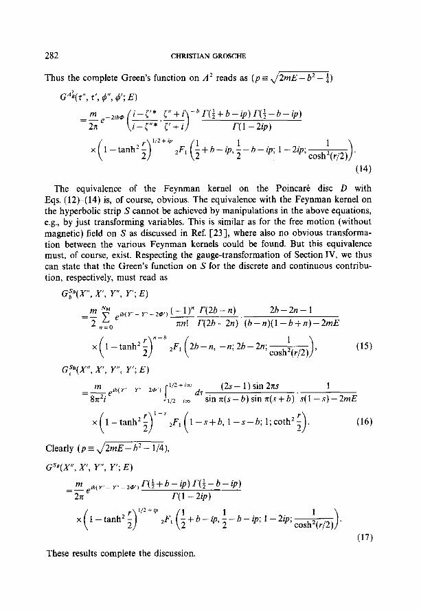
Thus the complete Green’s function on A2 reads as (p = ,/m)

Gni(Tft 9 r’, f’, 4’; E)

m -2ibQ i-c’* [“+i =iGe -.- ( i - err* [’ + i >

-bIJf+b-ip)T(i-b-ip) r(l-2ip)

(14)

The equivalence of the Feynman kernel on the Poincart disc D with Eqs. (12)-(14) is, of course, obvious. The equivalence with the Feynman kernel on the hyperbolic strip S cannot be achieved by manipulations in the above equations, e.g., by just transforming variables. This is similar as for the free motion (without magnetic) field on S as discussed in Ref. [23], where also no obvious transformation between the various Feynman kernels could be found. But this equivalence must, of course, exist. Respecting the gauge-transformation of Section IV, we thus can state that the Green’s function on S for the discrete and continuous contribu- tion, respectively, must read as

Gp(X”, X’, Y”, Y’; E)

=t F eib(y’-y”-2@‘) t-l)” r(2b-n) . 2b-2n- 1

?I=0 nn! r(2b-2n) (b-n){1 -b+n)-2mE

x(ltanh’fy-‘,f,(2b-n, -n;2b-2n;cosh~(r,2)), (15)

GF(X”, x’, Y”, Y’; E)

m eib(Y’- Y-228’)

s

l/2 + im

ds (2s - 1) sin 2ns 1

- 8z2i l/2-ice sinn(s-b)sinn(s+b)‘s(l-s)-2mE

x(l-tanh2~)1~‘2F,(l-sfb,l-s-b;l;coth2~). (16)

Clearly (p = 2/2mE- b2 - l/4),

GSB(X”, X’, Y”, Y’; E)

_ m eib( r’- Y” - 2125’) Q$+b-ip)r(;-b-ip) -27c r(l-2ip)

x(~-tanhz~)ln-c2f,(~+b-ip,f-b-~;~-2ip:cosh~(~,2)).

(17) These results complete the discussion.


ACKNOWLEDGMENT

I thank F. Steiner for reading the manuscript. It was a pleasure to talk with A. Inomata, J. I. Devreese, G. Junker, G. J. Papadopoulos, and L. Schulman at the Workshop on “Path Integrals and Quantum Chaos,” Hamburg, June S-6, 1989.

REFERENCES

1. A. M. ARTHURS, Proc. R. Sac. London A 313 (1969), 445. 2. R. AURICH, M. SIEBER, AND F. STEINER, Phys. Rev. L&t. 61 (1988), 483. 3. R. AURICH AND F. STEINER, Physica D 39 (1989), 69. 4. N. L. BALAZS AND A. VOROS, Phys. Rep. 143 (1986), 109. 5. A. 0. BARUT, A. INOMATA, AND G. JUNKER; J. Phys. A Math. Gen. 20 (1987), 6271. 6. A. 0. BARUT AND R. WILSON, Phys. Left. A 110 (1985), 351. 7. M. B~~HM AND G. JUNKER, Phys. Lett. A 117 (1986), 375. 8. M. B~HM AND G. JUNKER, J. Math. Phys. 28 (1987), 1978. 9. A. COMTAT, Ann. Phys. (N. Y.) 173 (1987), 185.

10. A. COMTET AND P. G. HOUSTON, J. M&h. Phys. 26 (1985), 185. 11. B. S. DEWITT, Reo. Mod. Phys. 29 (1957), 377. 12. 1. H. DURU, Phys. Rev. 030 (1984), 2121. 13. I. H. DURU AND H. KLEINERT, Phys. Left. B 84 (1979), 185; Fomchr. Phys. 30 (1982). 401. 14. J. FAY, J. Reine Angew. Math. 293 (1977), 143. 15. R. P. FEYNMAN, Rev. Mod. Phys. 20 (1948), 367. 16. A. FRANK AND K. B. WOLF, J. Math. Phys. 25 (1985), 973. 17. J. L. GERVAIS AND A. JEVICKI, Nucl. Phys. B 110 (1976), 93. 18. M. J. GOOVAERTS, J. Math. Phys. 16 (1975), 720. 19. I. S. GRADSHTEYN AND I. M. RYZHIK, “Table of Integrals, Series, and Products,” Academic Press,

San Diego, 1980. 20. M. B. GREEN, J. H. SCHWARZ. AND E. WITTEN, “Superstring Theory I, II,” Cambridge Univ. Press,

Cambridge, 1987. 21. C. GROSCHE, Phys. Left. A 128 (1988), 113. 22. C. GROSCHE, Ann. Phys. (N. Y.) 187 (1988), 110. 23. C. GROSCHE, Fortschr. Phys. 38 (19901, 71. 24. C. GROSCHE AND F. STEINER, Z. Phys. C 36 (1987), 699. 25. C. GROSCHE AND F. STEINER, Phys. Left. A 123 (1987), 319. 26. C. GROSCHE AND F. STEINER, Ann. Phys. (N. Y.) 182 (1988), 120. 27. C. GROSCHE AND F. STEINER, “Feynman Path Integrals,” in preparation. 28. M. C. GUTZWILLER, J. M&h. Phys. 8 (1967), 1979; Phys. Ser. T9 (1985), 184. 29. D. HEIHAL, “The Selberg Trace Formula for PSL(2, R),” Lecture Notes in Mathematics, Vol. 548,

Springer-Verlag, Berlin, 1976. 30. G. JUNKER AND A. INOMATA, “Bielefeld Encounters in Physics and Mathematics VII” (M. C.

Gutzwiller, A. Inomata, J. R. Klauder and L. Streit, Eds.), p. 315, World Scientific, Singapore, 1985. 31. R. KUBO, Prog. Theor. Phys. 78 (1987), 755; Prog. Theor. Phys. 79 (1988), 217. 32. T. D. LEE, “Particle Physics and Introduction to Field Theory,” Harwood Academic Press,

New York, 1981. 33. W. MAGNUS, F. OBERHETTINGER, AND R. P. SONI, “Formulas and Theorems for the Special

Functions of Theoretical Physics,” Springer-Verlag, Berlin, 1966. 34. M. S. MARINOV, Phys. Rep. 60 (1980), 1. 35. D. C. MCLAUGHLIN AND L. S. SCHULMAN, J. Math. Phvs. 12 (1971), 2520. 36. M. MIZRAHI, J. Math. Phys. 16 (1975), 2201.


37. M. OMOTE, Nucl. Phys. B 120 (1977), 325. 38. K. OSHIMA, Prog. Theor. Phys. 81 (1989), 286. 39. S. J. PATTERSON, Composiro Math. 31 (1975), 83. 40. D. PEAK AND A. INOMATA, J. Math. Phys. 10 (1969), 1422. 41. A. M. POLYAKOV, Phys. Left. B 103 (1981), 207. 42. G. P~SCHL AND E. TELLER, Z. Phys. 83 (1933), 143. 43. E. SCHR~~DINGER, Proc. R. Irish Sot. 46 (1941), 183. 44. L. S. SCHULMAN, “Technique and Applications of Path Integration,” Addison Wiley, New York,

1981. 45. A. SELBERG, J. Indian Math. Sot. 20 (1956), 47. 46. M. SIEBER AND F. STEINER, DESY preprints DESY 8943; DESY 89-093. 47. F. STEINER, “Bielefeld Encounters in Physics and Mathematics VII” (M. C. Gutzwiller, A. Inomata,

J. R. Klauder, and L. Streit, Eds.), p. 335, world Scientific, Singapore, 1985. 48. F. STEINER, “Recent Developments in Mathematical Physics,” Conference Schladming 1987

(H. Mitter and L. Pittner, Eds.), p. 305, Springer-Verlag, New York, 1987. 49. A. TERRAS, SIAM Rev. 24 (1982), 159; “Harmonic Analysis on Symmetric Spaces and Applications

I,” Springer-Verlag, New York, 1987. 50. H. A. VILENKIN, “Special Functions and the Theory of Group Representations,” Amer. Math. Sot.,

Providence, R. I., 1968.

path integration on the hyperbolic plane with a magnetic …€¦ · · 2007-03-09path...

Documents