path planning algorithms for robotic agentsmotion.me.ucsb.edu/pdf/phd-pa-jan16.pdf · path planning...
TRANSCRIPT

University of CaliforniaSanta Barbara
Path Planning Algorithms
for Robotic Agents
A dissertation submitted in partial satisfaction
of the requirements for the degree
Doctor of Philosophy
in
Mechanical Engineering
by
Pushkarini Agharkar
Committee in charge:
Professor Francesco Bullo, ChairProfessor Bassam BamiehProfessor Brad PadenProfessor Yasamin MostofiProfessor Joao Hespanha
March 2016
The Dissertation of Pushkarini Agharkar is approved.
Professor Bassam Bamieh
Professor Brad Paden
Professor Yasamin Mostofi
Professor Joao Hespanha
Professor Francesco Bullo, Committee Chair
June 2015

Path Planning Algorithms
for Robotic Agents
Copyright c� 2016
by
Pushkarini Agharkar
iii

To my father,
Dr. Hemchandra Agharkar (M.D, D.P.M)
iv

Acknowledgements
First and foremost, I would like to thank my advisor Professor Francesco Bullo for
advising me in my research at UCSB. I thank him for being a great role model, for his
immense patience and for teaching me the best research practices. I would also like to
thank him for encouraging the wonderful environment of the motion lab. I would also
like to thank Dr. Shaunak Bopardikar for mentoring me through the thought process
which resulted in what is the second chapter of this thesis. I would also like to thank
Rushabh Patel for a collaboration which led to results in the third chapter of this thesis,
as well as my other collaborators Dr. Sara Susca and Prof. Sonia Martinez. I thank my
dissertation committee for providing their time and advice.
I would like to thank Prof. Niket Kaisare and Prof. R. I. Sujith from IIT Madras.
Its due to their encouragement and guidance that I deciced to pursue these four years
of research. I would like to thank friends from the motion lab especially Anahita, Fabio,
Vaibhav, Je↵, Wenjun and Sepehr for their gestures big and small. I would like to thank
Prof. Scott Marcus for his inspiring attitude, his sitar lessons and also our sitar ensemble
at UCSB.
I am grateful to have supportive roommates like Stephanie, Christine and Amber
throughout these years. I thank them for introducing me to this country. I am thankful
to Mani, Bonnie, Raga and Vikram for wonderful vacations and time-outs. I am terribly
lucky to have friends like Santosh, Dinesh and Sumit in Santa Barbara. The time spent
with them and our bond has kept me afloat and given me so much to look forward to. I
would also like to thank Sushant for helping me transition out of graduate school.
I thank Ramani for growing up when I wasn’t looking and for advising and encour-
aging me in work and other matters. I thank my mother for passing on the joie de
vivre.
v

Curriculum VitæPushkarini Agharkar
Education
2011 B.Tech. in Aerospace Engineering, Indian Institute of TechnologyMadras.
2011 M.Tech. in Aerospace Engineering, Indian Institute of TechnologyMadras.
Work Experience
Jul-Sept 2014 Summer Intern, Bosch LLC, Palo Alto, California
May-Jul 2010 Research Intern, Ecole Polytechnique, Paris, France
May-Jul 2009 Summer Intern, Larsen & Toubro, Mumbai, India
Selected Publications
(J1) Vehicle Routing Algorithms for Radially Escaping Targets. P. Agharkar, S. D.Bopardikar, F. Bullo, SIAM Journal on Control and Optimization, Note: submitted.
(J2) Quickest Detection over Robotic Roadmaps. P. Agharkar, F. Bullo, IEEE Transac-tions on Robotics, Note: submitted.
(J3) Robotic Surveillance and Markov Chains with Minimal First Passage Time. R.Patel, P. Agharkar, F. Bullo, IEEE Transactions on Automatic Control, Note: ac-cepted.
(J4) Synchronization of Beads on a Ring by Feedback Control. S. Susca, P. Agharkar,S. Martinez, F. Bullo, SIAM Journal on Control and Optimization, 52(2): 914-938,2014.
(C1) Robotic Surveillance and Markov Chains with Minimal First Passage Time. P.Agharkar, P. Patel, F. Bullo, IEEE Conf. on Decision and Control, Los Angeles,CA, USA, pages 6603-6608, Dec. 2014.
(C2) Vehicle Routing Algorithms to Intercept Escaping Targets. P. Agharkar, F. Bullo,American Control Conference, Portland, OR, USA, pages 952-957, June 2014
vi

Abstract
Path Planning Algorithms
for Robotic Agents
by
Pushkarini Agharkar
The focus of this work is path planning algorithms for autonomous agents. Specifically,
we study problems in three areas where path planning to direct the motion of autonomous
agents is critical for their performance. The first problem is a vehicle routing problem in
which mobile demands appear in an environment and the task of the autonomous agent
is to stop the demands from escaping the environment boundary. We first propose two
fundamental performance bounds for the proposed problem. We then propose routing
algorithms for this problem with performance guarantees. We examine the gap between
these guarantees and the fundamental performance bounds. The second problem is a
surveillance problem in a networked environment. The tasks of the autonomous surveil-
lance agent in this problem are to (1) detect unknown intruder locations and (2) detect
anomalies based on noisy measurements. We propose Markov chain based routing algo-
rithms for the surveillance agent to achieve these goals. We parameterize these routing
algorithms using a property of Markov chains called the mean first passage time. We
also frame optimization problems to obtain optimal algorithms for the two surveillance
tasks. The third problem studied in this work is a boundary guarding problem in which
the task of a set of patrolling agents constrained to move on a ring is to achieve syn-
chronization using only local communication. We propose a coordination algorithm to
solve this problem and identify initial agent configurations under which synchronization
is guaranteed.
vii

Contents
Curriculum Vitae vi
Abstract vii
List of Figures x
List of Tables xiii
1 Introduction 11.1 Vehicle Routing Problems . . . . . . . . . . . . . . . . . . . . . . . . . . 21.2 Robotic Surveillance . . . . . . . . . . . . . . . . . . . . . . . . . . . . . 51.3 Boundary Guarding and Coordination . . . . . . . . . . . . . . . . . . . 81.4 Organization . . . . . . . . . . . . . . . . . . . . . . . . . . . . . . . . . 9
2 Radially Escaping Targets Problem 112.1 Contributions . . . . . . . . . . . . . . . . . . . . . . . . . . . . . . . . . 122.2 Organization . . . . . . . . . . . . . . . . . . . . . . . . . . . . . . . . . 142.3 Problem Formulation . . . . . . . . . . . . . . . . . . . . . . . . . . . . . 142.4 Preliminary results . . . . . . . . . . . . . . . . . . . . . . . . . . . . . . 152.5 Policies . . . . . . . . . . . . . . . . . . . . . . . . . . . . . . . . . . . . . 272.6 Simulations . . . . . . . . . . . . . . . . . . . . . . . . . . . . . . . . . . 33
3 Robotic Surveillance: Detection of Intruder Location 433.1 Contributions . . . . . . . . . . . . . . . . . . . . . . . . . . . . . . . . . 443.2 Organization . . . . . . . . . . . . . . . . . . . . . . . . . . . . . . . . . 443.3 The Kemeny constant and its minimization . . . . . . . . . . . . . . . . . 463.4 The weighted Kemeny constant and its minimization . . . . . . . . . . . 533.5 Applications of the mean first passage time to surveillance . . . . . . . . 63
4 Robotic Surveillance: Quickest Anomaly Detection 754.1 Contributions . . . . . . . . . . . . . . . . . . . . . . . . . . . . . . . . . 764.2 Organization . . . . . . . . . . . . . . . . . . . . . . . . . . . . . . . . . 76
viii

4.3 Problem Setup . . . . . . . . . . . . . . . . . . . . . . . . . . . . . . . . 774.4 Preliminary Results . . . . . . . . . . . . . . . . . . . . . . . . . . . . . . 804.5 Performance of the Ensemble CUSUM Algorithm . . . . . . . . . . . . . 824.6 Numerical Simulations . . . . . . . . . . . . . . . . . . . . . . . . . . . . 89
5 Synchronization of Beads on a Ring 945.1 Contributions . . . . . . . . . . . . . . . . . . . . . . . . . . . . . . . . . 955.2 Organization . . . . . . . . . . . . . . . . . . . . . . . . . . . . . . . . . 955.3 Model and problem statement . . . . . . . . . . . . . . . . . . . . . . . . 965.4 Synchronization algorithm . . . . . . . . . . . . . . . . . . . . . . . . . . 985.5 Preliminary results . . . . . . . . . . . . . . . . . . . . . . . . . . . . . . 1025.6 Convergence analysis . . . . . . . . . . . . . . . . . . . . . . . . . . . . . 1055.7 Simulations . . . . . . . . . . . . . . . . . . . . . . . . . . . . . . . . . . 113
6 Conclusions and Future Directions 1346.1 Radially Escaping Targets Problem . . . . . . . . . . . . . . . . . . . . . 1346.2 Quickest Detection of Intruder Location . . . . . . . . . . . . . . . . . . 1356.3 Quickest Detection of Anomalies . . . . . . . . . . . . . . . . . . . . . . . 1366.4 Synchronization of beads on a ring . . . . . . . . . . . . . . . . . . . . . 137
Bibliography 139
ix
List of Figures
2.1 (a) Schematic of the Radially escaping targets (RET) problem. (b) Theparameter regimes where the Stay-at-Center (SAC), Sector-Wise(SW) andStay-Near-Boundary(SNB) policies are designed are shown for D=1. Thegray shaded regions indicate the parameter regimes in which the policiesare constant factor optimal. . . . . . . . . . . . . . . . . . . . . . . . . . 12
2.2 Optimal vehicle location x⇤ and the maximum probability ⇢⇤ of capturingan escaping target starting from (x⇤, 0) as a function of target speed v forthe RET problem with D = 1. . . . . . . . . . . . . . . . . . . . . . . . . 19
2.3 (a) The set ST for the RET problem is shown by the gray shaded region.The dashed circle is the boundary of ST which is a circle of radius Tcentered at (X � vT, 0). (b) The area element ⇣ of length and width m inST . . . . . . . . . . . . . . . . . . . . . . . . . . . . . . . . . . . . . . . . 22
2.4 The thick line labeled Ti+1
indicates the trajectory of the vehicle startingfrom the target i to service the target i+ 1. The gray circles indicate thelocations at which the vehicle intercepts the targets. . . . . . . . . . . . . 26
2.5 (a) Vehicle located at p = (X, 0) services outstanding targets shown bythe shaded region. (b) Factor of optimality of the SW policy in di↵erentparameter regimes v,� when D = 1. . . . . . . . . . . . . . . . . . . . . . 29
2.6 Performance of the (a) SAC and (b) SW policies for arrival rates � = 2and � = 10 respectively for the RET problem with D = 1. The theoreticalbounds are from Theorem 12 and Theorem 15 respectively. . . . . . . . . 34
3.1 Example of a doubly-weighted graph G = (V , E, P,D) with three nodes:(a) shows the edge set, E, allowed for the graph with three nodes, (b)shows the probabilities, pij to move along each edge, and (c) shows thetime (i.e., distance traveled), dij to move along each edge. . . . . . . . . . 54
3.2 Environment with two obstacle represented by an unweighted graph. . . 663.3 Various airport hub locations (top), and the corresponding weight map
(bottom). Edge weights between two hubs account for travel time betweenhubs plus required service time once at hub. Self loops have no travel timeso encompass only service time required at hub. . . . . . . . . . . . . . . 67
x
3.4 Percentage of intruders detected for varying intruder life-times by a surveil-lance agent executing a random walk according to the Markov chain gen-erated by the mean first-passage time algorithm (circle), FMMC algorithm(square), M-H algorithm (asterisk), and the Markov chain generated bysolving Problem 5 (diamond). Average points and standard deviation er-ror bars are taken over 200 runs, where the intruder appears 500 times foreach run. . . . . . . . . . . . . . . . . . . . . . . . . . . . . . . . . . . . . 68
4.1 The environment is an area separated into seven regions of interest. Ob-servations made in the highlighted region change after an anomaly occurs.The aim of the surveillance vehicle is to detect this change as soon aspossible. . . . . . . . . . . . . . . . . . . . . . . . . . . . . . . . . . . . . 78
4.2 The robotic roadmap corresponding to the environment can be representedby a graph. The edge weights of the graph represent travel times betweenneighboring regions. . . . . . . . . . . . . . . . . . . . . . . . . . . . . . . 78
4.3 Variation of the average detection delay using the optimal policy �⇤avg
(blacksquares), the e�cient policy �
ub
(grey squares), the policy based on thefastest mixing non-reversible Markov chain with a uniform stationary dis-tribution (grey circles) and the policy in [95] (black circles) with respectto the threshold ⌘ of the CUSUM algorithm. Expected detection delay forthe optimal policy using Monte Carlo Simulations (dashed lines). . . . . 90
4.4 Average detection delay using the optimal policy �⇤avg
(black squares) andthe e�cient policy �
ub
(grey squares) are compared with the average de-tection delay obtained using the policy based on the fastest mixing non-reversible Markov chain (grey circles) with a uniform stationary distribu-tion and the policy from [95] (black circles) for various levels on noise inobservations made in the second region. . . . . . . . . . . . . . . . . . . . 90
5.1 The figure shows a collection of four beads moving in balanced synchro-nization. . . . . . . . . . . . . . . . . . . . . . . . . . . . . . . . . . . . . 97
5.2 This figure shows that, regardless from where and with which velocitiesbeads i and i+1 impact, the order of the beads is preserved. The velocitiesin the figure are the velocities after the impact. The speed v is just theaverage value of vi and vi+1
before the impact. . . . . . . . . . . . . . . . 1045.3 This figure shows the periodic orbit described in Theorem 50. The white
circles are the positions of beads. The black dots are the locations of theimpacts for any two neighboring beads. Note that bead i� 1 and i� 2 aremoving towards each other and so are beads i and i+ 1. . . . . . . . . . 110
5.4 This figure illustrates G(t) for t 2 [I1,2, I1,2 + 22⇡
n1
v] and the time at which
each edge appears for n = 5 andPn
i=1
di(0) = �1 when unbalanced syn-chrony is reached. . . . . . . . . . . . . . . . . . . . . . . . . . . . . . . . 111
xi
5.5 The SIS Algorithm is implemented with n = 8 beads, which are ran-domly positioned on S1, vi(0) is uniformly distributed in ]0, 1], d
1
(0) =d2
(0) = d4
(0) = d6
(0) = +1, and f = 0.7. (a) shows positions of beadsvs time. Beads 2, 4, 6, 8 are represented by solid lines, while the dash line,dash-dot line, point line, and thicker dash line represent the positions ofbeads 1, 3, 5, 7. (b) shows ✓
5
(t) (solid line), u5
(t) (thicker solid line), and`5
(t) (dash-dot line). . . . . . . . . . . . . . . . . . . . . . . . . . . . . . 1155.6 The SIS Algorithm is implemented for n = 7 beads. The beads are
randomly positioned on S1, vi(0) is uniformly distributed in ]0, 1], d1
(0) =d4
(0) = d5
(0) = d7
(0) = �1, and f = 0.6. (a) shows ✓i vs time. Beads2, 4, 6 are represented by solid lines, while the dash line, dash-dot line,point line, and thicker dash line represent the positions of beads 1, 3, 5, 7.(b) shows ✓
3
(t) (solid line), u3
(t) (thicker solid line), and `3
(t) (dash-dotline). . . . . . . . . . . . . . . . . . . . . . . . . . . . . . . . . . . . . . . 116
5.7 The SIS Algorithm is implemented for n = 12 beads. The beads arerandomly positioned on S1, vi(0) is uniformly distributed in ]0, 1], d
1
(0) =d2
(0) = d4
(0) = d6
(0) = d7
(0) = d9
(0) = d12
(0) = �1, and f = 0.84. (a)shows positions of the beads vs time. Beads 2, 4, 6, 8, 10, 12 are representedby solid lines, while the dash line, dash-dot line, point line, and thickerdash line represent the positions of beads 1, 3, 5, 7, 9, 11. (b) shows ✓
3
(t)(solid line), u
3
(t) (thicker solid line), and `3
(t) (dash-dot line). . . . . . . 1175.8 This figure shows ✓i vs time, obtained by implementing the SIS Algo-
rithm with n = 12 beads, the beads are randomly positioned on S1,vi(0) uniformly distributed in ]0, 1], d
1
(0) = d4
(0) = d6
(0) = d7
(0) =d8
(0) = d9
(0) = d10
(0) = �1, and f = 0.87. The positions of the beads2, 4, 6, 8, 10, 12 are represented by solid lines, while the dash line, dash-dot line, point line, and thicker dash line represent the positions of beads1, 3, 5, 7, 9, 11. . . . . . . . . . . . . . . . . . . . . . . . . . . . . . . . . . 118
5.9 This figure shows how the speeds of bead i and i + 1 change while theyare traveling towards each other. Note that bead i is early with respect tobead i+ 1. . . . . . . . . . . . . . . . . . . . . . . . . . . . . . . . . . . . 121
5.10 From top to bottom, the figure illustrates the position of Ci�1
, Ci, and ofui�1
� � �� for � < ⇡nand � > ⇡
n. . . . . . . . . . . . . . . . . . . . . . 124
5.11 This figure shows how the speeds of bead 1 and 2 change as they aretraveling towards each other, shortly after bead 1 meets bead n. . . . . . 131
xii

List of Tables
2.1 Performance of policies for the RET problem . . . . . . . . . . . . . . . . 13
3.1 Statistics on the percentage of intruders caught in 200 simulation runs forthe environment in Fig. 3.2. . . . . . . . . . . . . . . . . . . . . . . . . . 66
3.2 Statistics on the percentage of intruders caught in 200 simulation runs forthe environment in Fig. 3.3. . . . . . . . . . . . . . . . . . . . . . . . . . 68
xiii
Chapter 1
Introduction
Autonomous robotic agents have numerous applications, for instance in hospital and
o�ce delivery system [89],[56], as museum tour guides [23], for topological mapping [99],
in warehouse management [106] and building maintenance and surveillance [68]. Apart
from the onboard sensors and the dexterity of the robots, the performance of these robots
depends on the path planning algorithms, that is, the algorithms which determine their
motion in the environment under service. In order to optimize the performance of the
robots, these algorithms have to deal with various service allocation problems as well as
facilitate coordination amongst robots in a multi-robot system.
We focus our attention of the motion planning of autonomous robots in three specific
areas- (1) vehicle routing problems, (2) surveillance for intruder and anomaly detection
and (3) coordinated boundary guarding. We now review the current literature in these
areas. We will also state the motivation for the problem setups considered in the next
chapters.
1

Introduction Chapter 1
1.1 Vehicle Routing Problems
The Vehicle Routing Problem (VRP) was first introduced by [31] and has received
wide attention for a long time [62],[43]. Due to a recent surge of activity in the area of
motion planning for autonomous robots, a lot of variants of the VRP have been addressed
over the last decade. An extensive list of such problems can be found in [22].
The most well-known VRP is arguably the classical Traveling Salesman Problem
(TSP). In the TSP, a traveling salesman has to conduct the shortest tour of a given
number of cities, visiting each city exactly once. The TSP like most other VRPs is NP-
hard. The TSP and its extensions to other VRP problems have been explored extensively
[11, 100]. Of the numerous extensions of the VRP, these are the extensions particularly
relevant to the specific problem that we study:
(1) Dynamic Vehicle Routing (DVR) [83] problems, in which the arrival process of the
demands to be serviced is stochastic.
(2) VRP with time-windows [33],[100], in which demands have to be serviced within a
time-window.
(3) VRP with moving demands [48] where the vehicle has to intercept demands moving
with arbitrary velocities.
The problem introduced in Chapter 2 draws from all these extensions. We now review
some problems and the algorithms proposed for them in these extension areas, with
particular attention to the VRP with moving targets, and also justify our problem setup.
(Dynamic Vehicle Routing): In DVR problems, demands arrive according to a
stochastic rather than a deterministic process. This setup is motivated by stochastic
arrival of demands in di↵erent applications, e.g. demands for services [98, 10] or goods
[42, 7]. In DVR problems at least a part of the input is unknown to the vehicle and the
2
Introduction Chapter 1
vehicle has to modify its path based on real-time information of new demand locations. In
contrast to static vehicle routing, these problems hence require routing policies instead
of pre-planned routes. The dynamically changing routes which are a result of these
routing policies can be computed and executed due to technological advances like the
introduction of the GPS and GIS and the widespread use of mobile and smartphones.
A review of Dynamic Vehicle Routing Problems was conducted in [83]. An example
DVR problem which is also arguably the most general model for vehicle routing problems
that have both a dynamic and a stochastic component is the m�vehicle Dynamic Trav-
eling Repairman Problem (m-DTRP), which was introduced by [84] and mainly studied
by Bertsimas and van Ryzin in [11], [12] and [13]. In [80] authors introduce policies for
the m-DTRP which are adaptive with respect to the environment parameters and also
provably optimal in light and heavy demand load conditions.
(VRP with time-windows): In situations where the demands are active only for a
limited time period, time-windows are introduced in the setup of the VRP. This modi-
fication can enhance customer satisfaction and is necessary in situations where demand
generation degrades over time, e.g. in the case of sensors which are active for some time
on receiving information before going into an energy-saving “sleep” mode. The VRP
with time-windows (VRPTW) was reviewed in [63]. Significant progress has been made
in this class of VRPs, see for example, [93, 100, 20, 34]. In [79], authors model the prob-
lem with time-windows in a dynamic environment. They also consider stochastic time
windows within which targets are required to be serviced. Modified versions of VRP with
time-windows have been studied in [15, 79].
(VRP with moving demands): Several researchers have worked on dynamic vehi-
cle routing problems (VRPs) involving moving targets in the past. The approximation
complexity of Moving-Target TSP was studied in [46], where it was shown that Moving-
Target TSP with n targets cannot be approximated better than by a factor of 2O(
pn)
3
Introduction Chapter 1
times optimal within polynomial time unless P = NP . The authors in the same work
also showed that if targets have the same velocities, then there is a polynomial time
approximation for the Moving-Target TSP. Authors in [48] give a 2 + ✏ approximation
algorithm for instances of the Moving-Target TSP in which O( lognlog logn
) of the n points
are moving with arbitrary velocity. Authors in [16] study a variant of the Moving-Target
VRP in which targets appear on a segment and move with the same velocity. They prove
that a first come first serve policy minimizes the expected time to service a target when
the target arrival rate is very high as well as when the target speed is close to the vehicle
speed. Authors in [26] study a kinetic variant of the k-delivery TSP where all targets
move with the same velocity and a robotic arm moving with a finite capacity must in-
tercept them. They provide constant-factor approximation for the problem. Authors
in [6] study a grasp and delivery problem motivated by robot navigation and propose a
2-factor approximation algorithm. In [15], the moving targets have to be serviced within
a time-window and a policy based on repeated computation of longest paths through the
available set of targets is proposed to this end.
Apart from the above broader areas, more recent results on the subject of routing
problems involving the task of target interception consider more general models for target
behavior [8, 66, 61]. In [8], the authors propose a partitioning strategy for a multiple
vehicle multiple target problem in which the targets can apply an evading strategy in
response to the actions of the service vehicle. We consider a vehicle routing problem in
which demands appear according to a stochastic process. On appearing, they move in
the radially outward direction so that all demands have di↵erent speeds, depending on
where they originate in the environment. The time-windows within which they need to
be serviced also depend on their point of origin. They do not, however, modify their
direction to evade an approaching vehicle.
Motivation: The problem setup in Chapter 2 is significantly di↵erent from earlier
4

Introduction Chapter 1
setups in the following ways: The moving targets have di↵erent velocities depending on
their angular location, as opposed to having same velocities as assumed in many problem
setups looked at in literature [16, 46, 90, 79]. They also have di↵erent deadlines depending
on their radial location as opposed to having the same deadline or time window before
which they should be serviced [15, 16]. They move along radial direction so as to escape
the environment as quickly as they can. One application of this problem setup is in
robotic patrolling where it is necessary to stop malicious agents from leaving a region so
as to protect the surroundings.
1.2 Robotic Surveillance
The second area of application which we study is robotic surveillance. The surveil-
lance problem has appeared in the literature in various manifestations. Theoretical anal-
ysis of the surveillance problem was conducted in [28] and a survey of various surveillance
scenarios and the corresponding approaches was presented in [4]. Surveillance strategies
that minimize the refresh time, i.e. time period between subsequent visits to regions
have been proposed in [76],[91] and [92]. In [76], authors propose optimal algorithms
which minimize the refresh time for chain and tree graphs and constant factor algorithm
for cyclic graphs. Authors in [92] consider the problem of minimizing specific weighted
sums of refresh times and design non-intersecting tours on graphs for this surveillance
criterion. In [91], the authors design speed controllers on closed paths to minimize the
refresh time for a given set of points of interest in the environment.
The surveillance policies proposed in [76],[91] and [92] are deterministic in nature.
Stochastic surveillance strategies assume importance in scenarios where the intruders can
move or hide to avoid detection and as a result, the movement of the surveillance vehicle
is required to be non-deterministic. A main result of [94] also shows that deterministic
5
Introduction Chapter 1
policies are ill-suited when designing strategies with arbitrary constraints on those visit
frequencies. Several authors have used Markov chain based approaches to design stochas-
tic strategies for various surveillance tasks. Authors in [94] use the Metropolis-Hastings
algorithm to achieve specified frequency of visits to regions of the environment. In [44],
authors design random walk strategies on hypergraphs and parametrically vary the local
transition probabilities over time in order to achieve fast convergence to a desired visit
frequency distribution. In [95], authors use the fastest mixing Markov chain for quickest
detection of anomalies.
Motivated by practical applications, the surveillance problem has also been dealt with
in other innovative ways. For example authors in [87] consider di↵erent intruder models
and present routing strategies for surveillance in scenarios corresponding to them. In [67]
wireless sensor networks are utilized for intruder detection in previously unknown environ-
ments. In [5], the authors explore strategies for surveillance using a multi-agent ground
vehicle system which must maintain connectivity between agents. A non-cooperative
game framework is utilized in [27] to determine an optimal strategy for intruder detec-
tion, and in [77] a similar framework is used to analyze intruder detection for ad-hoc
mobile networks.
We consider two problems within the broad area of robotic surveillance, the first one
is concerned with the detection of unknown intruder location and the second with the
quickest detection of anomalies in networked environments. We propose Markov chain
based routing strategies for the problems. Both the problems and the proposed robotic
routing strategies are parameterized by the metric called the mean first passage time of
Markov chains. We now present the literature on the mean first passage time.
For a random walk associated with a Markov chain, the mean first passage time, also
known as the Kemeny constant, of the chain is the expected time taken by a random
walker to travel from an arbitrary start node to a second randomly-selected node in a
6

Introduction Chapter 1
network. The Kemeny constant of a Markov chain first appeared in [55] and has since
been studied by several scientists, e.g., see [52, 58] and references therein. Bounds on the
mean first passage time for an arbitrary Markov chain over various network topologies
appear in [52, 64].
The mean first passage time is closely related to other well-known metrics for graphs
and Markov chains. We discuss two such quantities in what follows. First, the Kirchho↵
index [59], also known as the e↵ective graph resistance [38], is a related metric quan-
tifying the distance between pairs of vertices in an electric network. The relationship
between electrical networks and random walks on graphs is explained elaborately in [37].
For an arbitrary graph, the Kircho↵ index and the Kemeny constant can be calculated
from the eigenvalues of the conductance matrix and the transition matrix, respectively.
The relationship between these two quantities for regular graphs is established in [75].
Second, the mixing rate of an irreducible Markov chain is the rate at which an arbitrary
distribution converges to the chain’s stationary distribution [35]. It is well-know that
the mixing rate is related to the second largest eigenvalue of the transition matrix of the
Markov chain. The influential text [65] provides a detailed review of the mixing rate and
of other notions of mixing. Recently, [58] refers to the Kemeny constant as the “expected
time to mixing” and relates it to the mixing rate.
Motivation: There are several motivations for the problem setups considered in
Chapter 3 and 4. First of all, the setups highlight the e↵ectiveness of the notion of the
mean first passage time which is relevant to surveillance tasks in which each region should
be accessible from the other regions in the environment in minumum time. The setups
also take into account travel times required by robotic agents to travel across the regions
of a networked environment. Third, the mean first passage time, which we analyze in
the process of proposing strategies for the two problems is of independent mathematical
interest and has applications potentially outside the area of robotics, e.g. in determining
7
Introduction Chapter 1
how quickly information propagates in an online network [9] or how quickly an epidemic
spreads through a contact network [105]. Lastly, the problem setups are motivated by
realistic surveillance scenarios, namely detection of an unknown intruder location in least
amount of time (Chapter 3) and surveillance under extreme modelling uncertainty and
measurement noise (Chapter 4).
1.3 Boundary Guarding and Coordination
The third area of application is the problem of guarding environment boundaries.
We study a multi-agent boundary guarding problem in which the agents achieve syn-
chronization in motion along the boundary of the environment. The synchronization
problem can also be seen as a consensus problem in which the agents reach consensus on
the environment partition in order to service the environment in a distributed manner.
Consensus algorithms have been extensively studied, beginning with the early work
on averaging opinions and stochastic matrices in [32]. For the setting of non-degenerate
stochastic matrices, [102] gives convergence conditions for consensus algorithms under
mild connectivity assumptions. Recent references on average consensus, algebraic graph
methods and symmetric stochastic matrices include [72, 54]. Recent surveys [40, 74, 85]
discuss attractive properties of these algorithms such as convergence under delays and
communication failures, and robustness to communication noise.
Synchronization in itself has been a widely studied problem and has been explored
for multi-agent system coordination; e.g. see [104, 36, 73, 70, 82]. In [104] a general-
ized distributed network of nonlinear dynamic systems with access to global information
is considered and synchronization in the network is shown to occur for strong enough
coupling strengths. The authors in [36] and [73] present distributed algorithms using
which synchronization is achieved in multi-agent systems using event triggered and self
8

Introduction Chapter 1
triggered control respectively. The authors in [70] draw analogies between impulsive and
di↵usive synchronization in the weak coupling limit.
References on the problem of perimeter estimation and monitoring by mobile robots
include [29, 107, 97, 101]. Patrolling problems have also been studied in [76, 2, 69]. More
relevant to the problem setup in this chapter are the studies in [25, 57], which make
use of the steady-state orbit for even number of synchronized agents described here and
referred to as ‘balanced’ synchronization.
Motivation: A possible worldly motivation for the study of this class of algorithms
is the surveillance of regions in a 2D space. Some examples of similar problems in
literature include [25, 57]. In [25] pairs of agents have to be released at particular points,
sequentially, and with the same speed. In contrast, in our algorithm the number of agents
can be odd, the agents can be released at arbitrary positions and with arbitrary speeds.
The distributed algorithm in [57] requires only that the agents move with a fixed speed.
However, it can not be easily extended to a perimeter which is a closed curve unless the
agents are assumed to have unique identifiers. Further, we stabilize a broader range of
trajectories, namely ‘unbalanced’ synchronization.
Apart from the application in boundary-patrolling, the study of the n beads problem
can find justification on more fundamental grounds. Namely, the investigation of under
what conditions systems subject to impacts and controlled dynamics are robustly stable,
and what techniques can be useful helpful in proving such stability properties. Both
these aspects have motivated us to consider this synchronization problem.
1.4 Organization
The thesis is organized as follows. In Chapter 2, we introduce and analyze the Radially
Escaping Targets problem and propose routing policies for autonomous agents for this
9
Introduction Chapter 1
problem. In Chapter 3 and Chapter 4 we study two surveillance problems. We propose
routing policies for surveillance agents in the two setups, employing the notion of the
mean first passage times of Markov chains in both the cases. In Chapter 5 we study a
boundary patrolling problem involving consensus between robotic agents using limited
communication. Finally, in Chapter 6 we summarize the results of the previous chapters
and also list some open problems.
10

Chapter 2
Radially Escaping Targets Problem
The various extensions of the vehicle routing problems were discussed in Section 1.1. In
this chapter we propose a novel vehicle routing problem involving moving targets. In
the setup of this problem, a single target maintains the same velocity throughout with
the intention of escaping the environment as quickly as possible. One application of this
problem setup is in robotic patrolling where it is necessary to stop malicious agents from
leaving a region so as to protect the surroundings.
The problem setup in this chapter is significantly di↵erent from earlier setups in the
following ways: The moving targets have di↵erent velocities depending on their angular
location, as opposed to having same velocities as assumed in many problem setups looked
at in literature [16, 46, 90, 79]. They also have di↵erent deadlines depending on their
radial location as opposed to having the same deadline or time window before which they
should be serviced [15, 16].
11

Radially Escaping Targets Problem Chapter 2
2.1 Contributions
The contributions of this chapter 1 can be summarized as follows. We introduce
a novel dynamic vehicle routing problem termed the Radially Escaping Targets (RET)
problem. The RET problem has three parameters: the target arrival rate �, the target
speed v < 1 and the environment radius D.
Stay-at-Center
Sector-Wise
0 0.2 0.4 0.6 0.8 10
10
20
30
40
50
target speed, v
arriv
al ra
te,λ
Stay-Near-Boundary(a) (b)
D(0,0)
rθ
v
Figure 2.1: (a) Schematic of the Radially escaping targets (RET) problem. (b) Theparameter regimes where the Stay-at-Center (SAC), Sector-Wise(SW) and Stay-N-ear-Boundary(SNB) policies are designed are shown for D=1. The gray shaded regionsindicate the parameter regimes in which the policies are constant factor optimal.
We first determine two policy independent upper bounds on the fraction of targets
that can be captured for the RET problem. In the process, we derive a novel method to
establish upper and lower bounds on the path through radially escaping targets. Next,
we formulate three policies: Stay-at-Center (SAC), Sector-wise (SW) and Stay-Near-
Boundary (SNB) policy. The SAC policy is designed for low arrival rates while the SW
policy is formulated for moderate arrival rates. The SNB policy is designed for high
arrival rates. Lower bounds on the fraction of targets captured using the SAC, SW and
SNB policies are obtained. In Table 2.1, we summarize these lower bounds and also
present the factor of optimality (defined as the ratio of the fundamental upper bound for
1This work is a product of collaboration with Dr. Shaunak Bopardikar
12

Radially Escaping Targets Problem Chapter 2
the RET problem to the capture fraction of a policy). The symbol � ⇡ 0.7120± 0.0002
and
↵(v) =
pv
⇡2
✓
v
(1� v2)3/2
◆
1/2
+10
3
(1� v2)1/2
v
!�1/2
.
In Fig. 2.1(b), the design regimes for the SAC, SW and SNB policies are shown. The
gray shaded regions indicate the regimes where the policies are constant factor optimal.
The SAC and SNB policy are constant factor optimal in the asymptotic regimes of
� ! 0+ and � ! +1 respectively. The gray shaded regions separated by dashed lines
are representative of these asymptotic regimes. For fixed target speed, the SW policy
is within a constant factor of the optimal in the gray shaded region in the middle. We
present numerical simulations which empirically verify our results.
Table 2.1: Performance of policies for the RET problem
Design Regime Algorithm Regime of Factor
constant factor optimality of optimality
Light load Stay-At-Center �! 0+ 1
Moderate load Sector-wise � >7⇡v
(1� v2)3/2D, v >
1
4p2
1
↵(v)
Fixed speed, heavy load Stay-Near-Boundary �! +1, D > 17�
2
The set-up of the RET problem can be viewed as a dynamical system where targets
are generated via a stochastic process. The dynamical system needs to be controlled
using a control law or policy in order to stop the targets from escaping the environment.
The performance metric to evaluate the policy is the capture fraction of the targets which
needs to be maximized. Fundamental upper bounds and achievable lower bounds on the
capture fraction is the topic of the chapter. We study the gap between them as well.
13

Radially Escaping Targets Problem Chapter 2
2.2 Organization
This Chapter is organized as follows. In Section 2.1 we state the contributions of the
work. In chapter 2.3 we describe the problem setup. The preliminary results are stated
in Section 2.4 and the main results, i.e. the routing policies for the proposed problem are
presented in 2.5. The chapter ends with numerical simulations presented in Section 2.6.
2.3 Problem Formulation
We start with introducing a DVR problem in which the environment is a disk of
radius D given by:
E = {(r, ✓) : 0 r D 8✓ 2 [0, 2⇡)} .
Targets appear independently and uniformly distributed in E with uniform spatial den-
sity. Their arrival times are modeled using a Poisson process with rate � [86]. Uni-
form spatial distribution of the targets is realized through probability density functions
f(r) = 2r/D2 and e(✓) = 1/2⇡ where r and ✓ are random variables describing the lo-
cation of appearing targets in radial coordinates. Once the targets appear, they move
radially outwards with a constant speed v < 1 and eventually reach the boundary of
the environment. A vehicle with speed of 1 and confined to move in E intercepts the
targets and captures them before they escape the environment. We refer to this problem
as the Radially Escaping Targets (RET) problem for convenience and a schematic of the
problem is shown in Fig. 2.1(a). The parameters of the RET problem are the target
speed v, arrival rate � and disk radius D.
Let Q(t) ⇢ E denote the set of positions of all targets that have appeared but have
not been serviced or have escaped before time t. Let p(t) 2 E be the position of the
vehicle at time t. A policy for the vehicle is a map P : E ⇥ FIN(E)! R2, where FIN(E)
14

Radially Escaping Targets Problem Chapter 2
is the set of finite subsets of E , assigning a velocity to the service vehicle as a function
of the current state of the system: p(t) = P (p(t),Q(t)). Let mcap
(t) be the number of
targets that have appeared and have been captured before time t and mmiss
(t) be the
number of targets that have escaped and mtot
(t) = mmiss
(t) +mcap
(t), then the goal of
this problem can be stated as follows:
Problem Statement Find policies P that maximize the fraction of targets that are
serviced Fcap
(P ), termed as the capture fraction. Formally, for a policy P , we define the
steady state average capture fraction as
Fcap
(P ) := lim supt!+1
Eh
mcap(t)
mcap(t)+mmiss(t)
i
where the expectation is with respect to the stochastic process that generates the targets.
Each target has a deadline depending on when and where it appears in the envi-
ronment. We propose policies for the service vehicle suitable for specific target speeds
and arrival rates with provable guarantees on their performance. We first present some
preliminary results which will be used to analyze policies for the RET problem.
2.4 Preliminary results
We start with reviewing some established results to intercept moving targets in short-
est time as well as propose methods to obtain bounds on paths through a set of moving
targets.
15

Radially Escaping Targets Problem Chapter 2
2.4.1 Time to capture a single target
The optimal strategy (i.e., taking minimum time) for a vehicle to capture a target
moving at a speed less than that of the vehicle is to move in a straight line with maximum
speed to intercept the target based on the constant bearing principle [53]. In the following
definition, this result is stated in terms of radial coordinates.
Definition 1 (Constant bearing principle) The time taken by the vehicle starting from
p = (x, 0) and moving with unit speed to capture a target located at q = (r, ✓) and moving
radially outward with constant speed v < 1 is
T (p, q) =�v(x cos ✓ � r) + (v2(x cos ✓ � r)2 � (1� v2)(2rx cos ✓ � x2 � r2))1/2
1� v2.
The next result gives a relation of the distance between the vehicle and target location
to the time required to capture the moving target.
Lemma 2 (Time to capture) The time T (p, q) required by the vehicle starting from p =
(x, 0) and moving with unit speed to capture a target at q = (r, ✓) moving radially outward
with speed v satisfies the following inequality
T (p, q) ✓
2v
1� v2+
1p1� v2
◆
d(p, q),
where d(p, q) =px2 + r2 � 2xr cos ✓ is the Euclidean distance between p and q. If r
x cos ✓, then
T (p, q) ✓
1p1� v2
◆
d(p, q)
Proof: We start with providing an upper bound on the positive root y+ of a
quadratic equation. For the quadratic equation ay2+ by+ c = 0, if a > 0 and c < 0, then
there are two possibilities: b � 0 or b < 0.
16
Radially Escaping Targets Problem Chapter 2
y+ =�b+
pb2 � 4ac
2a=
8
>
>
>
<
>
>
>
:
�b+p
b2 + 4a |c|2a
�b+ b+ 2
p
a |c|2a
=
r
|c|a, b � 0,
�b+q
|b|2 + 4a |c|2a
|b|a
+
r
|c|a, b < 0.
Since the time taken T := T (p, q) to capture a target at q starting from p satisfies the
following quadratic equation,
T 2(1� v2) + 2vT (x cos ✓ � r)� (x2 + r2 � 2xr cos ✓) = 0,
the result follows.
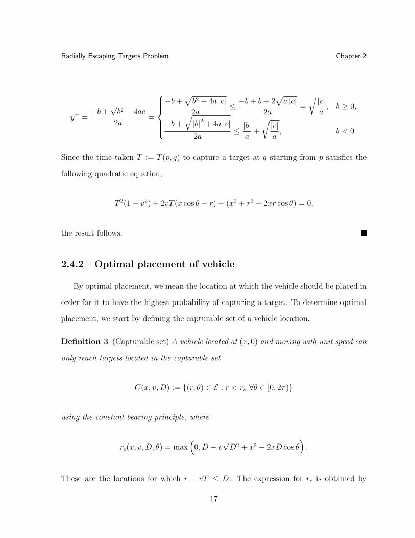
2.4.2 Optimal placement of vehicle
By optimal placement, we mean the location at which the vehicle should be placed in
order for it to have the highest probability of capturing a target. To determine optimal
placement, we start by defining the capturable set of a vehicle location.
Definition 3 (Capturable set) A vehicle located at (x, 0) and moving with unit speed can
only reach targets located in the capturable set
C(x, v,D) := {(r, ✓) 2 E : r < rc 8✓ 2 [0, 2⇡)}
using the constant bearing principle, where
rc(x, v,D, ✓) = max⇣
0, D � vpD2 + x2 � 2xD cos ✓
⌘
.
These are the locations for which r + vT D. The expression for rc is obtained by
17

Radially Escaping Targets Problem Chapter 2
setting rc + vT = D. The radial location rc corresponds to the locations of targets that
the vehicle can capture just before they escape the disk. The probability that a target is
in the capturable set of a particular vehicle location (x, 0) is given by
⇢(x, v,D) :=
R
2⇡
0
R D
0
P [(r, ✓) 2 C(x, v,D)] f(r)e(✓)drd✓R
2⇡
0
R D
0
P [(r, ✓) 2 E ] f(r)e(✓)drd✓=
R
2⇡
0
R rc
0
f(r)e(✓)drd✓
⇡D2
.
When the vehicle is at location p⇤ = (x⇤(v,D), 0) where
x⇤(v,D) := arg max0xD
⇢(x, v,D), (2.1)
the probability of it capturing a target is maximum. The vehicle location x⇤(v,D) is
referred to as the optimal location. Let ⇢⇤(v,D) := ⇢(x⇤, v,D). Closed form expressions
for x⇤ and ⇢⇤ do not appear to be possible for all v 2 (0, 1). However, from numerical
calculations it is known that x⇤ = 0 for v 2 (0, 0.5] irrespective of the value of the
parameter D. The numerically computed variation of x⇤(v,D) and ⇢⇤(v,D) for D = 1 is
shown in Fig. 2.2. For target speed v 0.5, x⇤ = 0 and the vehicle location p⇤ = (0, 0)
maximizes the probability of the vehicle being able to capture a target before it escapes.
For higher speeds, this location is closer to the boundary. There is a qualitative di↵erence
between these two cases. For the former case, p⇤ = (0, 0) is the unique vehicle location
which maximizes ⇢ whereas for the later case, the set of corresponding optimal locations
is all points with radial coordinate equal to x⇤.
Theorem 4 (Capture fraction upper bound) For every policy P for the RET(v,�) prob-
lem, Fcap
(P ) ⇢⇤(v,D).
Proof: Let the vehicle start from x1
and service target at p1
. The probability of
the vehicle capturing this target is maximum when x1
= x⇤. The best case scenario is
18
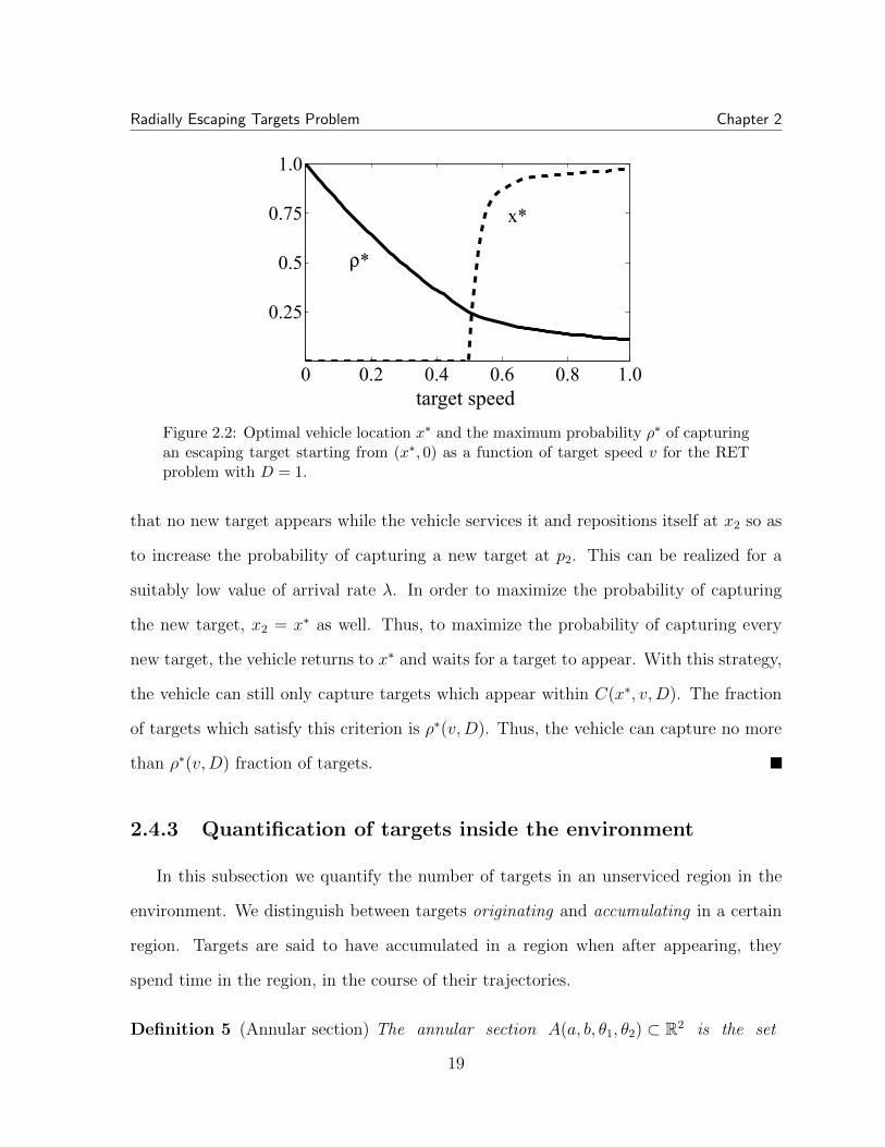
Radially Escaping Targets Problem Chapter 2
0 0.2 0.4 0.6 0.8 1.0
0.25
0.5
0.75
1.0
x*
�*
target speed
Figure 2.2: Optimal vehicle location x
⇤ and the maximum probability ⇢
⇤ of capturingan escaping target starting from (x⇤
, 0) as a function of target speed v for the RETproblem with D = 1.
that no new target appears while the vehicle services it and repositions itself at x2
so as
to increase the probability of capturing a new target at p2
. This can be realized for a
suitably low value of arrival rate �. In order to maximize the probability of capturing
the new target, x2
= x⇤ as well. Thus, to maximize the probability of capturing every
new target, the vehicle returns to x⇤ and waits for a target to appear. With this strategy,
the vehicle can still only capture targets which appear within C(x⇤, v,D). The fraction
of targets which satisfy this criterion is ⇢⇤(v,D). Thus, the vehicle can capture no more
than ⇢⇤(v,D) fraction of targets.
2.4.3 Quantification of targets inside the environment
In this subsection we quantify the number of targets in an unserviced region in the
environment. We distinguish between targets originating and accumulating in a certain
region. Targets are said to have accumulated in a region when after appearing, they
spend time in the region, in the course of their trajectories.
Definition 5 (Annular section) The annular section A(a, b, ✓1
, ✓2
) ⇢ R2 is the set
19

Radially Escaping Targets Problem Chapter 2
A(a, b, ✓1
, ✓2
) := {(r, ✓)|a r b, ✓ 2 [✓1
, ✓2
]}.
Lemma 6 (Accumulated targets in an annular section) For 0 < a < b < D, let nA
be the number of targets accumulated at steady state in an unserviced annular section
A(a, b, 0, 2⇡) and fa(x) be the distribution of the accumulating targets w.r.t the radial
location x 2 [0, D]. Then,
(i) E[nA] = (b3 � a3)�/3vD2,
(ii) Var[nA] = (b3 � a3)�/3vD2 and
(iii) fa(x) = �x2/vD2.
Proof: Firstly, steady state is assumed, meaning that the initial transient has al-
ready passed, hence the time at which the snapshot is taken is t � D/v. Also, by
unserviced, we mean that the vehicle has not serviced targets in the region under con-
sideration for at least time D/v before the time instant under consideration. Let us
examine the number of targets accumulating in the annulus Ar := A(r, r + �r, 0, 2⇡)
due to targets appearing in the annulus R1
:= A(p1
, p1
+�p1
, 0, 2⇡). Let us also assume
that �r and �p are infinitesimal. The intensity of the Poisson arrival process on R1
is
directly proportional to its area and is equal to 2⇡p1
�p1
�/⇡D2 = 2p1
�p1
�/D2.
P[Ar contains n targets originating from R1
]
= P
n targets originated from R1
in time interval
t, t+�r
v
��
= P
n targets originated from R1
in time interval of length�r
v
�
= exp
✓
�2p1
�p1
��r
D2v
◆
✓
2p1
�p1
��r
D2v
◆n
n!,
20

Radially Escaping Targets Problem Chapter 2
where t = (r � p1
)/v. Thus, the process of targets accumulating in Ar due to targets
originating in R1
is spatially Poisson with intensity area(R1
)/(⇡D2)�/v = 2p1
�p1
�/D2v.
Next, let us examine the process of accumulation of targets in Ar due to two annuli
R1
:= A(p1
, p1
+�p1
, 0, 2⇡) and R2
:= A(p2
, p2
+�p2
, 0, 2⇡).
P[Ar contains n targets from R1
[R2
] =nX
i=0
"
exp
✓
�2p1
�p1
��r
D2v
◆
✓
2p1
�p1
��r
D2v
◆i
i!
⇥ exp
✓
�2p2
�p2
��r
D2v
◆
✓
2p2
�p2
��r
D2v
◆
(n�i)
(n� i)!
#
=exp
✓
�2(p1
�p1
+ p2
�p2
)��r
D2v
◆
⇥
✓
2(p1
�p1
+ p2
�p2
)��r
D2v
◆n
n!(2.2)
Thus the process of targets accumulating in Ar due to targets originating in R1
[R2
is
also spatially Poisson and the intensity of this process, given by (2p1
�p1
+2p2
�p2
)�/D2v =
(area(R1
) + area(R2
))/(⇡D2)�/v, is the sum of the intensities due to R1
and R2
. This
can be extended to all the rings of radii p 2 [0, r]. So arrival process of all targets accu-
mulating in Ar is also spatially Poisson and has intensity area(A(0, r, 0, 2⇡))/(⇡D2)�/v =
(r2�/vD2). Thus the expected number as well as the variance of targets accumulating in
the unserviced annulus Ar is r2��r/vD2.
Next, consider an annular section A(a, b, 0, 2⇡). Since Poisson processes are additive,
the arrival process of targets accumulating in A(a, b, 0, 2⇡) is Poisson and is the sum of
processes of targets accumulating in disjoint annuli like Ar with r 2 [a, b]. Hence the
21
Radially Escaping Targets Problem Chapter 2
vT(X,0)
T
s1 >=(1-v)T
s2 =vT
s3 <=T
s
m
(a) (b)
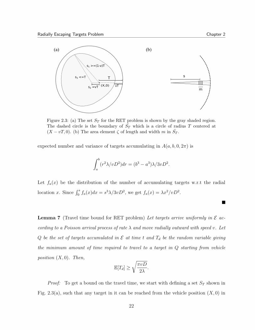
Figure 2.3: (a) The set ST for the RET problem is shown by the gray shaded region.The dashed circle is the boundary of ST which is a circle of radius T centered at(X � vT, 0). (b) The area element ⇣ of length and width m in ST .
expected number and variance of targets accumulating in A(a, b, 0, 2⇡) is
Z b
a
(r2�/vD2)dr = (b3 � a3)�/3vD2.
Let fa(x) be the distribution of the number of accumulating targets w.r.t the radial
location x. SinceR s
0
fa(x)dx = s3�/3vD2, we get fa(x) = �x2/vD2.
Lemma 7 (Travel time bound for RET problem) Let targets arrive uniformly in E ac-
cording to a Poisson arrival process of rate � and move radially outward with speed v. Let
Q be the set of targets accumulated in E at time t and Td be the random variable giving
the minimum amount of time required to travel to a target in Q starting from vehicle
position (X, 0). Then,
E[Td] �r
⇡vD
2�.
Proof: To get a bound on the travel time, we start with defining a set ST shown in
Fig. 2.3(a), such that any target in it can be reached from the vehicle position (X, 0) in
22

Radially Escaping Targets Problem Chapter 2
T time units or less. Mathematically,
ST :=�
(r, ✓) 2 E|X2 + (r + vT )2 � 2X(r + vT ) cos(✓) T 2
.
Also, let ST := {(r, ✓) 2 E|(X � vT � r cos ✓)2 + (r sin ✓)2 T 2}. Since the relative ve-
locity of any target with respect to the vehicle is more than or equal to (1 � v), the
distance s1
of any point on the boundary of ST from (X, 0) is greater than or equal to
T (1� v). Using the triangle inequality, the distance s2
of that point from (X � vT, 0) is
less than or equal to T . Then, ST ✓ ST .
If Td is the random variable giving the minimum amount of time to go from vehicle
location (X, 0) to a target, then Td > T if ST is empty and P[Td > T ] = P[|ST | = 0].
Here, the notation |ST | is used to denote the number of outstanding targets in the set
ST . Further,
P[|ST | = 0] = P[|ST | = 0]P[|ST\ST | = 0] P[|ST | = 0]. (2.3)
We now calculate the probability that an infinitesimal area element ⇣ of length m and
width m centered at (s, 0) shown in Fig. 2.3(b) is empty:
P[|⇣| = 0] = exp
✓
��mv
1
⇡D2
Z s
0
r✓dr
◆
= exp
✓
��mv
1
⇡D2
Z s
0
rm
sdr
◆
(2.4)
= exp
✓
�m2
v
�s
2⇡D2
◆
� exp
✓
�m2�
2⇡vD
◆
= exp
✓
��2⇡vD
area(⇣)
◆
, (2.5)
where the inequality follows from the fact that s 2 [0, D], and the exponential function
has a minimum at s = D. The last equality is true since area(⇣) = m2. Further, every
23

Radially Escaping Targets Problem Chapter 2
compact set can be written as a countable union of non-overlapping rectangles. Thus,
Eq. (2.4) holds for the compact measurable set ST as well. Then, using the results from
Eq. (2.3) and Eq. (2.4),
P[|ST | = 0] � P[|ST | = 0] � exp
✓
��2⇡vD
area(ST )
◆
= exp
✓
��2⇡vD
⇡T 2
◆
,
and the expectation of Td can be bounded as follows:
E[Td] =
Z
+1
0
P[Td > T ]dT =
Z
+1
0
P[|ST | = 0] �Z
+1
0
P[|ST | = 0]dT
�Z
+1
0
exp
✓
�T 2�
2vD
◆
dT �p⇡
2
r
2vD
�=
r
⇡vD
2�.
so the result is obtained.
Theorem 8 (Policy Independent Upper Bound on Service Fraction) An upper bound on
the service fraction of any policy P for the RET problem satisfies
Fcap
(P ) r
2
⇡v�D.
Proof: This follows from the fact that in order to service a fraction c 2 (0, 1] of
targets, we require that the rate at which targets are serviced is more than the rate at
which they arrive [60], i.e., c�E[T ] 1. Since T > Td, the result now follows by using
Lemma 7.
2.4.4 Bounds on paths and tours through targets
To distinguish static targets from moving targets, we introduce some terminology. A
target moving radially outward is referred to as an escaping target. A target is said to
have been ‘captured’ by the vehicle if the vehicle reaches the target before it escapes the
24

Radially Escaping Targets Problem Chapter 2
environment. The following results are used to estimate and bound the length of the
path through targets in the environment.
Theorem 9 (Upper bound on path through escaping targets) Let targets starting from
(ri, ✓i), i 2 {1, . . . , N} move radially outward with speed v. Let T be the length of the path
through these escaping targets in some arbitrary order � : {1, . . . , N}! {1, . . . , N}. Let
Ts be the length of the path through static targets located at (ri + vT , ✓i), i 2 {1, . . . , N}
processed in order � and T � T . Then,
T Ts
1� v.
Proof: Without loss of generality, let the targets be labeled in the order in which
they are processed. Let the vehicle take time Tj to service the j�th escaping target having
serviced the (j� 1)�th escaping target. Consider the i�th escaping target starting from
(ri, ✓i). The vehicle services this target at timePi
j=1
Tj. It then starts for the escaping
target i+1 and reaches it in time Ti+1
. Let T0i+1
be the distance between (ri+vPi+1
j=1
Tj, ✓i)
and (ri+1
+ vPi+1
j=1
Tj, ✓i+1
). Also, let T00i+1
be the distance between (ri + vT, ✓i) and
(ri+1
+ vT, ✓i+1
) while Ts,i+1
is the distance between (ri + vT , ✓i) and (ri+1
+ vT , ✓i+1
).
Since the distance between two targets moving radially outward with the same speed is
a non-decreasing function of time, T0i+1
T00i+1
Ts,i+1
. Referring to Fig. 2.4, from the
triangle inequality, T0i+1
+ vTi+1
� Ti+1
, i.e., Ti+1
(T0i+1
)/(1 � v) (Ts,i+1
)(1 � v).
Extending this to all the targets in the path,
T =nX
i=1
Ti+1
nX
i=1
Ts,i+1
1� v=
Ts
1� v.
The upper bound on the length of the path through escaping targets is thus related
25
Radially Escaping Targets Problem Chapter 2
r1
r2
T 0, i+1
T i+1T' i+1 T" i+1
T s, i+1
i
i+1
v∑ j=1i T j
v∑ j=1i+1 T j
vT i+1
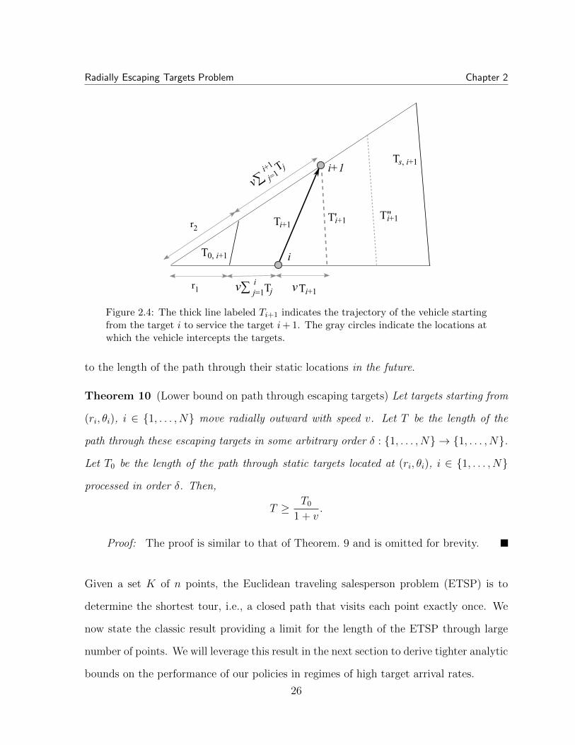
Figure 2.4: The thick line labeled Ti+1
indicates the trajectory of the vehicle startingfrom the target i to service the target i + 1. The gray circles indicate the locations atwhich the vehicle intercepts the targets.
to the length of the path through their static locations in the future.
Theorem 10 (Lower bound on path through escaping targets) Let targets starting from
(ri, ✓i), i 2 {1, . . . , N} move radially outward with speed v. Let T be the length of the
path through these escaping targets in some arbitrary order � : {1, . . . , N}! {1, . . . , N}.
Let T0
be the length of the path through static targets located at (ri, ✓i), i 2 {1, . . . , N}
processed in order �. Then,
T � T0
1 + v.
Proof: The proof is similar to that of Theorem. 9 and is omitted for brevity.
Given a set K of n points, the Euclidean traveling salesperson problem (ETSP) is to
determine the shortest tour, i.e., a closed path that visits each point exactly once. We
now state the classic result providing a limit for the length of the ETSP through large
number of points. We will leverage this result in the next section to derive tighter analytic
bounds on the performance of our policies in regimes of high target arrival rates.
26

Radially Escaping Targets Problem Chapter 2
Theorem 11 (Asymptotic ETSP length,[96]) If a set K of n points is distributed inde-
pendently and identically in a compact set Q, then there exists a constant � such that
limn!+1
ETSP (K)pn
= �
Z
Q
'(q)1/2dq,
where ' is the density of the absolutely continuous part of the point distribution.
The constant � has been estimated numerically as � ⇡ 0.7120± 0.0002 [81].
2.5 Policies
In this section, we propose three policies for the RET problem. The SAC policy is
designed for low target arrival rates while the SW policy is designed for moderate target
arrival rates. Finally, the SNB policy is proposed for high arrival rates.
2.5.1 Stay at Center (SAC) Policy
According to this policy, the vehicle stays at the optimal location in the disk and
waits for new targets to appear in its capturable set. For v 2 [0, 0.5], this location is
the center. The SAC policy is suitable for low target arrival rates at which the optimal
vehicle location takes prominence.
Given a vehicle location (x, 0) 2 E , recall that C(x, v,D) denotes the capturable set
for the vehicle. Let x⇤ and ⇢⇤ be defined as per Eq. (2.1). The formal description of the
SAC policy is given in Algorithm 1.
Algorithm 1 has the following guarantee on capture fraction.
Theorem 12 (SAC Policy Capture Fraction) The capture fraction of the SAC policy
27
Radially Escaping Targets Problem Chapter 2
Algorithm 1: Stay At Center (SAC) policy
Given: v, D known and the vehicle placed at (x⇤, 0).1 Intercept a target that appears inside C(x⇤, v,D);2 Return back to (x⇤, 0);3 Repeat from step 1.
satisfies
Fcap
(SAC) � ⇢⇤(v,D)
2⇢⇤(v,D)�D + 1.
If v 2 [0, 0.5] so that the optimal vehicle location x⇤ = 0, then the above fraction
becomes equal to
Fcap
(SAC) � (1� v)2
2�(1� v)2D + 1.
Proof: See Appendix.
Remark 13 (Optimality in light load, i.e., �! 0+) In the light load regime of �! 0+,
the capture fraction achieved equals ⇢⇤(v,D), which is exactly equal to the probability that
a target falls within the capturable set C when the vehicle is located at the optimal location
(x⇤, 0). Comparing with Theorem 4, we see that the SAC policy is optimal in this limiting
regime.
2.5.2 Sector-wise (SW) Policy
In the Sector-wise policy, the vehicle stays closer to the boundary and utilizes the
high relative velocity of the outgoing targets. It starts every iteration at a radial location
X and services the first target with the smallest clockwise angular separation in a specific
subset associated with the iteration.
One such subset J1
which the vehicle encounters in the first iteration is shown by the
shaded region in Fig. 2.5. It then proceeds to the nearest location with radial coordinate
X in the disk and waits for a specified time to begin its next iteration. The formal
28

Radially Escaping Targets Problem Chapter 2
3 3
3
4 4 4
4
4
4
5 5 5 5
5
5
5
5
6
6
6
6
6 6 6 6
7
7
7
7
7
7 7 7 7
8
8
8 8 8 89 9 9 910 10 10
arrival rate
targ
et sp
eed
5 10 15 20 25 300.2
0.3
0.4
0.5
0.6
0.7
0.8
0.9(a) (b)
X
θ
vθ =0
Xcosθ
D
Figure 2.5: (a) Vehicle located at p = (X, 0) services outstanding targets shown bythe shaded region. (b) Factor of optimality of the SW policy in di↵erent parameterregimes v, � when D = 1.
Algorithm 2: Sector-wise (SW) policy
Given: v,D known and the vehicle placed at (X, 0).1 Set X = D
p1� v2, W = max (0, X(1/4v �
p2));
2 repeat3 if there are targets in E with clockwise angular separation ✓ < ⇡/2 such that
their radial coordinate r satisfies r X cos ✓ then4 Service the target with smallest angular separation and move to nearest
location in E with radial coordinate X ;5 Wait for time W and return to step 3.6 else7 Stay at current location.8 end
9 until all targets are serviced or have escaped ;
description of the policy is given in Algorithm 2. While the SW policy is applicable in all
parameter regimes of the RET problem, for a fixed speed v, it is constant factor optimal
in moderate arrival regimes as established in Theorem 15. Algorithm 2 has the following
guarantee on capture fraction.
Lemma 14 (SW Policy Capture Fraction) The capture fraction of the SW policy satisfies
Fcap
(SW) � 1
�
✓
W +⇡D
4(3⌘
1
(k) + ⌘
2
(k)) +8
�(1� v
2)⌘
3
(k)
◆�1
,
29

Radially Escaping Targets Problem Chapter 2
where
⌘1
(k) = (L�1
(8k)� I1
(8k)� L�1
(20k) + I1
(20k)) , (2.6)
⌘2
(k) = (I0
(8k)� L0
(8k)� I0
(20k) + L0
(20k)) , (2.7)
⌘3
(k) = 1� ⇡/2 (I0
(12k)� L0
(12k)� I0
(20k) + L0
(20k)) , (2.8)
W = max (0, Dp1� v2(1/4v �
p2)), k = �D(1�v2)3/2/72⇡v, and I
0
and I1
are modified
Bessel functions of the first kind and L0
and L�1
are modified Struve functions [1].
Proof: See Appendix.
Theorem 15 (Performance in moderate arrival rates) For � > 7⇡v(1�v2)3/2D
and v 2
(1/4p2, 1), the capture fraction of the SW policy satisfies
Fcap
(SW) � ↵(v)
r
2
⇡v�D,
where
↵(v) =
pv
⇡2
✓
v
(1� v2)3/2
◆
1/2
+10
3
(1� v2)1/2
v
!�1/2
. (2.9)
Proof: See Appendix.
Thus, for moderate arrival rates and v 2 (1/4p2, 1), using the result from Theorem 15
and the fundamental bound obtained in Theorem 8, the SW policy is also a constant
factor policy with the factor equal to 1/↵(v).
2.5.3 Stay-Near-Boundary (SNB) Policy
We now introduce the SNB policy for the high arrival regime. In this regime, the
density of targets accumulating close to the boundary of the disk is high. Hence, the
distance traversed by the vehicle (and the time taken) between capturing consecutive
30

Radially Escaping Targets Problem Chapter 2
targets is small. Consequently, the distance by which the targets move between consec-
utive captures is also small. Hence, the vehicle can plan ahead and capture multiple
targets in a single iteration. To determine the order of captures, it uses the solution
to the Euclidean Minimum Hamiltonian Path (EMHP) problem which can be stated as
follows:
Given a set of n (stationary) points, determine the length of the shortest path
which visits each point exactly once.
The SNB policy makes use of three parameters g, h and ncap
. At the beginning of
every iteration, the vehicle computes an EMHP through the locations that the targets
accumulated in A(g, h, 0, 2⇡) will have after time (D � h). This is done to levarage the
result from Theorem 9. It uses the order obtained from the EMPH to service the first
ncap
targets using constant bearing principle. A formal statement of the SNB policy is
given in Algorithm 3.
The parameters g, h and ncap
are chosen in a way which ensures that the vehicle will
service all the ncap
targets accumulated in A(g, h, 0, 2⇡) at the beginning of the iteration
before the last target escapes the environment. This can be achieved in the following
way:
(i. parameters g and h are solutions to variables a and b respectively in the following
31
Radially Escaping Targets Problem Chapter 2
Optimization Problem:
maxa,b
✓
b3 � a3
b2 � a2
◆
subject to
µA =�(b3 � a3)
3vD2
,
�
1� v
r
6⇡
b3 � a3
✓
b2 � a2
2
◆
p
µA(1 + v) D � b
v,
�
1 + v
r
6⇡
b3 � a3
✓
b2 � a2
2
◆
p
µA(1� v) � b� a
v,
0 a < b < D.
(ii. parameter ncap
is set as follows:
ncap
:=�(1� v)
3vD2
(h3 � g3).
Algorithm 3 has the following guarantee on the capture fraction of the RET problem.
Algorithm 3: Stay-Near-Boundary (SNB) policy
Given: g, h and ncap
are known and the vehicle is at (h, 0).1 if A(g, h, 0, 2⇡) contains outstanding targets then2 s
1
:= set of locations of outstanding targets in A(g, h, 0, 2⇡);3 s
2
:= set of their locations if they move radially outward by distance (D � h);4 := order of the EMHP starting from (D, 0), visiting targets in s
2
and endingat (D, 0);
5 service the first ncap
targets in s1
in order from using constant bearingprinciple and return to (h, 0).
6 end
Theorem 16 (SNB Policy Capture Fraction) For any fixed v 2 (0, 1), in the limit as
32

Radially Escaping Targets Problem Chapter 2
�! +1, the capture fraction of the SNB policy satisfies
Fcap
(SNB) � 2p
7�
r
2
⇡�vD
with probability one, where
p := p(D) =
8
>
>
<
>
>
:
1, D > 1,
5pD
6, otherwise.
Proof: See Appendix.
Corollary 17 (Performance of the SNB policy) In the limit as � ! +1 such that
� > (1 + v)2/2⇡�2v(1� v), the SNB policy is within a factor 7�/2p of the optimal. For
D � 1, this factor is ⇡ 2.52.
2.6 Simulations
The numerical performance of the SAC and SW policies for arrival rates of � = 2 and
� = 10 respectively and all target speeds is shown in Fig. 2.6. The parameter D = 1 for
these simulations. The mean of the capture fraction based on 1000 simulations is shown
along with its standard deviation. It agrees well with the theoretical lower bounds.
The theoretical bounds are still conservative. For the SAC policy, the conservativeness
comes from the application of Jensen’s inequality in Eq. (2.10). For the SW policy, the
conservativeness of the bound is because of inequalities introduced in Eq. (2.11),(2.13)
to bound integrals.
33

Radially Escaping Targets Problem Chapter 2
0.2 0.4 0.6 0.80
0.2
0.4
0.6
0.8
SAC policy, arrival rate = 2
target speed
capt
ure
frac
tion
0.2 0.4 0.6 0.80
0.1
0.2
0.3
0.4
0.5
SW policy, arrival rate = 10
target speed
capt
ure
frac
tion theoretical
experimentalfundamental
theoreticalexperimentalfundamental
(a) (b)
Figure 2.6: Performance of the (a) SAC and (b) SW policies for arrival rates � = 2and � = 10 respectively for the RET problem with D = 1. The theoretical boundsare from Theorem 12 and Theorem 15 respectively.
Appendix
Proof of Theorem 12: Notice that if mcap
(t) > 0 for some t > 0, then
lim supt!+1
Eh
mcap(t)
mcap(t)+mmiss(t)
i
= lim supt!+1
E
1
1+
mmiss(t)mcap(t)
�
�✓
1 + lim supt!+1
Eh
mmiss(t)mcap(t)
i
◆�1
,
(2.10)
where the last step comes from an application of Jensen’s inequality [21]. Thus, we can
determine a lower bound on the capture fraction by studying the number of targets that
escape per captured target. Consider a tagged target i which falls within C(x⇤, v,D). The
time ti taken by vehicle to intercept target i and return to the optimal location satisfies
ti 2D. Therefore, the number of targets that escape because the vehicle intercepts the
i-th target is equal to the sum of 1) the number of targets that arrive anywhere in the
environment during the time interval of ti and 2) the number of targets that are generated
outside of C(x⇤, v,D) while the vehicle is waiting for the next capturable target. Since the
target arrival process is temporally Poisson, the expected number of targets in case 1 are
given by �ti 2�D. The spatial distribution of the targets is uniform random. Further,
area(C(x⇤, v,D)) = ⇢⇤(v,D)⇡D2. Therefore, the targets missed in case 2, denoted by
34

Radially Escaping Targets Problem Chapter 2
Nmiss
is a random variable distributed as follows.
Nmiss
=
8
>
>
>
>
>
>
>
>
>
>
>
>
>
>
>
>
>
>
<
>
>
>
>
>
>
>
>
>
>
>
>
>
>
>
>
>
>
:
0, with probability ⇢⇤(v,D),
1, with probability ⇢⇤(v,D)⇣
1� ⇢⇤(v,D)⌘
,
2, with probability ⇢⇤(v,D)⇣
1� ⇢⇤(v,D)⌘
2
,
...
k, with probability ⇢⇤(v,D)⇣
1� ⇢⇤(v,D)⌘k
,
...
Therefore,
E [Nmiss
] =1X
k=1
k⇢⇤(v,D)⇣
1� ⇢⇤(v,D)⌘k
= ⇢⇤(v,D)1X
k=1
⇣
1� ⇢⇤(v,D)⌘k
= ⇢⇤(v,D)1� ⇢⇤(v,D)
(⇢⇤(v,D))2=
1
⇢⇤(v,D)� 1.
Substituting the upper bound for case 1 and the expression for case 2 in (2.10), we obtain
Fcap
(SAC) � 1
2�D + 1
⇢⇤(v,D)
=⇢⇤(v,D)
2⇢⇤(v,D)�D + 1.
Proof of Theorem 14: In the sector-wise policy, the vehicle starts every iteration at a
distance X = Dp1� v2 from the center. If ✓v is the angular position of the vehicle in
its i-th iteration and
Ji := {(r, ✓) | 0 r X cos(✓ � ✓v), ✓ � ✓v 2 [0, ⇡/2]} ,
then if there is an outstanding target in Ji, the vehicle services the target in Ji with the
smallest angular separation from ✓v in the counterclockwise direction. The choice of X
35

Radially Escaping Targets Problem Chapter 2
ensures that the vehicle always services any target in Ji before it escapes the disk.
We now calculate the expectation of the time required for a single iteration of the
SW policy. Without loss of generality we assume that i = 1, ✓v = 0 initially and the
vehicle is at (X, 0). We also assume that the environment is unserviced. Let K(�1
, �2
) :=
{(r,�)|0 r X cos�,� 2 [�1
, �2
]} for �1
< �2
. Also, for infinitesimal �✓, let ✓+ = ✓+�✓.
Then the probability of the first outstanding target in J1
being at an angular location ✓,
i.e.
P[first target is in K(✓, ✓+)| J1
is not empty ] =P [|K(0, ✓)| = 0]P⇥
|K(0, ✓+)| 6= 0⇤
=exp (�k (9 sin ✓ + sin 3✓))
⇥�
1� exp�
�k�
9 sin ✓+ + sin 3✓+���
� exp(�8k sin ✓) (1� exp(�12k sin ✓)) ,
(2.11)
where k = �X3
72⇡vD2 . A number of results are used to obtain Eq. (2.11). The first result,
which is derived in the same spirit as Eq. (2.4), is that for ↵ 2 [0, 2⇡],
P [|K(0,↵)| = 0] = exp (�k (9 sin↵ + sin 3↵)) . (2.12)
The second supporting result is the following empirically obtained inequality for ↵ 2
[0, ⇡/2]: 12 sin↵ � 9 sin↵ + sin 3↵ � 8 sin↵.
Now that we have an expectation of the first target being at an angular location
✓ relative to the vehicle, we calculate the time taken to capture this target. Let T✓
be the random variable denoting the time taken to start from (X, 0), service a target
at (r, ✓) and go to (X, ✓) to start the next iteration. We determine a bound on the
expectation of T✓. Once again, we assume that the environment is unserviced and note
36

Radially Escaping Targets Problem Chapter 2
that the probability distribution of the outstanding targets is given by fa(r) = �r2/vD2
as obtained in Lemma 6. Since r X cos ✓, we use Lemma 2 to obtain a lower bound
on the expectation of T✓:
E[T✓] 2
R
X cos ✓
r=0
✓
�r2
vD2
◆✓
pX2 + r2 � 2Xr cos ✓p
1� v2
◆
drR
X cos ✓
r=0
✓
�r2
vD2
◆
dr
=
2
R
cos ✓
s=0
X
✓
�s2
vD2
◆✓
p1 + s2 � 2s cos ✓p
1� v2
◆
dsR
cos ✓
s=0
✓
�s2
vD2
◆
ds
(2.13)
6Xp1� v2
✓
sin ✓
4+
1
12
◆
=: �(✓). (2.14)
The factor of two is required since the vehicle has to go to (X, ✓) to start the next
iteration and the time required for this is always less than or equal to the time required
to service the target at (r, ✓) starting from (X, 0). If T is the random variable denoting
the time required to start from (X, 0), service the first target in J1
and return to the
radial location X, then using the result from Eq. (2.11),
E[T |J1
is not empty] =
Z ⇡/2
✓=0
E[T✓] P[ first target in K(✓, ✓+)]d✓
Z ⇡/2
✓=0
�(✓) (exp(�8k sin ✓) (1� exp(�12k sin ✓))) d✓
=
✓
6Xp1� v2
◆
⇣⇡
8⌘1
(k) +⇡
24⌘2
(k)⌘
. (2.15)
(2.16)
where the functions ⌘1
and ⌘2
are as defined in Eq. (2.6). Further, using the result from
37
Radially Escaping Targets Problem Chapter 2
Eq. (2.12),
P[ J1
is empty ] 1�Z ⇡/2
0
exp(�12k sin ✓) (1� exp(�8k sin ✓)) d✓
=1� ⇡
2(I
0
(12k)� L0
(12k)� I0
(20k) + L0
(20k))
=⌘3
(k), (2.17)
and the expected time that the vehicle has to wait for a new target to appear in J1
is
less than 8/�(1 � v2) since the area of J1
is (1 � v2)/8 times the area of the disk. This
is in addition to the time W that the vehicle waits at the beginning of the iteration. So,
using Eq. (2.15) and Eq. (2.17), the time T taken to finish a single iteration of the SW
policy has the following expectation:
E[T ] =W + E[T | J1
is not empty ] + E[T | J1
is empty ]
=W + E[T | J1
is not empty ] +8
�(1� v2)P[ J
1
is empty ]
W +
✓
6Xp1� v2
◆
⇣⇡
8⌘1
(k) +⇡
24⌘2
(k)⌘
+
✓
8
�(1� v2)
◆
⌘3
(k)
=W +3⇡D
4⌘1
(k) +⇡D
4⌘2
(k) +8
�(1� v2)⌘3
(k).
Then, Fcap
(SW ) � 1/�E[T ]. Finally, in the most favorable scenario for the vehicle, it
intercepts each new target at the end of each quadrant at a radial location X, waits for
time W and begins a new iteration. The time in which it returns to a quadrant in this
manner is equal to 4p2X +4W . Since X/v < 4
p2X +4W for all v < 1, the assumption
that the vehicle always begins an iteration in an unserviced region holds true.
Proof of Theorem 15: From Lemma 14, we know that the capture fraction of the SW
38

Radially Escaping Targets Problem Chapter 2
policy satisfies
Fcap
(SW) � 1
�
✓
W +⇡D
4(3⌘
1
(k) + ⌘2
(k)) +8
�(1� v2)⌘3
(k)
◆�1
. (2.18)
When v > 1/4p2, W = 0. Further, when � > 7⇡v
(1�v2)3/2D, k = �(1�v2)3/2
72⇡v> 0.1. Using
upper and lower bounds on Bessel and Struve functions, the following hold true for
k > 0.1,
3
4⌘1
(k) +1
4⌘2
(k) =3
4(L�1
(8k)�I1
(8k)� L�1
(20k) + I1
(20k))
+1
4(I
0
(8k)� L0
(8k)� I0
(20k) + L0
(20k)) 1
12pk,
(2.19)
⌘3
(k) = 1� ⇡
2(I
0
(12k)� L0
(12k)� I0
(20k) + L0
(20k)) 5pk
2. (2.20)
Using Eq. 2.19 and 2.20, and the result in Eq. 2.18, Fcap
(SW) can be bounded and
the result is obtained.
Proof of Theorem 16 We start with calculating an upper bound on the length of the
tour through all the targets in A(g, h, 0, 2⇡). Let Q := {(r, ✓) 2 A(g, h, 0, 2⇡)} be the set
of locations of targets accumulated in A(g, h, 0, 2⇡) and n = |Q|. From Lemma 6, the
normalized distribution of these targets w.r.t the radial location x is given by fn(x) =
3x2/(h3 � g3) for x 2 [g, h]. Let Q be the set of locations (s,�) of these targets if
they move outwards by distance d and occupy A(g + d, h + d, 0, 2⇡). The normalized
distribution functions of the random variables s and � which denote locations of these
39

Radially Escaping Targets Problem Chapter 2
targets are
fs(x) =3(x� d)2
h3 � g3and e�(y) =
1
2⇡.
Using Theorem 11 and assuming that n!1 (which we will revisit later),
limn!+1
ETSP (Q)pn
= �
r
6⇡
h3 � g3
✓
h2 � g2
2
◆
with
'(s,�) = fs(x)e�(y) =3(x� d)2
(h3 � g3)
1
2⇡.
Using Chebyshev’s inequality, if µA and �A are the mean and standard deviation of the
random variable n, then for any fixed v 2 (0, 1),
P[n < µA(1 + v)] � 1� �2
A/v2µ2
A.
Then, the condition
tu :=�
1� v
r
6⇡
h3 � g3
✓
h2 � g2
2
◆
p
µA(1 + v) D � g
v(2.21)
from the Optimization Problem (i ensures that the n targets will be serviced before they
escape the disk with at least a probability of 1��2
A/v2µ2
A. Similarly since ncap
= µA(1�v)
and v > 0,
P[n > µA(1� v)] � 1� �2
A/v2µ2
A (2.22)
so that n > ncap
and the vehicle services ncap
targets in an iteration with probability of
at least 1� �2
A/v2µ2
A. Further, the condition
�
1 + v
r
6⇡
h3 � g3
✓
h2 � g2
2
◆
p
µA(1� v) � h� g
v(2.23)
40

Radially Escaping Targets Problem Chapter 2
from the Optimization Problem (i ensures that with probability of at least 1� �2
A/v2µ2
A,
when the vehicle starts an iteration, A(g, h, 0, 2⇡) is unserviced. In the above inequality,
the left-hand side is the lower bound on the length of the tour through µA(1� v) targets
in A(g, h, 0, 2⇡) obtained by using Theorem 10. We also know that
µA =�(h3 � g3)
3vD2
and �2
A = µA from Lemma 6. When � ! +1 and v 2 (0, 1), then µA ! +1 and
ncap
! +1 so that Eq. (2.21),(2.22) and (2.23) hold true with probability one. Then,
since ncap
! +1 and n > ncap
with probability one, our earlier assumption that n! +1
is true as well.
If ktot
(i) and kcap
(i) are the number of targets that have appeared and have been
serviced in the i�th iteration of the SNB policy, and Fi
(SNB) = E [kcap
(i)/ktot
(i)], then
since at every iteration, kcap
(i) � ncap
,
Fi
(SNB) � E
ncap
ktot
(i)
�
= ncap
E
1
ktot
(i)
�
� ncap
E[ktot
(i)], (2.24)
where the last inequality holds true using Jensen’s inequality for convex function 1/ktot
(i).
Next, when � > (1 + v)2/2⇡�2v(1� v), the solution to the Optimization Problem (i
exists and the parameters g and h obtained by solving it satisfy
h3 � g3
h2 � g2� 4Dp
7
1� vp1 + v
.
Now, when � ! +1, for a fixed speed, the above condition on � is met. Then, from
Eq. 2.24 and using the fact that E[ktot
(i)] �tu,
Fi
(SNB) � 2p(1� v)2
7(1 + v)
1� v
�
r
2
⇡�v.
41

Radially Escaping Targets Problem Chapter 2
Let the countably infinite set Y := {Fi
(SNB) 8i 2 N}. Also, let the uncountable set
Z := {E [mcap
(t)/mtot
(t)] 8t 2 R�0
} . Since Y ✓ Z,
Fcap
(SNB) = lim supt!1
E
mcap
(t)
mtot
(t)
�
� lim supi!1
Fi
(SNB) � 2p(1� v)2
7(1 + v)
1� v
�
r
2
⇡�v,
the result is obtained.
42

Chapter 3
Robotic Surveillance:
Detection of Intruder Location
In this chapter we study a surveillance problem in which unknown intruder locations have
to be detected in networked environments. This is achieved by designing Markov chain
random walks for the surveillance vehicle which have minimum mean first passage time.
Motivating examples for this problem include the monitoring of oil spills [29], the detec-
tion of forest fires [57], the tracking of border changes [97], and the periodic patrolling
of an environment [39, 76]. Other applications include minimizing emergency vehicle
response times [14] as well as servicing tasks in robotic warehouse management [106].
In areas of research outside of robotics, the study of the mean first passage time is
of general mathematical and engineering interest. Similar to the fastest mixing Markov
chain, the mean first passage time is a metric by which to gauge the performance of
a random walk. The mean first passage time is also potentially useful in determining
how quickly information propagates in an online network [9] or how quickly an epidemic
spreads through a contact network [105].
43

Robotic Surveillance: Detection of Intruder Location Chapter 3
3.1 Contributions
The contributions of this chapter 1 are as follows. First, we provide a convex opti-
mization framework to minimize the Kemeny constant of a reversible Markov chain given
the underlying graph topology of the random walk and the desired stationary distribu-
tion. Second, we extend the formulation of the mean first passage time to the network
environments with non-homogeneous travel times, a generalization not yet looked at in
the literature. We denote this extension the weighted Kemeny constant. Third, we derive
a closed form solution for the weighted Kemeny constant and show its relation to the
Kemeny constant. Fourth, we provide a convex optimization framework to minimize the
weighted Kemeny constant of a Markov chain with desired stationary distribution. Fifth,
we provide a semidefinite program (SDP) formulation for the optimization of the Kemeny
constant and the weighted Kemeny constant. Finally, we look at two stochastic surveil-
lance scenarios; in the first scenario we provide a setup in which minimizing the weighted
Kemeny constant leads to the optimal Markov-chain strategy. In the second surveil-
lance scenario we establish through numerical simulation that the Markov chain with the
minimum weighted Kemeny constant performs substantially better compared with other
well-known Markov chains like the the fastest mixing chain and the Metropolis-Hastings
Markov chain.
3.2 Organization
We state the contributions of the chapter is Section 3.1. We then summarize the
notation which we use throughout this chapter and the next. We also briefly review
properties of Markov chains. In Section 3.3 we give background for the Kemeny constant
and present our results for its minimization. In Section 3.4 we introduce and provide
1This is joint work with Rushabh Patel
44

Robotic Surveillance: Detection of Intruder Location Chapter 3
detailed characterization of the weighted Kemeny constant as well as its minimization.
In Section 3.5 we provide practical surveillance applications of the weighted Kemeny
constant. In the final Section we present our conclusions and future research directions.
Notation
We use the notation A = [aij] to denote a matrix A with the element aij in its i-th
row and j-th column and, unless otherwise indicated, use bold-faced letters to denote
vectors. Letting �ij denote the Kronecker delta, Ad
= [�ijaij] represents the diagonal
matrix whose diagonal elements are the diagonal elements of the matrix A. The column
vector of all ones and length n is denoted by n 2 Rn⇥1 and I represents the identity
matrix of appropriate dimension. We use diag[b] to denote the diagonal matrix generated
by vector b and Tr[A] to denote the trace of matrix A.
Properties of Markov chains
A Markov chain is a sequence of random variables taking value in the finite set
{1, . . . , n} with the Markov property, namely that, the future state depends only on the
present state; see [50, 55] for more details. Let Xk 2 {1, . . . , n} denote the location of a
random walker at time k 2 {0, 1, 2, . . . }. Some terminology for Makov chains follows:
(1) A Markov chain is time-homogeneous if P[Xn+1
= j|Xn = i] = P[Xn = j|Xn�1
=
i] = pij, where P 2 Rn⇥n is the transition matrix of the Markov chain.
(2) The vector ⇡ 2 Rn⇥1 is a stationary distribution of P ifPn
i=1
⇡i = 1, 0 ⇡i
1 for all i 2 {1, . . . , n} and ⇡
TP = ⇡
T .
(3) A time-homogeneous Markov chain is said to be reversible if ⇡ipij = ⇡jpji, for
all i, j 2 {1, . . . , n}. For reversible Markov chains, ⇡ is always a steady state
45

Robotic Surveillance: Detection of Intruder Location Chapter 3
distribution.
(4) A Markov chain is irreducible if there exists a t such that for all i, j 2 {1, . . . , n},
(P t)ij > 0.
(5) If the Markov chain is irreducible, then there is a unique stationary distribution ⇡,
and the corresponding eigenvalues of the transition matrix, �i for i 2 {1, . . . , n},
are such that �1
= 1, |�i| 1 and �i 6= 1 for i 2 {2, . . . , n}.
For further details on irreducible matrices and about results (4) and (5) see [71,
Chapter 8]. In this and the next chapter we consider finite irreducible time-homogeneous
Markov chains.
3.3 The Kemeny constant and its minimization
Consider a undirected weighted graph G = (V , E, P ) with node set V := {1, . . . , n},
edge set E ⇢ V ⇥ V , and weight matrix P = [pij] with the property that pij � 0 if
(i, j) 2 E and pij = 0 otherwise. We interpret the weight of edge (i, j) as the prob-
ability of moving along that edge. Therefore, element pij in the matrix represents the
probability with which the random walk visits node j from node i. Throughout this docu-
ment we assume that the underlying undirected graph (V , E) associated to the transition
probabilities P is connected.
In this section we look into a discrete-time random walk defined by a Markov chain on
a graph G. At each time step (hop) of the random walk we move to a new node or stay at
the current node according to the transition probabilities described by a transition matrix
P as discussed above. We do this with three objectives in mind. The first objective is
to analyze the random walk and characterize the average visit time between nodes in
the graph. The second objective is to minimize the average visit time between any two
46
Robotic Surveillance: Detection of Intruder Location Chapter 3
nodes and the final is to achieve a long term (infinite horizon) visit frequency ⇡i at node
i. Here, the frequency ⇡i is the ratio of visits to node i divided by the total number of
visits to all nodes in the graph. Throughout this chapter, we describe the random walk
using realizations of a Markov chain with transition matrix P = [pij].
3.3.1 The mean first passage time for a weighted graph
LetXk 2 {1, . . . , n} denote the location of the random walker at time k 2 {0, 1, 2, . . . }.
For any two nodes i, j 2 {1, . . . , n}, the first passage time from i to j, denoted by Tij, is
the first time that the random walker starting at node i at time 0 reaches node j, that
is,
Tij = min{k � 1 | Xk = j given that X0
= i}.
It is convenient to introduce the shorthand mij = E[Tij], and to define the mean first
passage time matrix M to have entries mij, for i, j 2 {1, . . . , n}. The mean first passage
time from start node i, denoted by ki, is the expected first passage time from node i to
a random node selected according to the stationary distribution ⇡, i.e.,
ki =nX
j=1
mij⇡j.
It is well known [52] that the mean first passage time from a start node is independent
of the start node, that is, ki = kj for all i, j 2 {1, . . . , n}. Accordingly, we let K = ki,
for all i 2 {1, . . . , n}, denote the mean first passage time, also known as the Kemeny
constant, of the Markov chain.
Next, we provide formulas for these quantities. By definition, the first passage time
47

Robotic Surveillance: Detection of Intruder Location Chapter 3
from i to j satisfies the recursive formula:
Tij =
8
>
>
<
>
>
:
1, with probability pij,
Tkj + 1, with probability pik, k 6= j.
Taking the expectation, we compute
mij = pij +nX
k=1,k 6=j
pik(mkj + 1) = 1 +nX
k=1,k 6=j
pikmkj,
or in matrix notation,
(I � P )M = nTn � PM
d
, (3.1)
where P is the transition matrix of the Markov chain. If the Markov chain is irreducible
with stationary distribution ⇡, then one can show Md
= diag[{1/⇡1
, . . . , 1/⇡n}], and
⇡
TM⇡ =nX
i=1
⇡i
nX
j=1
⇡jmij =nX
i=1
⇡iki = K.
Clearly, the Kemeny constant can be written as the function P 7! K(P ), however, to
ease notation we simply write K and use K(P ) only when we wish to emphasize the
constant’s dependence on P .
The Kemeny constant K = ⇡
TM⇡ can be computed from equation (3.1) or can be
expressed as a function of the eigenvalues of the transition matrix P as is stated in the
following theorem [52].
Theorem 18 (Kemeny constant of an irreducible Markov chain): Consider a Markov
chain with an irreducible transition matrix P with eigenvalues �1
= 1 and �i, i 2
48

Robotic Surveillance: Detection of Intruder Location Chapter 3
{2, . . . , n}. The Kemeny constant of the Markov chain is given by
K = 1 +nX
i=2
1
1� �i
.
Using Theorem 18, we derive the following equivalent expression for reversible Markov
chains in terms of the trace of a symmetric positive definite matrix. Before stating our
result, we first introduce some notation. Given a stationary distribution vector ⇡ 2 Rn⇥1
for a Markov chain with transition matrix P 2 Rn⇥n, we define the matrix ⇧ 2 Rn⇥n as
⇧ = diag[⇡] and the vector q 2 Rn⇥1 as q
T = (p⇡
1
, . . . ,p⇡n). We are now ready to
state our first result.
Theorem 19 (Kemeny constant of a reversible irreducible Markov chain): The Kemeny
constant of a reversible irreducible Markov chain with transition matrix P and stationary
distribution ⇡ is given by
K = Tr⇥
(I � ⇧1/2P⇧�1/2 + qq
T )�1
⇤
. (3.2)
Proof: We start by noting that P is an irreducible row-stochastic matrix therefore
the eigenvalues of P are {�1
= 1,�2
, . . . ,�n}, where |�i| 1 and �i 6= 1 for i 2 {2, . . . , n}.
It follows that the eigenvalues of (I�P ) are {0, 1� �2
, . . . , 1� �n}. Since P is irreducible
and reversible, there exists a stationary distribution ⇡ 2 Rn>0
implying ⇧ is invertible
and that ⇧1/2(I � P )⇧�1/2 = I � ⇧1/2P⇧�1/2 is symmetric. It can easily be verified
that I � P and I �⇧1/2P⇧�1/2 have the same eigenvalues and that q is the eigenvector
associated with the eigenvalue at 0. Next, notice the matrix (I � ⇧1/2P⇧�1/2 + qq
T )
is symmetric and that (I � ⇧1/2P⇧�1/2 + qq
T )q = q. Therefore, (I � ⇧1/2P⇧�1/2 +
T ) has an eigenvalue at 1 associated with the vector q. Since (I � ⇧1/2P⇧�1/2 +
T ) is symmetric, the eigenvectors corresponding to di↵erent eigenvalues are orthogonal;
49

Robotic Surveillance: Detection of Intruder Location Chapter 3
implying for eigenvector v 6= q that (I�⇧1/2P⇧�1/2+qq
T )v = (I�⇧1/2P⇧�1/2)v since
the eigenvalue at 1 is simple. Therefore, the eigenvalues of (I � ⇧1/2P⇧�1/2 + qq
T ) are
{1, 1� �2
, . . . , 1� �n}. Thus, K = Tr⇥
(I � ⇧1/2P⇧�1/2 + qq
T )�1
⇤
= 1 + 1/(1 � �2
) +
. . .+ 1/(1� �n) = K.
Given the above result, we are now ready to state our first problem of interest.
Problem 1 (Optimizing the Kemeny constant of a reversible Markov chain): Given the
stationary distribution ⇡ and graph G with vertex set V and edge set E, determine the
transition probabilities P = [pij] solving:
minimize Tr⇥
(I � ⇧1/2P⇧�1/2 + qq
T )�1
⇤
subject tonX
j=1
pij = 1, for each i 2 {1, . . . , n}
⇡ipij = ⇡jpji, for each (i, j) 2 E
0 pij 1, for each (i, j) 2 E
pij = 0, for each (i, j) /2 E.
(3.3)
Remark 20 All feasible solutions P to Problem 1 are inherently irreducible transition
matrices: when P is not irreducible, the matrix (I�⇧1/2P⇧�1/2+qq
T ) is not invertible.
Moreover, a feasible point always exists since the Metropolis-Hastings algorithm applied
to any irreducible transition matrix associated with G, generates a reversible transition
matrix which is irreducible and satisfies the stationary distribution constraint [47].
The following theorem establishes the convexity of the Kemeny constant for transition
matrices with fixed stationary distribution.
Theorem 21 (Convexity of Problem 1) Let P⇡ denote the set of matrices associated
to irreducible reversible Markov chains with stationary distribution ⇡. Then, P⇡ is a
convex set and P 7! K(P ) is a convex function over P⇡.
50

Robotic Surveillance: Detection of Intruder Location Chapter 3
Proof: Let S denote the set of symmetric positive definite matrices, for any sta-
tionary distribution ⇡ 2 Rn>0
, denote the set SP,⇡ := {I �⇧1/2P⇧�1/2 + qq
T | P 2 P⇡}.
We begin by showing that P⇡ is a convex set. Let P1
, P2
2 P⇡, then P⇡ is convex if for
an arbitrary ✓ 2 [0, 1] that
✓P1
+ (1� ✓)P2
= P3
2 P⇡. (3.4)
Pre and post multiplying (3.4) by⇧1/2 and⇧�1/2, respectively, we have that ✓⇧1/2P1
⇧�1/2+
(1 � ✓)⇧1/2P2
⇧�1/2 = ⇧1/2P3
⇧�1/2. Then ⇧1/2P3
⇧�1/2 is symmetric since ⇧1/2P1
⇧�1/2
and ⇧1/2P2
⇧�1/2 are symmetric. Pre multiplying (3.4) by ⇡
T we easily verify that the
stationary distribution P3
is ⇡
T and similarly, post multiplying by n verifies that P3
is row stochastic. Finally taking the left hand side of (3.4) to the n-th power gives
(✓P1
+ (1� ✓)P2
)n = ✓nP n1
+ (1� ✓)nP n2
+ ⇣, where ⇣ denotes the sum of all other terms
in the expansion and has the property ⇣ij � 0 for all i, j since P1
and P2
are non-negative
element-wise matrices. Moreover from irreducibility, there exists a su�ciently large N
such that for n > N , (P n1
)ij > 0 and (P n2
)ij > 0 for all i, j, which implies (P n3
)ij > 0,
therefore P3
2 P⇡ and P⇡ is convex.
Next we show that SP,⇡ ⇢ S. From the proof of Theorem 19 we have for P 2 P⇡ that
I �⇧1/2P⇧�1/2 + qq
T has eigenvalues {1, 1��2
, . . . , 1��n}, where �i for i 2 {1, . . . , n}
are the eigenvalues of P , where �i |1| for all i and �i 6= 1 for i 2 {2, . . . , n}. Therefore,
all eigenvalues of I �⇧1/2P⇧�1/2+qq
T are strictly greater than zero. Finally, since P is
reversible ⇧1/2P⇧�1/2 is symmetric implying (I�⇧1/2P⇧�1/2+qq
T )T = I�⇧1/2P⇧�1/2+
T and so SP,⇡ ⇢ S.
Finally, define the mapping g : P⇡ 7! SP,⇡ by g(X) = I � ⇧1/2X⇧�1/2 + qq
T . This
is an a�ne mapping from the convex set P⇡ to a subset of S. From [41] we know
that Tr[X�1] is convex for X 2 S, therefore the composition with the a�ne mapping
51

Robotic Surveillance: Detection of Intruder Location Chapter 3
g : P⇡ 7! SP,⇡ ⇢ S, Tr[g(X)�1] is also convex [19, Chapter 3.2.2].
Problem 1 includes constraints on the stationary distribution of the transition matrix, a
notion which has not been looked at in the literature before. The author of [58] provides
bounds to determine the set of transition matrices such that K is minimized and [52]
gives special matrices for which the optimal Kemeny constant can be found, but these
are all approached for the general setting with no constraint on the actual stationary
distribution. In real-world settings, constraints on the stationary distribution are impor-
tant and have many practical interpretations. For example, it is often desirable to visit
certain regions more frequently than other based on each region’s relative importance.
3.3.2 SDP framework for optimizing the Kemeny constant
Here we show how Problem 1 can be equivalently rewritten as an SDP by introducing
a symmetric slack matrix.
Problem 2 (Optimizing the Kemeny constant of a reversible Markov chain (SDP)):
Given the stationary distribution ⇡ and graph G with vertex set V and edge set E, deter-
mine X = [xij] and the transition probabilities P = [pij] solving:
minimize Tr[X]
subject to
2
6
4
I � ⇧1/2P⇧�1/2 + qq
T I
I X
3
7
5
⌫ 0
nX
j=1
pij = 1, for each i 2 {1, . . . , n}
⇡ipij = ⇡jpji, for each (i, j) 2 E
0 pij 1, for each (i, j) 2 E
pij = 0, for each (i, j) /2 E.
52

Robotic Surveillance: Detection of Intruder Location Chapter 3
The first inequality constraint in Problem 2 represents a linear matrix inequality (LMI)
and denotes that the matrix is positive semidefinite. Since the matrix in the LMI has
o↵-diagonal entries equal to the identity matrix, it holds true if and only if X is positive
definite and (I �⇧1/2P⇧�1/2 + qq
T )�X�1 is positive semidefinite [3, Theorem 1]. This
implies (I�⇧1/2P⇧�1/2+qq
T ) is positive definite and thatX ⌫ (I�⇧1/2P⇧�1/2+qq
T )�1.
Therefore, the SDP given by Problem 2 minimizes the Kemeny constant.
3.4 The weighted Kemeny constant and its mini-
mization
In most practical applications, distance/time traveled and service costs/times are
important factors in the model of the system. We incorporate these concepts by allowing
for an additional set of weighted edges in our graph in addition to the edge weights which
describe the transition probabilities. Such a system can be represented by the doubly-
weighted graph G = (V , E, P,D), where D = [dij] is a weight matrix with the properties
that: if (i, i) 2 E, then dii � 0; if (i, j) 2 E, i 6= j, then dij > 0 ; and if (i, j) /2 E,
then dij = 0. The weighted adjacency matrix P = [pij] has the same interpretation as
before as an irreducible row-stochastic transition matrix P which governs the random
walk on the graph. An example of a doubly-weighted graph is shown in Figure 3.1. In
the following, we will interpret dij, i 6= j as the time to travel between two nodes, i and
j, in the graph and dii as the service time at node i. We discuss another motivating
example and interpretation for dij in a later section.
Recall that Xk = i denotes that the random walker is at node i at time k. If a sample
trajectory of the random walk is X0
= i, X1
= j, X2
= k, then the time instant at which
a random walker arrives in state X2
is dij + djk. Thus the time interval between two
53

Robotic Surveillance: Detection of Intruder Location Chapter 3
1
23
p11
p13
p31p22
p23
p32
1
23
p33
�32
�33
�23
�22�31
�11
�13
1
23
Figure 3.1: Example of a doubly-weighted graph G = (V, E, P, D) with three nodes:(a) shows the edge set, E, allowed for the graph with three nodes, (b) shows theprobabilities, pij to move along each edge, and (c) shows the time (i.e., distancetraveled), dij to move along each edge.
consecutive steps of this random walk depends on the weighted adjacency matrix, D, of
the graph and is not constant.
In the following analysis, we look at several characterization and optimization objec-
tives: The first involves extending the notion of the Kemeny constant to doubly-weighted
graphs and providing a detailed characterization of this extension. The second involves
the minimization of the mean first passage time of a doubly-weighted graph and the third
involves characterization and minimization of the mean time to execute a single hop. The
first and second objectives are motivated by the need to minimize visit times to nodes
in the graph, and the third is motivated by the desire to minimize resource consumption
when moving between nodes. We seek to design transition matrices P with stationary
distribution ⇡ which optimize each problem. We start with the first objective.
3.4.1 The mean first passage time for a doubly-weighted graph
The mean first passage time for the Markov chain on a weighted graph G = (V , E, P )
by definition, is simply its Kemeny constant. Recall that the mean first passage time
for node i, defined by ki, is determined by taking the expectation over the first passage
54

Robotic Surveillance: Detection of Intruder Location Chapter 3
times mij, from node i to all other nodes j. We present an analogous notion of the first
passage time between two nodes on a doubly-weighted graph. We start with defining the
first passage time random variable for a random walk on a doubly-weighted graph and
provide a recursive formulation for its expectation.
As in Section 3.3.1, for any two nodes i, j 2 {1, . . . , n}, the first passage time from i
to j is the first time that the random walker starting at node i at time 0 reaches node j,
that is,
Tij = minn
k�1
X
n=0
dXn
,Xn+1 , for k � 1 | Xk = j given that X
0
= io
.
Lemma 22 (First passage time for a doubly-weighted graph): Let nij = E[Tij] denote the
mean first passage time to go from i to j for a graph with weight matrix D and transition
matrix P . Then
nij = pij(dij) +X
k 6=j
pik(nkj + dik), (3.5)
or, in matrix notation,
(I � P )N = (P �D) nTn � PN
d
, (3.6)
where (P �D) is the element-wise product between P and D and where Nd
= [�ijnij].
Proof: By its definition, the first passage time satisfies the recursive formula:
Tij =
8
>
>
<
>
>
:
dij, with probability pij,
dik + Tkj, with probability pik, k 6= j.
(3.7)
55

Robotic Surveillance: Detection of Intruder Location Chapter 3
Therefore, the results follows from taking the expectation:
E[Tij] = dijpij +X
k 6=j
pik(E[Tkj] + dik).
The matrix N , which we call the mean first passage time matrix for a doubly-weighted
graph thus satisfies an equation similar to (3.1) for the passage time matrix M of a graph
with a single weight matrix, the transition matrix P . In fact, we see that equation (3.6)
is equivalent to (3.1) when dij = 1 for all (i, j) 2 E (i.e., for an unweighted graph).
The random variable tracking the time interval between consecutive visits to a node
has been referred to as the refresh time of that node [76] and nii is the expected value
of the refresh time for the random walk. We now obtain a relation between ⇡ and the
refresh times nii.
Theorem 23 (Refresh times for doubly-weighted graphs) Consider a Markov
chain on a doubly-weighted graph G = (V , E, P,D) with stationary distribution ⇡ and
associated mean first passage time matrix N . The refresh time for node i is given by
nii = (⇡T (P �D) n)/⇡i, implying that
Nd
= ⇡
T (P �D) nMd
. (3.8)
Proof: The stationary distribution of the transition matrix P is ⇡ 2 Rn⇥1. There-
fore, premultiplying equation (3.6) by ⇡
T , we obtain
0 = ⇡
T (P �D) nTn � ⇡
TNd
,
where the left hand side of equation (3.6) is zero since ⇡T (I � P ) = ⇡T � ⇡T = 0. Now
56

Robotic Surveillance: Detection of Intruder Location Chapter 3
we have that (⇡T (P �W ) n) Tn = ⇡
TNd
. Since Nd is a diagonal matrix and ⇡
T (P �D) n
is a scalar, we get that ⇡inii = ⇡
T (P � D) n. Thus, dividing by ⇡i we have that
nii = ⇡
T (P �D) n/⇡i, and in matrix form Nd = ⇡
T (P �D) ndiag({1/⇡1
, . . . , 1 ⇡n}) =
⇡
T (P �D) nMd .
This theorem implies that the refresh time nii of the random walk is directly propor-
tional to the visit frequencies 1/⇡i. Therefore, the relative visit frequencies of one node
compared to another are not a function of the weight matrix D and only depend on the
stationary distribution of the transition matrix P .
We now investigate the properties of the mean first passage time of the weighted
random walk. The mean first passage time for a doubly-weighted graph G = (V , E, P,D)
with associated passage times matrix N is given by KD = ⇡
TkD, where kD = N⇡ is the
vector of first passage times and the i�th entry kD,i in kD denotes the mean time to go
from i to any other node. We refer to the mean first passage time for a doubly-weighted
graph, KD, as the weighted Kemeny constant. We now provide an analytic expression
for the vector kD 2 Rn⇥1.
Lemma 24 (First passage times for a doubly-weighted graph): Given a Markov chain on
a doubly-weighted graph G = (V , E, P,D) with stationary distribution ⇡ and associated
first passage time matrix N , the following equality holds:
(I � P )kD = (P �D) n � n⇡T (P �D) n, (3.9)
where kD = N⇡.
57

Robotic Surveillance: Detection of Intruder Location Chapter 3
Proof: Post multiplying equation (3.6) on both sides by ⇡ gives
(I � P )N⇡ =(P �D) nTn⇡ � PN
d
⇡,
(I � P )kD =(P �D) n � P (⇡T (P �D) n) n
=(P �D) n � n⇡T (P �D) n.
The right hand side of (3.9) gives the insight that, in general, kD,i 6= kD,j on the doubly-
weighted graph, unlike the counterpart for the single-weighted graph (where ki = K for
all i 2 {1, . . . , n}). Interestingly enough however, there does exist a relation between the
weighted Kemeny constant KD and the Kemeny constant K as is stated in the following
theorem, whose proof is postponed to the Appendix.
Theorem 25 (Weighted Kemeny constant of a Markov chain): For the doubly-weighted
graph G = (V , E, P,D), the weighted Kemeny constant KD of the Markov chain is given
by
KD = ⇡
T (P �D) nK, (3.10)
where K is the Kemeny constant associated with the irreducible transition matrix P with
stationary distribution ⇡ .
Remark 26 The expected number of hops to go from one node to another in a Markov
chain with transition matrix P is its Kemeny constant. The expected distance travelled
(and hence time taken) executing one hop isP
i ⇡i
P
j pijdij = ⇡(P �D) n. Hence, it is
consistent with intuition that the expected time to travel from one node to another should
be K⇡
T (P �D) n as is formally shown in the appendix.
58

Robotic Surveillance: Detection of Intruder Location Chapter 3
Given the above results, we are now ready to state another problem of interest.
Problem 3 (Optimizing the weighted Kemeny constant of a reversible Markov chain):
Given the stationary distribution ⇡ and graph G with vertex set V, edge set E and weight
matrix D, determine the transition probabilities P = [pij] solving:
minimize�
⇡
T (P �D) n
� �
Tr⇥
(I � ⇧1/2P⇧�1/2 + qq
T )�1
⇤�
subject tonX
j=1
pij = 1, for each i 2 {1, . . . , n}
⇡ipij = ⇡jpji, for each (i, j) 2 E
0 pij 1, for each (i, j) 2 E
pij = 0, for each (i, j) /2 E.
The following theorem establishes the convexity of the weighted Kemeny constant for
transition matrices with fixed stationary distribution.
Theorem 27 (Convexity of Problem 3) Given the graph G with vertex set V, edge
set E and weight matrix D, let PG,⇡ denote the set of matrices associated with G that
are irreducible reversible Markov chains with stationary distribution ⇡. Then, PG,⇡ is a
convex set and P 7! ⇡
T (P �D) nK(P ) is a convex function over PG,⇡.
Proof: Let S denote the set of symmetric positive definite matrices, for any station-
ary distribution ⇡ 2 Rn>0
, denote the set SG,P,⇡ := {I � ⇧1/2P⇧�1/2 + qq
T | P 2 PG,⇡}.
The proof of convexity of the set PG,⇡ is similar to that of the proof of P⇡ in Theorem 21
and so is omitted for brevity. Then from the proof of Theorem 21 we know there exists an
a�ne mapping g(X) : PG,⇡ 7! SG,P,⇡ given by g(X) = I � ⇧1/2P⇧�1/2 + qq
T . We know
from [41] that f(X) = Tr[X�1] is convex, therefore the perspective function h(X, t) =
{tf(X/t) | t > 0} is also convex [19, Chapter 3.2.6]. Moreover the composition of h(X, t)
59
Robotic Surveillance: Detection of Intruder Location Chapter 3
with the a�ne mapping g(X), h(g(X), t) is also convex. Let t = (⇡T (X � D) n)1/2,
and notice that ⇡
T (X � D) n > 0 for X 2 PG,⇡ and therefore t > 0. Also notice
that for a constant k 2 Rn>0
and matrix X 2 Rn⇥n that Tr[(Xk)�1] = kTr[X�1]. Then
h(g(X), t) = tTr[(g(X)
t)�1] = t2Tr[(g(X)�1] = ⇡
T (X �D) nTr[(I�⇧1/2X⇧�1/2+qq
T )�1]
for X 2 PG,⇡.
3.4.2 SDP framework for optimizing the weighted Kemeny con-
stant
In a similar fashion to Problem 1, we can formulate Problem 3 as an SDP by intro-
ducing the symmetric slack matrix X 2 Rn⇥n and the scalar variable t as is shown in the
following.
Problem 4 (Optimizing the weighted Kemeny constant of a reversible Markov chain
(SDP)): Given the stationary distribution ⇡ and graph G with vertex set V, edge set E
60
Robotic Surveillance: Detection of Intruder Location Chapter 3
and weight matrix D, determine Y = [yij], X and t solving:
minimize Tr[X]
subject to
2
6
4
t(I + qq
T )� ⇧1/2Y⇧�1/2 I
I X
3
7
5
⌫ 0
nX
j=1
yij = t, for each i 2 {1, . . . , n}
⇡iyij = ⇡jyji, for each (i, j) 2 E
0 yij t, for each (i, j) 2 E
yij = 0, for each (i, j) /2 E
⇡
T (Y �D) n = 1
t � 0.
Then, the transition matrix P is given by P = Y/t.
As in Problem 2, the first inequality constraint in Problem 4 represents an LMI. Before
noting when the LMI holds, first note that the constraints in Problem 4 imply that
Pt = Y and that t = 1
⇡T
(P�D)
n
. Hence, using a similar argument as in Problem 2, the
LMI constraint holds true if and only if X ⌫ ⇡
T (P �D) n(I�⇧1/2P⇧�1/2+qq
T )�1 where
X and ⇡T (P �D) n(I � ⇧1/2P⇧�1/2 + qq
T )�1 are both positive definite, and therefore
the SDP given by Problem 4 minimizes the weighted Kemeny constant.
3.4.3 Minimizing single hop distance
We now look at the objective of minimizing the mean time for a single hop of a
random walk. At time k, let Sij be the time required to transition from i to j in a single
61

Robotic Surveillance: Detection of Intruder Location Chapter 3
hop along an edge of length dij. Then,
E [S] =nX
i=1
nX
j=1
pijSij =nX
i=1
P [Xk = i]nX
j=1
dijP [Xk+1
= j]
=nX
i=1
nX
j=1
⇡idijpij = ⇡
T (P �D) n. (3.11)
The function ⇡
T (P � D) n is clearly convex in P . If one assumes that dii = 0 for all
i 2 {1, . . . , n}, then minimizing (3.11) over P yields the trivial solution P = I. We can
take into account both the single hop distance as well as the Kemeny constant to design
a Markov chain as follows.
Problem 5 (Optimizing Kemeny constant and mean distance): Given the stationary
distribution ⇡ and graph G with vertex set V, edge set E and weight matrix D, and given
user specified constant ↵ 2 [0, 1], determine the transition probabilities P = [pij] solving:
minimize ↵Tr⇥
(I � ⇧1/2P⇧�1/2 + qq
T )�1
⇤
+ (1� ↵)⇡T (P �D) n
subject tonX
j=1
pij = 1, for each i 2 {1, . . . , n}
⇡ipij = ⇡jpji, for each (i, j) 2 E
0 pij 1, for each (i, j) 2 E
pij = 0, for each (i, j) /2 E.
This problem is convex since the sum of two convex problems is convex, moreover, it
can be extended to an SDP utilizing the LMI defined in Problem 2. In the context
where dii = 0 for all i 2 {1, . . . , n}, varying the parameter ↵ can be used to control the
connectivity of the Markov chain; the choice ↵ = 1 ensures connectivity, and the choice
↵ = 0 minimizes the single hop distance while making the graph disconnected.
62

Robotic Surveillance: Detection of Intruder Location Chapter 3
3.5 Applications of the mean first passage time to
surveillance
The results on mean first passage time for doubly-weighted graphs (i.e., the weighted
Kemeny constant) presented in this work provide a general framework which can po-
tentially be applied to the analysis and design in a myriad of fields. We focus on one
application in particular; the intruder detection and surveillance problem. We look at
two variations of this problem:
Scenario I In practical stochastic intruder detection and surveillance scenarios, there
is often a desire to surveil some regions more than others (i.e.,have a pre- specified
stationary distribution) while simultaneously minimizing the time any one region has to
wait before it is serviced. For this setup, in every step of the random walk, the agent must
move to a new region and execute its surveillance task. Assuming we are working on a
doubly-weighted graph described by G = (V , E, P,D), let us also assume there is a fixed
persistent intruder in the environment and it takes si time for an agent to determine if
the intruder is in region i 2 V . Denote the time to move from region i to region j by dij,
where we can assume, without loss of generality, that dii = 0. Then, we can define the
weight corresponding to the edge from i to j as dij = dij + sj. In this scenario we wish to
minimize the expected time to capture the persistent intruder when no prior knowledge
of their position is known.
Scenario II In this scenario we consider the intruder detection problem and adopt a
similar setup to Scenario I, however, we now assume a set of intruders are distributed
throughout the environment. Each intruder performs a malicious activity in its host
region for a fixed duration of time, which we call the intruder life-time, followed instan-
63

Robotic Surveillance: Detection of Intruder Location Chapter 3
taneously by another intruder. The intruder is caught only if the agent is in the same
region as the intruder for any duration of the intruder life-time. For simplicity only a
single intruder appears at a time.
In the following subsections we analyze the performance of various stochastic surveil-
lance policies as applied to Scenario I and Scenario II described above. More specifically,
we gauge the performance of other well-known Markov chain design algorithms against
the algorithms presented in this chapter.
3.5.1 Optimal strategy for Scenario I
In the context of Scenario I the weighted Kemeny constant of the agent’s transition
matrix, P , corresponds to the average time it takes to capture an intruder regardless
of where the agent and intruder are in the environment. Therefore by definition of the
Kemeny constant, we have the following immediate corollary for Scenario I.
Corollary 28 (Optimal surveillance and service strategy) The transition matrix
P which has minimal mean first passage time is the optimal strategy for the intruder
detection problem described by Scenario I.
This tells us that if we restrict ourselves to reversible Markov chains, then not only
is the chain with minimal mean first passage time optimal, but given the results from
Section 3.3 and 3.4, we can also optimally design this chain.
3.5.2 Numerical analysis of Scenario II
In Scenario II the transition matrix with minimum mean first passage time is not
guaranteed to be the optimal policy, and thus to gauge its performance compared to
other policies we analyze both homogeneous (uniform service/travel times) and hetero-
geneous environment cases. To compare performance we generate a random walk for the
64

Robotic Surveillance: Detection of Intruder Location Chapter 3
environment using the Metropolis-Hastings, fastest mixing Markov chain (FMMC) [18],
and Kemeny constant algorithms. While game theoretic frameworks [27, 17] also gen-
erate stochastic policies, they are based on assumptions on the intruder behavior. We
avoid such assumptions here and, therefore, omit them from our comparative analysis.
We first look at the homogeneous case which is described by the discretized envi-
ronment shown in Figure 3.2. We assume that a single surveillance agent executes a
random walk in the environment, spending 1 time unit in each region, and that the agent
transitions between two connected regions instantaneously. Also, we assume a uniform
stationary distribution on the transition matrix (each node in the region must be visited
with equal likelihood). The Markov chain generated by the Metropolis-Hastings algo-
rithm is generated by applying the algorithm to the random walk described by pij = 1/di
for i 6= j and pij = 0 for i = j, where di is the degree of a node i (excluding self-loops) [47].
The intruder life-time is set to 66 time units and 500 intruders appear per simulation run
(the sequence in which the intruders appear is determined before each simulation run),
for a total simulation run of 33, 000 time units. As stated in the scenario description,
the intruder is caught if the surveillance agent is in the same region as the intruder for
any portion of the intruder life-time. Table 3.1 summarizes the statistical performance of
each algorithm after 200 runs of the simulation and justifies our use of the Kemeny con-
stant algorithm as a valid surveillance strategy; the Kemeny constant algorithm captures
intruders more frequently than the other two algorithms, and its worst case performance
is still better than the worst case performance of the other two algorithms. Although
results for an intruder life-time of only 66 time units are presented here, we have found
that the Kemeny constant algorithm always outperforms the other two algorithms or
is equivalent; the algorithms become equivalent in the limiting case, when the intruder
life-times are so low that no intruder can be caught, or when the intruder-life times are
so large that the intruder is always caught.
65

Robotic Surveillance: Detection of Intruder Location Chapter 3
Figure 3.2: Environment with two obstacle represented by an unweighted graph.
Algorithm Min Mean Max StdDev K
Kemeny constant 26.6 32.4 38.2 2.1 207FMMC 24.6 29.8 34.4 1.9 236
Metropolis-Hastings 24.8 31.1 37 2.1 231
Table 3.1: Statistics on the percentage of intruders caught in 200 simulation runs forthe environment in Fig. 3.2.
For the heterogeneous case, we work with the environment shown in Figure 3.3. In
this environment the time taken by the agent to travel an edge is no longer instantaneous
and has travel weights as shown in the figure. Once in a new region, the agent is required
to spend 1 time unit examining the region for malicious activities. We again assume that
each node in the region must be visited with equal likelihood. We again also assume an
intruder is caught if the surveillance agent is in the same region as a intruder for any
portion of the intruder life-time, but now set the intruder life-time to 11 time units with
a intruder appearing 500 times (total of 5500 time units per simulation run). Since the
design of the FMMC and Metropolis-Hastings algorithms do not inherently account for
non-uniform travel and service times, we also compare the performance of the random
walk generated by the weighted Kemeny constant algorithm against the random walk gen-
erated by solving Problem 5 with ↵ = 0.1 (smaller ↵ emphasizes minimizing the length of
66

Robotic Surveillance: Detection of Intruder Location Chapter 3
ANC
JFK
SEA
ORL
LAX
ANC
JFK
SEA
ORL
LAX
1
1
1
1
1
5
6
2
12
15
3
6
6
5
3
Figure 3.3: Various airport hub locations (top), and the corresponding weight map(bottom). Edge weights between two hubs account for travel time between hubs plusrequired service time once at hub. Self loops have no travel time so encompass onlyservice time required at hub.
the average edge traveled in the graph). Table 3.2 summarizes the statistical performance
of each algorithm after 200 runs of the simulation. The weighted Kemeny constant algo-
rithm’s performance compared to the FMMC and Metropolis-Hastings stochastic policies
in this scenario is significantly better than what was seen in the first scenario. We also
note that the random walk policy determined by solving Problem 5 performs comparably
to the weighted Kemeny constant policy. This is to be expected since the Metropolis-
Hastings and FMMC stochastic policies do not account for heterogeneous travel/service
times on the graph. To get a better understanding of each algorithm’s performance in
this intruder scenario, the simulation is run for di↵erent intruder life-times, the results
of which can be seen in Figure 3.4. There are several key items worth noting from the
67

Robotic Surveillance: Detection of Intruder Location Chapter 3
10 20 30 40 50 60
0.4
0.6
0.8
1
Intruder life−time
% o
f ca
ptu
res
Figure 3.4: Percentage of intruders detected for varying intruder life-times by a surveil-lance agent executing a random walk according to the Markov chain generated by themean first-passage time algorithm (circle), FMMC algorithm (square), M-H algorithm(asterisk), and the Markov chain generated by solving Problem 5 (diamond). Averagepoints and standard deviation error bars are taken over 200 runs, where the intruderappears 500 times for each run.
Algorithm Min Mean Max StdDev KD
Weighted Kemeny 44 50.1 56 2.2 19.5Kemeny+Mean Dist. 40.6 47.1 53 2.2 23.1
FMMC 29.8 35.4 40.4 2.2 26.2Metropolis-Hastings 30.4 36 41.6 2.1 26.5
Table 3.2: Statistics on the percentage of intruders caught in 200 simulation runs forthe environment in Fig. 3.3.
simulation. First, we see that the weighted Kemeny constant algorithm significantly out-
performs the other algorithms for a large range of intruder life-times. This matches our
intuition since the algorithm inherently minimizes average travel time between nodes.
Second, notice that the Markov chain generated by solving Problem 5 (with ↵ = 0.1)
performs well for small intruder life-times but its performance plateaus quickly. This is
due to the fact that the transition matrix generated by solving Problem 5 forces agents
to stay at a given node rather than jump nodes; as one would suspect, once intruder
life-times increase, a strategy which places emphasis on an agent that moves between
regions will begin to perform relatively better. Finally, observe that as intruder life-time
68

Robotic Surveillance: Detection of Intruder Location Chapter 3
increases, the algorithms’ capture rates start to converge. As in the homogeneous case,
this is due to the fact that once the intruder’s life-time is long enough, the agent will
almost surely reach the intruder regardless of the policy it follows.
To solve for the Markov chains with minimal Kemeny constant (Problem 2 and Prob-
lem 4) and with fastest mixing rate, we use CVX, a Matlab-based package for convex
programs [45]. The execution time to solve each Markov chain for the examples described
above takes on the order of a couple seconds using a computer with a 1.3 GHz processor.
Appendix
Proof of Theorem 25: Let � = ⇡
T (P � D) n, then from Theorem 23 we have that Nd
from (3.6) can be written as �Md
. Now from Theorem 30 the general solution to (3.6) is
N = G((P �D) nTn � �PM
d
) + (I �G(I � P ))U, (3.12)
where G is a generalized inverse of (I�P ) (see Theorem 32) and U is an arbitrary matrix
as long as the consistency condition
�
I � (I � P )G��
(P �D) nTn � �PM
d
�
= 0 (3.13)
holds. Substituting (3.18) from Lemma 33 in for (I � P )G in (3.13) gives that
�
I � (I � P )G��
(P �D) nTn � �PM
d
�
=t⇡
T
⇡
Tt
((P �D) nTn � �PM
d
),
=t
⇡
Tt
(⇡T (P �D) nTn � �⇡TPM
d
),
=t
⇡
Tt
(� Tn � � T
n ) = 0,
69

Robotic Surveillance: Detection of Intruder Location Chapter 3
and so we have that the system of equations is consistent. This implies we can design
U to reduce (3.12). We start by seeing how the second term in (3.12) can be reduced.
Using (3.19) from Lemma 33 we have that (I � G(I � P ))U = n
uT
uT
n
U = nhT , where
h
T = uTUuT
n
. Hence, we can re-write (3.12) as
N = G((P �D) nTn � �PM
d
) + nhT , (3.14)
designing U reduces to designing the n elements of h. Let H = diag[h], then nhT =
nTnH. Also, let ⌅ = n⇡
T , where ⌅d
= diag[⇡]. Utilizing these expressions in (3.14)
and taking the diagonal elements gives
�
N = G((P �D) nTn � �PM
d
) + nTnH
�
d
,
=) �Md
= (G(P �D)⌅)d
Md
� �(GP )d
Md
+H,
=) H = �Md
� (G(P �D)⌅)d
Md
+ �(GP )d
Md
,
where we use Lemma 31 to get the initial diagonal reduction. Substituting the expression
for H into (3.14), and recalling that nhT = n
TnH gives
N =�
G(P �D)⌅� nTn (G(P �D)⌅)
d
+ �( nTn (GP )
d
�GP + nTn )�
Md
, (3.15)
where we use the fact that nTn = ⌅M
d
. Now from (3.19) we have that I �G�GP =
n
uT
uT
n
. Notice that nTn (I � G � GP )
d
= nTn (
n
uT
uT
n
)d
= n
uT
uT
n
and so this implies that
nTn� n
TnGd
+ nTn (GP )
d
= I�G+GP , which implies that nTn+ n
Tn (GP )
d
�GP =
I �G+ nTnGd
. Substituting this into (3.15) gives the following reduced form.
N =�
G(P �D)⌅� nTn (G(P �D)⌅)
d
+ �( nTnGd
+ I �G)�
Md
. (3.16)
70
Robotic Surveillance: Detection of Intruder Location Chapter 3
Observing the definition of the generalized inverse, G, given by Theorem 15 part (ii) and
recalling that ⌅ = n⇡T , we can rewrite the first term on the right hand side of (16) as
G(P � D)⌅ = (I � P + tu
T )�1(P � D) n⇡T . Substituting (3.20) in for the right hand
side with t = (P �D) n gives G(P �D)⌅ = n
⇡T
uT
n
= 1
uT
n
⌅, and so nTn (G(P �D)⌅)
d
=
nTn (
1
uT
n
⌅)d
= 1
uT
n
⌅ = G(P � D)⌅. Therefore, the first two terms in (3.16) cancel
giving the equality
N = �( nTnGd
+ I �G)Md
. (3.17)
We have already defined t in the generalized inverse G but not u. Let u = ⇡ and multiply
the right hand side of (3.17) by ⇡ and the left hand side by ⇡
T . Utilizing equality (3.21)
from Lemma 33 gives
⇡
TN⇡ = ⇡
T�( nTnGd
+ I �G)Md
⇡ = �( TnGd
+ ⇡
T � ⇡
T
�) n
= �( TnGd n + 1� 1
�) = �(Tr[G] + 1)� 1.
Noting that the eigenvalue at 1 for an irreducible row-stochastic matrix is unique, it
can be easily verified using the orthogonality property of left and right eigenvectors that
the eigenvalues of G�1 are �i = (1 � �i) for i 2 {2, . . . , n}, where �i are eigenvalues
of P and �i 6= 1. Therefore, it only remains to find �1
. Taking the trace of G�1 gives
Tr[I�P +(P �D) n⇡T ] = Tr[I�P ]+Tr[(P �D) n⇡
T ] =Pn
i=1
(1��i)+⇡
T (P �D) n,
which implies that �1
= ⇡
T (P � D) n = �. Therefore, �(Tr[G] + 1) � 1 = �( 1�+
Pni=2
1
1��i
+ 1)� 1 = �(1 +Pn
i=2
1
1��i
).
71

Robotic Surveillance: Detection of Intruder Location Chapter 3
Supplemental Material
For completeness, we include the following results which are needed in the proof of
Theorem 25. We begin with some standard results on generalized inverses. For more
details refer to [50, Chapter 4] or [49] .
Definition 29 (Generalized inverse) A generalized inverse of an m⇥ n matrix A is
defined as any n⇥m matrix A� that has the property
AA�A = A.
It should be noted that a generalized inverse always exists, although it is not always
unique. However, for non-singular matrices the generalized inverse is unique and cor-
responds to the usual notion of a matrix inverse. The following theorems summarize
practical considerations when working with generalized inverses.
Theorem 30 The equation Ax = b admits a solution if and only if every generalized
inverse A� satisfies
AA�b = b.
Then, we say Ax = b is consistent and all its general solutions are given by
x = A�b+ (A�A� I)z,
where z is an arbitrary vector. Moreover, a necessary and su�cient condition for the
equation AX = C to be consistent is that (I � AA�)C = 0, in which case the general
72

Robotic Surveillance: Detection of Intruder Location Chapter 3
solution is given by
X = A�C + (I � A�A)U,
where U is an arbitrary matrix.
The next two results come from [51, Chapter 7].
Lemma 31 (Diagonal matrix properties) For ⇡ with positive non-zero elements, let
n⇡T = ⌅, where ⌅
d
= diag[⇡]. Also, let ⇤ be any diagonal matrix, X any square matrix
of same dimensions as ⇤, and D = (⌅d
)�1, then
(i.) (X⇤)d
= (Xd
)⇤, and
(ii.) (X nTn )d = (X⌅)
d
D, and
(iii.) nTn⌅d
= ⌅.
Theorem 32 (Generalized inverse of I � P ) Let P 2 Rn⇥n be the transition matrix
of a irreducible Markov Chain with stationary distribution ⇡. Let u, t 2 Rn be any vectors
such that uTn 6= 0 and ⇡
Tt 6= 0, then
(i.) I � P + tu
T is nonsingular, and
(ii.) (I � P + tu
T )�1 is a generalized inverse of I � P .
Lemma 33 (Properties of the generalized inverse of I � P ) Let G = (V , E, P,D)
be a doubly-weighted graph with associated weight matrix D and irreducible transition
matrix P with stationary distribution ⇡. Also let G = (I � P + tu
T )�1 denote the
generalized inverse of (I � P ), then the following relations hold.
(I � P )G = I � t⇡
T
⇡
Tt
, (3.18)
73

Robotic Surveillance: Detection of Intruder Location Chapter 3
G(I � P ) = I � nuT
u
Tn
, and (3.19)
n
u
Tn
= Gt. (3.20)
If t = (P �D) n and u
T = ⇡
T then
⇡
TG =⇡
T
⇡
T (P �D) n
(3.21)
Proof: First, notice that (I � P + tu
T )(I � P + tu
T )�1 = I implies that
(I � P )G = I � tu
TG. (3.22)
Multiplying both sides on the left by ⇡
T and noting that ⇡
T (I � P ) = 0 gives that
⇡
T = (⇡Tt)uTG. Dividing through by (⇡T
t) gives
⇡
T
⇡
Tt
= u
TG, (3.23)
and substituting (3.23) into (3.22) gives (3.18).
Following a similar procedure as before with (I�P +tu
T )�1(I�P +tu
T ) = I, where
we now multiply both sides on the right by n and note that (I � P ) n = 0 results in
(3.20), which after appropriate substitution gives (3.19).
For the proof of equality (3.21), first we check that t = (P �D) n and u
T = ⇡
T satisfy
the conditions of Theorem 32. The definition of D guarantees that P � D has at least
one non-zero element which implies ⇡Tt = ⇡
T (P �D) n 6= 0. Also, uTn = ⇡
Tn = 1.
Now substituting u and t into (3.23) gives (3.21).
74
Chapter 4
Robotic Surveillance:
Quickest Anomaly Detection
In this chapter we study a surveillance problem in which anomalies in regions of a net-
worked environment have to be detected based on noisy observations from the regions as
soon as possible after their occurence. Motivating applications for this setup are surveil-
lance tasks like detection of wilde fires, oil spills and other environmental monitoring
tasks in which large number of regions have to be monitored under extreme sensor and
modeling uncertainties. In many such scenarios, limited number of vehicles have to mon-
itor a large number of regions and the vehicles have to be deployed in a manner which is
most conducive to quick anomaly detection.
The framework for the surveillance problem studied in this chapter was introduced
in [95]. The authors in [95] proposed a Markov chain based routing policy termed the
Ensemble CUSUM Algorithm for this purpose. The Markov chains that they considered
were required to have transition matrices with identical columns.
75

Robotic Surveillance: Quickest Anomaly Detection Chapter 4
4.1 Contributions
We revisit the surveillance problem studied in [95]. The authors in [95] considered
an all to all graph topology more suitable for aerial vehicles. We extend their setup to
weighted graphs with arbitrary topologies, which we broadly refer to as robotic roadmaps.
Further, we only keep the assumption of irreducibility on the Markov chains and look at a
wider class of Markov chains than the one considered in [95]. We determine an expression
for the average detection delay in the generalized setting and find that it depends on the
first passage times of the Markov chain corresponding to the routing policy. We then
frame an optimization problem to find the Markov chain corresponding to the optimal
policy which minimizes the detection delay. We also provide an upper bound on the
minimum detection delay and frame an optimization problem to minimize the upper
bound. We prove that the upper bound optimization problem is convex and provide a
semidefinite program (SDP) formulation to solve it and obtain the corresponding e�cient
policy. Using an illustrative example, we validate our expression for the detection delay
and also surmise that the e�cient policy provides a detection delay close to that of the
optimal policy.
4.2 Organization
In Section 4.3, we describe the setup of the surveillance problem, formally define the
quickest detection task and state the Ensemble CUSUM Algorithm to address the task. In
Section 4.4, we review results on the CUSUM algorithm and the mean first passage time
of Markov chain random walks on graphs which will be used to analyze the Ensemble
CUSUM Algorithm. In Section 4.5, we analyze the performance of the Ensemble CUSUM
Algorithm and provide an upper bound on its performance. In Section 4.6, we present
76

Robotic Surveillance: Quickest Anomaly Detection Chapter 4
numerical simulations which validate our findings.
4.3 Problem Setup
We first describe our model for the environment and the mathematical model used
for simulating the presence of anomalies in the environment.
4.3.1 Environment
A networked environment similar to that in Chapter 3 is consired in this chapter as
well and is reviewed here for sake of completeness. The environment is modeled as a
graph G = (V,E) with node set V := {1, . . . , n} and edge set E ✓ V ⇥ V . The nodes in
the graph correspond to the regions in the environment and the edges correspond to the
interconnections between them. The time taken to travel from region i to the neighboring
region j is dij and travel time matrix D = [dij] 2 Rn⇥n with the property that dij � 0 if
(i, j) 2 E and dij = 0 otherwise.
The level of importance wi is assigned to region i and w = [wi] 2 Rn⇥1 is the referred
to as the priority vector. Without loss of generality, wTn = 1. The environment can
thus be described by the 4-tuple: E = hV,E,D,wi. An example of the environment and
the graph corresponding to it is shown in Fig. 4.1 and Fig. 4.2 respectively.
4.3.2 Observations in Environment
When the surveillance vehicle visits a region in the environment, it makes an obser-
vation about the region. Based on all the observations made in the region up to that
point, it predicts the presence of anomalies in the region.
Let the set of observations made by the surveillance vehicle at the region k be
77
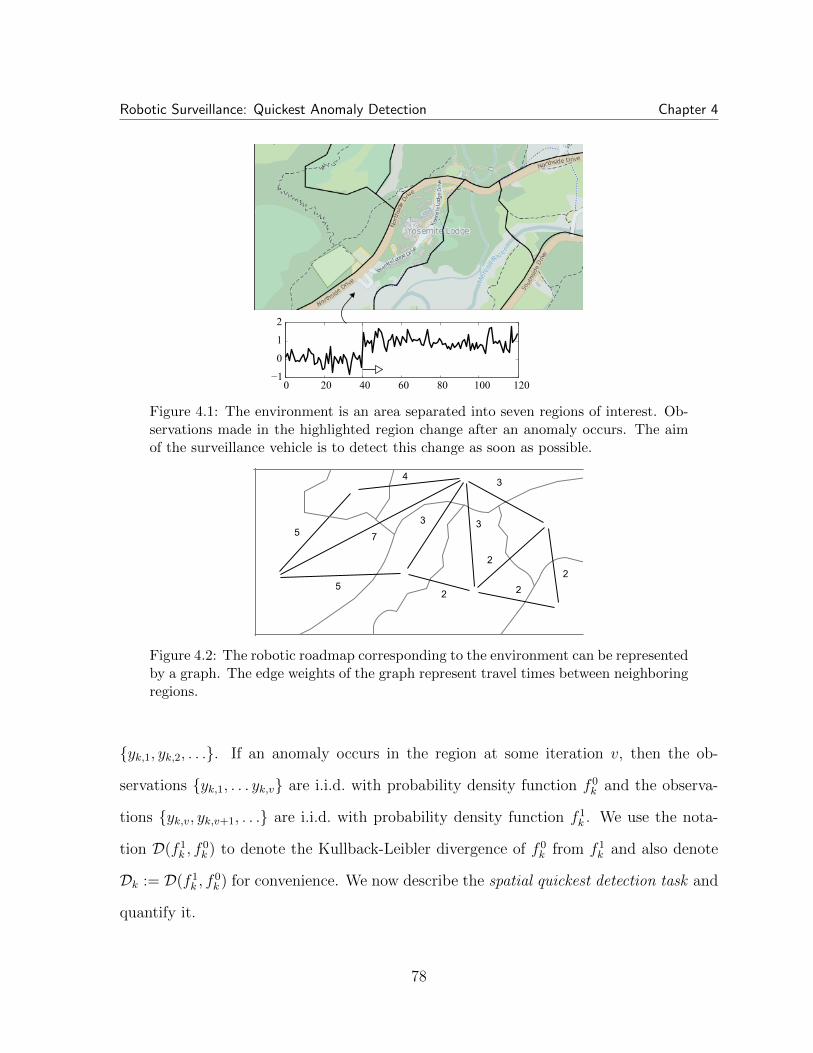
Robotic Surveillance: Quickest Anomaly Detection Chapter 4
0 20 40 60 80 100 120−1
0
1
2
anomaly
Figure 4.1: The environment is an area separated into seven regions of interest. Ob-servations made in the highlighted region change after an anomaly occurs. The aimof the surveillance vehicle is to detect this change as soon as possible.
2
22
3
2
3
4
5
5
73
Figure 4.2: The robotic roadmap corresponding to the environment can be representedby a graph. The edge weights of the graph represent travel times between neighboringregions.
{yk,1, yk,2, . . .}. If an anomaly occurs in the region at some iteration v, then the ob-
servations {yk,1, . . . yk,v} are i.i.d. with probability density function f 0
k and the observa-
tions {yk,v, yk,v+1
, . . .} are i.i.d. with probability density function f 1
k . We use the nota-
tion D(f 1
k , f0
k ) to denote the Kullback-Leibler divergence of f 0
k from f 1
k and also denote
Dk := D(f 1
k , f0
k ) for convenience. We now describe the spatial quickest detection task and
quantify it.
78

Robotic Surveillance: Quickest Anomaly Detection Chapter 4
4.3.3 Quickest Detection of Anomalies
The surveillance vehicle adopts a policy described by the tuple P = hP, qi. It moves
in the environment E = hV,E,D,wi according to a Markov chain with stationary distri-
bution q = [qi] 2 Rn⇥1 and transition matrix P = [pij] 2 Rn⇥n. If (i, j) 2 E, then pij � 0
and pij = 0 otherwise.
The aim of the vehicle is to detect anomalies in a region based on observations made
in that region in least amount of time possible. More specifically, using a routing policy
P , it is required to minimize the average detection delay defined below.
Definition 34 (Average Detection Delay) Let the vehicle service the environment
E = hV,E,D,wi using policy P for k 2 {1, . . . , n} and let �k(P) be the delay in detecting
an anomaly at region k. Then the task of the vehicle is to minimize the average detection
delay �avg(P) given by
�avg(P) =nX
k=1
wkE[�k(P)]. (4.1)
4.3.4 Ensemble CUSUM Algorithm
The surveillance vehicle visits the regions in E according to a realization of the Markov
chain with stationary distribution q and transition matrix P . When the vehicle is in a
particular region of the environment, it runs a local version of the CUSUM algorithm. We
refer to the n parallel CUSUM algorithms by Ensemble CUSUM Algorithm (Algorithm 4).
We wish to find the surveillance policy P = hP, qi for the environment E = hV,E,D,wi
which minimizes the average detection delay �avg
(P) defined in equation (4.1) in the
previous section.
Remark 35 (Service times): The service times required for conducting surveillance in
di↵erent regions are not modeled in the problem setup. However, they can be incorporated
79

Robotic Surveillance: Quickest Anomaly Detection Chapter 4
Algorithm 4: Ensemble CUSUM Algorithm
Given: Policy P = hP, qi, threshold ⌘, initial state x.Set: ⇤k,0 = 0 for k 2 {1, . . . , n}, local variable ⌧ = 1 for all regions.
1 Make observation yk,⌧ at region x. ;
2 ⇤x,⌧ =⇣
⇤x,⌧�1
+ log f1x
(yx,⌧
)
f0x
(yx,⌧
)
⌘
+
;
3 if ⇤x,⌧ > ⌘ then4 Declare an anomaly at region x.;5 Set ⇤x,⌧ = 0;6 end7 Set ⌧ ⌧ + 1 for x;8 Select x z with probability P (x, z) ;9 Repeat from step 1.
in a straighforward manner. If v 2 Rn⇥1 is the constant vector of service times, they can
be accounted for by modifying the travel time matrix to D := D + nvT .
Remark 36 (Knowledge of probability density functions): The probability density func-
tions in the absence and presence of anomalies are assumed to be known to the surveillance
vehicle. In a scenario where the probability density functions are not known, the CUSUM
algoithm can be replaced by the minimax robust quickest change detection algorithm [103]
and the results presented in this chapter can be extended to apply to that scenario as well.
4.4 Preliminary Results
We will now state some preliminary results which will be used in analysing the En-
semble CUSUM Algorithm. We will start by reviewing some performance guarantees on
the CUSUM algorithm.
80
Robotic Surveillance: Quickest Anomaly Detection Chapter 4
4.4.1 CUSUM Algorithm
The CUSUM algorithm is designed for quick prediction of anomalies while at the same
time, avoiding making false alarms [88]. In the CUSUM algorithm, at each iteration
⌧ 2 N made in region k, (i) observation yk,⌧ is collected, (ii) the statistic
⇤k,⌧ =
✓
⇤k,⌧�1
+ logf 1
k (yk,⌧ )
f 0
k (yk,⌧ )
◆
+
with ⇤k,0 = 0 is computed and (iii) a change is declared if ⇤k,⌧ > ⌘. Let Ok be the
observation at which an anomaly is declared at region k. For a given threshold ⌘, the
expectation of Ok conditioned on the presence of an anomaly, i.e. the worst expected
number of observations of the CUSUM algorithm is
Ef1k
(Ok) ⇡e�⌘ + ⌘ � 1
D(f 1
k , f0
k )=
⌘
Dk
, (4.2)
where ⌘ = e�⌘ + ⌘ � 1, and the expectation of Ok conditioned on the absence of an
anomaly, i.e. the false alarm rate for CUSUM algorithm is
Ef0k
(Ok) ⇡e⌘ � ⌘ � 1
D(f 0
k , f1
k )(4.3)
The approximations in equations (4.2,4.3) are referred to as the Walds approxima-
tions [88]. For large values of the threshold ⌘, these approximations are known to be
accurate. We also set
sk :=⌘
Dk
, (4.4)
and s = [sk] 2 Rn⇥1, referring to it as the vector of CUSUM samples. Given ⌘ and Dk,
the constant sk is the expected number of visits to region k required to detect an anomaly
81

Robotic Surveillance: Quickest Anomaly Detection Chapter 4
in that region.
The expression for the average detection delay of the Ensemble CUSUM Algorithm
(Algorithm 4) depends on the property of Markov chains called the first passage time
stated in Chapter 3.
4.5 Performance of the Ensemble CUSUM Algorithm
We are now ready to state our main results on the average detection delay �avg
(P) of
the Ensemble CUSUM Algorithm (Algorithm 4).
Theorem 37 (Performance of the Ensemble CUSUM Algorithm): For a single vehicle
conducting surveillance of the environment E = hV,E,D,wi according to the Ensemble
CUSUM Algorithm (Algorithm 4) using the policy P = hP, qi,
(i) the expected detection delay E[�k(P)] at region k satisfies
E[�k(P)] =nX
i=1
qinik + (sk � 1)nkk, (4.5)
(ii) the average detection delay �avg(P) over the entire environment satisfies
�avg(P) =nX
k=1
wk
nX
i=1
qinik + (sk � 1)nkk
!
, (4.6)
where N = [nij] 2 Rn⇥n is the first passage time matrix for the irreducible Markov chain
with transition matrix P 2 Rn⇥n and stationary distribution q 2 Rn⇥1 and the constant
s 2 Rn⇥1 is the vector of CUSUM samples.
Proof: Let ⌧ 2 {1, . . . , Ok} be the iterations at which the vehicle visits region
region k and sends information about it to the control center. Let Ok be the iteration at
82
Robotic Surveillance: Quickest Anomaly Detection Chapter 4
which an anomaly is detected in region k. The observation made at region k at the ⌧ -th
iteration in that region is denoted by yk,⌧ . Let the log likelihood ratio calculated by the
local CUSUM algorithm for that iteration be ✏k,⌧ . Then,
✏k,⌧ = logf 1
k (yk,⌧ )
f 0
k (yk,⌧ ).
Conditioned on the presence of an anomaly, {✏k,⌧}⌧k
2N are i.i.d. and Ef1k
[✏k,⌧ ] = Dk. Then,
referring to result summarized in equation (4.2), Ef1k
[Ok] = ⌘/Dk. Thus, the expected
time it takes for the Ensemble CUSUM Algorithm to make the Ok-th observation at
region k is essentially the expected detection delay �k(P) at region k. We will now
devote our attention to computing the expectation of �k(P).
Let t0k be the time at which the vehicle starts the CUSUM algorithm. Let {t1k, t2k, . . . tO
k
k }
be the time instant at which it leaves region k, having serviced it, and �tik = ti+1
k � tik for
i = {0, 1, 2, . . .}. Then, the detection delay �k(P ) = tOk
k =PO
k
i=0
�tik. The expectation of
�k(P ) can be computed:
E[�k(P )] =E"
Ok
�1
X
i=0
�tik
#
= E[�t0k] + E"
Ok
�1
X
i=1
�tik
#
,
=E[�t0k] + (E[Ok]� 1)E[�tik] (4.7)
=nX
i=1
qinik +
✓
⌘
Dk
� 1
◆
nkk. (4.8)
Equation (4.7) comes from the application of Wald’s identity. Notice that E[�t0k] is the
expected time to start from any node and visit node k for the first time and given i > 0,
E[�tik] is the expected time taken to return to node k. Recollect that nij is the expected
time for the vehicle to start from node i to visits node j for the first time. Hence, we can
conclude that E[�t0k] =Pn
i=1
qinik and E[�tik] = nkk for i > 0 to obtain equation (4.8).
83
Robotic Surveillance: Quickest Anomaly Detection Chapter 4
Using the definition of s from equation (4.4), the first result follows. Next, using the
definition of �avg
(P) from equation (4.1), the second result follows.
Thus, the average detection delay depends on the first passage times between nodes
of the graph representing the environment E . We now present a modified expression for
�avg
(P), removing the dependence of the first passage times, in the following theorem.
The proof of the theorem is postponed to Appendix.
Theorem 38 (Average detection delay): For a single vehicle conducting surveillance of
the environment E = hV,E,D,wi according to the Ensemble CUSUM Algorithm (Algo-
rithm 4) using the policy P = hP, qi,
�avg(P) = � Tn [(((I � P ) + (P �D) nq
T ))�1 � I](r · w) + (� � 1) + �(s� n)T (r · w),
(4.9)
where r 2 Rn⇥1 with r · q = n, I 2 Rn⇥n is the identity matrix, � = qT (P � D) n and
the constant s 2 Rn⇥1 is the vector of CUSUM samples.
In our setup, the environment can have an arbitrary graph topology and the routing
policy can also take an arbitrary form adhering to the restrictions imposed by the graph
topology. A specific simplification, where the environment is an all to all graph and
where the transition matrix for the routing policy has the form P = nqT is explored in
[95]. While they provide algorithms to optimize the transition matrix q in the simplified
setup, we consider the more generalized problem. Specifically, our goal is to find policy
P = hP, qi for the vehicle such that �avg
(P) is minimized. This can be framed as the
following optimization problem:
Problem 6 ( Minimizing the average detection delay): Given the environment
E = hV,E,D,wi and the constant vector of CUSUM samples s 2 Rn⇥1, determine the
84
Robotic Surveillance: Quickest Anomaly Detection Chapter 4
stationary distribution q = [qi] 2 Rn⇥1 and transition probabilities P = [pij] 2 Rn⇥n
solving:
minimize � Tn [(((I � P ) + (P �D) nq
T ))�1 � I](r · w)
+ (� � 1) + �(s� n)T (r · w)
subject to P n = n, for each i 2 {1, . . . , n}
0 pij 1, for each (i, j) 2 E
pij = 0, for each (i, j) /2 E
qTP = qT , for each (i, j) 2 E
qT n = 1, qi � 0, for each i 2 {1, . . . , n}
P irreducible,
� = qT (P �D) n, r · q = n.
The above optimization problem contains the constraint that the transition matrix
be irreducible. Since it is hard to enforce the irreducibility constraint during each step of
an iterative optimization algorithm, our approach is to relax the irreducibility constraint
and verify that the final solution satisfies the constraint. A Markov chain that is not irre-
ducible contains multiple communicating classes, making the first passage time between
at least one pair of regions infinite. Since the average detection delay depends on the
first passage times of the chain, the outcome where the final solution is a reducible chain
would drive up the cost function of the optimization problem, making such an outcome
highly unlikely. Because of this reason, the relaxation of the irreducibility constraint
works very well in practice.
Let P⇤ be the solution to Problem 6 and let �⇤avg
:= �avg
(P⇤). The cost function
of this optimization problem is not a convex function of P and q. Moreover, one of
85
Robotic Surveillance: Quickest Anomaly Detection Chapter 4
the constraints is also nonlinear. We now devote some attention to determining an
upper bound on �⇤avg
, and frame an optimization problem to minimize it. We start with
evaluating policies of the form Pw = hPw, wi, i.e., where the Markov chain corresponding
to the policy has the stationary distribution w. We leverage the result known on the
weighted sum of the first passage times from Theorem 25 to simplify expressions for the
detection delay of the Ensemble CUSUM algorithm in this case.
Theorem 39 (Upper bound on average detection delay): For a single vehicle conducting
surveillance of the environment E = hV,E,D,wi according to the Ensemble CUSUM
Algorithm (Algorithm 4) using the policy Pw = hPw, wi,
�avg(Pw) =�
wT (Pw �D) n
�
nX
i=2
1
1� �i(Pw)+ (s� n)
Tn
!
for all Pw 2 Sw, where Sw is the set of transition matrices corresponding to irreducible
Markov chains with stationary distribution w, {�1
(Pw), . . . ,�n(Pw)} are the eigenvalues
of Pw with �1
(Pw) = 1, and the constant s 2 Rn⇥1 is the vector of CUSUM samples.
Proof: We start with the expression for �avg
(P) obtained in Theorem 37. In matrix
form, equation (4.6) can be rewritten as
�avg
(P) = qTNw + (s� n)TNdw, (4.10)
where P = hP, qi. Setting the variable q to w, and using the result from Theorem 25, as
well as the result from Theorem. 23 (ii), equation (4.10) can be simplified:
�avg
(Pw) =wTNw + (s� n)TNdw,
=�
wT (Pw �D) n
�
nX
i=2
1
1� �i(Pw)+ (s� n)
Tn
!
,
86

Robotic Surveillance: Quickest Anomaly Detection Chapter 4
We can make the upper bound obtained on the optimal detection delay tighter by
choosing Pub
2 Sw which minimizes the average detection delay. The following optimiza-
tion problem can be framed to find the matrix Pub
.
Problem 7 (Minimizing the upper bound on optimal average detection delay): Given
the environment E = hV,E,D,wi, the vector of CUSUM samples s 2 Rn⇥1 and the
stationary distribution w 2 Rn⇥1, determine the transition probabilities P = [pij] 2 Rn⇥n
solving:
minimize�
wT (P �D) n
�
nX
i=2
1
1� �i(P )+ (s� n)
Tn
!
subject to P n = n, for each i 2 {1, . . . , n}
0 pij 1, for each (i, j) 2 E
pij = 0, for each (i, j) /2 E
wipij = wjpji, for each (i, j) 2 E.
(4.11)
Note that the above optimization problem also involves the restriction of non-reversibility
on the transition matrix P as denoted by the last equality.
Theorem 40 (Convexity of Optimization Problem 7): Let Sw be the set of transition
matrices associated with irreducible non-reversible Markov chains on graph G = (V,E)
and having the stationary distribution w. Then, the Optimization Problem 7 is convex.
Proof: From Theorem 39, the cost function f(Pw) of the Optimization Problem 7
can be written down as:
f(Pw) =�
wT (Pw �D) n
�
nX
i=2
1
1� �i(Pw)
!
+�
wT (Pw �D) n
�
(s� n)T
n. (4.12)
87

Robotic Surveillance: Quickest Anomaly Detection Chapter 4
The first term in equation (4.12) is the mean first passage time of the Markov chain as
defined in Theorem 25. The mean first passage time is a convex function over the set Sw
(refer to [78] for the proof). Moreoever, the second term in equation (4.12) is an a�ne
function over the set Sw. Since the positive weighted sum of convex and a�ne functions
is convex, the function Pw 7! f(Pw) is convex over the set Sw. The set Sw is also convex
and the constraints of the problem are a�ne. Hence, the optimization problem is convex.
The Optimization Problem 7 can be written as a semidefinite program. In order to do
this, the expression for the detection delay is rewritten in terms of the trace of a matrix:
�avg
(Pw) =�
wT (Pw �D) n
�
nX
i=2
1
1� �i(Pw)+ (s� n)
Tn
!
,
=�
wT (Pw �D) n
�
Tr⇥
(I �W 1/2PwW�1/2 + wcw
Tc )
�1
⇤
+�
wT (Pw �D) n
�
(s� n)T
n,
where W = diag[w] and the column vector wc = (pw
1
, . . . ,pwn)T . The first equation
comes from Theorem 39 and the first part of the second equation is because of a relation
between the trace of a function of Pw and its eigenvalues [78]. Using this form for �avg
(Pw),
we can now formulate an SDP as shown below.
Problem 8 (Minimizing the upper bound on the optimal average detection delay (SDP)):
Given the environment E = hV,E,D,wi and vector of CUSUM samples s 2 Rn⇥1, with
W = diag[w] and wc = (pw
1
, . . . ,pwn)T , determine Y = [yij] 2 Rn⇥n, X 2 Rn⇥n, t 2 R
88
Robotic Surveillance: Quickest Anomaly Detection Chapter 4
and u 2 R solving:
minimize Tr[X] + u(sT n)
subject to2
6
4
t(I + wcwTc )�W 1/2YW�1/2 I
I X
3
7
5
> 0
2
6
4
t 1
1 u
3
7
5
> 0
nX
j=1
yij = t, for each i 2 {1, . . . , n}
wiyij = wjyji, for each (i, j) 2 E
0 yij t, for each (i, j) 2 E
yij = 0, for each (i, j) /2 E
wT (Y �W ) n = 1
t � 0.
Then, the transition matrix Pw is given by Pw = Y/t.
Let Pub
be the solution to the Optimization Problem 7. We refer to the policy
Pub
= hPub
, wi as the e�cient policy for convenience.
4.6 Numerical Simulations
We now study the spatial quickest detection task for a specific environment. In
particular, we are interested in examining the e�ciency of the upper bound service policy
Pub
= hPub
, wi compared to the optimal policy P⇤ which minimizes the average detection
89

Robotic Surveillance: Quickest Anomaly Detection Chapter 4
1 2 3 4 5 6 7 8 9 10
0
500
1000
1500
�
⇥ avg
optimal policy
efficient policy
fastest mixing chain
policy from [18]
Monte Carlo simulations
for optimal policy
Figure 4.3: Variation of the average detection delay using the optimal policy �
⇤avg
(black squares), the e�cient policy �
ub
(grey squares), the policy based on the fastestmixing non-reversible Markov chain with a uniform stationary distribution (grey cir-cles) and the policy in [95] (black circles) with respect to the threshold ⌘ of theCUSUM algorithm. Expected detection delay for the optimal policy using MonteCarlo Simulations (dashed lines).
2 4 6 8 100
200
400
600
800
1000
�
⇥ avg
optimal policyefficient policyfastest mixing chainpolicy from [18]
Figure 4.4: Average detection delay using the optimal policy �
⇤avg
(black squares) andthe e�cient policy �
ub
(grey squares) are compared with the average detection delayobtained using the policy based on the fastest mixing non-reversible Markov chain(grey circles) with a uniform stationary distribution and the policy from [95] (blackcircles) for various levels on noise in observations made in the second region.
delay. We also compare these two policies to some candidate policies (namely the policy
based on the fastest mixing non-reversible Markov chain [18] and a policy proposed in
[95]).
Environment and modeling of anomalies: The environment (Fig. 4.1) is an
90
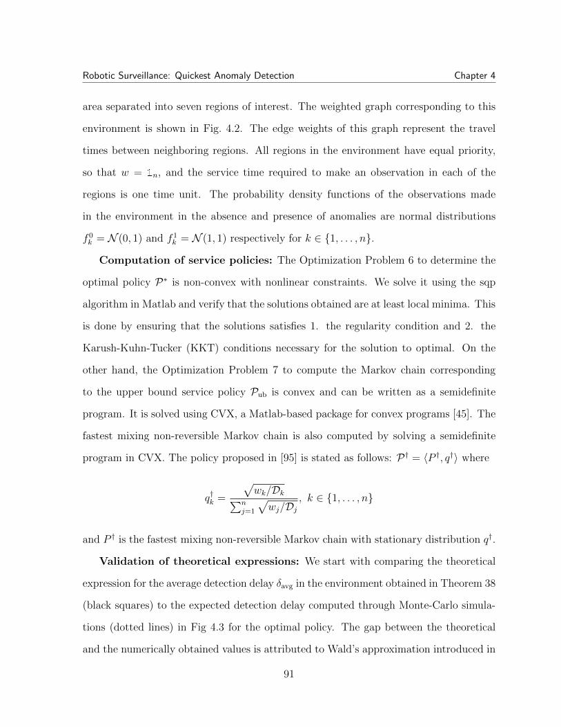
Robotic Surveillance: Quickest Anomaly Detection Chapter 4
area separated into seven regions of interest. The weighted graph corresponding to this
environment is shown in Fig. 4.2. The edge weights of this graph represent the travel
times between neighboring regions. All regions in the environment have equal priority,
so that w = n, and the service time required to make an observation in each of the
regions is one time unit. The probability density functions of the observations made
in the environment in the absence and presence of anomalies are normal distributions
f 0
k = N (0, 1) and f 1
k = N (1, 1) respectively for k 2 {1, . . . , n}.
Computation of service policies: The Optimization Problem 6 to determine the
optimal policy P⇤ is non-convex with nonlinear constraints. We solve it using the sqp
algorithm in Matlab and verify that the solutions obtained are at least local minima. This
is done by ensuring that the solutions satisfies 1. the regularity condition and 2. the
Karush-Kuhn-Tucker (KKT) conditions necessary for the solution to optimal. On the
other hand, the Optimization Problem 7 to compute the Markov chain corresponding
to the upper bound service policy Pub
is convex and can be written as a semidefinite
program. It is solved using CVX, a Matlab-based package for convex programs [45]. The
fastest mixing non-reversible Markov chain is also computed by solving a semidefinite
program in CVX. The policy proposed in [95] is stated as follows: P† = hP †, q†i where
q†k =
p
wk/DkPn
j=1
p
wj/Dj
, k 2 {1, . . . , n}
and P † is the fastest mixing non-reversible Markov chain with stationary distribution q†.
Validation of theoretical expressions: We start with comparing the theoretical
expression for the average detection delay �avg
in the environment obtained in Theorem 38
(black squares) to the expected detection delay computed through Monte-Carlo simula-
tions (dotted lines) in Fig 4.3 for the optimal policy. The gap between the theoretical
and the numerically obtained values is attributed to Wald’s approximation introduced in
91

Robotic Surveillance: Quickest Anomaly Detection Chapter 4
equation (4.2).
Comparison of performances of service policies: We first compare variation
in the performance of various service policies with respect to di↵erent thresholds ⌘ of
the CUSUM algorithm in Fig. 4.3(a). The average detection delay �ub
obtained using
the e�cient policy Pub
(grey squares) is close to the optimal average detection delay
�⇤avg
(black squares) for lower values of the threshold ⌘. The gap observed between the
optimal solution and the upper bound can be attributed to two factors: freedom to
choose any stationary distribution as well as relaxation of the nonreversibility constraint
for computing the optimal solution. In comparison, the performance of the fastest mixing
non-reversible Markov chain with stationary distribution w = n (grey circles) and the
policy proposed in Theorem 6 in [95] (black circles) is much poorer. This is expected
since the e�cient policy is guaranteed to perform better in comparison to the fastest
mixing non-reversible Markov chain with the same stationary distribution.
Next, we study the e↵ect of the variation in the probability density functions of
observations on the performance of the service policies. We consider a scenario where
the second region, which is a residential area in our illustration, is a↵ected by noisy
observations. While the probability distribution functions for observations in all the
other regions remain same, they are di↵erent for the second region: f 0
2
= N (0, �) and
f 1
2
= N (1, �). The average detection delays for the various policies considered in the
chapter are compared for di↵erent values of � in Fig. 4.4. The performance of the
e�cient policy (grey squares) is very close to the optimal performance (black squares)
for a wide range of � in this case. In comparison, the performances of the policy based on
the fastest mixing non-reversible chain with stationary distribution w = n (grey circles)
and the policy from [95] (black circles) are much poorer. They also get worse for noisier
observations.
92

Robotic Surveillance: Quickest Anomaly Detection Chapter 4
Appendix
Proof of Theorem 38: We start from the expression for �avg
(P) obtained in Theorem 37.
Using the definition of s stated in the statement of the theorem, and equation (4.6), the
expression for �avg
(P) can be written in matrix form as follows:
�avg
(P) = qTNw + (s� n)TNdw. (4.13)
We first work towards simplifying the first term in equation (4.13). The first passage
time matrix satisfies equation (3.6). Using this and the identity from Lemma 33, and the
assumption that Tnw = 1, the term qTNw can be simplified:
qTNw =qT�( nTnGd + I �G)Q�1w,= �( T
nGd + qT (I �G))Q�1w,
=�( TnGd + qT � qT
�)Q�1w = � T
nGdQ�1w + (� � 1)qTQ�1w,
=� TnGdQ
�1w + (� � 1) Tnw = � T
nGdQ�1w + (� � 1). (4.14)
where Q = diag[q]. Looking at the first term in equation (4.14),
TnGdQ
�1w = Tn [(((I � P ) + (P �D) nq
T ))�1 �Q�1]w,
= Tn [(((I � P ) + (P �D) nq
T ))�1 � I](r · w).
Substituting Ndw = �Q�1w = �(r � w) from equation (3.8) into the second term in
equation (4.13), the result follows.
93

Chapter 5
Synchronization of Beads on a Ring
We now consider the problem of synchronization of n robotic agents that control their
motion on a ring and that communicate when in close proximity of each other. One
application of this setup is as a boundary-patrolling algorithm which has numerous ap-
plications, e.g. in monitoring of spreading fires, toxic-area containment and clean-up, and
the sensing of sharp temperature gradient surfaces in the sea. These algorithms require
sporadic communication among agents, which have to optimally divide the task among
themselves without the intervention of a supervisor.
We therefore pose the question: can n intelligent agents (or beads), capable of control-
ling their motion, autonomously organize themselves so that each one sweeps a sector of
the ring and impacts with the neighboring beads always at the boundaries of the sector?
In other words, can they reach a periodic orbit and get in sync?
Apart from boundary-guarding the problem is also of general interest: If the n agents
control their motion to simulate n beads sliding on a frictionless hoop, then we know
that their dynamics is very rich. In fact, in [30], the authors study extensively the case
of n = 3 and prove the existence of periodic as well as chaotic orbits.
94

Synchronization of Beads on a Ring Chapter 5
5.1 Contributions
We state the contributions of this chapter 1 now. We design a distributed algorithm
that allows a collection of beads to reach synchronization and that is robust to failure of
beads. The algorithm requires the beads to slowdown and speedup immediately prior to
and after impact respectively; accordingly, we refer to the algorithm as the “slowdown,
impact and speedup algorithm.” The beads can be deployed with arbitrary initial posi-
tions and speeds. At the desired steady state, every bead sweeps a sector of equal length,
and neighboring beads meet always at the same point. If n is even, the beads all travel
at the same speed, while if n is odd, the beads travel at the same average speed. Two
beads exchange information only when they impact. We provide a su�cient condition on
the initial positions of the beads to guarantee converegence of beads. Extensive simula-
tions show that synchronization is reached in general, even when the assumptions are not
satisfied. Moreover, our algorithm confers certain robustness properties on the emerging
synchronized behavior, which is of interest for any control system.
5.2 Organization
This chapter is organized as follows. Section 5.1 states the contributions of the
work. We then introduce the notation employed and describe in detail what is meant by
agent or bead synchronization on a circular boundary in Section 5.3. The discrete-time
synchronization algorithm is presented in Section 5.4. A set of preliminary results on
which the main theorems build upon is presented in 5.5. The main results that allow us
to analyze the algorithm are included in 5.6. Finally, we present simulations in Section 5.7
showing that convergence of the algorithm is indeed possible in most general cases.
1This work is in collaboration with Dr. Sara Susca and Prof. Sonia Martınez
95
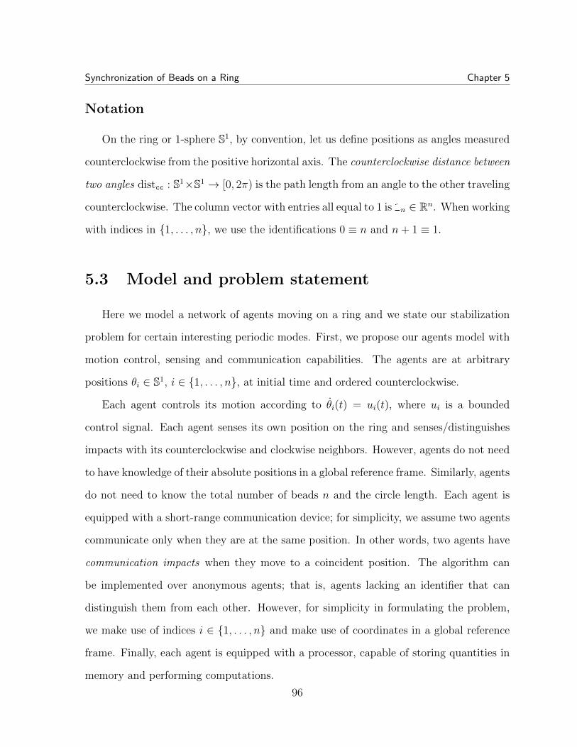
Synchronization of Beads on a Ring Chapter 5
Notation
On the ring or 1-sphere S1, by convention, let us define positions as angles measured
counterclockwise from the positive horizontal axis. The counterclockwise distance between
two angles distcc : S1⇥S1 ! [0, 2⇡) is the path length from an angle to the other traveling
counterclockwise. The column vector with entries all equal to 1 is n 2 Rn. When working
with indices in {1, . . . , n}, we use the identifications 0 ⌘ n and n+ 1 ⌘ 1.
5.3 Model and problem statement
Here we model a network of agents moving on a ring and we state our stabilization
problem for certain interesting periodic modes. First, we propose our agents model with
motion control, sensing and communication capabilities. The agents are at arbitrary
positions ✓i 2 S1, i 2 {1, . . . , n}, at initial time and ordered counterclockwise.
Each agent controls its motion according to ✓i(t) = ui(t), where ui is a bounded
control signal. Each agent senses its own position on the ring and senses/distinguishes
impacts with its counterclockwise and clockwise neighbors. However, agents do not need
to have knowledge of their absolute positions in a global reference frame. Similarly, agents
do not need to know the total number of beads n and the circle length. Each agent is
equipped with a short-range communication device; for simplicity, we assume two agents
communicate only when they are at the same position. In other words, two agents have
communication impacts when they move to a coincident position. The algorithm can
be implemented over anonymous agents; that is, agents lacking an identifier that can
distinguish them from each other. However, for simplicity in formulating the problem,
we make use of indices i 2 {1, . . . , n} and make use of coordinates in a global reference
frame. Finally, each agent is equipped with a processor, capable of storing quantities in
memory and performing computations.
96

Synchronization of Beads on a Ring Chapter 5
Figure 5.1: The figure shows a collection of four beads moving in balanced synchronization.
Next, we describe some interesting periodic trajectories for n beads moving on a ring.
It is our objective, in the following sections, to design a motion control and communica-
tion algorithm to render such trajectories attractive.
Definition 41 (Balanced synchronization) Consider a collection of n beads moving
on a ring. The collection of beads is balanced synchronized with period T , if (i) any
two neighboring beads impact always at the same point, (ii) the time interval between
two consecutive impacts, involving the same beads, has duration T , and (iii) all the beads
impact simultaneously. In other words, in a balanced synchronized collection, each bead
sweeps an arc of length 2⇡/n at constant speed 2 2⇡nT
.
An example of a collection of four beads in sync is shown in Figure 5.1: each bead
sweeps an arc at the boundaries of which it impacts with one of its neighbors and the
impacts happen simultaneously.
If n is odd, then balanced synchronization cannot be reached. Therefore, we give the
following weaker synchronization notion, reachable also for odd n.
Definition 42 (Unbalanced synchronization) Consider a collection of n beads mov-
ing on a ring. The collection of beads is unbalanced synchronized with period T , if (i)
97
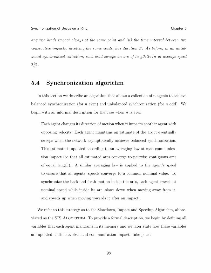
Synchronization of Beads on a Ring Chapter 5
any two beads impact always at the same point and (ii) the time interval between two
consecutive impacts, involving the same beads, has duration T . As before, in an unbal-
anced synchronized collection, each bead sweeps an arc of length 2⇡/n at average speed
2 2⇡nT
.
5.4 Synchronization algorithm
In this section we describe an algorithm that allows a collection of n agents to achieve
balanced synchronization (for n even) and unbalanced synchronization (for n odd). We
begin with an informal description for the case when n is even:
Each agent changes its direction of motion when it impacts another agent with
opposing velocity. Each agent maintains an estimate of the arc it eventually
sweeps when the network asymptotically achieves balanced synchronization.
This estimate is updated according to an averaging law at each communica-
tion impact (so that all estimated arcs converge to pairwise contiguous arcs
of equal length). A similar averaging law is applied to the agent’s speed
to ensure that all agents’ speeds converge to a common nominal value. To
synchronize the back-and-forth motion inside the arcs, each agent travels at
nominal speed while inside its arc, slows down when moving away from it,
and speeds up when moving towards it after an impact.
We refer to this strategy as to the Slowdown, Impact and Speedup Algorithm, abbre-
viated as the SIS Algorithm. To provide a formal description, we begin by defining all
variables that each agent maintains in its memory and we later state how these variables
are updated as time evolves and communication impacts take place.
98
Synchronization of Beads on a Ring Chapter 5
Algorithm Variables
Each agent i 2 {1, . . . , n} maintains in memory the following tuple:
vi 2 R>0
, the nominal speed,
di 2 {�1,+1}, the direction of motion,
ai 2 {�1,+1}, the moving-away flag,
`i 2 S1, the arc lower boundary, and
ui 2 S1, the arc upper boundary.
Regarding initialization, we allow vi(0), di(0) to be arbitrary and we set `i(0) = ui(0) :=
✓i(0), and ai(0) := di(0).
Given these definitions, it is convenient to introduce the following notation and
nomenclature. First, we define the ith processor state xi := (vi, di, ai, `i, ui) and call
(✓i, xi) the ith agent state. Next, we associate an arc of the ring to each bead. This arc
is the fraction of the ring that each bead eventually sweeps when balanced synchrony
(as in Definition (41)) is asymptotically reached. To each bead i, we associate a desired
sweeping arc defined by
Arc(`i, ui) = {✓ 2 S1 | distcc(`i, ✓) distcc(`i, ui)}.
This quantity will also be denoted by Di for convenience henceforth.
Algorithm Rules
The algorithm rules specify how the agents move in continuous time and how they
update their processor states when certain events happen.
99

Synchronization of Beads on a Ring Chapter 5
First, at all time t � 0, each bead sets its velocity ✓i depending on whether the bead
is traveling inside its desired sweeping arc, or, if outside the sweeping arc, depending
on whether it is moving away from or towards the sweeping arc. Specifically, given two
scalar gains 1
2
< f < 1 and h = f2f�1
> 1, we set
✓i(t) := di(t)vi(t) ·
8
>
>
>
>
>
>
<
>
>
>
>
>
>
:
1, if ✓i(t) 2 Di,
f, if ✓i(t) /2 Di and di(t) = ai(t),
h, if ✓i(t) /2 Di and di(t) = �ai(t).
Second, the ith processor state changes only when one of the following two events
occurs: an Impact Event which takes place with either bead i� 1 or with bead i+ 1, or
a Crossing Event which takes place when bead i crosses either `i or ui while leaving its
desired sweeping arc.
(Impact Event) If at time t an impact occurs for bead i with either bead i+1 or i�1,
then: (1) the two beads exchange through communication their processors states, and
(2) with this information, each bead updates its memory as follows. We define an impact
between beads i and i+1 to be of head-to-tail type if di(t) = di+1
(t), and of head-to-head
100

Synchronization of Beads on a Ring Chapter 5
type if instead di(t) = �di+1
(t). The ith processor state is updated according to:
vi(t+) :=
8
>
>
<
>
>
:
1
2
�
vi(t) + vi�1
(t)�
, if the impact occurs with i� 1,
1
2
�
vi(t) + vi+1
(t)�
, if the impact occurs with i+ 1,
(5.1)
di(t+) :=
8
>
>
<
>
>
:
�di(t), if the impact is head-to-head type,
di(t), otherwise,
(5.2)
ai(t+) := ai(t),
`i(t+) :=
8
>
>
<
>
>
:
Ci(t)� 1
2
distcc(Ci�1
(t), Ci(t)), if the impact occurs with i� 1,
`i(t), if the impact occurs with i+ 1,
(5.3)
ui(t+) :=
8
>
>
<
>
>
:
ui(t), if the impact occurs with i� 1,
Ci(t) +1
2
distcc(Ci(t), Ci+1
(t)), if the impact occurs with i+ 1,
(5.4)
where the upper-script + indicates the variable value right after the impact, and where
we define the center Ci 2 S1 of the desired sweeping arc Di by Ci = `i + distcc(`i, ui)/2.
Note that, after an impact between beads i and i � 1, we have `i�1
(t+) = ui(t+)
because they both are defined as the midpoint of the arc from Ci�1
(t) to Ci(t).
(Crossing Event) The memory of each bead i is updated also when the agent crosses
either `i(t) or ui(t) while leaving its desired sweeping arc. The nominal speed vi, the
direction di and the boundary of the sweeping arc `i and ui do not change,
vi(t+) := vi(t), di(t
+) := di(t), `i(t+) := `i(t), ui(t
+) := ui(t),
The flag ai is updated as follows:
ai(t+) := di(t).
101

Synchronization of Beads on a Ring Chapter 5
Here the upper-script + indicates the value of the memory right after bead i crosses the
boundary of its desired sweeping arc.
Only two-way impacts have been considered in the above algorithm. However, im-
pacts between three or more beads can be assumed to be a sequence of two-way impacts
separated by infinitesimal times. By default, impacts between beads with smaller in-
dices can be addressed first. Although the order in which they are addressed a↵ects the
subsequent motion of the beads, it does not a↵ect the convergence results of the SIS
Algorithm.
5.5 Preliminary results
In this section we prove some preliminary results before we can prove the correctness
of the SIS Algorithm. We begin with an important characterization of initial states.
Definition 43 (Admissible balanced and unbalanced configurations) A state
{(✓i, xi)}i2{1,...,n} is
(1) directionally balanced ifPn
i=1
di = 0
(2) directionally D-unbalanced for D 2 {�n+ 1, . . . , n� 1} \ {0}, ifPn
i=1
di = D.
Furthermore, a state has an admissible configuration if in addition to being directionally
balanced or D-unbalanced, for all i, j 2 {1, . . . , n} and j 6= i, ✓i 6= ✓j. The set of admis-
sible balanced configurations, and admissible D-unbalanced configurations are denoted
by A0�bal
, and AD�unbal
respectively.
Note that {(✓i, xi)}i2{1,...,n} 2 A0�bal
if and only if n is even and n/2 beads are moving
clockwise and n/2 are moving counterclockwise.
102

Synchronization of Beads on a Ring Chapter 5
Next, at each time t � 0, we define the impact graph G(t) as the undirected graph
with vertex set {1, . . . , n} and with edge set defined by the following rule: the pair (i, j)
is an edge in G(t) if the beads i and j collide at time t.
Proposition 1 (Uniform connectivity of impact graphs) Along the trajectories of
the SIS Algorithm, with {(✓i(0), xi(0))}i2{1,...,n} 2 A0�bal
S
AD�unbal
, for all t0
� 0 the
graphS
t2[t0,t0+2⇡/(fvmin)]G(t) is connected.
The proof of Proposition 1 builds up on the following facts.
Lemma 44 (Properties) Along the trajectories of the SIS Algorithm, with
{(✓i(0), xi(0))}i2{1,...,n} 2 A0�bal
S
AD�unbal
:
(1)Pn
i=1
di(t) is constant,
(2) any two desired sweeping arcs are disjoint or share at most a boundary point, fur-
thermore their label index increases in the counterclockwise direction, i.e., ui(t) =
`i+1
(t),
(3) the order of the beads is preserved, i.e., for all i, j 2 {1, . . . , n}, j 62 {i, i+ 1}, and
t � 0, we have distcc(✓i(t), ✓i+1
(t)) distcc(✓i(t), ✓j(t)). Therefore, a bead i can
impact only its immediate neighbors i� 1 and i+ 1.
Proof: See Appendix
Lemma 45 (Impacts in bounded interval) Let vmin
= mini2{1,...,n} vi(0). Along the
trajectories of the SIS Algorithm, with {(✓i(0), xi(0))}i2{1,...,n} 2 A0�bal
S
AD�unbal
,
for all i 2 {1, . . . , n} and for all t0
> 0, bead i impacts at least once with both its
neighbors i� 1 and i+ 1 across the interval [t0
, t0
+ 2⇡fvmin
].
Proof: See Appendix
103

Synchronization of Beads on a Ring Chapter 5
Figure 5.2: This figure shows that, regardless from where and with which velocitiesbeads i and i + 1 impact, the order of the beads is preserved. The velocities in thefigure are the velocities after the impact. The speed v is just the average value of vi
and vi+1
before the impact.
104

Synchronization of Beads on a Ring Chapter 5
Proof: [of Proposition 1] Because of Lemma 45, for all i and for all t0
there exist
t1
and t2
2 [t0
, t0
+ 2⇡fvmin
] such that G(t1
) and G(t2
) have respectively an edge between
vertices i and i+1 and between vertices i and i�1. Therefore, the graphS
t2[t0,t0+ 2⇡fv(0) ]
G(t)
contains the ring graph.
5.6 Convergence analysis
In the first part of this section we prove that the nominal speeds vi of all the beads
will asymptotically be equal to the average of their initial values, and that the desired
sweeping arc will asymptotically attain a length 2⇡/N . In the second and third part of
this section we show that SIS Algorithm enables the beads to reach balanced synchrony
if n is even and unbalanced synchrony if n is odd. We begin our convergence analysis
with a useful result that combines known facts from [40, 102, 72]. Given a symmetric
stochastic matrix F 2 RN⇥N , its associated graph has node set {1, . . . , N} and edge set
defined as follows: (i, j) is an edge if and only if Fij > 0.
Theorem 46 (Average Consensus Dynamics) Consider a sequence of symmetric
stochastic matrices {F (`) | ` 2 Z�0
} ⇢ RN⇥N and the dynamical system
x(`+ 1) = F (`)x(`).
Let G(`) be the graph associated with F (`). Assume that
(A1) G(`) has a self loop at each node,
(A2) Each non-zero edge weight Fij(`), including the self-loops weights Fii(`), is larger
than a constant ↵ > 0, and
(A3) The graph [⌧�`G(⌧) is connected for all ` 2 Z�0
.
105
Synchronization of Beads on a Ring Chapter 5
Then the system is said to achieve average consensus with
lim`!+1
x(`) =⇣ 1
N
NX
i=1
xi(0)⌘
N .
We also define some terminology associated with movement of the beads on the
ring. Let the kth impact between beads i and i + 1 occur at the instant Iki . Let Ik =
[Ik1
, . . . , Ikn]T 2 Rn. Let us also define the kth passage time P k
i as the instant at which
bead i passes by the center of its desired sweeping arc after its kth but before its (k+1)th
impact. Let P k = [P k1
, . . . , P kn ]
T 2 Rn.
5.6.1 Convergence of nominal speed and desired sweeping arc
We start by proving that all nominal speeds vi converge to being equal to the average
of their initial values.
Lemma 47 (Speed convergence) Let v(t) = [v1
(t), . . . , vn(t)]T 2 Rn. Along the tra-
jectories of the SIS Algorithm, with {(✓i(0), xi(0))}i2{1,...,n} 2 A0�bal
S
AD�unbal
:
limt!+1
v(t) =Tnv(0)
nn.
Proof: For all i 2 {1, . . . , n}, define Ai 2 Rn⇥n by:
[Ai]lm =
8
>
>
>
>
>
>
<
>
>
>
>
>
>
:
1
2
, if (l,m) 2 {(i, i), (i, i+ 1), (i+ 1, i), (i+ 1, i+ 1)},
1, if l = m and l 62 {i, i+ 1},
0, otherwise .
106

Synchronization of Beads on a Ring Chapter 5
Because of equation (5.1),
v(Iki + ") = Aiv(Iki ).
where Iki + " is the time instant just after the impact. This can be extended to account
for more than one two-way impacts taking place at the same instant. For example, if
two separate impacts occur between beads i and i+ 1 as well as j and j + 1 at Iki , then
v(Iki + ") = AiAjv(Iki ).
Therefore, the dynamics of v(t) is the average consensus dynamics with matrices Ai.
Proposition 1 ensures that the sequence of impact graphs at impact instants is uniformly
jointly connected. Therefore, the assumptions of Theorem 46 are satisfied and we know
that all velocities vi(t) converge to 1
n
Pni=1
vi(0).
We now prove that the desired sweeping arcs converge asymptotically to a stationary
configuration in which all sweeping arcs have length 2⇡/n.
Lemma 48 (Convergence of desired sweeping arc) Let Li(t) = distcc(`i(t), ui(t))
be the length of the desired sweeping arc Di for i 2 {1, . . . , n}, and L(t) = [L1
(t), . . . , Ln(t)]T
2 Rn. Along the trajectories of the SIS Algorithm, with {(✓i(0), xi(0))}i2{1,...,n} 2
A0�bal
S
AD�unbal
, the arc lengths and the arcs converge, that is,
limt!+1
L(t) =2⇡
nn,
and the limits limt!+1 `i(t) and limt!+1 ui(t) exist and are finite.
107

Synchronization of Beads on a Ring Chapter 5
Proof: For all i 2 {1, . . . , n}, define Bi 2 Rn⇥n by:
[Bi]lm =
8
>
>
>
>
>
>
>
>
>
>
<
>
>
>
>
>
>
>
>
>
>
:
3
4
, if (l,m) 2 {(i, i), (i+ 1, i+ 1)},
1
4
, if (l,m) 2 {(i, i+ 1), (i+ 1, i)},
1, if l = m 62 {i, i+ 1},
0, otherwise .
From equations (5.3) and (5.4), an impact between i and i+ 1 at time t causes
Li(Iki + ") =
3
4Li(I
ki ) +
1
4Li+1
(Iki ),
Li+1
(Iki + ") =1
4Li(I
ki ) +
3
4Li+1
(Iki ).
Therefore, if at time t an impact between i and i+1 occurs and no other impact occurs,
then L(Iki + ") = BiL(Iki ). Analogously to the proof of Lemma 47, the dynamics of
L(t) is the average consensus dynamics with matrices Bi. Proposition 1 ensures that the
sequence of impact graphs at impact instants is uniformly jointly connected. Therefore,
the assumptions of Theorem 46 are satisfied and we know that all lengths Li(t) converge
to 1
n
Pni=1
Li(0) =2⇡n. To prove that the limits of the arc boundaries `i(t) and ui(t) exist
and are finite, it su�ces to notice that (i) at each impact the arc boundaries change by an
amount proportional to the di↵erence between arc lengths, and (ii) every exponentially
decaying sequence is summable.
5.6.2 Balanced synchrony
We now prove that the SIS Algorithm steers the collection of beads to be in
balanced synchrony for a set of initial conditions contained in A0�bal
, under certain
108
Synchronization of Beads on a Ring Chapter 5
assumptions. Although convergence to balanced synchronization is proved only locally,
simulations shown in Section 5.7 suggest that indeed the set of initial conditions for which
the balanced synchronization is reached is quite large and may be equal to A0�bal
.
Theorem 49 (Balanced synchrony convergence) Consider an even number n of
beads with an initial condition contained in A0�bal
and executing the SIS Algorithm.
Assume that
(A4) The desired sweeping arcs for each agent are already the desired steady-state regions
of equal length 2⇡/n and the nominal velocity of each agent has the same value v.
Since the SIS Algorithm makes sweeping regions and nominal velocities reach
these common values for any initial condition in A0�bal
, we can do this without loss
of generality.
(A5) d2i(0) = �d
2i�1
(0) for i 2 {1, . . . , n/2}, i.e., consecutive beads move in opposite
directions.
(A6) The initial condition satisfies |P 1
i � P 1
j | �pb for i, j 2 {1, . . . , n}, where �pb =
⇡nv( 1+f
f) .
Then
limk!+1
P k =TnP
k
nn.
Proof: See Appendix.
5.6.3 Unbalanced synchrony
We now prove that the SIS Algorithm steers the collection of beads to be in
unbalanced synchrony for a set of initial conditions contained entirely in AD�unbal
with
D = ±1. We first start by proving that there exists an orbit along which the beads can
reach unbalanced synchrony.
109

Synchronization of Beads on a Ring Chapter 5
Theorem 50 (Existence of periodic orbit for 1-unbalanced collections: su�ciency)
Given D 2 {�1,+1}, assume that {(✓i(0), xi(0))}i2{1,...,n} 2 AD�unbal
, 1
2
< f < n1+n
, and
that, for i 2 {1, . . . , n}, vi(t) = vi(0) = v, `i(t) = `i(0), ui(t) = ui(0) with `i(0) = ui�1
(0)
and with distcc(`i(0), `i+1
(0)) = 2⇡n. Then
(i) there exists a periodic orbit for the SIS Algorithm in which the beads are in
unbalanced synchrony with period 22⇡n
1
v; and
(ii) along this orbit each bead i impacts its neighboring bead i�1 at position `i(0)+D�,
where � = 2⇡n2
f1�f
< 2⇡n.
Figure 5.3: This figure shows the periodic orbit described in Theorem 50. The whitecircles are the positions of beads. The black dots are the locations of the impacts forany two neighboring beads. Note that bead i� 1 and i� 2 are moving towards eachother and so are beads i and i + 1.
Remark 51 (Impacts order in 1-unbalanced synchrony) It is useful to take note
of the order in which the impacts happen in a D-unbalanced collection of beads that reach
unbalanced synchrony, where D 2 {�1,+1}. As we will see in the proof of Theorem 50,
ifPn
i=1
di(0) = �1 and i and i + 1 have just met, then the next impact will be between
i�1 and i�2 and so on until i meets i+1 again and the periodic orbit is complete. More
concisely, if the first two beads to impact are i and i + 1, then the kth impact happens
between (i�3Dk) mod n and (i+1�3Dk) mod n. Therefore, ifPn
i=1
di(0) = �1, then110

Synchronization of Beads on a Ring Chapter 5
the impacts happen in a counterclockwise fashion; on the other hand, ifPn
i=1
di(0) = +1,
then the impacts happen in a clockwise fashion. Let us illustrate the idea using a the
graph G(t) introduced in Proposition 1. We recall that the graph G(t) has as vertex set
{1, . . . , n} and edge from i to i + 1 if and only if the beads i and i + 1 collide at time t.
Figure 5.4 shows G(t) for t 2 [I1,2, I1,2 +22⇡
n1
v] and the time at which the impacts happen
for n = 5. ⇤
Figure 5.4: This figure illustrates G(t) for t 2 [I1,2, I1,2 + 22⇡
n1
v ] and the time at whicheach edge appears for n = 5 and
Pni=1
di(0) = �1 when unbalanced synchrony isreached.
Proof: [of Theorem 50] See Appendix.
It turns out that f < n1+n
is not only su�cient but also necessary for the existence of
the periodic orbit described in part (ii) of Theorem 50.
Theorem 52 (Existence of periodic orbit for 1-unbalanced collections: necessity)
Given D 2 {�1,+1}, assume that {(✓i(0), xi(0))}i2{1,...,n} 2 AD�unbal
, and that, for
i 2 {1, . . . , N}, vi(t) = vi(0) = v, `i(t) = `i(0), ui(t) = ui(0) with `i(0) = ui�1
(0) and
with distcc(`i(0), `i+1
(0)) = 2⇡N. If along the trajectories of the SIS Algorithm the un-
111

Synchronization of Beads on a Ring Chapter 5
balanced synchrony is reached, that is, beads i and i � 1 always meet at `i(t) +D� with
� < 2⇡n
and the period of the orbit is 22⇡n
1
v, then f < n
1+n.
Proof: See Appendix.
A natural question to ask is if there exists a periodic orbit for the SIS Algorithm
when {(✓i(0), xi(0))}i2{1,...,N} 2 AD�unbal
and |D| > 1. To answer this question, we extend
the result of Theorem 52 to the more general case of D-unbalanced collections of beads.
Theorem 53 (Existence of a periodic orbit: necessity) Let {(✓i(0), xi(0))}i2{1,...,n}
2 AD�unbal
and |D| > 1. If along the trajectories of the SIS Algorithm the unbalanced
synchrony is reached and bead i meets bead i� 1 at location `i(t)+D|D|� with � < 2⇡
n, then
f < n/|D|1+n/|D| .
Proof: See Appendix.
We now prove that the SIS Algorithm steers the collection of beads to be in
unbalanced synchrony for a set of initial conditions contained in AD�unbal
, under certain
assumptions.
In particular we prove that the interval between two consecutive times each bead
passes by a point while moving in the same direction asymptotically approaches 22⇡n
1
v,
which is the period of the periodic orbit. This is just a consequence of the definition of
unbalanced synchrony.
Theorem 54 (1-unbalanced synchrony convergence) Consider n beads executing
the SIS Algorithm, with n being odd. Let � = 2⇡n2
f1�f
< 2⇡n, and Ci be the center of the
counterclockwise arc Arc(`i(0) +D�, ui(0) +D�) for all i 2 {1, . . . , n}. Further, assume
that
(A7) The desired sweeping arcs for each agent are already the desired steady-state regions
of equal length 2⇡/n and the nominal velocity of each agent has the same value v.
112

Synchronization of Beads on a Ring Chapter 5
Since the initial condition is in AD�unbal
, we can do this without loss of generality.
(A8) D 2 {�1,+1}
(A9) The initial condition is such that |P 1
i � P 1
j | �pub for i, j 2 {1, . . . , n} where
�pub =1
v( � + ⇡
n) ( 1�f
f) .
Then, along the trajectories of the SIS Algorithm:
limk!+1
P 2k � P 2(k�1) = n2
v
2⇡
n,
that is, the collection of beads asymptotically reaches unbalanced synchrony.
Proof: See Appendix.
5.7 Simulations
In this section we present numerical simulations obtained by implementing the SIS
Algorithm on balanced and unbalanced collection of beads. Based on the simulations
we formulate four conjectures.
5.7.1 Balanced collection of beads
As we have seen in Section 5.6.2, it can be proved that the SIS Algorithm allows
the beads to get in sync if for all i 2 {1, . . . , N}, vi(0) = v > 0, distcc(`i(0), `i+1
(0)) = 2⇡n,
distcc(`i(0), ui(0)) =2⇡n, and di(0) = �dj(0) for j 2 {i� 1, i+ 1}. Extensive simulations
113

Synchronization of Beads on a Ring Chapter 5
suggest that the basin of attraction of the periodic orbit is indeed much larger; we state
this observation as a conjecture.
Conjecture 1 (Balanced collection: global basin of attraction) Given initial con-
ditions {(✓i(0), xi(0))}i2{1,...,n} 2 A0�bal
, let P ki be the last instant at which bead i passed
by the center of its desired sweeping arc before time t and let P k = [P k1
, . . . , P kn ]
T 2 Rn.
Then, along the trajectories of the SIS Algorithm:
limk!+1
P k =TnP
k
nn.
In what follows we present the simulation results obtained by implementing the SIS
Algorithm with n = 8 beads, when beads are randomly positioned on S1, vi(0) uni-
formly distributed in ]0, 1], d1
(0) = d2
(0) = d4
(0) = d6
(0) = +1 and f = 0.7.
Figure 5.5(a) shows the positions of the eight beads vs time. Consecutive beads do not
move in opposite directions initially, as is assumed in Assumption (A5) for the validity
of Theorem 49. They also do not possess same initial nominal speeds, as is necessary
according to Assumption (A4). Since beads i = 3, 4, 6 and 7 impact neighboring beads
even before they pass through the centers of their respective desired sweeping arcs after
their first impacts, clearly Assumption (A6) is also not satisfied.
In spite of none of the assumptions being satisfied, each bead meets its neighbor at
the same location on the circle asymptotically, reaching synchrony. The beads also attain
the same nominal speed asymptotically. In Figure 5.5(b), the positions and the desired
sweeping arc boundaries for bead i = 5 are illustrated. The solid line represents ✓5
(t), the
dash-dot line represents `5
(t), and the thicker solid line represents u5
(t). The distance
distcc(`5(t), u5
(t)) asymptotically approaches 360/N = 45 degrees.
114

Synchronization of Beads on a Ring Chapter 5
Figure 5.5: The SIS Algorithm is implemented with n = 8 beads,which are randomly positioned on S1, vi(0) is uniformly distributed in ]0, 1],d
1
(0) = d
2
(0) = d
4
(0) = d
6
(0) = +1, and f = 0.7. (a) shows positions of beadsvs time. Beads 2, 4, 6, 8 are represented by solid lines, while the dash line, dash-dotline, point line, and thicker dash line represent the positions of beads 1, 3, 5, 7. (b)shows ✓
5
(t) (solid line), u
5
(t) (thicker solid line), and `
5
(t) (dash-dot line).
5.7.2 Unbalanced collection of beads
In Theorem 54 we have proved that if {(✓i(0), xi(0))}i2{1,...,n} 2 AD�unbal
with D 2
{�1,+1}, and if the collection of beads is close to unbalanced synchrony, then the SIS
Algorithm steers the collection to synchrony. Also in this case, extensive simulations
suggest that the basin of attraction of the periodic orbit is larger.
Conjecture 2 (1-unbalanced collection: global basin of attraction) Given initial
conditions {(✓i(0), xi(0))}i2{1,...,n} 2 AD�unbal
with D 2 {�1,+1}, let � = 2⇡n2
f1�f
< 2⇡n,
and let Ci(t) be the center of the counterclockwise arc Arc(`i(t) +D�, ui(t) +D�) for all
i 2 {1, . . . , n}. Let P ki be the instant at which bead i passes by Ci for the kth time and let
P k = [P k1
, . . . , P kn ]
T 2 Rn. Then, along the trajectories of the SIS Algorithm:
limk!+1
P 2k � P 2(k�1) = n2
v
2⇡
n,
115

Synchronization of Beads on a Ring Chapter 5
Figure 5.6: The SIS Algorithm is implemented for n = 7 beads. Thebeads are randomly positioned on S1, vi(0) is uniformly distributed in ]0, 1],d
1
(0) = d
4
(0) = d
5
(0) = d
7
(0) = �1, and f = 0.6. (a) shows ✓i vs time. Beads2, 4, 6 are represented by solid lines, while the dash line, dash-dot line, point line, andthicker dash line represent the positions of beads 1, 3, 5, 7. (b) shows ✓
3
(t) (solid line),u
3
(t) (thicker solid line), and `
3
(t) (dash-dot line).
that is, the collection of beads asymptotically reaches unbalanced synchrony.
In what follows we present the simulation results obtained by implementing the SIS
Algorithm with n = 7 beads, the beads are randomly positioned on S1, vi(0) uniformly
distributed in ]0, 1], d1
(0) = d4
(0) = d5
(0) = d7
(0) = �1, that is the collection of beads
is D-unbalanced with D = �1, and f = 0.6. Note that f < n1+n
= 7
8
. Figure 5.6(a)
shows the positions of the seven beads vs time. Clearly, asymptotically each bead meets
its neighbor at the same location on the circle, reaching synchrony. In Figure 5.6(b), the
positions and the desired sweeping arc boundaries for bead i = 3 are illustrated. The solid
line represents ✓3
(t), the dash-dot line represents `3
(t), and the thicker solid line represents
u3
(t). The distance distcc(`3(t), u3
(t)) asymptotically approaches 360/n ⇡ 51.42 degrees.
For the more general case of D-unbalanced collections with n > |D| > 1, Theorem 53
states that f < n/|D|1+n/|D| is just a necessary condition for the existence of a period orbit,
along which, i and i � 1 meet always at `i +D|D|�, with � < 2⇡
n. We conjecture that (i)
116

Synchronization of Beads on a Ring Chapter 5
Figure 5.7: The SIS Algorithm is implemented for n = 12 beads. Thebeads are randomly positioned on S1, vi(0) is uniformly distributed in ]0, 1],d
1
(0) = d
2
(0) = d
4
(0) = d
6
(0) = d
7
(0) = d
9
(0) = d
12
(0) = �1, and f = 0.84.(a) shows positions of the beads vs time. Beads 2, 4, 6, 8, 10, 12 are represented bysolid lines, while the dash line, dash-dot line, point line, and thicker dash line repre-sent the positions of beads 1, 3, 5, 7, 9, 11. (b) shows ✓
3
(t) (solid line), u
3
(t) (thickersolid line), and `
3
(t) (dash-dot line).
f < n/|D|1+n/|D| is also su�cient for the existence of a periodic orbit in the most general case
of |D| > 1, and (ii) the SIS Algorithm steers the collection of D-unbalanced beads to
synchrony.
Conjecture 3 (D-unbalanced collection: existence of periodic orbit) Assume
{(✓i(0), xi(0))}i2{1,...,n} 2 AD�unbal
, vi(t) = v, distcc(`i(0), `i+1
(0)) = 2⇡n
for all i 2
{1, . . . , n}. The following two statements are equivalent:
(i. 1
2
< f < n1+n
,
(ii. there exists a periodic orbit along which each bead i impacts with its previous bead
i� 1 always at position `i(0) +D�, where � = 2⇡n2
f1�f
< 2⇡n.
Conjecture 4 (D-unbalanced collection: global basin of attraction) Assume
{(✓i(0), xi(0))}i2{1,...,n} 2 AD�unbal
with n > |D| > 1, � = 2⇡n2
f1�f
< 2⇡n, and let Ci(t) be the
center of the counterclockwise arc Arc(`i(t)+D�, ui(t)+D�) for all i 2 {1, . . . , N}. Let P ki
117

Synchronization of Beads on a Ring Chapter 5
0 20 40 60 80 100−200
−100
0
100
200
300
400
[sec]
[gra
d]
Positions of the agents vs time
Figure 5.8: This figure shows ✓i vs time, obtained by implementing the SIS Algo-
rithm with n = 12 beads, the beads are randomly positioned on S1, vi(0) uniformlydistributed in ]0, 1], d
1
(0) = d
4
(0) = d
6
(0) = d
7
(0) = d
8
(0) = d
9
(0) = d
10
(0) = �1,and f = 0.87. The positions of the beads 2, 4, 6, 8, 10, 12 are represented by solidlines, while the dash line, dash-dot line, point line, and thicker dash line represent thepositions of beads 1, 3, 5, 7, 9, 11.
be the instant at which bead i passed by Ci for the kth time and let P k = [P k1
, . . . , P kn ]
T 2
Rn. Then, along the trajectories of the SIS Algorithm:
limk!+1
P 2k � P 2(k�1) = n2
v
2⇡
n,
that is, the collection of beads asymptotically reaches unbalanced synchrony.
In what follows we present the results of two simulations (Figures 5.7 and 5.8) obtained
by implementing the SIS Algorithm with a collection of N = 12 beads which are D-
unbalanced with D = �2, the beads are randomly positioned on S1, vi(0) uniformly
distributed in ]0, 1]. Note that according to our conjectures f < n/|D|1+n/|D| =
6
7
⇡ 0.857 has
to hold in order to reach unbalanced synchrony. In the first simulation f = 0.84, while
in the second simulation f = 0.87, therefore we expect to the collection of beads to be
118

Synchronization of Beads on a Ring Chapter 5
in sync asymptotically in the first simulation but not in the second one.
Figure 5.7(a) shows the positions of the 12 beads vs time with f = 0.84. Clearly,
asymptotically each bead meets its neighbor at the same location on the circle, reaching
synchrony. In Figure 5.7(b), the positions and the desired sweeping arc boundaries for
bead i = 3 are illustrated. The solid line represents ✓3
(t), the dash-dot line represents
`3
(t), and the thicker solid line represents u3
(t). The distance distcc(`3(t), u3
(t)) asymp-
totically approaches 360/n = 30 degrees. Figure 5.8 shows the positions of the 12 beads
vs time when f = 0.87. Clearly synchrony is not reached as expected.
Appendix
Proof of Lemma 44: We first prove (1). LetPn
i=1
di(0) = D. The only instants at whichPn
i=1
di(t) can change is when an impact occurs, as in equation (5.2). If the impact is
of head-to-tail type, then the directions of both the beads involved do not change. On
the other hand, if the impact is of head-to-head type, then the directions of the beads
involved are just swapped, thereforePn
i=1
di(t) = D for any t � 0.
We now prove 44(2). To initialize the algorithm, Di(0) = `i(0) = ui(0) = ✓i(0), and
✓i(0) are ordered along the counterclockwise direction. The desired sweeping arc Di is up-
dated only when the bead i is involved in an impact according to equations (5.3) and (5.4).
It is elementary to show that the update equations for `i and ui force ui(t+) = `i+1
(t+)
and `i(t+) = ui�1
(t+). This clearly implies that the order of the desired sweeping arcs is
never changed and that any two desired sweeping arcs can at most share a boundary.
We finally prove 44(3). The order of the beads can change only as a consequence of
an impact. However, we show next that even after an impact the order of the beads is
preserved. If beads i and i+1 are involved in an impact of head-to-head type, then after
the impacts both beads change their direction so clearly distcc(✓i�1
(t + s), ✓i(t + s))
119

Synchronization of Beads on a Ring Chapter 5
distcc(✓i�1
(t+s), ✓i+1
(t+s)), with 0 s < s and t+s is the time at which i impacts again.
If the impact is of head-to-tail type, then the directions of the two beads does not change,
but their nominal velocities vi(t+) and vi+1
(t+) are equal because of equation (5.1). The
impact can occur in Di(t), or in Di+1
(t) or in neither, see Figure 5.2. If the impact
occurs in Di(t) and di(t) = di+1
(t) = +1, then after the impact ✓i(t+) = vi(t+) while
✓i+1
(t+) = hvi+1
(t+). In fact, because of part (2), i + 1 is moving towards its desired
sweeping arc. If the impact occurs in Di(t) and di(t) = di+1
(t) = �1, then after the
impact ✓i(t+) = �vi(t+) and ✓i+1
(t+) = �fvi+1
(t+) because i + 1 is moving away from
its desired sweeping arc, again because of part (2). Recalling that f < 1 and h > 1 we
have that, in both cases, distcc(✓i�1
(t+ s), ✓i(t+ s)) distcc(✓i�1
(t+ s), ✓i+1
(t+ s)) for
any time 0 s < s. An analogous reasoning leads to the conclusion that this property
holds also if the impact occurs in Di+1
(t). Now, if the impact occurs in neither Di(t) nor
Di+1
(t), then the beads are both moving either towards or away their desired sweeping
arcs. Therefore, ✓i(t+) = ✓i+1
(t+) = hvi(t+) or ✓i(t+) = ✓i+1
(t+) = fvi(t+). Again
distcc(✓i�1
(t+ s), ✓i(t+ s)) distcc(✓i�1
(t+ s), ✓i+1
(t+ s)) for any 0 s < s.
Proof of Lemma 45: Note that mini2{1,...,n} vi(t) � mini2{1,...,n} vi(0) = vmin
because of
equation (5.1). Therefore for any t > 0 the lowest possible speed at which a bead can
travel is fvmin
. We first show that at most after ⇡fvmin
any bead has a head-to-head type
impact with one of its neighbors. First, any bead i can only impact neighbors i+ 1 and
i � 1 because of Lemma 44, part (3). The necessary time for two beads i and i + 1
to impact depends on their positions, the directions of motion and the speeds they are
traveling with.
In the worst possible case at a time t = t0
all the beads are clustered in a small arc of S1
of length ✏, with i and i+1 at the opposite ends of the arc (i.e., distcc(✓i+1
(t0
), ✓i(t0)) = ✏),
di(t0) = di+1
(t0
), and the speeds have the smallest possible value |✓i(t0)| = |✓i+1
(t0
)| =120

Synchronization of Beads on a Ring Chapter 5
fvmin
. Let us suppose di(t0) = di+1
(t0
) = +1. That is, i + 1 is moving towards the
cluster of beads and i is moving away from it. Because of Lemma 44, part (1), we have
thatPn
i=1
di(t0)| = D < n and this implies that i + 1 can travel at most for ✏2fvmin
before having a head-to-head type impact. So at t1
t0
+ ✏2fvmin
, di+1
(t1
) = �1, and
distcc(✓i+1
(t1
), ✓i(t1)) � ✏. Now, suppose that even after the impact |✓i+1
(t1
)| = fvmin
,
then beads i and i+1 are moving towards each other and distcc(✓i(t1), ✓i+1
(t1
)) 2⇡� ✏.
They then meet at time t2
t1
+ 2⇡�✏2fvmin
t0
+ ✏2fvmin
+ 2⇡�✏2fvmin
= t0
+ ⇡fvmin
.
After the impact with i+1, di(t2) = �1 and, therefore, in its next head-to-head type
impact bead i meets i � 1. Following the same reasoning, we have that at most after
⇡fvmin
the two beads i and i � 1 meet. Hence across the interval [t0
, t0
+ 2⇡fvmin
] any bead
impacts at least once with both its neighbors.
Proof of Lemma 49: Let us suppose that at time t the beads i and i+ 1, with directions
di(t) = �di+1
(t) = +1, are about to collide after their kth impact. According to Assump-
tion (A4), they also have sweeping arcs that have converged and same nominal velocity
v. Let us assume, without any loss of generality, that the impact between beads i and
i+ 1 occurs in Di+1
and precisely at ui +�1
as shown in Figure 5.9.
Figure 5.9: This figure shows how the speeds of bead i and i + 1 change while theyare traveling towards each other. Note that bead i is early with respect to bead i + 1.
The time instant at which beads i and i + 1 reach the point ui +�1
simultaneously
121

Synchronization of Beads on a Ring Chapter 5
is:
P ki +
⇡
n
1
v+�
1
fv= P k
i+1
+⇡
n
1
v� �1
v. (5.5)
Solving (5.5) for �1
we have:
�1
= vf
1 + f(P k
i+1
� P ki ) . (5.6)
According to Assumption (A5), beads i � 2 and i � 1 are also either going to or have
already collided with each other. Let us assume that the impact between them occurs in
Di�1
and precisely at ui�2
+�2
. Following a similar analysis as done for obtaining �1
,
one can conclude that
�2
= vf
1 + f(P k
i�1
� P ki�2
) . (5.7)
After the impact between beads i and i+1, the directions of both beads change because
the impact is of head-to-head type, and they both head towards Ci and Ci+1
, which they
would reach at time P k+1
i and P k+1
i+1
respectively. In order for the variable P k+1
i to be
defined, the bead i should reach the center of its sweeping arc Ci before bead i� 1 does,
after its own kth impact. For this to hold true, the time taken for the former event should
be smaller than or equal to the time take for the later event:
P ki +
2⇡
n
1
v+�
1
v
✓
1
f+
1
h
◆
P ki�1
+2
v
⇣⇡
n��
2
⌘
+⇡
n
1
v
✓
1 + f
f
◆
(5.8)
Using (5.6) and (5.7) and simplifying,
✓
1� f
1 + f
◆
�
P ki � P k
i�1
�
+
✓
2f
1 + f
◆
�
P ki+1
� P ki�2
�
⇡
nv
✓
f + 1
f
◆
should hold for P k+1
i to be defined. This is the case, based on Assumption (A6) and the
fact that the dynamics of the passage times is average consensus, as will be proved later.
122

Synchronization of Beads on a Ring Chapter 5
The same analysis can be carried out to prove that P k+1
i+1
is also well-defined. The choice
of the impact locations ui +�1
and ui�2
+�2
also accounts for the worst case scenario.
Calculating P k+1
i and P k+1
i+1
:
P k+1
i = P ki +
2⇡
n
1
v+�
1
v
✓
1
f+
1
h
◆
,
P k+1
i+1
= P ki+1
+ 2⇣⇡
n��
1
⌘ 1
v.
Simplifying:
P k+1
i =1� f
1 + fP ki +
2f
1 + fP ki+1
+2⇡
nv,
P k+1
i+1
=2f
1 + fP ki +
1� f
1 + fP ki+1
+2⇡
nv.
Note that 0 < 1�f1+f
< 1/3 and 2/3 < 2f1+f
< 1 since f 2 ]0.5, 1[. Now, let us define the
matrices Ceven
and Codd
2 Rn⇥n by:
[Ceven
]lm =
8
>
>
<
>
>
:
1�f1+f
, if (l,m) 2 {(i, i+ 1)},
2f1+f
, if (l,m) 2 {(i, i+ 2), (j, j)}, i odd, j even
[Codd
]lm =
8
>
>
<
>
>
:
1�f1+f
, if l = m,
2f1+f
, if (l,m) 2 {(i, i+ 1), (i+ 1, i)}, i odd.
Once again, we use the identification n+1 ⌘ 1 while working with indices i and j. If the
first impact after t = 0 is between i and i+ 1, and i is even, then the vector P k evolves
as follows:
P k+1 =
8
>
>
<
>
>
:
Codd
P k + 2⇡nv n, if k odd,
Ceven
P k + 2⇡nv n, if k even.
(5.9)
123

Synchronization of Beads on a Ring Chapter 5
If the first impact is between i and i + 1, and i is odd, then equation (5.9) is still
valid as long as the definitions of Codd
and Ceven
are exchanged. In any case, the dy-
namics of the passage times is just the average consensus dynamics with matrices Codd
and Ceven
. Therefore, it can be easily proved that limk!+1 P k =T
n
Pk
n n. Further,
kP k �T
n
Pk
n nk2
� kP k+1 �T
n
Pk+1
n nk2
and � � maxi{1,...,n} |P ki �P k
j | �maxi{1,...,n} |P k+1
i �
P k+1
j |. In other words, if the initial conditions of the collection of beads are close to the
periodic orbit, i.e., satisfy Assumption (A6), then the resulting trajectory remains close to
the periodic orbit. Furthermore, because of Proposition 1 and Theorem 46, the balanced
synchrony, i.e., the consensus, is asymptotically reached.
Proof of Lemma 54: Case (i) Let us suppose � < ⇡n, and
Pni=1
di(0) = �1. According to
Assumption (A7), the beads have sweeping arcs which have converged and same nominal
velocity v. Let us suppose that bead i� 1 and bead i are moving towards each other and
let P ki�1
and P ki be the last time they passed by Ci�1
and Ci with directions di�1
= +1
and di = �1. If the two beads are not in unbalanced sync, they will not meet at ui�1
� �
but at ui�1
� � ��, as shown in Figure 5.10.
Figure 5.10: From top to bottom, the figure illustrates the position of Ci�1
, Ci, andof ui�1
� � �� for � <
⇡n and � >
⇡n .
In order to calculate where and when the beads impact we need to impose that i and
124

Synchronization of Beads on a Ring Chapter 5
i� 1 reach simultaneously ui�1
� � ��:
P ki�1
+ (⇡
n��)
1
v= P k
i + (⇡
n� �)
1
v+
(� +�)
fv.
Note that the speeds of the beads are decided based on their location with respect to the
sweeping arcs. According to Assumption (A8), these are shifted by an amount � from
the desired sweeping arcs Di defined earlier. The direction of shift is determined by the
sign of D. Solving for � we have:
� =�ff + 1
v(P ki � P k
i�1
) +f � 1
f + 1�. (5.10)
Note that requiring i and i� 1 to be in unbalanced sync is equivalent to imposing � = 0
which implies P ki � P k
i�1
= f�1
f�v. After impacting at ui�1
� � � �, beads i � 1 and i
change directions and head back towards Ci�1
and Ci, that they will reach at time P k+1
i�1
and P k+1
i :
P k+1
i�1
= P ki�1
+ 2(⇡
n��)
1
v,
P k+1
i = P ki + 2(
⇡
n+�)
1
v.
Recalling equation (5.10) and rearranging the terms we have:
2
6
4
P k+1
i�1
P k+1
i
3
7
5
= M
2
6
4
P ki�1
P ki
3
7
5
+2�
v
1� f
f
2
6
4
1
�1
3
7
5
+1
v
2⇡
n
2
6
4
1
1
3
7
5
,
where
M =
2
6
4
1� 2ff+1
2ff+1
2ff+1
1� 2ff+1
3
7
5
. (5.11)
125
Synchronization of Beads on a Ring Chapter 5
Note that the dynamics matrix M is doubly stochastic since f 2 ]0.5, 1[.
Before proceeding, we note that for P k+1
i to be defined, we must impose that bead i
reaches Ci before bead i+ 1 does, i.e.
P k+1
i P ki+1
+ (⇡
n+ �)
1
v+ (
⇡
n� �)
1
fv
The term on the left hand side of this inequality is the time required for i + 1 to reach
Ci after its kth impact. This inequality can be simplified further:
(2f
f + 1) P k
i�1
+ (1� f
1 + f) P k
i � P ki+1
1
v( � +
⇡
n) (
1� f
f)
This is true according to Assumption (A9), and the convergence properties of the passage
times which will be proved later.
Returning back to the dynamics of the passage times, any time an impact between
i � 1 and i occurs, if Assumption (A9) is satisfied, the beads pass again by the centers
of their cells at:
2
6
6
6
6
6
6
6
6
6
6
6
6
6
6
4
P k1
...
P k+1
i�1
P k+1
i
...
P kn
3
7
7
7
7
7
7
7
7
7
7
7
7
7
7
5
= Ei�1
2
6
6
6
6
6
6
6
6
6
6
6
6
6
6
4
P k1
...
P ki�1
P ki
...
P kn
3
7
7
7
7
7
7
7
7
7
7
7
7
7
7
5
+2�
v
1� f
fui�1
+1
v
2⇡
nwi�1
,
126

Synchronization of Beads on a Ring Chapter 5
where
Ei�1
=
2
6
6
6
6
6
6
6
6
6
6
6
6
6
6
4
1 0 . . . 0
0. . . 0
... M11
M12
...
... M21
M22
...
. . .
0 0 . . . 1
3
7
7
7
7
7
7
7
7
7
7
7
7
7
7
5
, ui�1
=
2
6
6
6
6
6
6
6
6
6
6
6
6
6
6
4
0
...
1
�1...
0
3
7
7
7
7
7
7
7
7
7
7
7
7
7
7
5
, wi�1
=
2
6
6
6
6
6
6
6
6
6
6
6
6
6
6
4
0
...
1
1
...
0
3
7
7
7
7
7
7
7
7
7
7
7
7
7
7
5
,
and Mij are the entries of the matrix M defined in equation (5.11). After any bead has
met both its two neighbors once, the vector P k+2 can be calculated in closed form:
P k+2 = EP k +2�
v
1� f
fU +
1
v
2⇡
nW , (5.12)
where E =Qn
m=1
Ejm
, jm 2 {1, . . . , n} (the value of jm depends on the order of the
impacts), U =Pn
r=1
�
Qnm=1+r Ej
m
�
ujr
, and W =Pn
r=1
�
Qnm=1+r Ej
m
�
wjr
.
For all k 2 \ the dynamics matrix E is actually constant because by assumption the
order of the impacts is just like in Figure 5.4. Since the dynamics (5.12) is time invariant
we can write the trajectory in closed-form:
P 2k+1 = EkP 1 +
k�1
X
j=1
Ej
!
✓
2�
v
1� f
fU +
1
v
2⇡
nW
◆
.
We can then calculate:
P 2k+1 � P 2(k�1)+1 = (Ek � Ek�1)P 1 + Ek�1
✓
2�
v
1� f
fU +
1
v
2⇡
nW
◆
.
127

Synchronization of Beads on a Ring Chapter 5
Now, note that:
P 2(k+1)+1 � P 2k+1 = (Ek+1 � Ek)P 1 + Ek
✓
2�
v
1� f
fU +
1
v
2⇡
nW
◆
,
therefore we can write:
P 2(k+1)+1 � P 2k+1 = E(P 2k+1 � P 2(k�1)+1).
Since E is doubly stochastic, E n = n and therefore:
P 2(k+1)+1 � P 2k+1 � n2
v
2⇡
n= E
⇣
P 2k+1 � P 2(k�1)+1 � n2
v
2⇡
n
⌘
.
This implies that k(P 2k+1 � P 2(k�1)+1)� n2
v2⇡nk2
� k(P 2(k+1)+1 � P 2k+1)� n2
v2⇡nk2
and
that maxi{1,...,n} |(P 2k+1
i �P 2(k�1)+1
i )� n2
v2⇡n| � maxi{1,...,n} |(P 2(k+1)+1�P 2k+1)� n
2
v2⇡n|.
Therefore, if the initial conditions of the collection of beads are close to the periodic
orbit, then the resulting trajectory remains close to the periodic orbit. We now prove
that the collection of beads asymptotically reaches unbalanced synchrony. Since E is
doubly stochastic and its associated graph is connected, limk!+1 Ek = n
T
n
n(see [72]),
128

Synchronization of Beads on a Ring Chapter 5
and therefore:
limk!+1
P 2k+1 � P 2(k�1)+1 =
✓
nTn
n� n
Tn
n
◆
P 1 + nTn
n
✓
2�
v
1� f
fU +
1
v
2⇡
nW
◆
= nTn
n
nX
r=1
2�
v
1� f
f
nY
m=1+r
Ejm
ujr
+1
v
2⇡
n
nY
m=1+r
Ejm
wjr
!
=2�
v
1� f
f
nX
r=1
✓
nTn
nuj
r
◆
+1
v
2⇡
n
nX
r=1
✓
nTn
nwj
r
◆
= 0 +1
v
2⇡
n
nX
r=1
2 n
n
=2
v
2⇡
nn .
The third equality holds because TnEj
m
= Tn for all jm 2 {1, . . . , n} since Ej
m
is doubly
stochastic, while the fourth equality holds because Tnuj
r
= 0 and Tnwj
r
= 2 for all
jr 2 {1, . . . , n}.
Case (ii) Let us now suppose � � ⇡n. To calculate where beads i�1 and i will impact
we need to solve (see Figure 5.10):
P ki�1
+ (� � ⇡
n)1
hv+ (
2⇡
n� � ��)
1
v= P k
i + (⇡
n+�)
1
fv,
solving for � we have:
� =�ff + 1
v(P ki � P k
i�1
) +f � 1
f + 1�, (5.13)
just like for case (i). After impacting at ui�1
� ��� beads i� 1 and i change directions
129

Synchronization of Beads on a Ring Chapter 5
and head back towards Ci�1
and Ci. We can now calculate P k+1
i�1
and P k+1
i :
P k+1
i�1
= P ki + 2(
⇡
n+�)
1
v,
P k+1
i = P ki + 2(
⇡
n��)
1
v.
The dynamics of Pi�1
and Pi are just like in case (i), therefore the analysis and conclusion
of case (i) are valid also for case (ii).
Proof of Lemma 50: We prove the theorem by constructing the periodic orbit. Without
loss of generality let us suppose thatPn
i=1
di(0) = �1. Let I1i be the time at which bead i
and bead i+1 impact at ui(0)�� ⌘ `i+1
(0)��. Let us suppose that ✓i�1
(I1i ) = `i�1
(0)�↵
and that ✓i�2
(I1i ) is such that:
I1i�2
= I1i�1
+� � ↵
fv, (5.14)
with � < 2⇡n
and ↵ < � (see Figure 5.3). Recalling (5.14) and by symmetry we have:
I12
= I11
+n� 1
2
� � ↵
fv, (5.15)
I1n = I11
+n+ 1
2
� � ↵
fv. (5.16)
For beads 1 and 2 to meet again at u1
(0)� � ⌘ `2
(0)� �, the following must hold:
I12
+
✓
2⇡
n� �
◆
1
v+
�
fv= I1n +
�
hv+
✓
2⇡
n� �
◆
1
v. (5.17)
In fact, after impacting with bead 3, bead 2 travels along the arc Arc(`2
(0), u2
(0) � �)
with velocity �v since it is in its desired sweeping arc. After crossing `2
(0), the speed
of bead 2 becomes �fv because it is moving away from its arc. For bead 1 the dual is
130

Synchronization of Beads on a Ring Chapter 5
Figure 5.11: This figure shows how the speeds of bead 1 and 2 change as they aretraveling towards each other, shortly after bead 1 meets bead n.
true. After impacting with bead n, bead 1 travels along the arc Arc(`1
(0)� �, `1
(0)) with
speed hv since it is moving towards its desired sweeping arc. After crossing `1
(0), the
speed of bead 1 becomes v because it is in its arc (see Figure 5.11).
Recalling (5.15) and (5.16), we have:
I11
+n� 1
2
� � ↵
fv+
✓
2⇡
n� �
◆
1
v+
�
fv= I1
1
+n+ 1
2
� � ↵
fv+
�
hv+
✓
2⇡
n� �
◆
1
v.
Rearranging all the terms and solving for ↵:
↵ = �(2f � 1). (5.18)
In order to be a periodic orbit we need to impose that beads 1 and 2 meet again after a
period:
I11
+n� 1
2
� � ↵
fv+
✓
2⇡
n� �
◆
1
v+
�
fv= I1
1
+ 22⇡
n
1
v. (5.19)
Substituting (5.18) in (5.19) and solving for �, we have:
� =2⇡
n2
f
1� f.
131

Synchronization of Beads on a Ring Chapter 5
Recalling the assumption of f we have:
f <n
1 + n=) � =
2⇡
n2
f
1� f<
2⇡
n.
Proof of Lemma 52: Let us assume, with no loss of generality, thatPn
i=1
di(0) = �1. Let
t+ be the time spent by each bead traveling along the positive direction, and t� be the
time spent by each bead traveling along the negative direction in a period of the periodic
orbit. In other words, if � < 2⇡n, then t� = (2⇡
n� �) 1
v+ �
fv, and t+ = �
hv+ (2⇡
n� �) 1
v,
as in (5.17). Clearly t� + t+ = 22⇡n
1
v, which is the period of the orbit, and t� > t+,
that is each bead spends more time traveling along the negative direction than along
the positive. At every instant of time only one bead is unbalanced and t� � t+ is the
time each bead is unbalanced during a period. By symmetry we can then conclude that
n(t� � t+) must be equal to a period:
22⇡
N
1
v= n(t� � t+) . (5.20)
Recalling the expressions for t� and t+, we have:
22⇡
n
1
v= n2
�
v
f
1� f,
and solving for �
� =2⇡
n2
f
1� f.
By assumption � < 2⇡n, therefore:
� =2⇡
n2
f
1� f<
2⇡
n=) f <
n
1 + n.
132

Synchronization of Beads on a Ring Chapter 5
Proof of Lemma 53: The proof parallels the one of Theorem 52. Without loss of generality
let us assumePn
i=1
di(t) = D < �1. At every instant of time |D| beads are unbalanced
and t� � t+ is the time each bead is unbalanced during a periodic orbit. By symmetry
we can then conclude that n (t��t+)
|D| must be equal to a period, therefore equation (5.20)
becomes:
22⇡
n
1
v= n
(t� � t+)
|D| ,
where t� � t+ = 2 �v
f1�f
. Solving for � we have:
� = |D|2⇡n2
f
1� f.
Imposing the constraint � < 2⇡nwe can calculate the necessary condition for the existence
of the periodic orbit in a D-unbalanced collection of beads:
f <n/|D|
1 + n/|D| .
Note that the higher the ratio |D|/n is, the smaller f needs to be so that each bead
spends enough time outside of its desired sweeping arc Arc(`i(t), ui(t)) but it does not
get too far from it.
133

Chapter 6
Conclusions and Future Directions
6.1 Radially Escaping Targets Problem
In Chapter 2 we introduced a novel vehicle routing problem termed the RET problem
in which targets move radially outward in a disk with the intention of escaping it quickly.
We established two policy independent upper bounds on the performance of any algorithm
for the RET problem. We also proposed three policies for di↵erent parameter regimes of
the RET problem. In Table 2.1, we also summarized the lower bounds on the capture
fraction achieved by these policies as well as their factor of optimality. The SAC policy
is optimal for �! 0+ while for moderate arrival rates, for a fixed target speed, the SW
policy is within a constant factor of the optimal. The SNB policy is within a constant
factor of the optimal for �! +1. When the disk radius is greater than or equal to one,
this factor is equal to 2.52.
The current problem setup can be extended in various ways. We assume that the
vehicle needs to intercept the target exactly in order to capture it. An interesting and
realistically motivated modification of the problem is when the vehicle has a small capture
radius. The SAC policy may be extended and applied relatively easily to that setup.
134

Conclusions and Future Directions Chapter 6
On the other hand, the other policies would require extensive computation due to the
history dependence which would be introduced because of the capture radius model. In
the current setup, the targets move radially outward with the intention of escaping the
environment in minimum time. Another modification of the setup is the case in which
the targets modify their trajectories in order to evade the pursuing vehicle.
A variation of the RET problem is also the scenario in which the targets are moving
radially inward towards an inner boundary instead of moving radially outward and the
vehicle has to stop the targets from reaching the inner boundary. Generalizations of the
RET problem, like for instance, when the distribution of targets in the environment is
not uniform, or when the environment is an arbitrary closed curve and the targets have
arbitrary velocities are also open to exploration.
6.2 Quickest Detection of Intruder Location
In Chapter 3 we studied the problem of how to optimally design a Markov chain
which minimizes the mean first passage time to go from one region to any other region in
a connected environment. We presented the first formulation of the mean first passage
time for a doubly-weighted graph, which we refer to as the weighted Kemeny constant,
and also provided a provably correct convex formulation for the minimization of both
the Kemeny constant and the weighted Kemeny constant. Finally, we showed that both
problems can be written as SDPs and, moreover, demonstrated the e↵ectiveness of using
a Markov chain with minimal mean first passage time as a surveillance policy as compared
to other well-known Markov chain policies.
This work leaves open various directions for further research. First, we designed
surveillance policy only for single agent systems and it would be of practical interest to
consider the case where there are multiple agents: [94, 24, 5, 25] are examples of work
135
Conclusions and Future Directions Chapter 6
in this direction. Second, it would be useful to understand bounds on the design of
of the mean first passage time for general graph topologies. Finally, we treat only the
optimization of the transition matrix of the graph. It would be of interest to study how
we can optimize the weight matrix W in conjunction with the transition matrix. This
can have the interpretation of optimizing the ”capacity” or ”resistance” of the graph, a
topic in optimization which is of independent interest [41].
6.3 Quickest Detection of Anomalies
In Chapter 4 we studied the problem of quickest detection of anomalies based on
sensor observations in environments with arbitrary graph topologies. We analyzed the
Ensemble CUSUM Algorithm for this surveillance task and provided guarantees on its
performance. We framed an optimization problem to compute the optimal policy for
the Ensemble CUSUM Algorithm. We also proposed an e�cient policy which can be
computed by solving a convex optimization problem. Through numerical simulations,
we compared the performance of the optimal policy to the e�cient policy. The detection
delays guaranteed by the e�cient policy were much smaller compared to alternative
policies considered, especially for higher levels of uncertainties in sensor observations.
There are several possible extensions of the ideas considered here. First, the current
method assume known distributions in presence and absence of anomalies in the regions
under surveillance. An interesting direction is to design anomalydetection strategies
that are robust to the uncertainties in these distributions. As mentioned earlier, in this
case, the CUSUM algorithm can be replaced by the minimax quickest detection change
algorithm [103]. Second, in the current setup, the anomalies on appearing one region, are
always contained in that region. It would be of interest to consider anomalies that can
move from region to region. The case of multivehicle surveillance for this setup can also
136

Conclusions and Future Directions Chapter 6
be considered. In particular, the extent of information that the vehicles can share with
eachother will influence their individual routing policies. Lastly, in the Markov chain
based proposed policies we relied on time-homogeneous Markov chains. A time varying
Markov chain may potentially display shorter anomaly detection delays. This is also an
interesting direction to be pursued.
6.4 Synchronization of beads on a ring
In Chapter 5 presented and analyzed the SIS Algorithm that synchronizes a col-
lection of n agents or beads, moving on a ring, so that each bead patrols only a sector of
the ring. The algorithm is distributed and requires that two agents exchange information
only when they meet. We have established that the proposed algorithm renders locally
attractive the periodic modes corresponding to balanced and unbalanced synchrony. Sim-
ulations indicate that convergence to the desired periodic modes takes places for a large
set of initial conditions.
Without providing a formal analysis, we mention here a few properties of the pro-
posed algorithm. The SIS Algorithm (1) adapts smoothly to arrival and departures of
agents throughout execution time, including adapting to switches between odd and even
numbers of agents, (2) handles smoothly measurement noise and control disturbances,
(3) has memory requirements and message sizes independent of n, (4) is truly distributed
and does not require agents to have unique identifiers, and (5) is invariant under rotations
and reflections.
Furthermore, our algorithm may be implemented even on robotic agents that do not
have access to their position with respect to a global reference frame on the ring, i.e.,
even if they do not agree upon the position of the absolute 0 angle. To be specific,
assume that each agent can only measure the angular distances that it travels and that,
137

at communication impacts, the agent transmits its travel distance from its arc center to
the impact position. Then, it is easy to see that this “relative angle” information su�ces
to implement the update rules of the feedback law.
One may design alternative approaches to the basic problem of steering a group of
agents to balanced synchronization. An example alternative solution is described as fol-
lows: all agents could rendezvous at a common location, thereby forming a connected
communication network; then they could elect a leader, agree upon an open-loop plan,
and implement it without any further communication. This approach is philosophically
and practically very di↵erent from our proposed algorithm. We leave a detailed compar-
ison to future works.
138

Bibliography
[1] M. Abramowitz and I. A. Stegun. Handbook of Mathematical Functions: WithFormulas, Graphs, and Mathematical Tables. Courier Dover Publications, 1972.
[2] N. Agmon, S. Kraus, and G. A. Kaminka. Multi-robot perimeter patrol in adver-sarial settings. In IEEE Int. Conf. on Robotics and Automation, pages 2339–2345,Pasadena, CA, May 2008.
[3] A. Albert. Conditions for positive and nonnegative definiteness in terms of pseu-doinverses. SIAM Journal on Applied Mathematics, 17(2):434–440, 1969.
[4] A. Almeida, G. Ramalho, H. Santana, P. Tedesco, T. Menezes, V. Corruble, andY. Chevaleyre. Recent advances on multi-agent patrolling. In Advances in ArtificialIntelligence, volume 3171 of Lecture Notes in Computer Science, pages 474–483.Springer, 2004.
[5] D. A. Anisi, P. Ogren, and X. Hu. Cooperative minimum time surveillance withmultiple ground vehicles. IEEE Transactions on Automatic Control, 55(12):2679–2691, 2010.
[6] Y. Asahiro, E. Miyano, and S. Shimoirisa. Grasp and delivery for moving objectson broken lines. Theory of Computing Systems, 42(3):289–305, 2008.
[7] A. Attanasio, J.F. Cordeau, G. Ghiani, and G. Laporte. Parallel tabu searchheuristics for the dynamic multi-vehicle dial-a-ride problem. Parallel Computing,30(3):377–387, 2004.
[8] E. Bakolas and P. Tsiotras. Optimal pursuit of moving targets using dynamicVoronoi diagrams. In IEEE Conf. on Decision and Control, pages 7431–7436,December 2010.
[9] E. Bakshy, I. Rosenn, C. Marlow, and L. Adamic. The role of social networksin information di↵usion. In Int. Conference on World Wide Web, pages 519–528,Lyon, France, 2012.
[10] A. Beaudry, G. Laporte, T. Melo, and S. Nickel. Dynamic transportation of patientsin hospitals. OR spectrum, 32(1):77–107, 2010.
139

[11] D. J. Bertsimas and G. J. van Ryzin. A stochastic and dynamic vehicle routingproblem in the Euclidean plane. Operations Research, 39(4):601–615, 1991.
[12] D. J. Bertsimas and G. J. van Ryzin. Stochastic and dynamic vehicle routingin the Euclidean plane with multiple capacitated vehicles. Operations Research,41(1):60–76, 1993.
[13] D. J. Bertsimas and G. J. van Ryzin. Stochastic and dynamic vehicle routing withgeneral interarrival and service time distributions. Advances in Applied Probability,25:947–978, 1993.
[14] T. H. Blackwell and J. S. Kaufman. Response time e↵ectiveness: Comparisonof response time and survival in an urban emergency medical services system.Academic Emergency Medicine, 9(4):288–295, 2002.
[15] S. D. Bopardikar, S. L. Smith, and F. Bullo. On dynamic vehicle routing with timeconstraints. IEEE Transactions on Robotics, 30(6):1524–1532, 2014.
[16] S. D. Bopardikar, S. L. Smith, F. Bullo, and J. P. Hespanha. Dynamic vehiclerouting for translating demands: Stability analysis and receding-horizon policies.IEEE Transactions on Automatic Control, 55(11):2554–2569, 2010.
[17] B. Bosansky, V. Lisy, M. Jakob, and M. Pechoucek. Computing time-dependentpolicies for patrolling games with mobile targets. In International Conference onAutonomous Agents and Multiagent Systems, pages 989–996, 2011.
[18] S. Boyd, P. Diaconis, and L. Xiao. Fastest mixing Markov chain on a graph. SIAMReview, 46(4):667–689, 2004.
[19] S. Boyd and L. Vandenberghe. Convex Optimization. Cambridge University Press,2004.
[20] Olli Braysy and Michel Gendreau. Vehicle routing problem with time windows,part i: Route construction and local search algorithms. Transportation science,39(1):104–118, 2005.
[21] L. Breiman. Probability, volume 7 of Classics in Applied Mathematics. SIAM, 1992.Corrected reprint of the 1968 original.
[22] F. Bullo, E. Frazzoli, M. Pavone, K. Savla, and S. L. Smith. Dynamic vehiclerouting for robotic systems. Proceedings of the IEEE, 99(9):1482–1504, 2011.
[23] W. Burgard, A. B. Cremers, D. Fox, D. Hahnel, G. Lakemeyer, D. Schulz,W. Steiner, and S. Thrun. Experiences with an interactive museum tour-guiderobot. Artificial intelligence, 114(1):3–55, 1999.
140

[24] G. Cannata and A. Sgorbissa. A minimalist algorithm for multirobot continuouscoverage. IEEE Transactions on Robotics, 27(2):297–312, 2011.
[25] D. W. Casbeer, D. B. Kingston, R. W. Beard, T. W. Mclain, S.-M. Li, andR. Mehra. Cooperative forest fire surveillance using a team of small unmannedair vehicles. International Journal of Systems Sciences, 37(6):351–360, 2006.
[26] P. Chalasani and R. Motwani. Approximating capacitated routing and deliveryproblems. SIAM Journal on Computing, 28(6):2133–2149, 1999.
[27] L. Chen and J. Leneutre. A game theoretical framework on intrusion detection inheterogeneous networks. IEEE Transactions on Information Forensics and Secu-rity, 4(2):165–178, June 2009.
[28] Y. Chevaleyre. Theoretical analysis of the multi-agent patrolling problem. InIEEE/WIC/ACM Int. Conf. on Intelligent Agent Technology, pages 302–308, Bei-jing, China, September 2004.
[29] J. Clark and R. Fierro. Mobile robotic sensors for perimeter detection and tracking.ISA Transactions, 46(1):3–13, 2007.
[30] B. Cooley and P. K. Newton. Iterated impact dynamics of N -beads on a ring.SIAM Review, 47(2):273–300, 2005.
[31] G.B. Dantzig and J.H. Ramser. The truck dispatching problem. Managementscience, 6(1):80–91, 1959.
[32] M. H. DeGroot. Reaching a consensus. Journal of the American Statistical Asso-ciation, 69(345):118–121, 1974.
[33] M. Desrochers, J. Desrochers, and M. Solomon. A new optimization algorithm forthe vehicle routing problem with time windows. Operations Research, 40(2):342–354, 1992.
[34] Jacques Desrosiers, Yvan Dumas, Marius M Solomon, and Francois Soumis. Timeconstrained routing and scheduling. Handbooks in operations research and man-agement science, 8:35–139, 1995.
[35] P. Diaconis and D. Stroock. Geometric bounds for eigenvalues of Markov chains.Annals of Applied Probability, 1(1):36–61, 1991.
[36] D. V. Dimarogonas, E. Frazzoli, and K. H. Johansson. Distributed event-triggered control for multi-agent systems. IEEE Transactions on Automatic Con-trol, 57(5):1291–1297, 2012.
[37] P. G. Doyle and J. L. Snell. Random Walks and Electric Networks. MathematicalAssociation of America, 1984.
141

[38] W. Ellens, F. M. Spieksma, P. Van Mieghem, A. Jamakovic, and R. E. Kooij.E↵ective graph resistance. Linear Algebra and its Applications, 435(10):2491–2506,2011.
[39] Y. Elmaliach, A. Shiloni, and G. A. Kaminka. A realistic model of frequency-based multi-robot polyline patrolling. In International Conference on AutonomousAgents, pages 63–70, Estoril, Portugal, May 2008.
[40] F. Garin and L. Schenato. A survey on distributed estimation and control ap-plications using linear consensus algorithms. In A. Bemporad, M. Heemels, andM. Johansson, editors, Networked Control Systems, LNCIS, pages 75–107. Springer,2010.
[41] A. Ghosh, S. Boyd, and A. Saberi. Minimizing e↵ective resistance of a graph. SIAMReview, 50(1):37–66, 2008.
[42] A. Goel and V. Gruhn. A general vehicle routing problem. European Journal ofOperational Research, 191(3):650–660, 2008.
[43] B. Golden, S. Raghavan, and E. Wasil. The Vehicle Routing Problem: Latest Ad-vances and New Challenges, volume 43 of Operations Research/Computer ScienceInterfaces. Springer, 2008.
[44] J. Grace and J. Baillieul. Stochastic strategies for autonomous robotic surveillance.In IEEE Conf. on Decision and Control and European Control Conference, pages2200–2205, Seville, Spain, December 2005.
[45] M. Grant and S. Boyd. CVX: Matlab software for disciplined convex programming,version 2.1. http://cvxr.com/cvx, October 2014.
[46] M. Hammar and B. J. Nilsson. Approximation results for kinetic variants of TSP.Discrete and Computational Geometry, 27(4):635–651, 2002.
[47] W. K. Hastings. Monte Carlo sampling methods using Markov chains and theirapplications. Biometrika, 57(1):97–109, 1970.
[48] C. S. Helvig, G. Robins, and A. Zelikovsky. The moving-target traveling salesmanproblem. Journal of Algorithms, 49(1):153–174, 2003.
[49] J. J. Hunter. Generalized inverses and their application to applied probabilityproblems. Linear Algebra and its Applications, 45:157–198, 1982.
[50] J. J. Hunter. Mathematical Techniques of Applied Probability, volume 1 of DiscreteTime Models: Basic Theory. Academic Press, 1983.
[51] J. J. Hunter. Mathematical Techniques of Applied Probability, volume 2 of DiscreteTime Models: Techniques and Applications. Academic Press, 1983.
142

[52] J. J. Hunter. The role of Kemeny’s constant in properties of Markov chains. Com-munications in Statistics - Theory and Methods, 43(7):1309–1321, 2014.
[53] R. Isaacs. Di↵erential Games. John Wiley & Sons, 1965.
[54] A. Jadbabaie, J. Lin, and A. S. Morse. Coordination of groups of mobile au-tonomous agents using nearest neighbor rules. IEEE Transactions on AutomaticControl, 48(6):988–1001, 2003.
[55] J. G. Kemeny and J. L. Snell. Finite Markov Chains. Springer, 1976.
[56] S. J. King and C. Weiman. Helpmate autonomous mobile robot navigation system.In Fibers’ 91, Boston, MA, pages 190–198. International Society for Optics andPhotonics, 1991.
[57] D. B. Kingston, R. W. Beard, and R. S. Holt. Decentralized perimeter surveillanceusing a team of UAVs. IEEE Transactions on Robotics, 24(6):1394–1404, 2008.
[58] S. Kirkland. Fastest expected time to mixing for a Markov chain on a directedgraph. Linear Algebra and its Applications, 433(11-12):1988–1996, 2010.
[59] D. J. Klein and M. Randic. Resistance distance. Journal of Mathematical Chem-istry, 12(1):81–95, 1993.
[60] L. Kleinrock. Queueing Systems. Volume I: Theory. John Wiley & Sons, 1975.
[61] Y. Lan. Multiple mobile robot cooperative target intercept with local coordination.In IEEE Conf. on Decision and Control and Chinese Control Conference, pages145–151, December 2012.
[62] G. Laporte. The vehicle routing problem: An overview of exact and approximatealgorithms. ejor, 59(3):345–358, 1992.
[63] J.K. Lenstra. Vehicle routing with time windows: optimization and approximation.In B. Golden and A. Assad, editors, Vehicle Routing: Methods and Studies, pages65–84. Elsevier, 1988.
[64] M. Levene and G. Loizou. Kemeny’s constant and the random surfer. The AmericanMathematical Monthly, 109(8):741–745, 2002.
[65] D. A. Levin, Y. Peres, and E. L. Wilmer. Markov Chains and Mixing Times.American Mathematical Society, 2009.
[66] W. Li and C. G. Cassandras. A cooperative receding horizon controller for multive-hicle uncertain environments. IEEE Transactions on Automatic Control, 51(2):242–257, 2006.
143

[67] Y. Y. Li and L. E. Parker. Intruder detection using a wireless sensor networkwith an intelligent mobile robot response. In IEEE SoutheastCon, pages 37–42,Huntsville, AL, USA, April 2008.
[68] J. Lopez, D. Perez, E. Paz, and A. Santana. WatchBot: A building maintenanceand surveillance system based on autonomous robots. Robotics and AutonomousSystems, 61(12):1559–1571, 2013.
[69] A. Marino, L. Parker, G. Antonelli, and F. Caccavale. Behavioral control for multi-robot perimeter patrol: A finite state automata approach. In IEEE Int. Conf. onRobotics and Automation, pages 3350–3355, Kobe, Japan, May 2009.
[70] A. Mauroy, P. Sacre, and R. J. Sepulchre. Kick synchronization versus di↵usivesynchronization. In IEEE Conf. on Decision and Control, pages 7171–7183, Maui,HI, USA, December 2012.
[71] C. D. Meyer. Matrix Analysis and Applied Linear Algebra. SIAM, 2001.
[72] L. Moreau. Stability of multiagent systems with time-dependent communicationlinks. IEEE Transactions on Automatic Control, 50(2):169–182, 2005.
[73] C. Nowzari and J. Cortes. Self-triggered coordination of robotic networks for opti-mal deployment. Automatica, 48(6):1077–1087, 2012.
[74] R. Olfati-Saber, J. A. Fax, and R. M. Murray. Consensus and cooperation innetworked multi-agent systems. Proceedings of the IEEE, 95(1):215–233, 2007.
[75] J. L. Palacios. Closed-form formulas for Kirchho↵ index. International Journal ofQuantum Chemistry, 81(2):135–140, 2001.
[76] F. Pasqualetti, A. Franchi, and F. Bullo. On cooperative patrolling: Optimaltrajectories, complexity analysis and approximation algorithms. IEEE Transactionson Robotics, 28(3):592–606, 2012.
[77] A. Patcha and J. Park. A game theoretic approach to modeling intrusion detectionin mobile ad hoc networks. In Information Assurance Workshop. Proceedings fromthe Fifth Annual IEEE SMC, pages 280–284, June 2004.
[78] R. Patel, P. Agharkar, and F. Bullo. Robotic surveillance and Markov chains withminimal first passage time. IEEE Transactions on Automatic Control, May 2014.To appear.
[79] M. Pavone, N. Bisnik, E. Frazzoli, and V. Isler. A stochastic and dynamic vehi-cle routing problem with time windows and customer impatience. ACM/SpringerJournal of Mobile Networks and Applications, 14(3):350–364, 2009.
144

[80] M. Pavone, E. Frazzoli, and F. Bullo. Adaptive and distributed algorithms forvehicle routing in a stochastic and dynamic environment. IEEE Transactions onAutomatic Control, 56(6):1259–1274, 2011.
[81] A. G. Percus and O. C. Martin. Finite size and dimensional dependence of theEuclidean traveling salesman problem. Physical Review Letters, 76(8):1188–1191,1996.
[82] S. Phillips, R. G. Sanfelice, and R. S. Erwin. On the synchronization of two impul-sive oscillators under communication constraints. In American Control Conference,pages 2443–2448, Montreal, Canada, June 2012.
[83] V. Pillac, M. Gendreau, C. Gueret, and A. L. Medaglia. A review of dynamicvehicle routing problems. European Journal of Operational Research, 225(1):1–11,2012.
[84] H. N. Psaraftis. Dynamic vehicle routing problems. In B. Golden and A. Assad,editors, Vehicle Routing: Methods and Studies, pages 223–248. Elsevier (North-Holland), 1988.
[85] W. Ren, R. W. Beard, and E. M. Atkins. Information consensus in multivehiclecooperative control: Collective group behavior through local interaction. IEEEControl Systems Magazine, 27(2):71–82, 2007.
[86] S. M. Ross. Applied Probability Models with Optimization Applications. DoverPublications, 1992.
[87] T. Sak, J. Wainer, and S. Goldenstein. Probabilistic multiagent patrolling. InBrazilian Symposium on Artificial Intelligence, Advances in Artificial Intelligence,pages 124–133, Salvador, Brazil, 2008. Springer.
[88] D. Siegmund. Sequential Analysis: Tests and Confidence Intervals. Springer, 1985.
[89] R. G. Simmons, R. H. Goodwin, K. Z. Haigh, S. Koenig, J. O’Sullivan, and M. M.Veloso. Xavier: Experience with a layered robot architecture. ACM Sigart Bulletin,8(1-4):22–33, 1997.
[90] S. L. Smith, S. D. Bopardikar, and F. Bullo. A dynamic boundary guarding problemwith translating demands. In IEEE Conf. on Decision and Control and ChineseControl Conference, pages 8543–8548, Shanghai, China, December 2009.
[91] S. L. Smith and D. Rus. Multi-robot monitoring in dynamic environments withguaranteed currency of observations. In IEEE Conf. on Decision and Control, pages514–521, Atlanta, GA, USA, December 2010.
145
[92] S. L. Smith, M. Schwager, and D. Rus. Persistent robotic tasks: Monitoring andsweeping in changing environments. IEEE Transactions on Robotics, 28(2):410–426, 2012.
[93] M. M. Solomon. Algorithms for the vehicle routing and scheduling problems withtime window constraints. Operations Research, 35(2):254–265, 1987.
[94] K. Srivastava, D. M. Stipanovic, and M. W. Spong. On a stochastic robotic surveil-lance problem. In IEEE Conf. on Decision and Control, pages 8567–8574, Shanghai,China, December 2009.
[95] V. Srivastava, F. Pasqualetti, and F. Bullo. Stochastic surveillance strategies forspatial quickest detection. International Journal of Robotics Research, 32(12):1438–1458, 2013.
[96] J. M. Steele. Probabilistic and worst case analyses of classical problems of com-binatorial optimization in Euclidean space. Mathematics of Operations Research,15(4):749–770, 1990.
[97] S. Susca, S. Martınez, and F. Bullo. Monitoring environmental boundaries witha robotic sensor network. IEEE Transactions on Control Systems Technology,16(2):288–296, 2008.
[98] B.W. Thomas. Waiting strategies for anticipating service requests from knowncustomer locations. Transportation Science, 41(3):319–331, 2007.
[99] S. Thrun et al. Robotic mapping: A survey, 2002.
[100] P. Toth and D. Vigo, editors. The Vehicle Routing Problem. Monographs onDiscrete Mathematics and Applications. SIAM, 2001.
[101] I. Triandaf and I. B. Schwartz. A collective motion algorithm for tracking time-dependent boundaries. Mathematics and Computers in Simulation, 70(4):187–202,2005.
[102] J. N. Tsitsiklis, D. P. Bertsekas, and M. Athans. Distributed asynchronous deter-ministic and stochastic gradient optimization algorithms. IEEE Transactions onAutomatic Control, 31(9):803–812, 1986.
[103] J. Unnikrishnan, V. V. Veeravalli, and S. P. Meyn. Minimax robust quickest changedetection. IEEE Transactions on Information Theory, 57(3):1604–1614, 2011.
[104] W. Wang and J.-J. E. Slotine. On partial contraction analysis for coupled nonlinearoscillators. Biological Cybernetics, 92(1):38–53, 2005.
146

[105] X. Wu and Z. Liu. How community structure influences epidemic spread in socialnetworks. Physica A: Statistical Mechanics and its Applications, 387(2):623–630,2008.
[106] P. R. Wurman, R. D’Andrea, and M. Mountz. Coordinating hundreds of coopera-tive, autonomous vehicles in warehouses. AI Magazine, 29(1):9–20, 2008.
[107] F. Zhang and N. E. Leonard. Coordinated patterns of unit speed particles on aclosed curve. Systems & Control Letters, 56(6):397–407, 2007.
147