path planning methods for autonomous underwater...
TRANSCRIPT

Multidisciplinary Simulation, Estimation, and Assimilation Systems
Reports in Ocean Science and Engineering
MSEAS-09
Path Planning Methods for Autonomous Underwater Vehicles
by
Konuralp Yigit
Department of Mechanical Engineering Massachusetts Institute of Technology
Cambridge, Massachusetts
June 2011


Path Planning Methods for Autonomous
Underwater Vehicles
by
Konuralp Yigit
Submitted to the Department of Mechanical Engineeringin partial fulfillment of the requirements for the degree of
Master of Science in Naval Architecture and Marine Engineering
at the
MASSACHUSETTS INSTITUTE OF TECHNOLOGY
June 2011
c© Massachusetts Institute of Technology 2011. All rights reserved.
Author . . . . . . . . . . . . . . . . . . . . . . . . . . . . . . . . . . . . . . . . . . . . . . . . . . . . . . . . . . . . . .Department of Mechanical Engineering
May 6, 2011
Certified by. . . . . . . . . . . . . . . . . . . . . . . . . . . . . . . . . . . . . . . . . . . . . . . . . . . . . . . . . .Pierre F.J. Lermusiaux
Associate ProfessorThesis Supervisor
Accepted by . . . . . . . . . . . . . . . . . . . . . . . . . . . . . . . . . . . . . . . . . . . . . . . . . . . . . . . . .David E. Hardt
Chairman, Department Committee on Graduate Theses

2

Path Planning Methods for Autonomous Underwater
Vehicles
by
Konuralp Yigit
Submitted to the Department of Mechanical Engineeringon May 6, 2011, in partial fulfillment of the
requirements for the degree ofMaster of Science in Naval Architecture and Marine Engineering
Abstract
From naval operations to ocean science missions, the importance of autonomousvehicles is increasing with the advances in underwater robotics technology. Due tothe dynamic and intermittent underwater environment and the physical limitationsof autonomous underwater vehicles, feasible and optimal path planning is crucial forautonomous underwater operations. The objective of this thesis is to develop anddemonstrate an efficient underwater path planning algorithm based on the level setmethod. Specifically, the goal is to compute the paths of autonomous vehicles whichminimize travel time in the presence of ocean currents. The approach is to eitherutilize or avoid any type of ocean flows, while allowing for currents that are muchlarger than the nominal vehicle speed and for three-dimensional currents which varywith time. Existing path planning methods for the fields of ocean science and roboticsare first reviewed, and the advantages and disadvantages of each are discussed. Theunderpinnings of the level set and fast marching methods are then reviewed, includingtheir new extension and application to underwater path planning. Finally, a newfeasible and optimal time-dependent underwater path planning algorithm is derivedand presented. In order to demonstrate the capabilities of the algorithm, a set ofidealized test-cases of increasing complexity are first presented and discussed. A realthree-dimensional path planning example, involving strong current conditions, is alsoillustrated. This example utilizes four-dimensional ocean flows from a realistic oceanprediction system which simulate the ocean response to the passage of a tropicalstorm in the Middle Atlantic Bight region.
Thesis Supervisor: Pierre F.J. LermusiauxTitle: Associate Professor
3

4

Acknowledgments
This thesis would not have been possible without the contributions and the help of
members of Multidisciplinary Simulation, Estimation, and Assimilation Systems(MSEAS)
group members who in one way or another contributed and extended their valuable
contributions in the completion of this study.
First and foremost, my utmost gratitude to Professor Pierre J. F. Lermusiaux ,
Doherty Associate Professor in Ocean Utilization whose sincerity and encouragement I
will never forget ! Literally speaking, he enabled me to develop wide perspective about
scientific and engineering problems. I will always remember the great atmosphere he
created in our research group ! I would also like to extend my special thanks to;
Dr. Patrick Haley, senior research scientist of MSEAS at MIT, who suprises me
with his ingenuity every time we talk. It was not possible to finish this thesis without
his clever contributions.
Dr. Themistoklis Sapsis, who is a post doctoral scientist of MSEAS at MIT, for
giving me the chance of having deep intellectual and scientific discussions with him,
and for his invaluable personal support.
Mattheus Ueckermann (S.M), who is a Ph.D Candidate of MSEAS at MIT, for
his great help, invaluable discussions about this thesis work, and his great friendship
during this study.
Dr. Wayne G. Leslie, who is a senior research scientist of MSEAS at MIT, for his
patience and great support to complete this study;
Thomas Sondergaard, who is a S.M. Candidate of MSEAS at MIT, for our discus-
sions, practical suggestions, and invaluable personal support.
5

Tapovan Lolla, who is a S.M. candidate of MSEAS at MIT, for his great help and
clever ideas.
Mark S. Welsh, who is the Professor of Naval Practice and the Captain of U.S.
Navy, for his great help and understanding.
Pete Small, who is the Associate Professor of Naval Practice and the Commander
of U.S. Navy, for his help and understanding.
Leslie Regan, who is the manager of the Graduate Office of Mechanical Engineering
Department at MIT, for her great understanding and help.
Ozge Karanfil, who is Ph.D candidate at Sloan School of Management of MIT, for
her invaluable discussion of the language of this thesis and for her personal support
and tolerance.
Oguzhan Uyar, who is S.M candidate of Electrical Engineering Department of MIT,
for his great support to document this thesis work.
Office of Naval Research of United States Navy, for enabling us to work on this
research project.
Turkish Navy, for enabling me to have this exciting research experience at MSEAS
group of MIT.
6
Contents
1 Introduction 13
2 Review of Existing Methodologies 17
2.1 Introduction . . . . . . . . . . . . . . . . . . . . . . . . . . . . . . . . 17
2.2 Review of Other Methods . . . . . . . . . . . . . . . . . . . . . . . . 18
2.3 Level Set Method in Path Planning . . . . . . . . . . . . . . . . . . . 22
2.4 Underwater Path Planning with Level Set and Fast Marching Methods 25
3 Level Set Method Theory 33
3.1 Introduction . . . . . . . . . . . . . . . . . . . . . . . . . . . . . . . . 33
3.2 Level Set Method . . . . . . . . . . . . . . . . . . . . . . . . . . . . . 34
3.2.1 Formulation of Time-Dependent Front Evolution in the Normal
Direction . . . . . . . . . . . . . . . . . . . . . . . . . . . . . 34
3.2.2 Viscosity Solutions . . . . . . . . . . . . . . . . . . . . . . . . 36
3.2.3 Numerical Discretization of the Front Evolution in the Normal
Direction . . . . . . . . . . . . . . . . . . . . . . . . . . . . . 39
3.2.4 Front Evolution Due to Field Forces . . . . . . . . . . . . . . 42
3.2.5 Numerical Discretization of the Front Evolution due to Field
Forces . . . . . . . . . . . . . . . . . . . . . . . . . . . . . . . 42
3.2.6 Curvature-Driven Front Evolution . . . . . . . . . . . . . . . . 43
3.2.7 Putting Everything together . . . . . . . . . . . . . . . . . . . 44
3.2.8 Construction and Reinitialization of the Signed Distance Field 46
3.3 Fast Marching Method . . . . . . . . . . . . . . . . . . . . . . . . . . 47
7

3.3.1 Introduction . . . . . . . . . . . . . . . . . . . . . . . . . . . . 47
3.3.2 Dijkstra Algorithm . . . . . . . . . . . . . . . . . . . . . . . . 48
3.3.3 Fast Marching Algorithm . . . . . . . . . . . . . . . . . . . . . 49
3.3.4 Reinitialization of the Signed Distance Field with Fast Marching 51
3.4 Backward Calculations . . . . . . . . . . . . . . . . . . . . . . . . . . 51
4 Underwater Path Planning 53
4.1 Introduction . . . . . . . . . . . . . . . . . . . . . . . . . . . . . . . . 53
4.2 Algorithm . . . . . . . . . . . . . . . . . . . . . . . . . . . . . . . . . 54
4.3 Applications and Test-Cases . . . . . . . . . . . . . . . . . . . . . . . 55
4.4 Path Planning with Ocean Prediction System . . . . . . . . . . . . . 63
5 Conclusions 67
5.1 Summary of Results . . . . . . . . . . . . . . . . . . . . . . . . . . . 68
5.2 Suggestions and Future Work . . . . . . . . . . . . . . . . . . . . . . 69
A Description of Matlab Files 71
A.1 Matlab Scripts for Two Dimensional Calculations . . . . . . . . . . . 71
A.2 Matlab Scripts for Three Dimensional Calculations . . . . . . . . . . 72
8

List of Figures
2-1 Geodesic Path Planning (reprinted from (Sethian, 1999)) . . . . . . . 23
2-2 Robotic path planning with differential constraints (reprinted from
(Kimmel and Sethian, 2001)) . . . . . . . . . . . . . . . . . . . . . . 24
2-3 From left to right L1, L2, and L-infinity norms contours (reprinted
from (Alton and Mitchell, 2009)) . . . . . . . . . . . . . . . . . . . . 25
2-4 a) Isotropic b) Path planning in the presence of currents (reprinted
from (Petres et al., 2007)) . . . . . . . . . . . . . . . . . . . . . . . . 27
2-5 a) No field forces b) Path planing in the presence of currents (reprinted
from (Petres et al., 2007)) . . . . . . . . . . . . . . . . . . . . . . . . 28
2-6 Path planning with lifelong Fast Marching Method (reprinted from
(Evans et al., 2008)) . . . . . . . . . . . . . . . . . . . . . . . . . . . 29
2-7 Level set contours without obstacles (reprinted from (Xu et al., 2009)) 30
2-8 Path planning with detected obstacles (reprinted from (Xu et al., 2009)) 31
3-1 Evolving circle (reprinted from (Sethian, 1996b)) . . . . . . . . . . . 35
3-2 Super and Sub-Differential of φ (reprinted from (Bressan and Piccoli,
2007)) . . . . . . . . . . . . . . . . . . . . . . . . . . . . . . . . . . . 38
3-3 Fast Marching Algorithm; red points represents set of accepted points,
blue Points represents set of trial points . . . . . . . . . . . . . . . . 50
4-1 Test-Case 1 . . . . . . . . . . . . . . . . . . . . . . . . . . . . . . . . 55
4-2 Test-Case 2 . . . . . . . . . . . . . . . . . . . . . . . . . . . . . . . . 56
4-3 Test-Case 3 . . . . . . . . . . . . . . . . . . . . . . . . . . . . . . . . 57
4-4 Test-Case 4 . . . . . . . . . . . . . . . . . . . . . . . . . . . . . . . . 58
9

4-5 Test-Case 5 . . . . . . . . . . . . . . . . . . . . . . . . . . . . . . . . 59
4-6 Boundaries of Lid-Driven Cavity Flow Domain . . . . . . . . . . . . . 60
4-7 Time Dependent Lid-Driven Cavity Flow with front evolution . . . . 61
4-8 Test-Case 6 . . . . . . . . . . . . . . . . . . . . . . . . . . . . . . . . 61
4-9 Test-Case 7 . . . . . . . . . . . . . . . . . . . . . . . . . . . . . . . . 62
4-10 Ocean Flow Prediction on Near Surface level . . . . . . . . . . . . . . 63
4-11 Ocean Flow Prediction on Near Bottom level . . . . . . . . . . . . . . 64
4-12 3D Path Planning, red curve represents 3D Trajectory and other curves
represent projections on cartesian planes . . . . . . . . . . . . . . . . 65
10

Nomenclature
Γ Closed Interface Curve bounding a open region Ω
κ Curvature of front
µ Time of arrival function
∇ Gradient operator
Ω Open region
−→n Normal vector
−→V Velocity vector of the front motion due to the field forces
−→V c Velocity vector of the front motion due to the curvature
φ Signed distance function
φt Derivative of φ with respect to time
φx Derivative of φ with respect to x
φy Derivative of φ with respect to y
τ Cost function
d Distance from zero level set
D+ Forward difference operator
D− Backward difference operator
11

Do Central difference operator
H Hamiltonian
p Gradient of φ
T Time of arrival function
Vn Speed of front in the normal direction
X Coordinate of point in domain Ω
12

Chapter 1
Introduction
The ocean is subject to a large set of forcing including atmospheric forcing (winds,
sunlight, precipitation, etc), coastal forcing (rivers, glaciers, etc), and gravitational
and earth forcing (rotation, seabed, tides, etc). Once oceanic motions are taking
place, internal ocean dynamics lead to multiple features and possibly complex ocean
currents. In order to carry out efficient and to best utilize or avoid the ocean currents,
it is is crucial to utilize ocean prediction from ocean models to compute optimal path
for the ocean vehicles.
Ocean prediction and simulation systems are being used for ocean simulations and
real-time forecasts of the ocean regions in shallow water regions to deep ocean re-
gions, from the turbulent scales to climate scales. One of these ocean prediction
system for regional coastal dynamics is the MIT Multidisciplinary Simulation, Es-
timation and Assimilation System (MSEAS) (Web-MSEAS, 2011), which is based
on the Harvard Ocean Prediction System (HOPS) and includes many different com-
putational and methodological tools such as the two-way nesting with free-surface
dynamics and strong tidal forcing (Haley and Lermusiaux, 2010), the Error Sub-
space Statistical Estimation (ESSE) system for data assimilation (Lemusiaux, 1999),
Dynamically Orthogonal Field Equations (Sapsis and Lermusiaux, 2009), Adaptive
Sampling (Lermusiaux, 2007), Coupled Ocean-Acoustic Transmission Loss Prediction
System (Lermusiaux et al., 2010).
13

Because of its predicting, simulating and real-time capabilities, MSEAS can be
used as operational tool for underwater missions carried out by AUVs, such as adap-
tive sampling of the ocean variables, acoustic search missions for underwater war-
fare, underwater exploration and reconnaissance missions, One research project of
the Multidisciplinary Simulation, Estimation and Assimilation System group at MIT
is to develop new formalisms and methodologies for optimal marine sensing using col-
laborative swarms of autonomous platforms (AUVs, gliders, ships, moorings, remote
sensing) that are smart, i.e. knowledgeable about the predicted environment, acous-
tic performance and uncertainties, and about the predicted effects of their sensing.
This project is called A-MISSION - Autonomous Marine Intelligent Swarming Sys-
tems for Interdisciplinary Observing Networks. There is no doubt that path planning
algorithms, which have a capability of handling the highly dynamic ocean environ-
ment, utilizing ocean models, and producing feasible and time/energy optimal paths,
are very important part for the underwater missions. Investigating and employing
methodologies for such path planning of ocean vehicles is the subject of the present
research.
This thesis is focused on time optimal path planning problem of AUVs in dynamic
ocean environment. This problem is solved with a new level set method based path
planning algorithm. Together with the ocean predictions and simulations, this path
planning algorithm can also produce feasible time optimal paths for underwater mis-
sions. One important novelty of this algorithm is that there is no need to define special
anisotropic cost function for dynamic ocean environment as in (Petres et al., 2007).
In addition to stated capabilities, our path planning algorithm can handle obstacles
and bathymetry in the ocean environment without need of special implementation.
This thesis is organized as follows. Chapter 2 introduces the problem of path
planning in dynamic ocean environment and reviews existing methodologies for path
planning in dynamic ocean environments. Chapter 3 introduces the motivations for
using level set method in path planning, and gives detailed background about level
14
set method and fast marching method. Chapter 4 shows the applications of the path
planning algorithms. Examples test-case flows and MSEAS ocean model flows are
used in this examples. Finally, Chapter 5 discusses future work and suggestions for
path planning problem in dynamic ocean environments.
15

16

Chapter 2
Review of Existing Methodologies
2.1 Introduction
Researchers who are working on autonomous underwater vehicles path planning
are increasingly addressing problems of insufficiency of path planning methods in the
presence of ocean currents. These problems do not only require the consideration of
energy or time optimal paths, but they also require the consideration of infeasible
paths. Even though there are well-worked path planning algorithms in robotics re-
search, assumptions that are necessary for incorporating the dynamic nature of the
ocean into the path planning algorithms can cause infeasible solutions. For exam-
ple, in the presence of strong currents, many path planning heuristics give infeasible
solutions. Until now, traditional robotics methods have only provided approximate
solutions which do not utilize the predictions of ocean currents in time and space..
In this thesis, we will show that new level set methods derived by our MSEAS group
are capable of accounting for these complex currents. Importantly, they can provide
exact solutions to the time-optimal path planning problem in a limited number of
computations that grow linearly with the number of vehicles and only geometrically
in space.
The level set method is a numerical technique to track and simulate any kind
of front and interface evolution. By using the level set method, one can perform
17

numerical analysis and simulations involving curves, surfaces, or higher dimensional
objects on a fixed Cartesian grid without having to parameterize these objects as in
Lagrangian approaches. (Osher and Fedkiw, 2001). In addition to that, the level set
and fast marching methods provide an efficient and tractable framework for solving
Eikonal and Hamilton Jacobi Equations by which time and energy optimal paths
are produced. However, much care must be taken to produce a feasible and optimal
path planning solution in the presence of time-dependent forces, such as currents or
moving obstacles. Applications to underwater vehicles, which are operated in the
time varying ocean flow field, are highly limited at present.
This chapter explores the existing path planning methodologies for autonomous
underwater vehicles. The main focus is on level set and fast marching method based
path planning algorithms. However, we will also concisely review the existing method-
ologies other than level set based approaches. The organization of this chapter is as
follows; Section 2.2 is a concise review of the existing methodologies of time/energy
optimal path planning in ocean environments. In section 2.3, we review the existing
level set and fast marching based ocean path planning algorithms. The reliability of
the methodologies is discussed, and approaches for incorporating ocean flow dynamics
into path planning algorithms are outlined.
2.2 Review of Other Methods
Path planning methods coupled with ocean prediction systems, which utilize the
search method based on the Darwinian theories of natural selection, are proposed in
(Alvarez et al., 2004), (Kanakakis and Tsourveloudis, 2007), and (Yang and Zhang,
2009). In the first study, which utilizes the method called genetic algorithms, feasi-
ble paths are iteratively transformed by evolutionary operators such as inheritance,
crossover, selection, and mutation. For the path planning in time-varying ocean envi-
ronment, they incorporate dynamic programming into their genetic algorithm based
approach and propose a hybrid model. The second study is focused on feasible and
18
safe trajectory generation, but the presence of strong ocean currents is not taken into
account. A fuzzy controller for the trajectory correction, which utilizes the measure-
ments taken by AUV, during the AUVs operation is proposed. In the third study, in
order to find energy optimal and feasible paths, the method called particle swarm op-
timization is adapted. A new algorithm, called adapted inertia-weight particle swarm
optimal algorithm, is proposed to speed up the process of convergence to the global
minimum.
Another approach for path planning coupled with relatively simple ocean predic-
tion, which utilizes graph search techniques, are proposed by (Carroll et al., 1992) ,
(Garau et al., 2005) . In the first study, an A* approach graph search technique is
utilized for path planning. The proposed algorithm is constrained with two dimen-
sional case, and no ocean prediction system data is incorporated into applications.
In the second study, path planning in terms of the spatial scales of ocean variability
is investigated. As in previous study, A* graph search technique is used. One advan-
tage comparing to the previous A* approach is that the performance is increased by
incorporating heuristics into the algorithm and the energy optimality is considered.
In order to achieve this goal, time optimal trajectories are computed by using ocean
basins simulations with different eddy sizes and current speeds. Therefore, the exis-
tence of a heuristic to guide the A* search procedure and its dependence on the ocean
current structure is analyzed. The main drawbacks of the second study are stated as
follows; in the second study, the currents are assumed to be time-independent and
two dimensional. The vehicle trajectories are constrained to grid points, and must be
in the direction of cartesian axes, and A* algorithm is highly susceptible to the curse
of dimensionality.
A different approach is proposed by (Soulignac et al., 2009) . This study is mainly
focused on path planning in the presence of strong ocean currents (Higher ocean
current speed than vehicle speed) and use the method called wavefront expansion
(Dorst and Trovato, 1988) . They defined a new cost function in order to find feasible
19

paths in the presence of strong ocean currents. The limitation of this approach is that
their cost function cannot handle the variable vehicle speed cases. Another approach,
which utilizes the potential field theory from robotics together with the evolutionary
optimization approach, is proposed by (Witt and Dunbabin, 2008). In this study, time
versus energy optimality tradeoff is made for the AUVs operations. Together with
the real-time experiments, local and global optimization methods are investigated.
However, the time-varying nature of the ocean flow is not considered, and ocean flow
speed is assumed to be time-independent.
An interesting approach proposed by (Vasudevan and Ganesan, 1996) which is
based on case-based reasoning and aims to produce feasible trajectories for AUVs.
Case-based reasoning is a computational method that utilizes the previous experi-
ences, gathered knowledge, and calculated data to produce solutions to the problems.
In this study, the proposed scheme produces trajectories by modifying old trajec-
tories or by synthesizing the acquired experiences with planned trajectories in the
operation region. Another approach using case-based reasoning, which is not directly
focused on underwater path planning, is proposed by (Kruusmaa, 2003) . In this
study, in addition to the previous study, time-optimal trajectories in the presence of
dynamic obstacles are also considered. Even though case-based reasoning approach
can be quite useful in known and well-studied regions, it can hardly be practical in
poorly-studied regions or in the presence of time-constraints, such as naval operation
conditions.
An elegant control theoretic approach for path planning problem for AUVs is pro-
posed by (Inanc et al., 2005). The basic idea of this study is to utilize lagrangian
coherent structures in the ocean currents to produce near-optimal paths for glid-
ers. The path planning problem is formulated as standard constrained (both in state
and control) optimal control problem, and the near-optimal trajectories are obtained
by transcribing the problem into nonlinear optimization problem (NLP), and then
solving it with NLP methods. Another control theoretic study, which is focused on
20

lagrangian coherent structures, is proposed by (Zhang et al., 2008). This study is
focused on 2 dimensional flows on ocean and the near optimal trajectory solutions
are produced by B-spline approach. B-splines are member of dynamic splines and
useful approach to produce solutions in control theory, especially in trajectory gener-
ation problems (Kano et al., 2003). An interesting control theoretic approach, which
presents feedback control strategy and utilizes lagrangian coherent structures, is pro-
posed by (Senatore and Ross, 2008). In this study, the energy optimal trajectories
are considered and 2 dimensional solutions are presented.
Application of well known robotics path planning algorithm, Rapid-Exploring Ran-
dom trees (RRTs), to the underwater path planning for feasible and obstacle free tra-
jectories is introduced by (Tan et al., 2004). RRTs has been widely used in robotic
path planning, and it can efficiently find obstacle free paths even in the presence
of dynamic obstacles (LaValle, 2006). A heuristic based approach, which is focused
on positional uncertainties during AUVs operations, is introduced by (Smith et al.,
2010). In this study, dead-reckoning error for Slocum gliders is calculated, and then
the mean positional error recorded from multiple deployments conducted previously
are compared with these calculations. Then, by using these experiences, a path plan-
ning algorithm is produced.
In this section, we have reviewed the different approaches for the path planning in
underwater environment. These approaches can produce solutions for many different
problems encountered by the underwater path planners. However, especially, because
of dynamic nature of the underwater environment and limited computational sources
in practical situations, it is difficult to present a full-fledged trajectory generation
algorithm for underwater path planning. Level set and fast marching methods, which
are main focus of this thesis, are two of the promising candidates that can cope
with these difficulties for AUVs operations. In the next sections, we will review the
approaches based on level set and fast marching methods.
21

2.3 Level Set Method in Path Planning
The level set method, which is introduced by (Osher and Sethian, 1988), is a
framework for the computation of evolving fronts using implicit functions. Its key idea
is to represent interfaces with continuous functions. The evolution of interfaces can be
formulated as a signed distance Hamilton-Jacobi equation and computed with level set
method. The first decade after its invention, with the invention of Dijkstra shortest
path like algorithm, which is called fast marching (Tsitsiklis, 1995), the level set and
the fast marching methods started to play a role in continuous time and space path
planning of autonomous vehicles. Especially, because of its built-in fast and optimal
computation time, fast marching method has gotten important role in autonomous
robotic path planning. Our research group has also recently developed new schemes
based on level set and fast marching methods for the mapping of gappy ocean data in
complex multiply-connected coastal regions (Agarwal, 2009) and (Lermusiaux et al.,
2011).
The Fast marching method is a numerical solution method for solving the Eikonal
equation on a cartesian orthogonal grid reference. The fast marching scheme hinges
on an upwind numerical approach to the gradient of the Eikonal equation. The fast
marching method is strongly connected to Fermat’s principle of least time, which is
a construction through evolving wavefront, and Dijkstra’s shortest path algorithm,
which is a computational method to calculate global optimum path in graphs or
cartesian orthogonal grid domains (Sethian, 1996b). The fast marching solutions
gives us optimal arrival times contours in the orthogonal domain from which time
optimal solution of paths are easily obtained. In this section, we discuss level set and
fast marching methods based path planning algorithms. First, we concisely discuss
path planning methods in the robotics area, and then we will focus on existing work
related to AUVs. The technical detailed information about level set method and fast
marching method is given in Chapter-3.
22

Fast marching algorithm for continuous trajectory optimization and planning is
first introduced by (Tsitsiklis, 1995). In his seminal paper, Tsitsiklis introduces a
continuous version of the Dijktsra-like algorithm and solves it with a semi-lagrangian
approach. He gives examples from obstacles avoidance and shortest path planning
in 2 dimensional static configuration spaces. One year later, in the seminal paper of
Sethian (Sethian, 1996a), it is shown that the fast marching algorithm together with
the upwind difference methods satisfies the viscosity solutions of the Eikonal equation.
In (Kimmel and Sethian, 1998), a different discretization approach is proposed, called
triangulated fast marching algorithm, for the fast marching algorithm which enables
the path planning on manifolds. Please see Figure 2-1 below. Therefore, thanks
to these two important studies, the fast marching and the level set methods became
important path planning tools in robotics path planning.
Figure 2-1: Geodesic Path Planning (reprinted from (Sethian, 1999))
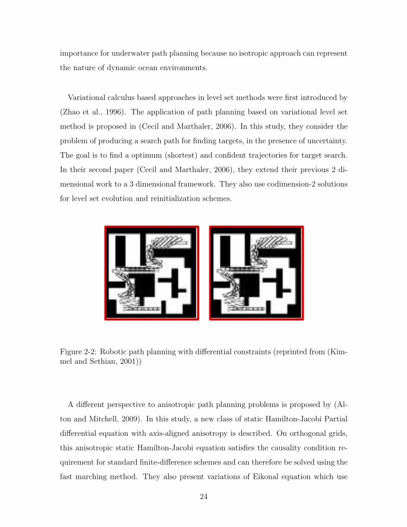
Two years later, in the work of (Kimmel and Sethian, 2001), the robotics path
planning in the presence of differential constraints was introduced. Therefore, the
fast marching approach became no longer constrained to point body dynamics, and
it becomes practical tool in path planning for robotics. Please see Figure 2-2. Another
very important step in path planning by using anisotropic approach, based on fast
marching method, is proposed in (Sethian and Vladimirsky, 2000). This has special
23
importance for underwater path planning because no isotropic approach can represent
the nature of dynamic ocean environments.
Variational calculus based approaches in level set methods were first introduced by
(Zhao et al., 1996). The application of path planning based on variational level set
method is proposed in (Cecil and Marthaler, 2006). In this study, they consider the
problem of producing a search path for finding targets, in the presence of uncertainty.
The goal is to find a optimum (shortest) and confident trajectories for target search.
In their second paper (Cecil and Marthaler, 2006), they extend their previous 2 di-
mensional work to a 3 dimensional framework. They also use codimension-2 solutions
for level set evolution and reinitialization schemes.
Figure 2-2: Robotic path planning with differential constraints (reprinted from (Kim-mel and Sethian, 2001))
A different perspective to anisotropic path planning problems is proposed by (Al-
ton and Mitchell, 2009). In this study, a new class of static Hamilton-Jacobi Partial
differential equation with axis-aligned anisotropy is described. On orthogonal grids,
this anisotropic static Hamilton-Jacobi equation satisfies the causality condition re-
quirement for standard finite-difference schemes and can therefore be solved using the
fast marching method. They also present variations of Eikonal equation which use
24

L1, L2, and L-infinity norms on orthogonal grid domains of varying node spacing and
arbitrary dimension. See Figure 2-3.
Figure 2-3: From left to right L1, L2, and L-infinity norms contours (reprinted from(Alton and Mitchell, 2009))
Today, researchers of robotics and image processing areas are increasingly incor-
porating level set and fast marching based approaches based approaches into path
planning algorithms. With the increasing developments in mathematical techniques
and computer technology, there is no doubt that these approaches will continue to
stay as one of the main focus of the researchers. Because of the huge potential of the
studies in robotics and image processing fields for the underwater path planning, the
researchers, who are working on underwater path planning, should carefully follow
developments in these fields. In the next section, we will review the path planning
algorithms for AUVs based on level set and fast marching methods.
2.4 Underwater Path Planning with Level Set and
Fast Marching Methods
Due to the highly dynamic nature of the sea, underwater path planning needs
anisotropic cost functions. An anisotropic approach for underwater path planning
using fast marching method was first introduced by (Petres et al., 2007) . The im-
portant aspects of this proposed anisotropic approach are that the curvature of the
25

final trajectory is constrained, which makes it possible to take differential constraints
into account; new quadratic upwind finite difference scheme is developed. Therefore,
directional constraints, such as ocean currents, can be taken into account. In order
to handle the real-time constraints of underwater path planning and to speed up
the computation time, multi-resolution grid system is applied to the new quadratic
upwind difference scheme.
Basically, the proposed algorithm of (Petres et al., 2007) hinges on solving the
Eikonal equation with anisotropic cost function τ . The cost function τ can be thought
as the slowness of the vehicle at each point in the domain. The Eikonal equation
together with the anisotropic cost function τ is stated as follows;
||∇µ|| = τ (2.1)
where µ : Ω2 → <+ is distance function to minimize, and τ is dependent on the field
force (currents)−→U .
In order to handle currents, anisotropic cost function τ is split into two parts as
in Equation-2.2. The first right hand term of the Equation-2.2 handles the isotropic
constraints on the solution domain, and the second right hand term handles the
anisotropic cost function that handles forces of the solution domain, such as ocean
currents. τobst can be seen as standard isotropic cost function as in isotropic fast
marching method. The details about isotropic cost function in fast marching method
are given in Chapter-3. The anisotropic part of the cost function τ proposed by Petres
et al is stated in Equation-2.3.
τ = τobst + τvect (2.2)
τvect(i, j) = α
1− 〈∇µi,j,−→Ui,j〉
Qi,j
(2.3)
26

where Qi,j = (τabst(i, j) + 2α)supΩ||−→U || is a normalization term, and the α represents
the gain. Basically, the second term of the cost function τvect means that fields forces,
such as the ocean currents, favor the vehicle propulsion when they are in the same
direction.
As it can be seen from Equation-2.3, the proposed cost function is insufficient to
handle nonlinear reaction of the underwater vehicles to ocean currents. Examples are
given only for the linear reaction cases. Please see Figure 2-4 and 2-5. Another
limitation of this approach is that it can not cope with ocean fields in which ocean
currents have higher velocity than underwater vehicle’s velocity (Soulignac et al.,
2008). In addition to this, (Petres et al., 2007) mention neither any utilization of the
ocean prediction system nor the applicability of their approach to the ocean model
domains.
Figure 2-4: a) Isotropic b) Path planning in the presence of currents (reprinted from(Petres et al., 2007))
Another approach, which focuses on collision avoidance and utilizes the work of
(Petres et al., 2007), is proposed by (Evans et al., 2008). This study is composed of
three parts (layers). These are the sensor layer, scenario layer, and reactive layer. The
27

Figure 2-5: a) No field forces b) Path planing in the presence of currents (reprintedfrom (Petres et al., 2007))
main function of the sensor layer is to generate a local map of the operation field and
to feed the scenario layer. The Scenario layer takes these local maps and incorporate
these local maps in its previously programmed scenarios to produce feasible collision
free paths. The reactive layer utilizes the fuzzy information coming from sensor and
the scenario layers to generate safe paths in case of dire emergency conditions.
The gradient of the cost function is calculated by utilizing approach of (Petres et al.,
2007), and the cost function throughout the domain is defined as in Equation-2.4.
µ = min∫ L
0τ(C(s))ds (2.4)
where C represents all the trajectories that connect start point to destination point in
domain, and τ is the cumulative cost of these trajectories with length L. Therefore,
the Eikonal equation relating to the cost function stated in Equation-2.4 is given as
in Equation-2.5.
|∇µ| = τ (2.5)
28

In the solution approach, (Evans et al., 2008) extended the fast marching algorithm
by incorporating heuristics from A* algorithm and incremental search methods from
lifelong planning adapted from (Koenig et al., 2004). This new extended algorithm
is called Lifelong Planning Fast Marching (LPFM*). One practical result produced
by this algorithm is that when the configuration space, which is mapped onto local
maps, is modified by the sensor layer, there is no need for re-calculation of the path
while AUV is operating. Trajectory generator of this approach re-utilizes previous
calculations, and calculations are needed to be carried out just for modified region.
Examples from (Evans et al., 2008) are given in Figure 2-6.
Figure 2-6: Path planning with lifelong Fast Marching Method (reprinted from (Evanset al., 2008))
A level set based approach for the path planning is proposed by (Xu et al., 2009).
The aim of this proposed approach is to propose a minimum risk trajectory plan-
ning method that relaxes the computational cost of path planning based on level
set method in case of new obstacle detection while operating AUVs. This approach
does not consider dynamics of the vehicle. It is assumed that collision risks in the
operation region are detected by on-board limited range sensors. At every grid point,
the cost function, which drives motion of the front in the normal direction, is defined
according to the probability that indicates the risk of collision.
29

In this work, the computational cost of the path planning algorithm is reduced with
two ways. First, it is assumed that if there is no risk of collision, previously planned
trajectories remains optimal. Second, if an obstacle that creates risk of collision
is detected, level set solution is only re-produced for this portion of the domain,
and it is shown that this still gives optimal collision free trajectories. Underwater
environments, such as riverine systems, are the main motivation of this work, and
examples are given in Figure 2-7 and 2-8 .
Figure 2-7: Level set contours without obstacles (reprinted from (Xu et al., 2009))
An elegant utilization of level set and fast marching methods for the objective anal-
ysis of ocean fields was developed by Multidisciplinary Simulation, Estimation and
Assimilation System group at MIT, and it is proposed in (Agarwal, 2009). Objective
analysis is a method to create a set of consistently gridded ocean fields from sparse
observations (Bretherton et al., 1976). In this study, fast marching and level set meth-
ods are utilized for the estimation of length of optimal shortest sea paths to develop
novel objective analysis scheme for complex coastal regions and archipelagos (chain
or cluster of islands). A novel fast marching method based approach for estimation of
30

Figure 2-8: Path planning with detected obstacles (reprinted from (Xu et al., 2009))
absolute velocity under geostrophic balance in complex, multiply-connected coastal
domains is presented. It is also demonstrated that proposed approach is more efficient
and accurate than stochastically forced differential equations approach.
This section has reviewed the existing art related to the underwater path planning
for AUVs. Underwater path planning other than level set based approaches and level
set based path planning approaches for robotics and image processing are introduced
in the sub-sections 2.2 and 2.3. The studies reviewed here were selected because of
their contributions to the underwater path planning and the fact that they exploit
the stated methods, such as genetics algorithms, etc., in an interesting and unique
way.
The writer of this thesis believes that level set framework for the path planning in
an ocean like environments has promising potential for the future. Even though the
introduced techniques for the level set based path planning in this section have some
important disadvantages, the level set based approach has a huge potential for being
one of the best methodology for the path planning in an ocean-like environments,
and as it is stated before, one objective of this thesis is to to contribute to this.
31

The future use of level set based path planning in control of autonomous underwater
vehicles is tied fundamentally to general advances in mathematical theory and com-
puter technology. Due to the large mathematical nature of the level set based path
planning, developments that arise in applied mathematics in one area are likely to
provide benefits to the level set based path planning. The continued progress in com-
puter technology and applied mathematical techniques will permit further realization
of the level set based path planning. A challenge in ocean-like 4D environments is
the large amount of computational-time required to reach a desired solution. On the
other hand, the increasing availability of cheap, high-performance computing tools,
coupled with advancements in mathematical techniques, will undoubtedly provide
great benefit. In addition to increasing the effectiveness of the technique for level set
based path planning techniques, developments in the field of applied mathematics
should also make new level set based path planing methods for an ocean like environ-
ments possible, such as the narrow-band level set method (Adalsteinsson and Sethian,
1995), semi-lagrangian fast marching algorithms for optimal control , which is called
Buffered Fast Marching Method (Cristiani, 2009), and the stochastic formulation of
the level set method and its combination with filtering algorithms, such as (Osher
and Paragios, 2003), (Soner and Touzi, 2002), and (Paragios and Deriche, 2002).
32

Chapter 3
Level Set Method Theory
3.1 Introduction
The aim of this chapter is to provide an introduction to the theory used in this
thesis, and the theory of the level set method in particular. Level set method is a
computational technique to simulate the evolution of the interfaces and is an approx-
imation of solutions to the Hamilton-Jacobi type partial differential equations. It
was first introduced by Osher and Sethian (Osher and Sethian, 1988). It can easily
simulate the changing topology of the interfaces by parameterizing this interfaces in
a higher dimensional space. It has been applied to many different fields such as fluid
mechanics (Sussman and Puckett, 2000), computer graphics (Malladi et al., 1995),
applied physics (Ki et al., 2001), geosciences (Agarwal, 2009), (Lermusiaux et al.,
2011), and (Gout and Guyader, 2006), and robotics (Hassouna et al., 2005). In level
set context, there are two different formulation of interface evolution. First formula-
tion is the initial value formulation which is known as the classical level set method,
and the second formulation is boundary value formulation which is known as the fast
marching method. We will begin our discussion with classical level set method, and
then fast marching method will be discussed. The discussion in this chapter is based
on (Osher and Fedkiw, 2003)
33

3.2 Level Set Method
3.2.1 Formulation of Time-Dependent Front Evolution in the
Normal Direction
The Eulerian approach proposed by level set methodology is to embed evolving
fronts as zero level set of a N dimensional function φ to represent the motion of N-1 (co-
dimension 1) dimensional hypersurface. For the 2 dimensional case, let φ(x, y, t = 0),
where (x,y) defines the grid locations in 2 dimensional space.
φ(x, y, t = 0) = ±d (3.1)
where d is the distance form zero level set Γ(t = 0). The sign in front of the d is
negative if the grid location (x,y) is inside the initial zero level set Γ(t = 0), and
opposite otherwise. Therefore, the initial function φ(x, y, t = 0) : R2 → R has a
property on the interface that
Γ(t) = (x, y) : φ(x, y, 0) = 0 (3.2)
where Γ represents the closed interface curve bounding a open region Ω, φ is
known as the signed distance function, and φ is assumed to take negative values
inside the bounded region, and positive values outside the bounded region, and these
are represented by Ω− and Ω+ respectively. Therefore, the signed distance function
on the level set solution domain has the following properties.
φ(x, y, t) < 0 for(x, y) ∈ Ω−
φ(x, y, t) > 0 for(x, y) ∈ Ω+
φ(x, y, t) = 0 for(x, y) ∈ Γ(t)
34

Now, the goal is to come up with an equation to represent evolving function
φ(x, y, t) which includes the embedded evolution of the Γ(t) as the zero level set of φ.
In order to match the zero level set of the evolving function φ with the propagating
front Γ, we must have
φ(x, y, t) = 0 (3.3)
and by the chain rule
φt +∇φ(x, y, t) ·X ′(t) = 0 (3.4)
where X(t)=(x(t),y(t)), Since unit normal vector to the evolving front is defined as
−→n = ∇φ|∇φ| , and Vn(X(t)) = Xt · −→n , given φ(X, t = 0), the evolution equation, also
known as level set equation, can be written as
φt + Vn|∇φ| = 0 (3.5)
Since the domain coordinate system is fixed, this solution is known as the Eulerian
formulation of the front propagation. See Figure 3-1 for the demonstration evolving
circle.
Figure 3-1: Evolving circle (reprinted from (Sethian, 1996b))
35
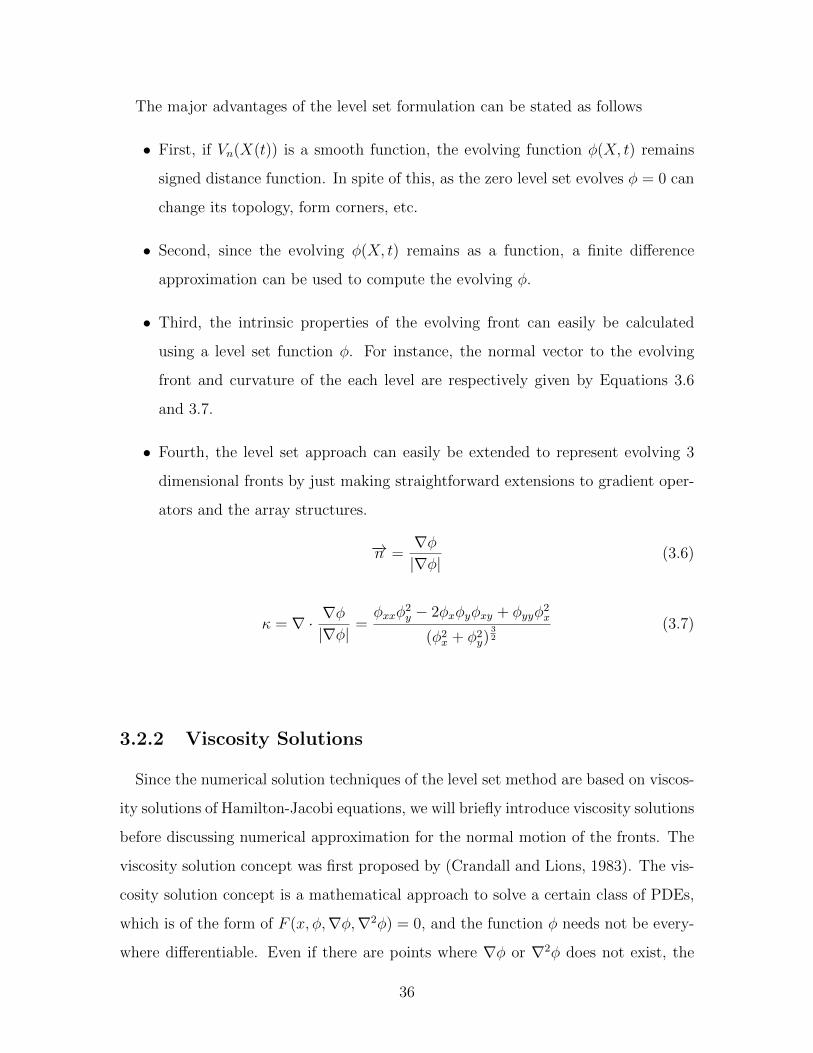
The major advantages of the level set formulation can be stated as follows
• First, if Vn(X(t)) is a smooth function, the evolving function φ(X, t) remains
signed distance function. In spite of this, as the zero level set evolves φ = 0 can
change its topology, form corners, etc.
• Second, since the evolving φ(X, t) remains as a function, a finite difference
approximation can be used to compute the evolving φ.
• Third, the intrinsic properties of the evolving front can easily be calculated
using a level set function φ. For instance, the normal vector to the evolving
front and curvature of the each level are respectively given by Equations 3.6
and 3.7.
• Fourth, the level set approach can easily be extended to represent evolving 3
dimensional fronts by just making straightforward extensions to gradient oper-
ators and the array structures.
−→n =∇φ|∇φ|
(3.6)
κ = ∇ · ∇φ|∇φ|
=φxxφ
2y − 2φxφyφxy + φyyφ
2x
(φ2x + φ2
y)32
(3.7)
3.2.2 Viscosity Solutions
Since the numerical solution techniques of the level set method are based on viscos-
ity solutions of Hamilton-Jacobi equations, we will briefly introduce viscosity solutions
before discussing numerical approximation for the normal motion of the fronts. The
viscosity solution concept was first proposed by (Crandall and Lions, 1983). The vis-
cosity solution concept is a mathematical approach to solve a certain class of PDEs,
which is of the form of F (x, φ,∇φ,∇2φ) = 0, and the function φ needs not be every-
where differentiable. Even if there are points where ∇φ or ∇2φ does not exist, the
36

viscosity solutions satisfy the given properties of the PDE, and it gives solution to the
given PDE. Therefore, uniqueness and existence theorems hold. In addition to that,
viscosity solution concept leads to stabile numerical solutions of the given PDE. It
has especially been applied to PDEs arising in optimal control and differential games,
where continuous solutions do not exist (Fleming and Soner, 2006). Since, in our
path planning framework, we are interested in solving the first order Hamilton-Jacobi
type equations, our objective PDE takes the form of Equation 3.8.
F (x, φ,∇φ) = 0 x ∈ Ω ⊆ <n (3.8)
One of the best known approaches to solve the PDEs of the form of Equation 3.8
is the method of characteristics. However, local smooth solutions produced by this
technique cannot be applied to whole solution domain Ω. In fact, singularity occurs
if the two or more characteristic front coincide at the same point on the domain Ω
(Giga, 2006)
Even though the function φ is not continuous or differentiable over the entire do-
main, we can solve Equation 3.8 by utilizing the viscosity solution technique. Let
ε → 0+. The idea of the viscosity solution technique is that the solutions φε of the
parabolic PDE problem of the form of the equation below converge to a unique limit
of φ (Crandall et al., 1992).
F (x, uε,∇φε) = ε∆φε (3.9)
At each point on the domain where φ exists, characterization of the limit function
φ can be made by applying certain inequalities on its super and sub-differentials. See
Figure 3.1. On the open set ⊆ <n, let φ : → < be a scalar function and the p.= ∇φ.
The super-differential and sub-differential sets of φ at the point X is defined as in the
Equation 3.10 and 3.11 respectively (Bressan and Piccoli, 2007).
37

D+φ(X) =
(p ∈ <n; lim sup
Y→X
φ(Y )− φ(X)− p · (Y −X)
|Y −X|≤ 0
)(3.10)
D−φ(X) =
(p ∈ <n; lim inf
Y→X
φ(Y )− φ(X)− p · (Y −X)
|Y −X|≥ 0
)(3.11)
Figure 3-2: Super and Sub-Differential of φ (reprinted from (Bressan and Piccoli,2007))
Namely, for every point X ∈ Ω and p ∈ D+φ((X), the function φ is a viscosity
subsolution of the Equation 3.8 if F (X,φ(X), p) ≤ 0, and for every point X ∈ Ω
and p ∈ D−φ((X), the function φ is a viscosity subsolution of the Equation 3.8 if
F (X,φ(X), p) ≥ 0.
Since we are interested in the time-dependent formulation of the front evolution,
we define Hamiltonian H = H(X,φ,∇φ, t). Note that second term Vn|∇φ| of the
Equation 3.5 is of this type.
φt +H(X,φ(X),∇φ, t) = 0 (3.12)
Therefore, by applying similar definitions stated above to the Equation 3.12, we
obtain the following statements;
38

• If for every point X ∈ Ω, a function ϕ = ϕ(X, t) such that φ− ϕ has a relative
minimum at (X,t), the function φ is a viscosity super-solution of Equation 3.12.
Therefore, Equation 3.13 holds
ϕt +H(X,φ,∇ϕ, t) ≥ 0 (3.13)
• If for every point X ∈ Ω, a function ϕ = ϕ(X, t) such that φ− ϕ has a relative
maximum at (X,t), the function φ is a viscosity sub-solution of Equation 3.12.
Therefore, Equation 3.14 holds
ϕt +H(X,φ,∇ϕ, t) ≤ 0 (3.14)
Now, we will discuss the existing approaches to numerically characterize and dis-
cretize the viscosity solution approach. For references, we refer first to (Crandall and
Lions, 1984), where monotone first-order approach is proposed. Later, in the work of
(Osher and Sethian, 1988), higher order method was developed by utilizing the con-
nections between conversation laws and Hamilton-Jacobi type PDEs. In this thesis,
Godunov method, which is proposed in (Godunov, 1959), is used for the characteri-
zation of the motion in the normal direction. Despite the difficulties in implementing
this method, it can properly characterize and satisfy the viscosity solution approach.
3.2.3 Numerical Discretization of the Front Evolution in the
Normal Direction
In this thesis, we utilize the normal motion of the evolving front for representing
the AUVs motion (assuming that there is no field force) from a given starting point
on the φ(X, t = 0) to the any point on the φ(X, t = tf ). We utilize the Godunov
method to characterize this front evolution in the normal direction.
39

The Godunov method is an exact numerical solution technique for the Riemann
problem. Before we give the multi-dimensional formulation of Gudonov method for
Hamilton-Jacobi type equations, definitions are given. Let D+, D−, and Do be first
order forward-difference, backward-difference, and the second order central-difference
operators respectively. Therefore, the forward and the backward finite difference
approximations for the differentiation of the signed distance function φ is given as
∂φ
∂x≈ φi+1 − φi
∆x(3.15)
∂φ
∂x≈ φi − φi− 1
∆x(3.16)
∂φ
∂x≈ φi+1 − φi− 1
2∆x(3.17)
Let Ix and Iy be intervals such that Ix = [φminx , φmaxx ] and Iy = [φminy , φmaxy ]. Let also
define extxH and extyH as follows. For all φx ∈ Ix
extxH =
min(H) if D−φx < D+φx
max(H) if D+φx < D−φx
H otherwise
Similarly, for all φy ∈ Iy
extyH =
min(H) if D−φy < D+φy
max(H) if D+φy < D−φy
H otherwise
By using the definitions above, the Multi-dimensional (in 2 dimensions) formulation
of the Godunov scheme for Hamilton-Jacobi type equations can be written as
H = extxextyH(φx, φy) (3.18)
40

Basically, the statement made by Equation 3.18 can be described as follows. For
the sake of brevity, we will consider one dimensional case. Assuming Vn > 0, H
is minimized by extxH if D−φx , D+φx are both positive and D−φx < D+φx. H is
maximized by extxH if D−φx , D+φx are both positive and D−φx > D+φx. Similarly,
extxH if D−φx , D+φx are both negative and D−φx < D+φx. H is maximized by
extxH if D−φx , D+φx are both positive and D−φx > D+φx. In the first case, we
choose D−φx, and in the second case, we choose D+φx, which are consistent with
upwinding, Now, consider the case that a kink occurs, H is minimized by extxH if
D−φx < 0 , D+φx > 0, and D−φx < D+φx. This minimization is achieved by setting
Dφx = 0. H is maximized by extxH if D−φx > 0 , D+φx < 0, and D−φx > D+φx.
This minimization is achieved by taking the maximum magnitude of D−φx and D+φx.
Even though the Godunov method is difficult to implement, because of its success to
handle artificial dissipation and to characterize the viscosity solution of front evolution
problem, it was chosen for this thesis work. In summary, It can be summarized as
follows: for both positive or negative Vn
Dφx =
D−φx if VnD−φx > 0 and VnD
+φx > 0
D+φx if VnD−φx < 0 and VnD
+φx < 0
0 if VnD−φx ≤ 0 and VnD
+φx ≥ 0
max(|VnD−φx|, |VnD+φx|) if VnD−φx ≥ 0 and VnD
+φx ≤ 0
0 otherwise
(3.19)
In the paper ”A Viscosity Solution to Shape from Shading”, (Rouy and Tourin,
1992) proposed the scheme given in Equation 3.19 which elegantly characterizes the
Godunov method.
41

Dφ2x =
max(max(D−φx, 0)2,min(D+φx, 0)2) if Vn > 0
max(min(D−φx, 0)2,max(D+φx, 0)2) if Vn < 0(3.20)
3.2.4 Front Evolution Due to Field Forces
In addition to our underwater vehicle speed which is characterized by front evolu-
tion in the normal direction, since underwater vehicles are subject to field forces such
as ocean currents, the zero level set front evolution can be affected by externally gen-
erated velocity field ~V = ~V (x, y, t). If there is no normal (vehicle in drift condition)
motion but external velocity on the interface, the motion of the interface is same as
external velocity field. For instance, if the velocity field on the interface is ~V = 〈0, 1〉
, and the Vn = Vn(x, y) = 0, then the interface is only driven by external velocity field
and move up. We use the advection equation to simulate interface motion driven by
an externally generated velocity field. The advected front evolution equation is
φt + ~V∇φ = 0 (3.21)
Even though the velocity field ~V generally is defined on the whole domain Ω,
it is better to use the field values in the band containing the zero level set of the
signed distance function φ. One important advantage of band implementation is
that less steep gradients may occur far from the zero level set φ = 0 on the domain
Ω. Therefore, we need less reinitialization of our signed distance domain. For more
information, about reinitialization of the signed distance field, we refer to Subsection
3.2.8.
3.2.5 Numerical Discretization of the Front Evolution due to
Field Forces
Let’s consider the Godunov method discussed in subsection 3.2.3 again. In contrast
to front motion in the normal direction, we have separate velocities u and v in every
cartesian direction. Therefore, we can separate Equation 3.18 as follows
42
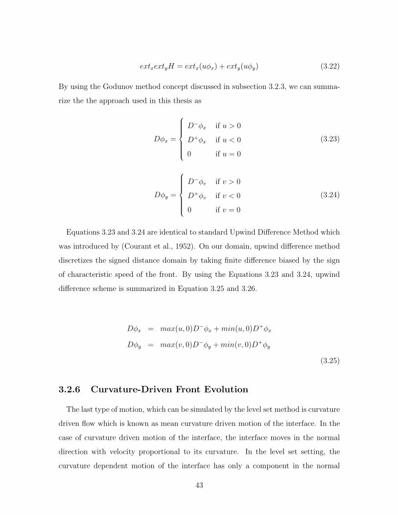
extxextyH = extx(uφx) + exty(uφy) (3.22)
By using the Godunov method concept discussed in subsection 3.2.3, we can summa-
rize the the approach used in this thesis as
Dφx =
D−φx if u > 0
D+φx if u < 0
0 if u = 0
(3.23)
Dφy =
D−φv if v > 0
D+φv if v < 0
0 if v = 0
(3.24)
Equations 3.23 and 3.24 are identical to standard Upwind Difference Method which
was introduced by (Courant et al., 1952). On our domain, upwind difference method
discretizes the signed distance domain by taking finite difference biased by the sign
of characteristic speed of the front. By using the Equations 3.23 and 3.24, upwind
difference scheme is summarized in Equation 3.25 and 3.26.
Dφx = max(u, 0)D−φx +min(u, 0)D+φx
Dφy = max(v, 0)D−φy +min(v, 0)D+φy
(3.25)
3.2.6 Curvature-Driven Front Evolution
The last type of motion, which can be simulated by the level set method is curvature
driven flow which is known as mean curvature driven motion of the interface. In the
case of curvature driven motion of the interface, the interface moves in the normal
direction with velocity proportional to its curvature. In the level set setting, the
curvature dependent motion of the interface has only a component in the normal
43

direction. Therefore, the normal velocity can be defined as ~Vc = −bκ ~N where b is a
constant and κ is a curvature given in Equation 3.7. If b < 0, the interface moves in
the direction of concavity. If b > 0 , the interface moves to the direction of convexity.
The curvature driven interface motion equation can be given as
φt + Vc∇φ = 0 (3.26)
In this thesis work, we dot not utilize the curvature-driven front evolution of the
signed distance function. Therefore, we just content ourselves with a brief discussion
of numerical characterization of the curvature-dependent signed distance function
evolution. Since the second term of the Equation 3.26 is parabolic, central finite
difference scheme is needed to characterize this equation (Malladi and Sethian, 1996),
or the second order scheme that is used in (Agarwal and Lermusiaux, 2011) can be
utilized. For the 2 dimensional case, the central difference scheme for the curvature-
dependent motion can be written as
Dφ = bκ((Doφx)2 + (Doφx)
2)12 (3.27)
3.2.7 Putting Everything together
In order to obtain general interface evolution, we put equations 3.5, 3.21, and 3.26
together. Therefore,
φt + ~V∇φ + Vn|∇φ| − Vc∇φ = 0 (3.28)
In our path planning setting, we are not interested in curvature dependent term of
the equation 3.28. Therefore, we are just interested in solving the first two terms of
the equation 3.28. Therefore, the Equation 3.28 is reduced to Hamilton-Jacobi type
PDE given in Equation 3.29, and the Equation 3.29 can be rewritten as in Equation
3.30.
44

φt + ~V∇φ + Vn|∇φ| = 0 (3.29)
φt +H(X, ~U, φ,∇φ) = 0 (3.30)
Now, we are beginning discussion of discretization of the Equation 3.30. Let H1
and H2 be H1 = u + Vnφx|∇φ|−1 and H1 = v + Vnφy|∇φ|−1 respectively. If the
signs of u and Vn are same for both D−φx and D+φx, the front moves in the same
direction with u and Vn. Therefore, by referring the Equations 3.19 and 3.23, we set
Dφx = D−φx.
Now, consider the case where u and Vn do not have same sign. This means that the
normal motion and advected motion of the front are in opposite directions. In order
to satisfy upwinding requirements, one needs to determine the dominant motion of
the front. Therefore, by referring to the Equation 3.19 and 3.23, we can make our
characterization of the front evolution in 2 dimension, as follows:
Dφx =
D−φx if H1 > 0 for both D−φx and D+φx
D+φx if H1 < 0 for both D−φx and D+φx
max(|D−φx|, |D+φx|) if H1 > 0 for D−φx and H1 < 0 for D+φx
−uVn
if H1 < 0 for D−φx and H1 > 0 for D+φx
0 otherwise
(3.31)
Dφy =
D−φy if H2 > 0 for both D−φy and D+φy
D+φy if H2 < 0 for both D−φy and D+φy
max(|D−φy|, |D+φy|) if H2 > 0 for D−φy and H2 < 0 for D+φy
−vVn
if H2 < 0 for D−φy and H2 > 0 for D+φy
0 otherwise
(3.32)
45

Note that if H1 < 0 for D−φx and H1 > 0forD+φx, we set Dφx is equal to −u/Vnbecause the Godunov method chooses the minimum value for H, and this relative
minimum occurs when H1 is equal to zero. This statement is also valid for H2.
In this thesis work, the method Godunov method is utilized to characterize the
front evolution. We define the front zero level set of the signed distance function φ.
Despite the success of Godunov method to characterize the front evolution, as the
front evolves, the signed distance function field generally looses its signed distance
property. In the next subsection, we will discuss this issue of the signed distance
function.
3.2.8 Construction and Reinitialization of the Signed Dis-
tance Field
As it is stated in the previous subsection, the signed distance function needs to be
initialized to start calculations and reinitialized during the run to avoid numerical
instabilities. In seminal work of (Osher and Sethian, 1988), the signed distance func-
tion is initialized by using φ = 1∓ d2 where the distance function d takes the minus
sign in Ω− and positive sign in Ω+. In the work of (Mulder et al., 1992), it is shown
that φ = ∓d is a better choice which gives better results than approach of (Mulder
et al., 1992).
In the work of (Chopp, 1993), the notion of reinitialization is introduced. In this
work, reinitialization is realized by stopping calculations at certain frequency and by
calculating distance of every point on the domain Ω from the zero level set contour
φ = 0. In this thesis work, reinitializations for 3 dimensional calculations is of this
type. In order to discretize and locate the zero level set of the function φ during
the 3 dimensional calculations, we utilize crossing time approach proposed for the
image processing applications in the series of papers (Bruckstein, 1988), (Kimmel
and Bruckstein, 1992), and (Kimmel and Bruckstein, 1993).
46

In order to find the zero level set front of the signed distance function φ, we find
isocontours of the crossing times. We utilize interpolation techniques to find the
crossing time isocontours if the zero level set front does not lie on the grid points.
Assume that we stop calculations at time T. This time T contour gives the zero level
set of the signed distance function φ. Then, we calculate distance every point on the
domain from time T isocontour. If the grid point crossing time tgrid is less than T ,
the distance takes negative sign. If the grid point crossing time (predefined) tgrid is
greater than T , the distance takes positive sign. Therefore, we can re-construct our
signed distance field again.
For the 2 dimensional calculations, instead of calculating every grid point distance
from the zero level set contour, we utilize fast marching approach which can accu-
rately calculate the signed distance field. More information regarding reinitialization
with the fast marching approach will be given in Section 3.3. Several reinitialization
approaches have been proposed to avoid numerical losses on the signed distance field.
For more information and recent advances about reinitialization of the level set cal-
culations, we refer the reader interested in reinitialization of the signed distance field
to (Russo and Smereka, 2000), (Sussman et al., 1994), and (Sussman and Fatemi,
1999).
3.3 Fast Marching Method
3.3.1 Introduction
Before introducing fast marching method, we should first consider Dijkstra algo-
rithm. The Dijkstra algorithm is closely related to the fast marching method. It can
be said that the fast marching method is a continuous formulation of the Dijkstra
algorithm(Sethian, 2001). Dijkstra’s algorithm, first introduced by Edsger Dijkstra
in 1956 (Dijkstra, 1959), is a graph search algorithm that finds the shortest path
between given start and terminal points on the graph. This algorithm is widely used
in robotics, computer science, and several engineering disciplines.
47

3.3.2 Dijkstra Algorithm
Now, let us give the definition of the Dijkstra shortest path algorithm. Given
weighted graph G(V,E) , the shortest path between any 2 vertex on this graph can
be found by the algorithm given below.
1. At the beginning all nodes are marked as unvisited. Set start node as current
node
2. Compute temporary distance from current node to all neighbor nodes. For
example, if the recorded distance from any neighbor node to initial node is less
than the previously recorded distance from initial node to this neighbor node,
overwrite the previously recorded distance to this neighbor node. When we are
done with checking all neighbors of the current node, mark the current node as
visited. A visited node will never be visited again, and the recorded distance of
visited node is eventual and optimum.
3. If all the nodes have been marked as visited, finish the process. Otherwise,
continue with the smallest distance as the next ”current node” and continue
from step-2.
The complexity of the Dijkstra’s Algorithm is O(M log M) . The Dijkstras Algo-
rithm gives the solution to the discrete optimal path planning problem on a given
cartesian grid. Mathematically, the Dijkstra’s Algorithm can be stated as follows
(Sethian and Vladimirsky, 2004); consider a cartesian grid domain with grid size ∆h.
The cost for crossing each grid point Xij = (i∆h, j∆h) in this domain is given as
Jij > 0. Therefore, the optimum cost function for the neighbor point of Xij, for
instance, for the point Xi+1,j can be found as follows
J(Xi+1,j) = min(f(Xi.j)c(Xi+11,j) + J(Xi,j)) (3.33)
where f is weight associated with the point Xi,j, c is cost to go from Xi,j to Xi+ 1, j/,
and J(Xi,j) is minimum accumulated cost at the point Xi,j.
48

3.3.3 Fast Marching Algorithm
Fast marching algorithm is a numerical method to solve the nonlinear Eikonal equa-
tion. On the rectilinear grid domain which has M grid points, analogously, the com-
plexity of the fast marching algorithm is O(M log M) (Sethian, 2001). Dijkstra-like
continuous viscosity solution formulation approach for solving the Eikonal equation
is proposed in the seminal papers of (Tsitsiklis, 1994) and (Tsitsiklis, 1995). Then,
in the paper of (Sethian, 1996a), the upwind difference method is proposed to char-
acterize viscosity solution approach proposed in (Tsitsiklis, 1995) and fast marching
idea is shown. For more information, we refer to (Sethian and Vladimirsky, 2004).
It can be said that fast marching is a stationary and continuous formulation of the
front evolution characterized by Eikonal Equation. See Equation 2.1. The term τ in
the Equation 2.5 can be considered as the term f(X)c(X) in the equation 3.33. As
in Dijkstra algorithm, the upwind difference operator with signed distance function φ
decides which grid point to update first (Step-2 of Dijkstra Algorithm) by solving the
Eikonal Equation. This continuous update is realized by the viscosity solution which
is characterized by the upwind difference method. For the two dimensional case, the
upwind difference method used for the fast marching algorithm is given in Equation
3.34 (Sethian and Vladimirsky, 2000). Note that the µ becomes µ = T in this case.
max(D−Tx,−D+Tx, 0)
max(D−Ty,−D+Ty, 0)
= τ (3.34)
The algorithm for the fast marching method can be stated as follows
1. Mark all the neighbor points which are lies on and inside initial front as accepted,
and mark all the other points in the domain as considered. See Figure 3-3.
2. Mark all the points close to the front as trial. If the points in the trial set are
49

far from the front remove them and put them back to the set of considered,
form a narrow band as in the Figure 3-3.
3. Mark trial points to set of accepted points.
4. Recalculate the values of T at all neighbors of Trial points by using Equation
3.34.
5. Return to second step of the algorithm.
Figure 3-3: Fast Marching Algorithm; red points represents set of accepted points,blue Points represents set of trial points
Fast marching algorithm has been used in many different areas such as geosciences
(Agarwal and Lermusiaux, 2011), medical imaging (Parker et al., 2002), etc. It is
faster than level set method, and implementation is not complicated. One drawback
of the fast marching algorithm is that it can only be used for fronts evolving in the
outward or inward, but not in the both direction. However, for the purpose of re-
constructing signed distance field, fast marching method is the accurate way of doing
it. Therefore, we utilize it for the reinitialization of the signed distance field of the
two dimensional path planning calculations.
50

3.3.4 Reinitialization of the Signed Distance Field with Fast
Marching
Unfortunately, the signed distance function looses its signed distance property after
a certain time step. The frequency of reinitialization depends on calculation and are
determined by experience. The idea of reinitialization with fast marching algorithm
is stated as follows.
• At certain time steps, stop level set calculations
• Solve the Equation 3.35 and evolve front in the outward direction, using points
that lie on the zero level set φ = 0 as the initial accepted points. Note that
interpolation is needed if the zero level set does not lie on the grid points.
|∇φini| = 1 (3.35)
• Solve the Equation 3.35 and evolve front in the inward direction, using points
that lie on the zero level set φ = 0 as the initial accepted points. Again,
interpolation is needed if the zero level set does not lie on the grid points.
• Set φ = φini
• Continue level set calculations.
3.4 Backward Calculations
In this section, since one of the steps of our path planning algorithm includes back-
wards computation for finding contour normal curves, We will discuss solution method
we used in this thesis. Along the level set calculations, we record history of level set
motion by recording crossing times. Therefore, at the end of the calculations we have
crossing time contours characterized by Tcross. This is a major new contribution of
this work. Examples of crossing time contours are given in Chapter 4 Section 4.3.
51

In order to find normal to these contours, we solve the following ordinary differential
equation (ODEs).
Xt = ∇Tcross (3.36)
There are many different approach for integration of ODEs, such as the Runge-
Kutta method, Leapfrog integration for initial value problems, and collocation meth-
ods for boundary value problems (Hoffman, 2001). In this thesis work, we utilize the
Euler method to solve the Equation 3.36. The mathematical description of the Euler
method is given as follows (Ascher and Petzold, 1998). Given h′
= F (h(t), t) and
h(t0) = h0, the equation for Euler method
hn+1 = hn + ∆tF (h(tn), tn) (3.37)
where ∆t is time step. Note that the Equation 3.37 shows the forward solution, but
in our algorithm, we solve it backwards in time.
In this chapter, we have discussed all the necessary mathematical background to
produce our path planning solution. In the next chapter, we will begin presenting
our algorithm based on the information given in this chapter.
52

Chapter 4
Underwater Path Planning
4.1 Introduction
The aim of this chapter is to present the path planning algorithm based on the
theory given in Chapter 3 and its applications in computer. An advantage of this
algorithm is that there is no special implementation needed to handle strong or com-
plicated ocean currents. The path planning algorithm presented here can easily find
feasible trajectories in the presence of strong currents. It can easily characterize
non-linear response of AUVs to complicated ocean flows.
Another advantage of our algorithm is its tractability even for multi-agent based
settings. In case of AUVs deployment from different locations, the cost of the algo-
rithm increases linearly, and in case of same location deployment of AUVs, the cost is
just increased by the cost of backward calculation step of the algorithm. See Section
4.2 for backward calculation.
In this section first, we will present algorithm for the path planning. Then we
present the applications as test cases to demonstrate the abilities of our algorithm.
53

4.2 Algorithm
The basic idea of the algorithm is to represent vehicle motion by evolving a front
which is characterized by φ = 0. One of the important differences of our path planning
algorithm is backward calculations for producing feasible and optimal trajectories.
In order to find feasible trajectories, we subtract the corresponding velocity from
trajectory given by crossing time contours. The idea of subtracting velocities from the
trajectory, which is normal to the crossing time contours, is introduced by Mattheus
Ueckermann (M.S) during the discussion of the path planning problem. The path
planning algorithm for AUVs, which is the core of this thesis work, can be stated as
follows
1. Initialize the signed distance domain φ ∈ Ω as in stated in Subsection 3.2.8.
and set the vehicle speed Vn. Note that the start point of our vehicle takes the
value of φ = 0. If we work with ocean prediction system, proper scaling of the
domain Ω must be done.
2. Solve Equation 3.30 for determined time step ∆t by utilizing Equations 3.20
and 3.25 with considering Equations 3.31 and 3.32.
3. Record crossing time T of each point on the domain Ω. Return to step-2 or
at every certain frequencies of the calculation time, stop calculations and go to
step-4. If the goal point is in the Ω−, go to step-5.
4. Re-construct the signed distance field φ. For the 2 dimensional case, use Equa-
tion 3.35, considering the information given in Subsection 3.3.4. For the 3 di-
mensional case re-construct the signed distance field as it is stated in Subsection
3.2.8. Return to step-2 of the algorithm.
5. Adapt Equation 3.37 to our domain and solve it backwards in time and subtract
corresponding velocity. Continue until reaching start point.
54

4.3 Applications and Test-Cases
Test-Case1: In Test-Case 1, our AUV is deployed from x = 0, y = 0 and the goal
point is at x = 0.8, y = 0.8. The speed of AUV is 1 m/s, The speed jet flow, which
is shown as a narrow band with black arrows, is constant u=0.5 and in the direction
of +x. As it can be seen from Figure 4-1, AUV changes its trajectory angle when
it reaches flow field and takes the advantage of the flow field to optimally reach goal
point.
Figure 4-1: Test-Case 1
Test-Case2: In Test-Case 2, our AUV is deployed from x = 0, y = −0.3 and the
goal point is at x = −0.75, y = 0.75. The speed of AUV is 1 m/s, In contrast to the
55

Test-Case 1.The speed of jet flow, which is shown as narrow band with black arrows,
is higher than AUV speed and constant u=0.5 m/s, and it is in the direction of +x.
As it can be seen from Figure 4-2, AUV can find the feasible trajectory and take
advantage of the flow field even its speed is higher than AUV speed.
Figure 4-2: Test-Case 2
Test-Case3: In Test-Case 3, our AUV is deployed from x = 0, y = −0.4 and the
goal point is at x = 0, y = 0..8. The speed of AUV is 1 m/s, In this case, we have
two different jet flow. The first jet flow, which is shown as narrow band with black
arrows on the left, has a speed higher than AUV speed and constant v1 = 2m/s, and
56

it is in the direction of +y. The second jet flow, which is shown as narrow band with
red arrows on the right, has a speed equal to AUV speed and constant v2 = 1m/s,
and it is in the direction of +y. As it can be seen from Figure 4-3, AUV takes the
advantage of the higher jet flow on the right to optimally reach the goal point.
Figure 4-3: Test-Case 3
Test-Case4: In Test-Case 4, our AUV is deployed from x = −0.6, y = −0.6 and the
goal point is at x = 0.6, y = 0.6. The speed of AUV is 1 m/s, In this case, we have
two different jet flowing in the inverse directions. The first jet flow, which is shown
as narrow band above with black arrows, has a speed higher than AUV speed and
57

constant u1 = 1.5m/s, and it is in the direction of −x. The second jet flow, which
is shown as narrow band below with red arrows, has a speed higher than AUV speed
and constant u2 = 1.5m/s, and it is in the direction of +x. As it can be seen from
Figure 4-4, the AUV first finds feasible trajectory to cross jet flow below and takes
the advantage of this flow. Then, in order to optimally reach goal point, AUV takes
the advantage of the jet flow above.
Figure 4-4: Test-Case 4
Test-Case5: In Test-Case 3, our AUV is deployed from x = −0.6, y = 0.6 and the
goal point is at x = −0.6, y = −0.6. The speed of AUV is 1 m/s, In this case, we
have two different jet flow. The first jet flow, which is shown as narrow band above
with red arrows, has a speed higher than AUV speed and constant v1 = 1.5m/s, and
58

it is in the direction of +y. Therefore, it is infeasible to use any trajectory crossing
jet flow above. The second jet flow, which is shown as narrow band below with black
arrows, has a speed higher than AUV speed and constant u2 = 1.5m/s, and it is in
the direction of +x. As it can be seen from Figure 4-5, AUV first finds the optimal
trajectory, which is to flow on the right side of the narrow band above, then to cross
the jet flow below. Then, In order to optimally reach goal point, AUV takes the
advantage of the jet flow below.
Figure 4-5: Test-Case 5
Test Case 6 In this test-case, we are interested in path planning in the presence
of complicated flows. lid-driven Cavity flow was chosen to simulate complicated flow
fields. The lid-driven cavity flow is a standard test or validation flow to test new
59

developed codes (Botella and Peyret, 1998). The lid-driven flow domain has simple
2 dimensional geometry. In this thesis work, we utilized the standard case where
flow field is restricted in a square domain. Dirichlet conditions are applied to three
stationary boundary and one moving boundary. See Figure 4-6. The resultant flow
with the zero level set of φ, which is shown as turquoise curve, can be seen in Figure
4-7.
Figure 4-6: Boundaries of Lid-Driven Cavity Flow Domain
In Test-Case 6, our AUV is deployed from x = 0.5, y = 0.5 and the goal point is
at x = 0.8, y = 0.5. The speed of AUV is 0.4 m/s. The maximum speed is realized
during the simulation time in the flow domain is 0.6 m/s, which is higher than AUV
speed. As it can be seen from Figure 4-8, AUV first finds the optimal trajectory to
reach the goal point
60

Figure 4-7: Time Dependent Lid-Driven Cavity Flow with front evolution
Figure 4-8: Test-Case 6
61

Test-Case 7 In Test-Case 7, we show how the AUV can take advantage of the com-
plicated flow fields by using our path planning algorithm. The flow data used in this
case is same as Test-Case 6. In this case, our AUV is deployed from x = 0.5, y = 0.3
and the goal point is at x = 0.5, y = 0.9. The speed of AUV is 0.4 m/s. The maxi-
mum speed realized along the simulation time in the flow domain is 0.6 m/s, which
is higher than AUV speed. As it can be seen from Figure 4-9, instead of moving in
straight route to goal point, our AUV follows curve trajectory which provides feasible
trajectory and advantage of the lid-driven cavity flow field.
Figure 4-9: Test-Case 7
62

4.4 Path Planning with Ocean Prediction System
In this section, we show the path planning application combined with Ocean pre-
diction system. In our framework, the MSEAS ocean prediction system is used as
data provider for our path planning algorithm. The ocean prediction data is taken
from realistic ocean predictions based on the real-time AWACS and SW06 exercises
(Aug.Sep. 2006) in the New Jersey Shelf/Hudson Canyon region (Lermusiaux, 2006)
(Haley and Lermusiaux, 2010). The domain is a 172 155-km domain, with 1-km
resolution and 30 vertical levels. Objective analyses were used for estimation of the
initial conditions, using the data gathered by gliders, AUVs, ship deployed conduc-
tivity temperature depth (CTD) and the historical data taken from World Ocean
Database, Gulf Stream Feature analyses, National Marine Fisheries Service, etc. The
duration for this real-time ocean prediction simulation was 43.5 days. Here, we fo-
cus on the period during which Tropical Storm Ernesto passes by the region in late
August - early September, 2006.
Figure 4-10: Ocean Flow Prediction on Near Surface level
63

In order to simulate realistic and most practical conditions, we set our vehicle speed
to 0.25 m/s, which is most of the currently operated underwater gliders’ maximum
speed. The goal of vehicle is to reach the goal location from start position which are
shown in Figure 4-10. In this simulation, we use ocean prediction data of Middle
Atlantic Bight region, which is subject to tropical storm Ernesto. Therefore, if the
glider use the straightforward trajectory from start location to goal location, it is
impossible to reach goal location because of the strong ocean currents in the region.
However, by using the algorithm presented in this thesis in 3D, our glider dive into
deep, near bottom levels (80 m) of the ocean, and it takes the advantage of the flow
field in the deep ocean region. See Figure 4-11 for the near bottom flow field. Note
that the colormap shown in Figures 4-10 and 4-11 are velocities(m/s) of ocean
currents.
Figure 4-11: Ocean Flow Prediction on Near Bottom level
In this chapter, we have presented our new 3D path planning algorithm for AUVs.
As it is shown in Section 4.4, our path planning algorithm can be used in real-time
64

Figure 4-12: 3D Path Planning, red curve represents 3D Trajectory and other curvesrepresent projections on cartesian planes
operations carried out by underwater gliders and vehicles. On the other hand, the
capabilities of our path planning algorithm is not limited to underwater path planning.
It can also be used for autonomous sea surface vehicles, vehicles operated in the
atmosphere such as montgolfier balloons, or any environment that has a dynamic
flow. Other possible improvements for our path planning algorithm are discussed in
the next chapter.
65

66

Chapter 5
Conclusions
From the naval operations to the scientific missions, the importance of autonomous
vehicles is increasing with the advancing underwater robotics technology. There is
no doubt that one crucial part of these autonomous underwater missions is to pro-
duce optimal and feasible paths. The goal of this thesis is to propose an optimal,
feasible, and tractable underwater path planning algorithm which can be utilized for
autonomous underwater vehicle operations. In order to fulfill this goal, a comprehen-
sive review of existing underwater path planning and related robotics path planning
algorithms together with the advantages and disadvantages of these methods were
discussed in Chapter 2. Then, the underpinning theory of the presented underwa-
ter path planning algorithm, which is level set method, was discussed in Chapter 3.
Detailed discussion of numerical and theoretical aspects of the level set method was
made. In Chapter 4, our path planning algorithm was presented. In order to show
the capabilities of presented algorithm, many realistic and non-realistic test cases are
demonstrated. Finally, to show the real-time capabilities of our algorithm, 3D path
planning together with the Multidisciplinary Simulation Estimation and Assimilation
System (MSEAS) data was demonstrated.
We believe that level set method is a promising framework to produce optimal,
feasible, and practical solutions for underwater path planning, and the presented path
67

planning algorithm can be developed and extended in many ways. The summary of
the results and the future work suggestions are stated as follows.
5.1 Summary of Results
One of the advantage of the presented algorithm is its capability and efficiency to
handle non-linear response of the underwater vehicles to complicated time-dependent
and intermittent ocean flows. It was demonstrated that even in fully chaotic flow
environment, our algorithm can work without any need of special implementation.
Second, in addition to built-in capability of handling complicated flows, our path
planning algorithm can easily produce feasible trajectories without need of special
implementation. If the algorithm cannot produce any feasible trajectory between start
and goal points, that means there is no feasible trajectory in the problem domain.
Third, since the ocean has complicated dynamics and analytically unpredictable
behaviors, ocean prediction and simulation models, such as MSEAS, must be used in
order to produce reasonable predictions of optimal paths.. The presented algorithm
can easily work with ocean prediction system with just making minor modifications,
such as scaling and smoothing of the fronts. This was completed for an example in
the Middle Atlantic Bight region in ocean conditions corresponding to the passage of
a tropical storm.
Fourth, a very important aspect of our algorithm is that its tractability and accu-
racy even for large ocean domains and data.
Finally, in case of multi-vehicle operations, if the vehicles are deployed from same
location, the cost of our algorithm is just increased by the cost of the backwards
solution needed for each vehicle. The level set framework is open to improvements,
and many modification can be made to improve the presented algorithm. On the
68

other hand, many exciting research questions are waiting to be explored. In the next
subsection, we will discuss these open research questions and suggestions.
5.2 Suggestions and Future Work
One important constraint of real-time underwater vehicle operations is that com-
putational cost of path planning algorithms. For our path planning algorithm, the
computational cost can be decreased by implementing well-defined level set solutions,
such as narrow band level set method (Adalsteinsson and Sethian, 1995), sparse field
level set method (Whitaker, 1998), sparse block grid level set method (Bridson, 2003),
octree level set method (Strain, 1999) and (Losasso et al., 2004), run-length encoded
level set method (Houston et al., 2006) and (Nielsen and Museth, 2006), and for non-
uniform ocean data, point based level set method (Corbett, 2005). For instance, one
improvement can be made by implementing narrow band level set method. In the
narrow band implementation of the level set method, since the calculations are car-
ried out in the small band around the zero level set, the computational cost decreases
considerably.
Considerable amount of computational cost of our path planning algorithm comes
from the reinitialization of the signed distance domain. Instead of implemented reini-
tialization approaches used for this thesis work, more efficient reinitialization schemes
can be used for decreasing the computational cost of our path planning algorithm,
such as method proposed in (Sussman et al., 1994). On the other hand, determining
the frequency of reinitialization during the path planning calculations is still open
research question. There is no doubt that if ideal forms of reinitialization are deter-
mined, this will lead to more efficient autonomous underwater vehicle operations.
Another open research question is to develop fully consistent level set numerical
scheme to combine path planning algorithm with the ocean prediction system. In ad-
dition to that, combining stochastic ocean predictions with our path planning schemes
69

remains as exciting research subject. Currently, The Multidisciplinary Simulation Es-
timation and Assimilation System Group of MIT is exploring this promising research
question.
70

Appendix A
Description of Matlab Files
A.1 Matlab Scripts for Two Dimensional Calcula-
tions
cavitypathplanning.m (Function) : This matlab function conducts path plan-
ning in the presence of cavity flow. It uses cavity flow data supplied by the user. It can
also be used for other data without need of special implementation. Note that data
must be in the search directory of Matlab. The structure of cavitypathplanning.m
function is stated as follows.
cavitypathplanning.m(rx0,ry0,rx,ry)
where rx0 is cartesian x coordinate of start point, ry0 is cartesian y coordinate of
start point, rx is cartesian x coordinate of goal point, and ry is cartesian y coordinate
of goal point.
pathplanning2d.m (Script) : This Matlab script conducts two dimensional ide-
alized test cases. In order to make changes in flow field, code must be modified.
71
A.2 Matlab Scripts for Three Dimensional Calcu-
lations
readvelodata.m(Function) : This Matlab function reads MSEAS data and puts
it into path, and it reads velocity components at every time step from given ocean
prediction data. The structure of this Matlab function is stated as follows.
[u, v, w, a] = readvelodata(xgridnumber, ygridnumber, zgridnumber, time, speed, recnum, ncid)
where xgridnumber is number of grid points in the cartesian x direction, ygridnumber
is number of grid points in the cartesian y direction, zgridnumber is number of grid
points in the cartesian z direction, time is number of ocean forecast step, speed is
the speed of AUV, ncid is the name of ocean prediction data formatted as netcdf.
The outputs of this functions are stated as follows. u is cartesian x component of the
velocity field, v is the cartesian y component of the velocity field, w is the cartesian
z component of the velocity field, a is the normal velocity field of the wave front.
vertface2obj.m (Function) : For visualization purposes, this function saves co-
ordinates of vertices of faces as a Wavefront (.Obj) file. The structure of this Matlab
function is stated as follows
vertface2obj(v, f, name)
where v is a Nx3 matrix of vertex coordinates, f is a Mx3 matrix of vertex indices,
and fname is the filename to save the obj file.
setdomain.m (Script) : This Matlab script initializes signed distance domain
required for level set path planning
setoperators.m (Script) : This Matlab script initializes the differential operators
and field forces matrices.
72

mseaspathplanning3d.m (Function) : This Matlab function is the main func-
tion that carries out the path planning calculations. It conducts numerical calcula-
tions and reinitialization of the signed distance field. The structure of this function
is stated as follows.
mseaspathplanning3d(flowfield, xgridnumber, ygridnumber, zgridnumber, recnum, speed, start, target, saveobj)
where flow field is optional flow field structure, and by default it is input as ”[]”,
xgridnumber is number of grid points in the cartesian x direction, ygridnumber is
number of grid points in the cartesiany direction, zgridnumber is number of grid
points in the cartesian z direction, recnum is the number ocean forecast step, start is
the start point of underwater vehicle, target is the goal point of underwater vehicle,
saveobj is the name of the data file which is saved for the visualization purposes.
savevtkfile.m (Script) : This script creates animations file directory, and calls
vertface2obj function to create wavefront (.obj) data.
savevtkvector.m (Function) : savevtkvector.m function saves a 3-D vector of
any size to filename in VTK format. X, Y and Z should be arrays of the same size,
each storing speeds in the a single cartesian directions. The structure of this function
is stated as follows
savevtkvector (readfile,filename)
where readfile is the name of dat file in which we save three dimensional velocity data,
and filename is the name of vtk file we would like to save.
plotpath.m (Script) : This script plots the three dimensional paths. When this
script is used, four subplot are seen on screen. Three of these plots are projections
of three dimensional trajectory on to cartesian planes, and the fourth one is three
dimensional plot.
73

PlotPath (XX,YY,ZZ) (Function) : PlotPath function shows the cartesian
planes projections and three dimensional trajectory on the same plot window. The
structure of PlotPath function is stated as follows.
PlotPath (XX,YY,ZZ)
where XX is cartesian x coordinate of the trajectory, YY is cartesian y coordinate of
the trajectory, and ZZ is cartesian z coordinate of the trajectory.
74

Bibliography
Adalsteinsson, D. and Sethian, J. (1995). A fast level set method for propagatinginterfaces. Journal of computational physics, 118(2):269–277.
Agarwal, A. (2009). Statistical field estimation and scale estimation for complexcoastal regions and archipelagos. Technical report, MASSACHUSETTS INST OFTECH CAMBRIDGE DEPT OF MECHANICAL ENGINEERING.
Agarwal, A. and Lermusiaux, P. (2011). Statistical Field Estimation for ComplexCoastal Regions and Archipelagos. Submitted to Journal of Ocean Modelling.
Alton, K. and Mitchell, I. (2009). Fast marching methods for stationary Hamilton–Jacobi equations with axis-aligned anisotropy. SIAM Journal on Numerical Anal-ysis, 47(1):363–385.
Alvarez, A., Caiti, A., and Onken, R. (2004). Evolutionary path planning for au-tonomous underwater vehicles in a variable ocean. Oceanic Engineering, IEEEJournal of, 29(2):418–429.
Ascher, U. and Petzold, L. (1998). Computer methods for ordinary differential equa-tions and differential-algebraic equations, volume 61. Society for Industrial Math-ematics.
Botella, O. and Peyret, R. (1998). Benchmark spectral results on the lid-driven cavityflow. Computers & Fluids, 27(4):421–433.
Bressan, A. and Piccoli, B. (2007). Introduction to the mathematical theory of control.American institute of mathematical sciences.
Bretherton, F., Davis, R., and Fandry, C. (1976). A technique for objective analy-sis and design of oceanographic experiments applied to mode-73. Deep-Sea Res,23(7):559–582.
Bridson, R. (2003). Computational aspects of dynamic surfaces. PhD thesis, Citeseer.
Bruckstein, A. (1988). On shape from shading. Computer Vision, Graphics, andImage Processing, 44(2):139–154.
Carroll, K., McClaran, S., Nelson, E., Barnett, D., Friesen, D., and William, G.(1992). AUV path planning: an A* approach to path planning with consideration of
75

variable vehicle speeds and multiple, overlapping, time-dependent exclusion zones.In Autonomous Underwater Vehicle Technology, 1992. AUV’92., Proceedings of the1992 Symposium on, pages 79–84. IEEE.
Cecil, T. and Marthaler, D. (2006). A variational approach to path planning in threedimensions using level set methods. Journal of Computational Physics, 211(1):179–197.
Chopp, D. (1993). Computing minimal surfaces via level set curvature flow. Journalof Computational Physics, 106:77–77.
Corbett, R. (2005). Point–Based Level Sets and Progress Towards Unorganised Par-ticle Based Fluids. PhD thesis, The University of British Columbia.
Courant, R., Isaacson, E., and Rees, M. (1952). On the solution of nonlinear hy-perbolic differential equations by finite differences. Communications on Pure andApplied Mathematics, 5(3):243–255.
Crandall, M., Ishii, H., Lions, P., and Society, A. M. (1992). User’s guide to viscositysolutions of second order partial differential equations. American MathematicalSociety.
Crandall, M. and Lions, P. (1983). Viscosity solutions of Hamilton-Jacobi equations.Transactions of the American Mathematical Society, 277(1):1–42.
Crandall, M. and Lions, P. (1984). Two approximations of solutions of Hamilton-Jacobi equations. Mathematics of Computation, 43(167):1–19.
Cristiani, E. (2009). A fast marching method for Hamilton-Jacobi equations modelingmonotone front propagations. Journal of Scientific Computing, 39(2):189–205.
Dijkstra, E. (1959). A note on two problems in connexion with graphs. Numerischemathematik, 1(1):269–271.
Dorst, L. and Trovato, K. (1988). Optimal path planning by cost wave propagation inmetric configuration space. In Society of Photo-Optical Instrumentation Engineers(SPIE) Conference Series, volume 1007, page 186.
Evans, J., Patron, P., Smith, B., and Lane, D. (2008). Design and evaluation of a re-active and deliberative collision avoidance and escape architecture for autonomousrobots. Autonomous Robots, 24(3):247–266.
Fleming, W. and Soner, H. (2006). Controlled Markov processes and viscosity solu-tions. Springer.
Garau, B., Alvarez, A., and Oliver, G. (2005). Path planning of autonomous under-water vehicles in current fields with complex spatial variability: an A* approach.In Robotics and Automation, 2005. ICRA 2005. Proceedings of the 2005 IEEE In-ternational Conference on, pages 194–198. IEEE.
76

Giga, Y. (2006). Surface evolution equations: A level set approach. Birkhauser.
Godunov, S. (1959). A difference method for numerical calculation of discontinuoussolutions of the equations of hydrodynamics. Matematicheskii Sbornik, 89(3):271–306.
Gout, C. and Guyader, C. (2006). Segmentation of complex geophysical structureswith well data. Computational Geosciences, 10(4):361–372.
Haley, P. and Lermusiaux, P. (2010). Multiscale two-way embedding schemes forfree-surface primitive equations in the multidisciplinary simulation, estimation andassimilation system. Ocean dynamics, 60(6):1497–1537.
Hassouna, M., Abdel-Hakim, A., and Farag, A. (2005). Robust robotic path plan-ning using level sets. In Image Processing, 2005. ICIP 2005. IEEE InternationalConference on, volume 3, pages III–473. IEEE.
Hoffman, J. (2001). Numerical methods for engineers and scientists. CRC.
Houston, B., Nielsen, M., Batty, C., Nilsson, O., and Museth, K. (2006). Hierarchicalrle level set: A compact and versatile deformable surface representation. ACMTransactions on Graphics (TOG), 25(1):151–175.
Inanc, T., Shadden, S., and Marsden, J. (2005). Optimal trajectory generation inocean flows. In Proceedings of the American Control Conference, volume 1, page674. Citeseer.
Kanakakis, V. and Tsourveloudis, N. (2007). Evolutionary path planning and naviga-tion of autonomous underwater vehicles. In Control & Automation, 2007. MED’07.Mediterranean Conference on, pages 1–6. IEEE.
Kano, H., Egerstedt, M., Nakata, H., and Martin, C. (2003). B-splines and controltheory. Applied mathematics and computation, 145(2-3):263–288.
Ki, H., Mohanty, P., and Mazumder, J. (2001). Modelling of high-density laser-material interaction using fast level set method. Journal of Physics D: AppliedPhysics, 34:364.
Kimmel, R. and Bruckstein, A. (1992). Shape from shading via level sets.
Kimmel, R. and Bruckstein, A. (1993). Shape offsets via level sets. Computer-AidedDesign, 25(3):154–162.
Kimmel, R. and Sethian, J. (1998). Computing geodesic paths on manifolds. Pro-ceedings of the National Academy of Sciences, 95(15):8431.
Kimmel, R. and Sethian, J. (2001). Optimal algorithm for shape from shading andpath planning. Journal of Mathematical Imaging and Vision, 14(3):237–244.
77

Koenig, S., Likhachev, M., and Furcy, D. (2004). Lifelong planning A*. ArtificialIntelligence, 155(1-2):93–146.
Kruusmaa, M. (2003). Global navigation in dynamic environments using case-basedreasoning. Autonomous Robots, 14(1):71–91.
LaValle, S. (2006). Planning algorithms. Cambridge Univ Pr.
Lermusiaux, P. (2006). Uncertainty estimation and prediction for interdisciplinaryocean dynamics. Journal of Computational Physics, 217(1):176–199.
Lermusiaux, P. (2007). Adaptive modeling, adaptive data assimilation and adaptivesampling. Physica D: Nonlinear Phenomena, 230(1-2):172–196.
Lermusiaux, P., Haley Jr, P., Leslie, W., Agarwal, A., Logutov, O., and Burton, L.(2011). Multiscale physical and biological dynamics in the philippine archipelago:Predictions and processes. Oceanography, 24(1):70–89.
Lermusiaux, P., Xu, J., Chen, C., Jan, S., Chiu, L., and Yang, Y. (2010). Cou-pled Ocean–Acoustic Prediction of Transmission Loss in a Continental ShelfbreakRegion: Predictive Skill, Uncertainty Quantification, and Dynamical Sensitivities.Oceanic Engineering, IEEE Journal of, 35(4):895–916.
Losasso, F., Gibou, F., and Fedkiw, R. (2004). Simulating water and smoke with anoctree data structure. In ACM Transactions on Graphics (TOG), volume 23, pages457–462. ACM.
Malladi, R. and Sethian, J. (1996). Level set and fast marching methods in imageprocessing and computer vision. In Image Processing, 1996. Proceedings., Interna-tional Conference on, volume 1, pages 489–492. IEEE.
Malladi, R., Sethian, J., and Vemuri, B. (1995). Shape modeling with front prop-agation: A level set approach. Pattern Analysis and Machine Intelligence, IEEETransactions on, 17(2):158–175.
Mulder, W., Osher, S., and Sethian, J. (1992). Computing interface motion in com-pressible gas dynamics. Journal of Computational Physics, 100(2):209–228.
Nielsen, M. and Museth, K. (2006). Dynamic tubular grid: An efficient data structureand algorithms for high resolution level sets. Journal of Scientific Computing,26(3):261–299.
Osher, S. and Fedkiw, R. (2001). Level Set Methods: An Overview and Some RecentResults* 1. Journal of Computational Physics, 169(2):463–502.
Osher, S. and Fedkiw, R. (2003). Level set methods and dynamic implicit surfaces.Springer Verlag.
Osher, S. and Paragios, N. (2003). Geometric level set methods in imaging, vision,and graphics. Springer-Verlag New York Inc.
78

Osher, S. and Sethian, J. (1988). Fronts propagating with curvature-dependentspeed: algorithms based on Hamilton-Jacobi formulations. Journal of computa-tional physics, 79(1):12–49.
Paragios, N. and Deriche, R. (2002). Geodesic active regions and level set methodsfor supervised texture segmentation. International Journal of Computer Vision,46(3):223–247.
Parker, G., Wheeler-Kingshott, C., and Barker, G. (2002). Estimating distributedanatomical connectivity using fast marching methods and diffusion tensor imaging.Medical Imaging, IEEE Transactions on, 21(5):505–512.
Petres, C., Pailhas, Y., Patron, P., Petillot, Y., Evans, J., and Lane, D. (2007). Pathplanning for autonomous underwater vehicles. Robotics, IEEE Transactions on,23(2):331–341.
Rouy, E. and Tourin, A. (1992). A viscosity solutions approach to shape-from-shading.SIAM Journal on Numerical Analysis, 29(3):867–884.
Russo, G. and Smereka, P. (2000). A remark on computing distance functions. Journalof Computational Physics, 163(1):51–67.
Sapsis, T. and Lermusiaux, P. (2009). Dynamically orthogonal field equations for con-tinuous stochastic dynamical systems. Physica D: Nonlinear Phenomena, 238(23-24):2347–2360.
Senatore, C. and Ross, S. (2008). Fuel-efficient navigation in complex flows. InAmerican Control Conference, 2008, pages 1244–1248. IEEE.
Sethian, J. (1996a). A fast marching level set method for monotonically advancingfronts. Proceedings of the National Academy of Sciences of the United States ofAmerica, 93(4):1591.
Sethian, J. (1996b). Level set methods: Evolving interfaces in geometry, fluid mechan-ics, computer vision, and materials science, volume 1999. Cambridge UniversityPress Cambridge:.
Sethian, J. (1999). Fast marching methods. SIAM review, 41(2):199–235.
Sethian, J. (2001). Evolution, implementation, and application of level set andfast marching methods for advancing fronts. Journal of Computational Physics,169(2):503–555.
Sethian, J. and Vladimirsky, A. (2000). Fast methods for the Eikonal and relatedHamilton–Jacobi equations on unstructured meshes. Proceedings of the NationalAcademy of Sciences of the United States of America, 97(11):5699.
Sethian, J. and Vladimirsky, A. (2004). Ordered upwind methods for static Hamilton-Jacobi equations: theory and algorithms. SIAM Journal on Numerical Analysis,pages 325–363.
79

Smith, R., Kelly, J., Chao, Y., Jones, B., and Sukhatme, G. (2010). Towards im-provement of autonomous glider navigation accuracy through the use of regionalocean models. In Proceedings of the 29th International Conference on OCean, Off-shore and Arctic Engineering, pages 597–606. ASME-American Society MechanicalEngineering.
Soner, H. and Touzi, N. (2002). A stochastic representation for the level set equations.Communications in Partial Differential Equations, 27(9):2031–2053.
Soulignac, M., Taillibert, P., and Rueher, M. (2008). Adapting the wavefront expan-sion in presence of strong currents. In Robotics and Automation, 2008. ICRA 2008.IEEE International Conference on, pages 1352–1358. IEEE.
Soulignac, M., Taillibert, P., and Rueher, M. (2009). Time-minimal path planningin dynamic current fields. In Robotics and Automation, 2009. ICRA’09. IEEEInternational Conference on, pages 2473–2479. IEEE.
Strain, J. (1999). Tree methods for moving interfaces* 1. Journal of ComputationalPhysics, 151(2):616–648.
Sussman, M. and Fatemi, E. (1999). An efficient, interface-preserving level set redis-tancing algorithm and its application to interfacial incompressible fluid flow. SIAMJournal on Scientific Computing, 20(4):1165–1191.
Sussman, M. and Puckett, E. (2000). A coupled level set and volume-of-fluid methodfor computing 3D and axisymmetric incompressible two-phase flows. Journal ofComputational Physics, 162(2):301–337.
Sussman, M., Smereka, P., and Osher, S. (1994). A level set approach for computingsolutions to incompressible two-phase flow. Dept. of Mathematics, University ofCalifornia, Los Angeles.
Tan, C., Sutton, R., and Chudley, J. (2004). An incremental stochastic motionplanning technique for autonomous underwater vehicles. Proceedings IFAC CAMS,20004:483–488.
Tsitsiklis, J. (1994). Efficient algorithms for globally optimal trajectories. In Decisionand Control, 1994., Proceedings of the 33rd IEEE Conference on, volume 2, pages1368–1373. IEEE.
Tsitsiklis, J. (1995). Efficient algorithms for globally optimal trajectories. AutomaticControl, IEEE Transactions on, 40(9):1528–1538.
Vasudevan, C. and Ganesan, K. (1996). Case-based path planning for autonomousunderwater vehicles. Autonomous Robots, 3(2):79–89.
Whitaker, R. (1998). A level-set approach to 3d reconstruction from range data.International Journal of Computer Vision, 29(3):203–231.
80

Witt, J. and Dunbabin, M. (2008). Go with the flow: Optimal AUV path planning incoastal environments. In Proceedings of the Australasian Conference on Roboticsand Automation.
Xu, B., Stilwell, D., and Kurdila, A. (2009). Efficient computation of level sets forpath planning. In Intelligent Robots and Systems, 2009. IROS 2009. IEEE/RSJInternational Conference on, pages 4414–4419. IEEE.
Yang, G. and Zhang, R. (2009). Path Planning of AUV in Turbulent Ocean Environ-ments Used Adapted Inertia-Weight PSO. In 2009 Fifth International Conferenceon Natural Computation, pages 299–302. IEEE.
Zhang, W., Inane, T., Ober-Blobaum, S., and Marsden, J. (2008). Optimal trajec-tory generation for a glider in time-varying 2D ocean flows B-spline model. InRobotics and Automation, 2008. ICRA 2008. IEEE International Conference on,pages 1083–1088. IEEE.
Zhao, H., Chan, T., Merriman, B., and Osher, S. (1996). A variational level setapproach to multiphase motion. Journal of computational physics, 127(1):179–195.
81