pathloss estimation techniques for incomplete...
TRANSCRIPT
LUND UNIVERSITY
PO Box 117221 00 Lund+46 46-222 00 00
Pathloss Estimation Techniques for Incomplete Channel Measurement Data
Abbas, Taimoor; Gustafson, Carl; Tufvesson, Fredrik
Unpublished: 2014-01-01
Link to publication
Citation for published version (APA):Abbas, T., Gustafson, C., & Tufvesson, F. (2014). Pathloss Estimation Techniques for Incomplete ChannelMeasurement Data. Paper presented at COST IC1004 10th Management Committee and Scientific Meeting,Aalborg, Denmark.
General rightsCopyright and moral rights for the publications made accessible in the public portal are retained by the authorsand/or other copyright owners and it is a condition of accessing publications that users recognise and abide by thelegal requirements associated with these rights.
• Users may download and print one copy of any publication from the public portal for the purpose of privatestudy or research. • You may not further distribute the material or use it for any profit-making activity or commercial gain • You may freely distribute the URL identifying the publication in the public portalTake down policyIf you believe that this document breaches copyright please contact us providing details, and we will removeaccess to the work immediately and investigate your claim.
EUROPEAN COOPERATION
IN THE FIELD OF SCIENTIFIC
AND TECHNICAL RESEARCH
—————————————————
EURO-COST
—————————————————
COST IC1004 TD(14)10084
Aalborg, DK
26-28 May, 2014
SOURCE: Dept. of Electrical and Information Technology, Lund University, Lund,
Sweden
Pathloss Estimation Techniques for Incomplete Channel
Measurement Data
Taimoor Abbas Department of Electrical and Information Technology Lund University Lund, Sweden
Phone: + 46 46 2224902
Fax: + 46 46 129948
Email: [email protected]
Pathloss Estimation Techniques for IncompleteChannel Measurement Data
Taimoor Abbas, Carl Gustafson, and Fredrik TufvessonDept. of Electrical and Information Technology, Lund University, Lund, Sweden
Abstract—The pathloss exponent and the variance of the large-scale fading are two parameters that are of great importancewhen modeling or characterizing wireless propagation channels.The pathloss is typically modeled using a single-slope log-distancepower law model, whereas the large-scale fading is modeledusing a log-normal distribution. In practice, the received signal isaffected by noise and it might also be corrupted by interferencefrom other active transmitters that are transmitting in the samefrequency band. Estimating the pathloss exponent and largescale fading without considering the effects of the noise andinterference, can lead to erroneous results. In this paper, weshow that the path loss and large scale fading estimates can beimproved if the effects of samples located below the noise floor aretaken into account in the estimation step. When the number ofsuch samples is known, then the pathloss exponent and standarddeviation of the large scale fading can be iteratively computedusing maximum likelihood estimation from incomplete data viathe expectation maximization (EM) algorithm. Alternatively, ifthe number of samples below the noise floor is unknown, weshow that the pathloss and large scale fading parameters canbe estimated based on a likelihood expression for a truncatednormal distribution.
I. INTRODUCTION
Pathloss is the expected (mean) loss at a certain distancebetween the transmitter (TX) and the receiver (RX). A numberof pathloss models have been developed for a variety of wire-less communication systems, e.g., cellular systems, bluetooth,wifi vehicle-to-vehicle dedicted short range communicationsand mm-wave point-to-point communications, working overdifferent frequency bands ranging from hundreds of MHzto tens of GHz [1]–[4]. These models have widely beenused for the prediction and simulation of signal strengths forgiven TX-RX separation distances. Typically, pathloss modelsare developed with the help of channel measurements inrealistic scenarios. The model parameters estimated from themeasurement data are thus typically valid only for a particularfrequency range, antenna arrangement, and environment forthe target scenario.
Measurement data often has limitations in one way oranother and thus there are a number of associated challenges,which often makes the estimation and modeling of the pathlossexponent from the channel measurement data non-trivial.Therefore, special considerations must be taken into accountwhen modeling the pathloss exponent by measurement data.The examples of associated challenges are;
1) Typically samples are recorded at equi-spaced time ordistance intervals. This makes the distribution of data sam-ples to be non-uniform along logarithmic distance, i.e., the
data samples have higher concentration at larger logarithmicdistances, implying that the standard least-square (LS) ormean-square-error (MSE) estimation approaches will have ahigh weight for large distances and low weight for shorterdistances. This problem can be solved by using weightedsamples for improved prediction where weights are calculatedw.r.t. the logarithmic sampling density [5]. It is very importantto explicitly mention that if the linear or logarithmic distancesampling is used for modeling, because sample distribution isdifferent for both cases and may lead to different estimates forthe same data set.
2) The pathloss exponent and the standard deviation ofthe large scale fading are random variates that vary fromlocation to location as well for different antenna heights andfrequencies. It is important to understand these variations andtheir physical motivation.
3) In practice, the observation of the received signal powerat the receiver is limited by the system noise, i.e., the sig-nals with power below the noise floor can not be measuredproperly. Moreover, the received signal power might also becorrupted by interference from other active transmitters thatare transmitting in the same frequency band. Estimating thepathloss exponent and large scale fading based on such dataset, without considering the effects of the noise floor andinterference, can lead to erroneous results. In this paper it isshown that the path loss and large scale fading estimates canbe improved if the missing samples, which are located belowthe noise floor, are taken into account in the estimation step.Two different methods are provided that incorporate missingsamples to improve the parameter estimation, first when thenumber of missing samples is unknown and second when thenumber of missing samples is known.
In section II we describe the pathloss and basic modelingassumptions. Section III explains the parameter estimationmethods. Section IV presents results for the synthetic aswell as for the channel measurement data. Finally, SectionV summarizes the discussion.
II. PATHLOSS MODELLING
A simple log-distance power law [6] is often used to modelthe path loss to predict the reliable communication rangebetween the TX and the RX. The generic form of this log-distance power law path loss model is given by,
PL(d) = PL0 + 10n log10
(d
d0
)+Xσ; d ≥ d0 (1)
where PL0 is an estimated (measured) reference level orPL0 = 20log10(4πd0/λ) the theoretical path loss at a refer-ence distance d0 in dB calculated using free-space propagationmodel. Furthermore λ is the wavelength in meters, d is thevector of distances between the TX and the RX, n is thepathloss exponent, and Xσ is a random variable to representlarge scale fading about the distance dependent pathloss,respectively. If the effect of small scale fading is removedfrom the data set by averaging the data over the time samplescorresponding to a wide-sense-stationary region, then thevariations of the large-scale fading are typically modeled usinga zero-mean Gaussian distribution with standard deviation σ,i.e., Xσ ∼ N (0, σ2). Hence, PL(d) ∼ N (µ(d), σ2) withdistance dependent deterministic expected value,
µ(d) = PL0 + 10n log10
(d
d0
); (2)
The pathloss exponent n is an environment dependentparameter commonly provided in modeling papers, which isdetermined by field measurements. Usually, n is estimated bysimple linear regression of 10 log10(d) to the measured powervalues in dB such that the mean square error (MSE) betweenthe measured and modeled points is minimized.
For peer-to-peer communication in line-of-sight (LOS)propagation conditions it is often observed that a dual-slopemodel based on two-ray ground model, as stated in [7],can represent themeasurement data more accurately. We thuscharacterize a dual-slope model as a piecewise-linear modelwith the assumption that the power decays with path lossexponent n1 until the breakpoint distance (db) and from thereit decays with path loss exponent n2. The dual-slope model isgiven by,
PL(d) =
PL0 + 10n1 log10
(dd0
)+Xσ1, if d0 ≤ d ≤ db
PL0 + 10n1 log10
(dbd0
)+ if d > db
10n2 log10
(ddb
)+Xσ2.
(3)The typical flat earth model consider db as the distance atwhich the first Fresnel zone touches the ground or the firstground reflection has traveled db + λ/4 to reach RX. The dbcan be calculated as, db = 4hTXhRX−λ2/4
λ , where λ is thewavelength at carrier frequency fc, and hTX and hRX are theheight of the TX and RX antennas, respectively. Xσ1 and Xσ2
represent large scale fading before and after the break point.For d < db, this model is the same as the log-distance powerlaw in (1).
III. ESTIMATION
To completely model the pathloss for a given data set, wewish to estimate three main parameters of (1) or (3), i.e.,n, PL0 and σ2. The data under consideration is implicitlyassumed to be Gaussian distributed because the large-scale orlarge scale fading on top of distance dependent deterministicpathloss is Gaussian, as mentioned above. Here, we willconsider parameter estimation only for (1) where the result
can easily be extended for (3). Using (1) the data set can bemodeled as,
y = Xα+ ε, (4)
where
y =
PL(d1)PL(d2)
...PL(dL)
, X =
1 10log10(d1)1 10log10d2)...1 10log10(dL)
, ε =
ε1ε2...εL
and α =
(PL0
n
)By applying ordinary least squares, the parameter α can be
estimated as
α =(XTX
)−1XTy. (5)
Using the estimates contained in α, the variance σ2 can beestimated as
σ2 =1
L− 1(y −Xα)T (y −Xα). (6)
A. Least-Square (LS) Estimation for Truncated Data
In order to estimate the pathloss exponent and fadingvariance of data truncated by a noise floor, with an unknownnumber of missing samples, it is possible to base the estima-tion on a truncated normal distribution. Under this assumption,each data observation follows a truncated normal distribution,
yi ∼ Nc(xiα, σ2), (7)
where c denotes the noise floor level. The likelihood expres-sion for this distribution is given by
l(σ,α) =
n∏i=1
1σφ(yi−xiα
σ )
1− Φ( c−xiασ )
, (8)
where φ(·) is the probability density function for the standardnormal distribution and Φ(·) is its cumulative distributionfunction, and hence the likelihood can be written as
l(σ,α) =
n∏i=1
1√2πσ
exp(− 12σ2 (yi − xiα)2)
12 (1− erf( c−xiα√
2σ))
, (9)
where erf(·) is the error function. Using the log-likelihoodL(σ,α) = ln[l(σ,α)], the parameters σ and α are estimatedusing
arg minσ,α
{−L(σ,α)}. (10)
which is easily solved by numerical optimization of α and σ.
B. Expectation-Maximization (EM) Algorithm for TruncatedData
To estimate the pathloss exponent and variance of theincomplete data with a known number of missing samples, wemake use of the expectation maximization (EM) algorithm byDempster et al. in [8]. The iterative EM algorithm is developedto estimate the mean and standard deviation of a truncated
data set by maximizing the likelihood function based uponobserved and missing samples.
The measured channel gains have a distance dependentmean and a certain standard deviation along the distance.Therefore, we divide the measured distance dependent channelgains into log-spaced distance bins so that the mean andvariance for each bin can be estimated independently.
The data y′ ∼ N (µ, σ2) associated to each distance bin isassumed to be Gaussian distributed, whereas the true mean µand standard deviation σ are unknown. Let y′1, y
′2, ..., y
′k−l be
the detected samples of y′ and y′(k−l)+1, y′(k−l)+2, ..., y
′k be the
l undetected samples, if exist, lying below the noise floor c.The mean, µ0, and standard deviation σ0 of observed (k − l)truncated data values, without considering missing samples,can then be estimated as,
µ0 =
k−l∑i=1
y′i(k − l)
, (11)
and
σ0 =
k−l∑i=1
(y′i − µ20
(k − l). (12)
The likelihood expression for this truncated distribution isgiven by
lnL(y′, µ, σ) = l ln Φ(L)− (k − l) lnσ −k−l∑i=1
(xi − µ)2/2σ2,
(13)where Φ(L) is the cumulative distribution function of L =c − µ/σ representing the probability that an observation isless than c.
For such a left-truncated data set with a known thresholdand known number of missing samples, The EM-algorithm of[8] makes use of these observed (k − l) samples to calculateinitial estimates of µ and σ. In each iteration the expectationof the conditional likelihood function of the complete datais maximized based on the type of truncation such as left-truncation in our case. At (j + 1)th iteration, the estimates ofµ and σ are given by [9], as follows
µj+1 =
[∑k−li=1 xi +
∑ki=k−lEj(xi|xi ≤ c)
]k
, (14)
σ2j+1 =
[∑k−li=1 xi − µj
2 +∑li=1Ej((xi − µj)2|xi ≤ c)
]k − 1
,
(15)where
Ej(xi|xi ≤ c) = µj − σj [φ(Lj)/Φ(Lj)], (16)
Ej((xi−µj)2|xi ≤ N0) = σj2(1−Lj [φ(Lj)/Φ(Lj)]), (17)
withLj = (c− µj)/σj . (18)
Hence, the iterative EM-algorithm improves the estimationof µ and σ in each iteration, where all of the non-detected
100
101
102
103
−120
−110
−100
−90
−80
−70
−60
−50
Distance [m]
Channel gain
[dB
]
Synthetic data − Detected samples
Synthetic data − Missing samples
Ordinary LS−Estimation
Trunctated LS−Estimation
Trunctated EM−Estimation
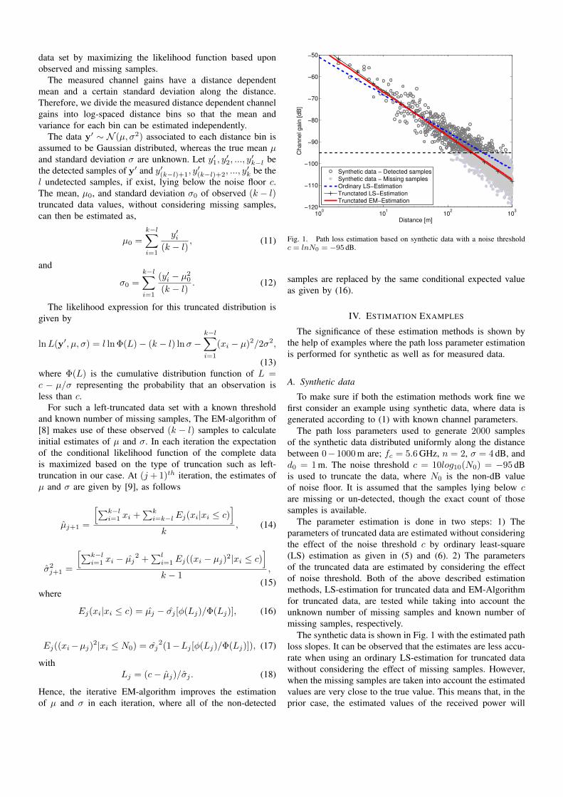
Fig. 1. Path loss estimation based on synthetic data with a noise thresholdc = lnN0 = −95 dB.
samples are replaced by the same conditional expected valueas given by (16).
IV. ESTIMATION EXAMPLES
The significance of these estimation methods is shown bythe help of examples where the path loss parameter estimationis performed for synthetic as well as for measured data.
A. Synthetic data
To make sure if both the estimation methods work fine wefirst consider an example using synthetic data, where data isgenerated according to (1) with known channel parameters.
The path loss parameters used to generate 2000 samplesof the synthetic data distributed uniformly along the distancebetween 0− 1000 m are; fc = 5.6 GHz, n = 2, σ = 4 dB, andd0 = 1 m. The noise threshold c = 10log10(N0) = −95 dBis used to truncate the data, where N0 is the non-dB valueof noise floor. It is assumed that the samples lying below care missing or un-detected, though the exact count of thosesamples is available.
The parameter estimation is done in two steps: 1) Theparameters of truncated data are estimated without consideringthe effect of the noise threshold c by ordinary least-square(LS) estimation as given in (5) and (6). 2) The parametersof the truncated data are estimated by considering the effectof noise threshold. Both of the above described estimationmethods, LS-estimation for truncated data and EM-Algorithmfor truncated data, are tested while taking into account theunknown number of missing samples and known number ofmissing samples, respectively.
The synthetic data is shown in Fig. 1 with the estimated pathloss slopes. It can be observed that the estimates are less accu-rate when using an ordinary LS-estimation for truncated datawithout considering the effect of missing samples. However,when the missing samples are taken into account the estimatedvalues are very close to the true value. This means that, in theprior case, the estimated values of the received power will
be larger than the true values. The path loss model based onincorrect parameter estimates can thus lead to erroneous resultswhen performing network simulations.
The true and estimated values are listed in Table I for eachof the above described parameter estimation methods. Thetable shows that, for this specific example, when estimation isperformed without considering the missing samples, n is over-estimated whereas the standard deviation is underestimated.However, when the effects of the noise floor or the number ofmissing samples are considered, then the estimation results arevery similar to the true values. For the synthetic data in thisexample, both the truncated LS-estimation and the truncatedEM-estimation methods have similar performance.
TABLE IPATH LOSS PARAMETER ESTIMATION FOR SYNTHETIC DATA
n PL0 [dB] σ [dB]
True values 2 47.4 4Ordinary LS-estimation 1.61 -53.5 3.46
Truncated LS-estimation 1.91 -48.8 3.86Truncted EM-estimation 2.0 -46.6 3.84
B. Measurement data
The measurement data used here is collected for vehicle-to-vehicle (V2V) communication channel characterization at5.6 GHz, for details see [10]. The path loss model parameterfor the measurement data are estimated in the same way as it isdone in Section IV-A. The measurement data for two differentsituation line-of-sight (LOS), when both the TX and RX hasvisual sight between them, and obstructed-LOS (OLOS), whena large object such as building, or another vehicle partly orcompletely obstruct the LOS between the TX and RX. Boththe situations are significantly different from each other andreceiver power in LOS is typically better than that in OLOS.These differences in the received power result in differentnumber of missing samples is both scenarios for a fixed noisethreshold c, i.e., more samples will be missing in OLOSsituation.
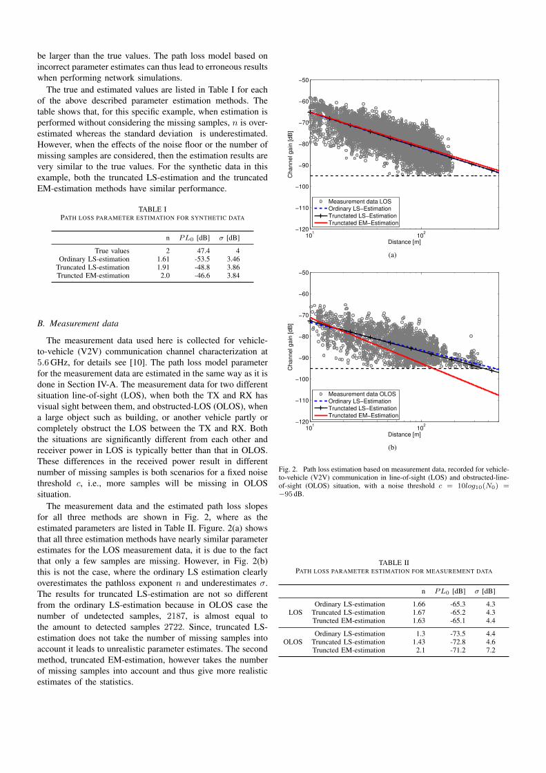
The measurement data and the estimated path loss slopesfor all three methods are shown in Fig. 2, where as theestimated parameters are listed in Table II. Figure. 2(a) showsthat all three estimation methods have nearly similar parameterestimates for the LOS measurement data, it is due to the factthat only a few samples are missing. However, in Fig. 2(b)this is not the case, where the ordinary LS estimation clearlyoverestimates the pathloss exponent n and underestimates σ.The results for truncated LS-estimation are not so differentfrom the ordinary LS-estimation because in OLOS case thenumber of undetected samples, 2187, is almost equal tothe amount to detected samples 2722. Since, truncated LS-estimation does not take the number of missing samples intoaccount it leads to unrealistic parameter estimates. The secondmethod, truncated EM-estimation, however takes the numberof missing samples into account and thus give more realisticestimates of the statistics.
101
102
−120
−110
−100
−90
−80
−70
−60
−50
Distance [m]
Ch
an
ne
l g
ain
[d
B]
Measurement data LOS
Ordinary LS−Estimation
Trunctated LS−Estimation
Trunctated EM−Estimation
(a)
101
102
−120
−110
−100
−90
−80
−70
−60
−50
Distance [m]
Ch
an
ne
l g
ain
[d
B]
Measurement data OLOS
Ordinary LS−Estimation
Trunctated LS−Estimation
Trunctated EM−Estimation
(b)
Fig. 2. Path loss estimation based on measurement data, recorded for vehicle-to-vehicle (V2V) communication in line-of-sight (LOS) and obstructed-line-of-sight (OLOS) situation, with a noise threshold c = 10log10(N0) =−95 dB.
TABLE IIPATH LOSS PARAMETER ESTIMATION FOR MEASUREMENT DATA
n PL0 [dB] σ [dB]
Ordinary LS-estimation 1.66 -65.3 4.3LOS Truncated LS-estimation 1.67 -65.2 4.3
Truncted EM-estimation 1.63 -65.1 4.4
Ordinary LS-estimation 1.3 -73.5 4.4OLOS Truncated LS-estimation 1.43 -72.8 4.6
Truncted EM-estimation 2.1 -71.2 7.2
V. SUMMARY AND CONCLUSIONS
In this paper, we present two novel ways of estimatingthe pathloss model parameters for the measurement data set,which is incomplete or truncated due to the influence of thenoise floor. We show that the estimates can be improved ifthe effects of the noise floor are taken into account in theestimation steps. In the truncated least-square (LS) estimationbased method, when the number of samples below the noisefloor is unknown, the noise floor is modeled with the help of atruncated normal distribution and the parameters are estimatedbased on a likelihood expression for this distribution. In thesecond method, when the number of samples above and belowthe noise floor is known, then both the noise floor informationas well as the number of samples below noise floor areused to estimate the model parameters using the expectationmaximization (EM) algorithm for truncated data. It is foundthat the EM-algorithm based method gives better estimatescompared to LS-estimation based method, given that a largenumber of samples are below the noise floor and that numberis known. When the number of samples below the noise flooris unknown, the trucated LS-estimation gives better parameterestimates than the ordinary LS method. All three methods givesimilar estimates when there are no samples below the noisefloor.
REFERENCES
[1] M. Hatay, “Empirical formula for propagation loss in land mobile radioservices,” Vehicular Technology, IEEE Transactions on, vol. 29, no. 3,pp. 317–325, Aug 1980.
[2] V. Erceg, L. Greenstein, S. Tjandra, S. Parkoff, A. Gupta, B. Kulic,A. Julius, and R. Bianchi, “An empirically based path loss modelfor wireless channels in suburban environments,” Selected Areas inCommunications, IEEE Journal on, vol. 17, no. 7, pp. 1205–1211, Jul1999.
[3] G. Mao, B. D. O. Anderson, and B. Fidan, “Wsn06-4: Online calibrationof path loss exponent in wireless sensor networks,” in Global Telecom-munications Conference, 2006. GLOBECOM ’06. IEEE, Nov 2006, pp.1–6.
[4] A. F. Molisch, F. Tufvesson, J. Karedal, and C. F. Mecklenbrauker, “Asurvey on vehicle-to-vehicle propagation channels,” in IEEE WirelessCommun. Mag., vol. 16, no. 6, 2009, pp. 12–22.
[5] J. Karedal, “Measurement-based modeling of wireless propagation chan-nels - MIMO and UWB,” Ph.D. dissertation, Department of Electricaland information technology, Lund University, Sweden, Feb. 2009.
[6] A. Molisch, Wireless Communications. Chichester, West Sussex, UK:IEEE Press-Wiley, 2005.
[7] L. Cheng, B. Henty, D. Stancil, F. Bai, and P. Mudalige, “Mobile vehicle-to-vehicle narrow-band channel measurement and characterization of the5.9 GHz dedicated short range communication (DSRC) frequency band,”Selected Areas in Communications, IEEE Journal on, vol. 25, no. 8, pp.1501 –1516, Oct. 2007.
[8] A. P. Dempster, N. M. Laird, and D. B. Rubin, “Maximum likelihoodfrom incomplete data via the em algorithm,” JOURNAL OF THE ROYALSTATISTICAL SOCIETY, SERIES B, vol. 39, no. 1, pp. 1–38, 1977.
[9] R. H. Shumway, A. S. Azari, and P. Johnson, “Estimating meanconcentrations under transformation for environmental data withdetection limits,” Technometrics, vol. 31, no. 3, pp. pp. 347–356, 1989.[Online]. Available: http://www.jstor.org/stable/3556144
[10] T. Abbas, F. Tufvesson, and J. Karedal, “Measurement based shadowfading model for vehicle-to-vehicle network simulations,” ArXiv e-prints,Mar. 2012.