ECONOMIC GROWTH CENTER

YALE UNIVERSITY

P.O. Box 208269New Haven, CT 06520-8269

http://www.econ.yale.edu/~egcenter/

CENTER DISCUSSION PAPER NO. 874

PATHS TO SUCCESS: THE RELATIONSHIP BETWEENHUMAN DEVELOPMENT AND ECONOMIC GROWTH

Michael BoozerYale University

Gustav RanisYale University

Frances StewartUniversity of Oxford

Tavneet SuriYale University

December 2003

Notes: Center Discussion Papers are preliminary materials circulated to stimulate discussions and criticalcomments.

We thank T.N. Srinivasan, T. Paul Schultz, and participants of the Yale Trade and Development seminarfor valuable comments.

Michael Boozer is at the Department of Economics and the Yale Center for International and Area Studies,Yale University. Gustav Ranis is Professor of International Economics and the Director of the Center forInternational and Area Studies, Yale University. Frances Stewart is Professor of Development Economicsand the Director of Queen Elizabeth House, University of Oxford. Tavneet Suri is at the Department ofEconomics, Yale University.

This paper can be downloaded without charge from the Social Science Research Network electroniclibrary at: http://ssrn.com/abstract=487469

An index to papers in the Economic Growth Center Discussion Paper Series is located at: http://www.econ.yale.edu/~egcenter/research.htm

Paths to Success: The Relationship Between HumanDevelopment and Economic Growth

Michael BoozerGustav Ranis

Frances StewartTavneet Suri

Abstract

This paper explores the two-way relationships between Economic Growth (EG) and HumanDevelopment (HD), building on an earlier work by Ranis, Stewart, and Ramirez (2000). Here,we show that HD is not only a product of EG but also an important input to it. The paperdevelops new empirical strategies to estimate the strength of the two-way chains connecting HDand EG. Building on existing growth literature, we explore the empirical determinants ofpositive growth trajectories running from HD to EG and find that HD plays an essential role inexplaining growth trajectories. Our findings point to the empirical relevance of endogenousgrowth models in general, and threshold effect models in particular. We also develop a measureof the strength of the EG to HD relationship and explore some of its empirical determinants. Astrong sequencing implication of our findings is that HD must be given priority for theachievement of both higher EG as well as HD.

Keyword: Human Development, Economic Growth, Threshold Models

JEL codes: O15, O57, C23

1 Introduction

Since Human Development (HD), which has been defined as enlarging people’s choices in a way which

enables them to lead longer, healthier and fuller lives, has come to the fore as a fundamental objective of

development3, its relationship to Economic Growth (EG) has become a central issue. This is not just a

matter of how the two relate at a particular point in time, but also addressed the question of sequencing

over time, which has major relevance to policy. This paper explores these two issues theoretically as well

as empirically. It takes off from previous work by Ranis, Stewart and Ramirez (2000) (henceforth RSR)

who provided an initial exploration of the two-way relationship between HD and EG.

There are two strands of the literature on economic development that are relevant here but have

tended to remain rather distinct. The predominant one has been concerned with the determinants of

EG, going back to classical times, extending to neo-classical growth models and, more recently, the “new

growth theory” models. The second strand asks what the ultimate objective of economic development

is and how to measure it, including a discussion of the determinants of HD. We take the position that

a long and healthy life represents the “bottom line” objective of human activity, even though this issue

continues to be contested.4

While both literatures have acknowledged the contribution of the other - e.g. human capital is

generally regarded as an important input into EG, and EG as providing the resources to achieve HD, the

cumulative intertemporal interaction between the two has been generally neglected. If HD is not only

an end product of the development process but also a means to generating future EG, the conventional

view of a uni-directional path is mis-specified. We contend that neither EG nor HD can be analyzed in

isolation of the other if one wants to understand how an economy got to its current state and where it

is going. This dual causation between HD and EG was first explored empirically by RSR. They defined

the loop connecting EG to HD and back again as two chains - Chain A running from EG to HD and

Chain B running from HD to EG. They also attempted to identify the main component links making up

3See Sen (1992) and Sugden (1993) for a statement and review of the issues in this debate. The Hu-

manDevelopment Reports of the UNDP present the Human Development Index (HDI) which is commonly

used to summarize some aspects of HD (health, education, etc.) into a scalar measure analogous to that

for EG.4For a brief introduction to this debate, see the papers by Srinivasan (1994), Aturupane, Glewwe, and

Isenman (1994), and Streeten (1994).

2

each chain and their relative strengths. Exploring country behavior over time, they also came to some

preliminary conclusions on the sequencing necessary for success in economic and human development.

This paper uses the analysis and findings of RSR as a point of departure to pull together the two liter-

atures mentioned above. It extends it in two major dimensions: first, it relates the two-way relationship

to contemporary growth theory; and, secondly, it develops empirical methods to assess the strengths of

the two chains mentioned above which helps illuminate the sequencing issue. We also discuss how contri-

butions to the endogenous growth literature, particularly those that focus on threshold externalities, can

explain both the long-run patterns observed by RSR between countries, as well as the time paths for EG

and HD within countries. Our empirical framework does not allow us to pinpoint a particular theoretical

structure among this class of models, but it illustrates the compatibility between the empirical work of

RSR on the sequencing priority of HD levels and threshold models that view aspects of HD as necessary

preconditions for the acceleration of EG.

The paper is structured as follows: in Section Two we review and update the evidence from RSR.

In Section Three we review the relevant theoretical development and growth literature. Section Four

develops a measure of the strength of Chain B, as represented by the growth trajectory for each country

and relates this to various measures of HD. Section Five presents a country-specific measure of the overall

strength of Chain A and explores its determinants. Section Six considers the interaction of the two chains

over time and explores the fundamental sequencing issue. Section Seven concludes.

2 Summary and Update of Previous Findings

We first review and update the evidence and concepts in RSR on which this paper builds. We interpret

HD as consisting of the health, nutrition and education levels of the population. Figure 1 provides the

schematic diagram of the various links in Chain A that connects EG to HD and Chain B that connects

HD to EG. Chain A shows how GDP is allocated to governments and households and how these agents

in turn decide how much of their resources are spent on items that are likely to promote HD, such as

basic education, water, food, primary health care, etc. It also includes resources allocated by households

or governments to NGOs promoting HD. While EG is thus an important element in improving HD,

the relationship is not automatic but depends on the distribution of income and the propensities of

3

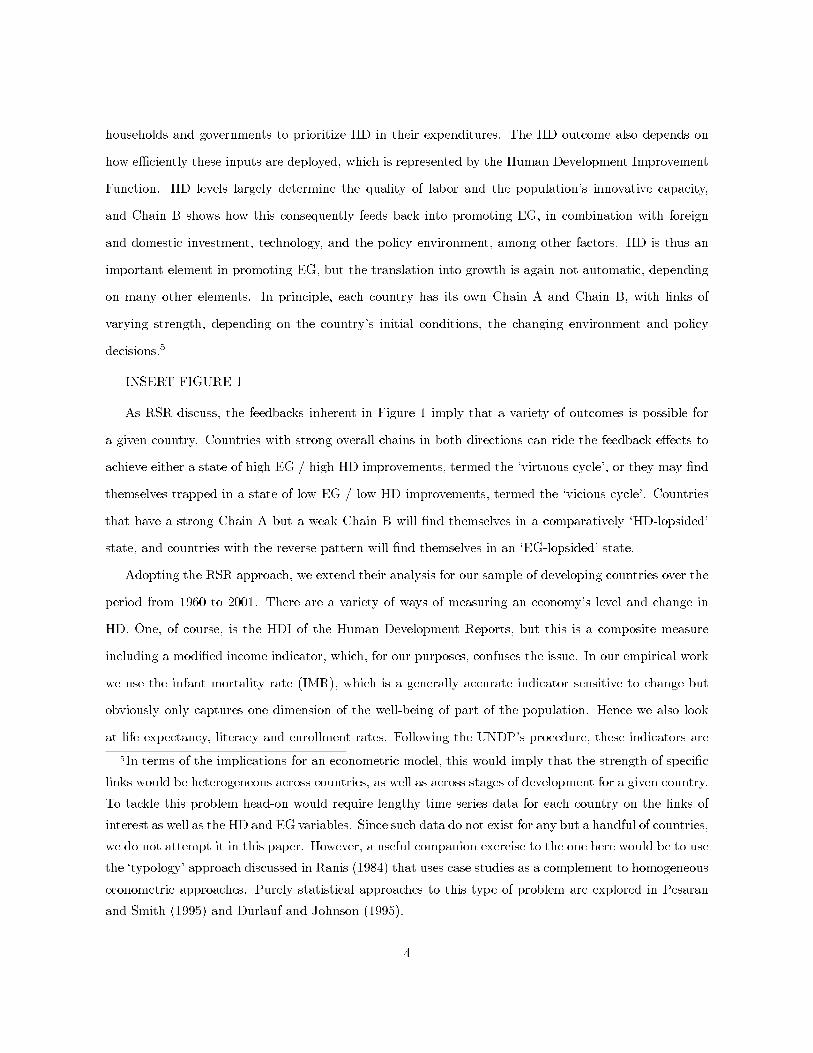
households and governments to prioritize HD in their expenditures. The HD outcome also depends on

how efficiently these inputs are deployed, which is represented by the Human Development Improvement

Function. HD levels largely determine the quality of labor and the population’s innovative capacity,

and Chain B shows how this consequently feeds back into promoting EG, in combination with foreign

and domestic investment, technology, and the policy environment, among other factors. HD is thus an

important element in promoting EG, but the translation into growth is again not automatic, depending

on many other elements. In principle, each country has its own Chain A and Chain B, with links of

varying strength, depending on the country’s initial conditions, the changing environment and policy

decisions.5

INSERT FIGURE 1

As RSR discuss, the feedbacks inherent in Figure 1 imply that a variety of outcomes is possible for

a given country. Countries with strong overall chains in both directions can ride the feedback effects to

achieve either a state of high EG / high HD improvements, termed the ‘virtuous cycle’, or they may find

themselves trapped in a state of low EG / low HD improvements, termed the ‘vicious cycle’. Countries

that have a strong Chain A but a weak Chain B will find themselves in a comparatively ‘HD-lopsided’

state, and countries with the reverse pattern will find themselves in an ‘EG-lopsided’ state.

Adopting the RSR approach, we extend their analysis for our sample of developing countries over the

period from 1960 to 2001. There are a variety of ways of measuring an economy’s level and change in

HD. One, of course, is the HDI of the Human Development Reports, but this is a composite measure

including a modified income indicator, which, for our purposes, confuses the issue. In our empirical work

we use the infant mortality rate (IMR), which is a generally accurate indicator sensitive to change but

obviously only captures one dimension of the well-being of part of the population. Hence we also look

at life expectancy, literacy and enrollment rates. Following the UNDP’s procedure, these indicators are

5In terms of the implications for an econometric model, this would imply that the strength of specific

links would be heterogeneous across countries, as well as across stages of development for a given country.

To tackle this problem head-on would require lengthy time series data for each country on the links of

interest as well as the HD and EG variables. Since such data do not exist for any but a handful of countries,

we do not attempt it in this paper. However, a useful companion exercise to the one here would be to use

the ‘typology’ approach discussed in Ranis (1984) that uses case studies as a complement to homogeneous

econometric approaches. Purely statistical approaches to this type of problem are explored in Pesaran

and Smith (1995) and Durlauf and Johnson (1995).

4

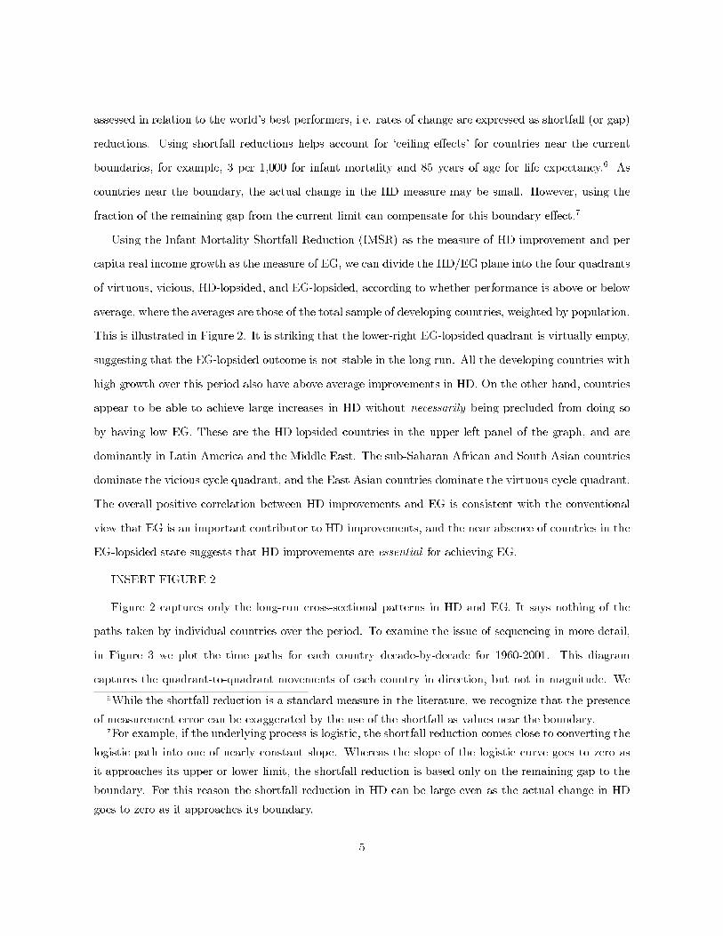
assessed in relation to the world’s best performers, i.e. rates of change are expressed as shortfall (or gap)

reductions. Using shortfall reductions helps account for ‘ceiling effects’ for countries near the current

boundaries, for example, 3 per 1,000 for infant mortality and 85 years of age for life expectancy.6 As

countries near the boundary, the actual change in the HD measure may be small. However, using the

fraction of the remaining gap from the current limit can compensate for this boundary effect.7

Using the Infant Mortality Shortfall Reduction (IMSR) as the measure of HD improvement and per

capita real income growth as the measure of EG, we can divide the HD/EG plane into the four quadrants

of virtuous, vicious, HD-lopsided, and EG-lopsided, according to whether performance is above or below

average, where the averages are those of the total sample of developing countries, weighted by population.

This is illustrated in Figure 2. It is striking that the lower-right EG-lopsided quadrant is virtually empty,

suggesting that the EG-lopsided outcome is not stable in the long run. All the developing countries with

high growth over this period also have above average improvements in HD. On the other hand, countries

appear to be able to achieve large increases in HD without necessarily being precluded from doing so

by having low EG. These are the HD-lopsided countries in the upper-left panel of the graph, and are

dominantly in Latin America and the Middle East. The sub-Saharan African and South Asian countries

dominate the vicious cycle quadrant, and the East Asian countries dominate the virtuous cycle quadrant.

The overall positive correlation between HD improvements and EG is consistent with the conventional

view that EG is an important contributor to HD improvements, and the near absence of countries in the

EG-lopsided state suggests that HD improvements are essential for achieving EG.

INSERT FIGURE 2

Figure 2 captures only the long-run cross-sectional patterns in HD and EG. It says nothing of the

paths taken by individual countries over the period. To examine the issue of sequencing in more detail,

in Figure 3 we plot the time paths for each country decade-by-decade for 1960-2001. This diagram

captures the quadrant-to-quadrant movements of each country in direction, but not in magnitude. We

6While the shortfall reduction is a standard measure in the literature, we recognize that the presence

of measurement error can be exaggerated by the use of the shortfall as values near the boundary.7For example, if the underlying process is logistic, the shortfall reduction comes close to converting the

logistic path into one of nearly constant slope. Whereas the slope of the logistic curve goes to zero as

it approaches its upper or lower limit, the shortfall reduction is based only on the remaining gap to the

boundary. For this reason the shortfall reduction in HD can be large even as the actual change in HD

goes to zero as it approaches its boundary.

5

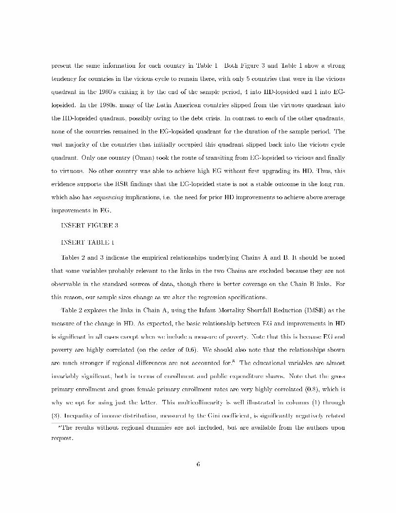
present the same information for each country in Table 1. Both Figure 3 and Table 1 show a strong

tendency for countries in the vicious cycle to remain there, with only 5 countries that were in the vicious

quadrant in the 1960’s exiting it by the end of the sample period, 4 into HD-lopsided and 1 into EG-

lopsided. In the 1980s, many of the Latin American countries slipped from the virtuous quadrant into

the HD-lopsided quadrant, possibly owing to the debt crisis. In contrast to each of the other quadrants,

none of the countries remained in the EG-lopsided quadrant for the duration of the sample period. The

vast majority of the countries that initially occupied this quadrant slipped back into the vicious cycle

quadrant. Only one country (Oman) took the route of transiting from EG-lopsided to vicious and finally

to virtuous. No other country was able to achieve high EG without first upgrading its HD. Thus, this

evidence supports the RSR findings that the EG-lopsided state is not a stable outcome in the long run,

which also has sequencing implications, i.e. the need for prior HD improvements to achieve above average

improvements in EG.

INSERT FIGURE 3

INSERT TABLE 1

Tables 2 and 3 indicate the empirical relationships underlying Chains A and B. It should be noted

that some variables probably relevant to the links in the two Chains are excluded because they are not

observable in the standard sources of data, though there is better coverage on the Chain B links. For

this reason, our sample sizes change as we alter the regression specifications.

Table 2 explores the links in Chain A, using the Infant Mortality Shortfall Reduction (IMSR) as the

measure of the change in HD. As expected, the basic relationship between EG and improvements in HD

is significant in all cases except when we include a measure of poverty. Note that this is because EG and

poverty are highly correlated (on the order of 0.6). We should also note that the relationships shown

are much stronger if regional differences are not accounted for.8 The educational variables are almost

invariably significant, both in terms of enrollment and public expenditure shares. Note that the gross

primary enrollment and gross female primary enrollment rates are very highly correlated (0.8), which is

why we opt for using just the latter. This multicollinearity is well illustrated in columns (1) through

(3). Inequality of income distribution, measured by the Gini coefficient, is significantly negatively related

8The results without regional dummies are not included, but are available from the authors upon

request.

6

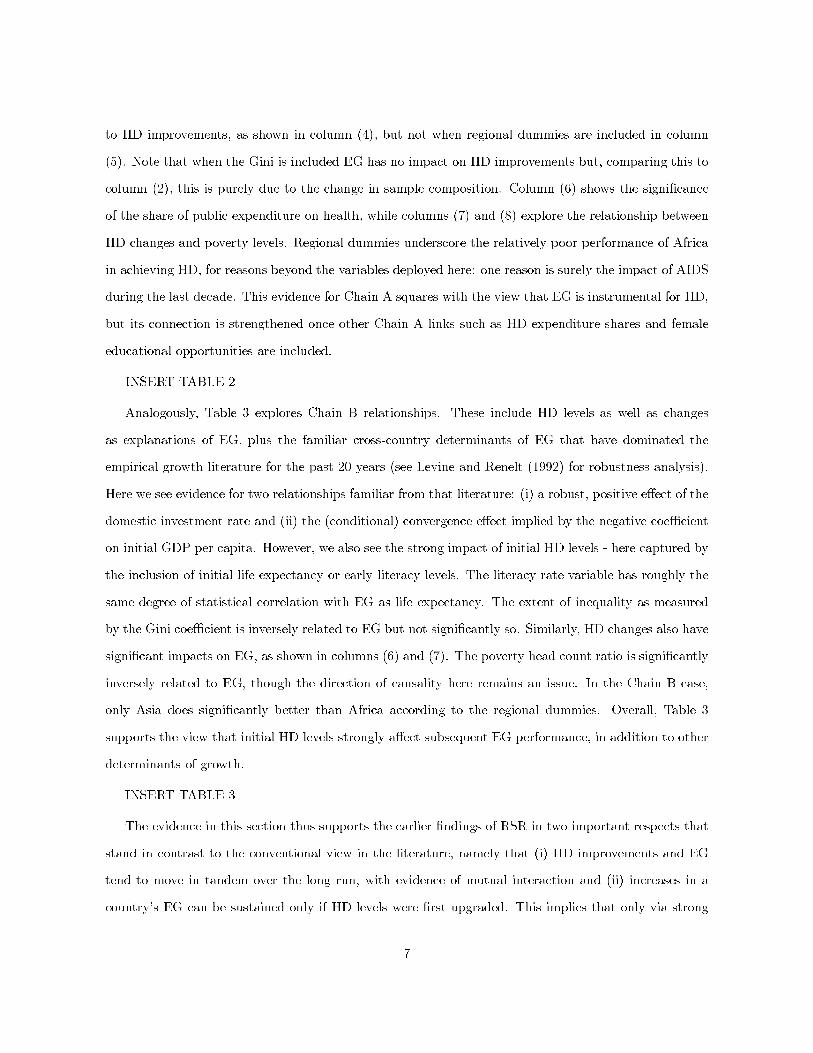
to HD improvements, as shown in column (4), but not when regional dummies are included in column

(5). Note that when the Gini is included EG has no impact on HD improvements but, comparing this to

column (2), this is purely due to the change in sample composition. Column (6) shows the significance

of the share of public expenditure on health, while columns (7) and (8) explore the relationship between

HD changes and poverty levels. Regional dummies underscore the relatively poor performance of Africa

in achieving HD, for reasons beyond the variables deployed here: one reason is surely the impact of AIDS

during the last decade. This evidence for Chain A squares with the view that EG is instrumental for HD,

but its connection is strengthened once other Chain A links such as HD expenditure shares and female

educational opportunities are included.

INSERT TABLE 2

Analogously, Table 3 explores Chain B relationships. These include HD levels as well as changes

as explanations of EG, plus the familiar cross-country determinants of EG that have dominated the

empirical growth literature for the past 20 years (see Levine and Renelt (1992) for robustness analysis).

Here we see evidence for two relationships familiar from that literature: (i) a robust, positive effect of the

domestic investment rate and (ii) the (conditional) convergence effect implied by the negative coefficient

on initial GDP per capita. However, we also see the strong impact of initial HD levels - here captured by

the inclusion of initial life expectancy or early literacy levels. The literacy rate variable has roughly the

same degree of statistical correlation with EG as life expectancy. The extent of inequality as measured

by the Gini coefficient is inversely related to EG but not significantly so. Similarly, HD changes also have

significant impacts on EG, as shown in columns (6) and (7). The poverty head count ratio is significantly

inversely related to EG, though the direction of causality here remains an issue. In the Chain B case,

only Asia does significantly better than Africa according to the regional dummies. Overall, Table 3

supports the view that initial HD levels strongly affect subsequent EG performance, in addition to other

determinants of growth.

INSERT TABLE 3

The evidence in this section thus supports the earlier findings of RSR in two important respects that

stand in contrast to the conventional view in the literature, namely that (i) HD improvements and EG

tend to move in tandem over the long run, with evidence of mutual interaction and (ii) increases in a

country’s EG can be sustained only if HD levels were first upgraded. This implies that only via strong

7

HD can the virtuous cycle be attained. Direct attempts to strengthen EG without first enhancing HD

can, at best, lead to temporary increases in EG, with a relapse into a vicious cycle. This contradicts the

neoclassical view that inputs into the growth process are always substitutable. It also contrasts with the

conventional view that perceives HD more as a product of growth than as an input. Figures 3 and Table

1 indicate the need for a framework that will permit us to examine the sequencing issue more precisely.

This will require us to explore what is needed for a particular country to move from a vicious to a virtuous

cycle over time.

3 Growth Paths, Threshold Effects, and Human Development

This section discusses briefly the relevant literature on human development and economic growth and the

relationship of this paper to that literature. As mentioned earlier, our work is relevant to two literatures,

one to the debate regarding the ultimate objective of economic activity and the role of EG in achieving

it, and the second to the determinants of EG. These two literatures have generally remained separate.

This section clearly illustrates the links between the two and how the views of these two literatures on

the roles of HD and EG relate to our empirical analysis.

Much of the literature on HD has focused on what the appropriate measures of economic development

are and whether EG or per capita income levels are sufficient as measures of the well-being of a population.

While it is generally accepted that EG provides the means by which an economy can upgrade its HD

levels, the HD literature questions whether EG is sufficient as a measure of development. There is no

doubt that EG expands a country’s choice set, but the issue still remains of how to assess the ultimate

objective of economic development.9 This debate has overshadowed a careful analysis of the linkages

joining HD and EG. For the most part, the HD literature specifies a unidirectional path from EG into

improved HD outcomes. But, if HD is not only an end-product of the development process, but also a

means to future EG, then such a unidirectional view leads to a mis-specification of the relationship.

In comparison, the literature on EG is vast. While, until recently, much of it has followed the

neoclassical growth model of Solow (1956), the notion that HD is not just an outcome of the EG allocation

process but serves as an input as well, is not new. From Lewis (1955) to more recent work on endogenous

9See Sen (1992) and Sugden (1993) for more detail on this debate.

8

growth theory, human capital has been given a significant role in the determination of EG, in terms of

education, health and nutrition.

In his discussion of prioritizing educational expenditures, Lewis (1955) acknowledges that “the dif-

ficulty that education raises is that it is both a consumer and an investment service”. Bowman and

Anderson (1963) try to disentangle the future productivity role of education from its current consump-

tion role empirically by analyzing various leads and lags of education measures and national income. They

also provide some of the first evidence that the payoff to literacy may exhibit threshold effects dependent

on the fraction of an economy that is literate. Uzawa (1965) considers a broader view of HD where he

takes the factor multiplying the production function, A, as reproducible and no longer ‘exogenous’ as

in the neoclassical model. Whereas later authors such as Romer (1986, 1990) narrowed their definition

of A to be R&D, ‘ideas’, etc., Uzawa’s initial model was more in line with our paper by viewing A as

the “various activities in the form of education, health, construction and maintenance of public goods,

etc., which result in an improvement of labor efficiency”. This framework was later modified by Lucas

(1988) who instead assumed a linear production technology for A, in which case growth rates need not

go to zero in finite time. Lucas’ reflections on the alternative sources of sustained growth from 1960 era

models showed how countries could grow at different rates indefinitely, depending on their human capital.

Whether it was the changes or the stocks of human capital depended on the precise mechanism used to

model the endogenous growth process.

The analysis of this paper is certainly compatible with the overall message of the endogenous growth

literature. However, the majority of these models fail to capture some fundamental elements of our

empirical work. One flaw is that the literature often models elements of HD more as consumption goods

rather than as causal factors determining future growth. This is simply a modeling issue, in that including

HD both as cause and as a result of EG leads to ill-behaved (e.g. unbounded) dynamic properties of the

equilibrium paths unless sufficient restrictions are placed on the model parameters. This is not a serious

shortcoming of the theoretical models per se, but it is a problem for the empirical work to disentangle

causation from association. A far more serious shortcoming of the Uzawa-Lucas type endogenous growth

models is that they cannot account for the non-linearities in the growth paths that we saw in Figure

3. Lucas (1988) considered models which could explain permanent differences in growth rates across

countries. Such models account for purely cross-sectional patterns, like those in Figure 2. But this class

9

of endogenous growth models cannot explain how a given country can go from a low-EG state to a high-

EG state over time. To model this phenomenon we need to turn to the class of threshold-externality

models as proposed by Azariadis and Drazen (1990). Their model is similar to the Lucas framework,

except that around the ‘critical mass’ threshold for a given level of education, the other inputs are not

smoothly substitutable for education. A minimum level of education must therefore be attained before

an economy can escape from a low-level development trap - analogous to the vicious cycle of RSR. Thus,

while the Uzawa-Lucas models focus on explaining purely cross-sectional differences in growth rates,

Azariadis and Drazen go a step further to explain permanent shifts in growth rates within countries.

Note that the Azariadis-Drazen framework is not entirely ‘new’. Like its contemporary counterpart,

Murphy, Shleifer, and Vishny (1989), it is a version of the ‘Big Push’ ideas of Rosenstein-Rodan (1943)

and Nurkse (1953) who note that an economy can remain stuck in an underdeveloped state unless there is

a coordinated large investment effort. Hirschman (1958) critiqued this ‘balanced growth’ view by arguing

that the unbalancing across sectors of an economy is what pulls or pushes an economy upward and Rostow

(1960) suggested distinct stages of economic growth, but focused more on the univariate characteristics of

EG as opposed to the identifying causes and mechanisms of what was responsible for moving the economy

from one stage to the next. Since the Azariadis and Drazen paper explores long-run changes in trends

of EG and how it interacts with HD, their framework is clearly appropriate for our analysis, the more so

since the threshold nature of the model explains why HD is not smoothly substitutable for other inputs

as it is in more conventional growth models. Moreover, the empirical work in both this paper and RSR

offer an identifiable channel, HD, by which an economy can move from a vicious to a virtuous cycle.10

Since these threshold models are most relevant to our empirical work, the question arises as to whether

such thresholds have been detected empirically. Perron (1989) and Andrews (1993) provide the statistical

tools to test for trend breaks in a given time series. In principle, such univariate tests could detect the

threshold externality and link the change point to underlying causal factors such as HD. Alternatively,

if we had a precise formulation of the country-specific dynamics linking HD and EG, we could estimate

a series of country-specific VARs linking HD and EG. However, the time series dimension of the data

used in this paper is far too limited to allow either of these two approaches to be feasible.11 The

10Galor and Weil (2000) develop a related model for the quantity and quality of children, and a dynamic

interrelation between human capital and technological progress.11However, time series data on individual countries or select groups of countries may be lengthy enough

10

empirical approach we outline below does not formulate such precise dynamic relationships, but instead

acknowledges that there is an underlying, country-specific, dynamic relationship that summarize by its

key parameters.

The overall message from this brief survey of related literature is that, while human development

has long been viewed both as an input and an outcome of the development process, the feedback and

dual causality between HD and EG has not been fully or empirically taken into account. Once this dual

causality is taken into account, it is obvious that any analysis of the determinants of EG or HD alone

is incomplete. A feedback loop like that shown in Figure 1 implies that neither EG nor HD can be

analyzed in isolation of the other if one wants to understand how an economy got to its current state and

where it is going. The endogenous growth models allow for an explanation of cross-sectional differences

in the growth experiences of countries, but Figure 1 requires models of the threshold externality type to

understand changes over time within a given economy. This paper analyzes the latter, by allowing the

strength of the feedback effects to vary by country.

4 Growth Paths: Measuring the Strength of Links in Chain B

In order to explore the relationship between HD and country growth over time, we require a measure

for each country which captures the trend change in growth, which we shall term its ’growth trajectory’.

The most common version of the time path of EG used in the empirical growth literature is the average

growth in per capita income over an entire sample period (e.g. Barro and Sala-i-Martin (1992)), which

has the virtue of averaging out short run fluctuations in growth, thus allowing the analyst to focus on

explaining differences in country patterns of long run growth.12 However, for our purposes, this measure

to allow such an approach in limited cases. Wallack (2003) is a recent example of this approach for

Indian data from 1951 to 2001. Crafts (1995) and Crafts and Mills (1996) used this approach to study

the growth path of British industrial production from 1700 to 1900. Jones (1995) used OECD data to

argue that there has been no break in the trend of GDP per capita, yet innovative activity increased

greatly over his sample period.12This is not always the case. Islam (1995) uses fixed effects analysis in his study of convergence, thereby

removing the purely cross-sectional variation in growth rates, and focusing on short run fluctuations in

growth. Our strategy retains the virtue of Islam’s approach by allowing for cross-country heterogeneity,

but also keeps the focus on long run trends, thus by-passing one of the central criticisms of his approach.

11

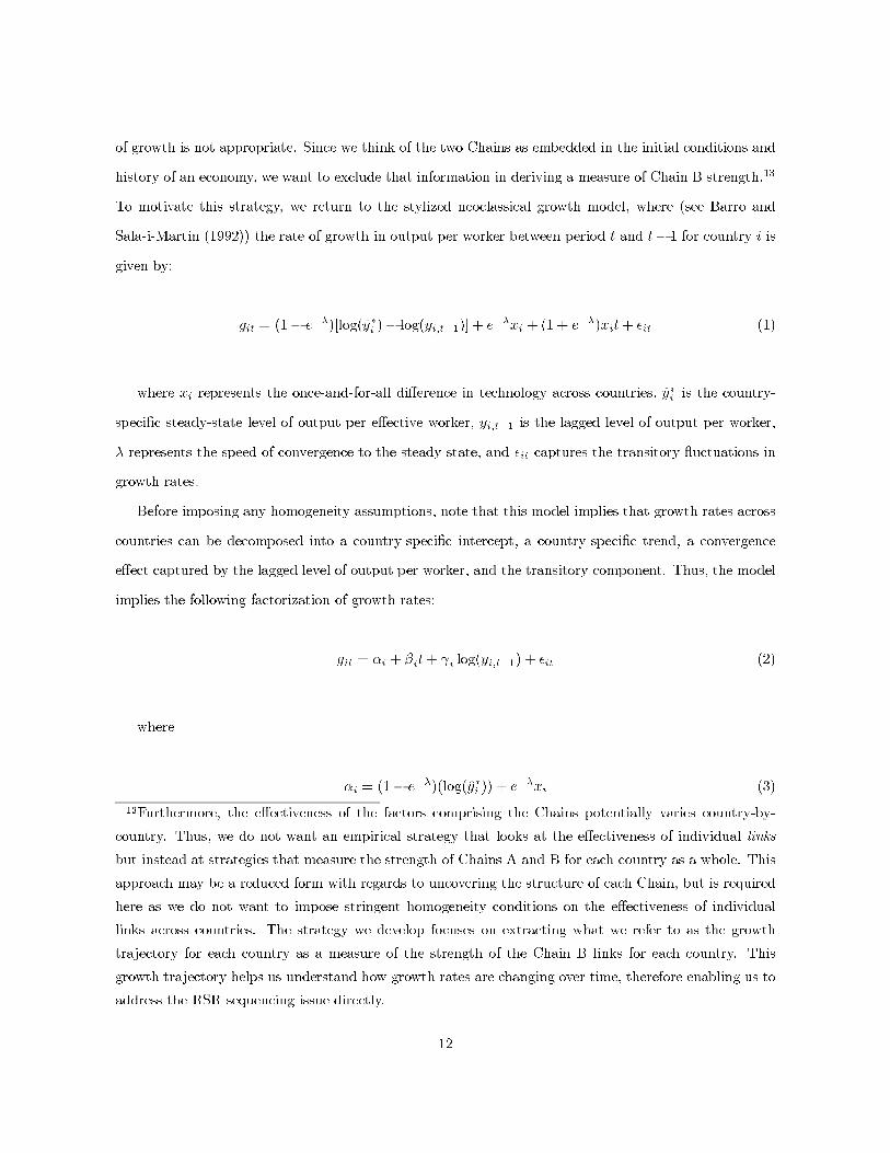
of growth is not appropriate. Since we think of the two Chains as embedded in the initial conditions and

history of an economy, we want to exclude that information in deriving a measure of Chain B strength.13

To motivate this strategy, we return to the stylized neoclassical growth model, where (see Barro and

Sala-i-Martin (1992)) the rate of growth in output per worker between period t and t− 1 for country i is

given by:

git = (1− e−λ)[log(y∗i )− log(yi,t−1)] + e−λxi + (1 + e−λ)xit+ εit (1)

where xi represents the once-and-for-all difference in technology across countries, y∗i is the country-

specific steady-state level of output per effective worker, yi,t−1 is the lagged level of output per worker,

λ represents the speed of convergence to the steady state, and εit captures the transitory fluctuations in

growth rates.

Before imposing any homogeneity assumptions, note that this model implies that growth rates across

countries can be decomposed into a country-specific intercept, a country-specific trend, a convergence

effect captured by the lagged level of output per worker, and the transitory component. Thus, the model

implies the following factorization of growth rates:

git = αi + βit+ γi log(yi,t−1) + εit (2)

where

αi = (1− e−λ)(log(y∗i )) + e−λxi (3)

13Furthermore, the effectiveness of the factors comprising the Chains potentially varies country-by-

country. Thus, we do not want an empirical strategy that looks at the effectiveness of individual links

but instead at strategies that measure the strength of Chains A and B for each country as a whole. This

approach may be a reduced form with regards to uncovering the structure of each Chain, but is required

here as we do not want to impose stringent homogeneity conditions on the effectiveness of individual

links across countries. The strategy we develop focuses on extracting what we refer to as the growth

trajectory for each country as a measure of the strength of the Chain B links for each country. This

growth trajectory helps us understand how growth rates are changing over time, therefore enabling us to

address the RSR sequencing issue directly.

12

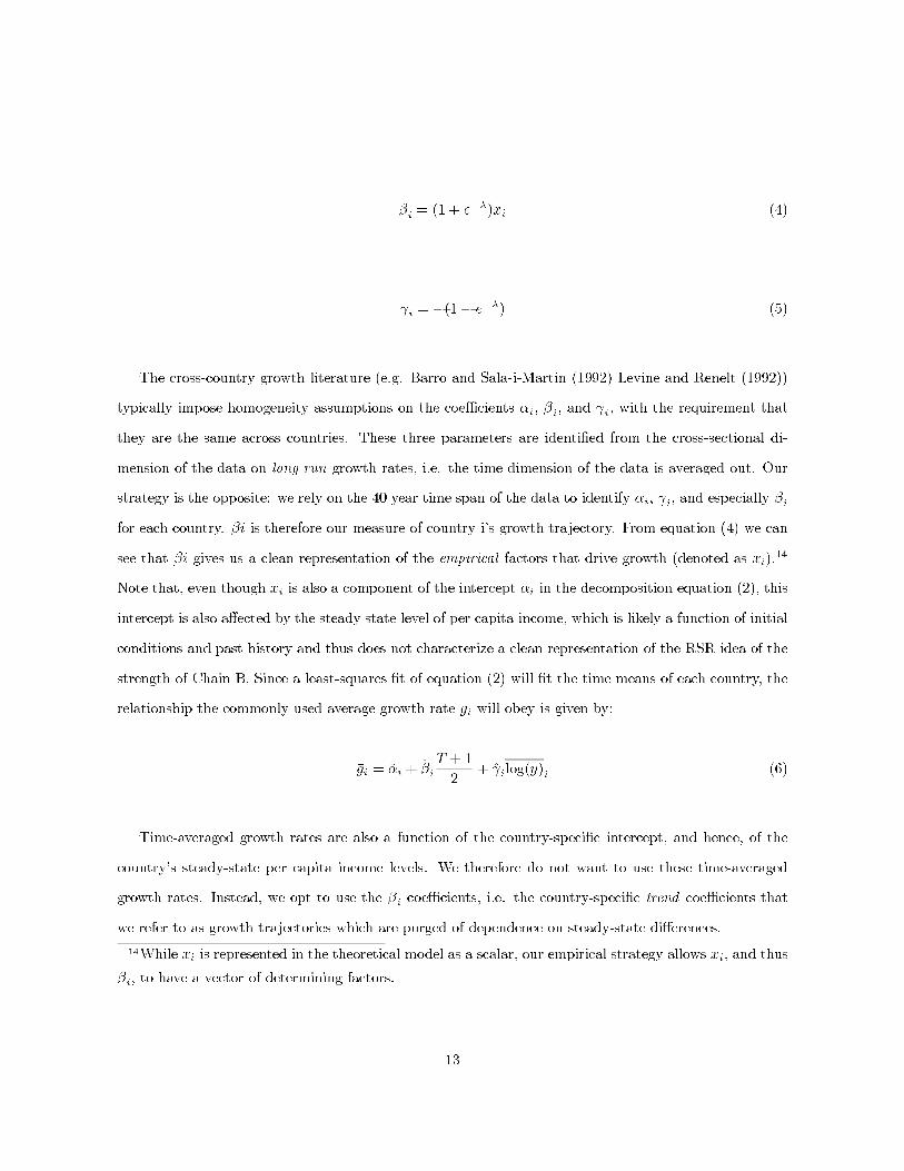
βi= (1 + e−λ)xi (4)

γi= −(1− e−λ) (5)

The cross-country growth literature (e.g. Barro and Sala-i-Martin (1992) Levine and Renelt (1992))

typically impose homogeneity assumptions on the coefficients αi, βi, and γ

i, with the requirement that

they are the same across countries. These three parameters are identified from the cross-sectional di-

mension of the data on long run growth rates, i.e. the time dimension of the data is averaged out. Our

strategy is the opposite: we rely on the 40 year time span of the data to identify αi, γi, and especially βi

for each country. βi is therefore our measure of country i’s growth trajectory. From equation (4) we can

see that βi gives us a clean representation of the empirical factors that drive growth (denoted as xi).14

Note that, even though xi is also a component of the intercept αi in the decomposition equation (2), this

intercept is also affected by the steady state level of per capita income, which is likely a function of initial

conditions and past history and thus does not characterize a clean representation of the RSR idea of the

strength of Chain B. Since a least-squares fit of equation (2) will fit the time means of each country, the

relationship the commonly used average growth rate gi will obey is given by:

gi = αi + βi

T + 1

2+ γ

ilog(y)

i(6)

Time-averaged growth rates are also a function of the country-specific intercept, and hence, of the

country’s steady-state per capita income levels. We therefore do not want to use these time-averaged

growth rates. Instead, we opt to use the βicoefficients, i.e. the country-specific trend coefficients that

we refer to as growth trajectories which are purged of dependence on steady-state differences.

14While xi is represented in the theoretical model as a scalar, our empirical strategy allows xi, and thus

βi, to have a vector of determining factors.

13

Note that our empirical approach is broader than this neoclassical theoretical foundation. The decom-

position of growth rates in (2) is compatible with a large number of neoclassical and endogenous/threshold

growth models, even though we relied on the Solow model to derive it. In the neoclassical formulation

there are only the once-and-for-all factors summarized in xi that explain trend differences across coun-

tries. Endogenous growth models of the Uzawa-Lucas variety also explain permanent differences in growth

trends but endogenize xi, the source of permanent growth. Hence both exogenous and endogenous sources

of growth will be captured by the trend coefficients in our estimates of equation (2), country-by-country.

The question that then arises is how useful are the estimates obtained from equation (2) if the growth

path is non-linear? In fact, we saw in the evidence presented above (Figure 3), that growth paths are

often non-linear. In principle, we could use the 40 year time span of EG to fit a non-linear trend specific to

each country. However, detecting trend breaks when using annual observations is not feasible in practice.

If it were, we could potentially distinguish the threshold externality models that imply that differences

in trend growth occur only across rather than within countries. Moreover, the linear trend will still be

a good summary of the growth trajectory even if the underlying trend is non-linear, since our trajectory

coefficient βibroadly indicates whether the path of EG is increasing, flat, or decreasing over the 40 year

time span of our sample.

We obtain a measure of βiby applying OLS to equation (2), for each country.15 This process generates

15An issue arises in the estimation of the equation in terms of which per capita income series to use.

Due to the presence of lagged income level as a regressor, whether we use a nominal or real series has a

significant impact on the results, with the nominal series leading to much more variation in the βiseries.

Since the regressions are country-specific, we do not need to convert per capita incomes to PPP or world

prices. Problems with using PPP estimates, including the pricing of non-traded goods and services, and

biases due to relative price shifts have been discussed by Bhagwati and Hansen (1973), Nuxoll (1994)

and Srinivasan (1995). Our procedure for estimating the βicoefficients therefore involves using current

per capita series on growth and income. But we need to allow for inflation since the data is all in current

prices. We pre-filter all the per capita income series of region, time, and region-by-time effects (remember

that we use the lagged level of per capita incomes in estimating the βicoefficients). We also pre-filter

the growth rates of time effects as world growth rates tend to have a certain trend over time and we

would like to account for that. We then use the filtered growth rates and lagged per capita levels in

the country-by-country estimation of equation (3). Use of the raw series preserves more of the variation

and gives stronger results than those presented here but we want to avoid results driven by potentially

nominal effects.

14

the country-specific growth trajectories, βi, which essentially are the average rate of change of the growth

rate and that we take to be a measure of the strength of Chain B. Keep in mind that a country can have

a positive growth trajectory, with βi> 0, yet have negative average growth, gi < 0. All but 10 countries

have growth trajectories within the range of -0.2 to 0.2 - βi≈ 0, i.e. actual growth rates that are neither

increasing nor decreasing. Average growth rates over the period, by contrast, vary much more widely

across countries. Barro (1997) and Quah (1996) note that the time-series movements in per capita output

are a trivial fraction of the cross-country variation in levels of output per capita. Having derived our

measure of the growth trajectory, the next step is to ask what its empirical determinants are, particularly

its relationship to levels and changes in HD.

The evidence on sequencing presented in Figure 3 and Table 1 above led us to hypothesize that HD

levels and/or improvements affect countries’ growth trajectories. We therefore investigate the relationship

between HD levels, HD changes, and βi. This relationship is an indication of the strength of Chain B. We

also explore the role of more conventional explanatory factors of EG (as in Levine and Renelt (1992)),

such as investment and export ratios, in determining the growth trajectory. However, since such factors

are generally associated with actual growth rates, we would anticipate that only their changes would

explain the growth trajectory, βi. We specify our empirical model as follows:

βi= η +HD′

iτ + z′

iθ + ζ

i(7)

where i = 1, . . . ,81, the number of countries for which we have data; and z′

irepresents the other

factors influencing βinoted above, as well as three regional dummies. The presence of the error term ζ

i

highlights another advantage of our two-step estimation procedure in that it allows for heterogeneity in

the Chain B measure for reasons that are not purely due to HD. Our focus is on the estimated value(s) of

the coefficient vector τ , as we hypothesize that higher levels of HD lead to higher (more positive) growth

trajectories, and vice versa. While specific theoretical models dictate whether the variables should be

entered in the form of levels or changes, we treat this as an empirical issue and consider a variety of

specifications.16 Since HD is a product of EG, via Chain A, in order to reduce the problem of reverse

16The extended neoclassical framework of Mankiw, Romer, and Weil (1992) implies that stocks or levels

of HD drive growth. However, Benhabib and Spiegel (1994) find that HD levels explain little of EG itself,

but that the human capital stock interacted with the diffusion of innovations (as in the analysis of Nelson

15

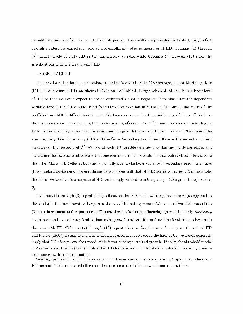
causality we use data from early in the sample period. The results are presented in Table 4, using infant

mortality rates, life expectancy and school enrollment rates as measures of HD. Columns (1) through

(6) include levels of early HD as the explanatory variable while Columns (7) through (12) show the

specifications with changes in early HD.

INSERT TABLE 4

The results of the basic specification, using the ‘early’ (1960 to 1980 average) Infant Mortality Rate

(IMR) as a measure of HD, are shown in Column 1 of Table 4. Larger values of IMR indicate a lower level

of HD, so that we would expect to see an estimated τ that is negative. Note that since the dependent

variable here is the fitted time trend from the decomposition in equation (2), the actual value of the

coefficient on IMR is difficult to interpret. We focus on comparing the relative size of the coefficients on

the regressors, as well as observing their statistical significance. From Column 1, we can see that a higher

IMR implies a country is less likely to have a positive growth trajectory. In Columns 2 and 3 we repeat the

exercise, using Life Expectancy (LE) and the Gross Secondary Enrollment Rate as the second and third

measures of HD, respectively.17 We look at each HD variable separately as they are highly correlated and

measuring their separate influence within one regression is not possible. The schooling effect is less precise

than the IMR and LE effects, but this is partially due to the lower variance in secondary enrollment rates

(the standard deviation of the enrollment rate is about half that of IMR across countries). On the whole,

the initial levels of various aspects of HD are strongly related to subsequent positive growth trajectories,

βi.

Columns (4) through (6) repeat the specifications for HD, but now using the changes (as opposed to

the levels) in the investment and export ratios as additional regressors. We can see from Columns (1) to

(3) that investment and exports are still operative mechanisms influencing growth, but only increasing

investment and export rates lead to increasing growth trajectories, and not the levels themselves, as is

the case with HD. Columns (7) through (12) repeat the exercise, but now focusing on the role of HD

and Phelps (1966)) is significant. The endogenous growth models along the lines of Uzawa-Lucas generally

imply that HD changes are the reproducible factor driving sustained growth. Finally, the threshold model

of Azariadis and Drazen (1990) implies that HD levels govern the threshold at which an economy transits

from one growth trend to another.17Average primary enrollment rates vary much less across countries and tend to ‘top out’ at values over

100 percent. Their estimated effects are less precise and reliable so we do not report them.

16

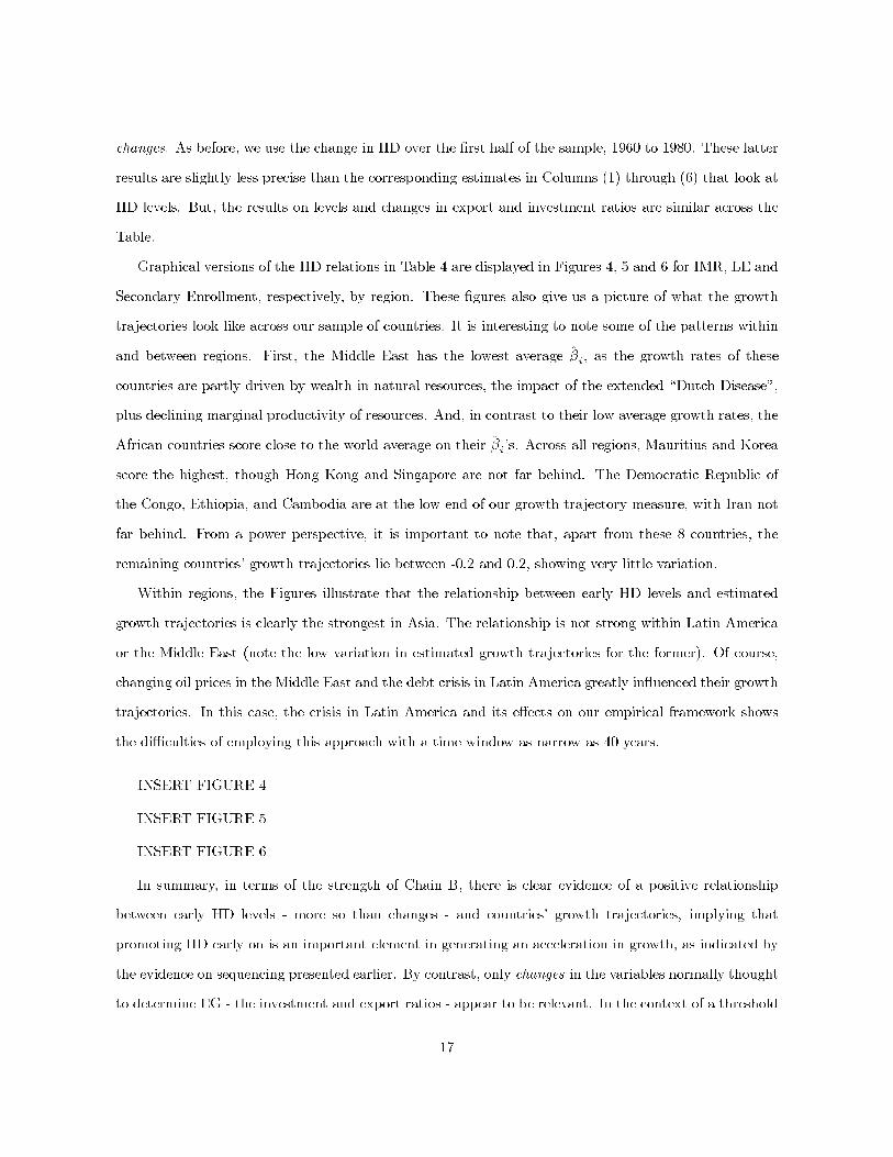
changes. As before, we use the change in HD over the first half of the sample, 1960 to 1980. These latter

results are slightly less precise than the corresponding estimates in Columns (1) through (6) that look at

HD levels. But, the results on levels and changes in export and investment ratios are similar across the

Table.

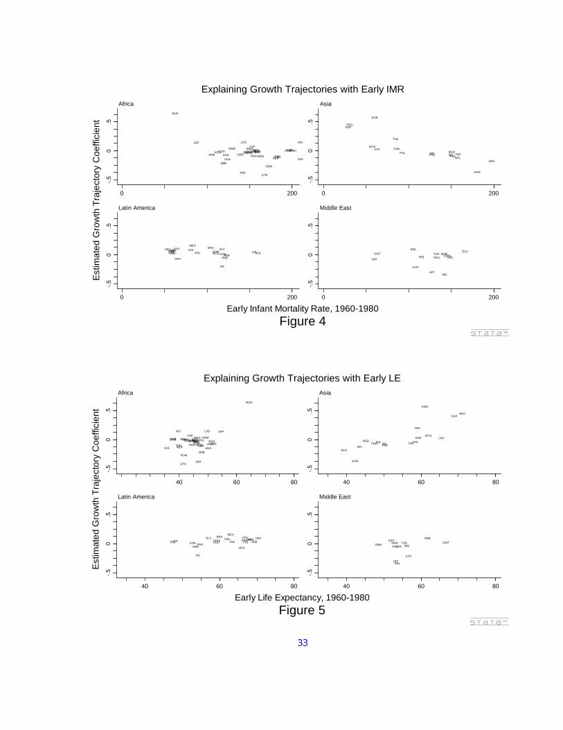
Graphical versions of the HD relations in Table 4 are displayed in Figures 4, 5 and 6 for IMR, LE and

Secondary Enrollment, respectively, by region. These figures also give us a picture of what the growth

trajectories look like across our sample of countries. It is interesting to note some of the patterns within

and between regions. First, the Middle East has the lowest average βi, as the growth rates of these

countries are partly driven by wealth in natural resources, the impact of the extended “Dutch Disease”,

plus declining marginal productivity of resources. And, in contrast to their low average growth rates, the

African countries score close to the world average on their βi’s. Across all regions, Mauritius and Korea

score the highest, though Hong Kong and Singapore are not far behind. The Democratic Republic of

the Congo, Ethiopia, and Cambodia are at the low end of our growth trajectory measure, with Iran not

far behind. From a power perspective, it is important to note that, apart from these 8 countries, the

remaining countries’ growth trajectories lie between -0.2 and 0.2, showing very little variation.

Within regions, the Figures illustrate that the relationship between early HD levels and estimated

growth trajectories is clearly the strongest in Asia. The relationship is not strong within Latin America

or the Middle East (note the low variation in estimated growth trajectories for the former). Of course,

changing oil prices in the Middle East and the debt crisis in Latin America greatly influenced their growth

trajectories. In this case, the crisis in Latin America and its effects on our empirical framework shows

the difficulties of employing this approach with a time window as narrow as 40 years.

INSERT FIGURE 4

INSERT FIGURE 5

INSERT FIGURE 6

In summary, in terms of the strength of Chain B, there is clear evidence of a positive relationship

between early HD levels - more so than changes - and countries’ growth trajectories, implying that

promoting HD early on is an important element in generating an acceleration in growth, as indicated by

the evidence on sequencing presented earlier. By contrast, only changes in the variables normally thought

to determine EG - the investment and export ratios - appear to be relevant. In the context of a threshold

17

externality model, if we interpret the threshold as a country-specific level of HD, the results in Table 4

lend such a model strong support. These results indeed also show weak support for a model without such

‘pre-conditions’, as in an Uzawa-Lucas type model where HD is simply an input to production. However,

they provide stronger evidence for the view that HD is non-substitutable, but must reach some threshold

level before the transition is made from a low level to a high level equilibrium. Determining a specific

threshold level of HD that is a necessary prerequisite for achieving accelerating growth would, however,

go beyond the scope of this paper.

5 From GDP to Human Development : Measuring the Strength

of the Links in Chain A

In the case of Chain A, data availability, over time, is more limited than in the case of Chain B, permit-

ting less investigation of country-specific heterogeneity. Moreover, theoretical and conceptual models to

account for what generates HD improvements are not as developed as those explaining EG. In construct-

ing an overall measure of the strength of Chain A, we therefore are forced to rely on the cross-sectional

relationship between EG and HD improvements to generate a country-specific measure. We use the lags

inherent in enhancing HD levels from higher EG to reduce the problem of reverse causality.

In order to construct a measure of the overall strength of Chain A for each country, we use country-

specific fitted residuals from a regression of ‘late’ (1980-2000) HD improvements on ‘early’ EG (1960-1980).

The idea is that, given initial growth, countries that have better HD at the end of the sample period (i.e.

higher fitted residuals) are inferred to have been more effective in translating EG into HD, presumably

because they have invested more of the profits of initial growth into developing their HD infrastructure,

and hence have stronger links in Chain A. To formalize our measurement strategy, let the early and late

halves of our sample be represented by the 0 and 1 subscripts, respectively, so that, in principle, we can

use the following equation to estimate the country-specific strengths of Chain A:

∆HDi1 = κ +ψigi0 + ξ

i(8)

18

where the country-specific conversion of dollars of early growth into HD is given by the country-specific

slope ψi. Unfortunately, this regression has only 80 observations, but 81 parameters, to estimate if the

slope parameters are allowed to be heterogeneous. If we wished to pursue this strategy, we could try to

push the time series dimension to its limits and extract 2 or 3 time periods per country, but in so doing

we would have to make much more precise assumptions on the lag structure in the above model. While,

in principle, this approach is roughly consistent with our Chain B approach discussed above, in practice

the smaller number of time series points makes this far too imprecise to be a viable strategy.

Instead, we turn to the cross-sectional relationship between ∆HDi1 and gi0 and ask: for a given early

growth gi0, what is the later improvement in HD? The answer to this question is simply the fitted residual

to the homogeneous slope coefficient regression:

∆HDi1 = κ+ ψgi0 + vi (9)

Call this fitted residual vi. Note that by the mechanics of OLS, this measure is independent of gi0,

and note further that interpreting this measure of the strength of Chain A when compared to the slope

measure above implies that:

vi = ξi+ (ψ

i−ψ)gi0 (10)

If the regression error, ξi, is small , i.e. if a necessary condition for HD improvement is growth in

income, EG, which represents the view that EG is ‘instrumental’ for HD, then this cross-section-based

method using the fitted residuals will largely reflect the efficiency of converting early EG into later HD

improvements. Thus vi will serve as a suitable measure of the strength of the links in Chain A, given a

particular measure of HD.

To construct a measure of the relative overall strength of Chain A for each country, therefore, we use

the country-specific residuals from a regression of HD improvements, 1980 to 2000, on EG, from 1960 to

1980. This measure of Chain A strength is thus independent of early EG by construction, and yet we find

that it has a strong positive correlation with growth at the end of the sample period. Here again, the lag

time in producing HD reduces the possibility of simultaneity driving this clear, positive relationship.

19

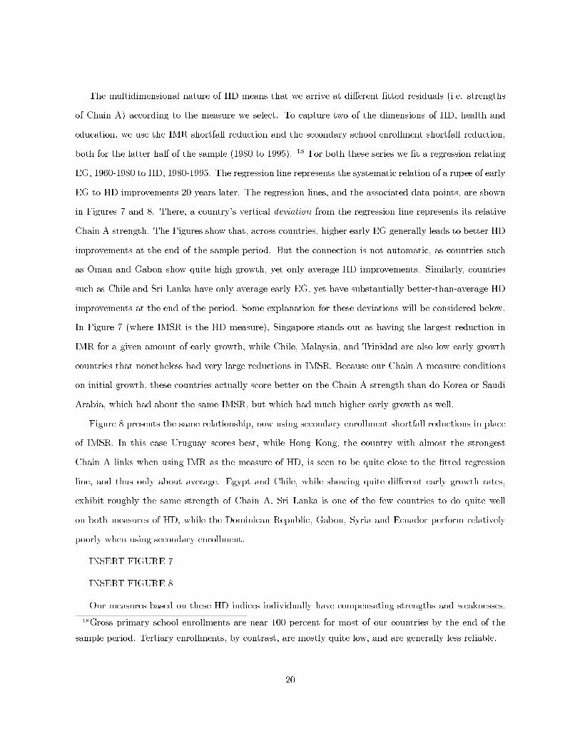
The multidimensional nature of HD means that we arrive at different fitted residuals (i.e. strengths

of Chain A) according to the measure we select. To capture two of the dimensions of HD, health and

education, we use the IMR shortfall reduction and the secondary school enrollment shortfall reduction,

both for the latter half of the sample (1980 to 1995). 18 For both these series we fit a regression relating

EG, 1960-1980 to HD, 1980-1995. The regression line represents the systematic relation of a rupee of early

EG to HD improvements 20 years later. The regression lines, and the associated data points, are shown

in Figures 7 and 8. There, a country’s vertical deviation from the regression line represents its relative

Chain A strength. The Figures show that, across countries, higher early EG generally leads to better HD

improvements at the end of the sample period. But the connection is not automatic, as countries such

as Oman and Gabon show quite high growth, yet only average HD improvements. Similarly, countries

such as Chile and Sri Lanka have only average early EG, yet have substantially better-than-average HD

improvements at the end of the period. Some explanation for these deviations will be considered below.

In Figure 7 (where IMSR is the HD measure), Singapore stands out as having the largest reduction in

IMR for a given amount of early growth, while Chile, Malaysia, and Trinidad are also low early growth

countries that nonetheless had very large reductions in IMSR. Because our Chain A measure conditions

on initial growth, these countries actually score better on the Chain A strength than do Korea or Saudi

Arabia, which had about the same IMSR, but which had much higher early growth as well.

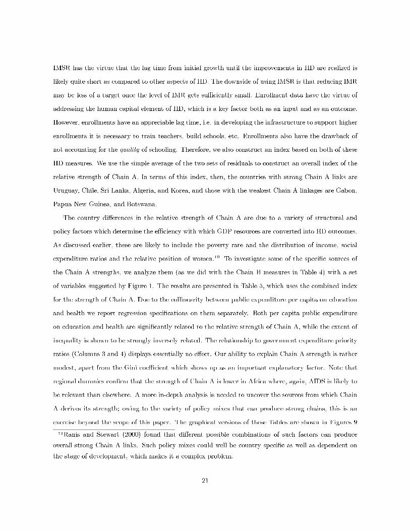
Figure 8 presents the same relationship, now using secondary enrollment shortfall reductions in place

of IMSR. In this case Uruguay scores best, while Hong Kong, the country with almost the strongest

Chain A links when using IMR as the measure of HD, is seen to be quite close to the fitted regression

line, and thus only about average. Egypt and Chile, while showing quite different early growth rates,

exhibit roughly the same strength of Chain A. Sri Lanka is one of the few countries to do quite well

on both measures of HD, while the Dominican Republic, Gabon, Syria and Ecuador perform relatively

poorly when using secondary enrollment.

INSERT FIGURE 7

INSERT FIGURE 8

Our measures based on these HD indices individually have compensating strengths and weaknesses.

18Gross primary school enrollments are near 100 percent for most of our countries by the end of the

sample period. Tertiary enrollments, by contrast, are mostly quite low, and are generally less reliable.

20

IMSR has the virtue that the lag time from initial growth until the improvements in HD are realized is

likely quite short as compared to other aspects of HD. The downside of using IMSR is that reducing IMR

may be less of a target once the level of IMR gets sufficiently small. Enrollment data have the virtue of

addressing the human capital element of HD, which is a key factor both as an input and as an outcome.

However, enrollments have an appreciable lag time, i.e. in developing the infrastructure to support higher

enrollments it is necessary to train teachers, build schools, etc. Enrollments also have the drawback of

not accounting for the quality of schooling. Therefore, we also construct an index based on both of these

HD measures. We use the simple average of the two sets of residuals to construct an overall index of the

relative strength of Chain A. In terms of this index, then, the countries with strong Chain A links are

Uruguay, Chile, Sri Lanka, Algeria, and Korea, and those with the weakest Chain A linkages are Gabon,

Papua New Guinea, and Botswana.

The country differences in the relative strength of Chain A are due to a variety of structural and

policy factors which determine the efficiency with which GDP resources are converted into HD outcomes.

As discussed earlier, these are likely to include the poverty rate and the distribution of income, social

expenditure ratios and the relative position of women.19 To investigate some of the specific sources of

the Chain A strengths, we analyze them (as we did with the Chain B measures in Table 4) with a set

of variables suggested by Figure 1. The results are presented in Table 5, which uses the combined index

for the strength of Chain A. Due to the collinearity between public expenditure per capita on education

and health we report regression specifications on them separately. Both per capita public expenditure

on education and health are significantly related to the relative strength of Chain A, while the extent of

inequality is shown to be strongly inversely related. The relationship to government expenditure priority

ratios (Columns 3 and 4) displays essentially no effect. Our ability to explain Chain A strength is rather

modest, apart from the Gini coefficient which shows up as an important explanatory factor. Note that

regional dummies confirm that the strength of Chain A is lower in Africa where, again, AIDS is likely to

be relevant than elsewhere. A more in-depth analysis is needed to uncover the sources from which Chain

A derives its strength; owing to the variety of policy mixes that can produce strong chains, this is an

exercise beyond the scope of this paper. The graphical versions of these Tables are shown in Figures 9

19Ranis and Stewart (2000) found that different possible combinations of such factors can produce

overall strong Chain A links. Such policy mixes could well be country specific as well as dependent on

the stage of development, which makes it a complex problem.

21

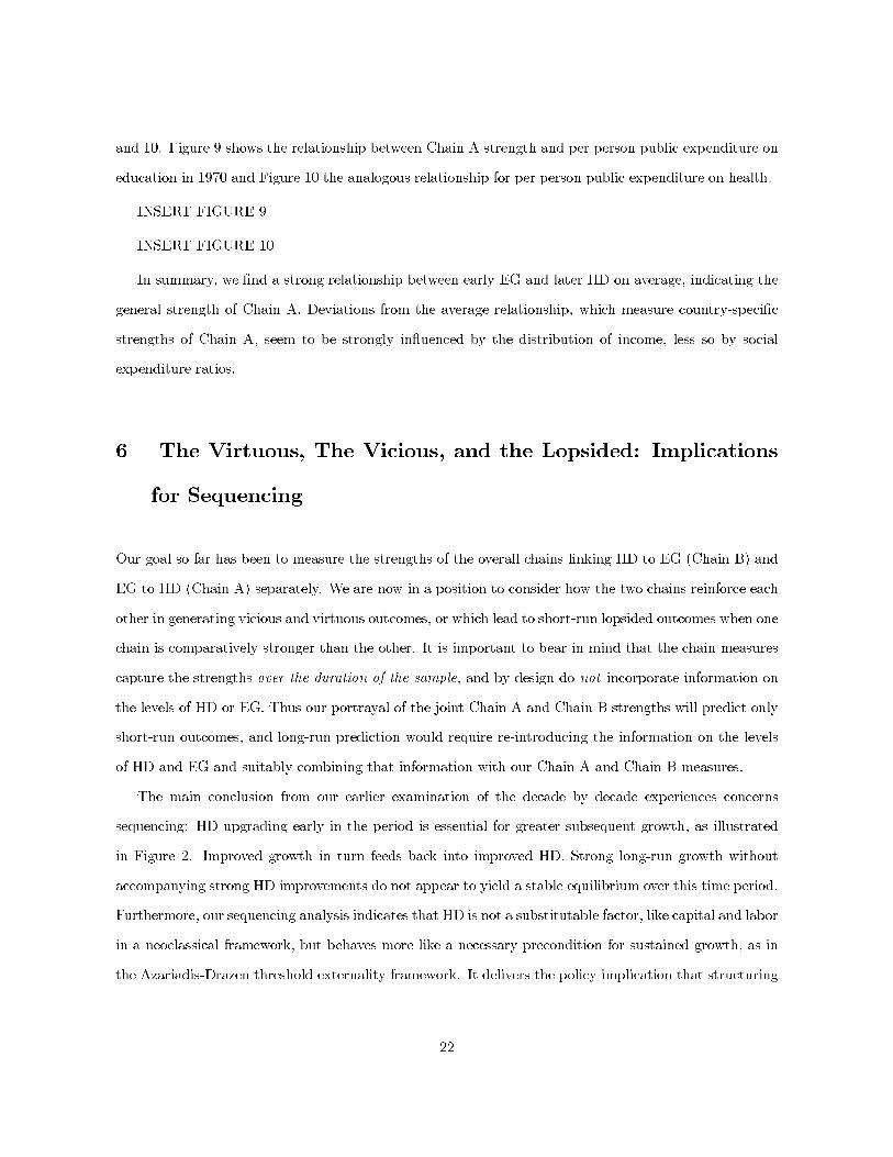
and 10. Figure 9 shows the relationship between Chain A strength and per person public expenditure on

education in 1970 and Figure 10 the analogous relationship for per person public expenditure on health.

INSERT FIGURE 9

INSERT FIGURE 10

In summary, we find a strong relationship between early EG and later HD on average, indicating the

general strength of Chain A. Deviations from the average relationship, which measure country-specific

strengths of Chain A, seem to be strongly influenced by the distribution of income, less so by social

expenditure ratios.

6 The Virtuous, The Vicious, and the Lopsided: Implications

for Sequencing

Our goal so far has been to measure the strengths of the overall chains linking HD to EG (Chain B) and

EG to HD (Chain A) separately. We are now in a position to consider how the two chains reinforce each

other in generating vicious and virtuous outcomes, or which lead to short-run lopsided outcomes when one

chain is comparatively stronger than the other. It is important to bear in mind that the chain measures

capture the strengths over the duration of the sample, and by design do not incorporate information on

the levels of HD or EG. Thus our portrayal of the joint Chain A and Chain B strengths will predict only

short-run outcomes, and long-run prediction would require re-introducing the information on the levels

of HD and EG and suitably combining that information with our Chain A and Chain B measures.

The main conclusion from our earlier examination of the decade by decade experiences concerns

sequencing: HD upgrading early in the period is essential for greater subsequent growth, as illustrated

in Figure 2. Improved growth in turn feeds back into improved HD. Strong long-run growth without

accompanying strong HD improvements do not appear to yield a stable equilibrium over this time period.

Furthermore, our sequencing analysis indicates that HD is not a substitutable factor, like capital and labor

in a neoclassical framework, but behaves more like a necessary precondition for sustained growth, as in

the Azariadis-Drazen threshold externality framework. It delivers the policy implication that structuring

22

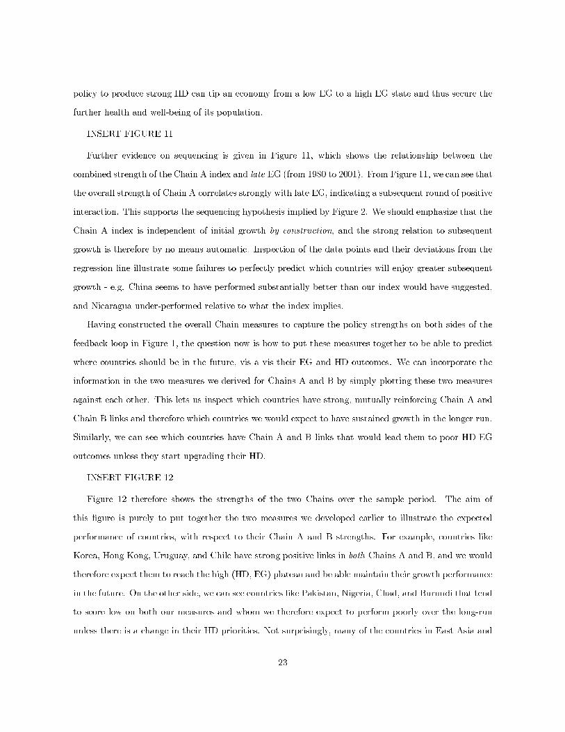
policy to produce strong HD can tip an economy from a low EG to a high EG state and thus secure the

further health and well-being of its population.

INSERT FIGURE 11

Further evidence on sequencing is given in Figure 11, which shows the relationship between the

combined strength of the Chain A index and late EG (from 1980 to 2001). From Figure 11, we can see that

the overall strength of Chain A correlates strongly with late EG, indicating a subsequent round of positive

interaction. This supports the sequencing hypothesis implied by Figure 2. We should emphasize that the

Chain A index is independent of initial growth by construction, and the strong relation to subsequent

growth is therefore by no means automatic. Inspection of the data points and their deviations from the

regression line illustrate some failures to perfectly predict which countries will enjoy greater subsequent

growth - e.g. China seems to have performed substantially better than our index would have suggested,

and Nicaragua under-performed relative to what the index implies.

Having constructed the overall Chain measures to capture the policy strengths on both sides of the

feedback loop in Figure 1, the question now is how to put these measures together to be able to predict

where countries should be in the future, vis a vis their EG and HD outcomes. We can incorporate the

information in the two measures we derived for Chains A and B by simply plotting these two measures

against each other. This lets us inspect which countries have strong, mutually reinforcing Chain A and

Chain B links and therefore which countries we would expect to have sustained growth in the longer run.

Similarly, we can see which countries have Chain A and B links that would lead them to poor HD-EG

outcomes unless they start upgrading their HD.

INSERT FIGURE 12

Figure 12 therefore shows the strengths of the two Chains over the sample period. The aim of

this figure is purely to put together the two measures we developed earlier to illustrate the expected

performance of countries, with respect to their Chain A and B strengths. For example, countries like

Korea, Hong Kong, Uruguay, and Chile have strong positive links in both Chains A and B, and we would

therefore expect them to reach the high (HD, EG) plateau and be able maintain their growth performance

in the future. On the other side, we can see countries like Pakistan, Nigeria, Chad, and Burundi that tend

to score low on both our measures and whom we therefore expect to perform poorly over the long-run

unless there is a change in their HD priorities. Not surprisingly, many of the countries in East Asia and

23

Latin America have strong linkages in both chains. Indeed, outside of these two regions only Tunisia and

Egypt in the Middle East, and Sri Lanka in South Asia are countries that we estimate to have strong

dual linkages that would tend to push them to the virtuous (HD-EG) plateau.

Finally, we comment on the over-representation of countries in the EG lopsided quadrant. As we

discussed above, our chain measures by construction discarded information on levels. However, the

threshold model of Azariadis and Drazen and the empirical analysis of RSR is predicated on HD levels.

As our analysis is constructed to abstract from initial conditions and thus the levels of HD, Figure 12

should not be expected to mimic the realized outcomes given in Figure 2. Were we to combine the rankings

on the HD levels with the predicted outcomes in Figure 12, this would push the few African countries

in the EG-lopsided into the vicious quadrant, consistent with their actual experience. Alternatively we

view the ‘predictions’ of Figure 12 as alludng to the future paths of the countries in the sample, and

the comparative strengths and weaknesses of their Chains A and B. As a strong Chain B without an

accompanying strong Chain A implies that high EG is not sustainable, we would expect the countries in

the lower right-hand quadrant to experience high EG for a temporary period at best. Figure 12 thus

identifies a number of countries with EG-centric policy mixes that would be well served, in terms of long

run growth and human development, by giving priority to enhancing their HD infrastructures.

7 Conclusion

The aim of this paper has been to understand the two-way linkages between HD and EG, accounting

for the fact that HD is likely to be not just an end product of growth, but an input as well and a key

ingredient in the development process. Education, health, and other aspects of HD involve fixed costs

that can create non-convexities in the social returns to various levels of HD, and thus result in low and

high level equilibria. This paper is concerned with how to measure the strength of the overall chains

linking EG to HD, following earlier evidence by Ranis, Stewart, and Ramirez (2000).

In Section 2 we updated the relationships identified by RSR, relating HD and EG cross-country over

time, using average growth as our measure of EG and absolute levels and changes in several definitions

of HD. In Sections 3 and 4, we presented more sophisticated measures of EG and HD and used these

to explore their interrelationship. In this case our aim was to explore individual country EG and HD

24

performance. In the case of EG, we developed the notion of country growth trajectories which basically

are defined as the trend change in growth in each country. In the case of HD, the relative strength

of Chain A for each country was defined by the deviations from the overall cross-country relationship

between early average economic growth and later improvements in HD.

While there are evident positive relationships between HD and EG, they are not automatic in either

direction. This paper has explored some of the factors explaining why some countries have particularly

strong Chains. In the case of Chain A, our investigations suggest that social expenditure ratios and

income distribution are important contributory factors. In the case of Chain B, it is the levels and

changes in HD and changes in investment ratios that are important contributing factors to the growth

trajectory. Of course, in both cases this omits other factors that are often emphasized, such as the quality

of the social services, and the prevalence of social capital in the case of A, and geography, institutions

and the policy environment in the case of B.20 We also showed how HD improvements must precede

growth-oriented policies if growth is to be sustained. These sequencing and level effects of HD contradict

the usual neoclassical view whereby all inputs to production are substitutable. The sequencing finding

also contradicts the conventional view that HD is purely a result of, as opposed to being a critical input

into long run expansions in EG.

The findings of long-run differences in growth paths, not only across countries but also within a given

country over time, restrict the class of theoretical models that can explain such phenomena. Endogenous

growth models of the Uzawa (1965) and Lucas (1988) type only explain long run differences in growth

across countries when they have differing propensities to upgrade HD. In contrast, threshold externality

models along the lines of Azariadis and Drazen (1990) were constructed precisely to explain the type of

phenomenon found in this paper, i.e. why transitions from a vicious (low EG low HD) state to a virtuous

(mutually re-enforcing high EG high HD) state over time are blocked unless HD is sufficiently strong

before EG centered policies are attempted.

20See North (1990), Sachs (2001) and Acemoglu, Johnson and Robinson (2002).

25

References

[1] Acemoglu, Daron, S. Johnson, and James Robinson, (2002), “Reversal of Fortune: Geography in

the Institutions in the Making of the Modern World Income Distribution”, Quarterly Journal of

Economics, CXVII, 1231-94.

[2] Aghion, Philippe and Peter Howitt, (1998), Endogenous Growth Theory, MIT Press, 1998.

[3] Andrews, Donald, W.K., (1993), “Tests for Parameter Instability and Structural Change with Un-

known Change Point”, Econometrica, 61(4), 821-856.

[4] Aturupane, Harsha, Paul Glewwe and Paul Isenman, (1994), “Poverty, Human Development and

Growth: An Emerging Consensus?”, American Economic Review, Papers and Proceedings, 84(2),

244-249.

[5] Azariadis, Costas, and Alan Drazen, (1990), “Threshold Externalities in Economic Development”,

The Quarterly Journal of Economics, 105(2), 501-526.

[6] Barro, Robert, (1997), Determinants of Economic Growth: A Cross-Country Empirical Study, Lionel

Robbins Lectures, MIT Press.

[7] Barro, Robert and Xavier Sala-i-Martin, (1995), Economic Growth, Advanced Series in Economics,

McGraw-Hill.

[8] Barro, Robert and Xavier Sala-i-Martin, (1992), “Convergence”, Journal of Political Economy,

100(2), 223-251.

[9] Benhabib, Jess, and Mark M. Spiegel, (1994), “The Role of Human Capital in Economic Develop-

ment: Evidence from Cross-Country Data”, Journal of Monetary Economics, 34, 143-173.

[10] Bowman, Mary Jean and C. Arnold Anderson, (1963), “Concerning the Role of Education in Devel-

opment”, in Clifford Geertz ed. Old Societies and New States, New York: Free Press, 247-279.

[11] Crafts, Nicholas, (1995), “Exogenous or Endogenous Growth? The Industrial Revolution Reconsid-

ered,” The Journal of Economic History 55(4), 745-772.

26

[12] Durlauf, Steven and Danny Quah (1999), “The New Empirics of Economic Growth”, in Taylor, John

and Michael Woodford, eds., Handbook of Macroeconomics, Volume 1A, Elsevier Science, North-

Holland, 235-308.

[13] Durlauf, Stephen and Johnson, (1995), “Multiple Regimes and Cross-Country Growth Behaviior”,

Journal of Applie Econometrics, 10, 365- 384.

[14] Hirshman, Albert, O., (1958), The Strategy of Economic Development, New Haven, Yale University

Press.

[15] Kakwani, Nanak, (1997), “Growth Rates of Per-Capita Income and Aggregate Welfare: An Interna-

tional Comparison”, The Review of Economics and Statistics, 79(2), 201-211.

[16] Kuznets, Simon, (1963), “Notes on The Take-off,” in W. W. Rostow ed. The Economics of Take-off

Into Sustain Growth, London: St. Martin’s Press.

[17] Levine, Ross and David Renelt, (1992), “A Sensitivity Analysis of Cross-Country Growth Regres-

sions”, American Economic Review, 82(4), 942- 963.

[18] Lewis, Arthur, (1955), The Theory of Economic Growth, London, George Allen and Unwin.

[19] Lucas, Robert, (2002), Lectures on Economic Growth, Harvard University Press, 2002.

[20] Lucas, Robert, (1988), “On the Mechanics of Economic Development”, Journal of Monetary Eco-

nomics, 22(1), 3-42.

[21] Mankiw, Gregory N., David Romer, and David Weil, (1992), “A Contribution to the Empirics of

Economic Growth”, Quarterly Journal of Economics, 407-437.

[22] Mills, Terence and Nicholas Crafts, (1996), “Trend Growth in British Industrial Output, 1700-1913:

A Reappraisal,” Explorations in Economic History 33, 277-295.

[23] Murphy, Kevin, M., Andrei Schlefer and Robert W. Vishny, (1989), “Industrialization and the Big

Push”, Journal of Political Economy, 97(5), 1003-1026.

[24] North, Douglas, (1990), Institutions, Institutional Change and Economic Performance, New York,

Cambridge University Press.

27

[25] Nuxoll, Daniel, (1994), “Differences in Relative Prices and International Differences in Growth

Rates”, American Economic Review, 84(5), 1423-1436.

[26] Nurkse, R., (1952), Problems of Capital Formation in Underdeveloped Countries, Basil Blackwell.

[27] Perron, (1989), “The Great Crash, The Oil Price Shock and the Unit Root Hypothesis”, Economet-

rica, 57(6), 1361-1401.

[28] Pesaran, Hashem and Ron Smith, (1995), “Estimating Long-run Relationships From Dynamic Het-

erogeneous Panels”, Journal of Econometrics, 68(1), 79-113.

[29] Psacharopolous, George, (1994), “Returns to Investment in Education: A Global Update”, World

Development, 22.

[30] Quah, Danny, (1996), “Empirics for Economic Growth and Convergence”, European-Economic-

Review, 40(6), 1353-75.

[31] Ranis, Gustav, (1984), “Typology in Development Theory: Retrospective and Prospects” in eds.

Moshe Syrquin, Lance Taylor, and Larry Westphal, Economic Structure and Performance, Academic

Press, London.

[32] Ranis, Gustav, Frances Stewart and Alejandro Ramirez, (2000), “Economic Growth and Human

Development”, World Development, 28(2), 197- 219.

[33] Ranis, Gustav and Frances Stewart, (2000), “Strategies for Success in Human Development”, Journal

of Human Development, 1(1), 49-69.

[34] Romer, Paul, (1986), “Increasing Returns and Long-run Growth”, Journal of Political Economy,

94(5), 1002-37.

[35] Rosenstein-Rodan, (1943), “The Problem of Industrialization of Eastern and South-Eastern Europe”,

Economic Journal, 53, 202-211.

[36] Rostow, W. W., (1960), The Stages of Economic Growth, Cambridge, UK, Cambridge University

Press.

28

[37] Sachs, Jeffrey, (2001), “Tropical Underdevelopment”, NBERWorking Paper 8119, Cambridge, Mass.,

NBER.

[38] Schultz, Theodore W., (1963), The Economic Value of Education, New York, Columbia University

Press.

[39] Sen, Amartya, (1992), Inequality Reexamined, Cambridge: Harvard University Press for the Russell

Sage Foundation.

[40] Solow, Robert (1956), “A Contribution to the Theory of Economic Growth”, The Quarterly Journal

of Economics, 70(1), 65-94.

[41] Solow, Robert, (2000), Growth theory: An Exposition, Second Edition, Oxford University Press,

2000.

[42] Srinivasan, T.N., (1994), “Database for Development Analysis: An Overview”, Journal of Develop-

ment Economics, 44(1), 3-28.

[43] Srinivasan, T.N., (1994), “Human Development: A New Paradigm or Reinvention of the Wheel?”,

American Economic Review, Papers and Proceedings , 84(2), 238-243.

[44] Srinivasan, T.N., (1995), “Long-Run Growth Theory and Empirics: Anything New?”, in Ito and

Krueger, eds. Growth Theories in Light of the East Asian Experience.

[45] Streeten, Paul (1994), “Human Development: Means and Ends”, American Economic Review, Pa-

pers and Proceedings , 84(2), 232-237.

[46] Sugden, Robert (1993), “Welfare, Resources, and Capabilities: A Review of Inequality Reexamined

by Amartya Sen”, Journal of Economic Literature, 31, 1947-1962.

[47] United Nations Development Program, Human Development Report, Various Issues.

[48] Wallack, Jessica Seddon, (2003), “Structural Breaks in Indian Macroeconomic Data”, Economic and

Political Weekly, 4312-4315.

[49] Uzawa, Hirofumi, (1965), “Optimum Technical Change in an Aggregative Model of Economic

Growth”, International Economic Review, 6(1), 18-31.

29

[50] World Bank, World Development Indicators, Various Issues and Online Database.

30

Figure 1

HUMAN DEVELOPMENT

GDP

NGO Expenditure

Ratios

NGO Social Expenditure and Priority

Ratios

Human Development Improvement Function

Household Social

Expenditure and Priority

Ratios

Govt Social Expenditure and

Priority Ratios

Household Income Distribution and Poverty Rates

Central and Local Govt Expenditure

Ratios

Labor, Entrepreneurial and Managerial Abilities

Choice of Imported Technologies, Adaptation, Domestic R&D, Innovative

Capacity

Foreign Saving &

Investment

Domestic Saving &

Investment

Composition of Output, Exports, Distribution of

Income

C H A I N A

C H A I N B

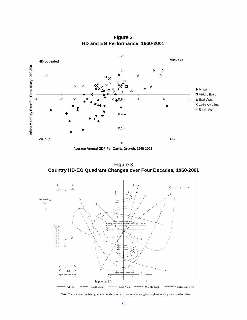
Figure 2HD and EG Performance, 1960-2001

0

0.2

0.4

0.6

0.8

1

1.2

-4 -2 0 2 4 6 8

Average Annual GDP Per Capita Growth, 1960-2001

Infa

nt

Mo

rtal

ity

Sh

ort

fall

Red

uct

ion

, 196

0-20

01

Africa

Middle East

East Asia

Latin America

South Asia

HD-Lopsided

EG-

Virtuous

Vicious

Figure 3 Country HD-EG Quadrant Changes over Four Decades, 1960-2001

Africa South Asia East Asia Middle East Latin America

Improving HD

Improving EG

3

2

2

9

2

2

3

2

9

2

2

2

12

2

Note: The numbers on this figure refer to the number of countries (in a given region) making the transition shown.

ETH

TGO

LSO

GNBKEN GAB

MLI

SLE

MRT

SOM

NGA TCDNER

ZAF

NAMSENBDI

UGALBR

GMBSDN

ZMB

MWI

ZWECOG

CMR

MUS

BENRWA

GHACIV

ZAR

BFA

MDG

CAF

TURPHL

HKG

BGD

NPL

KOR

AFG

CHN

PAKINDPNG

LKA

SGP

MYS

KHM

THA

IDN

NIC

PRYDOMCRI

VENPER

CHL

HND

BOLCOL SLVARG

ECUJAM

BRAPAN

URYMEX

TTO GTMHTI

SYR

OMNMAR

DZA

LBY

JOR

EGYARE

SAUIRQ

IRN

KWT TUN

-.5

0.5

-.5

0.5

-.5

0.5

-.5

0.5

0 200 0 200

0 200 0 200

Africa Asia

Latin America Middle East

Est

imat

ed G

row

th T

raje

ctor

y C

oeffi

cien

t

Early Infant Mortality Rate, 1960-1980

Explaining Growth Trajectories with Early IMR

Figure 4

ZAF

NER

GMB BEN

SOM

COG

NGA

MUS

GABGNB MWI

MLI

BDISDN

TCDZWECMR

UGA

GHA

NAM

ZAR

CAF

SLE

LSO

TGO

ZMB

SEN KENRWACIV

BFA

ETH

MDGLBR

MRT

KHM

SGP

THA

AFGNPL

BGD

HKG

PHLTURPAK

LKA

KOR

IND

MYS

IDN

CHN

PNG

ECU JAM

HNDPER

PRYMEX

CRICHLDOM

GTMHTI

URY

VEN

BOLSLV ARGCOL

BRA

TTOPAN

NIC

IRNLBY

TUNSAU

EGY

SYR

MARIRQ

KWT

ARE

DZAOMN

-.5

0.5

-.5

0.5

-.5

0.5

-.5

0.5

40 60 80 40 60 80

40 60 80 40 60 80

Africa Asia

Latin America Middle East

Est

imat

ed G

row

th T

raje

ctor

y C

oeffi

cien

t

Early Life Expectancy, 1960-1980

Explaining Growth Trajectories with Early LE

Figure 5

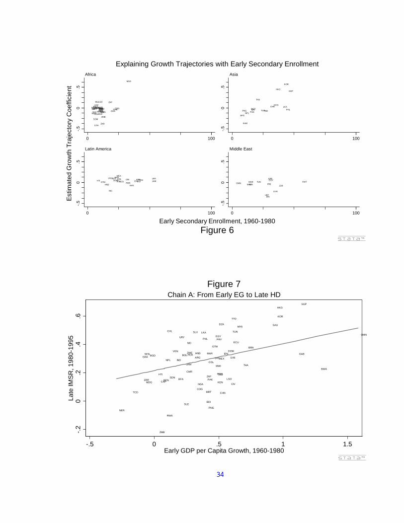
SOM

BDICMR

LBRTCD

KENTGO

ZAR

NER

COGGHA

UGA

GABGNBSEN

ETH

RWASDNCIV

LSO

BFA

ZAF

ZWEMDGNGAMRTBENMWI

SLE

MUS

ZMB

GMBCAF

MLI

KOR

MYS

PAKNPLPNG

CHN

AFG

IDN PHL

KHM

INDTUR

THA

HKGSGP

LKABGD

ARG

PER

URYJAMBOLHTI

SLV COL CRI

VENHND

PANPRY

MEX

CHLECU TTO

BRADOM

GTM

NIC

DZAMAR TUN

EGY

IRQ

IRN

OMN

SYR

LBY

KWTSAU

JOR

ARE

-.5

0.5

-.5

0.5

-.5

0.5

-.5

0.5

0 100 0 100

0 100 0 100

Africa Asia

Latin America Middle East

Est

imat

ed G

row

th T

raje

ctor

y C

oeffi

cien

t

Early Secondary Enrollment, 1960-1980

Explaining Growth Trajectories with Early Secondary Enrollment

Figure 6

NER

TCD

GHA

ZAR

SEN

MDG

BGD

HTI

ZMB

CAFBEN

NPL

RWA

CHL

SDN

VEN

IND

BFA

URY

BOL

SLE

JAM

CMR

ZWE

NIC

PER

SLV

ARG

HND

COG

NGA

LKA

PHL

MRT

BDI

ZAF

MAR

PAK

COL

PNG

GTM

CRI

EGY

MWI

PRY

PANTGO

KEN

MEX

DZA

CHN

IDN

LSO

DOM

SYR

CIV

TTO

TUN

ECU

MYS

THA

BRA

SAU

HKG

KOR

GAB

SGP

BWA

OMN

-.2

0.2

.4.6

Late

IMS

R, 1

980-

1995

-.5 0 .5 1 1.5Early GDP per Capita Growth, 1960-1980

Chain A: From Early EG to Late HDFigure 7

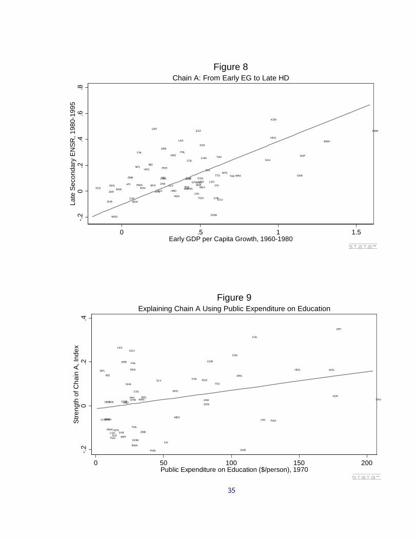
TCD

GHA

ZAR

SEN

MDG

BGD

HTI

ZMB

CAFBEN

NPL

RWA

CHL

SDN

VEN

IND

BFA

URY

BOLSLE

JAM

CMR

ZWE

NIC

PER

SLV

ARG

HND

NGA

LKA

PHL

MRTBDI

MARPAK

COL

PNG

GTM

CRI

EGY

MWIPRY

PAN

TGO

KEN

MEX

DZA

CHN

IDN

LSO

DOM

SYR

CIV

TTO

TUN

ECU

MYSTHA BRA

SAU

HKG

KOR

GAB

SGP

BWA

OMN

-.2

0.2

.4.6

.8La

te S

econ

dary

EN

SR

, 198

0-19

95

0 .5 1 1.5Early GDP per Capita Growth, 1960-1980

Chain A: From Early EG to Late HDFigure 8

NPL

CHN

NER

PAK

IND

MWI

RWA

IDN

LSO

TGOSLE

KEN

LKA

SYR

MRT

ZWE

CMRHND

GHA

EGY

PRY

SEN

GTM

PHL

THA

BWA

DOM

COL

MAR

ZMB

BOL

PNG

SLV

CIV

MYS

MEX

TUN PER

JAM

SDN

KOR

TTO

DZA

ARG

GAB

CHL

CRI PAN

HKG VEN

SGP

URY

SAU

-.2

0.2

.4S

tren

gth

of C

hain

A, I

ndex

0 50 100 150 200Public Expenditure on Education ($/person), 1970

Explaining Chain A Using Public Expenditure on EducationFigure 9

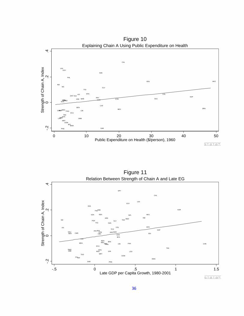
CHN

IND

LSO

MWI

ZMB

LKA

SDN

PNG

MDG

NIC

NER

KEN

MRT

EGY

IDN

THA

HND

DOM

PAN

PHL

BDI

ZAR

BWA

ECU

TCD

JAM

BEN

HTI

OMN

CRI

MAR

TTO

MYS

PRYCMR

DZA

CAF

GAB

SLV

GTM

MEX

CHL

VEN

SAU

COL

SGP

BRA

HKG

-.2

0.2

.4S

tren

gth

of C

hain

A, I

ndex

0 10 20 30 40 50Public Expenditure on Health ($/person), 1960

Explaining Chain A Using Public Expenditure on HealthFigure 10

NIC

HTI

RWA

SAU

ZMB

NER CMR

CIVBDI

MDG

CAF

TGO

GAB

DZA

VEN

PER

PRY

PHL

TTO

ECU

NGA

BOL

ZWE

HND

KEN

GTM

SEN

MRT

MEXBEN

MWI

ARG

PAN

SYR

BRA

GHA

PNG

JAM

TCD

MAR

SLV

COL

SDN

BFA

URY

CRI

DOM

TUNBGD

EGY

PAK

NPL

LSO

LKA

IND

HKG

MYS

IDN

BWA

CHL

SGP

THA

KOR

CHN

-.2

0.2

.4S

tren

gth

of C

hain

A, I

ndex

-.5 0 .5 1 1.5Late GDP per Capita Growth, 1980-2001

Relation Between Strength of Chain A and Late EGFigure 11

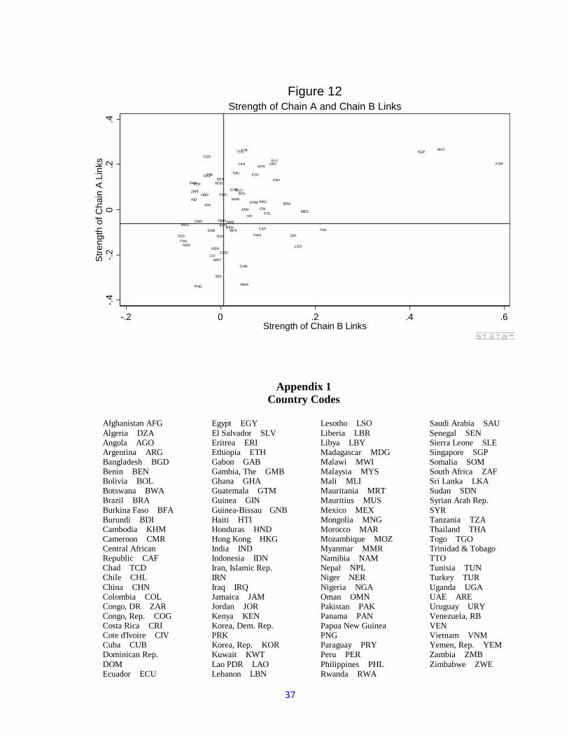
DZA

ARG

BGD

BEN

BOL

BRA

BFA

BDI

CMR

CAF

TCD

CHL

CHN

COL

COG

CRI

CIV

DOM

ECU

EGY

SLV

GAB

GHA

GTM

HTI

HND

HKG

IND

IDNJAM

KEN

KOR

LSO

MDGMWI

MYS

MRT

MEX

MAR

NGA

OMN

PAK

PAN

PNG

PRY

PER

PHL

RWA

SAUSEN

SGP

ZAF

LKA

SDNTHA

TGO

TTO

TUN

URY

VEN

ZWE

-.4

-.2

0.2

.4S

tren

gth

of C

hain

A L

inks

-.2 0 .2 .4 .6Strength of Chain B Links

Strength of Chain A and Chain B LinksFigure 12

Appendix 1 Country Codes

Afghanistan AFG Algeria DZA Angola AGO Argentina ARG Bangladesh BGD Benin BEN Bolivia BOL Botswana BWA Brazil BRA Burkina Faso BFA Burundi BDI Cambodia KHM Cameroon CMR Central African Republic CAF Chad TCD Chile CHL China CHN Colombia COL Congo, DR ZAR Congo, Rep. COG Costa Rica CRI Cote d'Ivoire CIV Cuba CUB Dominican Rep. DOM Ecuador ECU

Egypt EGY El Salvador SLV Eritrea ERI Ethiopia ETH Gabon GAB Gambia, The GMB Ghana GHA Guatemala GTM Guinea GIN Guinea-Bissau GNB Haiti HTI Honduras HND Hong Kong HKG India IND Indonesia IDN Iran, Islamic Rep. IRN Iraq IRQ Jamaica JAM Jordan JOR Kenya KEN Korea, Dem. Rep. PRK Korea, Rep. KOR Kuwait KWT Lao PDR LAO Lebanon LBN

Lesotho LSO Liberia LBR Libya LBY Madagascar MDG Malawi MWI Malaysia MYS Mali MLI Mauritania MRT Mauritius MUS Mexico MEX Mongolia MNG Morocco MAR Mozambique MOZ Myanmar MMR Namibia NAM Nepal NPL Niger NER Nigeria NGA Oman OMN Pakistan PAK Panama PAN Papua New Guinea PNG Paraguay PRY Peru PER Philippines PHL Rwanda RWA

Saudi Arabia SAU Senegal SEN Sierra Leone SLE Singapore SGP Somalia SOM South Africa ZAF Sri Lanka LKA Sudan SDN Syrian Arab Rep. SYR Tanzania TZA Thailand THA Togo TGO Trinidad & Tobago TTO Tunisia TUN Turkey TUR Uganda UGA UAE ARE Uruguay URY Venezuela, RB VEN Vietnam VNM Yemen, Rep. YEM Zambia ZMB Zimbabwe ZWE

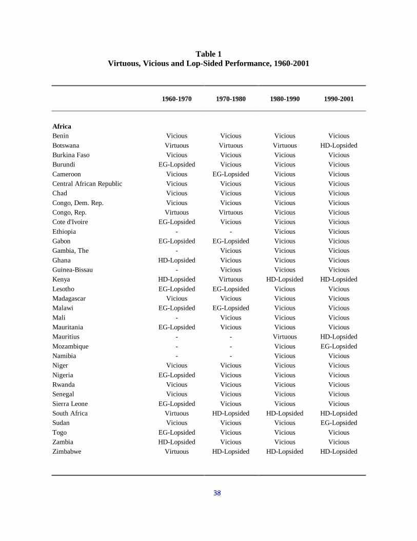
Table 1 Virtuous, Vicious and Lop-Sided Performance, 1960-2001

1960-1970

1970-1980

1980-1990

1990-2001

Africa Benin Vicious Vicious Vicious Vicious

Botswana Virtuous Virtuous Virtuous HD-Lopsided Burkina Faso Vicious Vicious Vicious Vicious Burundi EG-Lopsided Vicious Vicious Vicious

Cameroon Vicious EG-Lopsided Vicious Vicious Central African Republic Vicious Vicious Vicious Vicious Chad Vicious Vicious Vicious Vicious

Congo, Dem. Rep. Vicious Vicious Vicious Vicious Congo, Rep. Virtuous Virtuous Vicious Vicious Cote d'Ivoire EG-Lopsided Vicious Vicious Vicious

Ethiopia - - Vicious Vicious Gabon EG-Lopsided EG-Lopsided Vicious Vicious Gambia, The - Vicious Vicious Vicious

Ghana HD-Lopsided Vicious Vicious Vicious Guinea-Bissau - Vicious Vicious Vicious Kenya HD-Lopsided Virtuous HD-Lopsided HD-Lopsided

Lesotho EG-Lopsided EG-Lopsided Vicious Vicious Madagascar Vicious Vicious Vicious Vicious Malawi EG-Lopsided EG-Lopsided Vicious Vicious

Mali - Vicious Vicious Vicious Mauritania EG-Lopsided Vicious Vicious Vicious Mauritius - - Virtuous HD-Lopsided

Mozambique - - Vicious EG-Lopsided Namibia - - Vicious Vicious Niger Vicious Vicious Vicious Vicious

Nigeria EG-Lopsided Vicious Vicious Vicious Rwanda Vicious Vicious Vicious Vicious Senegal Vicious Vicious Vicious Vicious

Sierra Leone EG-Lopsided Vicious Vicious Vicious South Africa Virtuous HD-Lopsided HD-Lopsided HD-Lopsided Sudan Vicious Vicious Vicious EG-Lopsided

Togo EG-Lopsided Vicious Vicious Vicious Zambia HD-Lopsided Vicious Vicious Vicious Zimbabwe Virtuous HD-Lopsided HD-Lopsided HD-Lopsided

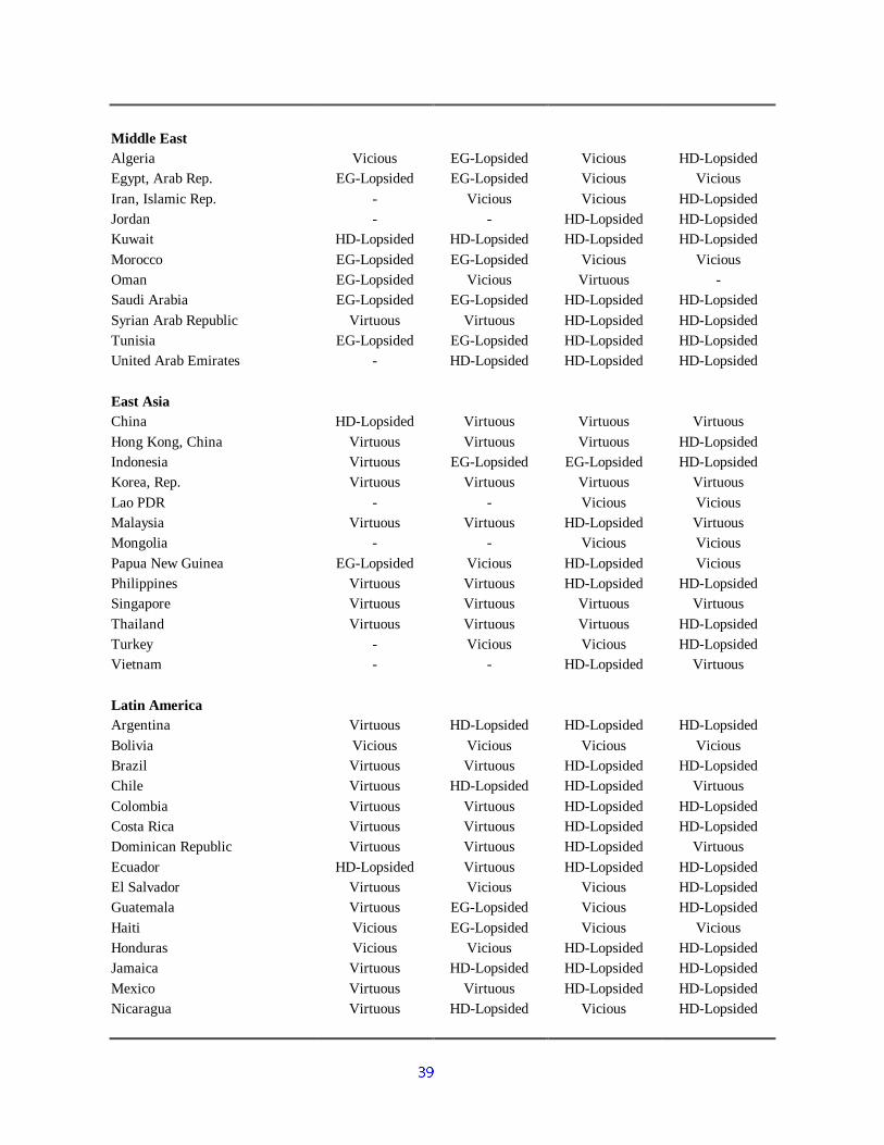
Middle East Algeria Vicious EG-Lopsided Vicious HD-Lopsided Egypt, Arab Rep. EG-Lopsided EG-Lopsided Vicious Vicious

Iran, Islamic Rep. - Vicious Vicious HD-Lopsided Jordan - - HD-Lopsided HD-Lopsided Kuwait HD-Lopsided HD-Lopsided HD-Lopsided HD-Lopsided

Morocco EG-Lopsided EG-Lopsided Vicious Vicious Oman EG-Lopsided Vicious Virtuous - Saudi Arabia EG-Lopsided EG-Lopsided HD-Lopsided HD-Lopsided

Syrian Arab Republic Virtuous Virtuous HD-Lopsided HD-Lopsided Tunisia EG-Lopsided EG-Lopsided HD-Lopsided HD-Lopsided United Arab Emirates - HD-Lopsided HD-Lopsided HD-Lopsided

East Asia China HD-Lopsided Virtuous Virtuous Virtuous

Hong Kong, China Virtuous Virtuous Virtuous HD-Lopsided Indonesia Virtuous EG-Lopsided EG-Lopsided HD-Lopsided Korea, Rep. Virtuous Virtuous Virtuous Virtuous

Lao PDR - - Vicious Vicious Malaysia Virtuous Virtuous HD-Lopsided Virtuous Mongolia - - Vicious Vicious

Papua New Guinea EG-Lopsided Vicious HD-Lopsided Vicious Philippines Virtuous Virtuous HD-Lopsided HD-Lopsided Singapore Virtuous Virtuous Virtuous Virtuous

Thailand Virtuous Virtuous Virtuous HD-Lopsided Turkey - Vicious Vicious HD-Lopsided Vietnam - - HD-Lopsided Virtuous

Latin America Argentina Virtuous HD-Lopsided HD-Lopsided HD-Lopsided

Bolivia Vicious Vicious Vicious Vicious Brazil Virtuous Virtuous HD-Lopsided HD-Lopsided Chile Virtuous HD-Lopsided HD-Lopsided Virtuous

Colombia Virtuous Virtuous HD-Lopsided HD-Lopsided Costa Rica Virtuous Virtuous HD-Lopsided HD-Lopsided Dominican Republic Virtuous Virtuous HD-Lopsided Virtuous

Ecuador HD-Lopsided Virtuous HD-Lopsided HD-Lopsided El Salvador Virtuous Vicious Vicious HD-Lopsided Guatemala Virtuous EG-Lopsided Vicious HD-Lopsided

Haiti Vicious EG-Lopsided Vicious Vicious Honduras Vicious Vicious HD-Lopsided HD-Lopsided Jamaica Virtuous HD-Lopsided HD-Lopsided HD-Lopsided

Mexico Virtuous Virtuous HD-Lopsided HD-Lopsided Nicaragua Virtuous HD-Lopsided Vicious HD-Lopsided

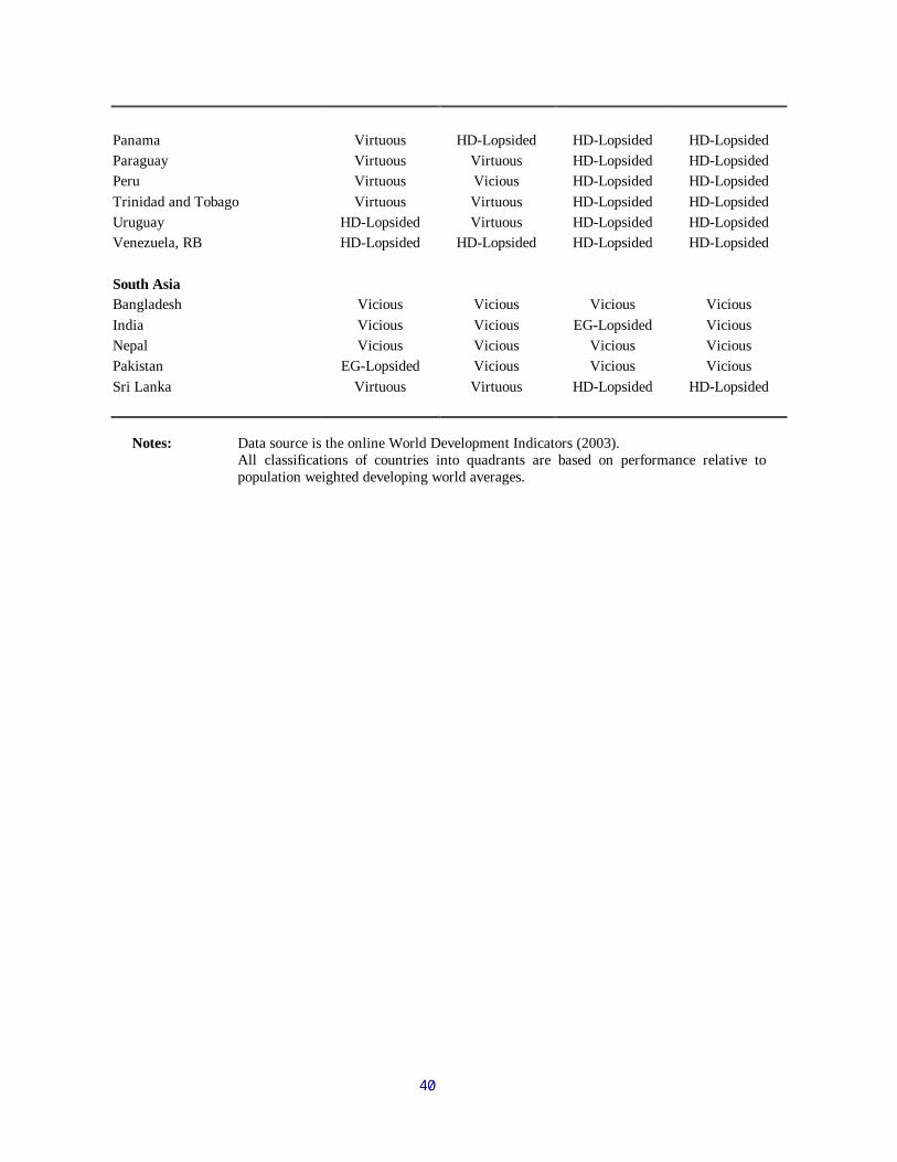
Panama Virtuous HD-Lopsided HD-Lopsided HD-Lopsided Paraguay Virtuous Virtuous HD-Lopsided HD-Lopsided Peru Virtuous Vicious HD-Lopsided HD-Lopsided

Trinidad and Tobago Virtuous Virtuous HD-Lopsided HD-Lopsided Uruguay HD-Lopsided Virtuous HD-Lopsided HD-Lopsided Venezuela, RB HD-Lopsided HD-Lopsided HD-Lopsided HD-Lopsided

South Asia Bangladesh Vicious Vicious Vicious Vicious

India Vicious Vicious EG-Lopsided Vicious Nepal Vicious Vicious Vicious Vicious Pakistan EG-Lopsided Vicious Vicious Vicious

Sri Lanka Virtuous Virtuous HD-Lopsided HD-Lopsided

Notes: Data source is the online World Development Indicators (2003).

All classifications of countries into quadrants are based on performance relative to population weighted developing world averages.

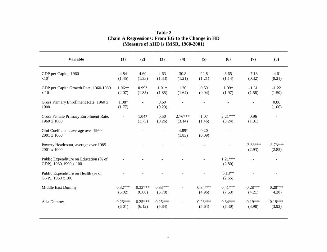
Table 2 Chain A Regressions: From EG to the Change in HD

(Measure of ∆HD is IMSR, 1960-2001)

Variable

(1)

(2)

(3)

(4)

(5)

(6)

(7)

(8)

GDP per Capita, 1960 x106

4.84 (1.45)

4.60 (1.33)

4.63 (1.33)

30.8 (1.21)

22.8 (1.21)

3.65 (1.14)

-7.13 (0.32)

-4.61 (0.21)

GDP per Capita Growth Rate, 1960-1980 x 10

1.06** (2.07)

0.99* (1.85)

1.01* (1.85)

1.30 (1.64)

0.59 (0.94)

1.09* (1.97)

-1.31 (1.58)

-1.22 (1.50)

Gross Primary Enrollment Rate, 1960 x 1000

1.08* (1.77)

- 0.60 (0.29)

- - - - 0.86 (1.06)

Gross Female Primary Enrollment Rate, 1960 x 1000

- 1.04* (1.73)

0.50 (0.26)

2.76*** (3.14)

1.07 (1.46)

2.21*** (3.24)

0.96 (1.31)

-

Gini Coefficient, average over 1960-2001 x 1000

- - - -4.89* (1.83)

0.20 (0.09)

- - -

Poverty Headcount, average over 1985-2001 x 1000

- - - - - - -3.83*** (2.93)

-3.73*** (2.85)

Public Expenditure on Education (% of GDP), 1980-1990 x 100

- - - - - 1.21*** (2.80)

- -

Public Expenditure on Health (% of GNP), 1960 x 100

- - - - - 6.13** (2.65)

- -

Middle East Dummy 0.32***

(6.02) 0.33*** (6.08)

0.33*** (5.70)

- 0.34*** (4.96)

0.41*** (7.53)

0.28*** (4.21)

0.28*** (4.20)

Asia Dummy 0.25***

(6.01) 0.25*** (6.12)

0.25*** (5.84)

- 0.28*** (5.64)

0.34*** (7.30)

0.19*** (3.98)

0.19*** (3.93)

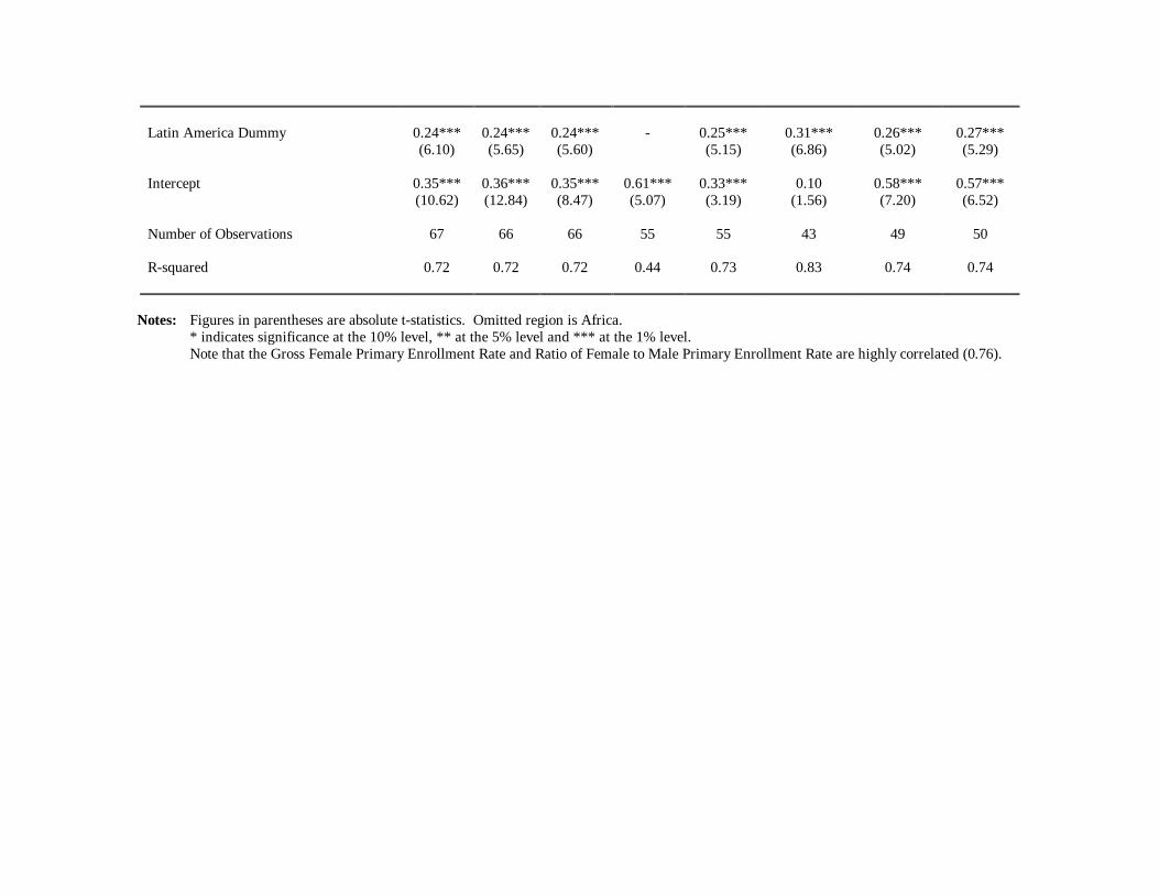
Latin America Dummy 0.24***

(6.10) 0.24*** (5.65)

0.24*** (5.60)

- 0.25*** (5.15)

0.31*** (6.86)

0.26*** (5.02)

0.27*** (5.29)

Intercept 0.35***

(10.62) 0.36*** (12.84)

0.35*** (8.47)

0.61*** (5.07)

0.33*** (3.19)

0.10 (1.56)

0.58*** (7.20)

0.57*** (6.52)

Number of Observations 67 66 66 55 55 43 49 50 R-squared 0.72 0.72 0.72 0.44 0.73 0.83 0.74 0.74

Notes: Figures in parentheses are absolute t-statistics. Omitted region is Africa.

* indicates significance at the 10% level, ** at the 5% level and *** at the 1% level. Note that the Gross Female Primary Enrollment Rate and Ratio of Female to Male Primary Enrollment Rate are highly correlated (0.76).

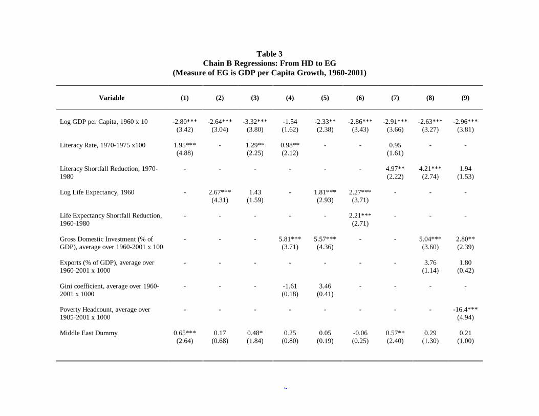
Table 3 Chain B Regressions: From HD to EG

(Measure of EG is GDP per Capita Growth, 1960-2001)

Variable

(1)

(2)

(3)

(4)

(5)

(6)

(7)

(8)

(9)

Log GDP per Capita, 1960 x 10 -2.80***

(3.42) -2.64***

(3.04) -3.32***

(3.80) -1.54 (1.62)

-2.33** (2.38)

-2.86*** (3.43)

-2.91*** (3.66)

-2.63*** (3.27)

-2.96*** (3.81)

Literacy Rate, 1970-1975 x100 1.95***

(4.88) - 1.29**

(2.25) 0.98** (2.12)

- - 0.95 (1.61)

- -

Literacy Shortfall Reduction, 1970-1980

- - - - - - 4.97** (2.22)

4.21*** (2.74)

1.94 (1.53)

Log Life Expectancy, 1960 - 2.67***

(4.31) 1.43

(1.59) - 1.81***

(2.93) 2.27*** (3.71)

- - -

Life Expectancy Shortfall Reduction, 1960-1980

- - - - - 2.21*** (2.71)

- - -

Gross Domestic Investment (% of GDP), average over 1960-2001 x 100

- - - 5.81*** (3.71)

5.57*** (4.36)

- - 5.04*** (3.60)

2.80** (2.39)

Exports (% of GDP), average over 1960-2001 x 1000

- - - - - - - 3.76 (1.14)

1.80 (0.42)

Gini coefficient, average over 1960-2001 x 1000

- - - -1.61 (0.18)

3.46 (0.41)

- - - -

Poverty Headcount, average over 1985-2001 x 1000

- - - - - - - - -16.4*** (4.94)

Middle East Dummy 0.65***

(2.64) 0.17

(0.68) 0.48* (1.84)

0.25 (0.80)

0.05 (0.19)

-0.06 (0.25)

0.57** (2.40)

0.29 (1.30)

0.21 (1.00)

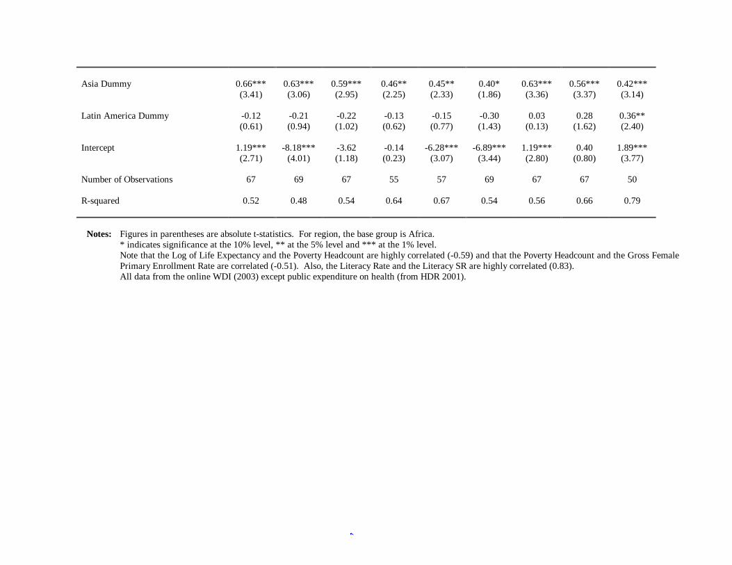
Asia Dummy 0.66***

(3.41) 0.63*** (3.06)

0.59*** (2.95)

0.46** (2.25)

0.45** (2.33)

0.40* (1.86)

0.63*** (3.36)

0.56*** (3.37)

0.42*** (3.14)

Latin America Dummy -0.12

(0.61) -0.21 (0.94)

-0.22 (1.02)

-0.13 (0.62)

-0.15 (0.77)

-0.30 (1.43)

0.03 (0.13)

0.28 (1.62)

0.36** (2.40)

Intercept 1.19***

(2.71) -8.18***

(4.01) -3.62 (1.18)

-0.14 (0.23)

-6.28*** (3.07)

-6.89*** (3.44)

1.19*** (2.80)

0.40 (0.80)

1.89*** (3.77)

Number of Observations 67 69 67 55 57 69 67 67 50 R-squared 0.52 0.48 0.54 0.64 0.67 0.54 0.56 0.66 0.79

Notes: Figures in parentheses are absolute t-statistics. For region, the base group is Africa.

* indicates significance at the 10% level, ** at the 5% level and *** at the 1% level. Note that the Log of Life Expectancy and the Poverty Headcount are highly correlated (-0.59) and that the Poverty Headcount and the Gross Female Primary Enrollment Rate are correlated (-0.51). Also, the Literacy Rate and the Literacy SR are highly correlated (0.83). All data from the online WDI (2003) except public expenditure on health (from HDR 2001).

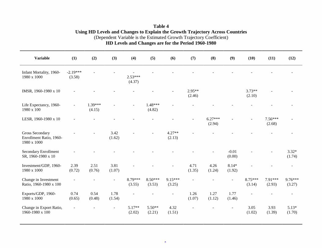
Table 4 Using HD Levels and Changes to Explain the Growth Trajectory Across Countries

(Dependent Variable is the Estimated Growth Trajectory Coefficient) HD Levels and Changes are for the Period 1960-1980

Variable

(1)

(2)

(3)

(4)

(5)

(6)

(7)

(8)

(9)

(10)

(11)

(12)

Infant Mortality, 1960-1980 x 1000

-2.19*** (3.58)

- - -2.53*** (4.37)

- - - - - - - -

IMSR, 1960-1980 x 10 - - - - - - 2.95**

(2.46) 3.73**

(2.10) - -

Life Expectancy, 1960-1980 x 100

- 1.39*** (4.15)

- - 1.48*** (4.82)

- - - - - - -

LESR, 1960-1980 x 10 - - - - - - - 6.27***

(2.94) - - 7.56***

(2.68) -

Gross Secondary Enrollment Ratio, 1960-1980 x 1000

- - 3.42 (1.62)

- - 4.27** (2.13)

- - - - - -

Secondary Enrollment SR, 1960-1980 x 10

- - - - - - - - -0.01 (0.00)

- - 3.32* (1.74)

Investment/GDP, 1960-1980 x 1000

2.39 (0.72)

2.51 (0.76)

3.81 (1.07)

- - - 4.71 (1.35)

4.26 (1.24)

8.14* (1.92)

- - -

Change in Investment Ratio, 1960-1980 x 100

- - - 8.79*** (3.55)

8.50*** (3.53)

9.15*** (3.25)

- - - 8.75*** (3.14)

7.91*** (2.93)

9.76*** (3.27)

Exports/GDP, 1960-1980 x 1000

0.74 (0.65)

0.54 (0.48)

1.78 (1.54)

- - - 1.26 (1.07)

1.27 (1.12)

1.77 (1.46)

- - -

Change in Export Ratio, 1960-1980 x 100

- - - 5.17** (2.02)

5.50** (2.21)

4.32 (1.51)

- - - 3.05 (1.02)

3.93 (1.39)

5.13* (1.70)

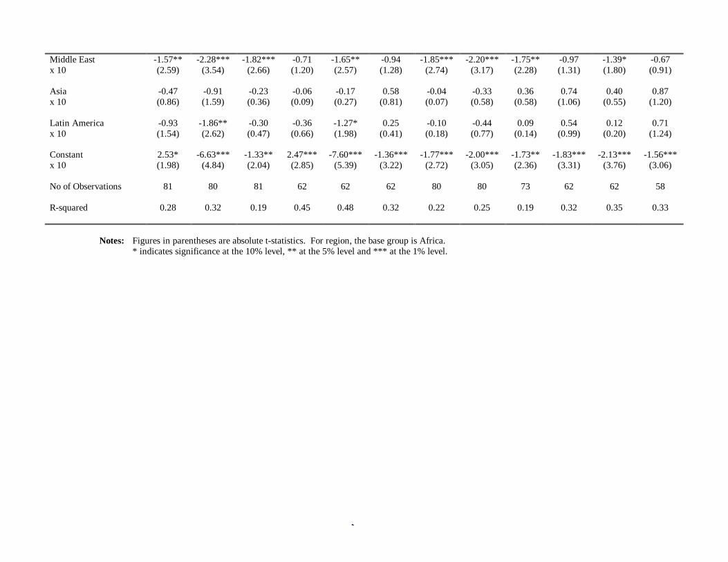
Middle East x 10

-1.57** (2.59)

-2.28*** (3.54)

-1.82*** (2.66)

-0.71 (1.20)

-1.65** (2.57)

-0.94 (1.28)

-1.85*** (2.74)

-2.20*** (3.17)

-1.75** (2.28)

-0.97 (1.31)

-1.39* (1.80)

-0.67 (0.91)

Asia x 10

-0.47 (0.86)

-0.91 (1.59)

-0.23 (0.36)

-0.06 (0.09)

-0.17 (0.27)

0.58 (0.81)

-0.04 (0.07)

-0.33 (0.58)

0.36 (0.58)

0.74 (1.06)

0.40 (0.55)

0.87 (1.20)

Latin America x 10

-0.93 (1.54)

-1.86** (2.62)

-0.30 (0.47)

-0.36 (0.66)

-1.27* (1.98)

0.25 (0.41)

-0.10 (0.18)

-0.44 (0.77)

0.09 (0.14)

0.54 (0.99)

0.12 (0.20)

0.71 (1.24)

Constant x 10

2.53* (1.98)

-6.63*** (4.84)

-1.33** (2.04)

2.47*** (2.85)

-7.60*** (5.39)

-1.36*** (3.22)

-1.77*** (2.72)

-2.00*** (3.05)

-1.73** (2.36)

-1.83*** (3.31)

-2.13*** (3.76)

-1.56*** (3.06)

No of Observations 81 80 81 62 62 62 80 80 73 62 62 58 R-squared 0.28 0.32 0.19 0.45 0.48 0.32 0.22 0.25 0.19 0.32 0.35 0.33

Notes: Figures in parentheses are absolute t-statistics. For region, the base group is Africa.

* indicates significance at the 10% level, ** at the 5% level and *** at the 1% level.

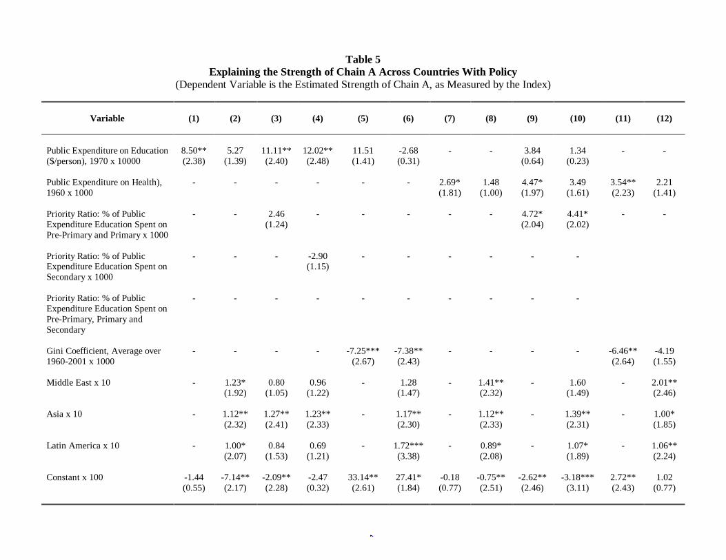
Table 5 Explaining the Strength of Chain A Across Countries With Policy

(Dependent Variable is the Estimated Strength of Chain A, as Measured by the Index)

Variable

(1)

(2)

(3)

(4)

(5)

(6)

(7)

(8)

(9)

(10)

(11)

(12)

Public Expenditure on Education ($/person), 1970 x 10000

8.50** (2.38)

5.27 (1.39)

11.11** (2.40)

12.02** (2.48)

11.51 (1.41)

-2.68 (0.31)

- - 3.84 (0.64)

1.34 (0.23)

- -

Public Expenditure on Health), 1960 x 1000

- - - - - - 2.69* (1.81)

1.48 (1.00)

4.47* (1.97)

3.49 (1.61)

3.54** (2.23)

2.21 (1.41)

Priority Ratio: % of Public Expenditure Education Spent on Pre-Primary and Primary x 1000

- - 2.46 (1.24)

- - - - - 4.72* (2.04)

4.41* (2.02)

- -

Priority Ratio: % of Public Expenditure Education Spent on Secondary x 1000

- - - -2.90 (1.15)

- - - - - -

Priority Ratio: % of Public Expenditure Education Spent on Pre-Primary, Primary and Secondary

- - - - - - - - - -

Gini Coefficient, Average over 1960-2001 x 1000

- - - - -7.25*** (2.67)

-7.38** (2.43)

- - - - -6.46** (2.64)

-4.19 (1.55)

Middle East x 10 - 1.23*

(1.92) 0.80

(1.05) 0.96

(1.22) - 1.28

(1.47) -

1.41** (2.32)

- 1.60 (1.49)

- 2.01** (2.46)

Asia x 10 - 1.12**

(2.32) 1.27** (2.41)

1.23** (2.33)

- 1.17** (2.30)

-

1.12** (2.33)

- 1.39** (2.31)

- 1.00* (1.85)

Latin America x 10 - 1.00*

(2.07) 0.84

(1.53) 0.69

(1.21) - 1.72***

(3.38) -

0.89* (2.08)

- 1.07* (1.89)

- 1.06** (2.24)

Constant x 100 -1.44

(0.55) -7.14** (2.17)

-2.09** (2.28)

-2.47 (0.32)

33.14** (2.61)

27.41* (1.84)

-0.18 (0.77)

-0.75** (2.51)

-2.62** (2.46)

-3.18*** (3.11)

2.72** (2.43)

1.02 (0.77)

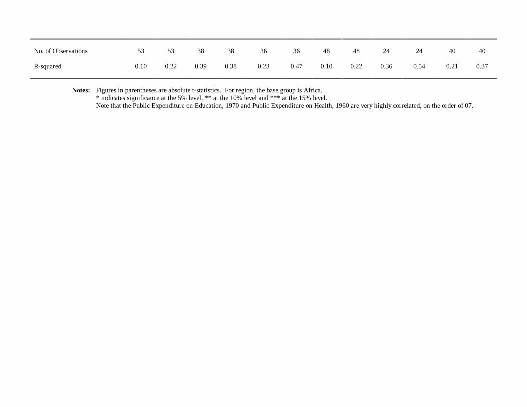
No. of Observations 53 53 38 38 36 36 48 48 24 24 40 40 R-squared 0.10 0.22 0.39 0.38 0.23 0.47 0.10 0.22 0.36 0.54 0.21 0.37

Notes: Figures in parentheses are absolute t-statistics. For region, the base group is Africa.

* indicates significance at the 5% level, ** at the 10% level and *** at the 15% level. Note that the Public Expenditure on Education, 1970 and Public Expenditure on Health, 1960 are very highly correlated, on the order of 07.