pattern recognition and machine learning - … · mixture models and em ... pattern recognition,...

9Mixture Models

and EM

If we define a joint distribution over observed and latent variables, the correspond-ing distribution of the observed variables alone is obtained by marginalization. Thisallows relatively complex marginal distributions over observed variables to be ex-pressed in terms of more tractable joint distributions over the expanded space ofobserved and latent variables. The introduction of latent variables thereby allowscomplicated distributions to be formed from simpler components. In this chapter,we shall see that mixture distributions, such as the Gaussian mixture discussed inSection 2.3.9, can be interpreted in terms of discrete latent variables. Continuouslatent variables will form the subject of Chapter 12.

As well as providing a framework for building more complex probability dis-tributions, mixture models can also be used to cluster data. We therefore begin ourdiscussion of mixture distributions by considering the problem of finding clustersin a set of data points, which we approach first using a nonprobabilistic techniquecalled the K-means algorithm (Lloyd, 1982). Then we introduce the latent variableSection 9.1

423

424 9. MIXTURE MODELS AND EM

view of mixture distributions in which the discrete latent variables can be interpretedas defining assignments of data points to specific components of the mixture. A gen-Section 9.2eral technique for finding maximum likelihood estimators in latent variable modelsis the expectation-maximization (EM) algorithm. We first of all use the Gaussianmixture distribution to motivate the EM algorithm in a fairly informal way, and thenwe give a more careful treatment based on the latent variable viewpoint. We shallSection 9.3see that the K-means algorithm corresponds to a particular nonprobabilistic limit ofEM applied to mixtures of Gaussians. Finally, we discuss EM in some generality.Section 9.4

Gaussian mixture models are widely used in data mining, pattern recognition,machine learning, and statistical analysis. In many applications, their parameters aredetermined by maximum likelihood, typically using the EM algorithm. However, aswe shall see there are some significant limitations to the maximum likelihood ap-proach, and in Chapter 10 we shall show that an elegant Bayesian treatment can begiven using the framework of variational inference. This requires little additionalcomputation compared with EM, and it resolves the principal difficulties of maxi-mum likelihood while also allowing the number of components in the mixture to beinferred automatically from the data.

9.1. K-means Clustering

We begin by considering the problem of identifying groups, or clusters, of data pointsin a multidimensional space. Suppose we have a data set {x1, . . . ,xN} consistingof N observations of a random D-dimensional Euclidean variable x. Our goal is topartition the data set into some number K of clusters, where we shall suppose forthe moment that the value of K is given. Intuitively, we might think of a cluster ascomprising a group of data points whose inter-point distances are small comparedwith the distances to points outside of the cluster. We can formalize this notion byfirst introducing a set of D-dimensional vectors µk, where k = 1, . . . , K, in whichµk is a prototype associated with the kth cluster. As we shall see shortly, we canthink of the µk as representing the centres of the clusters. Our goal is then to findan assignment of data points to clusters, as well as a set of vectors {µk}, such thatthe sum of the squares of the distances of each data point to its closest vector µk, isa minimum.

It is convenient at this point to define some notation to describe the assignmentof data points to clusters. For each data point xn, we introduce a corresponding setof binary indicator variables rnk ∈ {0, 1}, where k = 1, . . . , K describing which ofthe K clusters the data point xn is assigned to, so that if data point xn is assigned tocluster k then rnk = 1, and rnj = 0 for j �= k. This is known as the 1-of-K codingscheme. We can then define an objective function, sometimes called a distortionmeasure, given by

J =N�

n=1

K�

k=1

rnk�xn − µk�2 (9.1)

which represents the sum of the squares of the distances of each data point to its

9.1. K-means Clustering 425

assigned vector µk. Our goal is to find values for the {rnk} and the {µk} so as tominimize J . We can do this through an iterative procedure in which each iterationinvolves two successive steps corresponding to successive optimizations with respectto the rnk and the µk. First we choose some initial values for the µk. Then in the firstphase we minimize J with respect to the rnk, keeping the µk fixed. In the secondphase we minimize J with respect to the µk, keeping rnk fixed. This two-stageoptimization is then repeated until convergence. We shall see that these two stagesof updating rnk and updating µk correspond respectively to the E (expectation) andM (maximization) steps of the EM algorithm, and to emphasize this we shall use theSection 9.4terms E step and M step in the context of the K-means algorithm.

Consider first the determination of the rnk. Because J in (9.1) is a linear func-tion of rnk, this optimization can be performed easily to give a closed form solution.The terms involving different n are independent and so we can optimize for eachn separately by choosing rnk to be 1 for whichever value of k gives the minimumvalue of �xn − µk�2. In other words, we simply assign the nth data point to theclosest cluster centre. More formally, this can be expressed as

rnk =�

1 if k = arg minj �xn − µj�2

0 otherwise.(9.2)

Now consider the optimization of the µk with the rnk held fixed. The objectivefunction J is a quadratic function of µk, and it can be minimized by setting itsderivative with respect to µk to zero giving

2N�

n=1

rnk(xn − µk) = 0 (9.3)

which we can easily solve for µk to give

µk =�

n rnkxn�n rnk

. (9.4)

The denominator in this expression is equal to the number of points assigned tocluster k, and so this result has a simple interpretation, namely set µk equal to themean of all of the data points xn assigned to cluster k. For this reason, the procedureis known as the K-means algorithm.

The two phases of re-assigning data points to clusters and re-computing the clus-ter means are repeated in turn until there is no further change in the assignments (oruntil some maximum number of iterations is exceeded). Because each phase reducesthe value of the objective function J , convergence of the algorithm is assured. How-Exercise 9.1ever, it may converge to a local rather than global minimum of J . The convergenceproperties of the K-means algorithm were studied by MacQueen (1967).

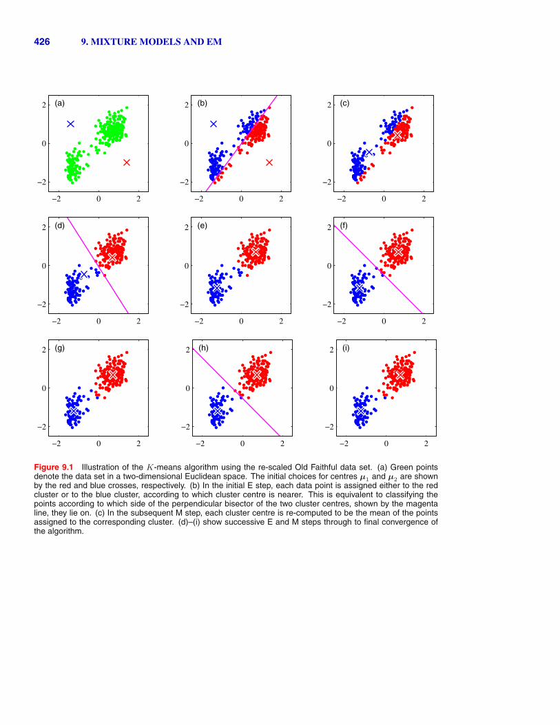
The K-means algorithm is illustrated using the Old Faithful data set in Fig-Appendix Aure 9.1. For the purposes of this example, we have made a linear re-scaling of thedata, known as standardizing, such that each of the variables has zero mean andunit standard deviation. For this example, we have chosen K = 2, and so in this


(a)

−2 0 2

−2

0

2 (b)

−2 0 2

−2

0

2 (c)

−2 0 2

−2

0

2

(d)

−2 0 2

−2

0

2 (e)

−2 0 2

−2

0

2 (f)

−2 0 2

−2

0

2

(g)

−2 0 2

−2

0

2 (h)

−2 0 2

−2

0

2 (i)

−2 0 2

−2

0

2

Figure 9.1 Illustration of the K-means algorithm using the re-scaled Old Faithful data set. (a) Green pointsdenote the data set in a two-dimensional Euclidean space. The initial choices for centres µ1 and µ2 are shownby the red and blue crosses, respectively. (b) In the initial E step, each data point is assigned either to the redcluster or to the blue cluster, according to which cluster centre is nearer. This is equivalent to classifying thepoints according to which side of the perpendicular bisector of the two cluster centres, shown by the magentaline, they lie on. (c) In the subsequent M step, each cluster centre is re-computed to be the mean of the pointsassigned to the corresponding cluster. (d)–(i) show successive E and M steps through to final convergence ofthe algorithm.


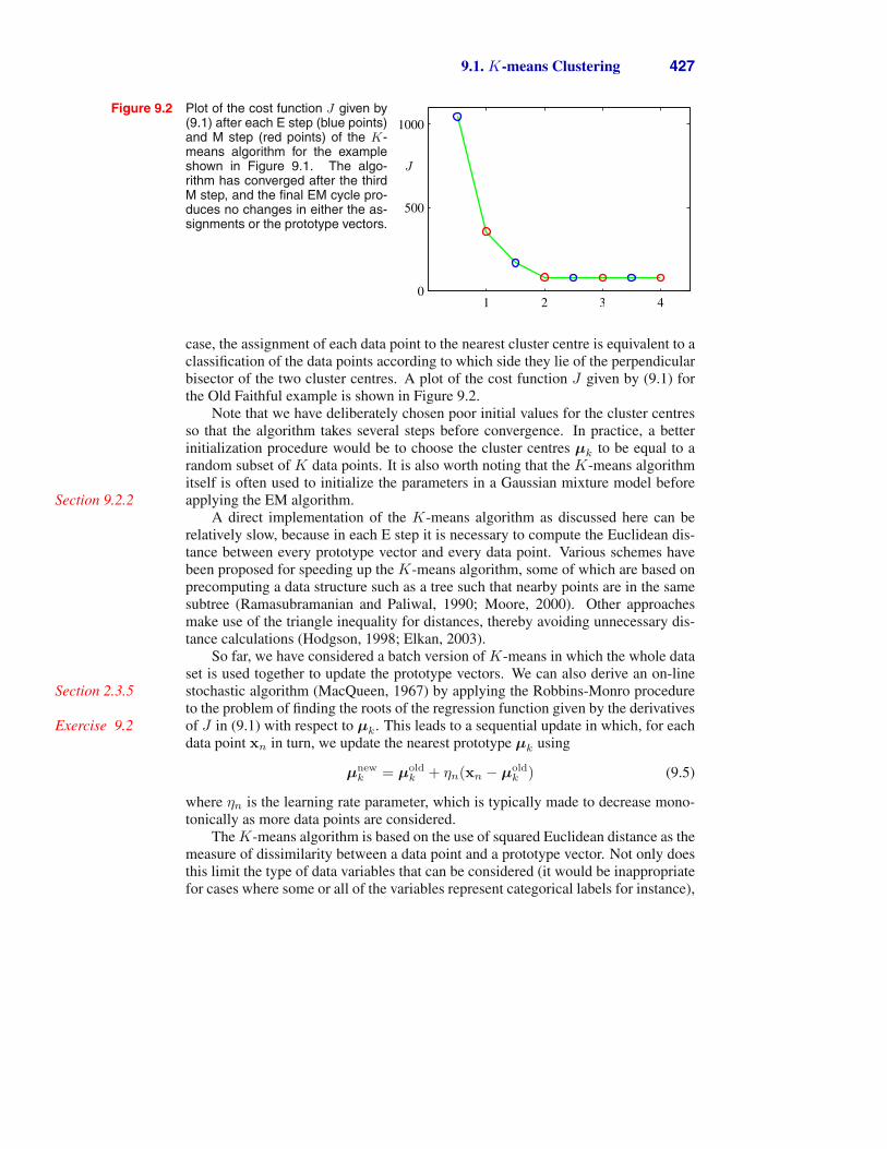
Figure 9.2 Plot of the cost function J given by(9.1) after each E step (blue points)and M step (red points) of the K-means algorithm for the exampleshown in Figure 9.1. The algo-rithm has converged after the thirdM step, and the final EM cycle pro-duces no changes in either the as-signments or the prototype vectors.

J

1 2 3 40

500

1000

case, the assignment of each data point to the nearest cluster centre is equivalent to aclassification of the data points according to which side they lie of the perpendicularbisector of the two cluster centres. A plot of the cost function J given by (9.1) forthe Old Faithful example is shown in Figure 9.2.

Note that we have deliberately chosen poor initial values for the cluster centresso that the algorithm takes several steps before convergence. In practice, a betterinitialization procedure would be to choose the cluster centres µk to be equal to arandom subset of K data points. It is also worth noting that the K-means algorithmitself is often used to initialize the parameters in a Gaussian mixture model beforeapplying the EM algorithm.Section 9.2.2

A direct implementation of the K-means algorithm as discussed here can berelatively slow, because in each E step it is necessary to compute the Euclidean dis-tance between every prototype vector and every data point. Various schemes havebeen proposed for speeding up the K-means algorithm, some of which are based onprecomputing a data structure such as a tree such that nearby points are in the samesubtree (Ramasubramanian and Paliwal, 1990; Moore, 2000). Other approachesmake use of the triangle inequality for distances, thereby avoiding unnecessary dis-tance calculations (Hodgson, 1998; Elkan, 2003).

So far, we have considered a batch version of K-means in which the whole dataset is used together to update the prototype vectors. We can also derive an on-linestochastic algorithm (MacQueen, 1967) by applying the Robbins-Monro procedureSection 2.3.5to the problem of finding the roots of the regression function given by the derivativesof J in (9.1) with respect to µk. This leads to a sequential update in which, for eachExercise 9.2data point xn in turn, we update the nearest prototype µk using

µnewk = µold

k + ηn(xn − µoldk ) (9.5)

where ηn is the learning rate parameter, which is typically made to decrease mono-tonically as more data points are considered.

The K-means algorithm is based on the use of squared Euclidean distance as themeasure of dissimilarity between a data point and a prototype vector. Not only doesthis limit the type of data variables that can be considered (it would be inappropriatefor cases where some or all of the variables represent categorical labels for instance),


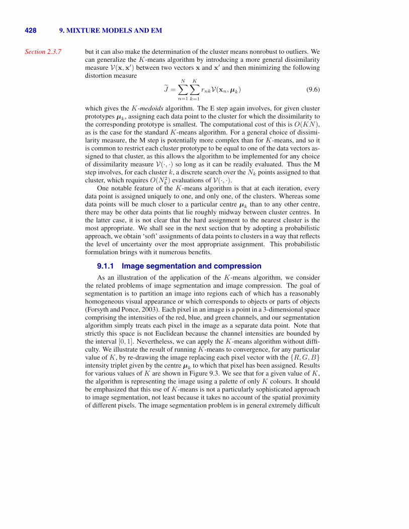
but it can also make the determination of the cluster means nonrobust to outliers. WeSection 2.3.7can generalize the K-means algorithm by introducing a more general dissimilaritymeasure V(x,x�) between two vectors x and x� and then minimizing the followingdistortion measure

�J =N�

n=1

K�

k=1

rnkV(xn, µk) (9.6)

which gives the K-medoids algorithm. The E step again involves, for given clusterprototypes µk, assigning each data point to the cluster for which the dissimilarity tothe corresponding prototype is smallest. The computational cost of this is O(KN),as is the case for the standard K-means algorithm. For a general choice of dissimi-larity measure, the M step is potentially more complex than for K-means, and so itis common to restrict each cluster prototype to be equal to one of the data vectors as-signed to that cluster, as this allows the algorithm to be implemented for any choiceof dissimilarity measure V(·, ·) so long as it can be readily evaluated. Thus the Mstep involves, for each cluster k, a discrete search over the Nk points assigned to thatcluster, which requires O(N2

k) evaluations of V(·, ·).One notable feature of the K-means algorithm is that at each iteration, every

data point is assigned uniquely to one, and only one, of the clusters. Whereas somedata points will be much closer to a particular centre µk than to any other centre,there may be other data points that lie roughly midway between cluster centres. Inthe latter case, it is not clear that the hard assignment to the nearest cluster is themost appropriate. We shall see in the next section that by adopting a probabilisticapproach, we obtain ‘soft’ assignments of data points to clusters in a way that reflectsthe level of uncertainty over the most appropriate assignment. This probabilisticformulation brings with it numerous benefits.

9.1.1 Image segmentation and compressionAs an illustration of the application of the K-means algorithm, we consider

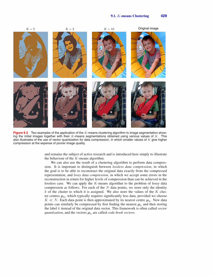
the related problems of image segmentation and image compression. The goal ofsegmentation is to partition an image into regions each of which has a reasonablyhomogeneous visual appearance or which corresponds to objects or parts of objects(Forsyth and Ponce, 2003). Each pixel in an image is a point in a 3-dimensional spacecomprising the intensities of the red, blue, and green channels, and our segmentationalgorithm simply treats each pixel in the image as a separate data point. Note thatstrictly this space is not Euclidean because the channel intensities are bounded bythe interval [0, 1]. Nevertheless, we can apply the K-means algorithm without diffi-culty. We illustrate the result of running K-means to convergence, for any particularvalue of K, by re-drawing the image replacing each pixel vector with the {R, G, B}intensity triplet given by the centre µk to which that pixel has been assigned. Resultsfor various values of K are shown in Figure 9.3. We see that for a given value of K,the algorithm is representing the image using a palette of only K colours. It shouldbe emphasized that this use of K-means is not a particularly sophisticated approachto image segmentation, not least because it takes no account of the spatial proximityof different pixels. The image segmentation problem is in general extremely difficult


K = 2 K = 3 K = 10 Original image

Figure 9.3 Two examples of the application of the K-means clustering algorithm to image segmentation show-ing the initial images together with their K-means segmentations obtained using various values of K. Thisalso illustrates of the use of vector quantization for data compression, in which smaller values of K give highercompression at the expense of poorer image quality.

and remains the subject of active research and is introduced here simply to illustratethe behaviour of the K-means algorithm.

We can also use the result of a clustering algorithm to perform data compres-sion. It is important to distinguish between lossless data compression, in whichthe goal is to be able to reconstruct the original data exactly from the compressedrepresentation, and lossy data compression, in which we accept some errors in thereconstruction in return for higher levels of compression than can be achieved in thelossless case. We can apply the K-means algorithm to the problem of lossy datacompression as follows. For each of the N data points, we store only the identityk of the cluster to which it is assigned. We also store the values of the K clus-ter centres µk, which typically requires significantly less data, provided we chooseK � N . Each data point is then approximated by its nearest centre µk. New datapoints can similarly be compressed by first finding the nearest µk and then storingthe label k instead of the original data vector. This framework is often called vectorquantization, and the vectors µk are called code-book vectors.


The image segmentation problem discussed above also provides an illustrationof the use of clustering for data compression. Suppose the original image has Npixels comprising {R, G, B} values each of which is stored with 8 bits of precision.Then to transmit the whole image directly would cost 24N bits. Now suppose wefirst run K-means on the image data, and then instead of transmitting the originalpixel intensity vectors we transmit the identity of the nearest vector µk. Becausethere are K such vectors, this requires log2 K bits per pixel. We must also transmitthe K code book vectors µk, which requires 24K bits, and so the total number ofbits required to transmit the image is 24K + N log2 K (rounding up to the nearestinteger). The original image shown in Figure 9.3 has 240 × 180 = 43, 200 pixelsand so requires 24 × 43, 200 = 1, 036, 800 bits to transmit directly. By comparison,the compressed images require 43, 248 bits (K = 2), 86, 472 bits (K = 3), and173, 040 bits (K = 10), respectively, to transmit. These represent compression ratioscompared to the original image of 4.2%, 8.3%, and 16.7%, respectively. We see thatthere is a trade-off between degree of compression and image quality. Note that ouraim in this example is to illustrate the K-means algorithm. If we had been aiming toproduce a good image compressor, then it would be more fruitful to consider smallblocks of adjacent pixels, for instance 5×5, and thereby exploit the correlations thatexist in natural images between nearby pixels.

9.2. Mixtures of Gaussians

In Section 2.3.9 we motivated the Gaussian mixture model as a simple linear super-position of Gaussian components, aimed at providing a richer class of density mod-els than the single Gaussian. We now turn to a formulation of Gaussian mixtures interms of discrete latent variables. This will provide us with a deeper insight into thisimportant distribution, and will also serve to motivate the expectation-maximizationalgorithm.

Recall from (2.188) that the Gaussian mixture distribution can be written as alinear superposition of Gaussians in the form

p(x) =K�

k=1

πkN (x|µk,Σk). (9.7)

Let us introduce a K-dimensional binary random variable z having a 1-of-K repre-sentation in which a particular element zk is equal to 1 and all other elements areequal to 0. The values of zk therefore satisfy zk ∈ {0, 1} and

�k zk = 1, and we

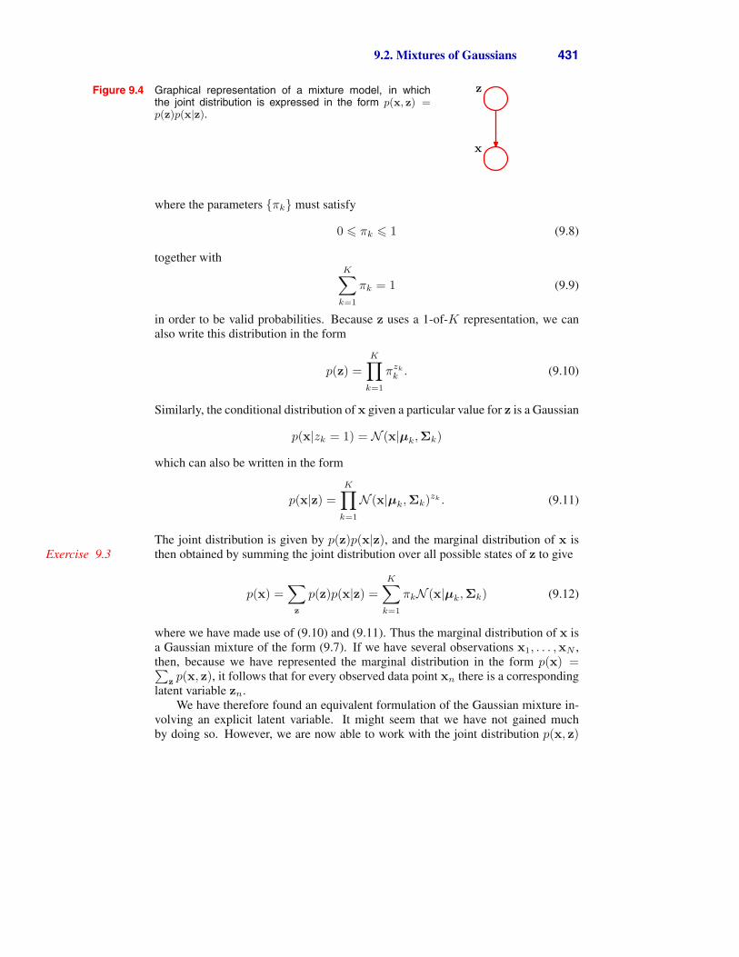
see that there are K possible states for the vector z according to which element isnonzero. We shall define the joint distribution p(x, z) in terms of a marginal dis-tribution p(z) and a conditional distribution p(x|z), corresponding to the graphicalmodel in Figure 9.4. The marginal distribution over z is specified in terms of themixing coefficients πk, such that

p(zk = 1) = πk

9.2. Mixtures of Gaussians 431

Figure 9.4 Graphical representation of a mixture model, in whichthe joint distribution is expressed in the form p(x, z) =p(z)p(x|z).

x

z

where the parameters {πk} must satisfy

0 � πk � 1 (9.8)

together withK�

k=1

πk = 1 (9.9)

in order to be valid probabilities. Because z uses a 1-of-K representation, we canalso write this distribution in the form

p(z) =K�

k=1

πzk

k . (9.10)

Similarly, the conditional distribution of x given a particular value for z is a Gaussian

p(x|zk = 1) = N (x|µk,Σk)

which can also be written in the form

p(x|z) =K�

k=1

N (x|µk,Σk)zk . (9.11)

The joint distribution is given by p(z)p(x|z), and the marginal distribution of x isthen obtained by summing the joint distribution over all possible states of z to giveExercise 9.3

p(x) =�

z

p(z)p(x|z) =K�

k=1

πkN (x|µk,Σk) (9.12)

where we have made use of (9.10) and (9.11). Thus the marginal distribution of x isa Gaussian mixture of the form (9.7). If we have several observations x1, . . . ,xN ,then, because we have represented the marginal distribution in the form p(x) =�

z p(x, z), it follows that for every observed data point xn there is a correspondinglatent variable zn.

We have therefore found an equivalent formulation of the Gaussian mixture in-volving an explicit latent variable. It might seem that we have not gained muchby doing so. However, we are now able to work with the joint distribution p(x, z)


instead of the marginal distribution p(x), and this will lead to significant simplifica-tions, most notably through the introduction of the expectation-maximization (EM)algorithm.

Another quantity that will play an important role is the conditional probabilityof z given x. We shall use γ(zk) to denote p(zk = 1|x), whose value can be foundusing Bayes’ theorem

γ(zk) ≡ p(zk = 1|x) =p(zk = 1)p(x|zk = 1)

K�

j=1

p(zj = 1)p(x|zj = 1)

=πkN (x|µk,Σk)

K�

j=1

πjN (x|µj ,Σj)

. (9.13)

We shall view πk as the prior probability of zk = 1, and the quantity γ(zk) as thecorresponding posterior probability once we have observed x. As we shall see later,γ(zk) can also be viewed as the responsibility that component k takes for ‘explain-ing’ the observation x.

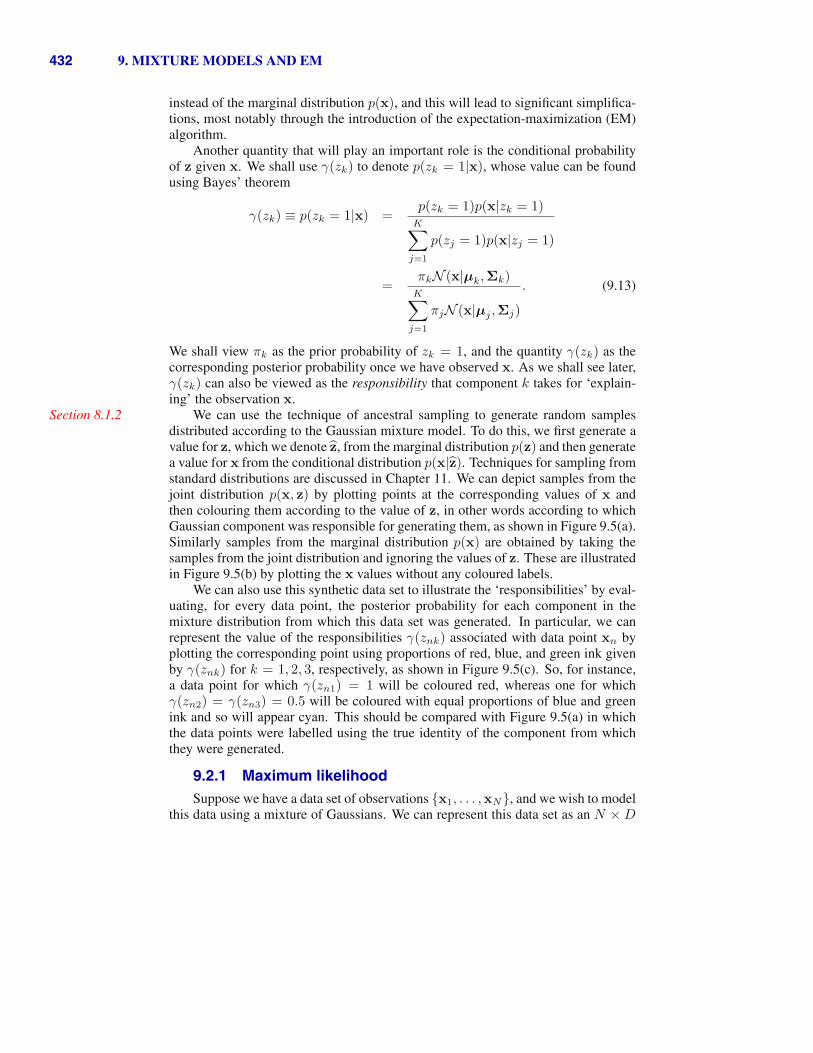
We can use the technique of ancestral sampling to generate random samplesSection 8.1.2distributed according to the Gaussian mixture model. To do this, we first generate avalue for z, which we denote �z, from the marginal distribution p(z) and then generatea value for x from the conditional distribution p(x|�z). Techniques for sampling fromstandard distributions are discussed in Chapter 11. We can depict samples from thejoint distribution p(x, z) by plotting points at the corresponding values of x andthen colouring them according to the value of z, in other words according to whichGaussian component was responsible for generating them, as shown in Figure 9.5(a).Similarly samples from the marginal distribution p(x) are obtained by taking thesamples from the joint distribution and ignoring the values of z. These are illustratedin Figure 9.5(b) by plotting the x values without any coloured labels.

We can also use this synthetic data set to illustrate the ‘responsibilities’ by eval-uating, for every data point, the posterior probability for each component in themixture distribution from which this data set was generated. In particular, we canrepresent the value of the responsibilities γ(znk) associated with data point xn byplotting the corresponding point using proportions of red, blue, and green ink givenby γ(znk) for k = 1, 2, 3, respectively, as shown in Figure 9.5(c). So, for instance,a data point for which γ(zn1) = 1 will be coloured red, whereas one for whichγ(zn2) = γ(zn3) = 0.5 will be coloured with equal proportions of blue and greenink and so will appear cyan. This should be compared with Figure 9.5(a) in whichthe data points were labelled using the true identity of the component from whichthey were generated.

9.2.1 Maximum likelihoodSuppose we have a data set of observations {x1, . . . ,xN}, and we wish to model

this data using a mixture of Gaussians. We can represent this data set as an N × D


(a)

0 0.5 1

0

0.5

1 (b)

0 0.5 1

0

0.5

1 (c)

0 0.5 1

0

0.5

1

Figure 9.5 Example of 500 points drawn from the mixture of 3 Gaussians shown in Figure 2.23. (a) Samplesfrom the joint distribution p(z)p(x|z) in which the three states of z, corresponding to the three components of themixture, are depicted in red, green, and blue, and (b) the corresponding samples from the marginal distributionp(x), which is obtained by simply ignoring the values of z and just plotting the x values. The data set in (a) issaid to be complete, whereas that in (b) is incomplete. (c) The same samples in which the colours represent thevalue of the responsibilities γ(znk) associated with data point xn, obtained by plotting the corresponding pointusing proportions of red, blue, and green ink given by γ(znk) for k = 1, 2, 3, respectively

matrix X in which the nth row is given by xTn . Similarly, the corresponding latent

variables will be denoted by an N × K matrix Z with rows zTn . If we assume that

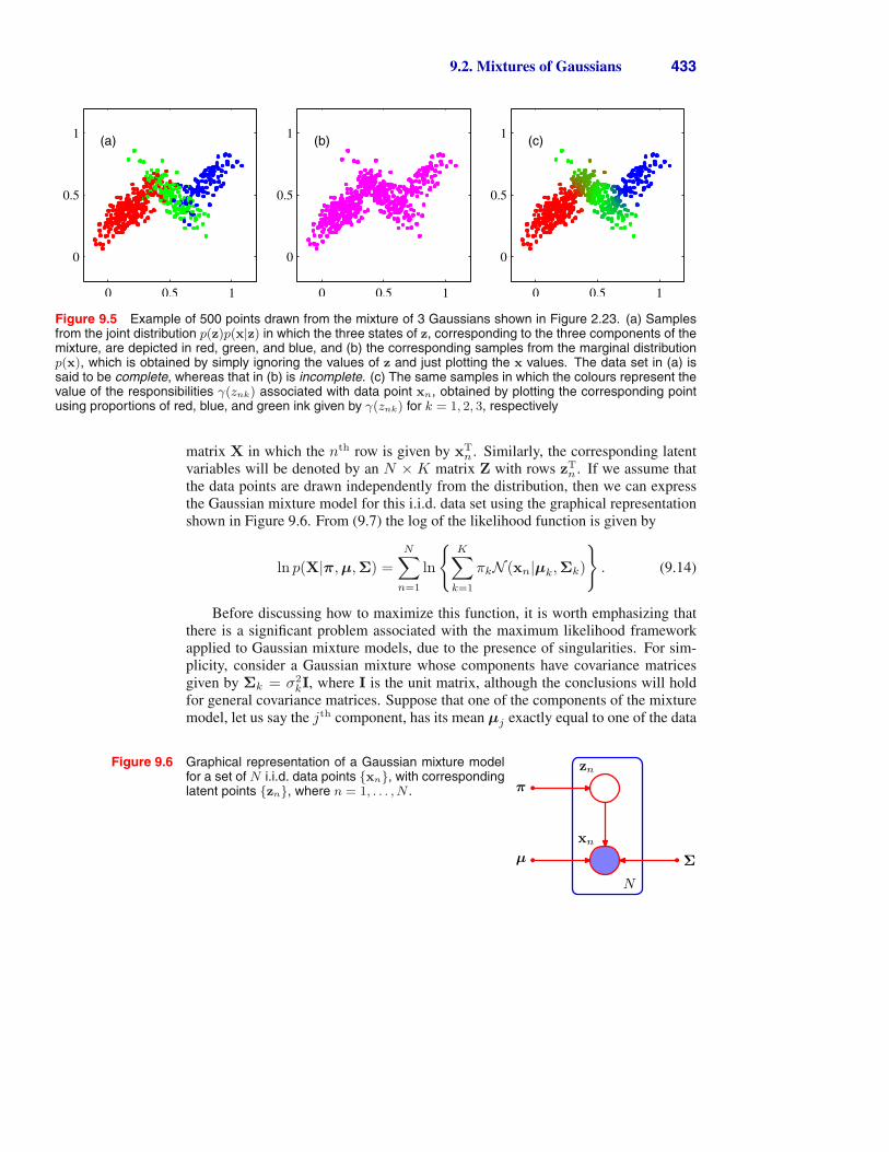
the data points are drawn independently from the distribution, then we can expressthe Gaussian mixture model for this i.i.d. data set using the graphical representationshown in Figure 9.6. From (9.7) the log of the likelihood function is given by

ln p(X|π, µ,Σ) =N�

n=1

ln

�K�

k=1

πkN (xn|µk,Σk)

�. (9.14)

Before discussing how to maximize this function, it is worth emphasizing thatthere is a significant problem associated with the maximum likelihood frameworkapplied to Gaussian mixture models, due to the presence of singularities. For sim-plicity, consider a Gaussian mixture whose components have covariance matricesgiven by Σk = σ2

kI, where I is the unit matrix, although the conclusions will holdfor general covariance matrices. Suppose that one of the components of the mixturemodel, let us say the jth component, has its mean µj exactly equal to one of the data

Figure 9.6 Graphical representation of a Gaussian mixture modelfor a set of N i.i.d. data points {xn}, with correspondinglatent points {zn}, where n = 1, . . . , N .

xn

zn

N

µ Σ

π


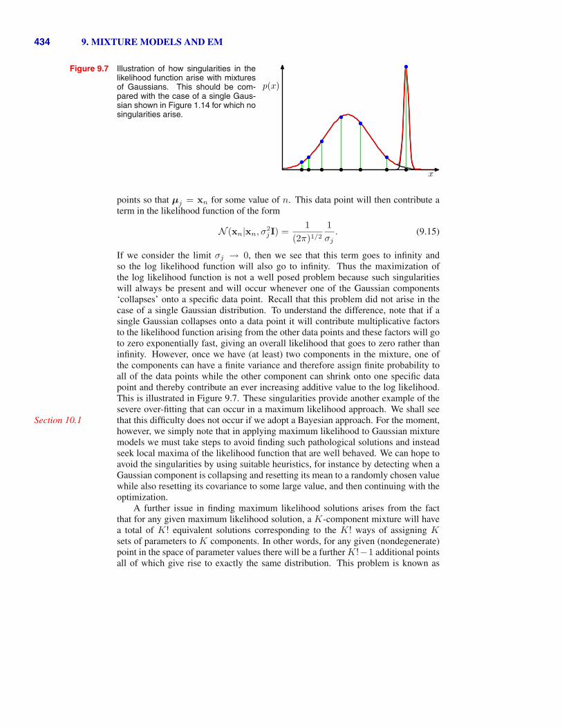
Figure 9.7 Illustration of how singularities in thelikelihood function arise with mixturesof Gaussians. This should be com-pared with the case of a single Gaus-sian shown in Figure 1.14 for which nosingularities arise.

x

p(x)

points so that µj = xn for some value of n. This data point will then contribute aterm in the likelihood function of the form

N (xn|xn, σ2j I) =

1(2π)1/2

1σj

. (9.15)

If we consider the limit σj → 0, then we see that this term goes to infinity andso the log likelihood function will also go to infinity. Thus the maximization ofthe log likelihood function is not a well posed problem because such singularitieswill always be present and will occur whenever one of the Gaussian components‘collapses’ onto a specific data point. Recall that this problem did not arise in thecase of a single Gaussian distribution. To understand the difference, note that if asingle Gaussian collapses onto a data point it will contribute multiplicative factorsto the likelihood function arising from the other data points and these factors will goto zero exponentially fast, giving an overall likelihood that goes to zero rather thaninfinity. However, once we have (at least) two components in the mixture, one ofthe components can have a finite variance and therefore assign finite probability toall of the data points while the other component can shrink onto one specific datapoint and thereby contribute an ever increasing additive value to the log likelihood.This is illustrated in Figure 9.7. These singularities provide another example of thesevere over-fitting that can occur in a maximum likelihood approach. We shall seethat this difficulty does not occur if we adopt a Bayesian approach. For the moment,Section 10.1however, we simply note that in applying maximum likelihood to Gaussian mixturemodels we must take steps to avoid finding such pathological solutions and insteadseek local maxima of the likelihood function that are well behaved. We can hope toavoid the singularities by using suitable heuristics, for instance by detecting when aGaussian component is collapsing and resetting its mean to a randomly chosen valuewhile also resetting its covariance to some large value, and then continuing with theoptimization.

A further issue in finding maximum likelihood solutions arises from the factthat for any given maximum likelihood solution, a K-component mixture will havea total of K! equivalent solutions corresponding to the K! ways of assigning Ksets of parameters to K components. In other words, for any given (nondegenerate)point in the space of parameter values there will be a further K!−1 additional pointsall of which give rise to exactly the same distribution. This problem is known as


identifiability (Casella and Berger, 2002) and is an important issue when we wish tointerpret the parameter values discovered by a model. Identifiability will also arisewhen we discuss models having continuous latent variables in Chapter 12. However,for the purposes of finding a good density model, it is irrelevant because any of theequivalent solutions is as good as any other.

Maximizing the log likelihood function (9.14) for a Gaussian mixture modelturns out to be a more complex problem than for the case of a single Gaussian. Thedifficulty arises from the presence of the summation over k that appears inside thelogarithm in (9.14), so that the logarithm function no longer acts directly on theGaussian. If we set the derivatives of the log likelihood to zero, we will no longerobtain a closed form solution, as we shall see shortly.

One approach is to apply gradient-based optimization techniques (Fletcher, 1987;Nocedal and Wright, 1999; Bishop and Nabney, 2008). Although gradient-basedtechniques are feasible, and indeed will play an important role when we discussmixture density networks in Chapter 5, we now consider an alternative approachknown as the EM algorithm which has broad applicability and which will lay thefoundations for a discussion of variational inference techniques in Chapter 10.

9.2.2 EM for Gaussian mixturesAn elegant and powerful method for finding maximum likelihood solutions for

models with latent variables is called the expectation-maximization algorithm, or EMalgorithm (Dempster et al., 1977; McLachlan and Krishnan, 1997). Later we shallgive a general treatment of EM, and we shall also show how EM can be generalizedto obtain the variational inference framework. Initially, we shall motivate the EMSection 10.1algorithm by giving a relatively informal treatment in the context of the Gaussianmixture model. We emphasize, however, that EM has broad applicability, and indeedit will be encountered in the context of a variety of different models in this book.

Let us begin by writing down the conditions that must be satisfied at a maximumof the likelihood function. Setting the derivatives of ln p(X|π, µ,Σ) in (9.14) withrespect to the means µk of the Gaussian components to zero, we obtain

0 = −N�

n=1

πkN (xn|µk,Σk)�j πjN (xn|µj ,Σj)� ��

γ(znk)

Σk(xn − µk) (9.16)

where we have made use of the form (2.43) for the Gaussian distribution. Note thatthe posterior probabilities, or responsibilities, given by (9.13) appear naturally onthe right-hand side. Multiplying by Σ−1

k (which we assume to be nonsingular) andrearranging we obtain

µk =1

Nk

N�

n=1

γ(znk)xn (9.17)

where we have defined

Nk =N�

n=1

γ(znk). (9.18)


We can interpret Nk as the effective number of points assigned to cluster k. Notecarefully the form of this solution. We see that the mean µk for the kth Gaussiancomponent is obtained by taking a weighted mean of all of the points in the data set,in which the weighting factor for data point xn is given by the posterior probabilityγ(znk) that component k was responsible for generating xn.

If we set the derivative of ln p(X|π, µ,Σ) with respect to Σk to zero, and followa similar line of reasoning, making use of the result for the maximum likelihoodsolution for the covariance matrix of a single Gaussian, we obtainSection 2.3.4

Σk =1

Nk

N�

n=1

γ(znk)(xn − µk)(xn − µk)T (9.19)

which has the same form as the corresponding result for a single Gaussian fitted tothe data set, but again with each data point weighted by the corresponding poste-rior probability and with the denominator given by the effective number of pointsassociated with the corresponding component.

Finally, we maximize ln p(X|π, µ,Σ) with respect to the mixing coefficientsπk. Here we must take account of the constraint (9.9), which requires the mixingcoefficients to sum to one. This can be achieved using a Lagrange multiplier andAppendix Emaximizing the following quantity

ln p(X|π, µ,Σ) + λ

�K�

k=1

πk − 1

�(9.20)

which gives

0 =N�

n=1

N (xn|µk,Σk)�j πjN (xn|µj ,Σj)

+ λ (9.21)

where again we see the appearance of the responsibilities. If we now multiply bothsides by πk and sum over k making use of the constraint (9.9), we find λ = −N .Using this to eliminate λ and rearranging we obtain

πk =Nk

N(9.22)

so that the mixing coefficient for the kth component is given by the average respon-sibility which that component takes for explaining the data points.

It is worth emphasizing that the results (9.17), (9.19), and (9.22) do not con-stitute a closed-form solution for the parameters of the mixture model because theresponsibilities γ(znk) depend on those parameters in a complex way through (9.13).However, these results do suggest a simple iterative scheme for finding a solution tothe maximum likelihood problem, which as we shall see turns out to be an instanceof the EM algorithm for the particular case of the Gaussian mixture model. Wefirst choose some initial values for the means, covariances, and mixing coefficients.Then we alternate between the following two updates that we shall call the E step


(a)−2 0 2

−2

0

2

(b)−2 0 2

−2

0

2

(c)

L = 1

−2 0 2

−2

0

2

(d)

L = 2

−2 0 2

−2

0

2

(e)

L = 5

−2 0 2

−2

0

2

(f)

L = 20

−2 0 2

−2

0

2

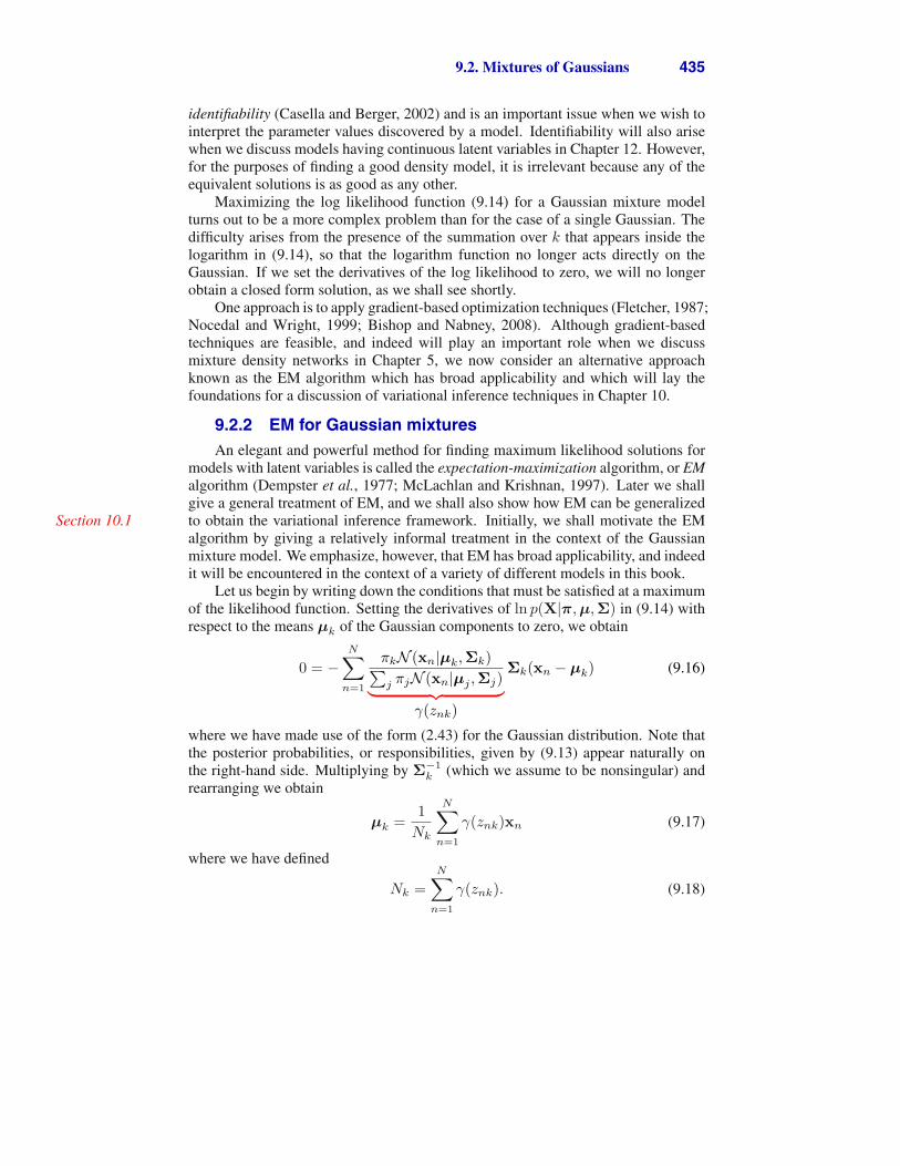
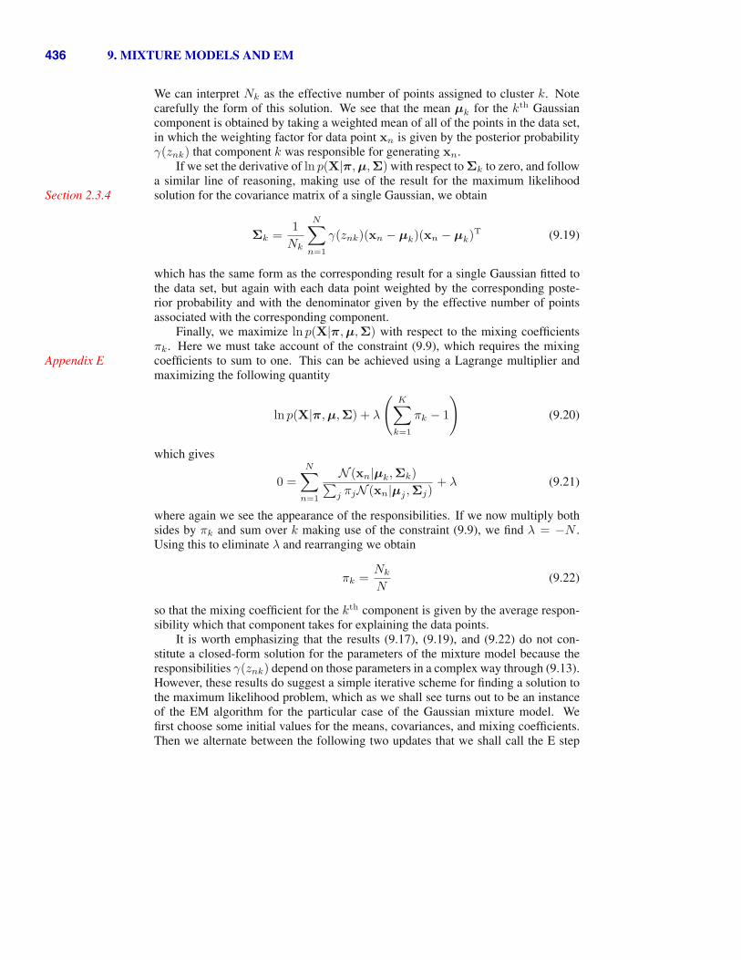
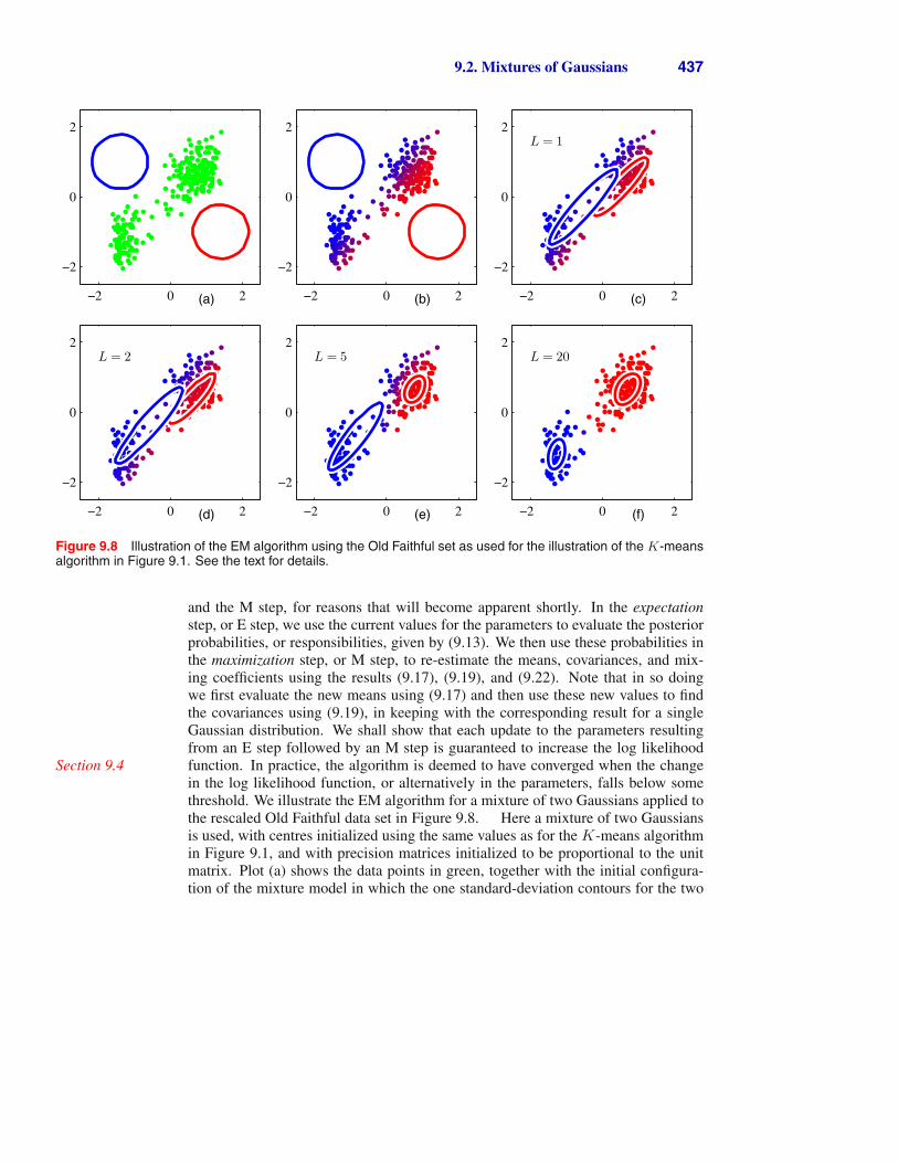
Figure 9.8 Illustration of the EM algorithm using the Old Faithful set as used for the illustration of the K-meansalgorithm in Figure 9.1. See the text for details.

and the M step, for reasons that will become apparent shortly. In the expectationstep, or E step, we use the current values for the parameters to evaluate the posteriorprobabilities, or responsibilities, given by (9.13). We then use these probabilities inthe maximization step, or M step, to re-estimate the means, covariances, and mix-ing coefficients using the results (9.17), (9.19), and (9.22). Note that in so doingwe first evaluate the new means using (9.17) and then use these new values to findthe covariances using (9.19), in keeping with the corresponding result for a singleGaussian distribution. We shall show that each update to the parameters resultingfrom an E step followed by an M step is guaranteed to increase the log likelihoodfunction. In practice, the algorithm is deemed to have converged when the changeSection 9.4in the log likelihood function, or alternatively in the parameters, falls below somethreshold. We illustrate the EM algorithm for a mixture of two Gaussians applied tothe rescaled Old Faithful data set in Figure 9.8. Here a mixture of two Gaussiansis used, with centres initialized using the same values as for the K-means algorithmin Figure 9.1, and with precision matrices initialized to be proportional to the unitmatrix. Plot (a) shows the data points in green, together with the initial configura-tion of the mixture model in which the one standard-deviation contours for the two


Gaussian components are shown as blue and red circles. Plot (b) shows the resultof the initial E step, in which each data point is depicted using a proportion of blueink equal to the posterior probability of having been generated from the blue com-ponent, and a corresponding proportion of red ink given by the posterior probabilityof having been generated by the red component. Thus, points that have a significantprobability for belonging to either cluster appear purple. The situation after the firstM step is shown in plot (c), in which the mean of the blue Gaussian has moved tothe mean of the data set, weighted by the probabilities of each data point belongingto the blue cluster, in other words it has moved to the centre of mass of the blue ink.Similarly, the covariance of the blue Gaussian is set equal to the covariance of theblue ink. Analogous results hold for the red component. Plots (d), (e), and (f) showthe results after 2, 5, and 20 complete cycles of EM, respectively. In plot (f) thealgorithm is close to convergence.

Note that the EM algorithm takes many more iterations to reach (approximate)convergence compared with the K-means algorithm, and that each cycle requiressignificantly more computation. It is therefore common to run the K-means algo-rithm in order to find a suitable initialization for a Gaussian mixture model that issubsequently adapted using EM. The covariance matrices can conveniently be ini-tialized to the sample covariances of the clusters found by the K-means algorithm,and the mixing coefficients can be set to the fractions of data points assigned to therespective clusters. As with gradient-based approaches for maximizing the log like-lihood, techniques must be employed to avoid singularities of the likelihood functionin which a Gaussian component collapses onto a particular data point. It should beemphasized that there will generally be multiple local maxima of the log likelihoodfunction, and that EM is not guaranteed to find the largest of these maxima. Becausethe EM algorithm for Gaussian mixtures plays such an important role, we summarizeit below.

EM for Gaussian Mixtures

Given a Gaussian mixture model, the goal is to maximize the likelihood functionwith respect to the parameters (comprising the means and covariances of thecomponents and the mixing coefficients).

1. Initialize the means µk, covariances Σk and mixing coefficients πk, andevaluate the initial value of the log likelihood.

2. E step. Evaluate the responsibilities using the current parameter values

γ(znk) =πkN (xn|µk,Σk)

K�

j=1

πjN (xn|µj ,Σj)

. (9.23)

9.3. An Alternative View of EM 439

3. M step. Re-estimate the parameters using the current responsibilities

µnewk =

1Nk

N�

n=1

γ(znk)xn (9.24)

Σnewk =

1Nk

N�

n=1

γ(znk) (xn − µnewk ) (xn − µnew

k )T (9.25)

πnewk =

Nk

N(9.26)

where

Nk =N�

n=1

γ(znk). (9.27)

4. Evaluate the log likelihood

ln p(X|µ,Σ, π) =N�

n=1

ln

�K�

k=1

πkN (xn|µk,Σk)

�(9.28)

and check for convergence of either the parameters or the log likelihood. Ifthe convergence criterion is not satisfied return to step 2.

9.3. An Alternative View of EM

In this section, we present a complementary view of the EM algorithm that recog-nizes the key role played by latent variables. We discuss this approach first of allin an abstract setting, and then for illustration we consider once again the case ofGaussian mixtures.

The goal of the EM algorithm is to find maximum likelihood solutions for mod-els having latent variables. We denote the set of all observed data by X, in which thenth row represents xT

n , and similarly we denote the set of all latent variables by Z,with a corresponding row zT

n . The set of all model parameters is denoted by θ, andso the log likelihood function is given by

ln p(X|θ) = ln

��

Z

p(X,Z|θ)

�. (9.29)

Note that our discussion will apply equally well to continuous latent variables simplyby replacing the sum over Z with an integral.

A key observation is that the summation over the latent variables appears insidethe logarithm. Even if the joint distribution p(X,Z|θ) belongs to the exponential

pattern recognition and machine learning - … · mixture models and em ... pattern recognition,...

Documents