1

Chapter 1

Pattern Recognition in Time Series

Jessica Lin Sheri Williamson Kirk Borne David DeBarr

George Mason University Microsoft Corporation

jessica@cs.gmu.edu swillif@gmu.edu kborne@gmu.edu dave.debarr@microsoft.com Abstract

Massive amount of time series data are generated daily, in areas as diverse as astronomy, industry, sciences, and aerospace, to name just a few. One obvious problem of handling time series databases concerns with its typically massive size—gigabytes or even terabytes are common, with more and more databases reaching the petabyte scale. Most classic data mining algorithms do not perform or scale well on time series data. The intrinsic structural characteristics of time series data such as the high dimensionality and feature correlation, combined with the measurement-induced noises that beset real-world time series data, pose challenges that render classic data mining algorithms ineffective and inefficient for time series. As a result, time series data mining has attracted enormous amount of attention in the past two decades.

In this chapter, we discuss the state-of-the-art techniques for time series pattern recognition, the process of mapping an input representation for an entity or relationship to an output category. Approaches to pattern recognition tasks vary by representation for the input data, similarity/distance measurement function, and pattern recognition technique. We will discuss the various pattern recognition techniques, representations, and similarity measures commonly used for time series. While the majority of work concentrated on univariate time series, we will also discuss the applications of some of the techniques on multivariate time series.

1. INTRODUCTION

Perhaps the most commonly encountered data type are time series, touching almost every aspect of human life, including astronomy. One obvious problem of handling time series databases concerns with its typically massive size—gigabytes or even terabytes are common, with more and more databases reaching the petabyte scale. For example, in telecommunication, large companies like AT&T produce several hundred millions long-distance records per day [Cort00]. In astronomy, time domain surveys are relatively new – these are surveys that cover a significant fraction of the sky with many repeat observations, thereby producing time series for millions or billions of objects. Several such time domain sky surveys are now completed, such as the MACHO [Alco01], OGLE [Szym05], SDSS Stripe 82 [Bram08], SuperMACHO [Garg08], and Berkeley’s Transients Classification Pipeline (TCP) [Star08] projects. The Pan-STARRS project is an active sky survey – it began in 2010, a 3-year survey covering three-fourths of the sky with ~60 observations of each field [Kais04]. The Large Synoptic Survey Telescope (LSST) project proposes to survey 50% of the visible sky repeatedly approximately 1000 times over a 10-year period, creating a 100-petabyte image archive and a 20-petabyte science database (http://www.lsst.org/). The LSST science database will include time series of over 100 scientific parameters for each of approximately 50 billion astronomical sources – this will be the largest data collection (and certainly the largest time series database) ever assembled in astronomy, and it rivals any

2

other discipline’s massive data collections for sheer size and complexity. More common in astronomy are time series of flux measurements. As a consequence of many

decades of observations (and in some cases, hundreds of years), a large variety of flux variations have been detected in astronomical objects, including periodic variations (e.g., pulsating stars, rotators, pulsars, eclipsing binaries, planetary transits), quasi-periodic variations (e.g., star spots, neutron star oscillations, active galactic nuclei), outburst events (e.g., accretion binaries, cataclysmic variable stars, symbiotic stars), transient events (e.g., gamma-ray bursts (GRB), flare stars, novae, supernovae (SNe)), stochastic variations (e.g., quasars, cosmic rays, luminous blue variables (LBVs)), and random events with precisely predictable patterns (e.g., microlensing events). Several such astrophysical phenomena are wavelength-specific cases, or were discovered as a result of wavelength-specific flux variations, such as soft gamma ray repeaters, X-ray binaries, radio pulsars, and gravitational waves. Despite the wealth of discoveries in this space of time variability, there is still a vast unexplored region, especially at low flux levels and short time scales (see also Bloom & Richards chapter in this book). Figure 1 illustrates the gap in astronomical knowledge in this time domain space. The LSST project aims to explore phenomena in the time gap.

Figure 1. Discovery space of astronomical variability. Numerous classes of flux variability have been identified through analysis of astronomical time series observations. But there is still a vast unexplored region of this parameter space that the LSST survey aims to explore. The axes on this plot are time scale of variability (abscissa) and the negative logarithm of the flux (ordinate), measured in magnitudes, where magnitudes decrease as an object gets brighter. This figure is reproduced from the LSST Science Book [Lsst09] and adapted from [Rau09].

In addition to flux-based time series, astronomical data also include motion-based time series. These include the trajectories of planets, comets, and asteroids in the Solar System, the motions of stars around the massive black hole at the center of the Milky Way galaxy, and the motion of gas filaments in the interstellar medium (e.g., expanding supernova blast wave shells). In most cases, the motions measured

3

in the time series correspond to the actual changing positions of the objects being studied. In other cases, the detected motions indirectly reflect other changes in the astronomical phenomenon, such as light echoes reflecting across vast gas and dust clouds, or propagating waves.

For concreteness, we define time series below:

Definition 1. Time Series: A time series T = t1,…,tm is an ordered set of m real-valued variables.

Figure 2 shows examples of time series data on several types of variable stars (reproduced from Rebbapragada et al. [Rebb09].

Figure 2. Examples of time series data for 3 different types of variable stars – the left panel in each case is the measured data, and the right panel is the processed data (including smoothing, interpolation, and spike removal). These data and processing results are reproduced from Rebbapragada et al. [Rebb09].

Most classic data mining algorithms do not perform or scale well on time series data. The intrinsic

structural characteristics of time series data such as the high dimensionality and feature correlation, combined with the measurement-induced noises that beset real-world time series data, pose challenges

4

that render classic data mining algorithms ineffective and inefficient for time series. As a result, time series data mining has attracted enormous amount of attention in the past two decades. Some of the areas that have seen the majority of research in time series data mining include indexing (query by content) [Agra93, Agra95, Came10, Chan99, Chen05, Ding08, Falo94, Keog01, Keog02b, Lin07, Yi00], clustering [Kalp01, Keog98, Keog04, Liao05, Lin04], classification [Geur01, Rado10, Wei06], anomaly detection [Dasg99, Keog02c, Keog05, Pres09, Yank08], and motif discovery [Cast10, Chiu03, Lin02, Minn06, Minn07, Muee09, Muee10, Tang08]. All tasks require that the notion of similarity be defined. As a result, similarity search has been an active research area in the last two decades.

In all of the above astronomical cases, pattern recognition and mining of the time series data falls into the usual three categories: supervised learning (classification), unsupervised learning (pattern detection, clustering, class discovery, characterization, change detection, and Fourier, wavelet, or principal component decomposition), and semi-supervised learning (semi-supervised classification, outlier/surprise/novelty/anomaly detection). For each of these applications, scientific knowledge discovery is the goal. Approaches to pattern recognition tasks vary by representation for the input data, similarity/distance measurement function, and pattern recognition technique. In this chapter, we discuss the various supervised, semi-supervised, and unsupervised learning techniques, representations, and similarity measures commonly used for time series. While the majority of work concentrated on univariate time series, we will also discuss the applications of some of the techniques on multivariate time series.

2. Pattern Recognition Approaches

Previous work on time series pattern recognition focuses on one of the three areas: pattern recognition algorithms, efficient time series representations and dimensionality reduction techniques, and similarity measures for time series data.

2.1 Pattern Recognition Algorithms Pattern recognition is the process of automatically mapping an input representation for an entity or

relationship to an output category. The recognition task is generally categorized based on how the learning procedure determines the output category. The learning procedure can be supervised (when a given pattern is assigned to one of the pre-defined classes, using labeled data to build a model or guide the pattern classification), unsupervised (when a given pattern is assigned to an unknown class), or semi-supervised (when a given pattern is assigned to one of the pre-defined classes, using both labeled and unlabeled data). For supervised learning, or classification, a functional model is often used to map observed inputs to output categories. A great deal of model construction techniques have been developed for this purpose [Duda00], including decision trees, rule induction, Bayesian networks, memory-based reasoning, Support Vector Machines (SVMs), and neural networks.

Memory-based reasoning methods, such as nearest neighbor, have been successfully used for classification of time series data. The Nearest Neighbor (NN) classification algorithm works by computing the distance between the object to be classified and each member of the training set [Han00]. The classification of the object to be classified is predicted to be the same as the classification of the nearest training set member. A common variation of this algorithm predicts the classification of the test object to be the most common classification found among the “k” nearest neighbors in the training set (k-NN). The 1-NN classifier, with leaving-one-out cross validation, has become the standard method used to compare and evaluate the utilities of time series representations and similarity measures [Ding08].

Another common choice of classifier is decision tree. A decision tree [Han00] is classic machine learning tool that uses a flow-chart-like tree structure, in which an internal node denotes a test on an attribute, a branch denotes the outcome on a test, and a leaf node denotes the class label or class distribution. By placing the attribute that best distinguishes the data (i.e. the one resulting in the highest information gain) at the root, a decision tree induction process recursively partitions the data samples into

5

subsets of samples based on the attribute splitting criterion. The resulting tree can be used to classify future incoming samples, and it can also be easily converted to a set of rules that generalize the behaviors of the data. While decision trees are defined for real data, attempting to classify time series using the raw data would clearly be a mistake, since the high dimensionality and noise levels would result in a deep, bushy tree with poor accuracy [Lin07]. In an attempt to overcome this problem, Geurts [Geur01] suggested representing the time series as a Regression Tree (RT), and training the decision tree directly on this representation. The technique shows great promise.

Support Vector Machines (SVMs) [Duda00, Rodr05] are commonly used for constructing classification models for high-dimensional representations. The observations from the training set which best define the decision boundary between classes are chosen as support vectors (they support/define the decision boundary). A non-zero weight is assigned to each support vector. The classification of a test object is predicted by computing a weighted sum of similarity function output between the new object and the support vectors for each class. The predicted class is the class with the largest sum, relative to a bias (offset) for the decision boundary. Kernel functions are used to measure the similarity between objects. Common kernel functions for this purpose include the cosine similarity function and the Gaussian RBF. SVMs have been used for time series classification by several researchers. Chaovalitwongse and Pardalos used SVMs with dynamic time warping kernel for brain activity classification [Chao08]. Kampouraki et al. [Kamp09] extracted features from ECG time series using statistical methods and signal analysis techniques, and classified the data using SVMs. Eads et al. proposed to use genetic algorithms to extract time series features, which are then classified using SVMs [Eads02].

Artificial Neural Networks (ANN) [Lipp87], also known as neural networks or neural nets, are analogous to their namesake, biological neural networks, in that both receive multiple inputs and respond with a single output. ANNs are comprised of connected nodes, called neurons, which are partitioned into layers. Networks may contain an input layer, an output layer, and a hidden inner layer, and additional hidden layers may be added to increase the complexity of the network. Weights are assigned to each of the links between neurons, and they are updated as part of the learning process. A simple example of an ANN is a perceptron [Rose58], which is a two-class linear classifier that is composed of a single-layered neural network. During training, each example is fed through the network, and the weights are updated according to the difference between the actual and expected output. During testing, the weighted sum of the network (the dot product of the instance and the vector of weights) is compared to a bias parameter to classify each instance as either a positive or negative instance. ANNs generalize well to previously unseen instances because they map every possible input to some output. Additionally, they are robust because even if a node is faulty or is removed, since the work is distributed across the network, it is still possible to achieve good results. ANNs have been successfully applied to domains such as character recognition [Desa10], face detection [Aitk03], intrusion detection [Amin06], speech recognition [Dede10], autonomous driving [Pome89], and astronomy [Coll04, Wang09]. In recent years, research has shown that constructing an ensemble of neural networks, where the majority vote determines the classification, can improve the accuracy of ANNs [Kim07, Kras07, Mink08, Zhou02].

Semi-Supervised Learning All of the techniques described above are supervised learning techniques, for which training

examples with known classification labels are used to construct a model to label test examples with unknown classification labels. Semi-supervised learning on the other hand involves using both the training examples with known classification labels and the test examples with unknown classification labels to construct a model to label the examples with unknown classification labels. While it’s possible to construct a model for labeling future test examples, it’s also possible to construct a model that focuses on the current test examples. Vapnik referred to this as transduction [Vapn98], suggesting that it’s better to focus on the simpler problem of classifying the current test examples rather than trying to construct a model to future test examples. For time series, Wei and Keogh [Wei06] proposed a semi-supervised classification technique based on 1-NN. The algorithm starts by training the classifier using all labeled

6

data. It then classifies unlabeled data, and adds the most confidently classified unlabeled data into the training set [Wei06]. This process is repeated until some stopping criterion is reached. This algorithm is an example of self-training algorithms [Zhu05]. The authors have shown that their algorithm requires only a handful of labeled data to construct an accurate classifier.

In addition to semi-supervised classification, semi-supervised learning is also applicable to anomaly detection and novelty discovery, since we often do not know what’s anomalous in advance. In fact, anomaly detection is often regarded as a binary classification problem. A simple idea for detecting anomalous behavior in time series is to examine previously observed normal data and build a model of it. Data obtained in the future can be compared to this model and any lack of conformity can signal an anomaly [Das99]. In order to achieve this, Keogh et al combined a statistically sound scheme with an efficient combinatorial approach [Keog02c]. The statistically scheme is based on Markov chains and normalization. Markov chains are used to model the “normal” behavior, which is inferred from the previously observed data. The time- and space-efficiency of the algorithm comes from the use of a suffix tree as the main data structure. Each node of the suffix tree represents a pattern. The tree is annotated with a score obtained comparing the support of a pattern observed in the new data with the support recorded in the Markov model. Model-free anomaly detection approaches have also been proposed. In a previous work, we defined time series discords to be subsequences of a longer time series that are maximally different from all the rest of the subsequences [Keog06b]. They thus capture the sense of the most unusual subsequence within a time series. Time series discords are superlative anomaly detectors, able to detect subtle anomalies in diverse domains. In fact, in a recent extensive empirical study, Vipin Kumar concluded “..on 19 different publicly available data sets, comparing 9 different techniques time series discord is the best overall technique among all techniques” [Chan09].

Unsupervised Learning Unlike supervised or semi-supervised learning, unsupervised learning (e.g. clustering) involves only

unlabeled data. One of the most widely used clustering approaches is hierarchical clustering, due to the great visualization power it offers [Keog98]. Hierarchical clustering produces a nested hierarchy of similar groups of objects, according to a pairwise distance matrix of the objects. One of the advantages of this method is its generality, since the user does not need to provide any parameters such as the number of clusters. However, its application is limited to only small datasets, due to its quadratic (or higher order) computational complexity.

A faster method to perform clustering is k-Means [McQu67, Brad98]. Table 1 summarizes the algorithm.

Table 1. An outline of the k-Means algorithm

Algorithm k-Means

1 Decide on a value for k.

2 Initialize the k cluster centers (randomly, if necessary).

3 Decide the class memberships of the N objects by assigning them to the nearest cluster center.

4 Re-estimate the k cluster centers, by assuming the memberships found above are correct.

5 If none of the N objects changed membership in the last iteration, exit. Otherwise goto 3.

The basic intuition behind k-Means (and in general, iterative refinement algorithms) is the

continuous reassignment of objects into different clusters, so that the within-cluster distance is minimized. Therefore, if x are the objects and c are the cluster centers, k-Means attempts to minimize the following objective function:

7

∑∑= =

−=k

m

N

imi cxF

1 1 (1)

The k-Means algorithm for N objects has a complexity of O(kNrD) [McQu67], where k is the number of clusters specified by the user, r is the number of iterations until convergence, and D is the dimensionality of the points. The shortcomings of the algorithm are its tendency to favor spherical clusters, and its requirement for prior knowledge on the number of clusters, k. The latter limitation can be mitigated by attempting all values of k within a large range. Various statistical tests can then be used to determine which value of k is most parsimonious. Since k-Means is essentiality a hill-climbing algorithm, it is guaranteed to converge on a local but not necessarily global optimum. In other words, the choices of the initial centers are critical to the quality of results. Nevertheless, in spite of these undesirable properties, for clustering large datasets of time-series, k-Means is preferable due to its faster running time.

Another well-known partitional clustering algorithm is the EM (Expectation-Maximization) algorithm. The EM algorithm with Gaussian Mixtures is very similar to k-Means. As with k-Means, the algorithm begins with an initial guess as to the location of the clusters. The steps are: (1) the data are apportioned into separate localized data elements weighted according to the cluster models (the "E" step); and then (2) the parameters of the cluster models (location, width, etc.) are fit to these data elements by maximizing some goodness-of-fit quantity (the "M" step); (3) steps (1) and (2) are repeated until the model converges. In some cases convergence is slow or otherwise problematic.

The major distinction between EM and k-Means is that k-Means attempts to model the data as a collection of k spherical regions, with every data object belonging to exactly one cluster. In contrast, EM models the data as a collection of k Gaussians, with every data object having some degree of membership in each cluster (in fact, although Gaussian models are most common, other distributions are possible). The major advantage of EM over k-Means is its ability to model a much richer set of cluster shapes. This generality has made EM (and its many variants and extensions) the clustering algorithm of choice in data mining [Demp77] and bioinformatics [Lawr90].

Specialized clustering algorithms have been proposed for time series. For example, Lin et al [Lin04] proposed an incremental and iterative version of the k-Means algorithm called i-kMeans. The algorithm works by leveraging off the multi-resolution property of wavelets, which mitigates the dilemma of initial centers selection for k-Means [Lin04]. They further extended the approach to a general framework, which works for any iterative refining clustering algorithms (such as EM), with any multi-resolution decomposition methods. Rodriguez et al [Rodr06] proposed a hierarchical clustering algorithm for time series data streams. The algorithm incrementally constructs a tree-like hierarchy of clusters, using a correlation-based dissimilarity measure between time series [Rodr06]. 2.2 Time Series Representations and Symbolic Aggregate approXimation (SAX)

With the rapid growth of storage technology, datasets from practical applications typically do not fit in main memory, and disk I/O tends to be the bottleneck for any data mining task. The sheer volume of time series databases makes sequential scanning of the databases infeasible for any data mining and retrieval tasks. A simple generic framework for time series data mining has thus emerged [Lin07]. It works by (1) approximating the time series data with some representation that typically fits in the main memory, (2) approximately solving the problem at hand using the representation, and (3) validating the results by making (hopefully) a small number of disk accesses.

It is obvious that the quality of the framework heavily relies on the quality of the representation. If the representation is faithful to the original data, then the approximate solutions obtained from Step 2 will be close to the actual solutions. Towards this end, many high-level time series representations have been proposed, including Discrete Fourier Transform (DFT) [Agra93], Discrete Wavelet Transform (DWT) [Chan99], Piecewise Linear Aggregate (PLA) and Piecewise Constant models (PAA) [Keog01], and Adaptive Piecewise Constant Approximation (APCA) [Keog01]. Figure 3 illustrates a hierarchy of the various representations in the literature.

8

Figure 3. A hierarchy of all the various time series representations in the literature.

These representations allow fast access to the “approximation” version of the data via some index

structure, so as to relieve the burden associated with disk I/Os. In addition, since time series data are typically very high dimensional and noisy, it is essential to reduce its dimensionality via one of these representations. In fact, even though most of the representations use only a few coefficients to represent the data, they often result in better accuracy than the raw data due to the implicit noise removal.

One important feature of most of the representations is that they are real valued. This limits the algorithms, data structures and definitions available for them. Such limitations have led researchers to consider using a symbolic representation for time series. In addition, there is an enormous wealth of existing algorithms and data structures that allow the efficient manipulations of strings, e.g. hashing, Markov models, suffix trees, decision trees etc. Such algorithms have received decades of attention in the text retrieval community, and more recent attention from the bioinformatics community.

While many symbolic representations of time series have been introduced over the past decades, they suffer from two fatal flaws: (1) The dimensionality of the symbolic representation is the same as the original data, and virtually all data mining and indexing algorithms degrade exponentially with dimensionality. (2) Although distance measures can be defined on the symbolic approaches, these distance measures have little correlation with distance measures defined on the original signals. In our previous work, we introduced a symbolic representation for time series called Symbolic Aggregate approXimation (SAX) [Lin07] that remedies the problems mentioned above. More specifically, SAX is both time- and space-efficient, and we can define a distance measure that guarantees the distance between two SAX strings to be no larger than the true distance between the original time series. This lower-bounding property is at the core of almost all algorithms in time series data mining [Falo94]. It plays an important role in indexing and similarity search, since it’s the essential key to guarantee no false dismissal of results. In general, without a lower-bounding distance measure, one cannot meaningfully compute the approximate solution in the representation space, since the approximate solution obtained may be arbitrarily dissimilar to the true solution obtained from the original data.

SAX performs the discretization by dividing a time series into w equal-sized segments. For each segment, the mean value for the points within that segment is computed. Aggregating these w coefficients forms the Piecewise Aggregate Approximation (PAA) representation of T. Each coefficient is then mapped to a symbol according to a set of breakpoints that divide the distribution space into α equiprobable regions, where α is the alphabet size specified by the user. If the symbols were not equiprobable, some of the symbols would occur more frequently than others. As a consequence, we would inject a probabilistic bias in the process. It has been noted that some data structures such as suffix trees produce optimal results when the symbols are of equiprobability [Croc94]. The discretization steps are summarized in Figure 4.

9

Figure 4: A time series is discretized by first obtaining a PAA approximation and then using predetermined breakpoints to map the PAA coefficients into SAX symbols. In the example above, with n = 128, w = 8 and a = 3, the time series is mapped to the word baabccbc

Preliminary results show that SAX is competitive compared to other time series representations

[Lin07]. SAX has had a large impact in both industry and academia. It has received a large number of references, and it has been used worldwide in many domains1. To name a few, Chen et al. convert palmprint to time series, then to SAX, and then perform biometric recognition [Chen05b]. Murakami et al. use SAX to find repeated patterns in robot sensors [Mura04]. Pouget et al. use SAX for the detection of multi-headed stealthy attack tools [Poug06]. McGovern et al. use SAX for the prediction of severe weather phenomena such as tornados, thunderstorms, hail, and floods [McGo10].

Many researchers have introduced various time series data mining algorithms that use SAX as a representation. For example, Bakalov et al. use SAX to do spatiotemporal trajectory joins [Baka05]. Many motif discovery [Cast10, Chiu03, Lin02, Minn06, Minn07, Muee09, Muee10, Tang08] and anomaly detection [Dasg99, Keog02c, Keog05, Pres09, Yank08] algorithms have been proposed that utilize SAX as the representation.

While there have been dozens of applications of SAX to diverse problems, there has been surprisingly little work to augment or extend the SAX representation itself. We attribute this to the generality of the original framework; it simply works very well for most problems. Nevertheless, there have been some SAX extensions, which we consider below. Lkhagva et al. augment each SAX symbol by incorporating the minimum and maximum value in the range [Lkha06]. Thus each SAX segment contains a triplet of information, rather than a single symbol. Very preliminary results are presented which suggest that this may be useful in some domains. Bernard Hugueney [Hugu06] has recently suggested that SAX could be improved by allowing SAX symbols to adaptively represent different length sections of a time series. Just as SAX may be seen as symbolic a symbolic version of the PAA representation, Dr. Hugueneys approach may be seen as a symbolic version of the APCA representation [Keog01]. In contrast to Hugueneys idea of allowing segment lengths to be adaptive, work by Morchen and Ultsch has suggested that the breakpoints should be adaptive [Morc05]. The authors make a convincing case that in some datasets this may be better than the Gaussian assumption. Shieh and Keogh introduced iSAX [Shie08], the generalization of SAX that allows multiresolution indexing and mining of massive time series data.

To see how SAX compares to Euclidean distance, we ran an extensive 1-NN classification experiment and compared the error rates on 22 publicly available datasets2 [Lin07]. Each dataset is split to training and testing parts. We use the training part to search the best value for SAX parameters w (number of SAX words) and a (size of the alphabet):

• For w, we search from 2 up to n/2 (n is the length of the time series). Each time we double the value of w.

• For a, we search each value between 3 and 10.

1 For a more complete list of papers that extend and use SAX, see http://www.cs.gmu.edu/~jessica/sax.htm 2 Available online at http://www.cs.ucr.edu/~eamonn/time_series_data/

10

• If there is a tie, we use the smaller values.

The compression ratio (last column of next table) is calculated as: , because for SAX

representation we only need bits per word, while for the original time series we need 4 bytes (32 bits) for each value.

Then we classify the testing set based on the training set using one nearest neighbor classifier and report the error rate. The results are shown in Table 1 [Lin07]. From this experiment, we can conclude that SAX is competitive with Euclidean distance, but requires far less space. More experiments that compare different time series representations can be found in [Ding08].

Table 1. 1-NN classification results between SAX and raw data using Euclidean Distance Name Number

of Classes

Size of Training

Set

Size of Testing Set

Time Series Length

1-NN EU Error

1-NN SAX Error

w a Compression Ratio

Synthetic Control

6 300 300 60 0.12 0.02 16 10 3.33%

Gun-Point 2 50 150 150 0.087 0.18 64 10 5.33% CBF 3 30 900 128 0.148 0.104 32 10 3.13% Face (all) 14 560 1690 131 0.286 0.330 64 10 6.11% OSU Leaf 6 200 242 427 0.483 0.467 128 10 3.75% Swedish Leaf 15 500 625 128 0.211 0.483 32 10 3.13% 50Words 50 450 455 270 0.369 0.341 128 10 5.93% Trace 4 100 100 275 0.24 0.46 128 10 5.82% Two Patterns 4 1000 4000 128 0.093 0.081 32 10 3.13% Wafer 2 1000 6174 152 0.0045 0.0034 64 10 5.26% Face (four) 4 24 88 350 0.216 0.170 128 10 4.57% lightning-2 2 60 61 637 0.246 0.213 256 10 5.02% lightning-7 7 70 73 319 0.425 0.397 128 10 5.02% ECG 2 100 100 96 0.12 0.12 32 10 4.17% Adiac 37 390 391 176 0.389 0.890 64 10 4.55% Yoga 2 300 3000 426 0.170 0.195 128 10 3.76% Fish 7 175 175 463 0.217 0.474 128 10 3.46% Plane 7 105 105 144 0.038 0.038 64 10 5.56% Car 4 60 60 577 0.267 0.333 256 10 5.55% Beef 5 30 30 470 0.467 0.567 128 10 3.40% Coffee 2 28 28 286 0.25 0.464 128 10 5.59% Olive Oil 4 30 30 570 0.133 0.833 256 10 5.61%

2.3 Similarity Measure Another active area of research in time series data mining is similarity measure, since all tasks,

including classification and clustering, require that the notion of similarity be defined. As a result, many distance/similarity measures have been proposed for time series data. We start by defining Dist(A, B), the distance between two objects A and B.

Definition 2. Distance: Dist is a function that has two objects A and B as inputs and returns a nonnegative value R, which is said to be the distance from A to B.

Each time series is normalized to have a mean of zero and a standard deviation of one before calling

⎡ ⎤32log2×

×

naw

⎡ ⎤a2log

11

the distance function, since it is well understood that in virtually all settings, it is meaningless to compare time series with different offsets and amplitudes [Keog02]. It should be noted that not all similarity measures are distance metrics. For a function calculating the similarity/dissimilarity between the time series A and B to qualify as a distance metric, it must satisfy the following conditions [Keog04b]:

1. Symmetry D(A,B) = D(B,A) 2. Constancy D(A,A) = 0 3. Positivity D(A,B) = 0 if and only if A = B 4. Triangle Inequality D(A,B) <= D(A,C) + D(B,C)

If a similarity measure satisfies the requirements to be a distance metric, then it can be used to index the time series in a database, which makes queries (e.g. searching for the nearest neighbor) more efficient.

Similarity measures can be categorized, based on how features are extracted and how similarity is determined, into shape-based similarity and structure-based similarity. The former determines the similarity of two time series by comparing their individual point values, whereas the latter looks at the higher-level structures. We discuss the two kinds of similarity in more details in the following sections. 2.3.1 Shape-Based Similarity

Given two time series Q and C, their shape-based similarity can be determined by comparing local point values. By far the most common distance measure for time series is the Euclidean distance. Assuming that Q and C are of the same length n, Eq. 2 defines their Euclidean distance.

(2)

The simplicity and efficiency of Euclidean distance makes it the most popular distance measure in data mining, and it has the advantage of being a distance metric. However, a major drawback for Euclidean distance is that it is very brittle. It requires that both input sequences be of the same length, and it is sensitive to distortions, e.g. shifting, along the time axis. Such a problem can generally be handled by elastic distance measures such as Dynamic Time Warping (DTW) [Keogh02b] and Longest Common SubSequence (LCSS) [Vlac02].

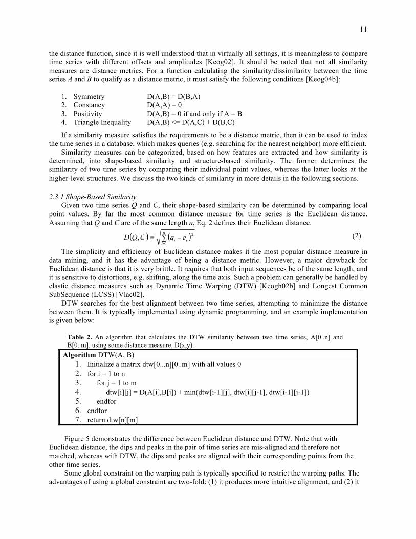
DTW searches for the best alignment between two time series, attempting to minimize the distance between them. It is typically implemented using dynamic programming, and an example implementation is given below:

Table 2. An algorithm that calculates the DTW similarity between two time series, A[0..n] and B[0..m], using some distance measure, D(x,y).

Algorithm DTW(A, B) 1. Initialize a matrix dtw[0...n][0..m] with all values 0 2. for i = 1 to n 3. for j = 1 to m 4. dtw[i][j] = D(A[i],B[j]) + min(dtw[i-1][j], dtw[i][j-1], dtw[i-1][j-1]) 5. endfor 6. endfor 7. return dtw[n][m]

Figure 5 demonstrates the difference between Euclidean distance and DTW. Note that with

Euclidean distance, the dips and peaks in the pair of time series are mis-aligned and therefore not matched, whereas with DTW, the dips and peaks are aligned with their corresponding points from the other time series.

Some global constraint on the warping path is typically specified to restrict the warping paths. The advantages of using a global constraint are two-fold: (1) it produces more intuitive alignment, and (2) it

( ) ( )∑ −≡=

n

iii cqCQD

1

2,

12

speeds up the computation by narrowing the search space. A large warping window causes the search to become prohibitively expensive, as well as possibly allowing meaningless matching between points that are far apart. On the other hand, a small window might prevent us from finding the best solution. It has been shown by Ratanamahatana and Keogh [Rata04] that by learning the best size and shape of the global constraint for different datasets, higher accuracy can be achieved.

While DTW is a more robust distance measure than Euclidean Distance, it is also a lot more computationally intensive than Euclidean Distance, even with the presence of a global constraint. Keogh proposed an indexing scheme for DTW that allows faster retrieval [Keog02b]. Nevertheless, DTW is still at least several orders slower than Euclidean distance.

Figure 5. (Left) Alignment for Euclidean distance between two sequence data. (Right) Alignment for Dynamic Time Warping distance between two sequence data.

Notice that DTW requires a distance measure for comparing two observations, one from each time

series; typically the L1 or L2 norm is used. LCSS, as its name suggests, finds the length of the longest matching subsequence. Originally created

for discrete values, it can be adapted to continuous values in time series by redefining a “match” to be whenever the difference between two observations in the time series is below a given threshold. Also typically implemented using dynamic programming, the algorithm is given below:

Table 3. An algorithm that calculates the LCSS between two time series, A[0..n] and B[0..m], using some distance measure, D(x,y), and a threshold, δ.

Algorithm LCSS(A, B) 1. Initialize a matrix lcss[0...n][0..m] with all values 0 2. for i = 1 to n 3. for j = 1 to m 4. if (D(A[i],B[j]) < δ) 5. lcss[i][j] = lcss[i-1][j-1] + 1 6. else 7. lcss[i][j] = max(lcss[i][j-1], lcss[i-1,j]) 8. endif 9. endfor 10. endfor 11. return 1 - lcss[n][m] / min(n,m)

Compared to Euclidean distance, DTW and LCSS are more elastic, supporting local time shifts and

variations in lengths of pairs of time series, but they are also more expensive to compute. Of the three measures, LCSS is the least sensitive to noise because it includes a threshold to define a “match.”

Note that the above definition of LCSS works well for univariate time series, where there are observations through time of only one variable. However, multivariate time series can encounter a situation where one threshold does not hold well across all variables. Thus, we introduce a variation on LCSS, which we call LCSS Relaxed, in our experimental results. In this variation, to constitute a “match” for multivariate time series, only a percentage of variables must “match” according to the given

13

threshold. Since DTW and LCSS do not satisfy the triangle inequality, they are not distance metrics. Other

elastic distance metrics such as Edit distance with Real Penalty (ERP) [Chen04] and Time-Warp Edit Distance (TWED) [Mart09] have been proposed. Both ERP and TWED have their roots in the classic string edit distance, which calculates the minimum number of insertions, deletions, and substitutions required to transform one string into another. ERP calls an inserted or deleted element to be a ‘gap’ in the opposing time series and it defines a constant, g, to use in calculating the penalty for gaps.

Given two time series, A[0..n] and B[0..m], and a constant g, ERP is determined by using Eq. 3 as the recursive formula for dynamic programming.

(3)

A feature of particular interest for TWED is that it can account for time stamp differences between each observation. That is, each observation in the time series is taken at a different moment in time, and while other measures assume observations were taken at a consistent sampling rate, TWED can account for inconsistent observations. This makes it possible to compare time series with irregular or inconsistent sampling rates or missing values. In addition to using a similar gap penalty as ERP, TWED also defines a constant, λ, which controls the stiffness of elastic matching.

Using dynamic programming, TWED is determined by Eq. 4, where Dist is a distance measure (e.g. Dist(a, b) = | a – b | + λ | ta – tb | , where ti is the timestamp for observing instance i in time series I)

(4) Experimental Results. Several studies that compare time series similarity measures have been performed [Ding08, Keog02, Keog06a]. Most of them focus on univariate time series. In this chapter, we compare the various similarity measures discussed above on multivariate time series classification. Five time series datasets were chosen, and Table 4 shows the characteristics of the datasets.

Table 4. Important Features of Datasets

AUSLAN3 Japanese Vowels4

Wafer5 ECG6 Star Light Curve7

3 M. Kadous. Australian Sign Language Signs (High Quality) Data Set. The UCI KDD Archive, 26 February 2002. http://archive.ics.uci.edu/ml/databases/auslan2/ 4 M. Kudo, J. Toyama, M. Shimbo. Japanese Vowels. The UCI KDD Archive, 13 June 2000. http://archive.ics.uci.edu/ml/databases/JapaneseVowels/ 5 R. Olszewski. Wafer Database. Carnegie Mellon University, 8 October 2001. http://www.cs.cmu.edu/~bobski/ 6 R. Olszewski. ECG Database. Carnegie Mellon University, 8 October 2001. http://www.cs.cmu.edu/~bobski/ 7 Dragomir Yankov, Eamonn Keogh, and Umaa Rebbapragada. 2008. Disk aware discord discovery: finding unusual time series in terabyte sized datasets. Knowl. Inf. Syst. 17, 2 (November 2008), 241-262.

14

Number of variables

22 12 6 2 1

Length of time series

57 (avg) 7-29 104-198 39-152 1024

Number of classes

20 (subset of original)

9 2 2 3

Size of Training set

540 270 1194 200 1024

Size of Test set8

(use 9 fold cross validation)

370 (use 10 fold cross validation)

(use 10 fold cross validation)

(use 10 fold cross validation)

For each dataset, classification was performed using the k-NN algorithm with k=3, and the error rate (the percentage of incorrectly recorded instances) was recorded and shown in the table below. For each dataset, the numbers in bold face denote the best (smallest) error rate.

Table 5. Error Rates for each Similarity Measure by Dataset

AUSLAN Japanese Vowels

Wafer ECG Star Light Curve

Euclidean .1722 .3838 .08333 .1778 .1767

DTW (full) .1556 .1063 .0909 .1889 .1647

DTW (window) .1444 .1063 .0656 .1722 .1566

EDR .4167 .1417 .3131 .2000 .1606

ERP .2778 .2970 .0556 .1944 .3936

LCSS .4185 .1226 .1363 .1278 .1687

LCSS Relaxed .2259 .1172 .1091 .1278 .1687

TWED .1741 .1063 .0318 .1278 .1606

Varations on the DTW and LCSS algorithms were compared. Specifically, DTW was performed both with and without a specified warping window size. Consistent with the observation made by Ratanamahatana and Keogh [Rata04], the results indicate that imposing a window constraint on the

8 Note that some data sets already had the training and test sets divided. The others used cross validation (divide the data into groups and leave one group out for testing and train on the other groups).

15

search for the best alignment not only increases the algorithm’s efficiency but has the same or better performance. Additionally, the results for the variation on LCSS (LCSS Relaxed), described in the previous section, demonstrate that relaxing the definition of a “match” has beneficial results.

As it turns out, Euclidean distance is indeed just as good as other more complex measures, and it is the fastest, giving it an added advantage. In fact, it had similar performance to DTW (with a window constraint) for four out of five datasets. Thus, it is recommended as a valid and computationally inexpensive option for measuring similarity. Our results are consistent with those reported for univariate time series by other researchers [Keog06a, Ding08].

The error rates for DTW with a warping window were consistently less than or equal to the full DTW (no window). This shows that allowing any observation to match any other observation leads to misclassification. The intuition behind this is that while there may be time shifts between two similar time series, this time shift is local. That is, if the two time series are truly similar, then an observation at the beginning of the first should not be matching up with an observation at the end of the second. Otherwise, the two time series are not truly similar, but DTW (without a window) will still give these series an advantage by minimizing the penalty. Therefore, DTW should be used with a window constraint. Again, the results we obtained on multivariate time series are consistent with those reported by Ratanamahatana and Keogh [Rata04], for univariate time series.

For the similarity measures of the edit distance variety (i.e. EDR, ERP, and TWED), TWED appears to be the best measure. In fact, for multivariate time series, it appears that TWED is a better option than the non-constraint DTW in most cases. This is most likely due to the fine-tuned penalty system TWED provides. However, constrained DTW performs just as well as TWED (best case for three out of five datasets). 2.3.2 Structural Similarity

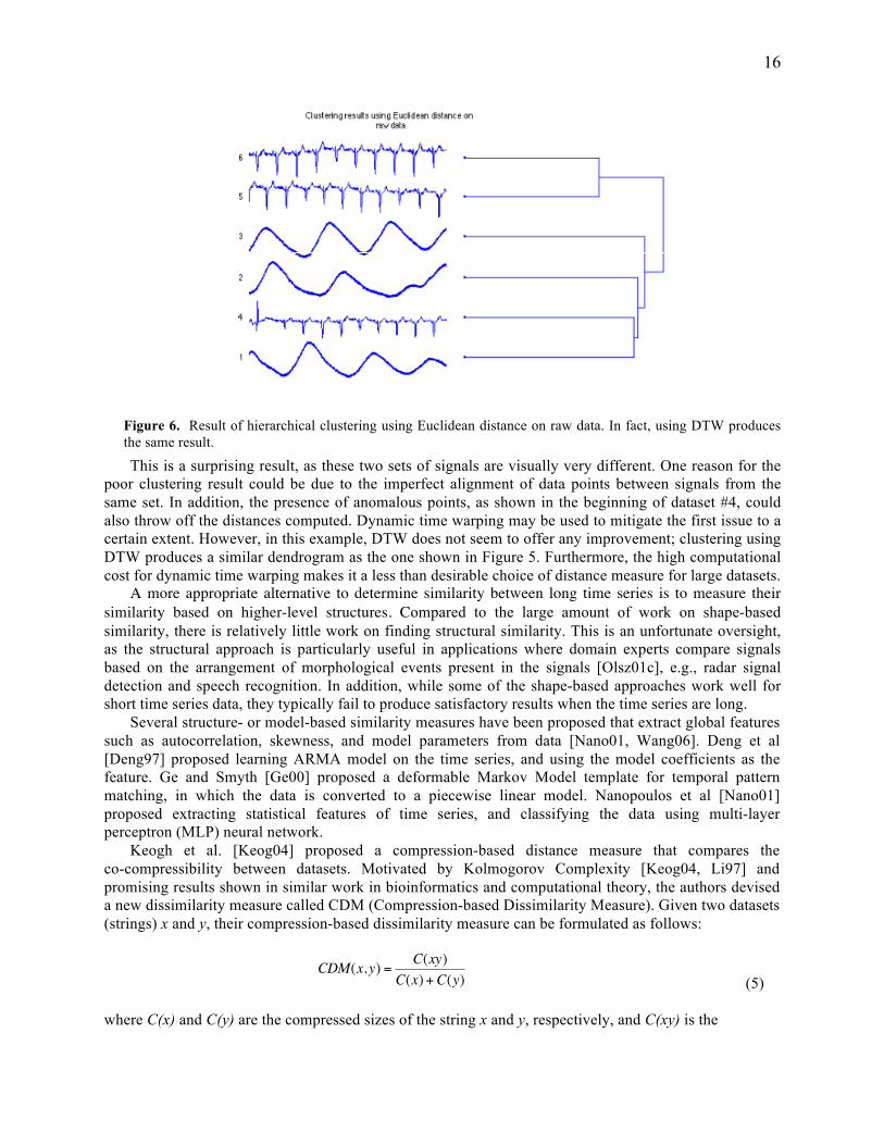
Shape-based similarities work well for short signals or subsequences; however, for long time series data (generally speaking, with a length of hundreds or more), they produce poor results. To illustrate this, we extracted subsequences of length 2048 from six different records on PhysioNet [Goldberger97], an online medical archive containing digital recordings of physiological signals. Signals #1~3 are measurements on respiratory rates, and signals #4~6 are ECG signals. Visually, these two vital signs readouts are readily distinguishable (Figure 6), however, if we try to cluster them using Euclidean distance as the distance measure, the result is disappointing. Figure 6 shows the hierarchical clustering results using Euclidean distance. The dendrogram illustrates that the only datasets that are correctly clustered are datasets #5 and #6 (i.e. they share a common parent node).

16

Figure 6. Result of hierarchical clustering using Euclidean distance on raw data. In fact, using DTW produces the same result.

This is a surprising result, as these two sets of signals are visually very different. One reason for the poor clustering result could be due to the imperfect alignment of data points between signals from the same set. In addition, the presence of anomalous points, as shown in the beginning of dataset #4, could also throw off the distances computed. Dynamic time warping may be used to mitigate the first issue to a certain extent. However, in this example, DTW does not seem to offer any improvement; clustering using DTW produces a similar dendrogram as the one shown in Figure 5. Furthermore, the high computational cost for dynamic time warping makes it a less than desirable choice of distance measure for large datasets.

A more appropriate alternative to determine similarity between long time series is to measure their similarity based on higher-level structures. Compared to the large amount of work on shape-based similarity, there is relatively little work on finding structural similarity. This is an unfortunate oversight, as the structural approach is particularly useful in applications where domain experts compare signals based on the arrangement of morphological events present in the signals [Olsz01c], e.g., radar signal detection and speech recognition. In addition, while some of the shape-based approaches work well for short time series data, they typically fail to produce satisfactory results when the time series are long.

Several structure- or model-based similarity measures have been proposed that extract global features such as autocorrelation, skewness, and model parameters from data [Nano01, Wang06]. Deng et al [Deng97] proposed learning ARMA model on the time series, and using the model coefficients as the feature. Ge and Smyth [Ge00] proposed a deformable Markov Model template for temporal pattern matching, in which the data is converted to a piecewise linear model. Nanopoulos et al [Nano01] proposed extracting statistical features of time series, and classifying the data using multi-layer perceptron (MLP) neural network.

Keogh et al. [Keog04] proposed a compression-based distance measure that compares the co-compressibility between datasets. Motivated by Kolmogorov Complexity [Keog04, Li97] and promising results shown in similar work in bioinformatics and computational theory, the authors devised a new dissimilarity measure called CDM (Compression-based Dissimilarity Measure). Given two datasets (strings) x and y, their compression-based dissimilarity measure can be formulated as follows:

(5)

where C(x) and C(y) are the compressed sizes of the string x and y, respectively, and C(xy) is the

€

CDM(x,y) =C(xy)

C(x)+C(y)

17

compressed size of the concatenated string x+y. The compression-based distance measure is shown to produce superior results compared to other existing structural similarity approaches [Keog04]. Bag-of-Patterns Representation (BOP)

In a previous work, we proposed a histogram-based representation that allows computation of similarity between data based on high-level structure, using a representation similar to the one widely used for text data [Lin09]. In the Vector Space Model [Salt75], a document is represented as a vector: each dimension of the vector corresponds to one word in the vocabulary, and its value is the (relative) frequency of occurrences for the corresponding word in the document. As a result, a p-by-q term-document matrix X is constructed, where p is the number of unique terms in the corpus, q is the number of documents, and each element Xi,j is the frequency of the ith word occurring in the jth document. This “bag of words” representation works well for documents. It is able to capture the structure of a document, without knowing the exact locations or ordering of the words within.

We proposed to represent time series data in a similar fashion, i.e., as a combination of patterns. However, there are two challenges for representing real-valued time series as a “bag of patterns”: (1) how to define patterns, and (2) how to find these patterns. Since time series are composed of real-valued data points, unlike textual data, there are no clear “delimiters” between patterns. In our work, we used a simple sliding-window scheme and the SAX representation to overcome these two challenges.

The algorithm works as follows. First, we construct the pattern “vocabulary” for our time series database. The easiest way to achieve this is to extract subsequences of a fixed length n, normalize the subsequences so they have a mean of zero and standard deviation of one, and then convert them to SAX strings. As a result, we obtain a set of strings, each of which corresponds to a subsequence in the time series. (Recall that SAX has two parameters, α and w.) If we choose α = 4 and w = 8, the resulting dictionary size is αw = 48 = 65,536. Despite its apparent size, the matrix is likely to be sparse, as with textual data. In our experiments, we find that only about 10% of all strings have some subsequence mapped to them [Lin09]. Therefore, we can eliminate words that never occur in any data, or store only the list of occurring SAX strings for each time series.

The construction of the bag-of-patterns matrix is straightforward. The matrix M is a SAX-sequence matrix, analogous to term-document matrices used for information retrieval and text mining. Each row i denotes a SAX string (that is, a pattern) from the pattern vocabulary; each column j denotes a time series; and each Mi,j stores the frequency of string i occurring in time series j. The matrix is a histogram of all pattern counts, which provides a summary for the time series dataset. Once we build the matrix M, we can then use any applicable distance measures, typically Euclidean distance, or dimensionality reduction techniques to compute the similarity between them.

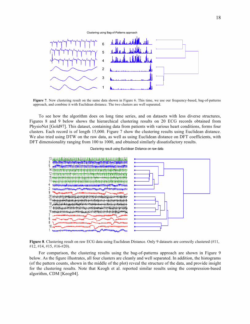
In Figure 6, we showed a simple example where both Euclidean Distance and Dynamic Time Warping on the raw data fail to find the correct clusters. Figure 7 shows the clustering results on the same datasets, using the bag-of-patterns approach. Note we are now clustering on the transformed time series, or the “histogram” of the patterns. For clarity, the original, corresponding time series are also plotted on the left of the dendrogram. We can see clearly that the time series clustered together have similar pattern distribution, which explains why certain datasets are grouped together.

18

Figure 7. New clustering result on the same data shown in Figure 6. This time, we use our frequency-based, bag-of-patterns approach, and combine it with Euclidean distance. The two clusters are well separated.

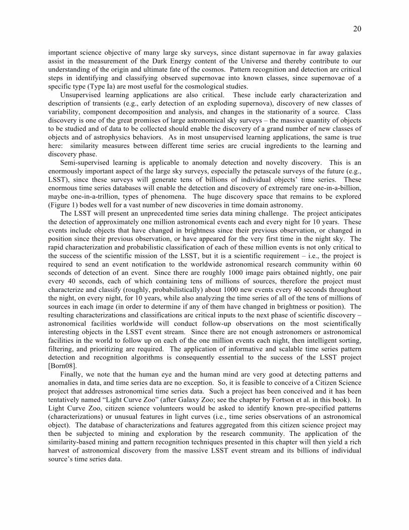
To see how the algorithm does on long time series, and on datasets with less diverse structures,

Figures 8 and 9 below shows the hierarchical clustering results on 20 ECG records obtained from PhysioNet [Gold97]. This dataset, containing data from patients with various heart conditions, forms four clusters. Each record is of length 15,000. Figure 7 show the clustering results using Euclidean distance. We also tried using DTW on the raw data, as well as using Euclidean distance on DFT coefficients, with DFT dimensionality ranging from 100 to 1000, and obtained similarly dissatisfactory results.

Figure 8. Clustering result on raw ECG data using Euclidean Distance. Only 9 datasets are correctly clustered (#11, #12, #14, #15, #16-#20).

For comparison, the clustering results using the bag-of-patterns approach are shown in Figure 9 below. As the figure illustrates, all four clusters are cleanly and well separated. In addition, the histograms (of the pattern counts, shown in the middle of the plot) reveal the structure of the data, and provide insight for the clustering results. Note that Keogh et al. reported similar results using the compression-based algorithm, CDM [Keog04].

19

Figure 9. Clustering result on the same ECG datasets, using our bag-of-patterns approach. All data are clustered correctly. This figure is best viewed in color.

To demonstrate the effectiveness on 1-nearest-neighbor classification, we extracted 250 records from the PhysioNet archive [Gold97]. Each record contains 2048 points. These records are extracted from various databases containing different vital signs, or patients with different heart conditions. We separated the records into 5 classes, and labeled them according to the databases that they are extracted from. We use the leave-one-out cross validation, and count the number of misclassified objects, mc. The error rate is the ratio of mc and the total number of objects (i.e. 250). For this experiment, we also compared with Dynamic Time Warping. The improvement is astounding. The error rate of 0.004 means that there is only 1 misclassified object, out of 250 objects.

Table 6. Classification error rates on three different methods. Our method shows a drastic improvement.

Raw data + Euclidean distance

Raw data + DTW

Bag of Patterns representation + Euclidean distance

Error rate 0.56 0.272 0.004

The results shown above demonstrate that the structure-based similarity measure has the potential of distinguishing different datasets, even when the differences in structures are subtle. Unlike a distance measure that computes point-to-point distances, it captures the global structure of the data consisting of an unordered set of local features, rather than just local differences. This time-invariant feature is useful if we are interested in the overall structures of the time series. At the same time, some orderings are preserved within subsequences. 3. Astronomical Applications: Current and Future As described in Section 1, astronomical time series mining includes supervised, unsupervised, and semi-supervised learning applications (see Bloom & Richards chapter in this book). Classification of stars and other phenomena into one of the known types of variability (described in Section 1) is a very common and traditional astronomy application [Bloo08]. Usually the first step is to determine the type of variability (e.g., periodic, transient, stochastic) and then to determine the specific astrophysical class of object within that variability type. For example, classification of supernovae of different types is a very

20

important science objective of many large sky surveys, since distant supernovae in far away galaxies assist in the measurement of the Dark Energy content of the Universe and thereby contribute to our understanding of the origin and ultimate fate of the cosmos. Pattern recognition and detection are critical steps in identifying and classifying observed supernovae into known classes, since supernovae of a specific type (Type Ia) are most useful for the cosmological studies.

Unsupervised learning applications are also critical. These include early characterization and description of transients (e.g., early detection of an exploding supernova), discovery of new classes of variability, component decomposition and analysis, and changes in the stationarity of a source. Class discovery is one of the great promises of large astronomical sky surveys – the massive quantity of objects to be studied and of data to be collected should enable the discovery of a grand number of new classes of objects and of astrophysics behaviors. As in most unsupervised learning applications, the same is true here: similarity measures between different time series are crucial ingredients to the learning and discovery phase.

Semi-supervised learning is applicable to anomaly detection and novelty discovery. This is an enormously important aspect of the large sky surveys, especially the petascale surveys of the future (e.g., LSST), since these surveys will generate tens of billions of individual objects’ time series. These enormous time series databases will enable the detection and discovery of extremely rare one-in-a-billion, maybe one-in-a-trillion, types of phenomena. The huge discovery space that remains to be explored (Figure 1) bodes well for a vast number of new discoveries in time domain astronomy.

The LSST will present an unprecedented time series data mining challenge. The project anticipates the detection of approximately one million astronomical events each and every night for 10 years. These events include objects that have changed in brightness since their previous observation, or changed in position since their previous observation, or have appeared for the very first time in the night sky. The rapid characterization and probabilistic classification of each of these million events is not only critical to the success of the scientific mission of the LSST, but it is a scientific requirement – i.e., the project is required to send an event notification to the worldwide astronomical research community within 60 seconds of detection of an event. Since there are roughly 1000 image pairs obtained nightly, one pair every 40 seconds, each of which containing tens of millions of sources, therefore the project must characterize and classify (roughly, probabilistically) about 1000 new events every 40 seconds throughout the night, on every night, for 10 years, while also analyzing the time series of all of the tens of millions of sources in each image (in order to determine if any of them have changed in brightness or position). The resulting characterizations and classifications are critical inputs to the next phase of scientific discovery – astronomical facilities worldwide will conduct follow-up observations on the most scientifically interesting objects in the LSST event stream. Since there are not enough astronomers or astronomical facilities in the world to follow up on each of the one million events each night, then intelligent sorting, filtering, and prioritizing are required. The application of informative and scalable time series pattern detection and recognition algorithms is consequently essential to the success of the LSST project [Born08].

Finally, we note that the human eye and the human mind are very good at detecting patterns and anomalies in data, and time series data are no exception. So, it is feasible to conceive of a Citizen Science project that addresses astronomical time series data. Such a project has been conceived and it has been tentatively named “Light Curve Zoo” (after Galaxy Zoo; see the chapter by Fortson et al. in this book). In Light Curve Zoo, citizen science volunteers would be asked to identify known pre-specified patterns (characterizations) or unusual features in light curves (i.e., time series observations of an astronomical object). The database of characterizations and features aggregated from this citizen science project may then be subjected to mining and exploration by the research community. The application of the similarity-based mining and pattern recognition techniques presented in this chapter will then yield a rich harvest of astronomical discovery from the massive LSST event stream and its billions of individual source’s time series data.

21

4 Summary In this chapter, we discuss different approaches for time series pattern recognition. Approaches to pattern recognition tasks vary by representation for the input data, similarity/distance measurement function, and pattern recognition technique. We discuss the various pattern recognition techniques, representations, and similarity measures commonly used for time series. While most existing time series representations proposed in literature are real-valued, in the recent years, the discretization of time series, in particular, using SAX, has become a common practice. Many SAX-based algorithms have been proposed. We discuss two different types of similarity measures: shape-based and structure-based similarity. While the majority of work concentrated on univariate time series, we perform an experimental study on using different similarity measures to classify multivariate time series. We conclude that for classifying short time series, simple techniques, e.g. k-NN as classifier, Euclidean distance as distance measure, and SAX as representation, are just as good as the other more complex approaches, and their efficiency and simplicity offer added advantages. For classifying long time series, a structure-based similarity measure such as CDM or BOP should be considered. We discuss the applicability of time series pattern recognition techniques on astronomy data, as well as the current and future directions for data mining in astronomy.

References [Agra93] Rakesh Agrawal, Christos Faloutsos, and Arun N. Swami (1993). Efficient Similarity Search In Sequence Databases. In Proceedings of the 4th International Conference on Foundations of Data Organization and Algorithms (FODO '93), David B. Lomet (Ed.). Springer-Verlag, London, UK, 69-84 [Agra95] R. Agrawal, G. Psaila, E. L. Wimmers, and M. Zait. Querying Shapes of Histories. In proceedings of the 21st Int'l Conference on Very Large Databases. Zurich, Switzerland. Sept 11-15, 1995. pp. 502-514 [Aitk03] M. J. Aitkenhead, A. J. S. McDonald, A neural network face recognition system, Engineering Applications of Artificial Intelligence, Volume 16, Issue 3, April 2003, Pages 167-176. [Alco01] Alcock, C. et al. (2001). The MACHO Project: Microlensing Detection Efficiency. ApJS 136-439. [Amin06] Morteza Amini, Rasool Jalili, Hamid Reza Shahriari, RT-UNNID: A practical solution to real-time network-based intrusion detection using unsupervised neural networks, Computers & Security, Volume 25, Issue 6, September 2006, Pages 459-468. [Baka05] P. Bakalov, M. Hadjieleftherious, and V. J. Tsotras. Time Relaxed Spatiotemporal Trajectory. In proceedings of the ACM International Symposium on Advances in Geographic Information Systems. Bremen, Germany. Nov 4-5, 2005. [Beye99] Kevin S. Beyer, Jonathan Goldstein, Raghu Ramakrishnan, and Uri Shaft. 1999. When Is ''Nearest Neighbor'' Meaningful?. In Proceedings of the 7th International Conference on Database Theory(ICDT '99), Catriel Beeri and Peter Buneman (Eds.). Springer-Verlag, London, UK, 217-235. [Bloo08] Bloom, J. S., et al. Towards a Real-time Transient Classification Engine. Astronomische Nachrichten, 329, 284, 2008.

22

[Born08] Borne, K. D., A Machine Learning Classification Broker for the LSST Transient Database. Astronomische Nachrichten, 329, 255, 2008. [Bram08] Bramich, D. M., et al. Light and motion in SDSS Stripe 82: the catalogues. Monthly Notices of the Royal Astronomical Society, 386, 887-902, 2008. [Brad98] Bradley, P., Fayyad, U., & Reina, C. (1998). Scaling Clustering Algorithms to Large Databases. In proceedings of the 4th Int'l Conference on Knowledge Discovery and Data Mining. New York, NY, Aug 27-31. pp 9-15. [Came10] Alessandro Camerra, Themis Palpanas, Jin Shieh, Eamonn Keogh, "iSAX 2.0: Indexing and Mining One Billion Time Series," icdm, pp.58-67, 2010 IEEE International Conference on Data Mining, 2010 [Cast10] Nuno Castro, Paulo J. Azevedo: Multiresolution Motif Discovery in Time Series. SDM 2010: 665-676 [Chan99] K. Chan and A. W. Fu. Efficient Time Series Matching by Wavelets. In proceedings of the 15th IEEE Int'l Conference on Data Engineering. Sydney, Australia. Mar 23-26, 1999. pp. 126-133 [Chan09] V. Chandola, D. Cheboli, and V. Kumar, Detecting Anomalies in a Timeseries Database. CS Technical Report 09-004, January 2009, Computer Science Department, University of Minnesota [Chao08] W. A. Chaovalitwongse and P. M. Pardalos. 2008. On the time series support vector machine using dynamic time warping kernel for brain activity classification. Cybernetics and Sys. Anal. 44, 1 (January 2008), 125-138. [Chen04] L. Chen, R. Ng. 2004. On the marriage of Lp-norms and edit distance. In Proceedings of the Thirtieth international conference on Very large data bases - Volume 30 (VLDB '04), 792-803. [Chen05] L. Chen. Similarity Search Over Time Series and Trajectory Data. Ph.D. Dissertation. 2005. University of Waterloo, Waterloo, Ont., Canada, Canada. AAINR03008. [Chen05b] J. S. Chen, Y. S. Moon, and H. W. Yeung. Palmprint Authentication Using Time Series. In proceedings of the 5th International Conference on Audio- and Video-Based Biometric Person Authentication. Hilton Rye Town, NY. July 20-22, 2005. [Chiu03] Chiu, B., Keogh, E., and Lonardi, S. 2003. Probabilistic discovery of time series motifs. InProceedings of the Ninth ACM SIGKDD international Conference on Knowledge Discovery and Data Mining (Washington, D.C., August 24 - 27, 2003). KDD '03. ACM Press, New York, NY, 493-498. [Coll04] Collister, A. A., Lahav, O. ANNz: estimating photometric redshifts using artificial neural networks, astro-ph, 0311058, 2003 [Cort00] C. Cortes, K. Fisher, D. Pregibon, and A. Rogers. Hancock: a language for extracting signatures from data streams. In ACM SIGKDD Intl. Conf. on Knowledge Discoveryand Data Mining, pages 9-17, 2000. [Croc94] M. Crochemore, A. Czumaj, L. Gasjeniec, S. Jarominek, T. Lecroq, W. Plandowski, and W. Rytter. Speeding Up Two String-Matching Algorithms. Algorithmica. vol. 12. pp. 247-267. 1994.

23

[Dasg99] D. Dasgupta and S. Forrest. Novelty Detection in Time Series Data Using Ideas from Immunology. In proceedings of the 8th Int'l Conference on Intelligent Systems. Denver, CO. Jun 24-26, 1999. [Dede10] Gulin Dede, Murat Husnu Sazli, Speech recognition with artificial neural networks, Digital Signal Processing, Volume 20, Issue 3, May 2010, Pages 763-768. [Demp77] Dempster, A., Laird, N., & Rubin, D. (1977). Maximum Likelihood from Incomplete Data via the EM Algorithm. Journal of the Royal Statistical Society, Series B. Vol. 39, No. 1, pp. 1-38. [Deng97] K. Deng, A. Moore, and M. Nechyba, "Learning to Recognize Time Series: Combining ARMA models with Memory-based Learning," IEEE Int. Symp. on Computational Intelligence in Robotics and Automation, Vol. 1, 1997, pp. 246 – 250. [Desa10] Apurva A. Desai, Gujarati handwritten numeral optical character reorganization through neural network, Pattern Recognition, Volume 43, Issue 7, July 2010, Pages 2582-2589. [Ding08] Hui Ding, Goce Trajcevski, Peter Scheuermann, Xiaoyue Wang, and Eamonn Keogh. 2008. Querying and mining of time series data: experimental comparison of representations and distance measures. Proc. VLDB Endow. 1, 2 (August 2008), 1542-1552. [Duda00] Richard O. Duda, Peter E. Hart, and David G. Stork. 2000. Pattern Classification (2nd Edition). Wiley-Interscience. [Eads02] D. Eads, D. Hill, S. Davis, S. Perkins, J. Ma, R. Porter, and J. Theiler. "Genetic Algorithms and Support Vector Machines for Time Series Classification." Proc. SPIE 4787. pp. 74-85. July, 2002 [Falo94] C. Faloutsos, M. Ranganathan, and Y. Manolopulos. Fast Subsequence Matching in Time-Series Databases. SIGMOD Record. vol. 23. pp. 419-429. 1994. [Garg08] Garg, A. (2008). Microlensing candidate selection and detection efficiency for the SuperMACHO Dark Matter search. PhD Thesis. Harvard University. [Ge00] Ge, X. & Smyth, P. Deformable Markov model templates for time-series pattern matching. In proceedings of the 6th ACM SIGKDD. Boston, MA, Aug 20-23, 2000. pp 81-90. [Geur01] P. Geurts. Pattern Extraction for Time Series Classification. In proceedings of the 5th European Conference on Principles of Data Mining and Knowledge Discovery. Freiburg, Germany. 2001. pp. 115-127 [Gold97] Goldberger, A.L., Amaral, L., Glass, L, Hausdorff, J.M., Ivanov, P.Ch., Mark, R.G., Mietus, J.E., Moody, G.B., Peng, C.K., Stanley, H.E.. PhysioBank, PhysioToolkit, and PhysioNet: Circulation 101(23):e215-e220. Discovery, 1(3), 1997. [Han00] Jiawei Han and Micheline Kamber. 2000. Data Mining: Concepts and Techniques. Morgan Kaufmann Publishers Inc., San Francisco, CA, USA. [Hugu06] B. Hugueney. Adaptive Segmentation-Based Symbolic Representation of Time Series for Better Modeling and Lower Bounding Distance Measures. In proceedings of the 10th European Conference on Principles and Practice of Knowledge Discovery in Databases. Berlin, Germany. Sept 18-22, 2006. pp. 545-552

24

[Kado02] M. Kadous. Australian Sign Language Signs (High Quality) Data Set. The UCI KDD Archive, 26 February 2002. http://archive.ics.uci.edu/ml/databases/auslan2/ [Kais04] Kaiser, N. Pan-STARRS: A wide-field optical survey telescope array. Proceedings of the SPIE, 5489, 11-22, 2004. [Kamp09] Argyro Kampouraki, George Manis, and Christophoros Nikou. 2009. Heartbeat time series classification with support vector machines. Trans. Info. Tech. Biomed. 13, 4 (July 2009), 512-518. [Kalp01] K. Kalpakis, D. Gada, and V. Puttagunta. Distance Measures for Effective Clustering of ARIMA Time-Series. In proceedings of the 2001 IEEE In'l Conference on Data Mining. San Jose, CA. Nov 29-Dec 2, 2001. pp. 273-280 [Keog98] E. Keogh and M. Pazzani. An Enhanced Representation of Time Series Which Allows Fast and Accurate Classification, Clustering and Relevance Feedback. In proceedings of the 4th In'l Conference on Knowledge Discovery and Data Mining. New York, NY. Aug 27-31, 1998. pp. 239-241 [Keog04] Keogh, E., Lin, J. & Truppel, W. (2004). Clustering of Time Series Subsequences is Meaningless: Implications for Past and Future Research. Knowledge and Information Systems (KAIS), Springer-Verlag. [Keog01] E. Keogh, K. Chakrabarti, and M. Pazzani. Locally Adaptive Dimensionality Reduction for Indexing Large Time Series Databases. In proceedings of ACM SIGMOD Conference on Management of Data. Santa Barbara. May 21-24, 2001. pp. 151-162 [Keog02] Keogh, E. & Kasetty, S. (2002). On the Need for Time Series Data Mining Benchmarks: A Survey and Empirical Demonstration. In proceedings of the 8th ACM SIGKDD International Conference on Knowledge Discovery. Edmonton, Alberta, Canada. pp 102-111. [Keog02b] E. Keogh. Exact Indexing of Dynamic Time Warping. In Proceedings of the 28th international Conference on Very Large Data Bases. Hong Kong, China, August 20 - 23, 2002. [Keog02c] E. Keogh, S. Lonardi, and B. Chiu. Finding Surprising Patterns in a Time Series Database in Linear Time and Space. In proceedings of the 8th ACM SIGKDD Int'l Conference on Knowledge Discovery and Data Mining. Edmonton, Alberta, Canada. Jul 23-26, 2002. pp. 550-556 [Keog04] Keogh, E., Lonardi, S., and Ratanamahatana, C. A. 2004. Towards parameter-free data mining. In Proceedings of the Tenth ACM SIGKDD international Conference on Knowledge Discovery and Data Mining (Seattle, WA, USA, August 22 - 25, 2004). KDD '04. [Keog04b] Keogh, E. Tutorial in SIGKDD 2004. Data Mining and Machine Learning in Time Series Databases [Keog05] E. Keogh, J. Lin, and A. W. Fu. HOT SAX: Efficiently Finding the Most Unusual Time Series Subsequence. In proceedings of the 5th IEEE International Conference on Data Mining. Houston, TX. Nov 27-30, 2005. pp. 226-233 [Keog06a] Keogh, E., Xi, X., Wei, L. & Ratanamahatana, C. A. (2006). The UCR Time Series Classification/Clustering Homepage: www.cs.ucr.edu/~eamonn/time_series_data/

25

[Keogh06b] Keogh, E., Lin, J. & Fu, A. (2006). Finding the Most Unusual Time Series Subsequence: Algorithms and Applications. Knowledge and Information Systems (KAIS). Springer-Verlag. [Kim07] Kyung-Joong Kim, Sung-Bae Cho, Evolutionary ensemble of diverse artificial neural networks using speciation, Neurocomputing, Volume 71, Issues 7-9, Progress in Modeling, Theory, and Application of Computational Intelligenc - 15th European Symposium on Artificial Neural Networks 2007, 15th European Symposium on Artificial Neural Networks 2007, March 2008, Pages 1604-1618. [Kras07] Vladimir M. Krasnopolsky, Reducing uncertainties in neural network Jacobians and improving accuracy of neural network emulations with NN ensemble approaches, Neural Networks, Volume 20, Issue 4, Computational Intelligence in Earth and Environmental Sciences, May 2007, Pages 454-461. [Lawr90] Lawrence, C. & Reilly, A. (1990). An Expectation Maximization (EM) Algorithm for the Identification and Characterization of Common Sites in Unaligned Biopolymer Sequences. Proteins, Vol. 7, pp 41-51. [Li97] Li, M. & Vitanyi, P. An Introduction to Kolmogorov Complexity and Its Applications. Second Edition, Springer Verlag, 1997. [Liao05] T. Warren Liao. 2005. Clustering of time series data-a survey. Pattern Recogn. 38, 11 (November 2005), 1857 1874. [Lin02] J. Lin, E. Keogh, P. Patel, and S. Lonardi, Finding Motifs in Time Series, the 2nd Workshop on Temporal Data Mining, the 8th ACM Int'l Conference on Knowledge Discovery and Data Mining. Edmonton, Alberta, Canada, 2002, pp. 53-68. [Lin04] Lin, J., Vlachos, M., Keogh, E., & Gunopulos, D. (2004). Iterative Incremental Clustering of Time Series. IX Conference on Extending Database Technology (EDBT). March 14-18, 2004. [Lin07] Jessica Lin, Eamonn J. Keogh, Li Wei, Stefano Lonardi: Experiencing SAX: a novel symbolic representation of time series. Data Min. Knowl. Discov. 15(2): 107-144 (2007) [Lin09] Lin J, Li Y. Finding structural similarity in time series using bag-of-patterns representation. In proceedings of the 21st International Congress on Scientific and Statistical Database Management. New Orleans, LA, June 2-4, 2009 [Lipp87] Lippmann, R.; , "An introduction to computing with neural nets," ASSP Magazine, IEEE , vol.4, no.2, pp. 4- 22, Apr 1987. [Lkha06] B. Lkhagva, Y. Suzuki, and K. Kawagoe. New Time Series Data Representation ESAX for Financial Applications. In proceedings of the 22nd International Conference on Data Engineering Workshops. Atlanta, GA. Apr 3-8, 2006. pp. 115 [Lsst09] LSST Science Collaborations and LSST Project, LSST Science Book, version 2.0, arXiv:0912.0201, http://www.lsst.org/lsst/scibook, 2009 [Mart09] P. Marteau. Time Warp Edit Distance with Stiffness Adjustment for Time Series Matching. IEEE Transactions on Pattern Analysis and Machine Intelligence 31, 2 (February 2009), 306-318. [McGo10] Amy McGovern, Derek H. Rosendahl, Rodger A. Brown, and Kelvin K. Droegemeier, Identifying Predictive Multi-Dimensional Time Series Motifs: An application to severe weather

26

prediction. To appear in Data Mining and Knowledge Discovery, 2010. [McQu67] McQueen, J. (1967). Some Methods for Classification and Analysis of Multivariate Observation. L. Le Cam and J. Neyman (Eds.), In proceedings of the 5th Berkeley Symposium on Mathematical Statistics and Probability, Berkeley, CA. Vol. 1, pp 281-297. [Mink08] Fernanda L. Minku, Teresa B. Ludermir, Clustering and co-evolution to construct neural network ensembles: An experimental study, Neural Networks, Volume 21, Issue 9, November 2008. [Minn06] D. Minnen, T. Starner, I. Essa, C. Isbell. Activity Discovery: Sparse Motifs from Multivariate Time Series. Snowbird Learning Workshop, Snowbird, Utah, April 4-7, 2006. [Minn07] D. Minnen, C.L. Isbell, I. Essa, and T. Starner. Discovering Multivariate Motifs using Subsequence Density Estimation and Greedy Mixture Learning. Twenty-Second Conf. on Artificial Intelligence (AAAI-07), Vancouver, B.C., July 22-26, 2007. [Morc05] F. Morchen and A. Ultsch. Optimizing Time Series Discretization for Knowledge Discovery. In proceedings of the 11th ACM SIGKDD International Conference on Knowledge Discovery and Data Mining. Chicago, IL. Aug 21-24, 2005. pp. 660-665 [Muee09] A. Mueen, E. Keogh, Q. Zhu, S. Cash, and B. Westover. Exact Discovery of Time Series Motifs. In proceedings of the 2009 SIAM International Conference on Data Mining (SDM09). April 30-May 2, 2009. Sparks, NV. [Muee10] Abdullah Mueen and Eamonn Keogh. 2010. Online discovery and maintenance of time series motifs. In Proceedings of the 16th ACM SIGKDD international conference on Knowledge discovery and data mining (KDD '10) [Mura04] K. Murakami, Y. Yano, S. Doki, and S. Okuma. Behavior Extraction from a Series of Observed Robot Motion. In proceedings of JSME Conference on Robotics and Mechatronics. Nagoya, Japan. June, 2004. [Nano01] Nanopoulos, A., Alcock, R., and Manolopoulos, Y. 2001. Feature-based classification of time-series data. In information Processing and Technology, N. Mastorakis and S. D. Nikolopoulos, Eds. Nova Science Publishers, Commack, NY, 49-61. [Olsz01c] R. Olszewski. Generalized Feature Extraction for Structural Pattern Recognition in Time-Series Data. PhD thesis, Carnegie Mellon University, Pittsburgh, PA, 2001. [Pres09] Dan Preston, Pavlos Protopapas, Carla Brodley. Event Discovery in Time Series. SDM 2009. [Pome89] D.A. Pomerleau, “ALVINN: An Autonomous Land Vehicle in a Neural Network,” Technical Report CMU-CS-89-107, Carnegie Mellon Univ., 1989. [Poug06] F. Pouget, G. Urvoy-Keller, and M. Dacier. Time Signature to Detect Multi-Headed Stealthy Attack Tools. In proceedings of the 18th Annual FIRST Conference. Baltimore, MD. June 25-30, 2006 [Rado10] Milos Radovanovic, Alexandros Nanopoulos, Mirjana Ivanovic: Time-Series Classification in Many Intrinsic Dimensions. SDM 2010: 677-688

27

[Rata04] Ratanamahatana, C. A. and Keogh. E. (2004). Making Time-series Classification More Accurate Using Learned Constraints. In proceedings of SIAM International Conference on Data Mining (SDM '04), Lake Buena Vista, Florida, April 22-24, 2004. pp. 11-22. [Rau09] Rau, A., et al. Exploring the Optical Transient Sky with the Palomar Transient Factory. Publications of the Astronomical Society of the Pacific, 886, 1334-1351, 2009. [Rebb09] Umaa Rebbapragada, Pavlos Protopapas, Carla E. Brodley, Charles R. Alcock: Finding anomalous periodic time series. Machine Learning 74(3): 281-313 (2009) [Rodr05] Juan José Rodríguez, Carlos J. Alonso, José A. Maestro: Support vector machines of interval-based features for time series classification.Knowl.-Based Syst. 18(4-5): 171-178 (2005) [Rodr06] P.P. Rodrigues, J. Gama, and J.P. Pedroso, “ODAC: Hierarchical Clustering of Time Series Data Streams,” Proc. Sixth SIAM Int'l Conf. Data Mining, pp. 499-503, Apr. 2006. [Rose58] Rosenblatt, F. The perceptron: A probabilistic model for information storage and organization in the brain. Psychological Review, Vol 65(6), Nov 1958, 386-408 [Salto75] Salton, G., Wong, A., and Yang, C. S. 1975. A vector space model for automatic indexing. Commun. ACM 19, 11 (Nov. 1975), 613-620. [Shie08] Jin Shieh and Eamonn Keogh. 2008. iSAX: indexing and mining terabyte sized time series. In Proceeding of the 14th ACM SIGKDD international conference on Knowledge discovery and data mining (KDD ’08). ACM, New York, NY, USA, 623-631. [Star08] Starr, D., Bloom, J. and Brewer, J. (2008). Realtime Astronomical Time-series Classification and Broadcast Pipeline. In proceedings of the 7th Python in Science Conference. [Szym05] Szymanski, M. K. The Optical Gravitational Lensing Experiment. Internet Access to the OGLE Photometry Data Set: OGLE-II BVI maps and I-band data. Acta Astronomica 55, 43-57, 2005. [Tang08] H. Tang and S.S. Liao. Discovering original motifs with different lengths from time series. Know.-Based Syst. 21, 7 (Oct. 2008), 666-671. [Vapn98] Vapnik, V. “Estimating the Values of Function at Given Points”, Statistical Learning Theory, Wiley-Interscience, New York, 1998. [Vlac02] Michail Vlachos, Dimitrios Gunopoulos, and George Kollios. 2002. Discovering Similar Multidimensional Trajectories. In Proceedings of the 18th International Conference on Data Engineering (ICDE '02). [Wang06] Wang, X., Smith, K., and Hyndman, R. 2006. Characteristic-Based Clustering for Time Series Data. Data Min. Knowl. Discov. 13, 3 (Nov. 2006), 335-364. [Wang09] Wang, T., Huang, J.-S., & Gu, Q.-S. (2009). Photometric redshifts of galaxies from SDSS and 2MASS. Research in Astronomy and Astrophysics, 9(4), 390-400. [Wei06] Li Wei and Eamonn Keogh. 2006. Semi-supervised time series classification. In Proceedings of the 12th ACM SIGKDD international conference on Knowledge discovery and data mining (KDD '06). ACM, New York, NY, USA, 748-753.

28

[Yi00] B. K. Yi and C. Faloutsos. Fast Time Sequence Indexing for Arbitrary Lp Norms. In proceedings of the 26th Int'l Conference on Very Large Databases. Cairo, Egypt. Sep 10-14, 2000. pp. 385-394 [Zhou02] Zhi-Hua Zhou, Jianxin Wu, Wei Tang, Ensembling neural networks: Many could be better than all, Artificial Intelligence, Volume 137, Issues 1-2, May 2002, Pages 239-263. [Zhu05] Zhu, X. (2005). Semi-supervised learning literature survey. Technical report, no. 1530, Computer Sciences, University of Wisconsin-Madison, 2005.