Data Acquisition and View Planning for 3-D Modeling Tasks

Paul S. Blaer and Peter K. Allen

Abstract— In this paper we address the joint problems ofautomated data acquisition and view planning for large–scaleindoor and outdoor sites. Our method proceeds in two distinctstages. In the initial stage, the system is given a 2-D map withwhich it plans a minimal set of sufficient covering views. Wethen use a 3-D laser scanner to take scans at each of these views.When this planning system is combined with our mobile robot,it automatically computes and executes a tour of these viewinglocations and acquires the views with the robot’s onboard laserscanner. These initial scans serve as an approximate 3-D modelof the site. The planning software then enters a second stage inwhich it updates this model by using a voxel-based occupancyprocedure to plan the next best view. This next best view isacquired, and further next best views are sequentially computedand acquired until a complete 3-D model is obtained. Resultsare shown for Fort Jay on Governors Island in the City of NewYork and for the church of Saint Menoux in the Bourbonnaisregion of France.

I. INTRODUCTION

Dense and detailed 3-D models of large structures canbe useful in many fields. These models can allow engineersto analyze the stability of a structure and then test possiblecorrections without endangering the original. The models canalso provide documentation of historical sites in danger ofdestruction and archaeological sites at various stages of anexcavation. With detailed models, professionals and studentscan tour such sites from thousands of miles away.

Modern laser range scanners will quickly generate a densepoint cloud of measurements; however, many of the stepsneeded for 3-D model construction require time-consuminghuman involvement. These steps include the planning of theviewing locations as well as the acquisition of the data atmultiple viewing locations. By automating these tasks, wewill ultimately be able to speed this process significantly.A plan must be laid out to determine where to take eachindividual scan. This requires choosing efficient views thatwill cover the entire surface area of the structure withoutocclusions from other objects and without self occlusionsfrom the target structure itself. This is the essence of the so–called view planning problem. Manually choosing the viewscan be time consuming in itself. Then the scanning sensormust be physically moved from location to location whichis also time consuming and physically stressful.

Funded by NSF grants IIS-0121239 and ANI-00-99184.Thanks to the National Park Service for granting us access to Governors

Island and to the Governors Island staff: Linda Neal, Ed Lorenzini, MikeShaver, Ilyse Goldman, and Dena Saslaw for their invaluable assistance.

Thanks to the scanning team of Hrvoje Benko, Matei Ciocarlie, AtanasGeorgiev, Corey Goldfeder, Chase Hensel, Tie Hu, and Claire Lackner.

Both authors are with the Department of Computer Science, ColumbiaUniversity, New York, NY 10027, USA

E-mail: {pblaer, allen}@cs.columbia.edu

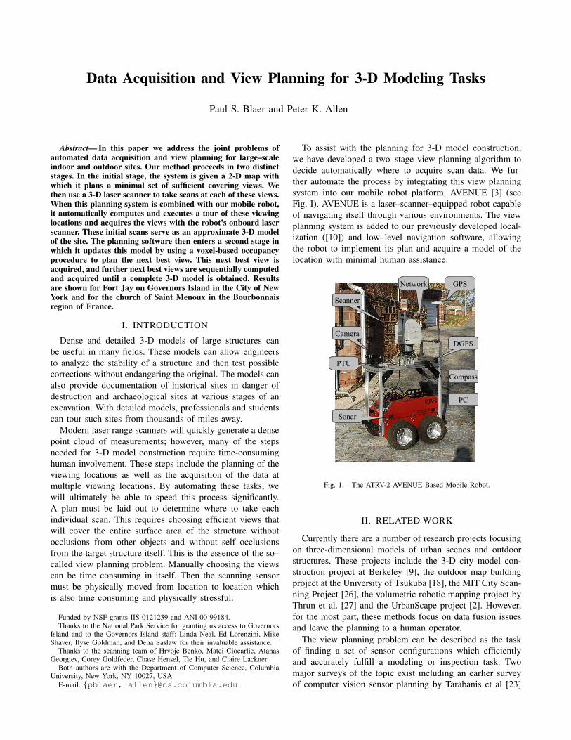
To assist with the planning for 3-D model construction,we have developed a two–stage view planning algorithm todecide automatically where to acquire scan data. We fur-ther automate the process by integrating this view planningsystem into our mobile robot platform, AVENUE [3] (seeFig. I). AVENUE is a laser–scanner–equipped robot capableof navigating itself through various environments. The viewplanning system is added to our previously developed local-ization ([10]) and low–level navigation software, allowingthe robot to implement its plan and acquire a model of thelocation with minimal human assistance.

GPS

DGPS

PC

Compass

Sonar

Network

Scanner

Camera

PTU

Fig. 1. The ATRV-2 AVENUE Based Mobile Robot.

II. RELATED WORK

Currently there are a number of research projects focusingon three-dimensional models of urban scenes and outdoorstructures. These projects include the 3-D city model con-struction project at Berkeley [9], the outdoor map buildingproject at the University of Tsukuba [18], the MIT City Scan-ning Project [26], the volumetric robotic mapping project byThrun et al. [27] and the UrbanScape project [2]. However,for the most part, these methods focus on data fusion issuesand leave the planning to a human operator.

The view planning problem can be described as the taskof finding a set of sensor configurations which efficientlyand accurately fulfill a modeling or inspection task. Twomajor surveys of the topic exist including an earlier surveyof computer vision sensor planning by Tarabanis et al [23]

and a more recent survey of view planning specifically for3-D vision by Scott et al [21].

The model-based methods are the inspection methodsin which the system is given some initial model of thescene. Early research focused on planning for 2-D camera-based systems. Included in this are works by Cowan andKovesi [7] and by Tarabanis et al. [24]. Later, these methodswere extended to the 3-D domain in works by Tarboxand Gottschlich [25]. We can also include the art galleryproblems in this category. In two dimensions, these problemscan be approached with traditional geometric solutions suchas in Xie et al. [28] or with randomized methods such asin Gonzalez-Banos et al. [11]. The art gallery approach hasbeen applied to 3-D problems by Danner and Kavraki [8].

The non-model-based methods seek to generate modelswith no prior information. These include volumetric methodssuch as in Connolly [6], Massios and Fisher [15], and Lowet al. [14]. There are also surface-based methods whichinclude Maver and Bajcsy [16], Pito [19], Reed and Allen[20], and Sequeira et al ([22]). View planning for 2-D mapconstruction with a mobile robot is addressed by Gonzalez-Banos et al [12]. Nuchter et al [17] address view planning for3-D scenes with a mobile robot. Next best views are chosenby maximizing the amount of 2-D information (informationon the ground plane only) that can be obtained at a chosenlocation; however, 3-D data are actually acquired.

III. THE TWO STAGE PLANNING ALGORITHM

A. Phase 1: Initial Model Construction

In the first stage of our modeling process, we wish tocompute and acquire an initial model of the target region.This model will be based on limited information about thesite and will likely have gaps which must be filled in duringthe second stage of the process. The data acquired in theinitial stage will serve as a seed for the boostrapping methodused to complete the model.

The procedure for planning the initial views makes useof a two-dimensional map of the region to plan a series ofenvironment views for our scanning system to acquire. Mapssuch as these are commonly available for large scale sites.All scanning locations in this initial phase are planned inadvance, before any data acquisition occurs.

Planning these locations resembles the art gallery problem,which asks where to optimally place guards such that allwalls of the art gallery can be seen by the guards. We wishto find a set of positions for our scanner such that it canimage all of the walls in our 2-D environment map. Thisview planning strategy makes the assumption that if we cansee the 2-D footprint of a wall then we can see the wall in3-D. In practice, this is rarely the case, because a 3-D partof a wall that is not visible in the 2-D map might obstructanother part of the scene. However, for an initial model ofthe scene to be used later for refinement, this assumptionshould give us sufficient coverage.

The traditional art gallery problem assumes that the guardshave a 360 degree field of view, have an unlimited range,

and can view a wall at any grazing angle. None of these as-sumptions are true for most laser scanners, so the traditionalmethods do not apply to our problem. Gonzalez-Banos etal [11] proposed a randomized method for approximatingsolutions to the art gallery problems. We have chosen toextend their randomized algorithm to include the visibilityconstraints of our sensor.

In our version of the randomized algorithm, a set of initialscanning locations are randomly distributed throughout thefree space of the region to be imaged. The visibility polygonof each of these points is then computed based on theconstraints of our sensor. Finally, an approximation for theoptimal number of viewpoints needed to cover the boundariesof the free space is computed from this set of initial locations.

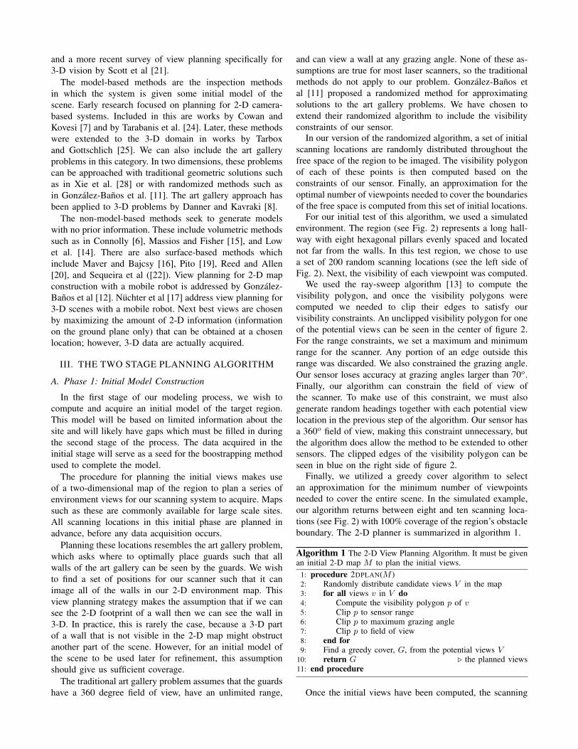
For our initial test of this algorithm, we used a simulatedenvironment. The region (see Fig. 2) represents a long hall-way with eight hexagonal pillars evenly spaced and locatednot far from the walls. In this test region, we chose to usea set of 200 random scanning locations (see the left side ofFig. 2). Next, the visibility of each viewpoint was computed.

We used the ray-sweep algorithm [13] to compute thevisibility polygon, and once the visibility polygons werecomputed we needed to clip their edges to satisfy ourvisibility constraints. An unclipped visibility polygon for oneof the potential views can be seen in the center of figure 2.For the range constraints, we set a maximum and minimumrange for the scanner. Any portion of an edge outside thisrange was discarded. We also constrained the grazing angle.Our sensor loses accuracy at grazing angles larger than 70o.Finally, our algorithm can constrain the field of view ofthe scanner. To make use of this constraint, we must alsogenerate random headings together with each potential viewlocation in the previous step of the algorithm. Our sensor hasa 360o field of view, making this constraint unnecessary, butthe algorithm does allow the method to be extended to othersensors. The clipped edges of the visibility polygon can beseen in blue on the right side of figure 2.

Finally, we utilized a greedy cover algorithm to selectan approximation for the minimum number of viewpointsneeded to cover the entire scene. In the simulated example,our algorithm returns between eight and ten scanning loca-tions (see Fig. 2) with 100% coverage of the region’s obstacleboundary. The 2-D planner is summarized in algorithm 1.

Algorithm 1 The 2-D View Planning Algorithm. It must be givenan initial 2-D map M to plan the initial views.

1: procedure 2DPLAN(M )2: Randomly distribute candidate views V in the map3: for all views v in V do4: Compute the visibility polygon p of v5: Clip p to sensor range6: Clip p to maximum grazing angle7: Clip p to field of view8: end for9: Find a greedy cover, G, from the potential views V

10: return G . the planned views11: end procedure

Once the initial views have been computed, the scanning

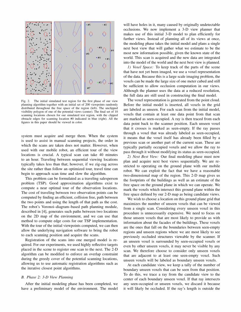
Fig. 2. The initial simulated test region for the first phase of our viewplanning algorithm together with an initial set of 200 viewpoints randomlydistributed throughout the free space of the region (left). The unclippedvisibility polygon of one of the potential views (center). The final set of 10scanning locations chosen for our simulated test region, with the clippedobstacle edges for scanning location #0 indicated in blue (right). All thefigures in this paper should be viewed in color.

system must acquire and merge them. When the systemis used to assist in manual scanning projects, the order inwhich the scans are taken does not matter. However, whenused with our mobile robot, an efficient tour of the viewlocations is crucial. A typical scan can take 40 minutesto an hour. Traveling between sequential viewing locationstypically takes less than that; however, if we zig-zag acrossthe site rather than follow an optimized tour, travel time canbegin to approach scan time and slow the algorithm.

This problem can be formulated as a traveling salespersonproblem (TSP). Good approximation algorithms exist tocompute a near optimal tour of the observation locations.The cost of traveling between two observation points can becomputed by finding an efficient, collision free, path betweenthe two points and using the length of that path as the cost.The robot’s Voronoi–diagram–based path planning module,described in [4], generates such paths between two locationson the 2D map of the environment, and we can use thatmethod to compute edge costs for our TSP implementation.With the tour of the initial viewpoints computed, we can thenallow the underlying navigation software to bring the robotto each scanning position and acquire the scans.

Registration of the scans into one merged model is re-quired. For our experiments, we used highly reflective targetsplaced in the scene to register one scan to the next. The 2-Dalgorithm can be modified to enforce an overlap constraintduring the greedy cover of the potential scanning locations,allowing us to use automatic registration algorithms such asthe iterative closest point algorithms.

B. Phase 2: 3-D View Planning

After the initial modeling phase has been completed, wehave a preliminary model of the environment. The model

will have holes in it, many caused by originally undetectableocclusions. We now implement a 3-D view planner thatmakes use of this initial 3-D model to plan efficiently forfurther views. Instead of planning all of its views at once,the modeling phase takes the initial model and plans a singlenext best view that will gather what we estimate to be themost new information possible, given the known state of theworld. This scan is acquired and the new data are integratedinto the model of the world and the next best view is planned.

1) Voxel Space: To keep track of the parts of the scenethat have not yet been imaged, we use a voxel representationof the data. Because this is a large scale imaging problem, thevoxels can be made the large size of one meter cubed and stillbe sufficient to allow occlusion computation in our views.Although the planner uses the data at a reduced resolution,the full data are still used in constructing the final model.

The voxel representation is generated from the point cloud.Before the initial model is inserted, all voxels in the gridare labeled as unseen. For each scan from the initial model,voxels that contain at least one data point from that scanare marked as seen-occupied. A ray is then traced from eachdata point back to the scanner position. Each unseen voxelthat it crosses is marked as seen-empty. If the ray passesthrough a voxel that was already labeled as seen-occupied,it means that the voxel itself has already been filled by aprevious scan or another part of the current scan. These aretypically partially occupied voxels and we allow the ray topass through it without modifying its status as seen-occupied.

2) Next Best View: Our final modeling phase must nowplan and acquire next best views sequentially. We are re-stricted to operating on the ground plane with our mobilerobot. We can exploit the fact that we have a reasonabletwo-dimensional map of the region. This 2-D map gives usthe footprints of the buildings as well as an estimate of thefree space on the ground plane in which we can operate. Wemark the voxels which intersect this ground plane within thefree space defined by our 2-D map as being candidate views.

We wish to choose a location on this ground plane grid thatmaximizes the number of unseen voxels that can be viewedfrom a single scan. Considering every unseen voxel in thisprocedure is unnecessarily expensive. We need to focus onthose unseen voxels that are most likely to provide us withinformation about the facades of the buildings. These voxelsare the ones that fall on the boundaries between seen-emptyregions and unseen regions where we are most likely to seepreviously occluded structures viewable by the scanner. Ifan unseen voxel is surrounded by seen-occupied voxels oreven by other unseen voxels, it may never be visible by anyscan. We therefore choose to consider only unseen voxelsthat are adjacent to at least one seen-empty voxel. Suchunseen voxels will be labeled as boundary unseen voxels.

At each candidate view, we keep a tally of the number ofboundary unseen voxels that can be seen from that position.To do this, we trace a ray from the candidate view to thecenter of each boundary unseen voxel. If that ray intersectsany seen-occupied or unseen voxels, we discard it becauseit will likely be occluded. If the ray’s length is outside the

scanner’s range, then we discard the ray as well. If a ray hasnot been discarded by either the occlusion or range condition,we can safely increment the tally of the candidate viewfrom which the ray emanates. At the end of this calculation,the ground plane position with the highest tally is chosenas the next scan location. When using the mobile robot, itagain computes the Voronoi-based path and navigates to thechosen position. It triggers a scan once it has arrived, and thatscan is integrated into the point cloud model and the voxelrepresentation. This second stage is repeated until we reach asufficient level of coverage. To terminate the algorithm, welook at the number of boundary unseen voxels that wouldbe resolved by the next iteration. If that number falls belowsome threshold value, the algorithm terminates; otherwise, itcontinues. The 3-D planner is summarized in algorithm 2.

Algorithm 2 The 3-D View Planning Algorithm. It must be givenan initial model of the world C, a set of possible scanning locationsP , and a threshold value for unseen voxels as a stopping condition.

1: procedure 3DPLAN(C,P ,threshold)2: Initialize voxel space from C3: for all unseen voxels, u, in the voxel space do4: if u has a seen empty neighbor then5: add u to U . the set of boundary unseen voxels6: end if7: end for8: loop9: for all potential views p in P do

10: Count members of U that are visible11: end for12: if maxcount(p) < threshold then13: break14: end if15: Acquire scan at p with largest count16: Merge new scan into C and update voxel space17: Recompute U from the new voxel space18: end loop19: return C . the updated model20: end procedure

The algorithm is similar to a brute force computation.If the size of one dimension of the voxel grid is n, therecould be O(n2) potential viewing locations. If there are mboundary unseen voxels, the cost of the algorithm could be ashigh as O(n2∗m). However, this cost is not prohibitive. m issmall in comparison to the total number of voxels and manyof the n2 ground plane voxels are not potential view pointsbecause they fall within known obstacles. Furthermore, sincemost boundary unseen voxels only have one face exposedto the known world, the majority of the potential scanninglocations can be quickly excluded.

IV. EXPERIMENTAL RESULTS

A. Phase 1 Applied Indoors and Outdoors

1) Saint Menoux: As part of a larger 3-D modelingeffort, we have been involved in modeling the Romanesquechurches of the Bourbonnais region of France [1]. We testedour 2-D planning algorithm in several of those churches,including the interior of the church of Saint Menoux. Inthis indoor experiment, we tested the algorithm itself by

Fig. 3. On the left is the 2-D map of Saint Menoux’s interior. Also shownare the 8 scan locations determined by the initial two-dimensional viewplanner using a grazing angle constraint of 70o. On the right is a slicetaken at floor level of the complete model acquired after taking all 8 scans.

moving our 360o field of view scanner manually to eachof the planned views. We could not use the mobile robotindoors here because the robot makes extensive use of GPSin its navigation routines and GPS is typically not usablein an indoor environment. Also, the curch had a particularlycluttered environment containing numerous chairs and tablesthat left paths that were too narrow for our robot. However,as a sensor planning technique, our algorithms were veryuseful, even to human scanners.

For our test, we set the threshold such that the algorithmterminated if additional scans added less than 2% of thetotal boundaries of the target region. Our algorithm returnedeight scanning locations for the test area (see the left ofFig. 3) giving us a coverage of 95% of the region’s obstacleboundary. In figure 3 we show a floor level slice of theresulting interior model of the church. In this experiment,as with all others, scans were merged using reflective targetsscattered throughout the environment for registration.

2) Fort Jay: Fort Jay is a large fort located on GovernorsIsland in the City of New York. With the kind permissionof the National Park Service, we used this as our outdoortest bed for the system. We were given a floor plan of thefort which we divided into three distinct sections: the innercourtyard, the outer courtyard, and the moat.

We split the fort into these three sections because thetransitions between them were not easily traversable by therobot. Also, because of sloped terrain, the robot could notoperate in the outer courtyard or moat. As a result, these twoouter regions were acquired by using our planning algorithmto make the decisions and then placing the scanner manuallyat the scanning locations. For the inner courtyard modeling,the mobile robot chose the scanning locations, planned thetour of those positions, and traversed the path, allowing us

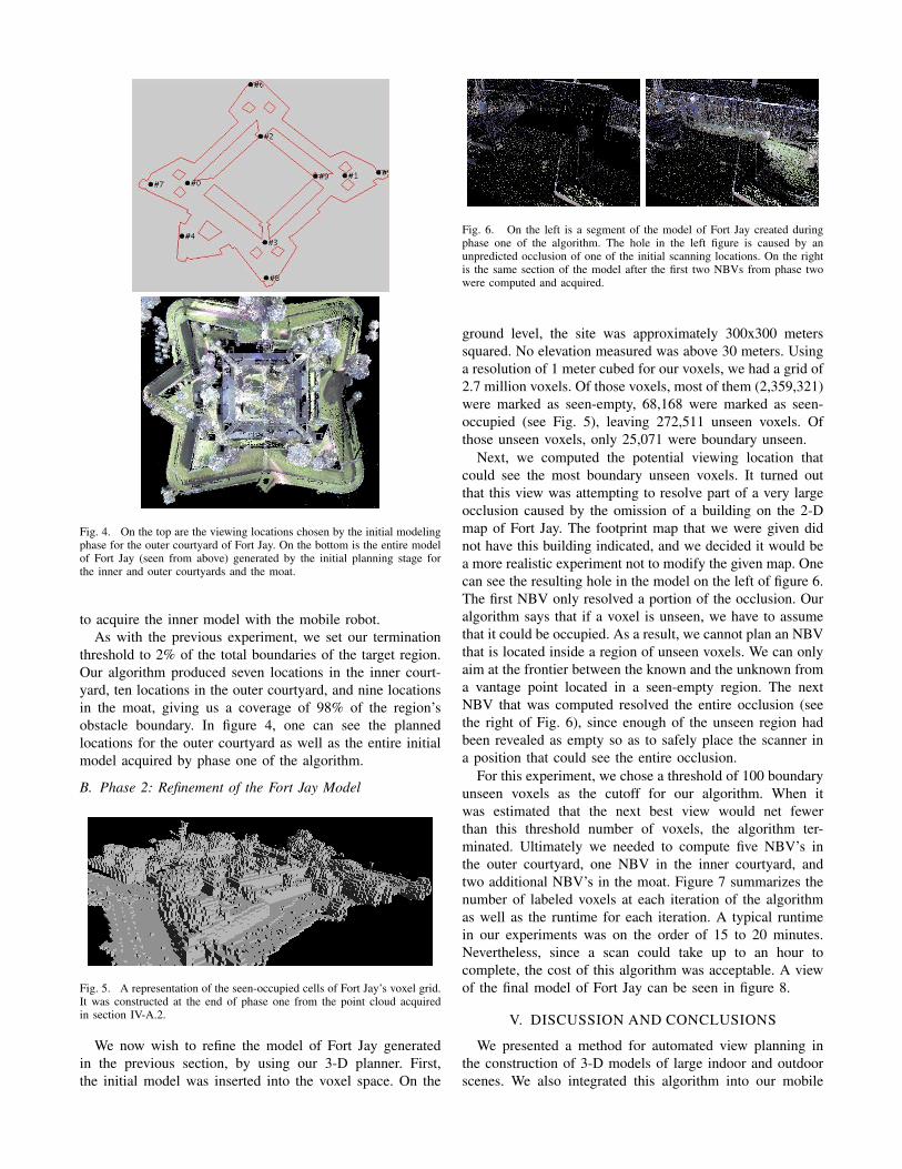
Fig. 4. On the top are the viewing locations chosen by the initial modelingphase for the outer courtyard of Fort Jay. On the bottom is the entire modelof Fort Jay (seen from above) generated by the initial planning stage forthe inner and outer courtyards and the moat.

to acquire the inner model with the mobile robot.As with the previous experiment, we set our termination

threshold to 2% of the total boundaries of the target region.Our algorithm produced seven locations in the inner court-yard, ten locations in the outer courtyard, and nine locationsin the moat, giving us a coverage of 98% of the region’sobstacle boundary. In figure 4, one can see the plannedlocations for the outer courtyard as well as the entire initialmodel acquired by phase one of the algorithm.

B. Phase 2: Refinement of the Fort Jay Model

Fig. 5. A representation of the seen-occupied cells of Fort Jay’s voxel grid.It was constructed at the end of phase one from the point cloud acquiredin section IV-A.2.

We now wish to refine the model of Fort Jay generatedin the previous section, by using our 3-D planner. First,the initial model was inserted into the voxel space. On the

Fig. 6. On the left is a segment of the model of Fort Jay created duringphase one of the algorithm. The hole in the left figure is caused by anunpredicted occlusion of one of the initial scanning locations. On the rightis the same section of the model after the first two NBVs from phase twowere computed and acquired.

ground level, the site was approximately 300x300 meterssquared. No elevation measured was above 30 meters. Usinga resolution of 1 meter cubed for our voxels, we had a grid of2.7 million voxels. Of those voxels, most of them (2,359,321)were marked as seen-empty, 68,168 were marked as seen-occupied (see Fig. 5), leaving 272,511 unseen voxels. Ofthose unseen voxels, only 25,071 were boundary unseen.

Next, we computed the potential viewing location thatcould see the most boundary unseen voxels. It turned outthat this view was attempting to resolve part of a very largeocclusion caused by the omission of a building on the 2-Dmap of Fort Jay. The footprint map that we were given didnot have this building indicated, and we decided it would bea more realistic experiment not to modify the given map. Onecan see the resulting hole in the model on the left of figure 6.The first NBV only resolved a portion of the occlusion. Ouralgorithm says that if a voxel is unseen, we have to assumethat it could be occupied. As a result, we cannot plan an NBVthat is located inside a region of unseen voxels. We can onlyaim at the frontier between the known and the unknown froma vantage point located in a seen-empty region. The nextNBV that was computed resolved the entire occlusion (seethe right of Fig. 6), since enough of the unseen region hadbeen revealed as empty so as to safely place the scanner ina position that could see the entire occlusion.

For this experiment, we chose a threshold of 100 boundaryunseen voxels as the cutoff for our algorithm. When itwas estimated that the next best view would net fewerthan this threshold number of voxels, the algorithm ter-minated. Ultimately we needed to compute five NBV’s inthe outer courtyard, one NBV in the inner courtyard, andtwo additional NBV’s in the moat. Figure 7 summarizes thenumber of labeled voxels at each iteration of the algorithmas well as the runtime for each iteration. A typical runtimein our experiments was on the order of 15 to 20 minutes.Nevertheless, since a scan could take up to an hour tocomplete, the cost of this algorithm was acceptable. A viewof the final model of Fort Jay can be seen in figure 8.

V. DISCUSSION AND CONCLUSIONS

We presented a method for automated view planning inthe construction of 3-D models of large indoor and outdoorscenes. We also integrated this algorithm into our mobile

At the Seen Boundary Visible Runtimeend of: Occupied Unseen to NBV (minutes)

2-D Plan 68,168 25,071 1,532 21.25NBV 1 70,512 21,321 1,071 19.30NBV 2 71,102 18,357 953 18.93NBV 3 72,243 17,156 948 18.72NBV 4 73,547 15,823 812 16.59NBV 5 74,451 14,735 761 16.43NBV 6 75,269 13,981 421 15.82NBV 7 75,821 13,519 255 15.60NBV 8 76,138 13,229 98 15.22

Fig. 7. A summary of the number of labeled voxels after each iteration ofthe 3-D planning algorithm. The next to last column indicates the numberof boundary unseen voxels that are actually visible to the next best view.

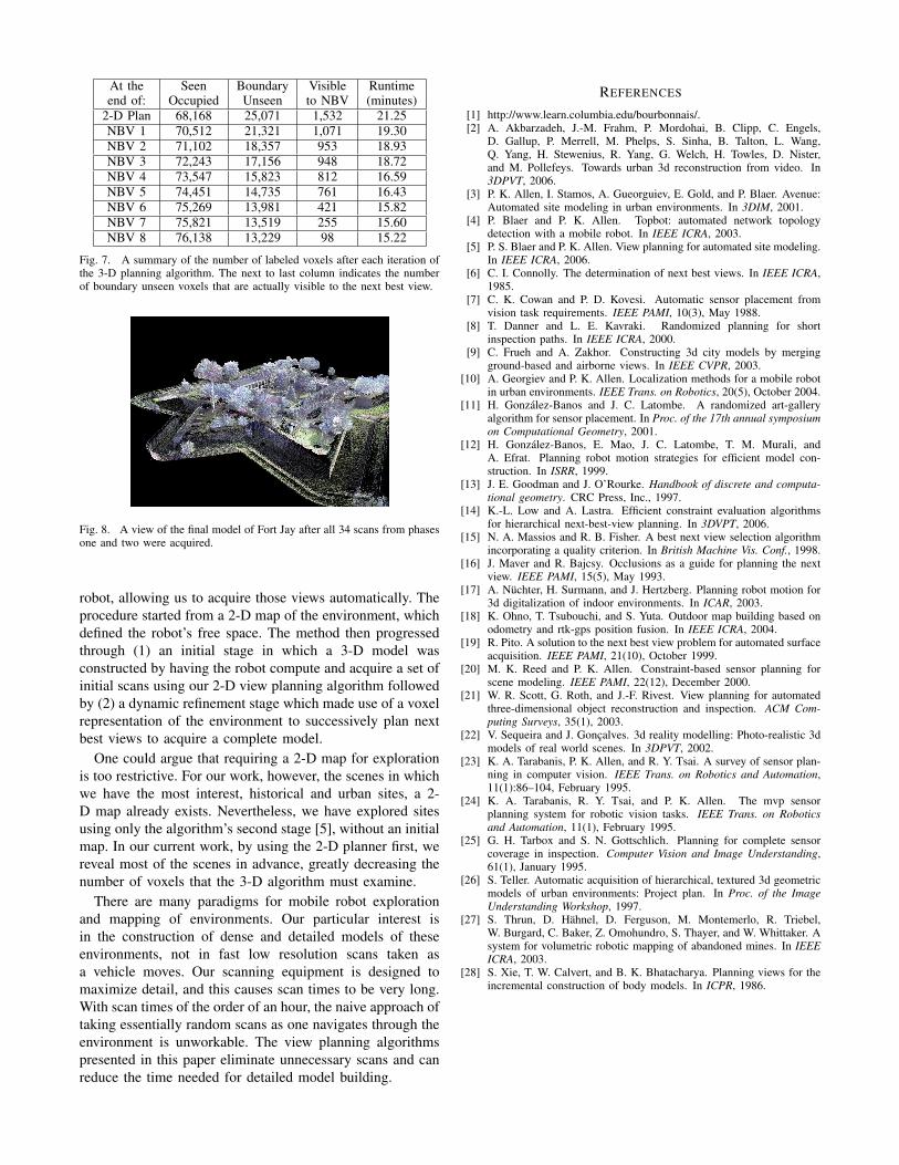
Fig. 8. A view of the final model of Fort Jay after all 34 scans from phasesone and two were acquired.

robot, allowing us to acquire those views automatically. Theprocedure started from a 2-D map of the environment, whichdefined the robot’s free space. The method then progressedthrough (1) an initial stage in which a 3-D model wasconstructed by having the robot compute and acquire a set ofinitial scans using our 2-D view planning algorithm followedby (2) a dynamic refinement stage which made use of a voxelrepresentation of the environment to successively plan nextbest views to acquire a complete model.

One could argue that requiring a 2-D map for explorationis too restrictive. For our work, however, the scenes in whichwe have the most interest, historical and urban sites, a 2-D map already exists. Nevertheless, we have explored sitesusing only the algorithm’s second stage [5], without an initialmap. In our current work, by using the 2-D planner first, wereveal most of the scenes in advance, greatly decreasing thenumber of voxels that the 3-D algorithm must examine.

There are many paradigms for mobile robot explorationand mapping of environments. Our particular interest isin the construction of dense and detailed models of theseenvironments, not in fast low resolution scans taken asa vehicle moves. Our scanning equipment is designed tomaximize detail, and this causes scan times to be very long.With scan times of the order of an hour, the naive approach oftaking essentially random scans as one navigates through theenvironment is unworkable. The view planning algorithmspresented in this paper eliminate unnecessary scans and canreduce the time needed for detailed model building.

REFERENCES

[1] http://www.learn.columbia.edu/bourbonnais/.[2] A. Akbarzadeh, J.-M. Frahm, P. Mordohai, B. Clipp, C. Engels,

D. Gallup, P. Merrell, M. Phelps, S. Sinha, B. Talton, L. Wang,Q. Yang, H. Stewenius, R. Yang, G. Welch, H. Towles, D. Nister,and M. Pollefeys. Towards urban 3d reconstruction from video. In3DPVT, 2006.

[3] P. K. Allen, I. Stamos, A. Gueorguiev, E. Gold, and P. Blaer. Avenue:Automated site modeling in urban environments. In 3DIM, 2001.

[4] P. Blaer and P. K. Allen. Topbot: automated network topologydetection with a mobile robot. In IEEE ICRA, 2003.

[5] P. S. Blaer and P. K. Allen. View planning for automated site modeling.In IEEE ICRA, 2006.

[6] C. I. Connolly. The determination of next best views. In IEEE ICRA,1985.

[7] C. K. Cowan and P. D. Kovesi. Automatic sensor placement fromvision task requirements. IEEE PAMI, 10(3), May 1988.

[8] T. Danner and L. E. Kavraki. Randomized planning for shortinspection paths. In IEEE ICRA, 2000.

[9] C. Frueh and A. Zakhor. Constructing 3d city models by mergingground-based and airborne views. In IEEE CVPR, 2003.

[10] A. Georgiev and P. K. Allen. Localization methods for a mobile robotin urban environments. IEEE Trans. on Robotics, 20(5), October 2004.

[11] H. Gonzalez-Banos and J. C. Latombe. A randomized art-galleryalgorithm for sensor placement. In Proc. of the 17th annual symposiumon Computational Geometry, 2001.

[12] H. Gonzalez-Banos, E. Mao, J. C. Latombe, T. M. Murali, andA. Efrat. Planning robot motion strategies for efficient model con-struction. In ISRR, 1999.

[13] J. E. Goodman and J. O’Rourke. Handbook of discrete and computa-tional geometry. CRC Press, Inc., 1997.

[14] K.-L. Low and A. Lastra. Efficient constraint evaluation algorithmsfor hierarchical next-best-view planning. In 3DVPT, 2006.

[15] N. A. Massios and R. B. Fisher. A best next view selection algorithmincorporating a quality criterion. In British Machine Vis. Conf., 1998.

[16] J. Maver and R. Bajcsy. Occlusions as a guide for planning the nextview. IEEE PAMI, 15(5), May 1993.

[17] A. Nuchter, H. Surmann, and J. Hertzberg. Planning robot motion for3d digitalization of indoor environments. In ICAR, 2003.

[18] K. Ohno, T. Tsubouchi, and S. Yuta. Outdoor map building based onodometry and rtk-gps position fusion. In IEEE ICRA, 2004.

[19] R. Pito. A solution to the next best view problem for automated surfaceacquisition. IEEE PAMI, 21(10), October 1999.

[20] M. K. Reed and P. K. Allen. Constraint-based sensor planning forscene modeling. IEEE PAMI, 22(12), December 2000.

[21] W. R. Scott, G. Roth, and J.-F. Rivest. View planning for automatedthree-dimensional object reconstruction and inspection. ACM Com-puting Surveys, 35(1), 2003.

[22] V. Sequeira and J. Goncalves. 3d reality modelling: Photo-realistic 3dmodels of real world scenes. In 3DPVT, 2002.

[23] K. A. Tarabanis, P. K. Allen, and R. Y. Tsai. A survey of sensor plan-ning in computer vision. IEEE Trans. on Robotics and Automation,11(1):86–104, February 1995.

[24] K. A. Tarabanis, R. Y. Tsai, and P. K. Allen. The mvp sensorplanning system for robotic vision tasks. IEEE Trans. on Roboticsand Automation, 11(1), February 1995.

[25] G. H. Tarbox and S. N. Gottschlich. Planning for complete sensorcoverage in inspection. Computer Vision and Image Understanding,61(1), January 1995.

[26] S. Teller. Automatic acquisition of hierarchical, textured 3d geometricmodels of urban environments: Project plan. In Proc. of the ImageUnderstanding Workshop, 1997.

[27] S. Thrun, D. Hahnel, D. Ferguson, M. Montemerlo, R. Triebel,W. Burgard, C. Baker, Z. Omohundro, S. Thayer, and W. Whittaker. Asystem for volumetric robotic mapping of abandoned mines. In IEEEICRA, 2003.

[28] S. Xie, T. W. Calvert, and B. K. Bhatacharya. Planning views for theincremental construction of body models. In ICPR, 1986.