arXiv:math/0606464v1 [math.GT] 19 Jun 2006

Five

Lectureson

Khovanov

Hom

ology

Pa

ulT

urn

er

ABSTRACT. These five lectures provide an introduction to Khovanov homology covering the basic defi-nitions, important properties, a number of variants and some applications. At the end of each lecture thereader is referred to the relevant literature for further reading.

About these lecturesThese lectures were designed for the summer schoolHeegaard-Floer homology and Khovanov homol-ogy in Marseilles, 29th May - 2nd June, 2006.

The intended audience is graduate students with some minimal background in low-dimensionaland algebraic topology. I hesitated to produce lecture notes at all, since much of the literature in thesubject is very well written, but decided in the end that notes could serve some purpose.

In order to keep the narrative flowing I found it convenient todelay all attributions of credit untilthe end of each lecture. I have attempted to do this as accurately as possible and if I have failed toproperly attribute a certain piece of work or omitted to mention someone in a particular context, myapologies to the injured party in advance.

At the present time the pace of development of the subject is very rapid and the reader is encouragedto consult math/GT for the latest developments.

Many thanks F. Costantino, M. Mackaay and P. Vaz for their comments on a draft version and toD. Matignon for organising a very stimulating summer school.

Paul TurnerSchool of Mathematical and Computer SciencesHeriot-Watt UniversityEdinburgh EH14 4ASScotland

paul@ma.hw.ac.uk

Contents

Chapter 1. Lecture One 51. What is it all about? 52. Recollections about the Jones polynomial 63. The definition of the Khovanov complex of a link diagram 74. Notes and further reading 11

Chapter 2. Lecture Two 131. Frobenius algebras and TQFTs 132. Reidemeister invariance 143. Khovanov homology 174. Notes and further reading 18

Chapter 3. Lecture Three 191. A long exact sequence 192. Functorial properties 213. Numerical invariants of closed surfaces 224. Coefficients and Torsion 225. Notes and further reading 24

Chapter 4. Lecture Four 251. A family of Khovanov-type theories 252. Lee theory 263. Rasmussen’s invariant of knots 274. Notes and further reading 29

Chapter 5. Lecture Five 311. Khovanov-Rozansky homology 312. Graph homology 343. Notes and further reading 36

Bibliography 37

3

CHAPTER 1

Lecture One

In this lecture we begin with a very brief introduction to thesubject, followed by some recollectionsabout the Jones polynomial. We then define the main object of interest: the Khovanov complex of anoriented link diagram.

1. What is it all about?

Given an oriented linkdiagram, D, Khovanov constructs in a purely combinatorial way a bi-gradedchain complexC∗,∗(D) associated toD.

DKhovanov

///o/o/o/o/o/o/o C∗,∗(D)

Given a chain complex we can applyhomologyto it and for C∗,∗(D) this results in theKhovanovhomology, KH∗,∗(D), of the diagramD.

C∗,∗(D)Homology

///o/o/o/o/o/o/o KH∗,∗(D)

The following properties are satisfied:

(1) If D is related to another diagramD′ by a sequence of Reidemeister moves then there is anisomorphism

KH∗,∗(D) ∼= KH∗,∗(D′).

(2) Thegraded Euler characteristicis the unnormalised Jones polynomial i.e.∑

i,j∈Z

(−1)iqjdim(KH i,j(D)) = J(D).

You should think, by way of analogy, of the relationship of the ordinary Euler characteristic tohomology. For a spaceM (there are some restrictions onM , say, a finite CW complex) we can assigna numerical invariant, the Euler characteristicχ(M) ∈ Z. This can be calculated by a simple algorithmbased on some combinatorial information about the space (egthe CW structure, a triangulation etc). Onthe other hand, homology assigns a graded vector space toM and is related to the Euler characteristicby the formula:

∑

(−1)idim(Hi(M ; Q)) = χ(M).

In this way homologycategorifiesthe Euler characteristic: a number gets replaced by a (graded) vectorspace whose (graded) dimension gives back the number you started with.

In the case of links we can assign quantum invariants such as the Jones polynomial. These canbe calculated by a simple algorithm based on some combinatorial information about the link (e.g. adiagram). Khovanov homology is the analogue of homology andcategorifies the Jones polynomial.

Homology has many advantages over the Euler characteristic. For example

• homology is a stronger invariant than the Euler characteristic,• homology reveals richer information e.g. torsion,• homology is afunctor.

As we will see soon, Khovanov homology has similar advantages over the Jones polynomial.

5

6 1. LECTURE ONE

2. Recollections about the Jones polynomial

Let L be an oriented link andD a diagram forL with n crossings. Suppose thatn− of theseare negative crossings (like this: ) andn+ are positive (like this: ). The Kauffman bracketofthe diagramD, written 〈D〉 is the Laurent polynomial in a variableq (i.e. 〈D〉 ∈ Z[q±1]) definedrecursively by:

〈 〉 = 〈 〉 − q〈 〉(1)

〈k circles in the plane〉 = (q + q−1)k(2)

(Beware: this is not the usual normalisation).The Kauffman bracket is not a link invariant but by defining

J(D) = (−1)n−qn+−2n−〈D〉

one gets a genuine link invariant i.e. something invariant under all the Reidemeister moves. TheJonespolynomialis given by

J(D) =J(D)

q + q−1.

(The usual formula for the Jones polynomial involves a variable t. Substituteq = −t1

2 to make thedescriptions match). The polynomialJ(D) is known as theunnormalised Jones polynomial.

Equation (1) reduces the number of crossings at the expense of twice as many terms on the righthand side. For a diagramD with n crossings we can apply this equationn times to end up with2n

pictures on the right hand side each of them consisting of a collection of circles in the plane which wethen evaluate using Equation (2).

To do this in a systematic way let us agree that given a crossing (looking like this: ) we will callthe two pictures on the right of Equation (1) the0-smoothing(looking like this: ) and the1-smoothing(looking like this: ).

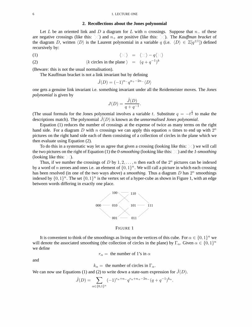
Thus, if we number the crossings ofD by 1, 2, . . . , n then each of the2n pictures can be indexedby a word ofn zeroes and ones i.e. an element of{0, 1}n. We will call a picture in which each crossinghas been resolved (in one of the two ways above) asmoothing. Thus a diagramD has2n smoothingsindexed by{0, 1}n. The set{0, 1}n is the vertex set of a hyper-cube as shown in Figure 1, with an edgebetween words differing in exactly one place.

111000 010

100

001

110

101

011

FIGURE 1

It is convenient to think of the smoothings as living on the vertices of this cube. Forα ∈ {0, 1}n wewill denote the associated smoothing (the collection of circles in the plane) byΓα. Givenα ∈ {0, 1}n

we definerα = the number of 1’s inα

andkα = the number of circles inΓα.

We can now use Equations (1) and (2) to write down a state-sum expression forJ(D).

J(D) =∑

α∈{0,1}n

(−1)rα+n−qrα+n+−2n−(q + q−1)kα .

3. THE DEFINITION OF THE KHOVANOV COMPLEX OF A LINK DIAGRAM 7

EXERCISE2.1. Convince yourself that this above state-sum formula iscorrect.

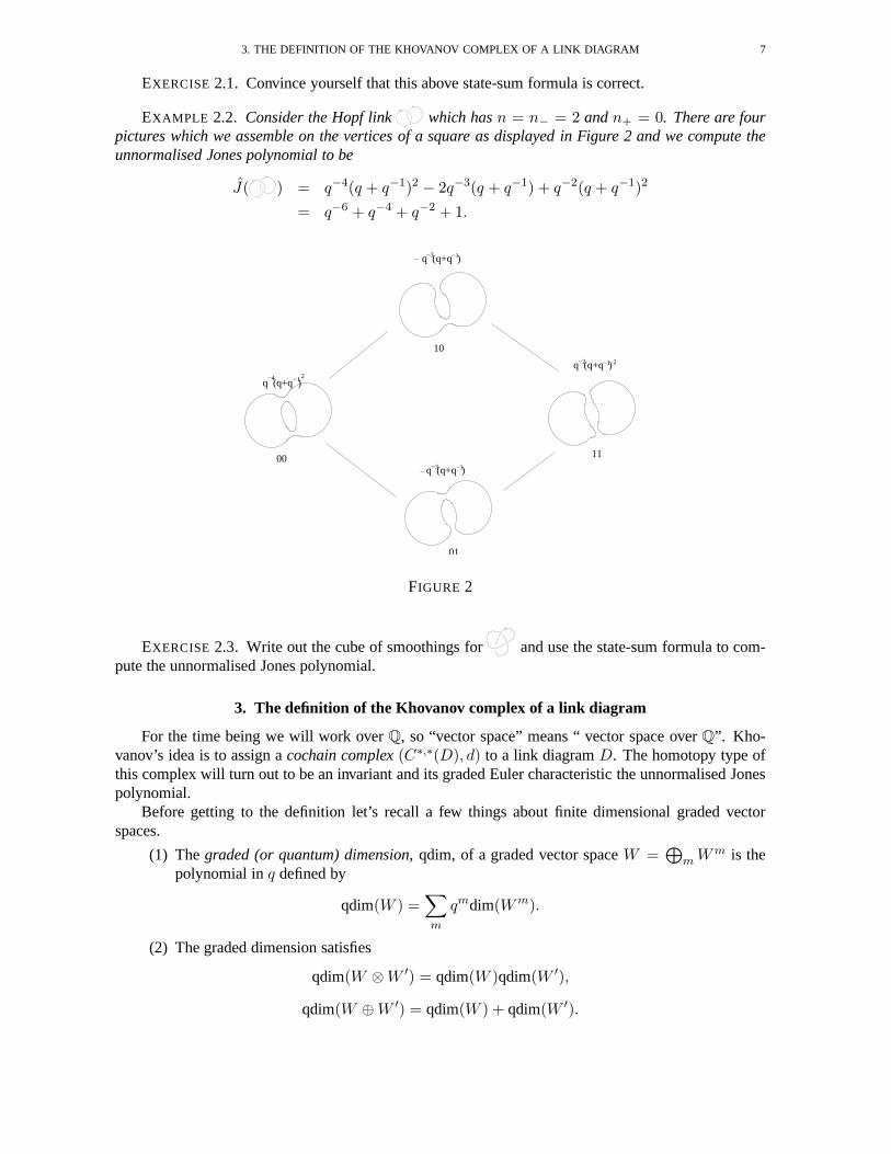
EXAMPLE 2.2. Consider the Hopf link which hasn = n− = 2 andn+ = 0. There are fourpictures which we assemble on the vertices of a square as displayed in Figure 2 and we compute theunnormalised Jones polynomial to be

J( ) = q−4(q + q−1)2 − 2q−3(q + q−1) + q−2(q + q−1)2

= q−6 + q−4 + q−2 + 1.

−1 2

10

01

1100

−2

−4 2q (q+q )−1

q (q+q )−3

−3

−1

q (q+q )−1

q (q+q )

FIGURE 2

EXERCISE 2.3. Write out the cube of smoothings for and use the state-sum formula to com-pute the unnormalised Jones polynomial.

3. The definition of the Khovanov complex of a link diagram

For the time being we will work overQ, so “vector space” means “ vector space overQ”. Kho-vanov’s idea is to assign acochain complex(C∗,∗(D), d) to a link diagramD. The homotopy type ofthis complex will turn out to be an invariant and its graded Euler characteristic the unnormalised Jonespolynomial.

Before getting to the definition let’s recall a few things about finite dimensional graded vectorspaces.

(1) Thegraded (or quantum) dimension, qdim, of a graded vector spaceW =⊕

m W m is thepolynomial inq defined by

qdim(W ) =∑

m

qmdim(W m).

(2) The graded dimension satisfies

qdim(W ⊗W ′) = qdim(W )qdim(W ′),

qdim(W ⊕W ′) = qdim(W ) + qdim(W ′).

8 1. LECTURE ONE

(3) For a graded vector spaceW and an integerl we can define a new graded vector spaceW{l}(a shifted version ofW ) by

W{l}m = W m−l

Notice that qdim(W{l}) = qlqdim(W ).

Now we turn to the definition of theKhovanov complex, C∗,∗(D), of an oriented link diagramD.An important role is played by the following two-dimensional graded vector space. LetV = Q{1, x}(theQ-vector space with basis1 andx) and grade the two basis elements by deg(1) = 1 and deg(x) =−1.

EXERCISE3.1. Show that qdim(V ⊗k) = (q + q−1)k.

Recall that we have2n smoothings of our diagram. To eachα ∈ {0, 1}n now associate the gradedvector space

Vα = V ⊗kα{rα + n+ − 2n−}

and defineCi,∗(D) =

⊕

α∈{0,1}n

rα=i+n−

Vα.

The internal grading comes from the fact that eachVα is a graded vector space. Note that the vectorspacesCi,∗(D) are trivial outside the rangei = −n−, . . . , n+.

Recall that in the last section we arranged the2n smoothings of the diagram on a cube with2n

vertices indexed by{0, 1}n. The above definition means that we now replace the smoothingΓα withthe vector spaceVα so that the spaceCi,∗(D) is the direct sum of vector spaces in columni + n− ofthe cube as indicated in Figure 3.

1111

n * n +1 * n *

V

V

V1110

1101

V1011

0111

V

V

V

V

1100

V1010

V1001

0110

0101

0011

0000V

C

V

V

V1000

0100

V0010

0001

C C

V

FIGURE 3

EXAMPLE 3.2. For the Hopf link we have the cube in Figure 4.

An element ofCi,j(D)is said to havehomological gradingi andq-gradingj. If v ∈ Vα ⊂ C∗,∗(D)with homological gradingi andq-gradingj then it is useful to remember that

i = rα − n−

j = deg(v) + i + n+ − n−

3. THE DEFINITION OF THE KHOVANOV COMPLEX OF A LINK DIAGRAM 9

V2{−4}

V{−3}

V{−3}

V{−2}

C C C−2,* −1,* 0,*

FIGURE 4

where deg(v) is the degree ofv as an element ofVα.What we need now is a differentiald turning (C∗,∗(D), d) into a complex. Recall that we have a

smoothingΓα (i.e. a collection of circles) associated to each vertexα of the cube{0, 1}n. Now to eachedge of the cube we associate acobordism(i.e. an (orientable) surface whose boundary is the union ofthe circles in the smoothings at either end).

Edges of the cube can be labelled by a string of zeroes and oneswith a star (⋆) at the position thatchanges. For example the edge joining0100 to 0110 is denoted01 ⋆ 0. We can turn edges intoarrows

by the rule:⋆ = 0 gives the tail and⋆ = 1 gives the head. For an arrowαζ

// α′ note that thesmoothingsα andα′ are identical except for a small disc (thechanging disc) around the crossing thatchanges from a 0- to a 1-smoothing (the one marked by a⋆ in ζ). For example the changing disc forthe arrowζ = 1⋆ in the cube (square!) of the Hopf link above is shown in Figure5.

FIGURE 5

10 1. LECTURE ONE

The cobordismWζ associated toαζ

// α′ is defined to be the following surface: outside thechanging disc take the product ofΓα with the unit interval and then plug the missing tube with the

saddle Thus eachWζ consists of a bunch of cylinders and one pair-of-pants surface ( or ).

Cobordism convention: pictures of cobordisms godownthe page.

Above we replaced the smoothingΓα by the vector spaceVα and now we will replace the cobor-

dism Wζ associated to the edgeαζ

// α′ by a linear mapdζ : Vα → Vα′ . Since each circle in asmoothing has a copy of the vector spaceV attached to it, to definedζ we only require two linearmaps: one that fusesm : V ⊗ V → V and one that splits∆: V → V ⊗ V . Then we can definedζ tobe the identity on circles not entering the changing disc andeitherm or ∆ on the circles appearing inthe changing disc (depending on whether the pair-of-pants has two or one input boundary circles).

We definem : V ⊗ V → V by

12 = 1, 1x = x1 = x, x2 = 0,

and∆: V → V ⊗ V by

∆(1) = 1⊗ x + x⊗ 1, ∆(x) = x⊗ x.

In fact by defining a uniti(1) = 1 and counitǫ(1) = 0 andǫ(x) = 1 we have endowedV withthe structure of a commutativeFrobenius algebra. Isomorphism classes of commutative Frobeniusalgebras are in bijective correspondence with isomorphisms classes of 1+1-dimensional topologicalquantum field theories so what we are really doing here is applying a TQFT (the one defined byV ) tothe cube of circles and cobordisms - more on this in Lecture 2.

We are finally ready to definedi : Ci,∗(D)→ Ci+1,∗(D). Forv ∈ Vα ⊂ Ci,∗(D) set

di(v) =∑

ζ such thatTail(ζ)=α

sign(ζ)dζ(v)

where sign(ζ) = (−1)number of 1’s to the left of⋆ in ζ .

PROPOSITION3.3. di+1 ◦ di = 0.

PROOF. (sketch) The idea of the proof is that without the signs eachface of the cube commutes. Tosee this one can either look at a number of cases and use the definition of the mapsm and∆ or (muchbetter) begin to think geometrically: each of the two routesaround a face gives the same cobordism (upto homeomorphism) and so applying the TQFT defined byV gives the same linear map. Once all thenon-signed faces commute then observe that the signs occur in odd numbers on every face, thus turningcommutativity into anti-commutativity. �

EXERCISE 3.4. Write out the above proof properly - you may wish to wait until after Lecture 2where there is a more detailed discussion of Frobenius algebras and TQFTs.

EXERCISE3.5. Check thatd has bi-grading(1, 0).

The graded Euler characteristic of this complex i.e.∑

(−1)iqdim(Ci,∗(D)) ∈ Q[q±1]

is nothing other than the unnormalised Jones polynomial.

EXERCISE 3.6. Convince yourself that the previous statement is true -this is simply a matter ofunwinding the definitions and then comparing with the state-sum formula for the unnormalised Jonespolynomial.

4. NOTES AND FURTHER READING 11

Later we will see that the homotopy type of(C∗,∗(D), d) is invariant under transformations byReidemeister moves. For now, to end this lecture, let us perform a homology calculation.

EXAMPLE 3.7. Let us compute thehomologyofC∗,∗( ). The complex has only three non-trivialterms:

0 // C−2,∗(D)d

// C−1,∗(D)d

// C0,∗(D) // 0.

More explicitly we have:

V {−3}−∆

''NNNNNNNNNNN

(V ⊗ V ){−4}

m77ppppppppppp

m''NNNNNNNNNNN⊕ (V ⊗ V ){−2}

V {−3}

∆77ppppppppppp

and based on this one can compute as follows.

Homological degree -2 -1 0Cycles {1⊗ x− x⊗ 1, x⊗ x} {(1, 1), (x, x)} {1⊗ 1, 1⊗ x, x⊗ 1, x⊗ x}Boundaries - {(1, 1), (x, x)} {1⊗ x + x⊗ 1, x⊗ x}Homology {1⊗ x− x⊗ 1, x⊗ x} - {1⊗ 1, 1 ⊗ x}q-degrees -4, -6 0, -2

The homology can be summarised as a table where the homological degree is horizontal and theq-degree vertical.

ji

-2 -1 0

0 Q

-1-2 Q

-3-4 Q

-5-6 Q

EXERCISE 3.8. Write out the cube for the trefoil explicitly (including the correct signs on theedges). Calculate the homology of the Khovanov complex. This involves a bit of work, but is a verygood test to see if you have understood all the definitions.

4. Notes and further reading

The original paper by Khovanov in which he defines the complexand establishes the basic propertiesis [Khovanov1]. In this paper he starts out working over the ringZ[c] and then setsc = 0 to work overZ. We work overQ because some things are a little simpler. We will say more about other coefficientsin Lecture 3. Bar-Natan’s exposition of Khovanov’s work [Bar-Natan2] is extremely readable and hasalso been very influential.

CHAPTER 2

Lecture Two

The complexC∗,∗(D) for a link diagramD defined in Lecture 1 depends very much on the dia-gram. However, it turns out that different diagrams for the same link give complexes which arehomo-topy equivalent. In this lecture we begin with an aside on Frobenius algebrasand topological quantumfield theories and after this discuss the homotopy invariance properties of the Khovanov complex con-centrating on the first Reidemeister move. Finally in this lecture we define Khovanov homology anddiscuss some properties.

1. Frobenius algebras and TQFTs

Hidden in the background in Lecture 1, about to come to deserved prominence, are 1+1-dimensionaltopological quantum field theories and their algebraic counterparts, Frobenius algebras.

A commutative Frobenius algebra overR (a commutative ring with unit) is a unital, commutativeR-algebraV which as anR-module is projective of finite type (ifR = Q this just means a finitedimensional vector space overQ), together with a module homomorphism, the counit,ǫ : V → R suchthat the bilinear form〈−,−〉 : V ⊗ V → R defined by〈v,w〉 = ǫ(vw) is non-degenerate i.e. theadjoint homomorphismV → V ∗ is an isomorphism. It is useful to define a coproduct∆: V → V ⊗Vby ∆(v) =

∑

i v′i ⊗ v′′i being the unique element such that for allw ∈ V , vw =

∑

i v′i〈v′′i , w〉.

Frobenius algebras reflect the topology of surfaces. This statement is the rough equivalent of themore accurate:

{Iso. classes of comm. Frobenius algebras} ←→ {Iso. classes of 1+1-dimensional TQFTs}

Recall that a 1+1-dimensional TQFT is a monoidal functorCob1+1 → ModR whereCob1+1 is thecategory whose objects are closed, oriented 1-manifolds and where a morphismΓ→ Γ′ is an orientedsurfaceW with ∂W = Γ⊔ Γ′ (here the overline means take the opposite orientation). Infact you haveto be careful to get the details of all this right - see the references at the end of the lecture. The upshotis that a TQFT:

• assigns to each closed 1-manifoldΓ, anR-moduleVΓ such that ifΓ = Γ0 ⊔ Γ1 thenVΓ =VΓ0⊗ VΓ1

(this what the adjective “monoidal” refers to) and• assigns to each cobordismW : Γ→ Γ′, anR-homomorphismVΓ → VΓ′ .

These assignments are subject to some axioms which, among other things, guarantee

• homeomorphic cobordisms induce the same homomorphism,• gluing of cobordisms is well behaved, and• V∅ = R.

Using the correspondence between Frobenius algebras and 1+1-dimensional TQFTs one can usethe topology to prove algebraic statements. For example, for any Frobenius algebra one can checkthat m(∆(v)) = m(m(∆(1)), v) for all v ∈ V . Checking this algebraically is a bit of a pain, butgeometrically it is a triviality: the two surfaces in Figure1 are homeomorphic and therefore correspondto the same homomorphism of Frobenius algebras.

In Lecture 1 we defined a particular two dimensional Frobenius algebraV which, by the above,defines a 1+1-dimensional TQFT. Given a link diagram we considered the cube{0, 1}n and associatedto each vertexα a collection of circlesΓα (a smoothing) and to each edgeζ a cobordismWζ . In order

13

14 2. LECTURE TWO

FIGURE 1

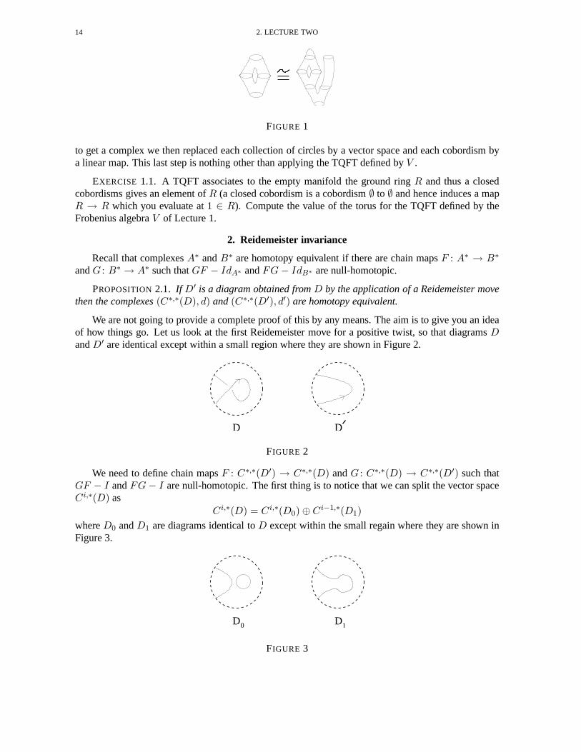
to get a complex we then replaced each collection of circles by a vector space and each cobordism bya linear map. This last step is nothing other than applying the TQFT defined byV .

EXERCISE 1.1. A TQFT associates to the empty manifold the ground ringR and thus a closedcobordisms gives an element ofR (a closed cobordism is a cobordism∅ to ∅ and hence induces a mapR → R which you evaluate at1 ∈ R). Compute the value of the torus for the TQFT defined by theFrobenius algebraV of Lecture 1.

2. Reidemeister invariance

Recall that complexesA∗ andB∗ are homotopy equivalent if there are chain mapsF : A∗ → B∗

andG : B∗ → A∗ such thatGF − IdA∗ andFG− IdB∗ are null-homotopic.

PROPOSITION2.1. If D′ is a diagram obtained fromD by the application of a Reidemeister movethen the complexes(C∗,∗(D), d) and(C∗,∗(D′), d′) are homotopy equivalent.

We are not going to provide a complete proof of this by any means. The aim is to give you an ideaof how things go. Let us look at the first Reidemeister move fora positive twist, so that diagramsDandD′ are identical except within a small region where they are shown in Figure 2.

DD

FIGURE 2

We need to define chain mapsF : C∗,∗(D′) → C∗,∗(D) andG : C∗,∗(D) → C∗,∗(D′) such thatGF − I andFG− I are null-homotopic. The first thing is to notice that we can split the vector spaceCi,∗(D) as

Ci,∗(D) = Ci,∗(D0)⊕ Ci−1,∗(D1)

whereD0 andD1 are diagrams identical toD except within the small regain where they are shown inFigure 3.

1D D0

FIGURE 3

2. REIDEMEISTER INVARIANCE 15

EXERCISE 2.2. Understand why there is the shift forD1 in the above decomposition. What hap-pens to theq-grading?

The differentiald can be written with respect to this splitting as a matrix

(

d0 0δ d1

)

.

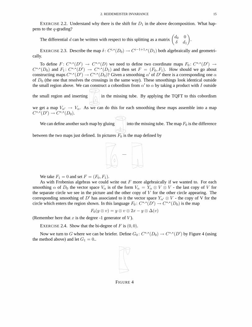
EXERCISE2.3. Describe the mapδ : Ci,∗(D0)→ Ci−1+1,∗(D1) both algebraically and geometri-cally.

To defineF : C∗,∗(D′) → C∗,∗(D) we need to define two coordinate mapsF0 : C∗,∗(D′) →C∗,∗(D0) and F1 : C∗,∗(D′) → C∗,∗(D1) and then setF = (F0, F1). How should we go aboutconstructing mapsC∗,∗(D′)→ C∗,∗(D0)? Given a smoothingα′ of D′ there is a corresponding oneαof D0 (the one that resolves the crossings in the same way). These smoothings look identical outsidethe small region above. We can construct a cobordism fromα′ to α by taking a product withI outside

the small region and inserting in the missing tube. By applying the TQFT to this cobordism

we get a mapVα′ → Vα. As we can do this for each smoothing these maps assemble intoa mapC∗,∗(D′)→ C∗,∗(D0).

We can define another such map by gluing into the missing tube. The mapF0 is the difference

between the two maps just defined. In picturesF0 is the map defined by

We takeF1 = 0 and setF = (F0, F1).As with Frobenius algebras we could write outF more algebraically if we wanted to. For each

smoothingα of D0 the vector spaceVα is of the formVα = Yα ⊗ V ⊗ V - the last copy ofV forthe separate circle we see in the picture and the other copy ofV for the other circle appearing. Thecorresponding smoothing ofD′ has associated to it the vector spaceYα′ ⊗ V - the copy of V for thecircle which enters the region shown. In this languageF0 : C∗,∗(D′)→ C∗,∗(D0) is the map

F0(y ⊗ v) = y ⊗ v ⊗ 2x− y ⊗∆(v)

(Remember here thatx is the degree -1 generator ofV ).

EXERCISE2.4. Show that the bi-degree ofF is (0, 0).

Now we turn toG where we can be briefer. DefineG0 : C∗,∗(D0)→ C∗,∗(D′) by Figure 4 (usingthe method above) and letG1 = 0..

FIGURE 4

16 2. LECTURE TWO

EXERCISE2.5. So farF andG are maps of vector spaces: check they are chain maps.

We now claim thatG andF are part of a homotopy equivalence i.e. thatGF − I is null homotopicandFG− I is null homotopic.

For the first of these we claimGF = I (showingGF −I is null homotopic via a trivial homotopy).This is where using pictures comes into its own: the picture for the compositionGF is simply gottenby placing one picture on top of the other as seen in Figure 5.

GF 2 I

FIGURE 5

Next we claim there is a mapH : C∗,∗(D) → C∗−1,∗(D) such thatFG − I = Hd + dH. Using

the splitting aboveH is the matrix

(

0 h0 0

)

where−h : C∗,∗(D1) → C∗,∗(D0) is the map gotten by

the method above using the picture

We computeHd + dH =

(

hδ hd1 + d0h0 δh

)

. Thus we need to show

hδ = F0G0 − I(3)

hd1 + d0h = 0(4)

δh = −I(5)

Equation (5) is easy: just compose pictures as shown in Figure 6.

FIGURE 6

Equation (4) is essentially just due to the fact thatd0 andd1 are defined using the same cobordism(for d0 there is an extra cylinder) and by then looking carefully at the signs in the definition of thedifferential.

EXERCISE2.6. Check the assertions of the previous sentence.

3. KHOVANOV HOMOLOGY 17

Pictorially (3) is shown in Figure 7. I know of no enlightening way to do it, but it is a simple matterto see that this holds forV . (Remember the cobordism is the identity outside the regionso we need tocheck the equality for mapsV ⊗ V → V ⊗ V .)

FIGURE 7

This concludes invariance under Reidemeister I positive twist: we have producedF andG suchthatFG− I andGF − I are null-homotopic, thus demonstrating that there is a homotopy equivalenceC∗,∗(D′) ≃ C∗,∗(D).

The above essentially follows Bar-Natan’s proof - though Bar-Natan is cleverer still: in his set-up one constructs ageometriccomplex and works with tangles. One proves invariance without everapplying a TQFT. This gives rise to auniversal theory- more on this in the next lecture. Refer to theend of the lecture for further remarks and a reference.

3. Khovanov homology

Given an oriented link diagramD we now define theKhovanov homology of the diagramD by

KH∗,∗(D) = H(C∗,∗(D), d).

By the previous section ifD is related toD′ by a series of Reidemeister moves then there is an iso-morphismKH∗,∗(D) ∼= KH∗,∗(D′). Thus if L is an oriented link it makes sense to talk about theKhovanov homology of the linkL (defined up to isomorphism as the Khovanov homology of any dia-gram representing it).

PROPOSITION3.1.∑

(−1)iqdim(KH i,∗(L)) = J(L)

PROOF. It is an exercise in linear algebra to show that∑

(−1)iqdim(KH i,∗(D)) =∑

(−1)iqdim(Ci,∗(D))

and we have already observed that the right-hand side isJ(L). �

Khovanov homology is a stronger invariant than the Jones polynomial as the following exampleillustrates.

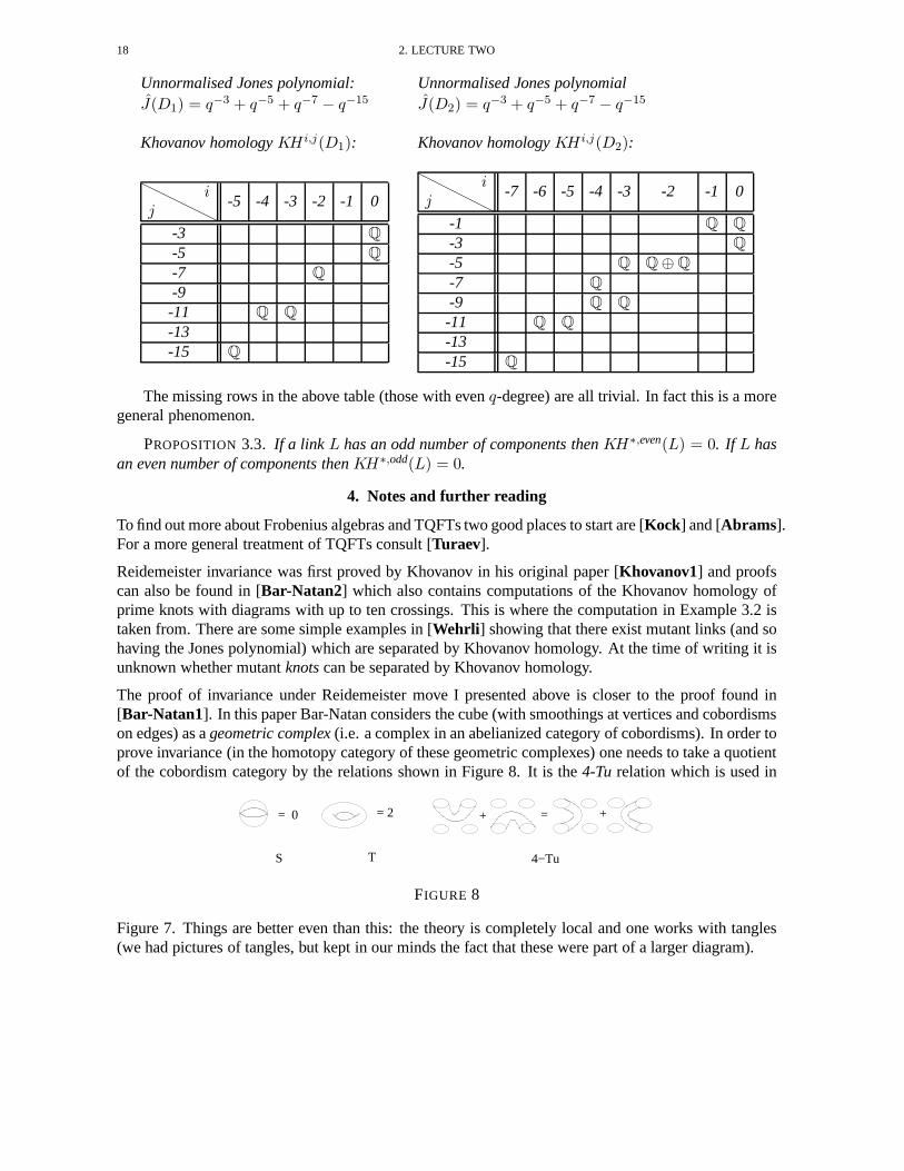
EXAMPLE 3.2.

D1 = D2 =

18 2. LECTURE TWO

Unnormalised Jones polynomial: Unnormalised Jones polynomialJ(D1) = q−3 + q−5 + q−7 − q−15 J(D2) = q−3 + q−5 + q−7 − q−15

Khovanov homologyKH i,j(D1): Khovanov homologyKH i,j(D2):

ji

-5 -4 -3 -2 -1 0

-3 Q

-5 Q

-7 Q

-9-11 Q Q

-13-15 Q

ji

-7 -6 -5 -4 -3 -2 -1 0

-1 Q Q

-3 Q

-5 Q Q⊕Q

-7 Q

-9 Q Q

-11 Q Q

-13-15 Q

The missing rows in the above table (those with evenq-degree) are all trivial. In fact this is a moregeneral phenomenon.

PROPOSITION3.3. If a link L has an odd number of components thenKH∗,even(L) = 0. If L hasan even number of components thenKH∗,odd(L) = 0.

4. Notes and further reading

To find out more about Frobenius algebras and TQFTs two good places to start are [Kock] and [Abrams].For a more general treatment of TQFTs consult [Turaev].

Reidemeister invariance was first proved by Khovanov in his original paper [Khovanov1] and proofscan also be found in [Bar-Natan2] which also contains computations of the Khovanov homologyofprime knots with diagrams with up to ten crossings. This is where the computation in Example 3.2 istaken from. There are some simple examples in [Wehrli ] showing that there exist mutant links (and sohaving the Jones polynomial) which are separated by Khovanov homology. At the time of writing it isunknown whether mutantknotscan be separated by Khovanov homology.

The proof of invariance under Reidemeister move I presentedabove is closer to the proof found in[Bar-Natan1]. In this paper Bar-Natan considers the cube (with smoothings at vertices and cobordismson edges) as ageometric complex(i.e. a complex in an abelianized category of cobordisms). In order toprove invariance (in the homotopy category of these geometric complexes) one needs to take a quotientof the cobordism category by the relations shown in Figure 8.It is the4-Tu relation which is used in

S

= 0 = 2 + = +

4−TuT

FIGURE 8

Figure 7. Things are better even than this: the theory is completely local and one works with tangles(we had pictures of tangles, but kept in our minds the fact that these were part of a larger diagram).

CHAPTER 3

Lecture Three

In this lecture we begin by looking at a long exact sequence inKhovanov homology. Then weexamine the kind of functoriality present and briefly discuss the invariants of embedded surfaces inR4

thus defined. We end with a look at theories defined over different base rings.

1. A long exact sequence

In algebraic topology there are many theoretical tools for computation such as long exact se-quences, spectral sequence and so on. In Khovanov homology there is less available in the arsenal,but there is one useful long exact sequence which we now discuss.

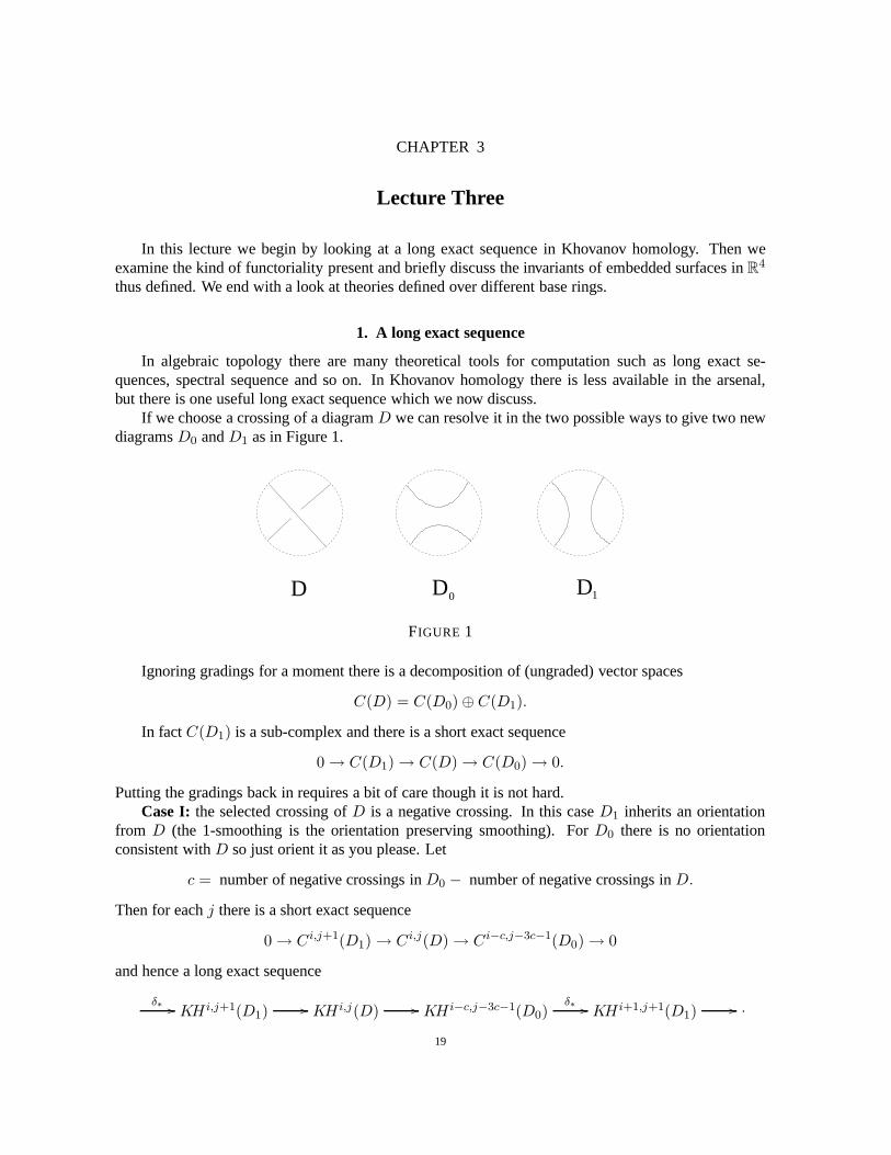
If we choose a crossing of a diagramD we can resolve it in the two possible ways to give two newdiagramsD0 andD1 as in Figure 1.

1D D D0

FIGURE 1

Ignoring gradings for a moment there is a decomposition of (ungraded) vector spaces

C(D) = C(D0)⊕ C(D1).

In factC(D1) is a sub-complex and there is a short exact sequence

0→ C(D1)→ C(D)→ C(D0)→ 0.

Putting the gradings back in requires a bit of care though it is not hard.Case I: the selected crossing ofD is a negative crossing. In this caseD1 inherits an orientation

from D (the 1-smoothing is the orientation preserving smoothing). For D0 there is no orientationconsistent withD so just orient it as you please. Let

c = number of negative crossings inD0 − number of negative crossings inD.

Then for eachj there is a short exact sequence

0→ Ci,j+1(D1)→ Ci,j(D)→ Ci−c,j−3c−1(D0)→ 0

and hence a long exact sequence

δ∗// KH i,j+1(D1) // KH i,j(D) // KH i−c,j−3c−1(D0)

δ∗// KH i+1,j+1(D1) // .

19

20 3. LECTURE THREE

If we write the differential ofC∗,∗(D) as a matrix

(

d0 0δ d1

)

then the boundary map in the long

exact sequence isδ∗ i.e. the map induced in homology (suitably shifted to take account of the neworientation ofD0).

Case II: the selected crossing ofD is a positive crossing. In this caseD0 inherits an orienta-tion from D (this time the 0-smoothing is the orientation preserving smoothing). ForD1 there is noorientation consistent withD so just orient it as you please. Let

c = number of negative crossings inD1 − number of negative crossings inD.

Then for eachj there is a short exact sequence

0→ Ci−c−1,j−3c−2(D1)→ Ci,j(D)→ Ci,j−1(D0)→ 0

and hence a long exact sequence

δ∗// KH i−c−1,j−3c−2(D1) // KH i,j(D) // KH i,j−1(D0)

δ∗// KH i−c,j−3c−2(D1) // .

EXERCISE1.1. Check the gradings in the long exact sequences above.

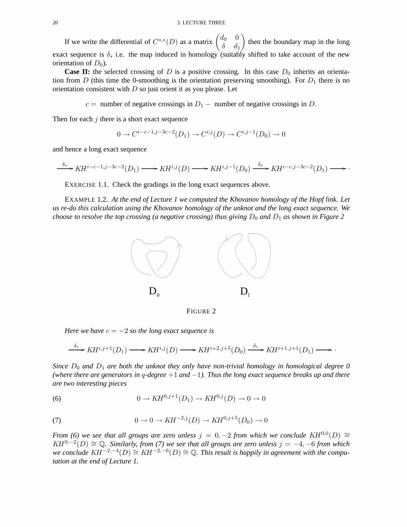
EXAMPLE 1.2. At the end of Lecture 1 we computed the Khovanov homology of the Hopf link. Letus re-do this calculation using the Khovanov homology of theunknot and the long exact sequence. Wechoose to resolve the top crossing (a negative crossing) thus givingD0 andD1 as shown in Figure 2

0 D1D

FIGURE 2

Here we havec = −2 so the long exact sequence is

δ∗// KH i,j+1(D1) // KH i,j(D) // KH i+2,j+5(D0)

δ∗// KH i+1,j+1(D1) // .

SinceD0 and D1 are both the unknot they only have non-trivial homology in homological degree 0(where there are generators inq-degree+1 and−1). Thus the long exact sequence breaks up and thereare two interesting pieces

(6) 0→ KH0,j+1(D1)→ KH0,j(D)→ 0→ 0

(7) 0→ 0→ KH−2,j(D)→ KH0,j+5(D0)→ 0

From (6) we see that all groups are zero unlessj = 0,−2 from which we concludeKH0,0(D) ∼=KH0,−2(D) ∼= Q. Similarly, from (7) we see that all groups are zero unlessj = −4,−6 from whichwe concludeKH−2,−4(D) ∼= KH−2,−6(D) ∼= Q. This result is happily in agreement with the compu-tation at the end of Lecture 1.

2. FUNCTORIAL PROPERTIES 21

2. Functorial properties

It is convenient to study links by projecting onto the plane and studying link diagrams instead.The diagrammatic representation of a given link is far from unique, but this is well understood: twodiagrams represent the isotopic links if and only if they arerelated by Reidemeister moves.

Something similar is true for link cobordisms (recall that alink cobordism(Σ, L0, L1) is a smooth,compact, oriented surfaceΣ generically embedded inR3 × I such that∂Σ = L0 ⊔ L1 with ∂Σ ⊂R3 × {0, 1}). A link cobordism can be represented by a sequence of oriented link diagrams - the firstin the sequence being a diagramD0 for L0 and the last being a diagramD1 for L1. Two consecutivediagrams in this sequence must be related by a small set of allowable moves which are

(1) Reidemeister I, II or III moves,(2) Morse 0-,1- or 2-handle moves.

The Reidemeister moves are just the usual ones and the Morse moves are shown in Figure 3.

2−handle0−handle 1−handle

FIGURE 3

Geometrically the Morse moves are shown in Figure 4.

2−handle0−handle 1−handle

FIGURE 4

Such a sequence of diagrams is known as amovie.

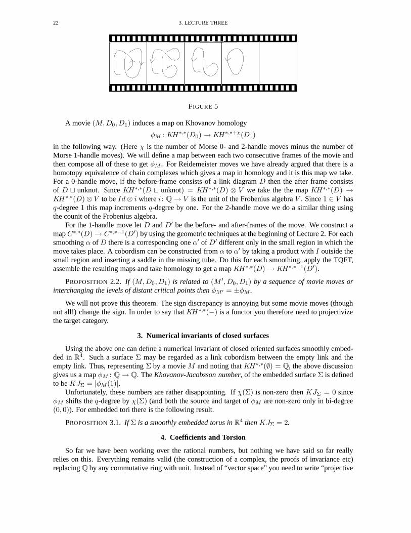
EXAMPLE 2.1. Figure 5 is a movie representing a cobordism from the Hopf link to the emptycobordism (drawn across the page rather than down to save space).

A movie representation of a link cobordism is not unique: there may be many different moviesof the same cobordism. However, again this is well understood: two movies represent isotopic linkcobordisms if and only if they are related by a series ofmovie movesor by interchanging the levels ofdistant critical points. Each movie move replaces a small clip of the movie by a different clip. We willnot go into this in more detail here.

22 3. LECTURE THREE

FIGURE 5

A movie (M,D0,D1) induces a map on Khovanov homology

φM : KH∗,∗(D0)→ KH∗,∗+χ(D1)

in the following way. (Hereχ is the number of Morse 0- and 2-handle moves minus the number ofMorse 1-handle moves). We will define a map between each two consecutive frames of the movie andthen compose all of these to getφM . For Reidemeister moves we have already argued that there isahomotopy equivalence of chain complexes which gives a map inhomology and it is this map we take.For a 0-handle move, if the before-frame consists of a link diagramD then the after frame consistsof D ⊔ unknot. SinceKH∗,∗(D ⊔ unknot) = KH∗,∗(D) ⊗ V we take the the mapKH∗,∗(D) →KH∗,∗(D)⊗ V to beId⊗ i wherei : Q→ V is the unit of the Frobenius algebraV . Since1 ∈ V hasq-degree 1 this map incrementsq-degree by one. For the 2-handle move we do a similar thing usingthe counit of the Frobenius algebra.

For the 1-handle move letD andD′ be the before- and after-frames of the move. We construct amapC∗,∗(D)→ C∗,∗−1(D′) by using the geometric techniques at the beginning of Lecture 2. For eachsmoothingα of D there is a corresponding oneα′ of D′ different only in the small region in which themove takes place. A cobordism can be constructed fromα to α′ by taking a product withI outside thesmall region and inserting a saddle in the missing tube. Do this for each smoothing, apply the TQFT,assemble the resulting maps and take homology to get a mapKH∗,∗(D)→ KH∗,∗−1(D′).

PROPOSITION2.2. If (M,D0,D1) is related to(M ′,D0,D1) by a sequence of movie moves orinterchanging the levels of distant critical points thenφM ′ = ±φM .

We will not prove this theorem. The sign discrepancy is annoying but some movie moves (thoughnot all!) change the sign. In order to say thatKH∗,∗(−) is a functor you therefore need to projectivizethe target category.

3. Numerical invariants of closed surfaces

Using the above one can define a numerical invariant of closedoriented surfaces smoothly embed-ded inR4. Such a surfaceΣ may be regarded as a link cobordism between the empty link andtheempty link. Thus, representingΣ by a movieM and noting thatKH∗,∗(∅) = Q, the above discussiongives us a mapφM : Q→ Q. TheKhovanov-Jacobsson number, of the embedded surfaceΣ is definedto beKJΣ = |φM (1)|.

Unfortunately, these numbers are rather disappointing. Ifχ(Σ) is non-zero thenKJΣ = 0 sinceφM shifts theq-degree byχ(Σ) (and both the source and target ofφM are non-zero only in bi-degree(0, 0)). For embedded tori there is the following result.

PROPOSITION3.1. If Σ is a smoothly embedded torus inR4 thenKJΣ = 2.

4. Coefficients and Torsion

So far we have been working over the rational numbers, but nothing we have said so far reallyrelies on this. Everything remains valid (the constructionof a complex, the proofs of invariance etc)replacingQ by any commutative ring with unit. Instead of “vector space”you need to write “projective

4. COEFFICIENTS AND TORSION 23

R-module of finite type”. In particular you can work over the integers and ask if, like for ordinaryhomology of spaces, the interesting phenomenon oftorsionemerges. It does.

The first place this is seen is for the trefoil . The cube of this trefoil (as requested in the exerciseat the end of Lecture 1) is given in Figure 6.

*C C C C−3 −2 −1 0* **

1

2

000

100

010

001

110

101

011

111

3

FIGURE 6

In bi-degree(−2,−7) the cycles are generated by

{z1 = (x⊗ x, 0, 0), z2 = (0, x⊗ x, 0), z3 = (0, 0, x ⊗ x)}

and in bi-degree(−3,−7) the chains are generated by

{c1 = (1, x, x), c2 = (x, 1, x), c3 = (x, x, 1)}.

Recalling the definition of the differential one easily sees

d(c1) = z1 + z3 d(c2) = z2 + z3 d(c3) = z1 + z2

Thus in homology we have[z1] = [z2] = [z3]. Note also that

d(c1 + c3 − c2) = z1 + z3 + z1 + z2 − z2 − z3 = 2z1.

Thus, rationallyz1 is a boundary (it is hit by12(c1 + c3 − c2)) and our potential homology class aboveis trivial. Over the integers[z1] is a non-trivial homology class, but2[z1] is trivial, thus in homologywe have a copy ofZ/2.

For the record the full integral homology of the trefoil is given below.

ji

-3 -2 -1 0

-1 Z

-3 Z

-5 Z

-7 Z/2-9 Z

In fact torsion abounds as shown in the following result (which we do not prove):

24 3. LECTURE THREE

PROPOSITION4.1. The integral Khovanov homology of every alternating link, except the trivialknot, the Hopf link and their connected sums and disjoint unions, has torsion of order two.

In order to describe Khovanov homology with coefficients in aring R in terms of integral Khovanovhomology we apply a standard result in homological algebra:the universal coefficient theorem. SinceC∗,∗(D;R) = C∗,∗(D; Z) ⊗Z R the universal coefficient theorem tells us that there is a short exactsequence

0 // KH i,j(D; Z)⊗Z R // KH i,j(D;R) // Tor(KH i+1,j(D; Z), R) // 0.

EXERCISE4.2. Use the short exact sequence above to computeKH∗,∗( ; Z/2).

Closely related to this is the Kunneth formula, which we canuse to compute the Khovanov ho-mology of a disjoint union. Given two link diagramsD1 andD2 thenC∗,∗(D1 ⊔D2) ∼= C∗,∗(D1) ⊗C∗,∗(D2) or more precisely:

Ci,j(D1 ⊔D2) ∼=⊕

p+q=is+t=j

Cp,s(D1)⊗ Cq,t(D2).

Thus the Kunneth formula gives us a split short exact sequence

0→⊕

p+q=is+t=j

KHp,s(D1;R)⊗KHq,t(D2;R)→ KH i,j(D1 ⊔D2;R)

→⊕

p+q=i+1s+t=j

TorR1 (KHp,s(D1;R),⊗KHq,t(D2;R))→ 0.

OverQ the Tor group is always trivial so we have

KH i,j(D1 ⊔D2; Q) ∼=⊕

p+q=is+t=j

KHp,s(D1; Q)⊗KHq,t(D2; Q).

5. Notes and further reading

The long exact sequence is implicit in Khovanov’s original paper, but appeared in a slightly differentform in [Viro ]. Lee used the singly graded version in [Lee]. It has appeared in a variety of places sincethen and with gradings as we have given them in [Rasmussen4]. This is an interesting survey paper inits own right discussing parallels between Khovanov homology and knot Floer homologies.

You can read about, cobordisms and their representations asmovies in [CarterSaito].

Khovanov conjectured the functoriality properties in his original paper [Khovanov1]. This was thenproved in [Jacobsson] and independently in [Khovanov2]. Using his geometric techniques Bar-Natanproved functoriality (in more generality) in [Bar-Natan1].

The proposition about Khovanov-Jacobsson numbers has beenproved for a certain class of torus em-beddings in [CarterSaitoSatoh] and then for all torus embeddings in [Tanaka] and independentlyusing different techniques in [Rasmussen2].

Torsion in Khovanov homology has been studied in a number of papers. The best places to start wouldbe [Shumakovitch] and [AsaedaPrzytycki]. Both of these prove Proposition 4.1 concerning 2-torsionand the former has a number of interesting conjectures abouttorsion. One of these conjectures thatall torsion is 2-torsion, which is now known to be false. Bar-Natan’s computer program calculatesKH22,73(T (8, 7)) = Z/2 ⊕ Z/4 ⊕ Z/5 ⊕ Z/7, whereT (8, 7) is the torus link with 7 strands and 8positive twists.

CHAPTER 4

Lecture Four

In this lecture we begin by discussing a family of Khovanov-type link homology theories, thenfocus on the first of these to be defined, Lee theory. This naturally leads to the work of Rasmussen ona new concordance invariant of knots which has many wonderful properties.

1. A family of Khovanov-type theories

An obvious question to ask is: can we replace the Frobenius algebraV used to construct theKhovanov complex by some other Frobenius algebra and still get a link homology theory (i.e. aninvariant with nice functorial properties)? Or, re-phrased, what conditions must a Frobenius algebraAsatisfy to give a link homology theory?

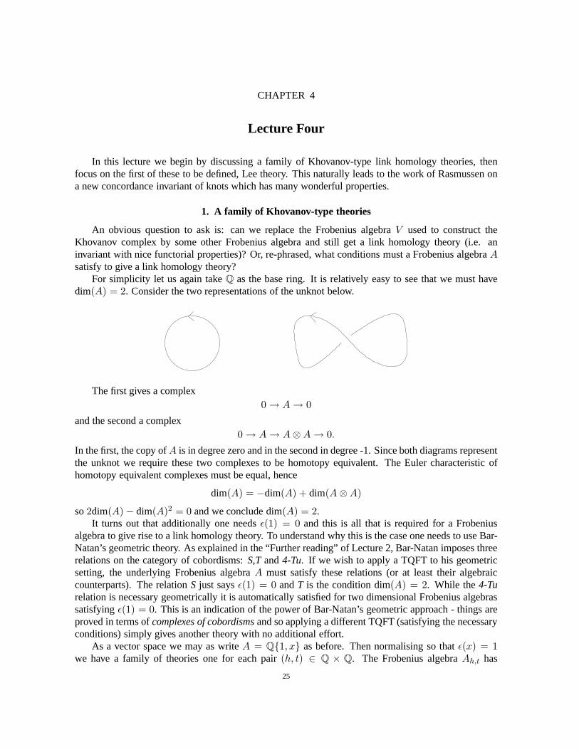
For simplicity let us again takeQ as the base ring. It is relatively easy to see that we must havedim(A) = 2. Consider the two representations of the unknot below.

The first gives a complex0→ A→ 0

and the second a complex0→ A→ A⊗A→ 0.

In the first, the copy ofA is in degree zero and in the second in degree -1. Since both diagrams representthe unknot we require these two complexes to be homotopy equivalent. The Euler characteristic ofhomotopy equivalent complexes must be equal, hence

dim(A) = −dim(A) + dim(A⊗A)

so2dim(A)− dim(A)2 = 0 and we conclude dim(A) = 2.It turns out that additionally one needsǫ(1) = 0 and this is all that is required for a Frobenius

algebra to give rise to a link homology theory. To understandwhy this is the case one needs to use Bar-Natan’s geometric theory. As explained in the “Further reading” of Lecture 2, Bar-Natan imposes threerelations on the category of cobordisms:S,Tand4-Tu. If we wish to apply a TQFT to his geometricsetting, the underlying Frobenius algebraA must satisfy these relations (or at least their algebraiccounterparts). The relationS just saysǫ(1) = 0 andT is the condition dim(A) = 2. While the4-Turelation is necessary geometrically it is automatically satisfied for two dimensional Frobenius algebrassatisfyingǫ(1) = 0. This is an indication of the power of Bar-Natan’s geometricapproach - things areproved in terms ofcomplexes of cobordismsand so applying a different TQFT (satisfying the necessaryconditions) simply gives another theory with no additionaleffort.

As a vector space we may as writeA = Q{1, x} as before. Then normalising so thatǫ(x) = 1we have a family of theories one for each pair(h, t) ∈ Q × Q. The Frobenius algebraAh,t has

25

26 4. LECTURE FOUR

multiplication given by12 = 1 1x = x1 = x x2 = hx + t1

and comultiplication given by

∆(1) = 1⊗ x + x⊗ 1− h1⊗ 1 ∆(x) = x⊗ x + t1⊗ 1.

The unit and counit arei(1) = 1 ǫ(1) = 0 ǫ(x) = 1.

A link homology theory is obtained by carrying out exactly the same construction as outlined in Lecture1, but replacing the Frobenius algebraV with Ah,t. Whenh = t = 0 then you get the original theoryof Lecture 1.

The first such variant to be studied was the case(h, t) = (0, 1) by E.S. Lee giving a theory nowknown asLee Theory- the topic of the next section.

In fact, up to isomorphism Lee theory is the only other rational theory in the family under discus-sion.

PROPOSITION1.1. If h2 +4t = 0 then the resulting theory is isomorphic to the original Khovanovhomology and ifh2 + 4t 6= 0 then the resulting theory is isomorphic to Lee theory.

2. Lee theory

The alert reader will have noticed a minor problem in carrying out the construction in Lecture 1using the Frobenius algebraAh,t. This is that one loses theq-grading. The degree ofx2 = hx + t1is not even homogeneous ifh andt are both non-zero. In fact the only case where a second gradingexists ish = t = 0. For now let us simply ignore theq-grading: all theories will be singly graded bythe homological grading. In the next section we will see thatin fact that we do not need to completelythrow away the second grading - it just gets replaced by a filtration instead.

Lee theory (h = 0, t = 1) was the first variant of Khovanov homology to appear and remarkably itcan be computed explicitly.

PROPOSITION2.1. The dimension ofLee∗(L) is 2k wherek is the number of components inL.

Things are even better still and there are explicit generators whose construction is as follows. Thereare2k possible orientations ofL. Given an orientationθ there is acanonical smoothingobtained bysmoothing all positive crossings to 0-smoothings and all negative crossings to 1-smoothings. For thissmoothing one can divide the circles into two disjoint groups, Group 0 and Group 1 as follows. A circlebelongs to Group 0 (Group 1) if it has the counter-clockwise orientation and is separated from infinityby an even (odd) number of circles or if it has the clockwise orientation and is separated from infinityby an odd (even) number of circles. Figure 1 shows an orientation of the Borromean rings, its canonicalsmoothing and division into groups.

Group 0Group 1

FIGURE 1

Now consider the element in the chain complex forL defined by labelling each circle from Group0 with x + 1 and each circle from Group 1 withx− 1. It turns out that this defines a cycle,sθ, and thehomology class thus defined is a generator. Moreover all generators are obtained this way and one has:

Lee∗(L) ∼= Q{[sθ] | θ is an orientation ofL}

3. RASMUSSEN’S INVARIANT OF KNOTS 27

This is not supposed to be obvious - read Lee’s paper to find outwhy.It is also possible to determine the degree of the generatorsin terms of linking numbers. Let

L1, . . . , Lk denote the components ofL. Recalling thatL is oriented from the start, if we are givenanother orientation ofL, sayθ, then we can obtainθ by starting with the original orientation andthen reversing the orientation of a number of strands. Suppose that for the orientationθ the subsetE ⊂ {1, 2, · · · , k} indexes this set of strands to be reversed. LetE = {1, . . . , k}\E. The degree ofthe corresponding generator[sθ] is then given by

deg([sθ]) = 2×∑

l∈E,m∈E

lk(Ll, Lm)

where lk(Ll, Lm) is the linking number (for the original orientation) between componentLl andLm.

EXERCISE2.2. ComputeLee∗( ).

Since Lee theory is a link homology theory (and so has nice functorial properties) one can ask howcanonical generators behave under cobordisms.

PROPOSITION2.3. Let (Σ, L0, L1) be a cobordism presented by a movie(M,D0,D1). Supposethat every component ofΣ has a boundary component inL0. Then the induced mapφM : Lee∗(D0)→Lee∗(D1) has the property thatφM ([sθ0

]) is a non-zero multiple of[sθ1], wheresθ0

and sθ1are the

orientations induced by the orientation ofΣ.

3. Rasmussen’s invariant of knots

Even though Lee theory is only singly graded it possesses a filtration which can be used to definea new concordance invariant of knots. Recall that originally we defined theq-grading of a chainv ∈Ci(D) by

q(v) = deg(v) + i + n+ − n−.

In Lee theory we end up with elements that are not homogeneouswith respect toq-degree. However,for any monomialw the quantityq(w) still makes sense and for an arbitrary elementv ∈ Ci(D) whichcan be written as a sum of monomialsv = v1 + · · · vl we set

q(v) = min{q(vi) | i = 1, . . . , l}.

This defines a decreasing filtration onC∗(D) by setting

F kC∗(D) = {v ∈ C∗(D) | q(v) ≥ k}.

The differential inC∗(D) is a filtered map and thus Lee theory is afiltered theory.Passing to homology we define forα ∈ Lee∗(D)

s(α) = max{q(v) | [v] = α}

i.e. look at all representative cycles ofα and take their maximumq-value. Now for a knotK define

smin(K) = min{s(α) | α ∈ Lee0(K), α 6= 0},

smax(K) = max{s(α) | α ∈ Lee0(K), α 6= 0}

and finallyRasmussen’ss-invariant ofK is

s(K) =smin(K) + smax(K)

2.

It turns out thatsmax(K) = smin(K) + 2 and sos(K) is always an integer. We have the followingproperties.

(1) s(K) is an invariant of the concordance class ofK,(2) s(K1#K2) = s(K1) + s(K2),(3) s(K !) = −s(K), whereK ! is the mirror image ofK.

28 4. LECTURE FOUR

These are not obvious, but we refer the reader to the originalreference for a proof.In general it is hard to calculate thes-invariant of a knot. Forpositive knots(one which has a

diagram with only positive crossings) it is easy.

EXAMPLE 3.1. Let K be a positive knot andD a diagram forK. Since all the crossings arepositive, there is only one smoothing making up homologicaldegree zero: the canonical smoothing.Thus the canonical generator from the given orientation lies in degree zero. SinceC−1(D) = 0, theonly representative of[sθ] is sθ itself sos([sθ]) = q(sθ).

The minimum possibleq-value in degree zero is when each circle of the canonical smoothing islabelled withx, and this does occur: as a monomial insθ. Thussmin(K) = s([sθ]) = q(sθ) = −r + nwherer is the number of circles in the canonical smoothing. Thuss(K) = −r + n + 1.

EXERCISE3.2. Show that thes-invariant of the(p, r)-torus knot is(p− 1)(r − 1).

One of the most interesting properties ofs is that it provides a lower bound for theslice genus(also known as the4-ball genus). Recall that the slice genusg∗(K) is the minimum possible genus ofa smooth surface-with-boundary smoothly embedded inB4 with K ⊂ ∂B4 as its boundary.

PROPOSITION3.3. |s(K)| ≤ 2g∗(K)

We will prove this as it is relatively easy and is a great demonstration of the usefulness of functori-ality of link homology. LetΣ be a smooth surface of genusg smoothly embedded inB4 with boundarythe knotK. We can remove a small disc fromΣ to get a smooth cobordism fromK to the unknotU .We can represent this cobordism by a movie(M,D,U) (hereD is a diagram forK). SinceLee∗(−)has the functorial property described in Lecture 3 there is amap

φM : Lee∗(D)→ Lee∗(U) = Q{1, x}.

It turns out this map has filtered degreeχ(Σ) = −2g.Now let α ∈ Lee0(K) be a non-zero element such thats(α) = smax(K). Again by applying

Proposition 2.3 we getφM (α) is non-zero inLee0(U) so

1 = smax(U) ≥ s(φM (α)) ≥ s(α)− 2g = smax(K)− 2g.

Thus sincesmax(K) = s(K) + 1 we haves(K) ≤ 2g and since this argument applies to any surface(including one of minimal genus) we get

s(K) ≤ 2g∗(K).

Now we can run this entire argument for the mirror imageK ! giving s(K !) ≤ 2g∗(K !) = 2g∗(K).Using the properties ofs above this implies−s(K) ≤ 2g∗(K) so we conclude|s(K)| ≤ 2g∗(K)finishing the proof.

PROPOSITION3.4. The slice genus of the(p, r)-torus knot is(p−1)(r−1)2 .

Using thes-invariant the proof of this is now amazingly simple. It is clear that the smooth slicegenus is less than or equal to the genus of any Seifert surface. Seifert’s algorithm produces a Seifertsurface with Euler characteristicp− (p− 1)r, that is of genus(p − 1)(r − 1)/2. Thus

|s(Tp,r)| ≤ 2g∗(Tp,r) ≤ (p− 1)(r − 1).

But by the exercise aboves(Tp,r) = (p − 1)(r − 1) and the result follows straight away.The remarkable thing about this proof is that acombinatoriallydefined invariant can tell us some-

thing about a result which involvessmoothness. This is also striking in the following application onexotic smooth structures.

If you want to prove existence of exotic smooth structure onR4 you can do this if you are inpossession of a knot which is topologically slice but not smoothly slice (slice means zero slice genus).Freedman has a result stating that a knot with Alexander polynomial 1 is topologically slice. We nowhave an obstruction (s being non-zero) to being smoothly slice. So armed with theseresults all you

4. NOTES AND FURTHER READING 29

need to do to calculates for those knots known to have Alexander polynomial 1 hoping to reveal onewheres 6= 0. The knot in Figure 2, the(−3, 5, 7) pretzel knot hass = −1.

FIGURE 2

4. Notes and further reading

The family of theories discussed at the beginning of the lecture is essentially a by-product of Bar-Natan’s (geometric) universal theory [Bar-Natan1]. One applies a TQFT satisfying certain relations tohis theory and thus one only needs to classify the Frobenius algebras corresponding to these theories.This among other related things can be found in [Khovanov4]. It is possible to work over other ringsthanQ. In particular one can work over the ringZ[h, t] to get a universal theory. The theory definedover Z/2[h] (take t = 0) is known asBar-Natan theory. Proposition 1.1 is not hard to show - see[MackaayTurnerVaz] for details.

The reference for Lee theory is [Lee]

We have mentioned that Lee theory is filtered rather than bi-graded. An alternative is to work overQ[t]where deg(t) = −4 and we havex2 = t1. This gives a genuine bi-graded theory again. By takinga limit over the “timest” map one gets back the theory Lee defined. On can compute the bi-gradedLee theory using a spectral sequence (see [Turner ] for the analogous case of the bi-graded Bar-Natantheory).

The reference for Rasmussen’s invariant is [Rasmussen1] where a proof of Proposition 2.3 can also befound. Proposition 3.4 was a conjecture (by Milnor) for manyyears, finally proved in [KronheimerMrowka ]using gauge theory. Rasmussen’s is the first combinatorial proof. In fact there is a more general propo-sition proved in Rasmussen’s paper: for positive knots thes-invariant is twice the slice genus.

It was thought for a while (conjectured in [Rasmussen1]) that thes-invariant might be equal to twicetheτ -invariant in Heegaard-Floer homology. This is now known tobe false and a counter-example canbe found in [HeddenOrding].

CHAPTER 5

Lecture Five

A natural question is: what else can one categorify? Other knot polynomials are good candidates.In this lecture we offer a brief discussion of Khovanov-Rozansky link homology which categorifies aspecialisation of the HOMFLYPT polynomial. We then discussthe topic of graph homology which hasits origins in categorifying graph polynomials. The “Notesand further reading” section gives a cursorylook at a number of topics which might be covered in a hypothetical set of a further five (or more)lectures.

1. Khovanov-Rozansky homology

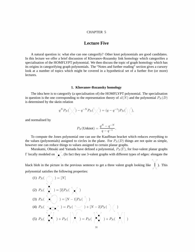
The idea here is to categorify (a specialisation of) the HOMFLYPT polynomial. The specialisationin question is the one corresponding to the representation theory ofsl(N) and the polynomialPN (D)is determined by the skein relation

qNPN ( )− q−NPN ( ) = (q − q−1)PN ( ),

and normalised by

PN (Unknot) =qN − q−N

q − q−1.

To compute the Jones polynomial one can use the Kauffman bracket which reduces everything tothe values (polynomials) assigned to circles in the plane. For PN (D) things are not quite as simple,however one can reduce things to values assigned to certain planar graphs.

Murakami, Ohtsuki and Yamada have defined a polynomial,PN (Γ), for four-valent planar graphs

Γ locally modeled on . (In fact they use 3-valent graphs with different types of edges: elongate the

black blob in the picture in the previous sentence to get a three valent graph looking like ). This

polynomial satisfies the following properties:

(1) PN ( ) = [N ]

(2) PN ( ) = [2]PN ( )

(3) PN ( ) = [N − 1]PN ( )

(4) PN ( ) = PN ( ) + [N − 2]PN ( )

(5) PN ( ) + PN ( ) = PN ( ) + PN ( )

31

32 5. LECTURE FIVE

In the above the square brackets refer to the quantum integer, i.e.

[k] =qk − q−k

q − q−1.

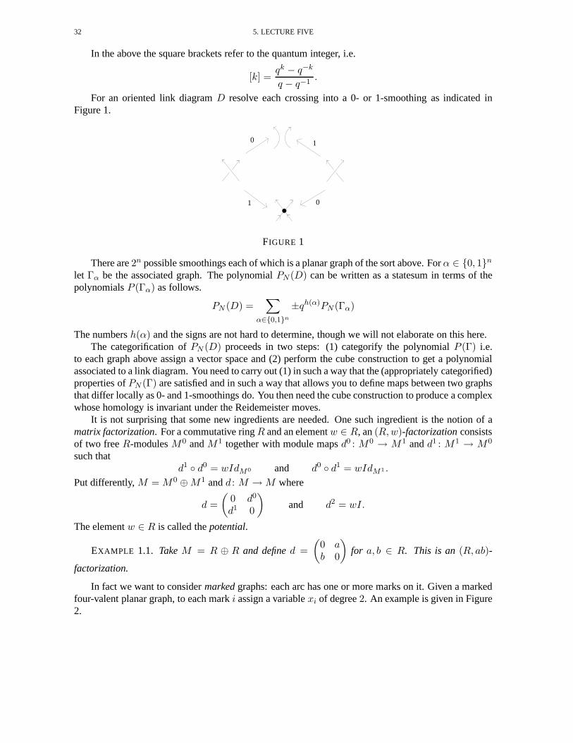
For an oriented link diagramD resolve each crossing into a 0- or 1-smoothing as indicated inFigure 1.

10

1 0

FIGURE 1

There are2n possible smoothings each of which is a planar graph of the sort above. Forα ∈ {0, 1}n

let Γα be the associated graph. The polynomialPN (D) can be written as a statesum in terms of thepolynomialsP (Γα) as follows.

PN (D) =∑

α∈{0,1}n

±qh(α)PN (Γα)

The numbersh(α) and the signs are not hard to determine, though we will not elaborate on this here.The categorification ofPN (D) proceeds in two steps: (1) categorify the polynomialP (Γ) i.e.

to each graph above assign a vector space and (2) perform the cube construction to get a polynomialassociated to a link diagram. You need to carry out (1) in sucha way that the (appropriately categorified)properties ofPN (Γ) are satisfied and in such a way that allows you to define maps between two graphsthat differ locally as 0- and 1-smoothings do. You then need the cube construction to produce a complexwhose homology is invariant under the Reidemeister moves.

It is not surprising that some new ingredients are needed. One such ingredient is the notion of amatrix factorization. For a commutative ringR and an elementw ∈ R, an(R,w)-factorizationconsistsof two freeR-modulesM0 andM1 together with module mapsd0 : M0 → M1 andd1 : M1 → M0

such thatd1 ◦ d0 = wIdM0 and d0 ◦ d1 = wIdM1 .

Put differently,M = M0 ⊕M1 andd : M →M where

d =

(

0 d0

d1 0

)

and d2 = wI.

The elementw ∈ R is called thepotential.

EXAMPLE 1.1. TakeM = R ⊕ R and defined =

(

0 ab 0

)

for a, b ∈ R. This is an(R, ab)-

factorization.

In fact we want to considermarkedgraphs: each arc has one or more marks on it. Given a markedfour-valent planar graph, to each marki assign a variablexi of degree2. An example is given in Figure2.

1. KHOVANOV-ROZANSKY HOMOLOGY 33

8

x

xx x

x x

x

x12

3

4

56

7

FIGURE 2

We now assign certain matrix factorizations to local piecesof the graph, which are later tensoredtogether to get something associated to the graph itself.

We indicate the type of local piece, the ringR and the potentialw in the table below.

Local piece R w

l

x xxx

i j

kQ[xi, xj, xk, xl] xN+1

i + xN+1j − xN+1

k − xN+1l

j

xx

iQ[xi, xj] xN+1

i − xN+1j

x i

Q[xi] 0

It is not particularly enlightening in such a short review toprovide the factorizations explicitly -please refer to the original source. All these factorizations are then tensored together (over a varietyof intermediate rings) to get a factorizationC(Γ) which, it turns out, is a factorization withR =Q[xi|i ∈ set of marks] andw = 0. In other words we have a length two complex. The homology ofthis complex isZ/2 ⊕ Z-graded, but is only non-zero in one of theZ/2-gradings. We writeH∗(Γ)for the homology in this non-zero grading (soH∗(Γ) is a gradedQ-vector space). The assignmentΓ 7→ H∗(Γ) categorifies the polynomialP (Γ).

PROPOSITION1.2.∑

i

qidim(H i(Γ)) = PN (Γ)

We can now move on to defining a link homology theory. Given an oriented link diagramD putone mark on each arc of the link and define 0- and 1-smoothings as in Figure 1. The2n smoothingsΓα

are now marked graphs which as usual we index by the vertices of the cube{0, 1}n.

34 5. LECTURE FIVE

Let Vα be an appropriately shifted version ofH∗(Γα) and set

Ci,∗(D) =⊕

α∈{0,1}n

rα=i+n+

Vα.

We need a differential and the key thing is to define the “partial” derivatives along edges of thecube. Again we will skip all the details but it is possible to define maps of factorizations as indicatedbelow.

1

ixix

xx xxxj

k l

j

k l

χ

χ

0x

If Γ0 andΓ1 are graphs that agree outside a small region in which they look like the left and rightpicture above thenχ0 andχ1 induce mapsC(Γ0)→ C(Γ1) andC(Γ1)→ C(Γ0) and hence maps

χ0 : H∗(Γ0)→ H∗(Γ1) andχ1 : H∗(Γ1)→ H∗(Γ0).

Thus, to each cube edgeζ : Γ→ Γ′ we can produce a mapdζ : H∗(Γ)→ H∗(Γ′). As before set

d =∑

ζ such thatTail(ζ)=α

sign(ζ)dζ .

Miraculously this all works and the following proposition holds.

PROPOSITION1.3. (i) H(C∗,∗(D), d) is invariant under Reidemeister moves.(ii)

∑

i,j

(−1)iqjdim(H i,j(D)) = PN (D).

Clearly there are many details to check - which is why the paper by Khovanov and Rozansky runsto over one hundred pages!

2. Graph homology

The idea of graph homology is to interpret graph polynomials, like the chromatic polynomial, Tuttepolynomial etc., as the graded Euler characteristic of a bi-graded vector space. It is much simpler todo this than it is to work with links, since there is no Reidemeister invariance to check. None-the-less,graph homology is interesting in its own right and also serves as a “toy model” revealing the same sortof phenomena that arise in link homology. For example, torsion also occurs in graph homology and ismuch more abundant and easier to get hold of than in link homology.

Let us look at the example of the chromatic polynomial. LetG be a graph with vertex set Vert(G)and edge set Edge(G). Thechromatic polynomial, P (G) ∈ Z[λ] is a polynomial which when evaluatedatλ = m ∈ Z gives the number of colourings of the vertices ofG by a palette ofm colours satisfyingthe property that adjacent vertices have different colourings.

There is a procedure to calculateP (G) as follows. Number the edges ofG by 1, . . . , n and notethat there is a one-to-one correspondence between the subsets of edges ofG and the set{0, 1}n. (Anedge ofG is labelled with 1 if is is present in the subset and 0 otherwise). Forα ∈ {0, 1}n defineGα

to be the graph with Vert(Gα) = Vert(G) and

Edge(Gα) = {ei ∈ Edge(G) | thei’th entry inα is a 1}.

Now definerα = the number of 1’s inα

2. GRAPH HOMOLOGY 35

and

kα = the number of components inGα.

A state-sum formula forP (G) is given by

P (G) =∑

α∈{0,1}n

(−1)rαλkα .

EXERCISE2.1. Stop reading here and try to categorifyP (G).

To categorifyP (G) we start with a graded algebraR. For α ∈ {0, 1}n let Rα = R⊗kα and asusual form a cube: associateRα to the vertexα. A simple example is shown in Figure 3

111

1 2

3

000

100

010

001

110

101

011

FIGURE 3

Now set

Ci,∗(G) =⊕

rα=i

Rα.

To define a differential we follow the usual procedure. For a cube edgeζ : α → α′ note thatGα′

either has the same number of components asGα or one component less (two components are fusedby the additional edge inGα′ ). Thus we definedζ : Rα → Rα′ to be multiplication inR on copiesof R corresponding to components that fuse (if such exist) and the identity elsewhere. We thus get acomplex whose homology is the graph homology ofG.

PROPOSITION2.2.∑

i,j

(−1)iqjdim(H i,j(G)) = P (G)|λ→qdim(R)

EXERCISE2.3. Would takingd = 0 for the differential work as well?

There is a long exact sequence in graph homology which categorifies the deletion-contraction re-lation. Given an edgee we can form two new graphsG − e andG/e where the first has the edgeedeleted and the second contracts it. There is a short exact sequence

0 // Ci−1,j(G/e) // Ci,j(G) // Ci,j(G− e) // 0

which gives a long exact sequence

// H i−1,j(G/e) // H i,j(G) // H i,j(G− e) // .

36 5. LECTURE FIVE

3. Notes and further reading

The first graph polynomial to be categorified was the chromatic polynomial in [Helme-GuizonRong].The dichromatic polynomial was studied in [Stosic]. Torsion in graph homology has been investigatedin [Helme-GuizonPrzytyckiRong].

The reference for Khovanov-Rozansky theory is [KhovanovRozansky1]. While this theory is con-siderably harder to compute than Khovanov’s original homology some progress has been made. In[Rasmussen3] Rasmussen describes the Khovanov-Rozansky polynomial of2-bridge knots in termsof the HOMFLYPT polynomial and signature. There is an analogue of Lee’s theory investigated byGornik in [Gornik ]. The polynomial of Murakami, Ohtsuki and Yamada is defined and its propertiesstudied in [MurakamiOhtsukiYamada ].

Khovanov and Rozansky followed up their paper with a sequel [KhovanovRozansky2] in whichthey consider the two variable HOMFLYPT polynomial. Prior to Khovanov and Rozansky’s first paperthe caseN = 3 had been treated in a somewhat different manner by Khovanov in [Khovanov5].Recently, a link with Hochschild homology has been uncovered [Przytycki ].

Link diagrams can also be drawn on surfaces and the Jones polynomial can be defined in this context. Ifthe surfaceΣ is part of the structure then the diagram represents a link inanI-bundle overΣ. Khovanovhomology in this context has been studied in [AsaedaPrzytyckiSikora]. If the surface is not really partof the structure, but rather just a carrier for the diagram (so you can add/subtract handles away fromthe diagram) then equivalence classes of diagrams are knownasvirtual links. Khovanov homology ofthese has been studied in [Manturov ] and [TuraevTurner ].

The Jones polynomial corresponds to the 2-dimensional representation ofUq(sl2) and allowing otherrepresentations leads to thecoloured Jones polynomial. A link homology theory categorifying this wasdefined in [Khovanov3].

One of the most interesting questions surrounding the subject is to uncover the geometry that lies behindKhovanov homology. A proposal for a framework unifying Khovanov-Rozansky homology and knotFloer homology has be put forward in [DunfieldGukovRasmussen].

In a different direction P. Seidel and I. Smith have constructed a homology theory for links usingsymplectic geometry [SeidelSmith]. This theory is conjectured to be isomorphic to Khovanov homol-ogy (after suitably collapsing the bi-grading into a singlegrading). Building on this Manolescu hasconstructed a similar theory for eachN and conjectured this to be isomophic to Khovanov-Rozanskyhomology [Manolescu].

Another exciting direction is to try to give some “physical”interpretation for Khovanov homology (inthe sense that Witten gave a physical interpretation of the Jones polynomial as the partition functionof a quantum field theory). S. Gukov, A. Schwartz and C. Vafa have made an attempt in this direction[GukovSchwartzVafa] conjecturing a connection to string theory.

Last, but certainly not least, there has been a huge effort towrite computer programs to calculateKhovanov homology groups. The first of these by Bar-Natan (using Mathematica) coped with links upto 11 or 12 crossings. This was improved on by Shumakovitch [ShumakovitchKhoHo] with a programusing Pari. Bar-Natan now has a nice theoretical trick whichspeeds things up considerably. This hasbeen implemented by Jeremy Green and you can download the package at from the (wonderful) knotatlas (set up by Dror Bar-Natan and Scott Morrison).

http://katlas.math.toronto.edu/wiki/

Bibliography

[Abrams] L. Abrams, Two dimensional topological quantum field theories and Frobenius algebras ,J. Knot Theory and itsRamifications5 (1996) 569-587.

[AsaedaPrzytycki] M. Asaeda and J. Przytycki, Khovanov homology: torsion and thickness, math.GT/0402402.[AsaedaPrzytyckiSikora] M. Asaeda, J. Przytycki and A. Sikora, Categorification of the Kauffman bracket skein module of

I-bundles over surfaces,Alg. Geom. Top., 4 (2004), 1177-1210.[Bar-Natan1] D. Bar-Natan, Khovanov’s homology for tangles and cobordisms,Geometry and Topology, 9 (2005), 1443-

1499.[Bar-Natan2] D. Bar-Natan, On Khovanov’s categorificationof the Jones polynomial,Alg. Geom. Top., 2 (2002), 337-370.[CarterSaito] J.S. Carter and M. Saito,Knotted surfaces and their diagrams, Mathematical Surveys and Monographs, Vol.

55, AMS 1998.[CarterSaitoSatoh] J.S. Carter, M. Saito and S. Satoh, Ribbon-moves for 2-knots with 1-handls attached and Khovanov

Jacobsson numbers, math.GT/0407493.[DunfieldGukovRasmussen] N. Dunfield, S. Gukov and J. Rasmussen, The superpolynomial for knot homologies,

math.GT/0505662.[Gornik] B. Gornik, Note on Khovanov link cohomology, math.QA/0402266.[GukovSchwartzVafa] S. Gukov, A. Schwartz and C. Vafa, Khovanov-Rozansky homology and topological strings, hep-

th/0412243.[HeddenOrding] M. Hedden and P. Ording, The Ozsvath-Szab´o and Rasmussen concordance invariants are not equal,

math.GT/0512348, 2005.[Helme-GuizonPrzytyckiRong] L. Helme-Guizon, J. Przytycki and Y. Rong, Torsion in graph homology, math.GT/0507245.[Helme-GuizonRong] L. Helme-Guizon and Y. Rong, A categorification for the chromatic polynomial,Alg. Geom. Top, Vol.

5 (2005) 1365-1388.[Jacobsson] M. Jacobsson,An invariant of link cobordisms from Khovanov homology,Alg. Geom. Top, Vol. 4 (2004) 1211-

1251.[Khovanov1] M. Khovanov, A categorification of the Jones polynomial,Duke Math J., 101 (2000), 359-426.[Khovanov2] M. Khovanov, A functor valued invariant for tangles, math.GT/0103190.[Khovanov3] M. Khovanov, Categorifications of the colored Jones polynomial, math.QA/0302060.[Khovanov4] M. Khovanov, Link homology and Frobenius extensions, math.QA/0411447.[Khovanov5] M. Khovanov,sl(3) link homology,Alg. Geom. Top, Vol. 4 (2004) 1045-1081.[KhovanovRozansky1] M. Khovanov and L. Rozansky, Matrix factorizations and link homology, math.QA/0401268.[KhovanovRozansky2] M. Khovanov and L. Rozansky, Matrix factorizations and link homology II, math.QA/0505056.[Kock] J. Kock,Frobenius Algebras and 2-D Topological Quantum Field Theories, LMS Student Texts (No. 59), Cambridge

University Press, 2003.[KronheimerMrowka] P. Kronheimer and T. Mrowka, Gauge theory for embedded surfaes, I,Topology32 (1993), 773-826.[Lee] E. Lee, An endomorphism of the Khovanov invariant, math.GT/0210213.[MackaayTurnerVaz] M. Mackaay, P. Turner and P. Vaz, A remark on Rasmussen’s invariant of knots, math.GT/0509692.[Manolescu] C. Manolescu, Link homology theories from symplectic geometry, math.SG/0601629.[Manturov] V. Manturov, The Khovanov complex for virtual links, math.GT/0501317.[MurakamiOhtsukiYamada] H. Murakami, T. Ohtsuki and S. Yamada, HOMFLY polynomial via an invariant of colored plan

graphs,Enseign. Math44 (1998), 235-360.[Przytycki] J. Przytycki, When the theories meet: Khovanovhomology as Hochschild homology of links, math.GT/0509334.[Rasmussen1] J. Rasmussen, Khovanov homology and the slicegenus, math.GT/0402131.[Rasmussen2] J. Rasmussen, Khovanov’s invariant for closed surfaces, math.GT/0502527.[Rasmussen3] J. Rasmussen, Khovanov-Rozansky homology oftwo-bridge knots and links, math.GT/0508510.[Rasmussen4] J. Rasmussen, Knot polynomials and knot homologies, math.GT/0504045[SeidelSmith] P. Seidel and I. Smith, A link invariant from the symplectic geometry of nilpotent slices, math.SG/0405089.[Shumakovitch] A. Shumakovitch, Torsion of the Khovanov homology, math.GT/0405474.[ShumakovitchKhoHo] A. Shumakovitch, KhoHo: a program forcomputing Khovanov homology,

www.geometrie.ch/KhoHo/

37

38 BIBLIOGRAPHY

[Stosic] M. Stosic, Categorification of the dichromatic polynomial for graphs, math.GT/0504239.[Tanaka] K. Tanaka, Khovanov-Jacobsson numbers and invariants of sufrace-knots derived from Bar-Natan’s theory,

math.GT/0502371.[Turaev] V. Turaev,Quantum invariants of knots and 3-manifolds, de Gruyter Studies in Mathematics, vol. 18, Walter de

Gruyter, Berlin, 1994 .[TuraevTurner] V. Turaev and P. Turner, Unoriented topological quantum field theory and link homology, math.GT/0506229.[Turner] P. Turner, Calculating Bar-Natan’s characteristic two Khovanov homology, math.GT/0411225, 2004.[Wehrli] S. Wehrli, Khovanov homology and Conway mutation,math.GT/0301312.[Viro] O. Viro, Remarks on the definition of the Khovanov homology, math.GT/0202199.