pauli frames for quantum computer architectures

Computer EngineeringMekelweg 4,

2628 CD DelftThe Netherlands

http://ce.et.tudelft.nl/

2016

MSc THESIS

Pauli Frames for Quantum ComputerArchitectures

Leon Riesebos

Abstract

Faculty of Electrical Engineering, Mathematics and Computer Science

CE-MS-2016

Quantum computers hold the promise to solve problems that are in-tractable to classical computers. Since qubits suffer from extremelyshort lifetime and unreliable operations, Quantum Error Correc-tion (QEC) forms a vital part of a quantum computer to enableFault-Tolerant quantum computing. The usage of a Pauli frame canrelax the time constraints on QEC by keeping track of detected errorsin classical logic. For the first time, in the background of a heteroge-neous quantum computer architecture, we clarified the input/outputand working principles of a Pauli frame, which can soon be mappedto a hardware implementation. We proposed the first functionalquantum computer architecture simulation platform, QPDO, whichcan connect to different quantum simulators, such as QX Simulatoror CHP, and is used to verify the logical operations of a Surface Code17 (SC17) logical qubit. Finally, by using QPDO we found that aPauli frame does not improve the Logical Error Rate (LER) of aSC17 logical qubit, which is opposite to previous understanding. Byfurther reasoning, we also expect no improvement in LER by usinga Pauli frame for surface codes with a larger distance. Neverthe-less, the usage of a Pauli frame is still crucial for relaxing the timingconstraints on QEC.


THESIS

submitted in partial fulfillment of therequirements for the degree of

MASTER OF SCIENCE

in

COMPUTER ENGINEERING

by

Leon Riesebosborn in Amsterdam, The Netherlands

Computer EngineeringDepartment of Electrical EngineeringFaculty of Electrical Engineering, Mathematics and Computer ScienceDelft University of Technology


by Leon Riesebos

Abstract

Quantum computers hold the promise to solve problems that are intractable to classical com-puters. Since qubits suffer from extremely short lifetime and unreliable operations, QuantumError Correction (QEC) forms a vital part of a quantum computer to enable Fault-Tolerantquantum computing. The usage of a Pauli frame can relax the time constraints on QEC bykeeping track of detected errors in classical logic. For the first time, in the background of a het-erogeneous quantum computer architecture, we clarified the input/output and working principlesof a Pauli frame, which can soon be mapped to a hardware implementation. We proposed thefirst functional quantum computer architecture simulation platform, QPDO, which can connectto different quantum simulators, such as QX Simulator or CHP, and is used to verify the logicaloperations of a Surface Code 17 (SC17) logical qubit. Finally, by using QPDO we found thata Pauli frame does not improve the Logical Error Rate (LER) of a SC17 logical qubit, whichis opposite to previous understanding. By further reasoning, we also expect no improvement inLER by using a Pauli frame for surface codes with a larger distance. Nevertheless, the usage ofa Pauli frame is still crucial for relaxing the timing constraints on QEC.

Laboratory : Computer EngineeringCodenumber : CE-MS-2016

Committee Members :

Advisor: Koen Bertels, CE, TU Delft

Chairperson: Koen Bertels, CE, TU Delft

Member: Carmen G. Almudever, CE, TU Delft

Member: Tim H. Taminiau, QuTech, TU Delft

Member: Leo DiCarlo, QuTech, TU Delft

Member: Xiang Fu, CE, TU Delft

i

To my parents, sister, and friends

iii

Contents

List of Figures ix

List of Tables xi

List of Acronyms xiii

Acknowledgements xv

1 Introduction 1

2 Background 3

2.1 Qubits . . . . . . . . . . . . . . . . . . . . . . . . . . . . . . . . . . . . . . 3

2.2 Quantum gates . . . . . . . . . . . . . . . . . . . . . . . . . . . . . . . . . 4

2.2.1 Single-qubit gates . . . . . . . . . . . . . . . . . . . . . . . . . . . 4

2.2.2 Multi-qubit gates . . . . . . . . . . . . . . . . . . . . . . . . . . . . 4

2.3 Quantum math formalism . . . . . . . . . . . . . . . . . . . . . . . . . . . 5

2.3.1 Group . . . . . . . . . . . . . . . . . . . . . . . . . . . . . . . . . . 5

2.3.2 Gate properties . . . . . . . . . . . . . . . . . . . . . . . . . . . . . 6

2.3.3 Gate groups . . . . . . . . . . . . . . . . . . . . . . . . . . . . . . . 6

2.4 Universal quantum computation . . . . . . . . . . . . . . . . . . . . . . . 7

2.5 Quantum error correction . . . . . . . . . . . . . . . . . . . . . . . . . . . 7

2.5.1 Surface code . . . . . . . . . . . . . . . . . . . . . . . . . . . . . . 8

2.6 Fault-tolerant quantum computing . . . . . . . . . . . . . . . . . . . . . . 10

2.6.1 Surface code 17 . . . . . . . . . . . . . . . . . . . . . . . . . . . . . 11

3 Pauli frames 15

3.1 Working principles . . . . . . . . . . . . . . . . . . . . . . . . . . . . . . . 15

3.2 System specification . . . . . . . . . . . . . . . . . . . . . . . . . . . . . . 16

3.3 Applications and benefits . . . . . . . . . . . . . . . . . . . . . . . . . . . 19

3.4 Pauli frame example . . . . . . . . . . . . . . . . . . . . . . . . . . . . . . 21

3.5 Implementation . . . . . . . . . . . . . . . . . . . . . . . . . . . . . . . . . 23

3.5.1 Quantum control unit . . . . . . . . . . . . . . . . . . . . . . . . . 24

3.5.2 Pauli frame unit . . . . . . . . . . . . . . . . . . . . . . . . . . . . 25

4 Simulation platform 29

4.1 Quantum simulators . . . . . . . . . . . . . . . . . . . . . . . . . . . . . . 31

4.1.1 QX Simulator . . . . . . . . . . . . . . . . . . . . . . . . . . . . . . 31

4.1.2 CHP . . . . . . . . . . . . . . . . . . . . . . . . . . . . . . . . . . . 31

4.2 QPDO . . . . . . . . . . . . . . . . . . . . . . . . . . . . . . . . . . . . . . 32

4.2.1 Layered structure . . . . . . . . . . . . . . . . . . . . . . . . . . . . 32

v

4.2.2 Shared data structures . . . . . . . . . . . . . . . . . . . . . . . . . 334.2.3 Implemented layers . . . . . . . . . . . . . . . . . . . . . . . . . . . 344.2.4 Test benches . . . . . . . . . . . . . . . . . . . . . . . . . . . . . . 35

5 Experiments 375.1 Ninja star logical operations verification . . . . . . . . . . . . . . . . . . . 37

5.1.1 Run-time properties of a Ninja star . . . . . . . . . . . . . . . . . . 375.1.2 Logical operation conversion and property updating . . . . . . . . 385.1.3 QPDO implementation . . . . . . . . . . . . . . . . . . . . . . . . 385.1.4 Simulation results . . . . . . . . . . . . . . . . . . . . . . . . . . . 39

5.2 Pauli frame verification . . . . . . . . . . . . . . . . . . . . . . . . . . . . 425.2.1 QPDO implementation . . . . . . . . . . . . . . . . . . . . . . . . 435.2.2 Random circuit simulation results . . . . . . . . . . . . . . . . . . 435.2.3 Ninja star measurement simulation results . . . . . . . . . . . . . . 46

5.3 Ninja star logical error rates . . . . . . . . . . . . . . . . . . . . . . . . . . 475.3.1 Test setup . . . . . . . . . . . . . . . . . . . . . . . . . . . . . . . . 485.3.2 Results . . . . . . . . . . . . . . . . . . . . . . . . . . . . . . . . . 50

6 Conclusion 63

Bibliography 67

vi

List of Figures

2.1 The layout of a surface code using 17 qubits, also known as the ninja star. 9

2.2 Left the orientation and naming of the qubits, right the circuit for theX parity checks. . . . . . . . . . . . . . . . . . . . . . . . . . . . . . . . 10

2.3 Left the orientation and naming of the qubits, right the circuit for theZ parity checks. . . . . . . . . . . . . . . . . . . . . . . . . . . . . . . . . 10

2.4 Logical Pauli operations for a ninja star. . . . . . . . . . . . . . . . . . . 12

2.5 Rotation of a ninja star. . . . . . . . . . . . . . . . . . . . . . . . . . . . 12

2.6 Execution scheme of a ninja star logical qubit. . . . . . . . . . . . . . . . 13

3.1 Representation of the location of the Pauli frame unit. . . . . . . . . . . 17

3.2 A layered system with physical qubits, a Pauli frame unit and a QuantumError Correction layer. . . . . . . . . . . . . . . . . . . . . . . . . . . . . 20

3.3 Schedules of steps in the Quantum Error Correction process with andwithout Pauli frame. . . . . . . . . . . . . . . . . . . . . . . . . . . . . . 20

3.4 The schematic overview of the data qubits of the ninja star and theircorresponding Pauli records. . . . . . . . . . . . . . . . . . . . . . . . . . 21

3.5 All data qubits and their corresponding Pauli records are reset to beable to initialize the ninja star. . . . . . . . . . . . . . . . . . . . . . . . 21

3.6 Two errors are detected and processed by the Pauli frame. . . . . . . . . 22

3.7 A double error on D4 is detected and processed by the Pauli frame. . . 22

3.8 A logical Hadamard gate is applied an the Pauli records are mapped. . . 22

3.9 All data qubits are measured and measurement results are mapped bytheir corresponding Pauli record. . . . . . . . . . . . . . . . . . . . . . . 23

3.10 Simplified quantum computer architecture for a ninja star. . . . . . . . . 24

3.11 Detailed schematic of the Pauli Frame Unit. . . . . . . . . . . . . . . . . 26

3.12 Schematics how the Pauli arbiter and Pauli Frame Unit process differentoperations. . . . . . . . . . . . . . . . . . . . . . . . . . . . . . . . . . . . 28

4.1 The global picture of a quantum computing environment. . . . . . . . . 30

4.2 Compiler infrastructure . . . . . . . . . . . . . . . . . . . . . . . . . . . 30

4.3 Schematics for QPDO control stacks with layers. . . . . . . . . . . . . . 33

4.4 A schematic view of data structure for a circuit consisting of time slotswith operations. . . . . . . . . . . . . . . . . . . . . . . . . . . . . . . . . 34

4.5 A schematic view of a control stack and a test bench. . . . . . . . . . . . 35

5.1 The test setup for simulations of the ninja star control software. . . . . . 40

5.2 Schematic overview of a control stack with a Pauli frame layer and aQxCore layer. . . . . . . . . . . . . . . . . . . . . . . . . . . . . . . . . . 44

5.3 The test setup for the random-circuit test bench. . . . . . . . . . . . . . 44

5.4 An example of a generated random circuit for 5 qubits with 20 gates. . . 45

5.5 The test setup with a ninja star layer and a Pauli frame layer. . . . . . . 46

5.6 The circuit used to create an odd Bell state. . . . . . . . . . . . . . . . . 46

vii

5.7 The resulting histograms of the odd Bell state test bench with and with-out Pauli frame. . . . . . . . . . . . . . . . . . . . . . . . . . . . . . . . . 47

5.8 The test setup used for the Logical Error Rate experiments. . . . . . . . 49

5.9 The scheme of Error Syndrome Measurement (ESM) results used forsuccessive windows. . . . . . . . . . . . . . . . . . . . . . . . . . . . . . . 49

5.10 The stabilizer circuits used to detect logical errors. . . . . . . . . . . . . 50

5.11 Physical Error Rate versus Logical Error Rate for a Surface Code 17logical qubit without Pauli frame. . . . . . . . . . . . . . . . . . . . . . . 51

5.12 Physical Error Rate versus Logical Error Rate around the pseudo-threshold for a Surface Code 17 logical qubit without Pauli frame. . . . 51

5.13 Physical Error Rate versus Logical Error Rate for a Surface Code 17logical qubit with Pauli frame. . . . . . . . . . . . . . . . . . . . . . . . . 52

5.14 Physical Error Rate versus Logical Error Rate around the pseudo-threshold for a Surface Code 17 logical qubit with Pauli frame. . . . . . 52

5.15 Physical Error Rate versus Logical Error Rate for a Surface Code 17logical qubit with (red circles) and without (blue squares) Pauli frame. . 53

5.16 Physical Error Rate versus Logical Error Rate for a Surface Code 17logical qubit with (red circles) and without (blue squares) Pauli framearound the pseudo-threshold. . . . . . . . . . . . . . . . . . . . . . . . . 53

5.17 The absolute Logical Error Rate difference between the experiments withand without Pauli frame (red triangles) plotted together with the stan-dard deviations of the LER results (vertical bars). . . . . . . . . . . . . 54

5.18 The absolute Logical Error Rate difference between the experiments withand without Pauli frame (red triangles) plotted together with the stan-dard deviations of the LER results (vertical bars) around the pseudo-threshold. . . . . . . . . . . . . . . . . . . . . . . . . . . . . . . . . . . . 55

5.19 The coefficient of variation of the number of counted windows with (redcircles) and without (blue squares) Pauli frame. . . . . . . . . . . . . . . 55

5.20 The coefficient of variation of the number of counted windows with(red circles) and without (blue squares) Pauli frame around the pseudo-threshold. . . . . . . . . . . . . . . . . . . . . . . . . . . . . . . . . . . . 56

5.21 The resulting ρ-values from the independent t-test performed on thedata sets obtained with and without Pauli frame for different PhysicalError Rate values. . . . . . . . . . . . . . . . . . . . . . . . . . . . . . . 56

5.22 The resulting ρ-values from the paired t-test performed on the data setsobtained with and without Pauli frame for different Physical Error Ratevalues. . . . . . . . . . . . . . . . . . . . . . . . . . . . . . . . . . . . . . 57

5.23 The resulting ρ-values from the independent t-test performed on thedata sets obtained with and without Pauli frame for different PhysicalError Rate values. . . . . . . . . . . . . . . . . . . . . . . . . . . . . . . 57

5.24 The resulting ρ-values from the paired t-test performed on the data setsobtained with and without Pauli frame for different Physical Error Ratevalues around the pseudo-threshold. . . . . . . . . . . . . . . . . . . . . 58

5.25 The percentage of gates and time slots saved by the Pauli frame duringLogical Error Rate simulations for X errors. . . . . . . . . . . . . . . . . 59

viii

5.26 The percentage of gates and time slots saved by the Pauli frame duringLogical Error Rate simulations for X errors around the pseudo-threshold. 59

5.27 The upper-bound on the relative improvement in Logical Error Ratethat can be obtained by using a Pauli frame for tsESM = 8. . . . . . . . 61

ix

List of Tables

2.1 Stabilizers of the Surface Code 17. . . . . . . . . . . . . . . . . . . . . . 92.2 Additional stabilizers to describe the SC17 logical states. . . . . . . . . . 92.3 List of how logical operations are implemented for Surface Code 17. . . 13

3.1 Pauli frame execution steps for different operations. . . . . . . . . . . . . 173.2 The modifications for measurement results of qubit q with Pauli record

Rq. . . . . . . . . . . . . . . . . . . . . . . . . . . . . . . . . . . . . . . . 173.3 The mappings for Pauli record Rq for the Pauli generators. . . . . . . . 183.4 The mappings for Pauli record Rq the for single qubit Clifford generators. 183.5 The mappings for the CNOT gate on Pauli records Rc and Rt for the

control and target qubits. . . . . . . . . . . . . . . . . . . . . . . . . . . 19

4.1 The functions of the shared Core interface between layers in QPDO. . . 33

5.1 List of how logical operations are performed for a ninja star. . . . . . . . 375.2 List of properties of a ninja star. . . . . . . . . . . . . . . . . . . . . . . 385.3 List of logical operations and their relation to properties of a ninja star. 395.4 List of all classes used for the implementation of a ninja star layer in

QPDO with their corresponding responsibilities. . . . . . . . . . . . . . . 405.5 Logical initial state, expected state after applying a logical CNOT gate

(with qubit 0 as control and qubit 1 as target), and the state obtainedby simulation. . . . . . . . . . . . . . . . . . . . . . . . . . . . . . . . . . 41

5.6 Logical initial state, expected state after applying a logical CZ gate, andthe state obtained by simulation. . . . . . . . . . . . . . . . . . . . . . . 42

5.7 Pauli frame execution steps for different operations. . . . . . . . . . . . . 435.8 Description of the Error Syndrome Measurement circuit used for the

logical error rate experiment. . . . . . . . . . . . . . . . . . . . . . . . . 50

xi

List of Acronyms

ESM Error Syndrome Measurement

FT Fault-Tolerant

LER Logical Error Rate

LUT Look-Up Table

PEL Physical Execution Layer

PER Physical Error Rate

PF Pauli Frame

PFU Pauli Frame Unit

QASM Quantum Assembly

QCI Quantum-Classical Interface

QCU Quantum Control Unit

QEC Quantum Error Correction

QED Quantum Error Detection

QEX Quantum Execution

QISA Quantum Instruction Set Architecture

QPDO Quantum Platform Development framewOrk

SC17 Surface Code 17

SCC Surface Code Cycle

xiii

Acknowledgements

I would like to express my very great appreciation to my Thesis advisor Dr. Koen Bertelsfor providing me the opportunity to do an MSc Thesis on the interesting topic of quantumcomputing, for the valuable advice during my work, and for the great pizza/beer/wineevenings. Also, I would like to offer my special thanks to my daily supervisor Xiang Fu.His extraordinary motivation and support has been of great importance and has beenvery much appreciated.

I would like to thank my colleagues from the Quantum Computing Team of theComputer Engineering department for their support on my work. Especially I would liketo mention Nader Khammassi for his support on the QX server, Savvas Varsamopoulosfor providing me with the decoder software, and Dan Iorga for helping me with theflexible wrapper for CHP. It has been a pleasure to work with all of you as a team, andI hope we will continue to work together for a couple more years.

I wish to thank my parents and sister for their unconditional support and continuousencouragement throughout all the years of my study. This academic, as well as personalaccomplishment, would not have been possible without them.

Finally, I would like to show my gratitude to the friends that have been standing bymy side for the last years. I have always been able to count on them during the goodtimes and the bad times.

Thank you.

Leon RiesebosDelft, The NetherlandsJune 23, 2016

xv

Introduction 1Quantum computing is an emerging technique that promises to solve problems in a rea-sonable time which are intractable by classical computers. For certain problems, quan-tum computers running specialized quantum algorithms can gain exponential speedupcompared to classical computers running equivalent classical algorithms. The speedupis caused by exploiting quantum phenomena (i.e. superposition and entanglement) forcomputational purposes using qubits. Well-known applications of quantum algorithmsare factoring large numbers using Shor’s algorithm [1] and searching large data sets usingGrover’s search algorithm [2], but applications can also be found in the field of chemistry,optimization, and quantum simulation.

Superposition refers to the fact that qubits can reside in not only a single state butalso a superposition of states. A classical bit has two exclusive states, 0 or 1, and canonly be in one state at any point in time. A qubit however has two basis states, |0〉 and|1〉, and can be in a superposition of both states represented as a linear combination of |0〉and |1〉: |ψ〉 = α |0〉+ β |1〉, where α, β ∈ C are the probability amplitudes satisfying thenormalization condition |α|2+|β|2 = 1, and |α|2 / |β|2 represent the probability of gettingthe measurement result +1/−1 (resulting state |0〉/|1〉) respectively when measuring thequbit in the basis {|0〉 , |1〉}. Note that the action of measuring the qubit will project thestate of the qubit onto one of the measurement basis states which means that a quantumstate cannot be measured directly without losing the information stored.

In classical computing, a system composed by n classical bits can only store andprocess one of the 2n possible states at a time. However, in quantum computing multiplequbits can be combined, resulting in a new state that is a superposition of all 2n possiblestates |ψ〉 = α0 |0 . . . 00〉+α1 |0 . . . 01〉+ . . .+α2n−1 |1 . . . 11〉, where αi ∈ C,

∑ |αi|2 = 1.Entanglement is a special case of such combination meaning that the combined qubitstate cannot be decomposed into separate states. When applying a (quantum) operationon those combined qubits, the operation is applied on all 2n possible states at the sametime.

Various implementations of qubits and small quantum systems already exist, andall of them share one property: qubit states are very fragile. Qubits interact with theenvironment and information stored in the qubits tends to get corrupted, which is knownas decoherence. Due to decoherence, qubits cannot reliably store information for enoughtime and quantum operations are error prone. For example, superconducting qubitsmay lose their information in tens of microseconds [3, 4]. Also, quantum operations areunreliable with error rates around 0.1% [5, 3, 4]. Quantum algorithms require qubitswith long coherence time and operations with high fidelity to perform meaningful com-putations, making existing qubits unsuitable to use directly for computational purposes.For example, factoring a 2000-bit number using Shor’s algorithm is estimated to requireerror rates below 4× 10−13 [6, Appendix M] being far below current quantum operation

1

2 CHAPTER 1. INTRODUCTION

error rates.To enable quantum computing using qubits with high error rates, Quantum Error

Correction (QEC) was introduced [7]. QEC encodes a single quantum state in a logicalqubit created from multiple physical qubits and can detect errors on physical qubits basedon error syndromes. These error syndromes are created by repeatedly executing ErrorSyndrome Measurement (ESM) circuits on the qubits. The error syndromes are decodedusing classical algorithms and make it possible to find and correct erroneous qubits inthe system. By using QEC, we can create logical qubits that have lower error ratesthan the physical qubits they were made of, making it possible to satisfy the demandsof quantum algorithms to have qubits with low error rates.

Besides from the benefits, QEC introduces overhead and new challenges. Executionof ESM circuits has to be performed in short time periods putting high demands on qubitgate and measurement times. Also, decoding of error syndromes should be executed ina very short period to prevent QEC procedures from stalling. The requirement of fasterror decoding introduces high demands on the classical algorithms and computationaldevices.

The concept of Pauli frames was introduced [8] to loosen the timing constraintson ESM circuits and decoding algorithm execution time. A Pauli frame consists ofa combination of classical memory and logic that can track the errors of qubits. Byusing a Pauli frame, qubit errors found by decoding error syndromes can be tracked inclassical electronics, making it unnecessary to apply corrections on physical qubits. ThePauli frame can loosen the timing constraints on qubit measurement times and decodingalgorithms, making it easier to implement fully functional QEC.

In this work, we investigate how to implement a Pauli frame, and we propose aPauli frame implementation as part of a quantum computer architecture targeted for aSurface Code 17 (SC17) quantum chip. We perform functional simulations of quantumcomputer architectures with integrated QEC and verify the fault-tolerant operationsof SC17 systems. We also check the control logic of our Pauli frame implementationby simulation. Finally, we study the effect of a Pauli frame on the error rate of aSC17 logical qubit. Quantum simulations are performed with the universal quantumsimulator QX Simulator [9] and the stabilizer simulator CHP [10]. For simulating thequantum computer architecture and the Pauli frames, we used the QPDO software whichis specifically developed for this work.

This report is organized as follows: Chapter 2 provides a background to introducethe reader to the concepts used throughout this report. Chapter 3 introduces the readerto the concept and working principles of Pauli frames. In this chapter, we will alsodiscuss the benefits of a Pauli frame and propose an implementation as part of a quantumcomputer architecture. In Chapter 4, we introduce the simulations software that was usedfor our experiments which include a self-developed framework for functional simulationof quantum computer architectures: QPDO. Chapter 5 discusses the experiments weperformed and the results of those experiments. These experiments include verificationof the logical operations for a SC17 logical qubit, verification of the Pauli frame workingprinciples, and experiments to observe the impact of a Pauli frame on the error rate ofa SC17 logical qubit. Finally we conclude in Chapter 6.

build 0.18

Background 2The fundamental elements of quantum computers are quantum bits, also known asqubits. Qubits can be represented as mathematical objects, but can also be realizedin a physical system, just as classical bits. Bits and qubits are related to each other,but qubits extend the features of bits. The two extending features are superposition andentanglement.

2.1 Qubits

Where classic bits can only be in a 0 or 1 state at a certain point in time, qubits can bein a superposition of both. Two basis states are defined: |0〉 and |1〉. Qubits can be in alinear combination of both states and are therefor represented like: |ψ〉 = α |0〉 + β |1〉,where α, β ∈ C are complex probability amplitudes. The sum of all probabilities withina system should always be 1, therefor: |α|2+|β|2 = 1. The state of a qubit can be treatedas a unit column vector in a two dimensional complex space C2. This vector lives in theso called Hilbert space H. The states |0〉 and |1〉 are an orthonormal basis for H, also

known as the computational basis. By defining |0〉 =[1 0

]Tand |1〉 =

[0 1

]T, we can

introduce the vector notation of a qubit state as shown in Equation (2.1). This notationis known as the Dirac bra-ket notation.

|ψ〉 = α |0〉+ β |1〉 = α

[10

]+ β

[01

]=

[αβ

]where |α|2 + |β|2 = 1 (2.1)

The probabilistic nature of qubits presents themselves when being measured. Whenmeasuring a single qubit in the computational basis, there is a probability of |α|2 tomeasure |0〉/+1 and a probability of |β|2 to measure |1〉/−1. Observing a qubit collapsesits state to one of the possible measurement outcomes and destroys the information inthe probability amplitudes. As a result, α and β are not directly observable.

For an n-qubit system, the global state is represented as a column vector with 2n = Nentries. For example, an n = 2 qubit system has N = 4 basis states and can, therefore,be fully described by four complex amplitudes. The state vector of a two-qubit systemlives in a four-dimensional Hilbert space.

The state of a quantum system |ψ〉 has a global phase δ. Every state |ψ〉 couldtherefore be written like eiδ |ψ〉. Since the global phase has no observable influence onthe measurement results, it is in general ignored.

The second feature of qubits, that extends the capabilities of classical bits, is entan-glement. Qubits can be entangled with each other, which means that the state of theentire system cannot be represented as the production of individual qubit state anymore.An example of a non-entangled state is |ψ〉 = 1√

2|00〉+ 1√

2|01〉 = |0〉⊗ 1√

2(|0〉+ |1〉). This

state can still be written as the tensor product of two individual states and is therefor

3

4 CHAPTER 2. BACKGROUND

not entangled. The state |Φ〉 = 1√2

(|00〉+ |11〉) is entangled since it can not be written

as two individual states.

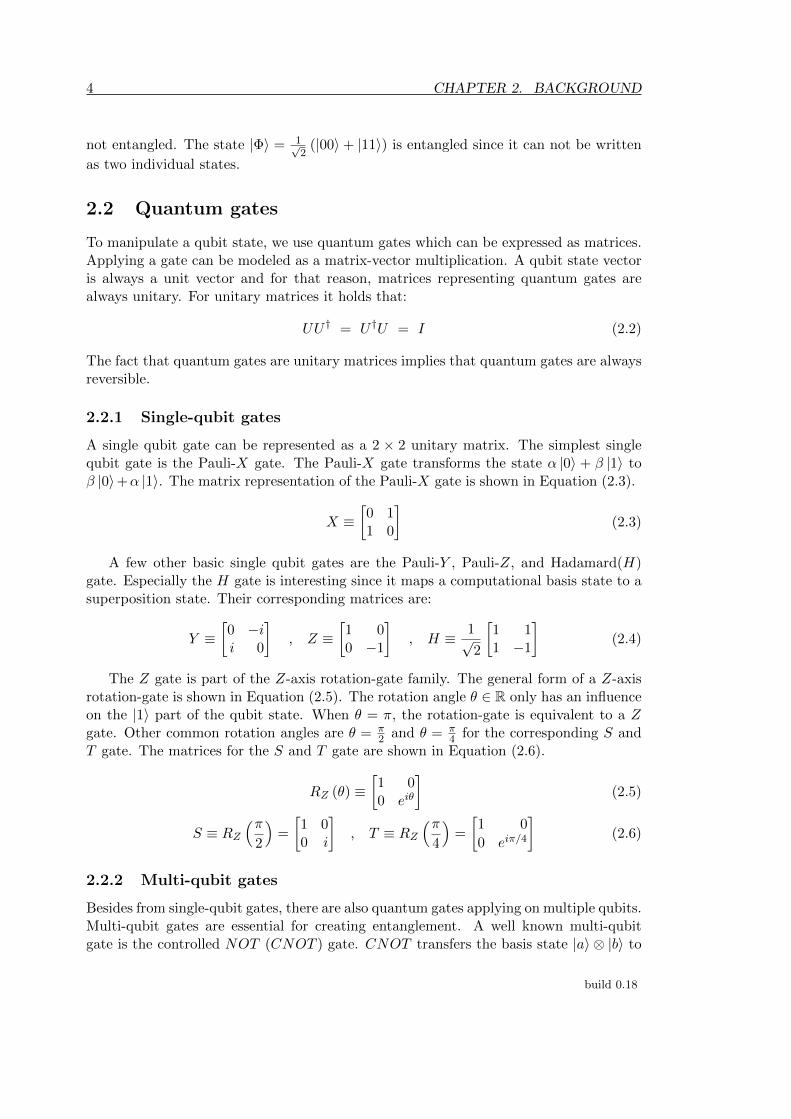
2.2 Quantum gates

To manipulate a qubit state, we use quantum gates which can be expressed as matrices.Applying a gate can be modeled as a matrix-vector multiplication. A qubit state vectoris always a unit vector and for that reason, matrices representing quantum gates arealways unitary. For unitary matrices it holds that:

UU † = U †U = I (2.2)

The fact that quantum gates are unitary matrices implies that quantum gates are alwaysreversible.

2.2.1 Single-qubit gates

A single qubit gate can be represented as a 2 × 2 unitary matrix. The simplest singlequbit gate is the Pauli-X gate. The Pauli-X gate transforms the state α |0〉 + β |1〉 toβ |0〉+α |1〉. The matrix representation of the Pauli-X gate is shown in Equation (2.3).

X ≡[0 11 0

](2.3)

A few other basic single qubit gates are the Pauli-Y , Pauli-Z, and Hadamard(H)gate. Especially the H gate is interesting since it maps a computational basis state to asuperposition state. Their corresponding matrices are:

Y ≡[0 −ii 0

], Z ≡

[1 00 −1

], H ≡ 1√

2

[1 11 −1

](2.4)

The Z gate is part of the Z-axis rotation-gate family. The general form of a Z-axisrotation-gate is shown in Equation (2.5). The rotation angle θ ∈ R only has an influenceon the |1〉 part of the qubit state. When θ = π, the rotation-gate is equivalent to a Zgate. Other common rotation angles are θ = π

2 and θ = π4 for the corresponding S and

T gate. The matrices for the S and T gate are shown in Equation (2.6).

RZ (θ) ≡[1 00 eiθ

](2.5)

S ≡ RZ(π

2

)=

[1 00 i

], T ≡ RZ

(π4

)=

[1 0

0 eiπ/4

](2.6)

2.2.2 Multi-qubit gates

Besides from single-qubit gates, there are also quantum gates applying on multiple qubits.Multi-qubit gates are essential for creating entanglement. A well known multi-qubitgate is the controlled NOT (CNOT ) gate. CNOT transfers the basis state |a〉 ⊗ |b〉 to

build 0.18

2.3. QUANTUM MATH FORMALISM 5

another basis state |a〉 ⊗ |b⊕ a〉, where a, b ∈ {0, 1} and ⊕ is classical XOR operation.The CNOT gate can also be interpreted as a controlled-X gate, which only applies an Xgate to the target qubit if the control qubit is in the |1〉 state. The matrix representingthe CNOT gate looks as follows:

UCNOT ≡

1 0 0 00 1 0 00 0 0 10 0 1 0

(2.7)

There are more two-qubit gates and among them a simple type is that with a controlqubit and a target qubit. A typical example is the controlled-Z gate, also known as theCZ gate. This gate performs a Z gate on the target qubit if the control qubit is in the|1〉 state. Three-qubit gates also exist and one commonly-used example is the Toffoligate, also known as the controlled-controlled NOT or CCNOT gate. The Toffoli gateworks similar as the CNOT gate but has two control qubits. Only if both control qubitsare in the |1〉 state, the Toffoli gate will apply a X operation to the target qubit.

2.3 Quantum math formalism

The mathematical model of quantum mechanics is mainly based on linear algebra. Inthis section, we introduce mathematical concepts which are used in the remainder of thisreport.

2.3.1 Group

As described in [11, Appendix 2], a group is defined as a 2-tuple (E, •) where E is aset and • is is the so-called group law. Groups are in general referred as E without thegroup law, but it must be defined. A subgroup F of E, noted as F ⊆ E, is a subsetof E using the same group law as E. For E to be qualified as a group, the followingrequirements must hold:

1. ∀a, b ∈ E it holds that a • b ∈ E.

2. ∀a, b, c,∈ E it holds that (a • b) • c = a • (b • c).

3. ∃e ∈ E where ∀a ∈ E it holds that e • a = a • e = a. Element e is the so calledidentity element.

4. ∀a ∈ E there ∃b ∈ E such that a • b = b • a = e.

To describe a group we can use group generators. The generators of a group S is a setGs ⊆ S such that each si ∈ S can be expressed as a finite combination of gi ∈ Gs usingthe group law of S. The set generated by Gs is 〈Gs〉 and Gs contains the generators of〈Gs〉. By describing a group by their generators, we have a compact notation that coversall the elements in a group.

A group can also have a normalizer. Assume we have a group (T, •), then thenormalizer of a group S ⊆ T is the group NS ⊆ T where ∀ni ∈ NS and ∀si ∈ S there

build 0.18


∃sj ∈ S where it holds that ni • si •n−1i = sj . This means that the normalizer of S mapselements of S to elements of S.

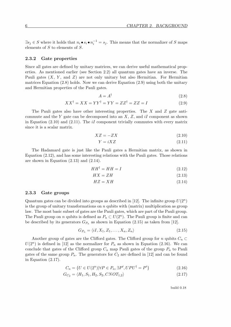
2.3.2 Gate properties

Since all gates are defined by unitary matrices, we can derive useful mathematical prop-erties. As mentioned earlier (see Section 2.2) all quantum gates have an inverse. ThePauli gates (X, Y , and Z) are not only unitary but also Hermitian. For Hermitianmatrices Equation (2.8) holds. Now we can derive Equation (2.9) using both the unitaryand Hermitian properties of the Pauli gates.

A = A† (2.8)

XX† = XX = Y Y † = Y Y = ZZ† = ZZ = I (2.9)

The Pauli gates also have other interesting properties. The X and Z gate anti-commute and the Y gate can be decomposed into an X, Z, and iI component as shownin Equation (2.10) and (2.11). The iI component trivially commutes with every matrixsince it is a scalar matrix.

XZ = −ZX (2.10)

Y = iXZ (2.11)

The Hadamard gate is just like the Pauli gates a Hermitian matrix, as shown inEquation (2.12), and has some interesting relations with the Pauli gates. Those relationsare shown in Equation (2.13) and (2.14).

HH† = HH = I (2.12)

HX = ZH (2.13)

HZ = XH (2.14)

2.3.3 Gate groups

Quantum gates can be divided into groups as described in [12]. The infinite group U(2n)is the group of unitary transformations on n qubits with (matrix) multiplication as grouplaw. The most basic subset of gates are the Pauli gates, which are part of the Pauli group.The Pauli group on n qubits is defined as Pn ⊂ U(2n). The Pauli group is finite and canbe described by its generators GPn as shown in Equation (2.15) as taken from [12].

GPn = 〈iI,X1, Z1, . . . , Xn, Zn〉 (2.15)

Another group of gates are the Clifford gates. The Clifford group for n qubits Cn ⊂U(2n) is defined in [12] as the normalizer for Pn as shown in Equation (2.16). We canconclude that gates of the Clifford group Cn map Pauli gates of the group Pn to Pauligates of the same group Pn. The generators for C2 are defined in [12] and can be foundin Equation (2.17).

Cn = {U ∈ U(2n)|∀P ∈ Pn,∃P ′, UPU † = P ′} (2.16)

GC2 = 〈H1, S1, H2, S2, CNOT1,2〉 (2.17)

build 0.18

2.4. UNIVERSAL QUANTUM COMPUTATION 7

The last group of interest is the group of non-Clifford gates. This infinite groupconsists of all the gates that are not in the Clifford group and is defined as UNC(2n) =U(2n) \ (Pn ∪ Cn) for n qubits. Concrete examples of non-Clifford gates discussed inSection 2.2 are the T gate and the Toffoli gate.

2.4 Universal quantum computation

For realizing universal quantum computation, there is a minimal set of requirementswhich includes a universal quantum gate set (as proposed in [11]). For universal quantumcomputation, the following conditions should be met:

1. Adequate amount of classical computing resources for controlling the quantumprocess.

2. Adequate amount of qubits to have a state space large enough to perform thecomputation.

3. Ability to initialize any qubit in the system to a computational basis state.

4. Ability to perform a universal set of quantum gates on any subset of qubits in thesystem.

5. Ability to perform measurements in the computational basis.

At this moment, we want to point out the definition of the universal set of quantumgates. Universal gates are a well-known concept in Boolean logic. For binary logicsystems, having NAND or NOR gates is enough to implement any arbitrary Booleanfunction. In quantum computing, a set of quantum gates is universal if any unitaryoperation can be approximated to arbitrary accuracy by a quantum circuit involving onlygates in the set. An example of a universal set of quantum gates is the set H,T,CNOT .Any universal gate set should at least contain a multi-qubit gate and a non-Clifford gate.

2.5 Quantum error correction

Up to this point, we have described qubits as mathematical objects. Just as classicalbits, qubits need to be physically realized to use them for actual calculations. Thereare many different ways to construct physical qubits, and all realizations have one factorin common: physical qubits suffer from decoherence. A qubit loses its state in a shortperiod which makes it hard to store a quantum state for a long time. Also, the physicalexecution of initialization, gates and measurement operations is not perfect and canintroduce errors.

For example, superconducting qubits may lose their information in tens of microsec-onds [3, 4] and quantum operations are unreliable with error rates around 0.1% [5, 3, 4].Quantum algorithms require qubits with long coherence time and operations with highfidelity to perform meaningful computations, making existing qubits unsuitable to usedirectly for computational purposes. For example, factoring a 2000-bit number usingShor’s algorithm is estimated to require error rates below 4 × 10−13 [6, Appendix M]

build 0.18


being far below current quantum operation error rates. To still be able to do meaningfulcomputations using qubits with high error rates, Quantum Error Correction (QEC) wasintroduced [7].

A quantum state can be encoded redundantly to protect it from noise using QECcodes. These encoding schemes entangle multiple (physical) qubits to form a logical qubitthat can store a single qubit state. By using QEC it is possible to create logical qubitsthat have lower error rates than their underlying physical qubits. These error rates arealso referred to as the Logical Error Rate (LER) and Physical Error Rate (PER). In thenext section, we will discuss a QEC scheme which is known as the surface code.

2.5.1 Surface code

The surface code is a topological QEC code [12] and is derived from Kitaev’s toric code[13]. The surface code is a promising QEC code and attracts a lot of theoretical andexperimental research [6, 12, 14, 15, 16, 17, 18, 19, 20, 21, 22]. There are several differentmethods [6, 14, 23] to encode logical qubits using the surface code. The method studiedin this thesis is to encode a logical qubit in a sheet or patch, also known as planarsurface code, and will from now on be referred to as surface code. The surface code isinteresting mainly because of its good tolerance to errors and convenient two-dimensionallayout with only nearest-neighbor qubit interactions, which contributes in a positive wayto the feasibility to manufacture such a system. The two-dimensional layout of thesurface code can exist in various shapes and sizes. Data qubits, which hold the encodedstate of the logical qubit, are aligned in a grid with ancilla qubits between them. Figure2.1 displays an example using nine data qubits (in blue) and eight ancilla qubits (inred and green). The red/green ancilla qubits are used to check X/Z parity betweenneighboring data qubits. The red and green connection lines show how ancilla qubitsinteract to the data qubits. Since the surface code checks both X and Z parity, all typesof errors can be detected. A surface code using 17 qubits, which is also known as SurfaceCode 17 (SC17) or a ninja star, can detect up to one error and is described in [19] bythe stabilizers shown in Table 2.1. The additional stabilizers that are shown in Table 2.2can be used to describe various logical states of a ninja star. More information aboutstabilizer formalism can be found in [11].

The example in Figure 2.1 shows a surface code with 17 qubits, but the surface canbe extended by repeating the two-dimensional pattern. By increasing the size of thelattice, the distance d increases where the distance is defined by [6] as the minimumnumber of gates required to inflict a logical operation (more about logical operationsin Section 2.6.1). The SC17 has a distance d = 3. The effect of a different distance dcan be explained by the threshold pth of a QEC code. The threshold pth is defined by[6] as the PER p where for p < pth, the LER PL decreases exponentially with d, whilefor p > pth, the LER PL increases with d. If we work in the regime where the PERp < pth, a larger distance d will increase the error tolerance of a QEC code and decreasethe LER. For the surface code, the threshold is defined by [6] as pth = 5.7 × 10−3. AQEC with a specified distance d also has a pseudo-threshold ppth, which is defined by[19] as the PER p where for p < ppth, the LER PL < p, while for p > ppth, PL > p. Fora certain QEC and a given distance d this means that if we work in the regime where

build 0.18

2.5. QUANTUM ERROR CORRECTION 9

PER p < pth, QEC yields logical qubits that have lower error rates than the underlyingphysical qubits.

D0 D1 D2

D3 D4 D5

D6 D7 D8

Figure 2.1: The layout of a surface code using 17 qubits, also known as the ninja star.

X Stabilizers Z Stabilizers

X0X1X3X4 Z0Z3

X1X2 Z1Z2Z4Z5

X4X5X7X8 Z3Z4Z6Z7

X6X7 Z5Z8

Table 2.1: Stabilizers of the Surface Code 17.

Stabilizer Logical state

Z0Z4Z8 |0〉L−Z0Z4Z8 |1〉LX2X4X6 |+〉L−X2X4X6 |−〉L

Table 2.2: Additional stabilizers to describe the SC17 logical states.

The surface code can detect errors by executing an error correction circuit, alsoknown as an Error Syndrome Measurement (ESM), which is performed during a SurfaceCode Cycle (SCC). When executing an ESM, all red and green ancilla qubits performa particular circuit interacting only with their neighboring data qubits. These circuitsare shown in Figure 2.2 and 2.3 and are also known as stabilizer circuits. The ancillaqubits interact with their specific neighboring data qubits at a predefined timing. Theorder of interacting with the data qubits is crucial to ensure correct functionality of theESM. Neighboring data qubits of an ancilla qubit can only be accessed in a Z or Spattern. Figure 2.2 shows the S pattern while Figure 2.3 demonstrates the Z pattern. Itis possible to use a single pattern or different patterns for red and green ancilla qubits.As shown in [19] it is preferred to use different patterns for the red and green ancilla

build 0.18


qubits to prevent error insertion in the logical state of the ninja star due to errors onancilla qubits.

b a

d c

|a〉 ⊕

|b〉 ⊕

|c〉 ⊕

|d〉 ⊕

|x〉 |0〉 H • • • • HLL✙✙✙✙✙✙ ❴❴❴❴❴❴❴❴

✤✤✤✤✤✤✤

❴ ❴ ❴ ❴ ❴ ❴ ❴ ❴

✤✤✤✤✤✤✤

Figure 2.2: Left the orientation and naming of the qubits, right the circuit for the Xparity checks.

c a

d b

|a〉 •

|b〉 •

|c〉 •

|d〉 •

|z〉 |0〉 ⊕⊕⊕⊕LL✙✙✙✙✙✙ ❴❴❴❴❴❴❴❴

✤✤✤✤✤✤✤

❴ ❴ ❴ ❴ ❴ ❴ ❴ ❴

✤✤✤✤✤✤✤

Figure 2.3: Left the orientation and naming of the qubits, right the circuit for the Zparity checks.

The execution of an ESM starts with initializing all ancilla qubits to |0〉 and applyinga Hadamard gate to the red ancilla qubits. After that, all ancilla qubits perform theirfour CNOT operations at the same time where the timing and order of the CNOToperations are crucial for correct results. After the CNOT operations, a Hadamardgate is applied on the red ancilla qubits before all ancilla qubits are measured. Themeasurement results of all ancilla qubits together form an error syndrome which can bedecoded (using a decoder) to find the most likely error happened on the data qubits. Theerror found in the data qubits can then be corrected by applying a correction gate onthe corresponding data qubit. When repeatedly executing the ESM procedure includingerror syndrome decoding and error correction, a logical state encoded in a surface codecan be protected from errors for a longer period.

2.6 Fault-tolerant quantum computing

Encoding a quantum state using a QEC code can protect it against a certain level ofnoise, but more effort is required to realize a full Fault-Tolerant (FT) quantum system.Let us first quote a definition of fault-tolerance from [11, p. 476] to make the conceptclear:

build 0.18

2.6. FAULT-TOLERANT QUANTUM COMPUTING 11

“We define the fault-tolerance of a procedure to be the property that if onlyone component in the procedure fails then the failure causes at most oneerror in each encoded block of qubits output from the procedure.”

The idea of FT quantum computing does not only require QEC but also requires usto perform operations on logical qubits without decoding the protected quantum state.Therefore, we need to have FT logical operations that operate directly on logical qubitsand prevent us from decoding an encoded state at any time. To make the concept ofFT quantum computing universal, both QEC as well as all required logical operationsfor universal quantum computing (see Section 2.4) need to be performed in a FT way.Required FT operations include initialization of logical qubits to a computational basisstate, measurement of logical qubits in the computational basis, and a universal set ofquantum gates.

2.6.1 Surface code 17

To operate the SC17 fully FT, both QEC and logical operations have to be implementedin a FT way. To make the ESM and error detection FT, we use no FT ESM and rely oncomplex decoders that can filter inconsistencies in the error syndromes. Such decodingalgorithms use d error syndromes to be able to detect errors. An example algorithm usedto decode error syndromes is the Blossom algorithm [24, 25]. SC17 supports a limitedset of FT logical operations. In the next paragraphs, we will discuss a set of FT logicaloperations and the timing challenges for the FT operation of a ninja star.

Initialization of a ninja star to the logical |0〉 state is done by executing multiplerounds of ESM and rely on the decoder to fix initialization errors. The number of errorsyndromes required for the decoder to work correctly is equal to the distance of thelogical qubit where for a SC17 logical qubit d = 3. The |0〉L state was described in [19]by the stabilizers shown in Table 2.1 and the stabilizer Z0Z4Z8. The following procedurecan be used to initialize a ninja star to the |0〉 state:

1. Reset all data qubits to the |0〉 state.

2. Execute d rounds of ESM.

3. Run regular decoding algorithms to fix initialization errors.

Logical X and Z operations are implemented by executing a chain of X or Z op-erations on the data qubits that reach from one boundary to the other boundary. Fora ninja star (as shown in Figure 2.1), the logical X gate is performed by executing Xgates on data qubit D2, D4, and D6. The logical Z gate is performed by executing Zgates on data qubit D0, D4, and D8. Figure 2.4 shows graphically how the XL and ZLoperations are performed.

The logical Hadamard gate for SC17 is implemented transversely, which means thata Hadamard gate is executed on all data qubits. After a logical Hadamard operation,the green ancilla qubits become red ancilla qubits and vice versa. The switched ancillafunctions can be interpreted as a 90 degrees rotation of the lattice. Therefore, the XL

and ZL operations also rotate with 90 degrees. Despite from the lattice rotation, the

build 0.18


X

X

X

(a) XL operation for a ninja star.

Z

Z

Z

(b) ZL operation for a ninja star.

Figure 2.4: Logical Pauli operations for a ninja star.

addressing of the qubits does not change. Figure (2.5) shows a graphical representationof the rotation and the modified logical Pauli gates.

D0 D2

D3 D5

D6 D7 D8

D1

D4

ZLXLD0 D2

D3 D5

D6 D7 D8

D1

D4

Figure 2.5: Rotation of a ninja star.

For SC17, the logical CNOT gate can be implemented by transversely applyingCNOT gates between the data qubits of two logical qubits. The transversal CNOTLoperation between two logical qubits is dependent on the rotation of the lattices. Aninja star can be in a normal orientation or a rotated orientation due to a HL opera-tion. If two ninja stars A and B share the same orientation, the transversal CNOTL isexecuted between data qubits (ADn, BDn) where n ranges from 0 to 8. In case the ninjastars are in different orientations, the transversal CNOTL is executed in a rotated fash-ion. The CNOT operations will be executed between the following pairs of data qubitsof ninja star A and B: {(AD0, BD6), (AD1, BD3), (AD2, BD0), (AD3, BD7), (AD4, BD4),(AD5, BD1), (AD6, BD8), (AD7, BD5), (AD8, BD2)}.

The logical CZ gate for planar surface code is executed transversally, just like theCNOTL. The only difference is the way to deal with different rotational orientations ofninja stars. If the orientation of two ninja stars A and B is different, the transversalCZL gate is executed between data qubits (ADn, BDn) where n ranges from 0 to 8. Incase ninja star A and B share the same orientation, the transversal CZL is executed ina rotated fashion as explained for the CNOTL.

Logical measurement of a ninja star in the ZL basis can be performed by measuringall data qubits (transversal measurement) in the Z basis. The product of the dataqubit measurement outcomes (±1) will yield the logical qubit measurement result. The

build 0.18

2.6. FAULT-TOLERANT QUANTUM COMPUTING 13

procedure for FT logical measurement can be summarized in the following steps:

1. Measure all data qubits in the computational basis. Retrieve their measurementoutcomes.

2. Run several ESM rounds, but only for the Z ancillas. Running the partial ESMenables us to detect possible X errors that happened during the measurementprocedure.

3. Calculate the product of the measurement outcomes (±1) of all data qubits. Theresult, which can be seen as a parity check, represents the logical measurementoutcome.

Table 2.3 recaps in one table how FT logical operations are implemented for SC17.

Logical operation Implementation

XL ChainZL ChainHL Transversal

CNOTL TransversalCZL Transversal

Reset to |0〉L TransversalMZL

Transversal

Table 2.3: List of how logical operations are implemented for Surface Code 17.

ESM rounds can repeatedly be executed to correct and maintain a ninja star statefor a longer period. We can execute one or more (1..*) rounds of ESM to collect enougherror syndromes for the used decoder. The decoder can generate a set of correctionswhich can then be applied on the data qubits. After applying the corrections, we canapply a logical operation before we execute the next rounds of ESM. By repeatingthis execution scheme of 1 or more rounds of ESM, decoding, applying corrections, andlogical operations we can perform FT computations with logical qubits while protectingthe logical state from errors. A schematic view of the execution scheme is shown inFigure 2.6.

Time

ESM (1..*)

Correct errors

Logical operation

Decoding time Decoding time

Figure 2.6: Execution scheme of a ninja star logical qubit.

build 0.18


build 0.18

Pauli frames 3In the previous chapter, we have seen that qubits suffer from decoherence. Execution offewer gates on qubits can result in reduced operation times, which reduces the probabilityof errors. A technique that reduces the amount of gates that have to be applied on qubitsis called Pauli frames. This chapter explains more about the technique and the benefitsof Pauli frames.

3.1 Working principles

The basic idea of Pauli frames is to track gates from the Pauli group in classical electronicsinstead of applying them on qubits. In that case, every qubit in the system has a Paulirecord that tracks the Pauli gates for that specific qubit. The Pauli records of all qubitsin a quantum system make a Pauli frame. This idea was first proposed in [8] but hasalso been discussed in [26, 27, 12, 28, 17]. Three essential elements form the basis of theworking principles of Pauli frames:

1. The first element is the effect of qubit initialization on a Pauli record. If a qubitis initialized to |0〉, its corresponding Pauli record is reset to an empty state (i.e.nothing was tracked yet). All tracked Pauli operators from the past are erased,and the system is in a known state.

2. The second element is the effect of the Pauli records on qubit measurements inthe Z basis. Assume mq is the measurement result of qubit q which was measuredin the Z basis and Rq is the Pauli record of qubit q. All tracked Pauli operatorscan be described by the generators of the Pauli group GPn as defined in equation(2.15). We can conclude that Rq can be expanded to a series of X, Z, and iI gates.Both Z and iI gates have no effect on the measurement result (see equation (3.1)).Only the X gates in Rq have an effect on the measurement result. An odd amountof X gates in Rq will invert measurement result mq to −mq (see equation (3.2))while an even amount of X gates in Rq will have no effect on mq.

mq · Z ≡ mq · iI ≡ mq (3.1)

mq ·X ≡ −mq (3.2)

3. The last element is based on the gate groups mentioned in Section 2.3.3. Letus recall the group of Clifford operators on n qubits Cn and the group of Paulioperators on n qubits Pn. For those groups it holds that Cn is the normalizer ofPn, as defined in Section 2.3.1. This means that every Clifford gate ci ∈ Cn mapsa Pauli gate pi ∈ Pn to a Pauli gate pj ∈ Pn. In short, for ∀n it holds that for

15

16 CHAPTER 3. PAULI FRAMES

∀ci ∈ Cn and ∀pi, pj ∈ Pn, cipi = pjci. Since it is know that all elements in Cnhave an inverse, it also holds that cipic

−1i = pj . This means that the application

of a Clifford gate ci on qubit q will map the corresponding Pauli record Rq to anew valid Pauli record R′q.

Up to now, we assumed that all Pauli gates have to be tracked. Fortunately, thisis not the case since Pauli gates have certain beneficial properties and global phase hasno effect on the measurement results. All Pauli gates tracked in Pauli record Rq can bedecomposed into a series of Pauli generators as described in equation (2.15). Since globalphase has no effect on measurement results, only the X and Z generators have to betracked in the Pauli records. We define R′q as the Pauli record which only contains the Xand Z elements of Rq. The Pauli generators X and Z anti-commute (i.e. XZ = −ZX).Reordering the elements of R′q can only introduce new global phase elements which againcan be dropped. In this case, we can order R′q in a way where all X gates and Z gatesare combined. Since X and Z gates are Hermitian, every even sequence of those gateswill cancel to I as described in equation (2.9). By canceling out as much as possible Xand Z gates we can compress R′q to R′′q where R′′q contains a maximum of one X gateand one Z gate. We can conclude that any Pauli record Rq can be expressed by one outof four compressed records R′′q ∈ {I,X,Z,XZ}.

Up to now, we described how Pauli frames can handle qubit initialization, qubitmeasurement, Pauli gates and Clifford gates. In Section 2.4, we defined the requirementsfor universal quantum computation. All requirements mentioned are met, except forrequirement 4: The ability to perform a universal set of quantum gates. Pauli frames arenot compatible with non-Clifford gates, and therefore, the mechanism can not support auniversal set of quantum gates. Non-Clifford gates can still be applied by flushing Paulirecord Rq of qubit q before applying the non-Clifford gate on qubit q which means thatall pending Pauli gates in record Rq are executed on qubit q to empty the record. Nowthe non-Clifford gate can be applied on qubit q. After the non-Clifford gate, Pauli gatescan be tracked again. By using this flushing technique, the Pauli frame technique canbe utilized as an architectural component of a universal quantum computer.

3.2 System specification

Every physical qubit in a quantum system will be assigned a piece of classical memory tostore the Pauli record of that qubit. The Pauli records of all qubits in a single quantumsystem together make a Pauli frame. Since every Pauli record Rq ∈ {I,X,Z,XZ}, everyPauli record can be a 2-bit memory. A system with n qubits will need 2n bits of memoryfor the Pauli frame. The Pauli frame together with required Pauli frame mapping logicwill be called a Pauli Frame Unit (PFU). A Pauli frame can be seen as an abstract layeron top of the qubits that exists in the classical domain as shown in Figure 3.1. In thisfigure, Operations′ does not have to be equal to Operations.

Different operations are handled in a variety of ways by the Pauli arbiter and the PFU.The operations can be divided into five categories: Initialization (in the computationalbasis), Measurement (in the computational basis), Pauli gates, Clifford gates, and non-Clifford gates. Table 3.1 presents how every category is processed.

build 0.18

3.2. SYSTEM SPECIFICATION 17

Qubits

Pauli Frame Unit

Qubits

Operations Operations

Operations'

Figure 3.1: Representation of the location of the Pauli frame unit.

Operations Execution steps

Initialization to |0〉 1. Initialize the target qubit to |0〉.2. Set the corresponding Pauli record to I.

Measurement 1. Measure target qubit.2. Modify measurement result based on Pauli record.

Pauli gates 1. Map Pauli record (no interaction with qubit).

Clifford gates 1. Map Pauli record(s).2. Apply Clifford gate on target qubit(s).

Non-Clifford gates 1. Flush Pauli record(s).a. Apply gates in Pauli record(s) on target qubit(s).b. Reset Pauli record(s) to I.

2. Apply non-Clifford gate on target qubit(s).

Table 3.1: Pauli frame execution steps for different operations.

From Table 3.1, we can see that measurement results are modified based on thecurrent state of the target qubit Pauli record. If the Pauli record of the measured qubitcontains an X operator (i.e. Rq ∈ {X,XZ}), the measurement result is inverted asdefined in equation (3.2). In any other case, the measurement remains in its originalstate. These modifications to the measurement results are shown in Table 3.2.

Pauli record Rq Modified measurement result

I mq

X −mq

Z mq

XZ −mq

Table 3.2: The modifications for measurement results of qubit q with Pauli record Rq.

Pauli gates modify the Pauli record of the target qubit and do not have to be executed

build 0.18


on the actual qubits. The mapping of Pauli records by Pauli gates is shown in Table 3.3where Rq is the Pauli record of qubit q and R′q is the new Pauli record for qubit q. Thistable shows the mappings for the generators of the Pauli group where operators thatonly influence global phase are excluded. Mappings of other gates in the Pauli groupcan easily be derived from Table 3.3 by expanding the Pauli gate to its set of generators.

Input record Rq Executed gate Output record R′q

I X XZ Z

X X IZ XZ

Z X XZZ I

XZ X ZZ X

Table 3.3: The mappings for Pauli record Rq for the Pauli generators.

Clifford gates map Pauli records of their target qubits to new Pauli records and alsohave to be executed on the actual qubits. The mappings of Pauli records by single qubitClifford gates is shown in Table 3.4 where Rq is the Pauli record of target qubit q andR′q is the mapped Pauli record. This table only covers the generators for the single qubitClifford gates, but can easily be extended to all single qubit Clifford gates by combiningmultiple mapping rules.

Input record Rq Executed gate Output record R′q

I H IS I

X H ZS XZ

Z H XS Z

XZ H XZS X

Table 3.4: The mappings for Pauli record Rq the for single qubit Clifford generators.

Two-qubit Clifford gates map the Pauli records of both the control and the targetqubit. The Pauli record of the target qubit has an influence on the Pauli record of thecontrol qubit and vice versa because Pauli gates can propagate to other qubits throughmulti-qubit gates. Besides from mapping the Pauli record, the Clifford gate also has tobe applied on the actual qubits. Table 3.5 shows the mapping tables of the CNOT gate,

build 0.18

3.3. APPLICATIONS AND BENEFITS 19

the only two-qubit Clifford gate in the Clifford generator set. In this table, Rc and Rtare the Pauli records for the control and target qubit.

Input records Output recordControl Rc Target Rt Control R′c Target R′t

I I I IX I XZ Z ZXZ Z XZ

X I X XX X IZ XZ XZXZ XZ Z

Z I Z IX Z XZ I ZXZ I XZ

XZ I XZ XX XZ IZ X XZXZ X Z

Table 3.5: The mappings for the CNOT gate on Pauli records Rc and Rt for the controland target qubits.

3.3 Applications and benefits

The Pauli frame technique can be applied in several ways and has multiple benefits whichmake them attractive to use in real world applications. The most interesting applicationis probably to use a Pauli frame for physical qubits in combination with Quantum ErrorCorrection (QEC) (see Section 2.5). A system structure with a QEC and a Pauli frameis shown in Figure 3.2. In such a structure, correction gates from QEC, and logicalPauli gates can be handled by the Pauli frame resulting in fewer gates being executed onthe physical qubits. We compiled a few example quantum programs provided with theScaffCC compiler [29] and found that the resulting circuits contain up to 7% Pauli gates.Since Pauli gates are tracked in classical electronics only, Pauli gates are processed fasterand with a 100% fidelity.

Using a Pauli frame as shown in Figure 3.2 has a second major benefit. Correctiongates for detected errors are always Pauli gates, which means that all of them can bestored in the Pauli frame. As a result, the QEC system does not have to wait for thedecoder to generate and apply a set of corrections before we can execute a logical gateand execute the next Error Syndrome Measurement (ESM) circuit (as shown in Figure

build 0.18


QEC Layer

Qubits

Pauli Frame Layer

Commands

Figure 3.2: A layered system with physical qubits, a Pauli frame unit and a QuantumError Correction layer.

3.3a). By eliminating this dependency, we can create a new schedule for the ESM roundsand logical gates which is shown in Figure 3.3b. The new schedule effectively removesthe time reserved for applying corrections and the waiting time for the decoder, resultingin a more time-efficient schedule. As a consequence, we can perform the same number oflogical operations and ESM rounds in less time, effectively reducing the error probabilityper logical operation. On top of that, the new schedule also loosens the timing constrainton the decoding process as well as the timing constraint on the execution speed of theESM circuit.

Time

ESM (1..*)

Correct errors

Logical operation

Decoding time Decoding time

(a) Schedule without Pauli frame.

Time

Decoding time Saved time

(b) New schedule with Pauli frame.

Figure 3.3: Schedules of steps in the Quantum Error Correction process with and withoutPauli frame.

build 0.18

3.4. PAULI FRAME EXAMPLE 21

3.4 Pauli frame example

In this section, we will discuss a few examples to give a more visual representation of thePauli frame behavior. In this example case, we assume we have 17 qubits in a SurfaceCode 17 (SC17) setup, also known as the ninja star and shown in Figure 2.1. The ninjastar has 9 data qubits and 8 ancilla qubits. The system layout is presented in Figure3.2 where the Pauli frame unit resides between the qubits and the QEC layer. For thisexample, we assume that we only have a Pauli frame for the 9 data qubits. We representthe data qubits as blue circles labeled from D0 to D8. The ancilla qubits will not beshown and are considered out of scope for this illustrative example. The Pauli recordsare represented as yellow squares labeled from D0 to D8 where the labels correspond tothe labels of their qubit. The schematic system overview is shown in Figure 3.4.

D0 D1 D2

D3 D4 D5

D6 D7 D8

D0 D1 D2

D3 D4

D6 D7 D8

D5

Ninja star Pauli Frame

Figure 3.4: The schematic overview of the data qubits of the ninja star and their corre-sponding Pauli records.

The first step is to initialize the ninja star to a logical |0〉 state. All data qubits arereset and entangled, and the Pauli records of all data qubits are reset to the I state.For this example, we assume that no errors occurred during initialization. This step isillustrated in Figure 3.5. The yellow boxes of the Pauli records now show the state ofthe records and the empty blue circles indicate that the qubits are in a correct state. Alldata qubits are now entangled and represent the logical |0〉 state.

I I I

I I

I I I

I


Figure 3.5: All data qubits and their corresponding Pauli records are reset to be able toinitialize the ninja star.

We continue to apply quantum error correction on the ninja star. Assume that twoerrors are detected, an X error on data qubit D2 and a Z error on qubit D4. Thesedetected errors are corrected, and the Pauli frame processes the corrections. The Paulirecords of data qubits D2 and D4 are mapped to their corresponding values. The dataqubits stay in an erroneous state while the Pauli frame tracks the errors. Figure 3.6

build 0.18


shows the new state of the Pauli frame while the current detected errors on the ninjastar are indicated with red circles.

X

Z

XII

I Z

I I I

I


Figure 3.6: Two errors are detected and processed by the Pauli frame.

Now assume that both an X and a Z error is detected on data qubit D4, which willbe processed by the Pauli frame. The Pauli record of data qubit D4 already containeda tracked X error. The combined XZ error maps the Pauli record to Z as shown inTable 3.3. The two X errors have canceled each other out (up to a global phase whichcan be ignored), and therefore, only the Z error has to be tracked. Figure 3.7 shows thedetection event and the mapped Pauli record of D4.

XZ

XII

I X

I I I

I


Figure 3.7: A double error on D4 is detected and processed by the Pauli frame.

Let us assume a logical Hadamard gate is applied to the ninja star. Recall that thelogical Hadamard gate is implemented by applying a Hadamard gate on all data qubitsas noted in Table 2.3. The Hadamard gate is a Clifford gate and therefore maps thePauli records, but is still applied to the data qubits. Using the mappings in Table 3.4 wecan see that the two X entries in the Pauli frame will be mapped to Z entries. Figure3.8 shows the new Pauli frame state after applying the logical Hadamard gate.

H H H

H H H

H H H

ZII

I Z

III

I


Figure 3.8: A logical Hadamard gate is applied an the Pauli records are mapped.

Finally, the logical qubit is measured, which means that all data qubit are measured,

build 0.18

3.5. IMPLEMENTATION 23

and the results are combined to retrieve the logical measurement result. The Pauli framefirst processes the measurement results of the data qubits. In this example, we only havePauli records which are in the state I or Z. Both of them have no influence on themeasurement results as we can see in Table 3.2. Therefore, all measurement results canbe further processed to obtain the logical measurement result. If any Pauli record werein the state X or XZ the corresponding measurement results would have to be invertedbefore further processing.

M M M

M M M

M M M

ZII

I Z

III

I

Ninja star Pauli Frame I m0 → m0

I m1 → m1

Z m2 → m2

I m3 → m3

Z m4 → m4

I m5 → m5

I m6 → m6

I m7 → m7

I m8 → m8

Figure 3.9: All data qubits are measured and measurement results are mapped by theircorresponding Pauli record.

3.5 Implementation

Up to now, multiple papers [8, 26, 27, 12, 28, 17] have covered the topic of Pauli frames,and other papers [30, 31, 32, 33] have discussed various architectures for quantum soft-ware and hardware, but no practical implementations of Pauli frames for future quantumcomputers have been proposed so far. In this section, we would like to cover the imple-mentation of a Pauli frame in a quantum computer architecture.

In [34] we propose a heterogeneous quantum computer architecture which supportsall operations of a ninja star implemented with transmon qubits. Figure 3.10 shows asimplified version of the proposed architecture which mainly focuses on the QuantumControl Unit (QCU). The QCU decodes the instructions belonging to the QuantumInstruction Set Architecture (QISA) and performs the required quantum operations,feedback control, and QEC. The QCU can also communicate with the host CPU whereclassical computations are performed, and quantum instructions are fetched. The QCUoutputs a sequence of physical operations to the Physical Execution Layer (PEL) tocontrol the physical qubits. The PEL takes charge of all technology-dependent controlmaking the QCU technology-independent. The QCU defined in this paper can supportnot only transmon qubit but can also support other technologies.

The PEL converts the physical operations to a set of waveforms that represent ele-mentary quantum gates supported by the underlying technology. After conversion, thePEL manages the timing of the waveform outputs. These waveforms are fed to theQuantum-Classical Interface (QCI) that routes the waveforms to the correct qubits on aquantum chip. Regarding physical measurements, the PEL provides a readout pulse tothe QCI and the QCI returns the measurement signal. The PEL processes the measure-ment signal and discriminates the measurement results. These physical measurement

build 0.18


results are then returned to the QCU for further processing. In the next sections, wewill focus on the QCU and briefly discuss the main parts of this module. For moredetails about the proposed architecture, we refer to the original paper [34]. After thisbrief overview, we will focus on the PFU.

Figure 3.10: Simplified quantum computer architecture for a ninja star.

3.5.1 Quantum control unit

We assume that a binary is loaded into memory, and the instruction fetch unit fetchesthe instructions. Based on the opcode of the instruction, the arbiter sends the instruc-tion either to the host CPU or the QCU. In the remainder of the text, we focus on thearchitectural support for the execution of quantum instructions and not on the execu-tion of instructions on the classical CPU. In an earlier stage, a compiler maps a quantumcircuit using logical and virtual qubit addresses for the logical and physical qubits respec-tively. Instructions from the Quantum Instruction Cache are first address-translated bythe Q-Address Translation module which means that compiler-generated, virtual qubitaddresses are translated into physical ones. The translation procedure is based on theinformation contained in the Q Symbol Table which provides the overview of the exactphysical location of the logical qubits and contains information on what logical qubitsare still alive.

The Execution Controller can be seen as the brain of the QCU. The ExecutionController decodes the various instructions that are fetched:

• Physical gate/measurement/reset: The Execution Controller sends these in-structions to the Pauli Arbiter for further processing.

build 0.18


• Update Q Symbol Table: Based on a series of instructions such as the onesperforming a logical Hadamard gate or a logical measurement, the Q Symbol Tableneeds to be updated. Also for deallocating qubits such an update is required.

• QEC slot. The Execution Controller sends this instruction to the QEC CycleGenerator, which is triggered to generate an ESM circuit.

As far as error correction is concerned, the necessary ESM instructions for the entirequbit plane are added at run-time by the QEC Cycle Generator, based on the informationstored in the Q Symbol Table. The responsibility of the Quantum Error Detection (QED)Unit is to detect errors based on ESM results. The decoder will use decoding algorithmssuch as the Blossom algorithm [24, 25]. QED only starts to work when d rounds of errorsyndromes are collected, where d equals the distance of the surface code.

The function of the Logic Measurement Unit is to combine the data qubit measure-ment results into a logical measurement result for a logical qubit. Once the ExecutionController receives a logical measurement instruction on a specified logical qubit, it no-tifies the Logic Measurement Unit to wait for measurement results to arrive from thePEL.

3.5.2 Pauli frame unit

The Pauli Frame Unit (PFU) consists of a Pauli frame (PF data) and Pauli framemapping logic (PF logic), and works closely together with the Pauli arbiter. Figure 3.11shows a detailed schematic of the components in the PFU. The Pauli frame containsa two-bit Pauli record for every physical qubit in the system as mentioned in Section3.2. For a single SC17 logical qubit this would be 2 · 17 = 34 bit of memory. Themapping of the Pauli records based on the applied physical operations are managed bythe PF logic module which holds all the required mapping tables. Finally, the Pauliarbiter decides which operations in the stream are forwarded to the Physical ExecutionLayer (PEL) and which ones not. The proposed PFU design complies with the systemdescribed in Section 3.2 and supports all operation types mentioned in Table 3.1. In thenext paragraphs, we will explain how the different type of operations from Table 3.1 arehandled by the PFU and the Pauli arbiter.

If the Pauli arbiter receives a reset operation (step 1), the operation will be forwardedto both the PFU and the PEL (step 2). While the PEL further processes the resetoperation, the PFU also processes the reset operation using the PF logic module. ThePauli record of the target qubit will be set to I regardless of its current state (step 3).This sequence of steps is schematically shown in Figure 3.12a.

In case the Pauli arbiter receives a measurement operation (step 1), the Pauli ar-biter will forward the operation to the PEL without taking any further action (step2). The PEL and other parts of the system perform the measurement operation, andthe measurement results are returned to the QCU (step 3). This measurement result ispicked up by the PFU which maps the measurement result based on the Pauli record ofthe target qubit (step 4) using the PF logic module. Finally, the mapped measurementresult is forwarded to other parts of the QCU (step 5). The measurement procedure isschematically shown in Figure 3.12b.

build 0.18


Pauli Frame Unit

PF data

Pauli record 0

Pauli record 1

...

Pauli record n

PF logic

Pauli arbiter

Physica l E

xecu tion La yer

Operations

Measurementresults

Figure 3.11: Detailed schematic of the Pauli Frame Unit.

Pauli operations are handled in the most efficient way. When the Pauli arbiterreceives a Pauli gate (step 1), the Pauli arbiter will only forward the gate to the PFU(step 2). The PEL is not required when executing Pauli operations. The PF logic moduleof the PFU will map the Pauli record of the target qubit (step 3), and the execution ofthe Pauli gate is finished. This procedure is also shown in Figure 3.12c.

If the Pauli arbiter receives a Clifford gate (step 1), the Pauli arbiter will forwardthe gate to the PEL and the PFU (step 2). While the PEL handles further execution ofthe Clifford gate, the PF logic module of the PFU updates the Pauli record of the targetqubit(s) (step 3). Figure 3.12d shows a graphical representation of this procedure.

In case the Pauli arbiter receives a non-Clifford gate (step 1), the Pauli arbiter stallsthe stream of operations and requests the PFU to flush the Pauli record of the targetqubit (step 2). The PF logic module of the PFU returns the Pauli gate(s) currentlypresent in the Pauli record of the target qubit and resets the Pauli record to I (step 3and 4). Finally the Pauli arbiter forwards the flushed Pauli gates to the PEL and appendsthe initial non-Clifford gate (step 5 and 6). The Pauli arbiter will continue processing thestream of operations. Figure 3.12e shows the steps of handling a non-Clifford operationin a graphical way.

build 0.18


Pauli Frame Unit

PF data

PF logic

Pauli arbiter1. Reset

operation on qubit x

2. Reset operation

2. Reset operation

3. Pauli record xset to “I”

(a) Reset operation.

Pauli Frame Unit

PF data

PF logic

Pauli arbiter1. Measurement operation on qubit x

2. Measurement operation

5. Mapped measurement result

4. Map measurement result using

Pauli record x

3. Measurement result

(b) Measurement operation.

Pauli Frame Unit

PF data

PF logic

Pauli arbiter1. Pauli gate on qubit x

2. Pauli gate

3. Map Pauli record x

(c) Pauli gate.

build 0.18


Pauli Frame Unit

PF data

PF logic

Pauli arbiter1. Clifford gate on qubit x 2. Clifford gate

2. Clifford gate

3. Map Pauli record x

(d) Clifford gate.

Pauli Frame Unit

PF data

PF logic

Pauli arbiter1. Non-Clifford gate on qubit x

5. Pauli gate6. Non-Clifford gate

2. Non-Clifford gate

3. Flush Pauli record x

4. Flushed Pauli gate

(e) Non-Clifford gate.

Figure 3.12: Schematics how the Pauli arbiter and Pauli Frame Unit process differentoperations.

build 0.18

Simulation platform 4To gain more knowledge about quantum computer architectures and Pauli frames werequire a simulation platform. This simulation platform should fit into the big pictureof a full quantum computer development environment that connects from quantum al-gorithms down to the physical operations on qubits of a quantum chip.

A quantum computer will always consist of both quantum and conventional com-puting components because of the following two reasons: the quantum algorithms andconsequently the quantum applications that will be executed, include both classical aswell as quantum parts and will thus be executed by their respective computing blocks[11]. The second reason is that, as is explained in Section 2.5, a quantum computerrequires very close monitoring and, if necessary, correction by classical logic. In [34]we present a high-level view of the quantum system stack consisting of multiple layerswhich are shown in Figure 4.1. The top layers represent the algorithms for which specificlanguage constructs and compilers need to be developed such that the algorithms canexploit the underlying quantum hardware. Here the qubits are defined as logical qubits.Figure 4.2 depicts the compiler infrastructure consisting of a conventional host compilerand a quantum accelerator compiler. The former compiles the classical logic and thelatter will produce the quantum circuits. The quantum compiler will perform quantumgate decomposition, reversible circuit design, and circuit mapping but also translatesthe logical quantum operations to a series of physical operations. As represented by thethird dimension of Figure 4.1, the logical-to-physical quantum instruction translation isdriven by choices regarding the Quantum Error Correction (QEC) code for the logicalqubits.

The next layer is the Quantum Instruction Set Architecture (QISA) which is the di-viding line between hardware and software. The algorithm designer and programmer areoffered a logical instruction set with the possibility to opt for certain encoding schemes,thus exposing the relevant error correction functionality. As stated above, the compilerwill translate logical instructions into the physical instructions that belong to the QISAand for which architectural support is provided. Examples of physical instructions inthe QISA are initialization, measurements, and quantum gates such as Hadamard andCNOT .

The Quantum Execution (QEX) block will execute the quantum instructions thatare generated by the compiler infrastructure. It will also provide the necessary hardwaresupport such as the insertion of quantum error correction circuits or the use of PauliFrames for error tracking. These operations are finally sent to the Quantum-ClassicalInterface (QCI), which will apply the proper electrical signals to the quantum chip. Notethat the QCI is responsible for all the conversions between the analog qubit plane andthe digital layers in the system stack. The QEC layer, is in charge of the error detectionand correction. It will receive the error syndrome data from the QCI which it will process

29

30 CHAPTER 4. SIMULATION PLATFORM

to identify possible errors. Then, it will make the required corrections by updating thePauli frame or by sending the appropriate corrective operations when required. TheQuantum Control Unit (QCU) proposed in Section 3.5 matches the QEX/QEC layer.

Q Algorithm

Programming Paradigm & Languages

Runtime Compiler

Q Instruction Set Architecture

QEX QEC

Quantum-Classical Interface

Q Arithmetic

Quantum Chip

Figure 4.1: The global picture of a quantum computing environment.

Figure 4.2: Compiler infrastructure

build 0.18

4.1. QUANTUM SIMULATORS 31

The main interest of this thesis lies in the QEX/QEC layer shown in Figure 4.1.The QEX/QEC layer is where the quantum computer architecture resides and where allquantum instructions are processed. The quantum algorithm and compiler levels are outof the scope of this thesis and are therefore not further discussed. This chapter presentsthe simulation software platform for the quantum layer and the QEX/QEC layer. Thesimulation platform consists of three software tools of which two are quantum simulators,and one is a self-developed software package for functional testing of quantum computerarchitectures (QPDO). These three software tools will be discussed in the remainder ofthis chapter.

4.1 Quantum simulators

Quantum behavior can be simulated on classical computers using software. There aredifferent ways to simulate qubits, and every type of simulation has its advantages anddisadvantages. In this section, we will discuss two quantum simulators which are usedfor this thesis: QX Simulator and CHP.

4.1.1 QX Simulator

The QX Simulator [9] is a universal quantum simulator developed by the Computer En-gineering lab of the Delft University of Technology. Universal quantum simulators storethe complex amplitudes of the quantum state vector. Quantum gates are represented asmatrices, and matrix-vector multiplications are used to apply gates. A universal quan-tum simulator can simulate any quantum gate by using its matrix representation, butthere are also limitations. The memory usage of universal quantum simulators grows ex-ponentially with the number of qubits simulated. Due to high memory usage, universalquantum simulators are only able to simulate up to 30 to 45 qubits depending on theavailable hardware resources.

There are two options to interface with the QX Simulator. One of them is by usingQuantum Assembly (QASM) files. These files describe quantum circuits as a list ofinstructions and are limited to quantum instructions only. The QX Simulator can readthe QASM file and execute the described circuit. The second way of interfacing withthe QX Simulator is by using sockets. The QX Simulator can start as a server andestablish TCP connections. Any program can connect to the QX server and send QASMinstructions to the QX server. The TCP connection provides a flexible and interactiveinterface to the capabilities of the QX Simulator that can be accessed from almost anydevelopment environment. The QASM syntax for both interfaces is identical.

4.1.2 CHP

The CHP quantum simulator [10] is a quantum simulator developed by Scott Aaronsonand Daniel Gottesman. CHP is a stabilizer simulator and is therefore only able to processstabilizer circuits using CNOT , H, and S gates beside from qubit initialization andmeasurement. Stabilizer simulators store a quantum state by storing the stabilizers ofthat specific state, which is very memory efficient. The limitation of stabilizer simulators

build 0.18


is that stabilizer circuits do not possess quantum speed-up regarding computation power.Stabilizer simulators are still interesting to simulate large numbers of qubits and quantumerror correction codes. CHP can read QASM like files and execute the circuit describedin the file.

For this thesis, the quantum simulation capabilities of CHP have been exposed toPython by creating a Python wrapper [35]. The Python wrapper was created using thewrapper generation software SWIG which stands for ’Simplified Wrapper and InterfaceGenerator’. CHP functionality that was exposed to Python includes the creation of aqubit register, qubit initialization, execution of quantum gates, and qubit measurements.

4.2 QPDO

For this thesis, we require a software tool that can simulate different modules of a quan-tum computer architecture in a flexible way. To enable fast development and testing, weallow functional simulation of the modules. The chosen programming language shouldbe accessible to a large crowd, cross-platform and high-level to decrease developmenttime. It is also preferable to be able to link the selected programming language easilyagainst code written in other languages. Execution speed of the quantum computerarchitecture simulations is not a constraint since we allow functional simulation. There-fore, we do not require high-speed, low-level programming languages. The tool shouldbe able to connect to different quantum simulators in a transparent way to allow sim-ulations against different simulator back-ends. The first prototypes of such a tool werewritten in Java. We experimented with different structures and design methodologiesusing the Java software. Finally, we chose to develop a tool based on a layered struc-ture programmed in Python 3. The name of the software package is Quantum PlatformDevelopment framewOrk, or in short QPDO.

4.2.1 Layered structure

QPDO provides shared interfaces and data structures to support layered systems. In-terfaces are implemented using abstract base classes and shared data structures areexpressed using classes. The layers are inspired by the OSI-model [36] and can be seenas a black box that processes a stream of commands. Every layer has its responsibilitiesand should be able to work without knowledge of lower or top layers. Commands areimplemented using function calls, and data is transferred using shared memory. Layerscan be stacked on each other in a flexible way to create a control stack. Such a controlstack contains the modules of a quantum computer architecture and enables simulationof this architecture. The bottom layer of a control stack should always be a core. Acore connects to a quantum simulator to allow simulation of the invoked commands. Acontrol stack has one core and zero or more layers on top of it. The schematic view of alayered control stack is shown in Figure 4.3a.

The key feature of the layers used in QPDO is that they all support the same interfaceand that they share the same data structures. The shared Core interface consists of aset of functions that can control quantum simulators or devices on an abstract level.The Core interface has functions for creating and removing qubits, queuing quantum

build 0.18

http://swig.org/

4.2. QPDO 33

Layer B

Layer A

Simulation Back-end

Core

Commands

(a) A schematic view of a layered controlstack in QPDO.

Layer

Simulation Back-end

Core

(b) Interfaces for the core and the other lay-ers.

Figure 4.3: Schematics for QPDO control stacks with layers.

circuits and executing queued quantum circuits. It is also possible to request the binarystate or quantum state of the system. The functions of the Core interface are listed inTable 4.1. The lowest layer in a control stack, the core, supports the functions of theshared Core interface and simulates the quantum behavior using a simulation back-end.Layers on top of the core support the shared interface too and also require a lower layerthat supports the same interface. A schematic view of a layer and core are shown inFigure 4.3b. By using this layered structure, it is possible to interchange layers easilywhich make it possible to assemble different control stacks and use different simulationback-ends.

Function Short description

createqubit(size) Allocate new qubits.removequbit() Remove existing qubits.add(circuit) Queue a quantum circuit.execute() Execute the queued quantum circuits.getstate() Retrieve the (binary) state of the qubits.

getquantumstate() Retrieve the quantum state (if supported).

Table 4.1: The functions of the shared Core interface between layers in QPDO.

4.2.2 Shared data structures

The shared data structures provided by QPDO are used to transfer information betweenlayers and to process data generated by the control stack. All shared data structuresby default provide rich functionality to analyze and manipulate its contents. The mostimportant shared data structures are the Circuit, the State, and the QuantumState. The

build 0.18


Circuit class represents a quantum circuit and contains a set of operations. Operationscan be single- or multi-qubit gates, initialization, and measurement. Operations in cir-cuits are grouped into time slots. In one time slot, every qubit can only be involved inone operation. Thereby we can see a time slot as a part of a circuit that can be executedin parallel whereby we assume that every operation takes the same amount of time toexecute. A schematic view of a circuit with time slots and operations is shown in Figure4.4.

Circuit

Time slot 0

Operation 0

Operation 1

Operation 2

Time slot 1

Operation 3

Operation 4

Time slot 2

Operation 5

Operation 6

Operation 7

Figure 4.4: A schematic view of data structure for a circuit consisting of time slots withoperations.

The State and QuantumState classes are shared data structures that describe thecurrent state of the quantum system. The State class represents a set of values thatcorrespond to the binary values of qubits. A measured qubit can either be in the 0 or 1state. A qubit that is reset to |0〉 will also be in the 0 state. After applying a quantumgate on a qubit, the state will become x (i.e. unknown) until it is measured or reset. AState object holds a set of these binary values. A QuantumState represents the full statevector with complex amplitudes and corresponding states. The QuantumState can onlybe retrieved if a simulation back-end is used that supports outputting a quantum state.

4.2.3 Implemented layers

To use QPDO for our simulations, we implemented different layers. The first imple-mented layers are two core layers that implement the Core interface: ChpCore andQxCore. The ChpCore uses the Python wrapper for CHP to use it as a simulation back-end. The CHP simulator is not universal, but can simulate Clifford gates efficiently.Since QEC codes use Clifford gates only, those can be simulated using the ChpCore.The QxCore uses the universal QX Simulator as a back-end and can simulate both Clif-ford and non-Clifford gates. The QxCore maintains a TCP connection to the QX server.Commands are sent over TCP and results are retrieved over the same connection.

Two QEC layers have been implemented: The SteaneLayer and the NinjastarLayerfor respectively the Steane code and planar surface code using 17 physical qubits perlogical qubit. The QEC layers supports generic control of independent logical qubitsincluding insertion of QEC routines, logical operation translation to a set of physicaloperations, and logical operation post-processing. As specified by QPDO, the QEClayers work in a transparent way and support the Core interface as shown in Table 4.1.

build 0.18

4.2. QPDO 35

It is for example possible to concatenate QEC layers by adding multiple QEC layers toa control stack.

To be able to test QEC layers we need to be able to insert errors. Up to now, onlyone error layer is developed, which is based on the symmetric depolarizing error model[11, 19].

In the interest of this thesis, we developed a Pauli frame layer. This layer implementsthe functionality of a Pauli frame unit as presented in Section 3.5.2. The layer managesmemory for a Pauli frame, maps the Pauli records according to mapping tables, mapsmeasurement results based on stored Pauli records, and filters Pauli gates. Since thePauli frame unit is implemented as a layer, it is possible to add multiple Pauli framelayers on different levels in a control stack.

Finally, we implemented some diagnostic layers that do not modify the commandstreams in a control stack but retrieves statistics about the command stream instead.An example of such a layer is the counter layer that counts the number of operations andcommands that pass between two other layers. The information gained by diagnosticlayers can give us useful insight into the execution flow in a control stack.

4.2.4 Test benches

The previous sections presented how control stacks can be created and configured usingQPDO. Such a control stack can potentially perform functional simulations of a quantumcomputer architecture, but requires useful input for simulation. It is possible to writecustom test benches in Python that provides input commands to a control stack anddiagnoses the output. To speed up development of test benches, QPDO provides a testbench environment and simple ready-to-use test benches.

The test bench environment provides a set of base classes that implement genericcontrol of a certain class of test benches. Generic control can contain for example loopingof a test for a certain amount of times, handling test outcomes, and acting on test results.Programmers only have to write an initialization procedure for the test bench, a singletest procedure, and a shutdown procedure for the test bench. The test bench environmentmakes it possible to develop quickly test benches that can test against various controlstacks using the generic Core interface. An example of a setup with a control stack anda test bench is shown in Figure 4.5.

Simulation Back-end

Control Stack

Test Bench

Figure 4.5: A schematic view of a control stack and a test bench.

QPDO provides a set of ready-to-use test benches that are derived from the testbench base classes. These simple test benches only need a control stack and maybe acouple of settings to run and can be used to verify the basic behavior of a control stack.

build 0.18


Two examples of such test benches are the BellStateHistoTb and the GateSupportTb.The BellStateHistoTb resets two qubits and creates a Bell state using a Hadamard anda CNOT gate. The two qubits are measured, and the results are stored. At the end ofthe test a histogram of the measurement results are printed. The GateSupportTb runsa predetermined script that tests various gates that are available in QPDO on a controlstack. It verifies if the control stack supports various gates and if the measurement resultafter the execution of the gates matches the expected outcome. Finally, the test benchprints a report that shows which gates are supported and executed correctly.

build 0.18

Experiments 5In this chapter, we present the results of the experiments performed using the simulationtools presented in Chapter 4. Three different experiments were performed consideringSurface Code 17 (SC17) and Pauli frames. The first experiment is a verification of theknown logical operations of the SC17. The second experiment is a verification of thePauli frame mechanism. With the last experiment, we investigate the impact of a Pauliframe on the error rates of a ninja star.

5.1 Ninja star logical operations verification

The first experiment is to verify the logical operations for a ninja star using QPDO. Thelogical operations we would like to verify are the initialization to |0〉, X gate, Z gate, Hgate, CNOT gate, CZ gate, and measurement in the computational basis as shown inTable 5.1.

Logical operation Implementation

XL ChainZL ChainHL Transversal

CNOTL TransversalCZL Transversal

Reset to |0〉L TransversalMZL

Transversal

Table 5.1: List of how logical operations are performed for a ninja star.

To perform the experiments to verify the ninja star logical operations, we requirespecifying which run-time properties have to be tracked for every ninja star and how wecan perform the logical operations in a correct way based on these properties. The nexttwo sections will discuss what run-time properties need to be tracked for a ninja starand how these properties cooperate with the logical operations.

5.1.1 Run-time properties of a Ninja star

To operate a Ninja star we need to track different properties which can change afterexecuting various logical operations. The first property to track is the rotation of thelattice. The rotation property of a ninja star can have two values, normal or rotated,where the rotated value indicates that the lattice is in a 90 degree rotated orientation.Tracking of the current rotation is essential for executing the correct Error Syndrome

37

38 CHAPTER 5. EXPERIMENTS

Measurement (ESM) circuit and is also required for applying logical gates in the correctway.

The second property that is tracked is the dance mode. The dance mode indicateswhenever a full ESM circuit has to be executed or if only Z ancilla qubits are active inthe ESM circuit. The dancemode property can have two values: all or z only. The valueall indicates that the full ESM circuit will be executed, while the z only value indicatesthat only Z ancilla qubits are active in the ESM circuit.

Finally, there is a state value that indicates what the current binary state is of thelogical qubit. This value can be 0, 1, or x (i.e. unknown). Table 5.2 summarizes thelist of properties for a ninja star, their possible values and the initial values at systemstart-up.

Ninja star property Possible values Initial value

rotation normal, rotated normaldancemode all, z only z only

state 0, 1, x x

Table 5.2: List of properties of a ninja star.

5.1.2 Logical operation conversion and property updating

Logical operations for ninja star logical qubits have to be converted to a set of physicaloperations and some classical post-processing. Conversion of the logical operations toa set of physical operations can be done at run-time based on the current propertiesof the involved logical qubits. Both the conversion of XL and ZL gates depend on thelattice rotation, while the conversion of transversal CNOTL and CZL gates rely on therotations of both the target and the control ninja star. The details of logical operationconversions for a ninja star are described in section 2.5.1.

Some logical operations update the run-time properties of a ninja star and thereforetheir execution requires post-processing. The HL gate inverts the current rotation of thelattice. The reset operation sets the current rotation of the ninja star to normal and thedance mode to all. Measurement requires the most post-processing. After measuringall the data qubits, the dance mode will be set to z only. Only measuring Z ancillaqubits enables us to perform partial ESM rounds that can be used to detect X errorsthat happened during the measurement of the physical qubits. If any X errors aredetected, the corresponding measurement results are corrected. Finally, the parity ofthe data qubit measurement results is calculated yielding the logical measurement resultwhich is stored in the state property of the ninja star. The relations between the logicaloperations and the properties of the logical qubit(s) they apply on are shown in Table5.3.

5.1.3 QPDO implementation

We used QPDO to verify the logical operations of the ninja star. To do so, we im-plemented a ninja star layer that accepts logical circuits as input and outputs all the

build 0.18

5.1. NINJA STAR LOGICAL OPERATIONS VERIFICATION 39

Logical operation Property dependencies Property influences

XL rotation stateZL rotation stateHL - rotation, state

CNOTL rotations stateCZL rotations state

Reset to |0〉L - rotation, dancemode, stateMZL

- dancemode, state

Table 5.3: List of logical operations and their relation to properties of a ninja star.

circuits and commands required to perform both Quantum Error Correction (QEC) andconverted logical operations. The output operations of the ninja star layer can then beexecuted on a simulation core or can be forwarded to another layer within the QPDOenvironment (see section 4.2.1). The ninja star layer can control multiple independentninja stars and also supports two-qubit logical gates. Every ninja star can have a uniqueset of ancilla qubits, or one set of ancilla qubits can be shared over all ninja stars in thesystem to lower the amount of qubits that is required to be simulated.

The ninja star layer uses multiple classes to manage all the run-time properties,execution of QEC, and execution of logical operations as shown in Table 5.4. Run-timeproperties of every individual ninja star (see Table 5.2) are stored in a NinjaStarQubitobject. Based on the current properties, the NinjaStarQubit object can generate thecorrect ESM circuit. Every ninja star also requires a decoder for error detection. For theverification of logical operations, we used a decoder based on two look-up tables. The twolook-up table decoder independently decodes error syndromes of X and Z ancilla qubitsusing separate look-up tables and returns the union of all resulting corrections. Logicaloperations are converted to a set of physical operations using the NinjaStarGate class,which is an extension to the QPDO Circuit class. The NinjaStarGate object convertsthe logical operation to a circuit containing the corresponding physical operations basedon the current properties of the targeting NinjaStarQubit objects. The NinjaStarGateobject also contains post-processing procedures for the logical operations.

We used the test bench facilities of QPDO to verify the logical operations for a ninjastar. For our test setup, we assembled a control stack with a NinjaStarLayer and aQxCore. A schematic view of the test setup is shown in Figure 5.1.

5.1.4 Simulation results

We first verified if ninja star initialization to logical state |0〉 is performed correctly. Weapply a circuit on the test setup that only contains aReset operation. The ninja star layerresets all the data qubits to |0〉 and performs a single round of ESM to initialize the ninjastar. A ninja star does not always initialize correctly, and errors during initialization arecorrected using the look-up table decoder. The initialization procedure is repeated for100 iterations and the resulting quantum state always equals the state shown in Listing5.1 where the rightmost bit represents the value of data qubit 0. The state in Listing 5.1

build 0.18


Class Responsibilities

NinjaStarQubit • Store run-time properties• Store physical qubit address table• Generate ESM circuits• Manage decoder

NinjaStarGate • Convert logical operations to physical operations• Post-processing of logical operations

NinjaStarLayer • Overall execution control of QEC and logical operations

Table 5.4: List of all classes used for the implementation of a ninja star layer in QPDOwith their corresponding responsibilities.

Ninja Star Layer

QX Simulator

QxCore

Test Bench

Figure 5.1: The test setup for simulations of the ninja star control software.

matches the logical |0〉 state as described in section 2.5.1. Hence, we can conclude thatthe initialization procedure of the ninja star to the logical state |0〉 is correct.

(0.25+0 j ) |000000000>(0.25+0 j ) |000000110>(0.25+0 j ) |000011011>(0.25+0 j ) |000011101>(0.25+0 j ) |011000000>(0.25+0 j ) |011000110>(0.25+0 j ) |011011011>(0.25+0 j ) |011011101>(0.25+0 j ) |101101011>(0.25+0 j ) |101101101>(0.25+0 j ) |101110000>(0.25+0 j ) |101110110>(0.25+0 j ) |110101011>(0.25+0 j ) |110101101>(0.25+0 j ) |110110000>(0.25+0 j ) |110110110>

Listing 5.1: The quantum state of the nine data qubits of a ninja star after initialization.

We continue by testing the logical X and Z gate. We know that ZL |0〉L = |0〉L

build 0.18

5.1. NINJA STAR LOGICAL OPERATIONS VERIFICATION 41

and ZL |1〉L = − |1〉L. We test the XL and ZL gates by checking if they replicate thisbehavior. Simulation reproduces these results and therefore we can conclude that theXL and ZL gates are correct. The obtained nine qubit quantum state for the logical |1〉state is shown in Listing 5.2.

(0.25+0 j ) |001001001>(0.25+0 j ) |001001111>(0.25+0 j ) |001010010>(0.25+0 j ) |001010100>(0.25+0 j ) |010001001>(0.25+0 j ) |010001111>(0.25+0 j ) |010010010>(0.25+0 j ) |010010100>(0.25+0 j ) |100100010>(0.25+0 j ) |100100100>(0.25+0 j ) |100111001>(0.25+0 j ) |100111111>(0.25+0 j ) |111100010>(0.25+0 j ) |111100100>(0.25+0 j ) |111111001>(0.25+0 j ) |111111111>

Listing 5.2: The quantum state of the nine data qubits of a ninja star in the |1〉L state.

The next gate we tested was the logical Hadamard gate. To test the logical H gate, weinitialize the ninja star to the |0〉L state and apply the HL gate to obtain the state HL |0〉Lwhich should equal the state |+〉L. We will test if the resulting state is indeed the |+〉Lstate to confirm that the HL gate works correctly. We know that XL |+〉L = |+〉L andZL |+〉L = |−〉L = HL |1〉L. Simulations show that the state HL |0〉L indeed reproducesthe same behavior as the |+〉L state. Hence, we can conclude that the HL gate is correct.

To test the logical CNOT gate and the CZ gate, two ninja stars are required. We setthe two ninja stars to the four possible computational basis states (i.e. |0100〉L, |1100〉L,|0110〉L, and |1110〉L) and apply a CNOTL gate with ninja star 0 as control qubit, andninja star 1 as target qubit. The simulation results are then compared to the expectedoutcome states. As shown in Table 5.5, all four simulation results match the expectedresults. Hence, we can conclude that the CNOTL gate is correct. We performed thesame test for the CZL gate and, as shown in Table 5.6, all four simulation results againmatch the expected outcome. We can conclude that both the CNOTL and the CZL arecorrect.

Initial state Expected state after CNOTL Simulation result

|0100〉L |0100〉L |0100〉L|1100〉L |1100〉L |1100〉L|0110〉L |1110〉L |1110〉L|1110〉L |0110〉L |0110〉L

Table 5.5: Logical initial state, expected state after applying a logical CNOT gate (withqubit 0 as control and qubit 1 as target), and the state obtained by simulation.

build 0.18


Initial state Expected state after CZL Simulation result

|0100〉L |0100〉L |0100〉L|1100〉L |1100〉L |1100〉L|0110〉L |0110〉L |0110〉L|1110〉L − |1110〉L − |1110〉L

Table 5.6: Logical initial state, expected state after applying a logical CZ gate, and thestate obtained by simulation.

Finally, we want to verify the logical measurement. Logical measurement of a ninjastar is performed by measuring all data qubits. The product of the nine measurementresults (±1) yields the logical measurement result. To verify the logical measurementprocedure, we will take a closer look to the nine qubit quantum states of the |0〉L state(Listing 5.1) and the |1〉L state (Listing 5.2). The quantum states consist of binarystates with corresponding amplitudes. When measuring all nine data qubits, one of thebinary states in the quantum state will be the final measurement result. To verify ifthe measurement procedure is correct, we have to confirm the procedure against everypossible measurement outcome. We can observe that for the |0〉L state, all binary stateshave an even parity (i.e. an even number of 1’s) while for the |1〉L all binary states have anodd parity. Binary states with an even parity will yield a +1 logical measurement resultwhile binary states with an odd parity will yield a −1 logical measurement result. Wecan conclude that measuring the |0〉L state will always return a logical +1 measurementresult while measuring the |1〉L state will always return a logical −1 measurement result.Hence, the logical measurement procedure must be correct.

We want to mention that it is also possible to measure data qubits 0, 4, and 8to perform a logical measurement. The parity of these three data qubits also yieldsthe logical measurement result, but there is a difference compared to measuring andcalculating the parity of all nine data qubits. The three-qubit logical measurementdepends on the current rotation of the ninja star lattice while the nine-qubit logicalmeasurement does not. In case the ninja star is in the rotated state, data qubits 2,4, and 6 have to be measured instead. The simulations done for this thesis use thenine-qubit logical measurement for the ninja star.

5.2 Pauli frame verification

The second set of experiments were designed to verify the working mechanism of Pauliframes. The goal is to confirm that we can use a quantum system with a Pauli frame thatworks as described in Table 5.7 and still produce the same results as a quantum systemwithout Pauli frame up to a certain unimportant global phase. We will first discuss theimplementation of the Pauli frame before we discuss the test setup and the simulationresults.

build 0.18

5.2. PAULI FRAME VERIFICATION 43

Operations Execution steps

Initialization to |0〉 1. Initialize the target qubit to |0〉.2. Set the corresponding Pauli record to I.

Measurement 1. Measure target qubit.2. Modify measurement result based on Pauli record.

Pauli gates 1. Map Pauli record (no interaction with qubit).

Clifford gates 1. Map Pauli record(s).2. Apply Clifford gate on target qubit(s).

Non-Clifford gates 1. Flush Pauli record(s).a. Apply gates in Pauli record(s) on target qubit(s).b. Reset Pauli record(s) to I.

2. Apply non-Clifford gate on target qubit(s).

Table 5.7: Pauli frame execution steps for different operations.

5.2.1 QPDO implementation

To verify the working mechanism of Pauli frames we created a Pauli frame layer usingQPDO. We first implemented a Pauli frame class that manages the memory for thePauli records and contains all the mapping tables required for the following set of gates:{I,X, Y, Z,H, S,CNOT,CZ, SWAP}. Gates that do not have a mapping table aretreated as non-Clifford gates. Pauli records are implemented as an enumeration typethat can be in one of the four states {I,X,Z,XZ}. The Pauli frame class also hasspecific procedures to handle initialization to |0〉 and measurement operations. ThePauli frame class takes a Circuit object as input and modifies the Pauli records based onthe gates in the circuit and their corresponding mapping tables. The Pauli frame classreturns a modified Circuit object where Pauli gates initially present in the input circuitare removed, and some Pauli gates are added in case Pauli records are required to beflushed. The Pauli frame class is also able to modify measurement results based on thecurrent state of the Pauli records. Finally, there is an option to flush the complete Pauliframe.

To be able to add a Pauli frame to a QPDO control stack in a flexible way, weimplemented a Pauli frame layer. This Pauli frame layer uses the Pauli frame class andimplements the QPDO Core interface as presented in Table 4.1. An example of a controlstack containing a Pauli frame layer is shown in Figure 5.2.

5.2.2 Random circuit simulation results

We used the test bench facilities of QPDO to verify the working mechanism of Pauliframes. First, we created a test bench based on random circuits to verify that the Pauliframe layer indeed does not change the final quantum state after executing a circuit.The random-circuit test bench creates a random circuit that contains the following gatetypes: {I,X, Y, Z,H, S,CNOT,CZ, SWAP, T, T †}. The circuit is then executed using

build 0.18


Pauli Frame Layer

QX Simulator

QxCore

Commands

Figure 5.2: Schematic overview of a control stack with a Pauli frame layer and a QxCorelayer.

the QX Simulator, and the resulting quantum state is stored. Now the same circuit isexecuted on a control stack consisting of a Pauli frame layer and a QxCore as shownin Figure 5.2. After execution of the circuit, the Pauli frame is flushed. The resultingquantum state is retrieved and compared to the earlier stored quantum state of theexecution without Pauli frame layer. If the two quantum states match (up to a certainglobal phase) then we verified that the Pauli frame working mechanism is correct. Aschematic view of the test setup is shown in Figure 5.3.

Pauli Frame Layer

QX Simulator

QxCore

Test Bench

Figure 5.3: The test setup for the random-circuit test bench.

An example of a generated random circuit for five qubits with 20 gates is shownin Figure 5.4. This circuit was first executed without a Pauli frame and the resultingquantum state, which will be the reference quantum state, is shown in Listing 5.3. Thequbits are reset, and the same random circuit is executed with a Pauli frame. Theresulting quantum state before flushing the Pauli frame is shown in Listing 5.4. We cansee that the quantum state before flushing the Pauli frame is different compared to thereference quantum state. The status of the Pauli frame layer is shown in Listing 5.5 andwe can see that the Pauli frame tracked Pauli gates for multiple qubits. We flush thePauli frame, and the final quantum state is shown in Listing 5.6. We can conclude thatfinal quantum state equals the reference quantum state up to an unimportant globalphase of −1.

build 0.18

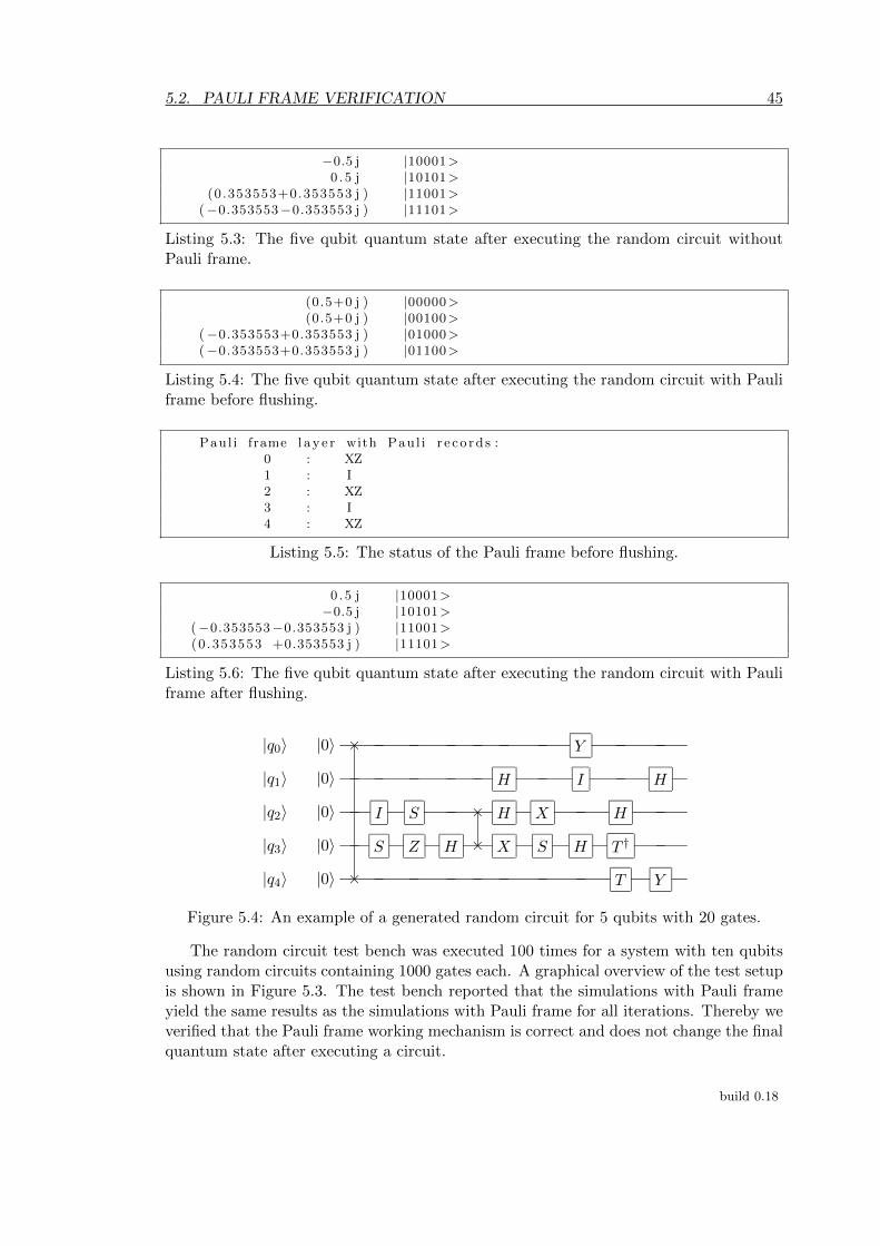
5.2. PAULI FRAME VERIFICATION 45

−0.5 j |10001>0 .5 j |10101>

(0 .353553+0.353553 j ) |11001>(−0.353553−0.353553 j ) |11101>

Listing 5.3: The five qubit quantum state after executing the random circuit withoutPauli frame.

(0.5+0 j ) |00000>(0.5+0 j ) |00100>

(−0.353553+0.353553 j ) |01000>(−0.353553+0.353553 j ) |01100>

Listing 5.4: The five qubit quantum state after executing the random circuit with Pauliframe before flushing.

Paul i frame l ay e r with Paul i r e co rd s :0 : XZ1 : I2 : XZ3 : I4 : XZ

Listing 5.5: The status of the Pauli frame before flushing.

0 .5 j |10001>−0.5 j |10101>

(−0.353553−0.353553 j ) |11001>(0 .353553 +0.353553 j ) |11101>

Listing 5.6: The five qubit quantum state after executing the random circuit with Pauliframe after flushing.

|q0〉 |0〉 × Y

|q1〉 |0〉 H I H

|q2〉 |0〉 I S × H X H

|q3〉 |0〉 S Z H × X S H T †

|q4〉 |0〉 × T Y

Figure 5.4: An example of a generated random circuit for 5 qubits with 20 gates.

The random circuit test bench was executed 100 times for a system with ten qubitsusing random circuits containing 1000 gates each. A graphical overview of the test setupis shown in Figure 5.3. The test bench reported that the simulations with Pauli frameyield the same results as the simulations with Pauli frame for all iterations. Thereby weverified that the Pauli frame working mechanism is correct and does not change the finalquantum state after executing a circuit.

build 0.18


5.2.3 Ninja star measurement simulation results

The Pauli frame layer is also tested in combination with the ninja star layer to verifythat measurements are handled correctly by the Pauli frame in case we do not flushthe Pauli frame. We used a control stack consisting of a ninja star layer, a Pauli framelayer, and a QxCore layer. A schematic overview of the test setup is shown in Figure5.5. To verify the measurement behavior of the control stack with a Pauli frame layer,we used a test bench that applies the circuit shown in Figure 5.6 to create the logicalstate (|01〉 + |10〉)/

√2 (which we will refer to as the odd Bell state) and measure the

outcome. The measurement results of multiple iterations are collected and plotted in ahistogram. The circuit to create the odd Bell state will be applied on the ninja star layerwhich expands all logical operations to physical operations and inserts ESM circuits.The explained test bench is relevant since the test procedure includes execution of Pauligates and measurements on the same qubits, which will test the measurement proceduresof the Pauli frame. None of the gates that will be executed due to the logical circuit orESM circuits are non-Clifford, which means that the none of the Pauli records will beflushed during execution.

Pauli Frame Layer

QX Simulator

QxCore

Test Bench

Ninja Star Layer

Figure 5.5: The test setup with a ninja star layer and a Pauli frame layer.

|q0〉 |0〉 H • XLL✙✙✙✙✙✙ ❴❴❴❴❴❴❴❴

✤✤✤✤✤✤✤

❴ ❴ ❴ ❴ ❴ ❴ ❴ ❴

✤✤✤✤✤✤✤

|q1〉 |0〉 ⊕LL✙✙✙✙✙✙ ❴❴❴❴❴❴❴❴

✤✤✤✤✤✤✤

❴ ❴ ❴ ❴ ❴ ❴ ❴ ❴

✤✤✤✤✤✤✤

Figure 5.6: The circuit used to create an odd Bell state.

The expected outcome of the odd Bell state test bench would be a histogram withequal frequencies at the states |01〉L and |10〉L. We performed the test bench with 100iterations on the test setup shown in Figure 5.5 and on a similar test setup without Pauliframe. Both tests yielded equivalent results and the resulting histograms are shown inFigure 5.7a and 5.7b for respectively the control stack with and without Pauli frame.We can conclude that both resulting histograms match the expected outcome. Hence,

build 0.18

5.3. NINJA STAR LOGICAL ERROR RATES 47

we can conclude that a system with a Pauli frame yields similar measurement results asa system without Pauli frame.

|00> |01> |10> |11>State after measurement

0

10

20

30

40

50

60

Freq

uenc

y

(a) Result with Pauli frame.

|00> |01> |10> |11>State after measurement

0

10

20

30

40

50

60

Freq

uenc

y

(b) Result without Pauli frame.

Figure 5.7: The resulting histograms of the odd Bell state test bench with and withoutPauli frame.

5.3 Ninja star logical error rates

The last experiment is designed to investigate the effect of the Pauli frame mechanismon QEC. To do so, we calculate the Logical Error Rate (LER) PL of an idling SurfaceCode 17 (SC17) logical qubit for different Physical Error Rate (PER) values p. The LERPL is defined as the probability of a logical error happening within a single window [19]where a window is defined as the time to execute one or more rounds of ESM and a setof required corrections after decoding the obtained error syndromes.

For a given p, PL can be calculated by simulation. In the simulation, a ninja star,constructed from 17 physical qubits, is initialized into the |0〉L or |+〉L state before werepeatedly perform ESM rounds without executing any logical operation. After everywindow, we check if there are any observable errors on data qubits, and if not, we checkif a logical error occurred. We repeat this procedure and count the number of windowsexecuted R and the number of logical errors detected m until m reaches a predefinedmaximum value. The LER PL corresponding to a given p can be written as:

PL|p =m

R(5.1)

Listing 5.7 contains a piece of pseudo code based on Python that summarizes the simu-lation procedure.

build 0.18


# I n i t i a l i z i n g used v a r i a b l e swindow count = 0l o g i c a l e r r o r c o u n t = 0

# I n i t i a l i z e the l o g i c a l qubiti n i t i a l i z e l o g i c a l q u b i t ( )

# Perform the experimentwhi l e l o g i c a l e r r o r c o u n t < MAX LOGICAL ERROR:

execute window ( )window count += 1

i f n o ob s e r v ab l e e r r o r s ( ) :i f l o g i c a l e r r o r h app en ed ( ) :

l o g i c a l e r r o r c o u n t += 1

# Calcu la t e the l o g i c a l e r r o r ra t el o g i c a l e r r o r r a t e = l o g i c a l e r r o r c o u n t / window count

Listing 5.7: Pseudo code summary of calculating the PL of a ninja star.

5.3.1 Test setup

We used QPDO to perform the LER experiments. We chose CHP as the simulationback-end to save simulation time since this experiment only executes Clifford gates. Thesymmetric depolarizing error model [11, 19] is used to insert errors and is implementedas a QPDO layer. The Pauli frame is also implemented as a layer as explained in Section5.2. Besides of the main layers required for the simulation, three counter layers are addedto the control stack to count the number of operations and time slots transferred betweenthe layers. The full control stack used for the LER experiments is shown in Figure 5.8.

The error layer implements the symmetric depolarizing error model. In this model,the PER p is the probability of an error occurring while executing a single operationon a physical qubit [11, 19]. For every single-qubit operation, the probability of a Paulierror, X, Y or Z, is for all p/3. Measurement in the computational basis can only havean X error with the probability of p. Idling a physical qubit for a time slot is alsotreated as a physical operation, the identity gate, I. For two-qubit gates the probabilityto insert a specific combination of two single-qubit errors is p/15 for all errors in the set({I,X, Y, Z} × {I,X, Y, Z}) \ {(I, I)}.

Error syndromes are the measurement result of the ancilla qubits and represent theparity among data qubits. A decoder is required to decode error syndromes into errorsthat happen on data qubits. For the LER experiments, the decoder used is a rule-basedLook-Up Table (LUT) decoder as presented in [19] and implemented by [37]. The rule-based LUT decoder is specifically designed for the ninja star and uses three rounds ofESM results to detect errors. Every window w uses one round of ESM results from theprevious window w − 1 as shown in Figure 5.9.

Detecting if there is any observable error in the data qubits is done by performing anextra round of ESM and verifying if the measurement results are all +1. This round ofESM used for diagnostic purposes should be error-free and not affect any counters in the

build 0.18


Pauli Frame Layer

CHP

ChpCore

Experiment with Pauli

frameCount Layer

Count Layer

Error Layer

Count Layer

Experiment without Pauli

frame

Figure 5.8: The test setup used for the Logical Error Rate experiments.

Corrections

ESM

ESM

Corrections

ESM

ESM

Corrections

ESM

...

...

Window

w

Window

w-1

Figure 5.9: The scheme of Error Syndrome Measurement (ESM) results used for succes-sive windows.

experiment. Therefore, apart from the normal execution mode, the control stack has abypass mode which is only valid for system diagnostics circuits where the counter layersand error layers are bypassed.

Logical errors are detected using stabilizer circuits in the bypass mode. We can usethe circuit shown in Figure 5.10a to verify if the ninja star is in the |0〉L/|1〉L state whichcorresponds to the ancilla measurement result +1/−1. The circuit shown in Figure 5.10ais a Z0Z4Z8 stabilizer measurement circuit and does not influence the logical |0〉L/|1〉Lstate of the ninja star [11]. By detecting changes of logical state after successive windows,

build 0.18


we can detectXL errors. For the same reason, ZL errors can be detected without affectingthe logical state using the stabilizer measurement circuit shown in Figure 5.10b withmeasurement result +1/−1 corresponding to the state |+〉L/|−〉L. More informationabout stabilizer circuits can be found in [6].

|d0〉 •

|d4〉 •

|d8〉 •

|a〉 |0〉 ⊕⊕⊕LL✙✙✙✙✙✙ ❴❴❴❴❴❴❴❴

✤✤✤✤✤✤✤

❴ ❴ ❴ ❴ ❴ ❴ ❴ ❴

✤✤✤✤✤✤✤

(a) Circuit for detecting XL errors.

|d2〉 ⊕

|d4〉 ⊕

|d6〉 ⊕

|a〉 |0〉 H • • • HLL✙✙✙✙✙✙ ❴❴❴❴❴❴❴❴

✤✤✤✤✤✤✤

❴ ❴ ❴ ❴ ❴ ❴ ❴ ❴

✤✤✤✤✤✤✤

(b) Circuit for detecting ZL errors.

Figure 5.10: The stabilizer circuits used to detect logical errors.

The ESM circuits for X and Z ancilla qubits, as described in Section 2.5.1, areperformed in parallel which results in an ESM circuit containing a total of 48 gatesdivided over 8 time slots including preparation and measurements of ancilla qubits.Table 5.8 describes which time slot contains which gates.

Time slot # Operations Short description

1 4 Reset X ancilla qubits to |0〉 state.

2 4 Reset Z ancilla qubits to |0〉 state.4 Apply H gates on X ancilla qubits.

3-6 24 CNOT gates between data qubits and ancilla qubits.

7 4 Apply H gates on X ancilla qubits.

8 8 Measure all ancilla qubits.

Table 5.8: Description of the Error Syndrome Measurement circuit used for the logicalerror rate experiment.

5.3.2 Results

We performed separate LER experiments for XL/ZL errors, starting from the |0〉L/|+〉Lstate, using the test setup shown in Figure 5.8 without Pauli frame. Both experimentswere performed for PER values ranging from 1.0× 10−4 to 1.00× 10−2 with a step sizeof 1.0 × 10−4 where ten simulations are performed for every PER. Every simulationis terminated when 50 logical errors are detected. For every PER, we calculated themean and standard deviation of the resulting LER of the ten individual simulations.The resulting graphs are shown in Figure 5.11 where the PER is represented on thehorizontal axis and the resulting LER on the vertical axis. We also added the line x = yand a vertical dashed line which indicates the intersection between the linear interpolatedresults and the line x = y.

build 0.18


10-4 10-3 10-2

Physical error rate

10-5

10-4

10-3

10-2

10-1Lo

gica

l err

or ra

te

(a) LER for logical X errors.

10-4 10-3 10-2

Physical error rate

10-5

10-4

10-3

10-2

10-1

Logi

cal e

rror

rate

(b) LER for logical Z errors.

Figure 5.11: Physical Error Rate versus Logical Error Rate for a Surface Code 17 logicalqubit without Pauli frame.

From the graphs shown in Figure 5.11 we can conclude that the LER is similar forXL and ZL errors, which can be explained by the used error model. The symmetricdepolarizing error model has equal probabilities for injecting X and Z errors on physicalqubits resulting in an equal probability of causing a logical X or Z error. Both graphsintersect the line x = y around x ≈ 3.0 × 10−4 which is marked with a vertical dashedline and known as the pseudo-threshold (as explained in Section 2.5.1). We performedan other set of similar simulations for PER values around the pseudo-threshold rangingfrom 3.0× 10−4 to 5.0× 10−4 with a step size of 5× 10−6 where 20 samples were takenfor every PER. The results are shown in Figure 5.12.

10-4 10-3

Physical error rate

10-4

10-3

Logi

cal e

rror

rate


10-4 10-3

Physical error rate

10-4

10-3

Logi

cal e

rror

rate


Figure 5.12: Physical Error Rate versus Logical Error Rate around the pseudo-thresholdfor a Surface Code 17 logical qubit without Pauli frame.

To observe the impact of a Pauli frame on the LER, we performed the same LERexperiments as explained earlier, but then using the test setup shown in Figure 5.8 witha Pauli frame. The graphs with the resulting LER values are shown in Figure 5.13.

build 0.18


Again we observe that the LER is similar for XL and ZL errors, which was expected.The pseudo-threshold, which is marked with a vertical dashed line, can again be foundaround 3.0 × 10−4. Again we performed extra simulations for PER values around thepseudo-threshold ranging from 3.0 × 10−4 to 5.0 × 10−4 of which the results are shownin Figure 5.14.

10-4 10-3 10-2

Physical error rate

10-5

10-4

10-3

10-2

10-1

Logi

cal e

rror

rate


10-4 10-3 10-2

Physical error rate

10-5

10-4

10-3

10-2

10-1

Logi

cal e

rror

rate


Figure 5.13: Physical Error Rate versus Logical Error Rate for a Surface Code 17 logicalqubit with Pauli frame.

10-4 10-3

Physical error rate

10-4

10-3

Logi

cal e

rror

rate


10-4 10-3

Physical error rate

10-4

10-3

Logi

cal e

rror

rate


Figure 5.14: Physical Error Rate versus Logical Error Rate around the pseudo-thresholdfor a Surface Code 17 logical qubit with Pauli frame.

We combined the results of the LER experiments with and without Pauli frame inone figure to be able to compare them. The results of the experiments performed overthe range 1.0 × 10−4 to 1.00 × 10−2 are shown in Figure 5.16 while the results of thesimulations around the pseudo-threshold of 3.0× 10−4 are shown in Figure 5.16. Againthe results with Pauli frame are indicated with red circles while the results withoutPauli frame are indicated by blue squares. By visual inspection, we can conclude thatthe results of the LER experiments with Pauli frame look very similar to the results

build 0.18


of the experiments without Pauli frame. Our observed results are also very similar tothe results shown in [19] where they assume the presence of a Pauli frame during theirsimulations.

10-4 10-3 10-2

Physical error rate

10-5

10-4

10-3

10-2

10-1

Logi

cal e

rror

rate


10-4 10-3 10-2

Physical error rate

10-5

10-4

10-3

10-2

10-1

Logi

cal e

rror

rate


Figure 5.15: Physical Error Rate versus Logical Error Rate for a Surface Code 17 logicalqubit with (red circles) and without (blue squares) Pauli frame.

10-4 10-3

Physical error rate

10-4

10-3

Logi

cal e

rror

rate


10-4 10-3

Physical error rate

10-4

10-3

Logi

cal e

rror

rate


Figure 5.16: Physical Error Rate versus Logical Error Rate for a Surface Code 17 logicalqubit with (red circles) and without (blue squares) Pauli frame around the pseudo-threshold.

To take a closer look at the differences between the results with and without Pauliframe we calculated the absolute difference in LER δPL

for every PER p where δPLis

defined as:

δPL|p = PLwithout PF

− PLwith PF(5.2)

Figure 5.17 shows the absolute LER difference δPL(red triangles) for every p on a sym-

metric logarithmic scale where the vertical axis has a logarithmic scale except between±10−4 where the scale is linear. The δPL

for the results of the simulations around the

build 0.18


pseudo-threshold are shown in Figure 5.18 with a symmetric logarithmic scale on thevertical axis that is linear between ±10−5. In the plots for δPL

, the maximum of thestandard deviations of PL with and without Pauli frame σmax was added around thehorizontal axis for every p where for a given p, σmax is defined as:

σmax|p = max(σ(PLwith PF

) , σ(PLwithout PF))

(5.3)

From Figure 5.17 and 5.18 we can observe that there is no consistent positive or negativedifference in LER PL for the simulations with and without Pauli frame. Also for nearlyall p, δPL

can be found within the standard deviation regions ±σmax. We can concludethat the Pauli frame has no measurable effect on the LER of a SC17 logical qubit.

10-4 10-3 10-2

Physical error rate

-10-1

-10-2

-10-3

-10-4

0

10-4

10-3

10-2

10-1

Abso

lute

impr

ovem

ent l

ogic

al e

rror

rate

by

Paul

i fra

me

(a) Difference for logical X errors.

10-4 10-3 10-2

Physical error rate

-10-1

-10-2

-10-3

-10-4

0

10-4

10-3

10-2

10-1

Abso

lute

impr

ovem

ent l

ogic

al e

rror

rate

by

Paul

i fra

me

(b) Difference for logical Z errors.

Figure 5.17: The absolute Logical Error Rate difference between the experiments withand without Pauli frame (red triangles) plotted together with the standard deviationsof the LER results (vertical bars).

We might wonder why the maximum standard deviations of the LER plotted inFigure 5.17 and 5.18 increase for higher PER values p. We know from Equation (5.1)that the LER PL depends on the number of detected logical errors m and the number ofcounted windows R. The simulations we perform are always terminated when m = 50,which means that PL can only be influenced by R. For a given p we would like to knowthe coefficient of variation (also known as the relative standard deviation) c of R whichis defined as:

cR|p =σRµR

(5.4)

We calculated the cR for every p and the results for the simulations with and withoutPauli frame are shown in Figure 5.19 and 5.20 in red and blue. We can observe that forsimulations with and without Pauli frame the average of cR lies around 13% for all pwhich are marked with horizontal dashed lines. We can conclude that for every p, R hasa relative standard deviation around 13%, which will result in a proportional coefficientof variation for PL. Since PL is larger for larger p, the absolute standard deviation forPL will be greater for higher values of p. Hence, we observe larger absolute standarddeviations for larger p in Figure 5.17 and 5.18.

build 0.18


10-4 10-3

Physical error rate

-10-3

-10-4

-10-5

0

10-5

10-4

10-3Ab

solu

te im

prov

emen

t log

ical

err

or ra

te b

y Pa

uli f

ram

e

(a) Difference for logical X errors.

10-4 10-3

Physical error rate

-10-3

-10-4

-10-5

0

10-5

10-4

10-3

Abso

lute

impr

ovem

ent l

ogic

al e

rror

rate

by

Paul

i fra

me

(b) Difference for logical Z errors.

Figure 5.18: The absolute Logical Error Rate difference between the experiments withand without Pauli frame (red triangles) plotted together with the standard deviationsof the LER results (vertical bars) around the pseudo-threshold.

10-4 10-3 10-2

Physical error rate

0.04

0.06

0.08

0.10

0.12

0.14

0.16

0.18

0.20

0.22

Coef

ficie

nt o

f var

iatio

n of

win

dow

cou

nt

(a) During LER simulations for XL errors.

10-4 10-3 10-2

Physical error rate

0.02

0.04

0.06

0.08

0.10

0.12

0.14

0.16

0.18

0.20

Coef

ficie

nt o

f var

iatio

n of

win

dow

cou

nt

(b) During LER simulations for ZL errors.

Figure 5.19: The coefficient of variation of the number of counted windows with (redcircles) and without (blue squares) Pauli frame.

We also performed statistical analysis on the LER samples retrieved by individualsimulations. For every PER p we performed a t-test which can indicate if two data setsare significantly different from each other by calculating a ρ-value. A consistent ρ-valueof 0.05 or lower would indicate that the difference between two sets of data is statisticallysignificant. If not, the null hypothesis holds which indicates that the difference betweentwo sets of data is not statistically significant. For a given p, we used one data set withLER values obtained by simulations without Pauli while the other data set contained theLER values obtained by simulations with Pauli frame. As mentioned earlier, simulationswith and without Pauli frame were repeated 10 times for every p which means that thetwo data sets that we compare both have a sample size of 10. The t-test can be performedon matched pairs (paired t-test) or independent data sets (unpaired or independent t-

build 0.18


10-4 10-3

Physical error rate

0.06

0.08

0.10

0.12

0.14

0.16

0.18

Coef

ficie

nt o

f var

iatio

n of

win

dow

cou

nt

(a) During LER simulations for XL errors.

10-4 10-3

Physical error rate

0.08

0.10

0.12

0.14

0.16

0.18

0.20

Coef

ficie

nt o

f var

iatio

n of

win

dow

cou

nt

(b) During LER simulations for ZL errors.

Figure 5.20: The coefficient of variation of the number of counted windows with (redcircles) and without (blue squares) Pauli frame around the pseudo-threshold.

test). The LER samples obtained by our simulations are not paired for simulationswith and without Pauli frame which would indicate the usage of an independent t-test,but all simulations do use the same simulation software which could imply that we aretesting the same object and suggest the usage of a paired t-test. For those reasons,we performed both the paired as well as the independent t-test. The resulting ρ-valuesof the independent t-test for every p for simulations considering XL and ZL errors areshown in Figure 5.21 and the results for the same data using the paired t-test are shownin Figure 5.22. Figures 5.23 and 5.24 present the results of the individual and pairedt-test performed on the data obtained by simulations around the pseudo-threshold whereevery data set has a sample size of 20. All graphs also contain a horizontal dashed lineto indicate the mean of the ρ-values in the graph.

10-4 10-3 10-2

Physical error rate

0.0

0.2

0.4

0.6

0.8

1.0

p-va

lue

(a) ρ-values for data obtained by simulationsfor XL errors.

10-4 10-3 10-2

Physical error rate

0.0

0.2

0.4

0.6

0.8

1.0

p-va

lue

(b) ρ-values for data obtained by simulationsfor ZL errors.

Figure 5.21: The resulting ρ-values from the independent t-test performed on the datasets obtained with and without Pauli frame for different Physical Error Rate values.

build 0.18


10-4 10-3 10-2

Physical error rate

0.0

0.2

0.4

0.6

0.8

1.0p-

valu

e


10-4 10-3 10-2

Physical error rate

0.0

0.2

0.4

0.6

0.8

1.0

p-va

lue


Figure 5.22: The resulting ρ-values from the paired t-test performed on the data setsobtained with and without Pauli frame for different Physical Error Rate values.

10-4 10-3

Physical error rate

0.0

0.2

0.4

0.6

0.8

1.0

p-va

lue


10-4 10-3

Physical error rate

0.0

0.2

0.4

0.6

0.8

1.0

p-va

lue


Figure 5.23: The resulting ρ-values from the independent t-test performed on the datasets obtained with and without Pauli frame for different Physical Error Rate values.

From the results of the t-tests shown in Figure 5.21, 5.22, 5.23, and 5.24 we canobserve that the ρ-values vary a lot for different values of p and that the mean of all ρ-values lies around 0.5. Although we see a few ρ-values lower than 0.05 we do not observesuch values consistently over many values of p. By conventional criteria, the differencebetween the data sets obtained with and without Pauli frame is considered to be notstatistically significant. Hence, we can conclude that the Pauli frame has no statisticallysignificant effect on the LER of a SC17 logical qubit.

To investigate why the usage of a Pauli frame does not significantly influence theLER we have taken a look at the gate and time slot counts that we collected during thesimulations. We were especially interested in the number of Pauli gates that were filtered

build 0.18


10-4 10-3

Physical error rate

0.0

0.2

0.4

0.6

0.8

1.0

p-va

lue


10-4 10-3

Physical error rate

0.0

0.2

0.4

0.6

0.8

1.0

p-va

lue


Figure 5.24: The resulting ρ-values from the paired t-test performed on the data setsobtained with and without Pauli frame for different Physical Error Rate values aroundthe pseudo-threshold.

by the Pauli frame and the number of time slots that were removed as a result of that.An ESM circuit as shown in Table 5.8 does not contain any Pauli gate, so the only gatesthat can be filtered are Pauli gates that were inserted correct errors. A window consistsof two rounds of ESM and one possible time slot for corrections. Every ESM round has8 time slots resulting in a total of 2 · 8 = 16 time slots per window. As a result, a singlewindow can have 16 or 17 time slots depending on if there are corrections to be appliedor not. The only time slot that could potentially be filtered by the Pauli frame is thetime slot containing the correction gates. If corrections are applied at the end of everywindow, 1/17 ≈ 0.06 or around 6% of the time slots could be filtered by the Pauli frame.As a result, the Pauli frame can never filter more than 6% of the time slots during oursimulations. For all simulations regarding logical X errors, we calculated the percentageof gates and time slots that were filtered by the Pauli frame. We calculated the mean andstandard deviation of these results for every PER p and the resulting graphs are shownin Figure 5.25. We also calculated the percentage of filtered gates and time slots for thesimulations regarding logical X errors around the pseudo-threshold. Those results areshown in Figure 5.26.

From the graphs shown in Figure 5.25 and 5.26 we can conclude that the Pauli framedoes filter gates and time slots, but the percentage of gates and time slots that arefiltered is low, especially for PER values below the pseudo-threshold. These results canbe explained by the distance d. For the SC17, distance d = 3 which means that the SC17is able to correct (d− 1)/2 = 1 error per ESM round. As a result, the pseudo-thresholdof the SC17 is found at a very low PER. Due to the low PER and low distance of theSC17, there is a very low number of corrections to be applied over time, which resultsin a low number of gates and time slots being filtered by the Pauli frame.

The low proportion of gates and time slots that are filtered by the Pauli frame canalso explain why we do not see any improvements in the LER by using a Pauli frame.

build 0.18


10-4 10-3 10-2

Physical error rate

0.0

0.2

0.4

0.6

0.8

1.0

1.2

1.4Sa

ved

oper

atio

ns in

%

(a) Percentage of saved gates.

10-4 10-3 10-2

Physical error rate

0

1

2

3

4

5

Save

d tim

e sl

ots

in %

(b) Percentage of saved time slots.

Figure 5.25: The percentage of gates and time slots saved by the Pauli frame duringLogical Error Rate simulations for X errors.

10-4 10-3

Physical error rate

0.050

0.055

0.060

0.065

0.070

0.075

0.080

0.085

0.090

Save

d op

erat

ions

in %

(a) Percentage of saved gates.

10-4 10-3

Physical error rate

0.25

0.30

0.35

0.40

0.45

0.50Sa

ved

time

slot

s in

%

(b) Percentage of saved time slots.

Figure 5.26: The percentage of gates and time slots saved by the Pauli frame duringLogical Error Rate simulations for X errors around the pseudo-threshold.

Improvements in the LER due to a Pauli frame can only be observed if a significantproportion of time slots is filtered. Since only a very low percentage of time slots isfiltered at PER values below the pseudo-threshold, no improvement in the LER can beobserved. For PER values above the pseudo-threshold the percentage of filtered timeslots increases quickly, but still, we do not observe any improvement in LER. At PERvalues above the pseudo-threshold, the SC17 suffers from more errors than it can correct.Logical errors occur often, and a Pauli frame can not prevent that. Hence, we can notobserve improvements in the LER at PER values above the pseudo-threshold.

We might wonder if we can expect improved LER values for a surface code witha larger distance d > 3 using a Pauli frame. Therefore, we need to look further intothe theoretical benefit a Pauli frame can gain for the LER. The following reasoning isnot meant as an analytical proof but rather a quantitative reasoning about the relative

build 0.18


impact of both the Pauli frame and the code distance on the LER.

Given a PER p, we could approximate the LER PL based on the distance d, andthe number of time slots required by a single window tswindow. We know that tswindow

equals the sum of the time slots required by d− 1 rounds of ESM tsrounds and the timeslot for corrections tscorrections. In our simulations, the number of time slots in a singleround of ESM tsESM = 8 as shown in Table 5.8. For the surface code, PL is negativelycorrelated to the code distance d. Given the same PER and surface code lattice witha certain distance, more time slots required by a window would lead to more physicalerrors occurring per window, which could further increase the LER. Hence, we canassume that the LER is positively correlated to the number of time slots required by awindow. Given a PER p, it would be a reasonable assumption to estimate the LER PLby Equation (5.5):

PL|p ∝ tswindow

d(5.5)

where

tswindow = tsrounds + tscorrections (5.6)

tsrounds = (d− 1)tsESM (5.7)

tsESM = 8 (5.8)

tscorrections =

{1 if there are errors to be corrected

0 otherwise(5.9)

We can improve the LER PL by reducing tswindow using a Pauli frame. The Pauliframe can track all detected errors and as a result the value of tscorrections is reducedto tscorrections = 0. Given a tsESM, let us calculate the upper-bound for the relativeimprovement in PL that we can obtain by using a Pauli frame. Based on Equation (5.5)we will approximate PL with/without Pauli frame as shown in Equation (5.10)/(5.11)where C is a constant:

C · tswindow

d

∣∣∣∣PF

where tscorrections = 0 (with Pauli frame) (5.10)

C · tswindow

d

∣∣∣∣wo PF

where tscorrections = 1 (without Pauli frame) (5.11)

build 0.18


Now we can define the upper-bound for the relative improvement in PL as:

Brelative ∝C · tswindow

d

∣∣∣∣wo PF

− C · tswindow

d

∣∣∣∣PF

C · tswindow

d

∣∣∣∣wo PF

=tswindow|wo PF − tswindow|PF

tswindow|wo PF

=1

tswindow|without PF

=1

(d− 1)tsESM + 1

(5.12)

From Equation (5.12), we can conclude that the upper-bound for the relative improve-ment in LER that can be obtained by using a Pauli Frame converges to 0 for a largedistance d and for a large tsESM. We plotted Equation (5.12) for tsESM = 8 in Figure5.27 and we can observe that the upper-bound on the relative improvement quickly de-creases to values below 3%. Hence, we do not expect an improved LER that for a largerdistance d by using a Pauli frame.

3 4 5 6 7 8 9 10 11Distance

0

1

2

3

4

5

6

Uppe

r-bou

nd re

lativ

e im

prov

emen

t in

%

Figure 5.27: The upper-bound on the relative improvement in Logical Error Rate thatcan be obtained by using a Pauli frame for tsESM = 8.

build 0.18


build 0.18

Conclusion 6We have analyzed the working principles of Pauli frames in detail and created an im-plementation using the QPDO software. Our simulations show that when executing thesame circuits, a quantum system with a Pauli frame does yield the same measurementresults as a quantum system without a Pauli frame. We have also shown that by trackingPauli operations instead of executing them, we are still able to restore the quantum stateto the state it would have been without the usage of a Pauli frame. For those reasonsit is possible to add a Pauli frame to a quantum system while still yielding the sameresults, even when the usage of a Pauli frame causes fewer gates being applied on itscorresponding qubits.

We have also verified the logical operations of the Surface Code 17 (SC17) by simula-tion. The verified logical operations include preparation to |0〉L, XL, ZL, HL, transversalCNOTL, transversal CZL, and nine-qubit measurement in the ZL basis. In our simula-tions, we preferred to use the nine-qubit measurement over the three-qubit measurementsince lattice rotation does not influence the former.

We have shown that the usage of a Pauli frame does not cause an observable improve-ment on the Logical Error Rate (LER) of a SC17, even when the Pauli frame effectivelyfilters all gates required to correct errors. By doing further analysis, we concluded thata surface code with a larger distance might also not benefit from an improved LER bythe usage of a Pauli frame. Nevertheless, by using a Pauli frame we can still benefit fromrelaxed timing constraints for error decoding and Error Syndrome Measurement (ESM)circuit execution time.

Functional simulations have shown that our proposed design for a quantum computerarchitecture targeting a SC17 quantum chip can maintain a logical qubit. Our archi-tecture is capable of performing Quantum Error Correction (QEC) and can scheduleconverted logical operations for execution.

Finally, we can conclude that the QPDO software is very flexible and offers powerfulsimulation capabilities. The combination of a layered structure combined with differ-ent simulation back-ends has proven to be very useful, especially in conjunction withautomated test benches. All simulations required for this report, and more, have beenperformed with success using QPDO.

Future work

The work in this thesis could be extended in different directions.

We verified a set of logical operations for a SC17 logical qubit, but it would beinteresting to extend the set of operations. In [14] a procedure for state injection wasproposed that would make it possible to extend the set of logical gates for the SC17. Itmight also be interesting to look at different techniques to encode logical qubits using

63

64 CHAPTER 6. CONCLUSION

the surface code (e.g. defect-based logical qubits as discussed in [6]) and verify thecorresponding logical operations.

The experiments considering the effect of a Pauli frame on the LER of a SC17 canalso be extended. It would be interesting to repeat these experiment using a largerdistance surface code to verify our expectations that for a larger distance surface code,there will be no benefit in LER by using a Pauli frame. Such simulations would in thefirst place require error syndrome decoders that are suitable for larger surface codes.Future simulations could also benefit from more realistic error models.

Finally, we would like to take a deeper look into our proposed quantum computerarchitecture [34]. Interesting work could be done by performing more accurate simula-tions of the quantum computer architecture up to a level where we perform clock-cycleaccurate emulation.

build 0.18

Bibliography

[1] P. W. Shor, “Algorithms for quantum computation: Discrete logarithms and fac-toring,” in Foundations of Computer Science, 1994 Proceedings., 35th Annual Sym-posium on, pp. 124–134, IEEE, 1994.

[2] L. K. Grover, “Quantum mechanics helps in searching for a needle in a haystack,”Physical review letters, vol. 79, no. 2, p. 325, 1997.

[3] D. Riste, S. Poletto, M. Z. Huang, et al., “Detecting bit-flip errors in a logical qubitusing stabilizer measurements,” Nat Commun, vol. 6, 04 2015.

[4] A. Corcoles et al., “Demonstration of a quantum error detection code using a squarelattice of four super-conducting qubits,” Nature Comm., vol. 6, 2015.

[5] J. Kelly et al., “State preservation by repetitive error detection in a superconductingquantum circuit,” Nature, vol. 519, no. 7541, pp. 66–69, 2015.

[6] A. G. Fowler, M. Mariantoni, J. M. Martinis, and A. N. Cleland, “Surface codes:Towards practical large-scale quantum computation,” Physical Review A, vol. 86,no. 3, p. 032324, 2012.

[7] P. W. Shor, “Scheme for reducing decoherence in quantum computer memory,”Physical review A, vol. 52, no. 4, p. R2493, 1995.

[8] E. Knill, “Quantum computing with realistically noisy devices,” Nature, vol. 434,no. 7029, pp. 39–44, 2005.

[9] N. Khammassi, “QX simulator.” http://www.xpu-project.net/qx/download.

html, 2016. Universal quantum simulator developed by the Computer Engineer-ing department of Delft University of Technology.

[10] S. Aaronson and D. Gottesman, “Improved simulation of stabilizer circuits,” Phys-ical Review A, vol. 70, no. 5, p. 052328, 2004.

[11] M. A. Nielsen and I. L. Chuang, Quantum computation and quantum information.Cambridge university press, 2010.

[12] B. M. Terhal, “Quantum error correction for quantum memories,” Reviews of Mod-ern Physics, vol. 87, no. 2, p. 307, 2015.

[13] A. Y. Kitaev, “Fault-tolerant quantum computation by anyons,” Annals of Physics,vol. 303, no. 1, pp. 2–30, 2003.

[14] C. Horsman, A. G. Fowler, S. Devitt, and R. Van Meter, “Surface code quantumcomputing by lattice surgery,” New Journal of Physics, vol. 14, no. 12, p. 123011,2012.

65

http://www.xpu-project.net/qx/download.html

http://www.xpu-project.net/qx/download.html

66 BIBLIOGRAPHY

[15] A. G. Fowler, A. M. Stephens, and P. Groszkowski, “High-threshold universal quan-tum computation on the surface code,” Physical Review A, vol. 80, no. 5, p. 052312,2009.

[16] E. Dennis, A. Kitaev, A. Landahl, and J. Preskill, “Topological quantum memory,”Journal of Mathematical Physics, vol. 43, no. 9, pp. 4452–4505, 2002.

[17] N. C. Jones, R. Van Meter, A. G. Fowler, P. L. McMahon, J. Kim, T. D. Ladd, andY. Yamamoto, “Layered architecture for quantum computing,” Physical Review X,vol. 2, no. 3, p. 031007, 2012.

[18] S. J. Devitt, W. J. Munro, and K. Nemoto, “Quantum error correction for begin-ners,” Reports on Progress in Physics, vol. 76, no. 7, p. 076001, 2013.

[19] Y. Tomita and K. M. Svore, “Low-distance surface codes under realistic quantumnoise,” Physical Review A, vol. 90, no. 6, p. 062320, 2014.

[20] Y.-C. Zheng and T. A. Brun, “Fault-tolerant holonomic quantum computation insurface codes,” Physical Review A, vol. 91, no. 2, p. 022302, 2015.

[21] M. Takita, A. Corcoles, E. Magesan, B. Abdo, M. Brink, A. Cross, J. M. Chow, andJ. M. Gambetta, “Demonstration of weight-four parity measurements in the surfacecode architecture,” arXiv preprint arXiv:1605.01351, 2016.

[22] J. Kelly, R. Barends, A. Fowler, A. Megrant, E. Jeffrey, T. White, D. Sank, J. Mutus,B. Campbell, Y. Chen, et al., “State preservation by repetitive error detection in asuperconducting quantum circuit,” Nature, vol. 519, no. 7541, pp. 66–69, 2015.

[23] M. B. Hastings and A. Geller, “Reduced space-time and time costs using dislocationcodes and arbitrary ancillas,” arXiv preprint arXiv:1408.3379, 2014.

[24] J. Edmonds, “Maximum matching and a polyhedron with 0, l-vertices,” J. Res.Nat. Bur. Standards B, vol. 69, no. 1965, pp. 125–130, 1965.

[25] J. Edmonds, “Paths, trees, and flowers,” Canadian Journal of mathematics, vol. 17,no. 3, pp. 449–467, 1965.

[26] E. Knill, “Scalable quantum computing in the presence of large detected-errorrates,” Physical Review A, vol. 71, no. 4, p. 042322, 2005.

[27] D. P. DiVincenzo and P. Aliferis, “Effective fault-tolerant quantum computationwith slow measurements,” Physical review letters, vol. 98, no. 2, p. 020501, 2007.

[28] P. Aliferis and J. Preskill, “Fault-tolerant quantum computation against biasednoise,” Physical Review A, vol. 78, no. 5, p. 052331, 2008.

[29] A. JavadiAbhari, S. Patil, D. Kudrow, J. Heckey, A. Lvov, F. T. Chong, andM. Martonosi, “Scaffcc: A framework for compilation and analysis of quantumcomputing programs,” in Proceedings of the 11th ACM Conference on ComputingFrontiers, p. 1, ACM, 2014.

build 0.18

BIBLIOGRAPHY 67

[30] S. Balensiefer, L. Kregor-Stickles, and M. Oskin, “An evaluation framework and in-struction set architecture for ion-trap based quantum micro-architectures,” in ACMSIGARCH Computer Architecture News, vol. 33, pp. 186–196, IEEE Computer So-ciety, 2005.

[31] K. M. Svore, A. V. Aho, A. W. Cross, I. Chuang, and I. L. Markov, “A layeredsoftware architecture for quantum computing design tools,” Computer, no. 1, pp. 74–83, 2006.

[32] D. Wecker and K. M. Svore, “Liqui—¿: A software design architecture and domain-specific language for quantum computing,” arXiv preprint arXiv:1402.4467, 2014.

[33] K. Svore, A. Cross, A. Aho, I. Chuang, and I. Markov, “Toward a software architec-ture for quantum computing design tools,” in Proceedings of the 2nd InternationalWorkshop on Quantum Programming Languages (QPL), pp. 145–162, 2004.

[34] X. Fu, L. Riesebos, L. Lao, C. Almudever, F. Sebastiano, R. Versluis, E. Charbon,and K. Bertels, “A heterogeneous quantum computer architecture,” in Proceedingsof the ACM International Conference on Computing Frontiers, pp. 323–330, ACM,2016.

[35] D. Iorga, “Python wrapper for CHP,” 2016. Wrapper to enable quantum simulationswith CHP using function calls from Python.

[36] H. Zimmermann, “OSI reference model–the iso model of architecture for open sys-tems interconnection,” Communications, IEEE Transactions on, vol. 28, no. 4,pp. 425–432, 1980.

[37] S. Varsamopoulos, “Rule-based lookup table decoder,” 2016. Python implementa-tion of the rule-based lookup table decoder.

build 0.18

68 BIBLIOGRAPHY

build 0.18

pauli frames for quantum computer architectures

Documents