Payments Infrastructure and the Performance of PublicPrograms: Evidence from Biometric Smartcards in India∗

Karthik Muralidharan†

UC San DiegoPaul Niehaus‡

UC San DiegoSandip Sukhtankar§

Dartmouth College

February 27, 2014

Abstract

Anti-poverty programs in developing countries are often implemented poorly, partly due tothe lack of a secure infrastructure to deliver payments to targeted beneficiaries. We evaluate theimpact of biometrically-authenticated payments infrastructure on public employment and pensionprograms in the Indian state of Andhra Pradesh. The unusual scale of our experiment, whichrandomized rollout over 158 sub-districts and 19 million people, lets us capture both the manage-ment challenges and general equilibrium effects that accompany real-world implementation. Wefind that, while far from perfectly implemented, the new technology delivered a faster, more pre-dictable, and less corrupt payments process without adversely affecting program access. Strikingly,we see large income gains for participants driven primarily by increases in private sector wages.This likely reflects an increase in the value of the public employment scheme as an outside op-tion, due to better implementation. The new payment system was cost-effective, as time savingsto beneficiaries alone were equal to the cost of the intervention in the case of the employmentscheme. Our results suggest that investing in secure authentication and payment infrastructurecan significantly enhance “state capacity” in developing countries to effectively implement a broadrange of welfare programs.

JEL codes: D73, H53, J43, O30

Keywords: biometric authentication, secure payments, electronic benefit transfers, public pro-grams, corruption, service delivery, general equilibrium effects, India

∗PRELIMINARY. PLEASE DO NOT CITE OR CIRCULATE WITHOUT AUTHORS’ CONSENT. We thankGordon Dahl, Gordon Hanson, Anh Tran, and several seminar participants for comments and suggestions. We aregrateful to officials of the Government of Andhra Pradesh, including Reddy Subrahmanyam, Koppula Raju, ShamsherSingh Rawat, Raghunandan Rao, G Vijaya Laxmi, AVV Prasad, Kuberan Selvaraj, Sanju, Kalyan Rao, and MadhaviRani; as well as Gulzar Natarajan for their continuous support of the Andhra Pradesh Smartcard Study. We are alsograteful to officials of the Unique Identification Authority of India (UIDAI) including Nandan Nilekani, Ram SevakSharma, and R Srikar for their support. We thank Tata Consultancy Services (TCS) and Ravi Marri, Ramanna,and Shubra Dixit for their help in providing us with administrative data. This paper would not have been possiblewithout the continuous efforts and inputs of the J-PAL/IPA project team including Kshitij Batra, Prathap Kasina,Piali Mukhopadhyay, Raghu Kishore Nekanti, Matt Pecenco, Surili Sheth, and Pratibha Shrestha. Finally, we thankthe Omidyar Network – especially Jayant Sinha, CV Madhukar, Surya Mantha, Ashu Sikri, and Dhawal Kothari – forthe financial support that made this study possible.†UC San Diego, JPAL, NBER, and BREAD. kamurali@ucsd.edu.‡UC San Diego, JPAL, NBER, and BREAD. pniehaus@ucsd.edu.§Dartmouth College, JPAL, and BREAD. sandip.sukhtankar@dartmouth.edu.

1

1 Introduction

Sending and receiving money securely across space is fundamental to the scale and scope of

an economy. Developed countries today are unusual in that their banking infrastructure

and legal environments allow for relatively seamless remote transactions: mail order,

online shopping, money wires, Electronic Benefit Transfers, and so on. In most times and

places, however, payments infrastructure was (is) less advanced. Payments often move

through informal networks (for example, the Maghribi traders studied by Greif (1993) or

the present-day “hawala” system in South Asia and the Middle East) or not at all. In the

public sector, weak payments infrastructure makes it difficult to deliver fast and reliable

payments to transfer recipients, and can create opportunities for graft. Reinikka and

Svensson (2004) and Niehaus and Sukhtankar (2013a,b) document forms of corruption,

for example, in which government officials simply steal funds meant for the poor, rather

then delivering them to the intended recipient. A secure payments infrastructure can thus

be seen as a form of “state capacity” that improves the state’s ability to implement its

welfare policies more effectively and expands its long-term policy choice set (Besley and

Persson, 2009, 2010). More broadly, it can be considered as public infrastructure, akin to

roads, railways, or the internet, that may have initially been set up by governments for

their own use (such as moving troops to the border quickly, or improving intra-government

communication), but eventually generated substantial spillovers to the private sector as

well.

Given the primacy of payments it is understandable that recent advances in payments

technology have generated considerable optimism regarding their ability to improve the

performance of public welfare programs.1 This is nowhere more true than in India. The

Indian government embarked in 2009 on an ambitious two-step agenda: deliver unique,

biometric-linked IDs to all 1.2 billion residents via the Aadhaar (“foundation”) initia-

tive, and then introduce Direct Benefit Transfers for social program beneficiaries using

Aadhaar-linked bank accounts.2 The Unique ID Authority of India has argued that “Aad-

haar will empower poor and underprivileged residents in accessing services such as the

formal banking system and give them the opportunity to easily avail various other services

provided by the Government and the private sector.”3 Finance Minister P. Chidambaram

has simply said that the project would be “a game changer for governance.”4

1The Better than Cash Alliance advocates for the adoption of electronic payments on the grounds thatthey “advance financial inclusion and cost savings while giving governments a more efficient, transparent andsecure means of disbursing benefit,” for example. See http://betterthancash.org/, accessed 29 January2014.

2Malaysia, South Africa, and Indonesia have similar pilot programs under way.3http://uidai.gov.in/index.php?option=comcontent&view=article&id=58&Itemid=106, accessed

September 10, 20134http://www.nytimes.com/2013/01/06/world/asia/india-takes-aim-at-poverty-with-cash-transfer-program.

html, accessed 3 October 2013.

2

At the same time, this optimism has also been tempered by skepticism regarding

the likely impact of such a system and whether it warrants the considerable cost and

administrative attention entailed. Concerns have been raised regarding (a) the extent of

the technical and logistical implementation challenges and the risk that such a complex

project will fail unless all components are implemented well (b) the possibility of political

vested interests subverting the corruption-reducing intent of the program (c) exclusion

errors whereby genuine beneficiaries are denied payments due to technical unreliablity of

the new system, which may lead to the most vulnerable beneficiaries being worse off even

if average outcomes improve (d) the possibility that reducing rents for local officials may

paradoxically hurt the rural poor by dampening the incentives for officials to implement

the anti-poverty programs in the first place, and (e) the cost effectiveness of the project.

This paper evaluates whether the game is in fact changing by measuring both potential

positive and negative impacts of a large-scale rollout of biometric payments infrastructure

integrated into social programs in India. Working with the Government of the Indian

state of Andhra Pradesh, we randomized the order in which 158 sub-districts introduced

biometrically-authenticated electronic benefit transfers into two large social programs: the

Mahatma Gandhi National Rural Employment Guarantee Scheme (NREGS for short) and

Social Security Pensions (SSP). The intervention, which we refer to as “Smartcards” for

short, provided beneficiaries with the same effective functionality that Aadhaar-enabled

Direct Benefit Transfers are intended to. The experiment thus provides an opportunity

to learn about the likely impacts of Aadhaar, and of modernized payments infrastructure

more generally. Further, the experiment randomized the form of payments over a uni-

verse of about 19 million people, with randomization conducted over entire sub-districts,

making it one of the largest randomized controlled trials ever conducted.

Evaluating an “as is” implementation of a complex program by a government at this

scale offers several unique advantages. First, our estimates correctly reflect the challenges

that accompany implementation at scale. In our context these include everything from

mundane logistics (e.g. capturing biometrics and delivering ID cards, procuring and

deploying authentication devices and ensuring their functioning, appointing new payment

agents, and cash management and security) to resistance from vested interests with a stake

in maintaining the status quo (Prescott and Parente, 2000), and our estimated treatment

effects are net of all of these. This addresses one common concern about randomized

trials in developing countries that study NGO-led pilots which may not provide accurate

forecasts of performance at the scales relevant for policy-making (see for example Bold

et al. (2013)).

Second, evaluating at scale lets us capture both direct effects on program performance

and also indirect, general equilibrium effects. Acemoglu (2010) among others has voiced

concern that “the bulk of empirical work using microdata, particularly in development

3

economics, engages in partial equilibrium comparisons” and thus cannot capture first-

order effects of full-scale implementation. These are likely to be particularly important in

our context. Employment guarantee schemes such as the NREGS compete directly with

private sector employers for labor, and there is some evidence that the NREGS rollout

increased private-sector wages (Imbert and Papp, 2012; Berg et al., 2012). Improving

the functioning of the NREGS by modernizing government payments delivery could thus

have spillover impacts on local labor markets. By randomizing large geographic units

into treatment and control arms we are able to capture these spillover effects.

We first characterize implementation, using both official micro-records and original

data from representative baseline and endline surveys of 7382 and 8172 households, respec-

tively. We find that after two years of program rollout, the share of Smartcard-enabled

payments in treated sub-districts had 50%. The incomplete conversion of treatment sub-

districts to the new payment system reflected a broad range of implementation frictions

that impeded program roll-out including logistical challenges in enrolling beneficiaries

and distributing cards, sub-optimally designed contracts with implementing banks,and

attempts bylocal political elites to capture the new process byinfluencing hiring of field

staff (see Mukhopadhyay et al. (2013) for details). Such frictions illustrate the importance

of evaluating under real-world conditions. They also motivate our emphasis throughout

the paper on intent-to-treat analysis, which correctly estimates the average return to as-is

implementation.

We organize our analysis into two steps, beginning in Section 4.1 with direct impacts

on program performance. We find that Smartcards made payment collection faster and

more reliable for NREGS beneficiaries.5 Workers spent 21 fewer total minutes collecting

payments (19% of control mean) and collected payments 11 days sooner (32% of control

mean). The absolute deviation of payment delays also fell by 15% relative to control,

suggesting that payment became more predictable. To put these gains in context, the

value of beneficiary time savings alone exceeded the government’s entire cost of program

implementation.

Beneficiaries also collect more money. The average NREGS household reported earn-

ing 23% more through the program, while individual labor supply on NREGS went up

12% (not statistically significant). Government outlays on NREGS, on the other hand,

did not change, suggesting a fall in leakage. SSP participants saw a 1.8 percentage point

reduction in the incidence of bribe demands for withdrawal (control mean 3.8%) and the

incidence of “ghost” SSP pensioners fell by 2.2 percentage points (control mean 6.6%).

Notably, these gains for participants were not offset by reduced access to programs in

the first place. While many NREGS workers report difficult getting work, these numbers

5Payment collection times for SSP beneficiaries also improved, although improvements were small andstatistically insignificant, reflecting the fact that status quo collection times and reliability for this programwas much better than NREGS to begin with.

4

look marginally if insignificantly better in treated areas. Overall, the data suggest that

Smartcards materially benefited program participants without substantially altering fis-

cal burdens on the state. Consistent with this view, 84% of NREGS job card holders and

91% of SSP recipients say that they prefer the new system to the old.

Beyond the direct gains to beneficiaries reported above, we find that improved imple-

mentation of the NREGS triggered even larger general equilibrium impacts. In Section 4.2

we show that mean income in households holding NREGS jobcards increased by roughly

Rs. 8,500 which is 12% of the control mean and about one-quarter of the rural poverty

line. Only about 11% of this increase is directly attributable to increased NREGS earn-

ings; the remainder is driven by increased earnings from agricultural and other physical

labor. These earnings are in turn explained by a significant 6% increase in private-sector

wages, and an (insignificant) 5% increase in labor supply to the private sector.6 These

results suggest that by making the NREGS more attractive as an employer of last re-

sort, Smartcards forced private employers to pay more to attract labor. Strikingly, the

magnitude of the wage effect we estimate from improved implementation is similar to the

national average effect on private sector wages which Imbert and Papp (2012) estimate

from the initial rollout of the program itself.

Our paper fits most directly within the recent literature on technology and service

delivery in developing countries. An emerging theme in this literature is that technology

may or may not live up to its hype. Duflo et al. (2012) find, for example, that digital

cameras and monetary incentives increased teacher attendance and test scores in Indian

schools (when implemented in schools run by an NGO). Banerjee et al. (2008) find,

on the other hand, that a similar initiative to monitor nurses in health care facilities

was subverted by vested interests (when implemented by the government in the public

system). Such contrasting results highlight the importance of as-is evaluation in scaled-

up settings. Our results also add to a growing catalog of benefits from payments and

authentication infrastructure in developing countries. Jack and Suri (2013) find that

the MPESA mobile money transfer system in Kenya improved risk-sharing; Aker et al.

(2012) find that using mobile money to deliver transfers in Niger cut costs and increased

women’s intra-household bargaining power; and Gine et al. (2012) show how biometric

authentication helped a bank in Malawi reduce default and adverse selection. Finally,

our results complement the theoretical literature on state capacity (Besley and Persson,

2009, 2010), by empirically demonstrating that the returns to investing in better program

6The fact that labor supply to the private sector rose along with wages, rather than falling, is importantas it suggests imperfect competition in local labor markets. As is well known, a public labor guarantee willbe distortionary if labor markets are competitive, but may be efficiency-enhancing if they are monopsonistic.We do not wish to over-emphasis this point since we cannot reject the null of no impact on labor supply.We can, however, reject a labor supply response consistent with perfect competition and a change in thequantity of labor utilized of -6%, which places an upper bound on the efficiency costs of the NREGS inAndhra Pradesh.

5

implementation can be large and positive even over as short a time horizon as two years.

The rest of the paper is organized as follows. Section 2 describes the context, social

programs, and the Smartcard intervention. Section 3 lays out the research design, while

Section 4 presents results. Section 5 discusses cost effectiveness and welfare impacts;

Section 6 concludes.

2 Context and intervention

India runs several programs to reduce poverty, but they are typically poorly implemented

(Pritchett, 2010). Most programs suffer from high levels of “leakage” (defined as the

fraction of money spent that does not reach the intended beneficiary). For example,

the two flagship welfare schemes – the Mahatma Gandhi National Rural Employment

Guarantee Scheme (NREGS) and the Targeted Public Distribution System (TPDS) –

have been estimated to have leakage rates of 40% to 80% (Niehaus and Sukhtankar,

2013a,b; Programme Evaluation Organization, 2005). Benefits that do reach the poor

are often delivered with long and variable lags, and typically require beneficiaries to

make multiple trips (including unsuccessful ones) over considerable distances to collect

their payments. The Andhra Pradesh (AP) Smartcard Program aimed to reduce leakage

and improve beneficiary experiences in collecting payments by building a biometrically-

authenticated payments infrastructure and integrating this into two major social welfare

programs of the Department of Rural Development (NREGS and Pensions). The AP

Smartcard Program was India’s first scaled up attempt to use a biometric payments

infrastructure to deliver payments to program beneficiaries.7 Key features of the two

affected programs are described below, along with a discussion of the differences between

the new and original payment systems.

2.1 The Mahatma Gandhi National Rural Employment Guar-

antee Scheme (NREGS)

The NREGS is one of the two main welfare schemes in India, and likely the largest

workfare program in the world, covering 11% of the world’s population. The Government

of India’s allocation to the program for fiscal year April 2013-March 2014 was Rs. 330

7A key motivation for India’s decision to invest in biometrically-authenticated payments infrastructureusing the Aadhaar platform was a desire to reduce leakage in public welfare programs and to improvebeneficiary experiences in accessing their benefits. However, while the Aadhaar is an enabling infrastructurethat can be used to better implement any program, evaluating its impact would require Aadhaar to beintegrated with welfare programs, which has not yet taken place (since Aadhaar is still being rolled out).The AP Smartcard program therefore provides a functional precursor to the integration of Aadhaar in theNREGS and Pension programs and evaluating its impact can help inform broader national policy decisionson the costs and benefits of integrating Aadhaar into other programs and beyond AP.

6

billion (US $5.5 billion), or 7.9 percent of its budget.8 The program guarantees every rural

household 100 days of paid employment each year. There are no eligibility requirements,

as the manual nature of the work is expected to induce self-targeting.

To participate in the NREGS, workers must first obtain jobcards, which list house-

hold members and have empty spaces for keeping records of employment. Jobcards can

be obtained from the local Gram Panchayat (GP, or village) or mandal (sub-district)

government offices. Workers with jobcards can apply for work at will, and officials are

legally obligated to provide either work or unemployment benefits (though in practice,

the latter are never issued). The range of projects approved under NREGS is stipulated

by the government and typically consists of minor irrigation projects or improvement of

marginal lands. Implementation takes place under the supervision of officials called Field

or Technical Assistants. These officials record attendance and output on muster rolls and

send these to the sub-district for digitization, which triggers the release of funds to pay

workers.

Figure 1 depicts the payment process in Andhra Pradesh before the introduction of

Smartcards. In this original system (which is typical for NREGS payments across India),

state governments transfer money to beneficiary post office savings accounts. Workers

operate the accounts with physical passbooks to establish identity and withdraw cash.

In practice, it is quite common for illiterate workers to hand over their passbooks to the

Field Assistant who controls and operates the accounts for multiple workers by taking

sets of passbooks to the post office and withdrawing cash in bulk for workers and paying

cash in the villages. In cases where workers keep their passbooks and operate their own

accounts, they have to travel individually to the post office to collect payments and often

have to make unsuccessful trips to do so.

Field reports, as well as data from our control group below, suggest that this payment

process can be slow, unreliable, and prone to considerable leakage. In particular, the

control exercised by local officials on both the upward flow of information regarding work

done as well as the downward flow of cash (as seen in Figure 1) makes it feasible for them

to over-report work done, and collude with post-office officials to divert the payments.

“Ghost workers” are one extreme form of over-reporting. A further channel of leakage is

under-payment to workers for the work they have done, where local officials abuse their

position of power to not pay workers the full amounts owed to them. Prior research

(Niehaus and Sukhtankar, 2013a,b) suggests that over-reporting is much more common

than under-payment (perhaps because the former is less politically costly). The status

quo system also features considerable delays and uncertainty in payments, which in turn

can limit the extent to which the NREGS serves as an insurance mechanism for the rural

8NREGS figures: http://indiabudget.nic.in/ub2013-14/bag/bag5.pdf; total outlays: http://

indiabudget.nic.in/ub2013-14/bag/bag4.pdf

7

poor.9

2.2 Social Security Pensions (SSP)

Social Security Pensions (SSP) are monthly payments targeted to vulnerable populations.

The program covers over 6 million beneficiaries and costs the state roughly Rs. 18 billion

($360 million) annually. Eligibility is restricted to members of families classified as Below

the Poverty Line (BPL) who are local residents of the district in which they receive their

pension and not covered by any other pension scheme. In addition, recipients must qualify

in one of four categories: old age (> 65), widow, disabled, or certain displaced traditional

occupations. Pension lists are proposed by local village assemblies (Gram Sabhas) and

sanctioned by the mandal administration. Pension amounts are very modest and typically

pay Rs. 200 (˜$3) each month, except for the disability pension that pays Rs. 500 (˜$8)

per month.

Unlike the NREGS, pension payments are typically made in the village itself, with

cash being disbursed by a designated government official (village development officer)

each month. While rigorous evidence on leakage and payment delays in the SSP pro-

grams was not available at the start of our study, journalist accounts suggested that the

most common forms of irregularities were “ghost” beneficiaries (especially non-removal

of deceased beneficiaries from the roster), requirements to pay bribes to get put on the

beneficiary roster, and demands for “commissions” to disburse payments.10 Between the

two programs, the government aims to provide social insurance to the able-bodied who

can work (NREGS) as well as those unable to work (SSP), with benefits under the former

being more generous.

9In extreme cases, delayed payments have even been reported to have led toworker suicides: see, for example, http://www.hindustantimes.com/india-news/

delayed-nrega-payments-drive-workers-to-suicide/article1-1167345.aspx. The imperfectimplementation of government social insurance programs may even be a deliberate choice by local elites topreserve their power over the rural poor by being the default provider of insurance (see Anderson et al.(2013) for a detailed discussion of such deliberate non-implementation; Jayachandran (2006) shows thatrainfall shocks benefit landlords and hurt workers due to the fall in wages induced by increased labor supplyby poor workers attempting to meet subsistence needs; hence improved insurance for laborers may makelandlords worse off).

10A large number of newspaper articles, from states all over India, record the presence of fakeand ineligible pension beneficiaries. See, for example, http://indianexpress.com/article/

india/india-others-do-not-use/70-000-and-still-counting-fake-old-age-pensioners/,http://articles.timesofindia.indiatimes.com/2013-10-12/chandigarh/42967727_1_

old-age-pension-pension-amount-fake-beneficiaries, and http://archives.digitaltoday.

in/indiatoday/20050620/web2.html. Note that unlike in the NREGS, over-reporting of the amount tobe paid is more difficult in the SSP program since the amounts to be paid are fixed administratively.

8

2.3 Smartcard-enabled payments and potential impacts

The Smartcard intervention modified the pre-existing payment system for NREGS and

SSP participants in two ways. First, it required beneficiaries to biometrically authenti-

cate their identity before collecting payments. Under the new system, beneficiaries were

enrolled in the Smartcard program through a process that collected biometric data (typ-

ically all ten fingerprints) and took a digital photograph. This information was stored

in a “back end” and a linked bank account was created for each beneficiary, following

which they were issued a “Smartcard” that included their photograph and typically con-

tained an electronic chip that stored biographic, biometric, and bank account details.

The new process of collecting payments involved the following steps: (a) Beneficaries in-

sert their Smartcard into a Point-of-Service device kept by a Customer Service Provider

(CSP), which reads the Smartcard and retrieves account details, (b) the device prompts

for a randomly generated fingerprint to be placed on the card reader (the beneficiary is

typically assisted by the CSP in this process), (c) this fingerprint is matched with the

records on the Smartcard, and transactions are authorized after a successful match, (d)

the amount of cash requested is disbursed11 and (e) the authentication device prints out a

receipt when issuing payments - and in some cases even announces transaction details in

the local language (Telugu) to assist illiterate beneficiaries. Figure 2 illustrates a typical

Smartcard and a fingerprint scan in progress.12

The second change is that Smartcards reduced the physical and social distance be-

tween the beneficiaries and the point of payment collection by routing payments through

a village-level Customer Service Provider (CSP). Government regulations required that

CSPs hired for this purpose be women who were residents of the villages they served, have

completed secondary school, not be related to village officials, preferably be members of

historically disadvantaged castes, and members of a self-help group (a local group of mi-

cro entrepreneurs, targeted by the AP government for micro-lending). While meeting all

these requirements proved difficult in some cases, these norms ensured that the social

profile of the typical CSP was closer to that of beneficiaries, compared to post-office of-

ficials (who are usually government employees). They also typically made the payments

in the village, thus reducing both the physical and social distance to collect payments.

To implement this intervention, the government contracted with private and state-

run banks, who in turn wrote sub-contracts with technology service providers. While the

banks technically “owned” the accounts, it was the technology providers who built and

11In principle, beneficiaries could use the Smartcards as a savings account and leave money in it, but theregulatory approvals for using the Smartcards in this form had not been provided by the Bank regulator(the Reserve Bank of India) at the time of the study.

12Note that a physical Smartcard is not always required. One Bank chose to issue paper cards with digitalphotographs and bar codes and to store the biometric details in the Point-of-Service device instead of thecard. Beneficiaries still authenticate their fingerprints against those in the device in this system.

9

managed the actual payments system, including enrolling recipients, issuing Smartcards,

hiring CSPs and managing cash logistics.13 Each district was assigned a single bank-

technology provider pairing, which received 2% of the value of each transaction as a

payment directly from the government (banks and technology providers reached their

own arrangements on how this commission would be split between them, and entered the

contract with the government as a combined entity). Figure 1 illustrates the flow of funds

from the government through banks and technology providers to CSPs and beneficiaries

under the new scheme.

While the Smartcard program was designed to improve beneficiary welfare, the im-

pacts were nevertheless ambiguous a priori, with potential for both positive and negative

impacts. Consider first the payment collection process. Smartcards could speed up pay-

ment if technology providers succeeded in a locating a CSP in each village, reducing

travel time relative to long walks to the nearest post-office. However, they could also

slow down the process if CSPs are not reliably present, or if the checkout process slows

down due to failures of biometric authentication increasing the time per transaction due

to repeated attempts to authenticate. On-time cash availability could improve or deteri-

orate depending on how well technology providers managed cash logistics relative to the

post office. Most troubling, Smartcards might cut off benefits to many beneficiaries if

they have difficulty obtaining cards in time, misplace their cards, or are denied payments

due to either malfunctioning PoS devices or errors in matching biometrics. Skeptics of

biometric authentication have repeatedly raised these concerns.

Impacts on fraud and corruption are also unclear. In principle, Smartcards should

reduce payments to “ghost” beneficiaries as these do not have fingerprints and cannot

collect payments. It should also make it harder for corrupt officials to collect payments in

the name of real beneficiaries, since beneficiaries must be present and provide biometric

input, and are also given a receipt which they can cross-check against the amount they

received. However, these arguments assume that the field technology works as designed.

Given the complexity of implementing the new system well, it was possible that the

entire program would not be implemented well enough to be effective. For instance,

under incomplete implementation (see below), it is possible that the main channels of

leakage are not effectively plugged.

Even if Smartcards achieve their stated goal of reducing corruption, they could also

have other negative consequences. Making corruption more difficult on some margins

could simply displace it to others (Yang, 2008; Niehaus and Sukhtankar, 2013a). For

13This structure was a result of regulatory requirements of the Reserve Bank of India (RBI) that stipulatedthat accounts could only be created by banks. However, since the fixed cost of bank branches was too highto make it viable to profitably serve rural areas, the RBI permitted banks to partner with TSPs to jointlyoffer and operate no-frills accounts that could be used for savings, benefits transfers, remittances, and cashwithdrawals.

10

example, cleaning up bribery in SSP payments could drive up the illicit price of getting

on the SSP list in the first place. In addition, cracking down on graft could reduce local

officials’ incentives to implement programs like the NREGS in the first place, which may

hurt workers on the extensive margin of access to work.In these cases, even if corruption

is reduced, the savings may not be spent on the rural poor.

3 Research design

3.1 Randomization

The AP Smartcard project started in 2006, but there were several implementation chal-

lenges that took time to resolve (including contracting, integration with the existing

program structure in the field, CSP selection, logistics of enrollment and cash manage-

ment, and development of systems for financial reporting and reconciliation). Further,

the Government of Andhra Pradesh (GoAP) followed a “one district, one bank” imple-

mentation model for the Smartcard Program, which led to considerable heterogeneity

among districts in program implementation as a function of the performance of the bank

that was assigned to the district. In early 2010, GoAP decided to restart the Smartcard

program in eight districts where the originally assigned banks had not made any progress,

and re-allocated the contracts for these districts to banks that had demonstrated better

performance in other districts. This “fresh start” provided an ideal setting for an ex-

perimental evaluation of Smartcards because the roll-out of the intervention could be

randomized in these districts, after basic implementation challenges had been solved by

the banks in other districts, and the overall project had stabilized from an implementation

perspective.

Our randomized evaluation of the impact of Smartcards was conducted in these eight

districts of Andhra Pradesh, with a combined rural population of around 19 million.

While not randomly selected, study districts look similar to the remaining 15 districts

of AP on the major socioeconomic indicators, including proportion of rural, scheduled

caste, literate, and agricultural labor populations. They are also geographically spread

out across the state, with representation in all three historically distinct socio-cultural

regions (2 in Coastal Andhra, and 3 each in Rayalseema and Telangana).14 The study was

conducted under a formal agreement between J-PAL South Asia and GoAP to random-

ize the order in which mandals (sub-districts) were converted to the Smartcard system.

Mandals were randomly assigned to one of three waves: 113 to wave 1, 195 to wave 2,

14The districts were Adilabad, Anantapur, Khammam, Kurnool, Nalgonda, Sri Potti Sriramulu Nellore,Vizianagaram, and Y.S.R. (Kadapa). Note that the socio-cultural regions are distinct enough that the IndianParliament has recently approved the split of the Telangana region from Andhra Pradesh to become a newstate.

11

and 45 to wave 3 for a sequential roll out (Figure ??). Our evaluation design focuses on

comparing outcomes in wave 1 (treatment) and wave 3 (control) mandals.15 Randomiza-

tion was stratified by revenue division (an administrative unit between the district and

mandal) and by a principal component of numerous other mandal characteristics.16 Table

1 presents tests of equality between treatment and control mandals along several char-

acteristics reported in official sources, none of which differ significantly (unsurprisingly,

as these data were used for stratification). Table 2 shows household characteristics from

the baseline survey.reservation wages and days unpaid in June are significantly different

by chance in both NREGS and SSP samples, although note that in both cases treatment

areas are worse off; NREGS availability is also significantly different (although the base-

line and endline control means are not comparable), as is time to collect payments for

SSP households. Our main empirical results include controls for the village-level base-

line mean value of each outcome to mitigate any imbalances arising through sampling

variation.

3.2 Data collection

Our data collection was designed to assess impacts broadly, including both the positive

and negative potential effects discussed above. To capture these we collected i) official

records on beneficiary lists and benefits paid, ii) baseline and endline household surveys of

representative samples of enrolled participants, iii) independent audits of NREGS work-

sites, iv) village-level surveys to measure political, social, and development indicators

potentially connected to implementation, and v) surveys of officials to capture process

and implementation issues. Household surveys asked details on receipts from and partic-

ipation in NREGS and SSP programs as well as information about income, employment,

consumption, and assets more generally. We timed our field data collection exercises to

coincide with the peak period of NREGS participation, which falls between May and

July in most districts. We therefore conducted surveys in August through September

of 2010 (baseline) and 2012 (endline) and the surveys collected data regarding program

15A mandal in AP typically has a population of 50,000 - 75,000 and consists of around 25-30 units ofvillage governance (called Gram Panchayats or GPs). There are a total of 405 mandals across the 8 districts.We dropped 51 of these mandals (12.6%) prior to randomization, since the Smartcard program had alreadystarted in these mandals. An additional mandal in Kurnool district was dropped because no NREGS datawere available for that mandal. Of the remaining mandals, 15 mandals were assigned to treatment and 6 tocontrol in each of Adilabad, Anantapur, Khammam, Kurnool, Sri Potti Sriramulu Nellore; 16 to treatmentand 6 to control in Nalgonda; 10 to treatment and 5 to control in Vizianagaram; and 12 to treatment and4 to control in Y.S.R. (Kadapa). Note that wave 2 was created as a buffer to maximize the time betweenprogram rollout in treatment and control waves and that our study does not use data from these mandals.

16Specifically: population, literacy, Scheduled Caste and Tribe proportion, NREGS jobcards, NREGSpeak employment rate, proportion of SSP disability recipients, proportion of other SSP pension recipients.We weakened stratification in some cases by re-randomizing a few mandals in order to reach agreed-uponcaps on the number of control mandals per district.

12

participation and payment collection for work done from late May to early July. The lag

between program rollout in treatment and control areas was over two years.

We sampled 886 GPs using probability proportional to size (PPS) sampling, with

six GPs per mandal in six districts and four GPs per mandal in the other two, and

sampled one habitation from each GP again by PPS.17 Within habitations we sampled

6 households from the full frame of all NREGS jobcard holders and 4 from the frame of

all SSP beneficiaries. Our NREGS sample includes 5 households reported in the official

records as having worked recently and 1 household which is not. This sampling design

trades off power in estimating leakage (for which households reported as working matter)

against power in estimating rates of access to work (for which all households matter). For

our endline (baseline) survey we sampled 8826 (8579) households, of which we were unable

to survey 268 (899), while 386 (298) households were confirmed as ghost households,

leaving us with final set of of 8172 and 7382 households for the endline and baseline

surveys respectively.

Note that we have a village-level panel dataset and not a household one (since the

endline sample has to be representative of potential workers at that time). So, we test

for differential attrition across treatment and control mandals in the sampling frames of

the NREGS and SSP programs. While some jobcards drop out of the baseline sample

frame because of death, migration, or household splits (1.58% overall), and new jobcards

also enter because of creation of new nuclear families, migration, and new enrollments

(6.77% over 2 years), neither change differentially affects treatment mandals (Table A.1a).

Similarly, SSP beneficiaries are equally likely to leave or enter the sample in treatment

and control areas (Table A.1b). Finally, new entrants are also similar to control and

treatment counterparts on demographics (household size, caste, religion, education) and

socioeconomics (income, consumption, poverty status).18

3.3 Implementation and First-Stage

We present a brief description of program implementation and the extent of actual roll-out

for two reasons. First, it helps us distinguish between de jure and de facto realities of the

Smartcard program, and thereby helps to better interpret our results by characterizing

the program as it was implemented. Second, understanding implementation challenges

provides context that may be important if we wanted to extrapolate the likely impacts

in a different context.

17Strictly speaking it is not always possible to sample more than one unit using PPS; some probabilitieswere top-censored at 1.

18The one exception in the 16 tests we conducted is that new entrants in the NREGS sample in treatmentareas report more income; this result is significant at the 10% level, but driven by a few large outliers withlarge probability weights. Treatment effects on income shown below are robust to excluding new entrantsfrom the sample.

13

As may be expected, the implementation of such a complex project faced a number of

technical, logistical, and political challenges. Even with the best of intentions and admin-

istrative attention, the enrollment of tens of millions of beneficiaries, physical delivery of

Smartcards and Point-of-Service devices, identification and training of CSPs, and putting

in place cash management protocols would have been a non-trivial task. In addition, local

officials (both appointed and elected) who benefited from the status quo system had little

incentive to cooperate with the project, and it is not surprising that there were attempts

to subvert attempts to reduce leakage and corruption (as also described in Banerjee et al.

(2008)). In many cases, they would try to either capture the new system (for instance,

by attempting to influence CSP selection), or delay its implementation (for instance, by

citing difficulties to beneficiaries in accessing their payments under the new system).

On the other hand, the seniormost officials of GoAP (including the Principal Secretary

and other top officials of the Department of Rural Development) were strongly commit-

ted to the project, and devoted considerable administrative resources and attention to

successful implementation. GoAP was also committed to high-quality implementation of

NREGS and was among the leading states across India in the utilization of funds ear-

marked for the program by the (federal) Government of India. Overall, implementation

of the Smartcard Program was a priority for GoAP, but it faced an inevitable set of chal-

lenges as described above. Our evaluation is therefore based on an “as is” implementation

of the Smartcard program at scale.

Figure 4 plots the rollout of the Smartcards program in treatment areas from the start

of the implementation in 2010 to 2012 using administrative data for both NREGS and

SSP programs. As the figure suggests, implementation was not complete in treated areas.

About 90% of treatment group mandals had at least one GP that had converted to the

Smartcards based payment system before the endline in 2012, and conditional on being in

a converted mandal about 90% of GPs had switched the payment mechanism for NREGS

payments (96% for SSP payments). At the GP level, being “converted” meant that all

payments for NREGS and SSP were made through the Customer Service Provider (CSP)

employed by the bank; this included authenticated payments, unauthenticated payments

to workers with Smartcards,19 and payments to workers without Smartcards. Within

converted GPs, about 65% of payments were made to beneficiaries with Smartcards. Put

together, slightly over 50% of all payments under these programs were “carded payments”

– i.e., payments made to beneficiaries with cards – by May 2012.20 This rate of coverage in

19Transactions may not be authenticated for a number of reasons, including failure of the authenticationdevice and non-matching of fingerprints.

20There was considerable heterogeneity in the extent of Smartcard coverage across the eight study districts,with coverage rates ranging from 31% in Adilabad to nearly 100% in Nalgonda district. This heterogeneityacross districts does not affect our main estimates because they all include district fixed effects. Our extensivequalitative evaluation of the process of rolling out the Smartcards (Mukhopadhyay et al., 2013) suggests thatthe main determinant of this heterogeneity was variation in the effort put in by banks to achieve full coverage.

14

two years compares favorably with other experiences of complex project roll-outs even in

high-income countries. To put Andhra Pradesh’s performance in perspective, the United

States took over fifteen years to convert its own Social Security transfers to electronic

payments.21

We find that treatment GPs are much more likely to be “carded”, i.e. migrated to

the new payment system, with 67% carded for NREGS payments (79% for SSP). We can

also verify that there was practically no contamination in control areas with less than

0.5% (0% SSP) of control GPs reporting having migrated to the new system (Table 3).

The overall rate of transactions done with carded beneficiaries was 51% in treatment

areas (59% SSP), with basically no carded transactions reported in control areas. We

also asked beneficiaries who had recently worked on NREGS about their Smartcard use

to corroborate these official figures, and find that about 40% (49% SSP) of beneficiaries

in treatment GPs said that they used their Smartcards both generally or recently, while

less than 1% claimed to do so in control areas. Note that the official and survey figures

cannot be directly compared since the official figures are the proportion of transactions

while the survey records the proportion of beneficiaries; moreover, the official figures

do not separate out actually authenticated transactions from payments simply made to

carded beneficiaries that were not authenticated. Meanwhile, the close to 1% figure in

control areas may reflect beneficiary confusion between enrollment – when fingerprints

were scanned and cards issued (which was done in a few control areas even before our

endline) – and actual carded transactions (which were administratively not allowed to

be activated by GoAP in control areas till the endline survey). These responses may

therefore be cases where beneficiaries took their card to get paid even though the new

system was not yet operational.

Overall, both official and survey records indicate that treatment was operational

though incomplete in treatment areas, while contamination in control areas was minis-

cule. Thus, our analysis will focus on using the mandal-level randomization to generate

intent-to-treat (ITT) estimates, which should be interpreted as the average treatment ef-

fects corresponding to an approximately half-complete implementation. These estimates

reflect the magnitudes of impact that are likely under real-world implementation in other

states over a similar time horizon, and likely provide a lower-bound of the long-term

impacts of fully deploying a biometric payment system like Smartcards.

3.4 Estimation

We report intent-to-treat (ITT) estimates, which compare average outcomes in treatment

and control areas. Most outcomes are measured at the household level, with some others

21Direct deposits started in the mid-1990s; by January 1999 75% of payments were direct deposits; andcheck payments finally ceased for good on March 1, 2013. See http://www.ssa.gov/history/1990.html.

15

(e.g. NREGS work) at the individual level. All regressions are weighted by inverse

sampling probabilities to obtain average partial effects for the populations of NREGS

jobcard holders or SSP beneficiaries. We include district fixed effects in all regressions,

as treatment probability was invariant within district, and cluster standard errors at the

mandal level. We thus estimate

Yimd = α+ βTreatedmd + δDistrictd + εimd (3.1)

where Yimd is an outcome for household or individual i in mandal m and district d, and

Treatedm is an indicator for whether the mandal was in wave 1. When possible we

also report specifications that included the baseline panchayat-level mean of the depen-

dent variable, Y0pmd, to increase precision and to assess sensitivity to any randomization

imbalances. We then estimate

Yipmd = α+ βTreatedmd + γY0pmd + δDistrictd + εipmd (3.2)

where p indexes panchayats. Note that we easily reject γ = 1 in our data, and therefore do

not report difference-in-differences estimates (since these would be misspecified). In some

cases we also report treatment-on-treated (ATT) estimates, using random assignment of

mandals as an instrument for whether a given Gram Panchayat converted to the new

payment system. We discuss the plausibility of the implied exclusion restriction in each

case.

Finally, we test for heterogeneity of program impact along key GP-level baseline char-

acteristics using a standard linear interaction specification of the form:

Yipmd = α+β1Treatedmd+β2Characteristic0pmd+β3Characteristic

0pmd·Treatedmd+δDistrictd+εimd

(3.3)

where β3 is the term of interest, which indicates whether treatment effects vary signifi-

cantly by the corresponding initial characteristic (note that we test for heterogeneity by

village-level means of each characteristic, since we have a village-level panel and not a

household panel).

4 Effects of Smartcard-enabled payments

4.1 Effects on program performance

4.1.1 Payments Process

We first examine impacts on the process of collecting payments. This is an important

dimension of program performance in its own right, as payments often arrive after long

16

and variable delays. NREGS recipients in control mandals report waiting an average of

34 days after finishing each spell of work, more than double the 14 days prescribed by

law. Payments can also take a long time to collect; control households report spending

almost two hours in total collecting an average payment, including both time waiting in

line and also time spent on unsuccessful trips.

In practice, we find that Smartcards substantially improved the payment process for

NREGS. Columns 1 and 2 of Table 4 report that the total time required to collect a

payment fell by 21 minutes in mandals assigned to treatment (a 19% reduction on a

base of 112 minutes). The corresponding estimates for SSP recipients, although negative,

are smaller and not statistically significant (Table 4). This is not surprising since SSP

payments were made in the village even under the old system.

Recipients also receive payments faster and more predictably. Columns 5 and 6 of

Table 4 reports that assignment to treatment lowered the mean number of days between

working and collecting payments by 10 days, or 29% of the control group mean (and

50% of the amount by which this exceeds the statutory limit of 14 days). Columns 7

and 8 show that the variability of these lags – measured as the absolute deviation from

the median mandal level lag, thus corresponding to a robust version of a Levene’s test –

also fell, dropping by 15% of the control group mean. While variability need not imply

uncertainty, this at least suggests that recipients are exposed to less risk.22

4.1.2 Payment Amounts, Bribes, and Leakage

In addition to getting paid faster, recipients get paid more. For NREGS recipients,

Columns 3 and 4 of Table 6 show that earnings per household per week during our endline

study period increased by Rs. 35, or 24% of the control group mean. The majority of this

change comes from more hours worked per individual (12%) and more individuals working

per household (9%), although there is a small (3%) and statistically insignificant increase

in the hourly wage. For SSP beneficiaries there is less scope for increased earnings, as

their benefits are fixed and the control reports a fairly low rate of bribe demands (3.8%).

We do see a 1.8 percentage point (47%) reduction in this rate, however. These results

are all consistent with the Smartcard program’s aspirations of making it more difficult

for officials to underpay beneficiaries.

In contrast, we see no major impacts on fiscal outlays. For the NREGS, Figure 5

plots wage outlays in both treatment and control mandals over the entire two-year period

from January 2010 (7 months before baseline surveys) to December 2012 (3 months after

endline surveys). The two series track each other closely, with no discernible differences at

22We did not ask questions on date of payment to SSP beneficiaries since payment lags were not revealedto be a major concern for them during our initial interviews; moreover, since payments are made only oncea month recall issues were a concern.

17

baseline, endline, or anywhere else. Columns 1 and 2 of Table 6 confirm this point statis-

tically for the workers sampled into our endline survey; we find no significant difference

between treatment and control mandals.23 We do find a small but significant decline

of 1.8 percentage points, or 27% of the control group mean, in the proportion of SSP

beneficiaries identified as “ghosts” (Table 5b, Column 1), implying a small cost savings

for government. We see no corresponding change for the NREGS (Table 5a, Column 1),

which is consistent with the absence of any change in total outlays.24

The fact that recipients report receiving more while government outlays are unchanged

suggests a reduction in leakage, particularly for the NREGS. Columns 5 and 6 of Table 6

confirm this, showing that the difference between official and survey measures of earnings

per worker per week fell by Rs. 26.

The major caveat to this result is that we estimate households in control mandals

received Rs. 20 more per week than the corresponding official records indicate, not less,

although this result is not significantly different from 0. We view these levels estimates

as less reliable than differences, for several reasons.

First, households may have multiple jobcards as a result of multiple nuclear families

living together. Using data from the National Sample Survey Round 68 (July 2011-June

2012) to estimate the number of households with jobcards per district, and our jobcard

database to determine the number of jobcards in the district, we find that the number of

jobcards exceeds the number of households by a factor of 1.9. While we discard survey

records for individuals within the household who are not listed on the sampled jobcard

for our main comparisons, it is still possible that some workers may be listed on multiple

jobcards, and while they report to us work on both jobcards, our official records only

include one of these two cards. Accordingly, the average amount of leakage we find in

control areas in the full sample at endline is negative.

Using district specific factors to scale up official estimates of work done per household

rather than per jobcard, we obtain leakage numbers of 30.7% in control areas and 18.5%

in treatment areas at endline (p-value of difference = 0.11; results in Appendix Table

A.4).25 We find that the treatment has no effect on self-reported ownership of multiple

jobcards, so to the extent that this issue interacts with treatment effects on leakage, these

interactions are limited. Moreover, results are very similar with the sample of beneficiaries

who told us their household had more than one jobcard (results not shown but available

on request). Average leakage in this sample is higher, although still negative, in control

areas. Restricting the sample to only those households for whom some positive payments

23This is also true for all workers in the full database, not just those sampled.24We define a recipient as a “ghost” if we confirm that they either did not exist or had permanently

migrated before the beginning of our study periods (31 May 2010 for baseline, 28 May 2012 for endline).Survey teams confirmed this information with two other neighboring households before making a designation.

25Note that for these estimates we also include survey reports of all workers within the household.

18

were recorded in official records for the survey period, leakage is positive: 0.5% in control

areas. Treatment effects for this restricted sample are qualitatively similar.

Of course, it is possible that survey reports of higher payments through NREGS

represent collusion between workers and officials and not reductions in underpayment:

while in both cases more money likely makes it way to the pockets of beneficiaries,

our analysis of random audits of worksites helps us separate these stories. While the

results are noisy, they suggest an increase in worker presence at worksites that is roughly

proportional to the increase in survey reports, which suggests that collusion is unlikely

to be driving increased survey payments (Appendix Table A.5).26 .

4.1.3 Program Access

Given that Smartcards appear to have curtailed corruption, one important question is

whether they unintentionally reduced beneficiaries’ access to the programs. While the

reduction in leakage is heartening, the worry is that if officials’ rents are squeezed, the

incentive to implement the program itself will be lower (Leff, 1964). Although in theory

the NREGS guarantees employment at any time that a household wants it, in practice

researchers have found that access to work is rationed (Dutta et al., 2012). In our data,

20% of control group households said that they had difficulty getting work on NREGS

in May (slack labor demand), 42% had difficulty finding NREGS employment in January

(peak labor demand), while only 3.5% said that anyone in their village can get work on

NREGS whenever they want. All these indicators of program accessibility improve after

the Smartcards treatment, although only the coefficient on the last mentioned indicator is

statistically significant at the 10% level (Table 7). These perceptions of increased access

to work are borne out by basic results on the extensive margin: during our study period,

households were 7.9 percentage points (18% of the control mean)more likely to work in

treatment areas than in control areas (Table 7).

Moreover, we find no evidence of reported increases in the incidence of bribes paid

to enroll in either program. Bribes paid to enroll in SSP for recent enrollees – those

enrolled after Smartcards implementation began – were down by 5.5 percentage points

(72% of the control mean), although this result is not statistically significant (Column

5, Table 5b). Bribes paid to access work on NREGS during the study period were also

(statistically insignificantly) lower (Column 5, Table 5a).

26We also find no evidence of Hawthorne effects of the experiment or audits on survey respondents orofficials (Appendix Table A.6). Our worksite audits were conducted in 5 randomly selected GPs out of the 6surveyed within each mandal, and we find no difference in survey reports between the audited and unauditedGPs. In addition, we did audits in an additional randomly selected GP that had no survey; and we find nodifferences in audit outcomes between surveyed and non-surveyed GPs. Finally, using the full official data,we find no effect of either audits or surveys on official data outcomes (all results not reported but availableon request).

19

4.1.4 Overall perceptions

The results above suggest that Smartcards uniformly improved recipients’ experience of

the SSP and NREGS programs; all of our estimates point towards a better user experience.

Of course, it is possible that we missed impacts on other important dimensions of program

performance that push in the other direction. We therefore also directly asked recipients

in treated mandals to describe the pros and cons of the new payment process and state

which they preferred.

Table 11 summarizes the results. Some of our own ex-ante concerns are reflected, with

many recipients stating that they fear losing their Smartcards (54% NREGS, 62% SSP) or

having problems with the payment reader (50% NREGS, 58% SSP). Most beneficiaries do

not trust the Smartcards system enough to deposit money in their accounts. Yet strong

majorities also agree that Smartcards make payment collection easier, faster, and less

manipulable. Overall, 84% of NREGS beneficiaries and 91% of SSP beneficiaries prefer

Smartcards to the status quo, with only 8% of NREGS and 5% of SSP beneficiaries

disagreeing and the rest neutral. These numbers reinforce the view that Smartcards

significantly improved program performance in delivering payments.27

4.2 Indirect and general equilibrium effects

In theory, employment guarantee schemes such as the NREGS are expected to affect

equilibrium in private labor markets (Dreze and Sen (1991), Murgai and Ravallion (2005)).

A truly guaranteed public-sector job puts upward pressure on private sector wages by

improving workers’ outside options. As Dutta et al. (2012) puts it,

“...by linking the wage rate for such work to the statutory minimum wage

rate, and guaranteeing work at that wage rate, [an employment guarantee] is

essentially a means of enforcing that minimum wage rate on all casual work,

including that not covered by the scheme. Indeed, the existence of such a

program can radically alter the bargaining power of poor men and women in

the labor market... by increasing the reservation wage...”

Consistent with this prediction, recent non-experimental analyses have estimated that

the NREGS rollout may have raised rural unskilled wages by as much as 5-6% (though

this is debated).28 Meanwhile, the results above suggest that Smartcards substantially

27It is worth highlighting the importance of these numbers from a policy point of view. In practice,senior officials in the government were much likely to hear about cases where the Smartcard system wasnot working well relative to positive reports of improved beneficiary satisfaction. The setting provides anexcellent example of the political economy of concentrated costs to those made worse off by the program(including low and middle-level officials whose opportunities for graft were reduced) versus the diffuse benefitsto millions of beneficiaries.

28Imbert and Papp (2012) and Berg et al. (2012) estimate average effects on the order of 5-6%, whileZimmermann (2012) finds no average effects using different methods. The important point for our purposes

20

improved NREGS implementation, potentially making it a more attractive outside option.

We therefore examine whether Smartcards also affected private sector wages and labor

supply.

We find evidence of a strong wage response. Columns 1 and 2 of Table 9a report the

impact of Smartcards on the average daily wage earned by workers who report positive

amounts of private-sector wage employment during June.29 The estimates suggest that

Smartcards raised June private-sector wages in treated mandals by 5-6% of the control

group mean – an effect identical in magnitude to the largest existing estimates of the

impact of the NREGS itself. To complement this cut we also examine data on typical

wages throughout the year collected in our survey of village leaders. Figure 6 shows that

agricultural wages are higher throughout the year for both men and women in treatment

areas. The treatment effects are somewhat larger during times of the year when NREGS

participation is highest, as one would expect, though these differences are not themselves

statistically significant (not reported).

While this result is consistent with the outside-option hypothesis, it could also reflect

an upward shift in the demand for labor. Demand could increase if Smartcards raise the

productivity of labor in the private sector. An improved NREGS might stimulate the

creation of complementary physical assets such as irrigation infrastructure, for example;

or increased NREGS income might enhance human capital through channels such as

improved nutrition.

Our data generally point towards the outside-option interpretation. The most direct

evidence on this point comes from data on workers’ reservation wages at the time they

worked in the private sector.30 Columns 3 and 4 of Table 9a show that reservation

wages increased by almost as much as wage realizations; the treatment effect on the

difference is not statistically significant (p = 0.22). This is inconsistent with a pure

labor demand shock, which would increase realized wages and workers’ surplus without

affecting reservation wages. A corroborating piece of evidence is that we find no impacts

on earnings from self-employment or enterprise (Columns 6 and 7 of Table 8a). Moreoever,

this holds even when we focus on the subset of individuals who own land (64%) or

a business (11%) (results available on request). If labor productivity were increasing

is that existing estimates are no higher than 5-6%.29Because the sample includes only people who report doing private sector work, there is a potential

concern that they capture changes in the composition of the labor force and not wage offers. We see littleevidence of this, however. Treatment had small and insignificant effects on the probability that a givenworker reports private-sector work (coefficient: -0.01, p-value: 0.46) and on the predicted wage of those whowork given demographics (coefficient: 0.92, p-value: 0.15). Full results available upon request.

30The precise question we asked was “In the month of June, would this member have been willing to workfor someone else for a daily wage of Rs. 20?” Surveyors were then instructed to increase this amount byRs. 5 until the respondent responded affirmatively, and to record the value for which she first answeredyes. Ninety-eight percent of respondents reported a reservation wage no greater than the wage they actuallyearned, suggesting that they understood the question correctly.

21

broadly, e.g. due to better nutrition or the creation of public goods, we would expect to

see earnings increases across these categories as well.

We next examine real effects of higher reservation wages on the allocation of time to

the private sector. This effect is theoretically ambiguous: participation should decrease

if labor markets are perfectly competitive, but could increase if labor markets are oligop-

sonistic. In the data, NREGS workers increased their supply of labor to the private sector

by a meaningful but statistically insignificant 5.2% (Columns 5 and 6 of Table 9a). This

increase comes at the expenses of self-employed work and idle time; both decrease in-

significantly, although the sum of the two decreases significantly (p = 0.10, not reported).

We can reject the joint hypothesis of perfect competition and a change in the quantity

of labor demanded of -6%; we can reject a joint hypothesis that includes any decrease

in the quantity of labor demanded at the 23% level. This is hardly conclusive evidence

of imperfect competition, but does at least suggest that any distortionary effects of the

NREGS are limited.31

Higher wages and (weakly) higher labor supply imply that beneficiary earnings should

have increased. We verify this in Table 8a. Note that the outcomes in this table are

households estimates of their total annual income from various sources, and so are not

directly comparable to the more detailed wage and time use data we collected for our

study period. They tell a similar story, however. We estimate a large increase in total

income: Rs. 8,653, which is 12% of control group income or about a quarter of the rural

poverty line.32 Strikingly, only 11% of this increase (Rs. 982) comes directly from in-

creased NREGS income; the remaining 89% is due to increases in private sector earnings,

primarily agricultural labor (Rs. 3226) and “other physical labor” (Rs. 3192). In other

words, the direct benefits that Smartcards yield for NREGS participants appear quanti-

tatively less important that their indirect effects on wages in general equilibrium. This

bears out the insight in Murgai and Ravallion (2005) that spillover effects to nonpartic-

ipants could account for a large portion of the impact on poverty reduction of a scheme

like the NREGS.

Other impacts on households’ economic status are generally muted. We estimate an

insignificant 1-2% increase in household expenditures, and cannot reject the null that the

marginal propensity to consume out of increased earnings is 0 (Table 10a).

31One limitation of this analysis is that we observe the labor supply only of households with NREGS job-cards. According to data from the National Sample Survey (2011-2012), 64% of rural labor force participantsin Andhra Pradesh live in households that own at least one job card. Note, however, that if anything weshould expect to see an even more positive effect on participation for workers who do not have the option ofworking on NREGS and have thus become relatively cheap.

32These estimates trim the top 0.5% of the distribution in both treatment and control areas, as is commonin cases where noisy survey responses to questions on highly aggregated quantities are expected. Theuntrimmed results, shown in the Appendix Table A.3a, are qualitatively very similar although higher inmagnitude.

22

4.3 Heterogeneity and Channels of Program Impact

An important concern about the new payments system was the possibility that there

there may be adverse distributional consequences even if mean effects are positive. For

instance, it is possible that the most vulnerable beneficiaries may face greater difficulty

in enrolling for Smartcards or in authenticating their biometrics, and may as a result be

worse off under the new system. We plot quantile treatment effects of key outcomes (time

to collect payment, payment delays, official payments, and payments received as per the

survey) and find that the treatment distribution first-order stochastically dominates the

control distribution for the major outcomes that show a significant average treatment

effect (Figure 7). This suggests that not only are the average effects positive, but that no

treatment household is worse off relative to a control household at the same percentile in

the outcome distribution.

We also test whether treatment effects on key outcomes (time to collect payment,

payment delays, official payments, and survey payments) varied significantly as a func-

tion of baseline characteristics at the village level (β3 in Equation 3.3). We first focus

on heterogeneity as a function of the baseline value of the outcome variable. Other char-

acteristics include measures of village-level affluence (consumption, land ownership and

value), importance of NREGS to the village (days worked and amounts paid), and mea-

sures of socio-economic disadvantage (fraction of the population below the poverty line

(BPL) and belonging to historically-disadvantaged scheduled castes (SC)). We find no

significant heterogeneity of program impact along any of these characteristics (Table 12).

Most important of these is the lack of any differential impact of treatment as a function

of the baseline values of each of the outcome variables (first row of Table 12), which

suggests broad-based program impacts at all initial values of these outcomes. To see this

more clearly, Figures A.1 and A.2 plot non-parametric treatment effects on each outcome

by percentile of the baseline value of the same variable. We see that reductions in time

to collect payments and payment delays took place at all percentiles of their baseline

values. Official payments remain unchanged at all percentiles, and survey payments show

an inverted-U pattern, with the highest increases in the intermediate range of baseline

payments.33

To better understand the channels of impact, Table ?? presents a non-experimental

decomposition of the total treatment effects (on all the key outcomes) between carded

and uncarded GPs and also between beneficiares in carded GPs who are with and without

Smartcards. We see that for most of the outcomes, significant effects are found only in

33It is important to note that heterogeneity in our setting could reflect variation in implementation intensityas well as heterogeneous impacts from uniform implementation. Since implementation of the Smartcardprogram was incomplete, we also plot the treatment intensity (fraction of carded payments at the GP level)below each non-parametric plot (panels (c) and (d) of Figures A.1 and A.2). Overall, it appears thatimplementation heterogeneity along observables was limited.

23

the carded GPs, suggesting that the carded payments were indeed the mechanism for the

impacts we are finding. In addition, we find that uncarded beneficiaries in carded GPs

benefit just as much as carded beneficiaries in these GPs for outcomes such as time to

collect payments, and reduction in payment lags. The increase in survey payments and

reduction in leakage are also found only in carded GPs (columns 8 and 12).34 While these

are non-experimental decompositions, they provide suggestive evidence that converting

a village to carded payments may have been the key mechanism by which there were

improvements in program performance, and also suggest that the implementation pro-

tocol followed by GoAP did not inconvenience uncarded beneficiaries in GP’s that were

converted to the new system.35

5 Cost Effectiveness and Welfare Impacts

We organize our discussion of cost effectiveness and welfare impacts into two categories:

pure efficiency gains, and redistribution. The former includes the reduction in time taken

to collect payment, and the reduction in the variability in the lag between completing

NREGS work and getting paid for it. The latter include the shorter payment lags (which

move the cash value of the “float” from banks to beneficiaries), and reduced leakage

(which move funds from corrupt officials to beneficiaries).

We estimate the value of time saved in collecting payments conservatively using re-

ported agricultural wages during June, when they are relatively low. Using June wages of

Rs. 130/day (Table 9a) and assuming a 6.5 hour work-day (estimates of the length of the

agricultural work day range from 5 to 8 hours/day), we estimate the value of time at Rs.

20/hour. Since the treated areas saw a reduction in time cost of 21 minutes per payment

collected (Table 4), we estimate the value of time saved at Rs 7 per payment collected.

To calculate the cost of the program, we use the 2% commissions the government pays

to banks (because this is supposed to cover all costs of the banks and TSPs for running

the program). This overstates the change in costs because it treats the costs of running

the status-quo delivery mechanism as zero.36 We assume that recipients collect payments

once per spell of work, which is consistent with the fact (presented earlier) that they do

not keep balances on their Smartcards accounts. Using administrative data on all NREGS

34Note that the lower official and survey payments to uncarded beneficaries in converted GP’s are notsurprising because less active workers (who will be paid less) are less likely to have enrolled for the Smartcards.The decompositions therefore do not imply that uncarded beneficiaries in carded GP’s are worse off.

35The lack of negative impacts for uncarded beneficiaries may be due to GoAPs inability to insist oncarded payments for all beneficiaries (due to the political cost of denying payments to genuine beneficiaries).While permitting uncarded payments may have permitted some amount of leakage to continue even underthe new system, it was probably politically prudent to do so in the early stages of the implementation.

36However, we do not include estimates for the cost of time of officials in implementing and overseeing theSmartcard program because they will have had to exercise oversight of the older system as well.

24

payments in in our study districts in 2012, we calculate the average payment as Rs. 502,

and thus estimate that GoAP would pay 2% of this or Rs. 10 per payment collected.

Since commissions are only paid when GPs are converted, we scale this estimate down

by 2/3 (to account for the fact that only 2/3 of GPs were converted during the study

period) and estimate the cost per payment at Rs. 6.7. 37

We conduct a similar exercise for the SSP payments, and compare the costs of program

implementation with the benefits of time saved in Figure 8. We find that the value of

saved time is roughly equal to the government’s costs in the case of NREGS payments,

and we cannot reject that they are equal in the case of the SSP payments. Scaling up

by the size of the two programs in the 8 study districts, we estimate the cost of the new

payment system at $4.25 million for NREGS ($1.85 million SSP), and the value of time

savings at $4.44 million for NREGS ($0.32 million for SSP) Further, the reduction in the

variability of the lag to payment is likely to unambiguously benefit workers (though we

do not attempt to quantify these gains here).

The shorter payment lag moves the float from banks to beneficiaries. We assume

that the value of the float to banks is 5% per year (mean savings account interest rates)

and to poor workers is 26% per year (benchmark interest rates for micro-finance loans,

which are the most common form of credit in rural AP). We use our estimated reduction

in payment lag (10 days - see Table 4), and scale up by the total volume of NREGS

payments in the eight study districts, and estimate the annual cost to banks at $0.43

Million and the annual gains to beneficiaries at $2.25 million. We multiply the estimated

reduction in leakage of 12.2% by the total annual outlay of NREGS in the eight study

districts and estimate an annual reduction in leakage of $38.7 million. The reduction

in ghost beneficiaries in the SSP program of 1.8% scaled up by the volume of the SSP

payments would translate into an annual reduction of excess payments by $2.1 million.

Since all of these effects are redistributive, we cannot estimate welfare gains without

taking a view on the relative weights on the utility of winners and losers. However, since

the redistribution is likely to be moving income from the rich to the poor in all these cases,

the gains to social utility should be positive under a utilitarian social welfare function

with equal weights on the utility of all citizens and concave individual utility functions.

To the extent that the aim of the NREGS is explicitly redistributive, the gains in social

utility are likely to be even larger if we put greater weight on the welfare of the poor

than the rich.38Finally, if taxpayers and the social planner place a zero weight on the

37Note that our estimated treatment effects are ITT effects and are based on converting only 2/3 of GP’s.Since Table ?? suggests that the program impacts are driven by converting GP’s to the new system, analternative approach would be to use the randomization as an instrument to generate IV estimates of theimpact of being a carded GP. However, this will simply scale up both the benefit and cost estimates linearlyby a factor of 3/2. We prefer the ITT approach because it does not require satisfying an additional exclusionrestriction.

38Note that we do not attempt to assess the welfare impacts of NREGS itself since we do not observe key

25

utility loss to corrupt officials from being less able to siphon funds meant for the poor

(because these are “illegitimate” earnings), then the welfare gains from reduced leakage

are unambiguously positive and substantively large.

6 Conclusion

Technological advances are reducing the cost of secure remote transactions in developing

countries, potentially relaxing important constraints on both public- and private-sector

economic activity. We examine the consequences for public welfare programs empirically.

We conduct a large-scale, randomized, as-is evaluation of a new payment system built on

biometric authentication and electronic benefit transfer introduced into two major social

programs in Andhra Pradesh, India.

We find that, despite substantial implementation challenges which limited conversion

to just over 50% of transactions, the poor gained significantly from the reform. Bene-

ficiaries receive payments faster and more reliably, spend less time collecting payments,

receive a higher proportion of benefits, and pay less in bribes. They also see large income

gains driven primarily by general equilibrium impacts of the program on private-sector

wages and earnings. Beneficiaries overwhelmingly report preferring the new “Smartcard”

payment system to the old, manual one.

These results, and conservative cost-benefit calculations using them, suggest that im-

proved payments technology can more than justify their costs in rural parts of developing

countries. This is true even ignoring other potential longer-term benefits, such as im-

proved financial access or tax collection. On the other hand, benefits could decrease if

mechanisms like the one we study are subverted or captured by corrupt interests over

time.

metrics including asset creation, landlord outcomes, and the dynamic consequences of the program on ruralproductivity, incomes, and welfare. Rather, we focus on understanding whether Smartcards improved thecapacity of the state to better implement its policies, such as the flagship NREGS.

26

References

Acemoglu, Daron, “Theory, General Equilibrium, and Political Economy in Develop-ment Economics,” Journal of Economic Perspectives, 2010, 24 (3), 17–32.

Aker, Jenny, Rachid Boumnijel, Amanda McClelland, and Niall Tierney, “Zapit to Me: The Impact of a Mobile Money Transfer Program,” Technical Report, TuftsUniversity 2012.

Anderson, Siwan, Patrick Francois, and Ashok Kotwal, “Clientilism in IndianVillages,” Technical Report, University of British Columbia 2013.

Banerjee, Abhijit, Rachel Glennerster, and Esther Duflo, “Putting a Band-Aidon a Corpse: Incentives For Nurses in the Indian Public Health Care System,” Journalof the European Economic Association, 2008, 6 (2-3), 487–500.

Berg, Erlend, Sambit Bhattacharyya, Rajasekhar Durgam, and Manjula Ra-machandra, “Can Rural Public Works Affect Agricultural Wages? Evidence from In-dia,” CSAE Working Paper Series 2012-05, Centre for the Study of African Economies,University of Oxford 2012.

Besley, Timothy and Torsten Persson, “The Origins of State Capacity: PropertyRights, Taxation, and Politics,” American Economic Review, September 2009, 99 (4),1218–44.

and , “State Capacity, Conflict, and Development,” Econometrica, 01 2010, 78 (1),1–34.

Bold, Tessa, Mwangi Kimenyi, Germano Mwabu, Alice Ngı¿œangı¿œa, andJustin Sandefur, “Interventions and Institutions: Experimental Evidence on Scalingup Education Reforms in Kenya,” Technical Report, Center for Global Development2013.

Dreze, Jean and Amartya Sen, Hunger and Public Action number 9780198283652.In ‘OUP Catalogue.’, Oxford University Press, 1991.

Duflo, Esther, Rema Hanna, and Stephen P. Ryan, “Incentives Work: GettingTeachers to Come to School,” American Economic Review, 2012, 102 (4), 1241–78.

Dutta, Puja, Rinku Murgai, Martin Ravallion, and Dominique van de Walle,“Does Indiaı¿œs Employment Guarantee Scheme Guarantee Employment?,” PolicyResearch Working Paper Series 6003, World Bank 2012.

Gine, Xavier, Jessica Goldberg, and Dean Yang, “Credit Market Consequences ofImproved Personal Identification: Field Experimental Evidence from Malawi,” Amer-ican Economic Review, October 2012, 102 (6), 2923–54.

Greif, Avner, “Contract Enforceability and Economic Institutions in Early Trade: TheMaghribi Traders’ Coalition,” American Economic Review, 1993, 83 (3), pp. 525–548.

27

Imbert, Clement and John Papp, “Equilibrium Distributional Impacts of Gov-ernment Employment Programs: Evidence from Indiaı¿œs Employment Guarantee,”Working Paper Series 14, Paris School of Economics 2012.

Jack, William and Tavneet Suri, “Risk Sharing and Transactions Costs: Evidencefrom Kenya’s Mobile Money Revolution,” American Economic Review, 2013.

Jayachandran, Seema, “Selling Labor Low: Wage Responses to Productivity Shocksin Developing Countries,” Journal of Political Economy, 2006, 114 (3), pp. 538–575.

Leff, Nathaniel, “Economic Development through Bureaucratic Corruption,” AmericanBehavioural Scientist, 1964, 8, 8–14.

Mukhopadhyay, Piali, Karthik Muralidharan, Paul Niehaus, and SandipSukhtankar, “Implementing a Biometric Payment System: The Andhra Pradesh Ex-perience,” Technical Report, University of California, San Diego 2013.

Murgai, Rinku and Martin Ravallion, “Is a guaranteed living wage a good anti-poverty policy?,” Policy Research Working Paper Series 3640, The World Bank June2005.

Niehaus, Paul and Sandip Sukhtankar, “Corruption Dynamics: the Golden GooseEffect,” American Economic Journal: Economic Policy, 2013, 5.

and , “The marginal rate of corruption in public programs: Evidence from India,”Journal of Public Economics, 2013, 104, 52 – 64.

Prescott, Edward and Stephen Parente, Barriers to Riches, Cambridge: MIT Press,2000.

Pritchett, Lant, “Is India a Flailing State? Detours on the Four Lane Highway toModernization,” HKS Faculty Research Working Paper Series RWP09-013, HarvardKennedy School 2010.

Programme Evaluation Organization, “Performance Evaluation of Targeted PublicDistribution System,” Technical Report, Planning Commission, Government of IndiaMarch 2005.

Reinikka, Ritva and Jakob Svensson, “Local Capture: Evidence From a CentralGovernment Transfer Program in Uganda,” The Quarterly Journal of Economics, May2004, 119 (2), 678–704.

Yang, Dean, “Can Enforcement Backfire? Crime Displacement in the Context of Cus-toms Reform in the Philippines,” The Review of Economics and Statistics, November2008, 90 (1), 1–14.

Zimmermann, Laura, “Labor Market Impacts of a Large-Scale Public Works Program:Evidence from the Indian Employment Guarantee Scheme,” IZA Discussion Papers6858, Institute for the Study of Labor (IZA) September 2012.

28

State

District

Mandal

Gram Panchayat

Worker

State

District

Mandal

Gram Panchayat

Worker

Bank

TSP

CSP

Status Quo Smartcard-enabled

1 1

3b

2

3a

2

4a

4b

Figure 1: Comparison of treatment and control payment systems“TSP” is a Technology Service Provider, a firm contracted by the bank to handle details of electronic transfers. “CSP”

is a Customer Service Provider, from whom beneficiaries receive cash payments after authentication. In both systems, (1)

paper muster rolls are maintained by the GP and sent to the mandal computer center. (2) The digitized muster roll data

is sent to the state financial system. In the status quo model, (3a) the money is transferred electronically from state to

district to mandal. (4a) The paper money is delivered to the GP (typically via post office) and then to the workers. In the

Smartcard-enabled system, (3b) the money is transferred electronically from the state to the bank, TSP, and finally CSP.

(4b) CSP delivers the cash and receipts to authenticated recipients.

29

(a) Sample Smartcard

(b) Point-of-Service device

Figure 2: The technology

30

Study MandalsWave

Non-StudyControlTreatment

Andhra Pradesh Smartcard Study Districts

Figure 3: Study districts with treatment and control mandalsThis map shows the 8 study districts and the assignment of mandals (sub-districts) to treatment and control groups. Mandals

were randomly assigned to one of three waves: 113 to wave 1, 195 to wave 2, and 45 to wave 3. Wave 2 was created as a

buffer to maximize the time between program rollout in treatment and control waves; our study does not use data from these

mandals. Randomization was stratified by revenue division (an administrative unit between the district and mandal) and

by a principal component of mandal characteristics including population, literacy, Scheduled Caste and Tribe proportion,

NREGS jobcards, NREGS peak employment rate, proportion of SSP disability recipients, proportion of other SSP pension

recipients.

31

NREGA SSP

0

25

50

75

100

Jul 2011 Oct 2011 Jan 2012 Apr 2012 Jul 2011 Oct 2011 Jan 2012 Apr 2012Month

Con

vers

ion

%

% Mandals % GPs % Carded Payments % Cumulative

Figure 4: Rollout of Smartcard integration with welfare programsThis figure shows program rollout in aggregate and at different conversion levels. A GP converts to the Smartcard-enabled

system based on beneficiary enrollment in the program. “% Mandals” is the percentage of mandals converted in a district.

A mandal converts when at least one GP in the mandal converts. “% GPs” is the percentage of converted GPs in con-

verted mandals. “% Carded Payments” is the percentage of payments in carded GPs transacted with carded beneficiaries.

Multiplying these variables produces the cumulative program rollout.

0

50000

100000

150000

Jan/2010 Jul/2010 Jan/2011 Jul/2011 Jan/2012 Jul/2012 Jan/2013Month

Ave

rage

Am

ount

Dis

burs

ed

ControlTreatment

Figure 5: Official disbursement trends in NREGSThis figure shows weekly official NREGS payments for all workers averaged at the GP-day level for treatment and control

areas. The grey shaded bands denote the study periods on which our survey questions focus (baseline in 2010 - May 31 to

July 4; endline in 2012 - May 28 to July 15).

32

Male Female

0

10

20

30

40

50

60

Janu

ary

Feb

ruar

y

Mar

ch

Apr

il

May

June

July

Aug

ust

Sep

tem

ber

Oct

ober

Nov

embe

r

Dec

embe

r

Janu

ary

Feb

ruar

y

Mar

ch

Apr

il

May

June

July

Aug

ust

Sep

tem

ber

Oct

ober

Nov

embe

r

Dec

embe

r

Month

Wag

e

ControlTreatment

T−C Wages for Agricultural Labor, Differenced

Figure 6: Wages for agricultural labor by monthThe outcome shown in these figures is the difference between endline and baseline wages at the village level, along with

standard error bands (clustered at the mandal level). The wage reports come from the village-level (as opposed to household-

level) survey, with one observation per village for the endline survey (three per village at baseline).

33

−20

00

200

400

Tim

e to

Col

lect

0 .2 .4 .6 .8 1Percentile of Endline Time

Control TreatmentDifference 95% Confidence Band

(a) Time to collect−

500

5010

0P

aym

ent L

ag

0 .2 .4 .6 .8 1Percentile of Endline Lag

Control TreatmentDifference 95% Confidence Band

(b) Payment Lag

020

040

060

0O

ffici

al A

mou

nt

0 .2 .4 .6 .8 1Percentile of Endline Official

Control TreatmentDifference 95% Confidence Band

(c) Official

−20

00

200

400

600

Sur

vey

Am

ount

0 .2 .4 .6 .8 1Percentile of Endline Survey

Control TreatmentDifference 95% Confidence Band

(d) Survey

Figure 7: Quantile Treatment Effects on Key OutcomesPanels (a)-(d) show nonparametric treatment effects. “Time to collect” is the time taken on average to collect a payment,

including the time spent on unsuccessful trips to payment sites. “Payment Lag” is the average lag (in days) between work

done and payment received on NREGS. “Official” refers to NREGS payment amounts paid as listed in official muster records,

while “survey” refers to payments received as reported by beneficiaries, both during study periods (baseline in 2010 - May

31 to July 4; endline in 2012 - May 28 to July 15). All lines are fit by a kernel-weighted local polynomial smoothing function

with Epanechnikov kernel and probability weights, with standard errors bootstrapped.

34

NREGA SSP

0

5

10

Savings Govtcost

Savings Govtcost

Costs

Rup

ees

Government CostSavings

Figure 8: Time savings in collecting paymentsThis figure shows time savings quantified as the opportunity cost of a beneficiary’s time to collect compared against the

government costs for an average payment. “Savings” is calculated as the worker’s private market wage during the time they

need to collect a payment. The time includes time spent in line, making extra trips, etc. The “government cost”, paid to the

banks, is 2% of the payment amount, scaled down to payments made only in carded GPs. The statistic is calculated here

from the average payment amount per workspell. The error bars represent a 95% CI. Standard errors clustered at mandal

level.

35

Table 1: Balance on baseline characteristics: Official records

Treatment ControlDifference

p-value

Population 43733.82 43578.49 155.33(0.94)

Pensions per capita 0.12 0.12 0.00(0.79)

Jobcards per capita 0.55 0.55 -0.01(0.84)

Literacy rate 0.45 0.45 0.00(0.74)

% SC 0.19 0.19 0.00(0.81)

% ST 0.19 0.19 0.00(0.81)

% population working 0.51 0.51 0.00(0.88)

% male 0.51 0.51 0.00(0.88)

% old age pensions 0.48 0.49 -0.01(0.83)

% weaver pensions 0.01 0.01 -0.00(0.71)

% disabled pensions 0.10 0.10 0.00(0.83)

% widow pensions 0.21 0.20 0.01(0.48)

This table presents outcome means from official data on mandal characteristics. Column 3 in reports the difference in

treatment and control means, as well as the p-value on the treatment indicator in simple regressions of the outcome with

district fixed effects as the only controls. A “jobcard” is a household level official enrollment document for the NREGS

program. “SC” (“ST”) refers to Scheduled Castes (Tribes), historically discriminated-against sections of the population

now accorded special status and affirmative action benefits under the Constitution. Statistical significance is denoted as:∗p < 0.10, ∗∗p < 0.05, ∗∗∗p < 0.01

36

Table 2: Balance on baseline characteristics: Household survey

NREGS SSPTreatment Control p-value Treatment Control p-value

Annual income 43363 44663 .56 34922 39969 .21Annual consumption 104607 95281 .4 74602 77148 .55Average wage, June 96 98 .34 89 94 .14Reservation wage, June 70 76 .025∗∗ 66 70 .041∗∗

Days worked other, June 4.8 5.3 .11 4.5 4.9 .3Days unpaid work, June 4.5 3.4 .0038∗∗∗ 4.1 3.3 .039∗∗

Days idle, June 18 18 .12 19 19 .26Pay to work/enroll .01 .0095 .83 .054 .07 .24Pay to collect .058 .036 .14 .059 .072 .81Ghost HHD .12 .11 .81 .12 .12 .69Time to collect 157 169 .63 94 112 .027∗∗

Average Payment Delay 29 23 .93 . . .Payment Delay Deviation 11 8.8 .77 . . .Official Amount 163 157 .54 . . .Survey Amount 167 181 .54 . . .Leakage -3.7 -24 .15 . . .NREGS availability .47 .56 .02∗∗ . . .HHD doing NREGS work .4 .4 .97 . . .NREGS Days Worked, June 8.3 8 .65 . . .NREGS Hours Worked, June 45 43 .71 . . .NREGS Hourly Wage, June 13 14 .14 . . .

This table presents outcome means from the household survey. Columns 3 and 6 report the p-value on the treatment indicator

in simple regressions of the outcome with district fixed effects as the only controls. “Time to Collect” is the time taken on

average to collect a benefit payment, including the time spent on unsuccessful trips to payment sites. “Pay to work/enroll”

refers to bribes paid in order to obtain NREGS work or to start receiving SSP pension. “Pay to Collect” refers to bribes paid

in order to receive payments. “Days Worked Other, June” refers to total paid employment (other than NREGS) during the

month of June. “Average wage June” is the average daily wage (in rupees) in June, while “Res wage” is the reservation wage,

or the lowest daily wage the beneficiary would have accepted for physical labor in June. Statistical significance is denoted

as: ∗p < 0.10, ∗∗p < 0.05, ∗∗∗p < 0.01

37

Table 3: Treatment increased official and self-reported use of Smartcards

(a) NREGS

Official data (%) Survey data (%)

(1) (2) (3) (4)

Carded GPMean fractioncarded pmts

Pmts generallycarded (village mean)

Most recent pmtcarded (village mean)

Treatment .67∗∗∗ .51∗∗∗ .4∗∗∗ .4∗∗∗

(.045) (.04) (.043) (.043)

District FE Yes Yes Yes Yes

Adj R-squared 0.45 0.49 0.42 0.42Control Mean .0046 .0028 .032 .0098N. of cases 886 886 824 824Level GP GP GP GP

(b) SSP

Official data (%) Survey data (%)

(1) (2) (3) (4)

Carded GPMean fractioncarded pmts

Pmts generallycarded (village mean)

Most recent pmtcarded (village mean)

Treatment .79∗∗∗ .59∗∗∗ .48∗∗∗ .49∗∗∗

(.041) (.037) (.051) (.045)

District FE Yes Yes Yes Yes

Adj R-squared 0.57 0.55 0.39 0.41Control Mean 0 0 .084 .049N. of cases 886 886 882 882Level GP GP GP GP

This table analyzes usage of Smartcards for NREGS and SSP payments as of July 2012. Each observation is a gram panchayat

(“GP”: administrative village). “Carded GP” is a gram panchayat that has moved to Smartcard based payment, which

happens once 40% of beneficiaries have been issued a card. “Mean fraction carded pmts” is the proportion of transactions

done with carded beneficiaries in carded GPs. Both these outcomes are from official data. Columns 3 and 4 report survey-

based measures of average beneficiary use of Smartcards or a biometric-based payment system in the GP. Standard errors

clustered at mandal level in parentheses. Statistical significance is denoted as: ∗p < 0.10, ∗∗p < 0.05, ∗∗∗p < 0.01

38

Table 4: Payments are easier to access

Time to Collect (Min) Pmt Lag (Days)

(1) (2) (3) (4) (5) (6) (7) (8)NREGS NREGS SSP SSP Average Average Deviation Deviation

Treatment -21∗∗ -21∗∗ -5.9 -2.6 -7.1∗ -10∗∗∗ -1.8∗∗ -2.7∗∗

(9.3) (8.7) (5.5) (5.9) (3.8) (3.6) (.73) (1.1)

Carded GP

BL GP Mean .08∗ .23∗∗∗ -.027 -.0095(.041) (.073) (.09) (.027)

District FE Yes Yes Yes Yes Yes Yes Yes Yes

Week Fe No No No No Yes Yes Yes Yes

Adj R-squared 0.06 0.08 0.07 0.11 0.14 0.31 0.05 0.10Control Mean 112 112 77 77 34 34 12 12N. of cases 10252 10181 3805 3591 14279 7254 14279 7254Level Indiv. Indiv. Indiv. Indiv. Indiv-Week Indiv-Week Indiv-Week Indiv-WeekSurvey NREGS NREGS SSP SSP NREGS NREGS NREGS NREGS

The dependent variable in columns 1-4 in tables is the time taken on average to collect a payment, including the time spent

on unsuccessful trips to payment sites, with observations at the beneficiary level. The dependent variable in columns 5-6 is

the average lag (in days) between work done and payment received on NREGS, while columns 7-8 report results for absolute

deviations from the median mandal lag. Standard errors clustered at mandal level in parentheses. Statistical significance is

denoted as: ∗p < 0.10, ∗∗p < 0.05, ∗∗∗p < 0.01

39

Table 5: Corruption: bribes, ghosts, and awareness

(a) NREGS

Ghost households(village mean %)

Bribe to work (%) Bribe to collect (%)

(1) (2) (3) (4) (5) (6) (7)NREGS All All Recent Recent

Treatment .0011 -.0027 -.0027 -.00017 -.00039 -.0021 -.0028(.0027) (.0028) (.0029) (.0015) (.0015) (.0088) (.0092)

BL GP Mean -.0064 -.0056∗∗ .014(.0041) (.0027) (.018)

District FE Yes Yes Yes Yes Yes Yes Yes

Adj R-squared -0.00 0.00 0.00 0.00 0.00 0.01 0.01Control Mean .0088 .0047 .0047 .0022 .0022 .021 .021N. of cases 5314 10538 10467 7234 6910 10437 10366Level HHD Indiv. Indiv. Indiv. Indiv. Indiv. Indiv.

(b) SSP

Ghost households(village mean %)

Bribe to enroll (%) Bribe to collect (%)

(1) (2) (3) (4) (5) (6) (7)SSP All All Recent Recent

Treatment -.018∗ .0017 .0016 -.047 -.055 -.018 -.018∗

(.0099) (.0074) (.0075) (.031) (.039) (.013) (.011)

BL GP Mean .027 .025 .17∗∗∗

(.021) (.045) (.043)

District FE Yes Yes Yes Yes Yes Yes Yes

Adj R-squared 0.01 0.01 0.01 0.05 0.05 0.06 0.10Control Mean .052 .019 .019 .076 .076 .038 .038N. of cases 3512 3802 3587 586 354 3801 3591Level HHD Indiv. Indiv. Indiv. Indiv. Indiv. Indiv.

“Ghost households” refer to households (or all beneficiaries within households) that were confirmed not to exist, or who had

permanently migrated before the study period started on May 28, 2012 (May 31, 2010 for baseline). “Bribe to work” refer

to bribes paid in order to obtain NREGS work, “bribe to collect” refer to bribes paid in order to receive payments on either

SSP or NREGS, while “bribes to enroll” refer to bribes paid in order to get on the SSP beneficiary list. “Recent” in table (a)

refers to the 2012 endline study period (May 28-July 15), while in table (b) it refers to 2011-2012. Standard errors clustered

at mandal level in parentheses. Statistical significance is denoted as: ∗p < 0.10, ∗∗p < 0.05, ∗∗∗p < 0.01

40

Table 6: Weekly NREGS earnings increased, leakage reduced

Official Survey Leakage

(1) (2) (3) (4) (5) (6)

Treatment 9.9 8 35∗∗ 35∗∗ -25∗ -26∗∗

(12) (12) (15) (15) (13) (13)

BL GP Mean .13∗∗∗ .092∗∗ .072∗∗

(.028) (.036) (.033)

District FE Yes Yes Yes Yes Yes Yes

Adj R-squared 0.03 0.05 0.05 0.06 0.03 0.04Control Mean 126 126 146 146 -20 -20N. of cases 5180 5144 5180 5144 5180 5144

Each observation refers to household-level average weekly amounts for NREGS work done during the study period (baseline

in 2010 - May 31 to July 4; endline in 2012 - May 28 to July 15). The regressions include all sampled beneficiaries who

were a) found by survey team to match official record or b) listed in official records but confirmed as “ghost” beneficiary

as described in Table 5. “Official” refers to amounts paid as listed in official muster records. “Survey” refers to payments

received as reported by beneficiaries. “Leakage” is the difference between these two amounts. Standard errors clustered at

mandal level in parentheses. Statistical significance is denoted as: ∗p < 0.10, ∗∗p < 0.05, ∗∗∗p < 0.01

Table 7: Access to NREGS work marginally improved

Proportion ofHHDs doing

NREGS work (%)

Do you havedifficulty finding

NREGS work in... (%)

Desired increasein NREGSwork (days)

Is NREGS workavailable when

anyone wants it (%)

(1) (2) (3) (4) (5) (6)Study Period May January May General General

Treatment .076∗∗ -.025 -.031 -.93 .026∗ .023(.033) (.027) (.033) (1.3) (.015) (.015)

BL GP Mean -.023(.027)

District FE Yes Yes Yes Yes Yes Yes

Adj R-squared 0.05 0.10 0.10 0.08 0.02 0.02Control Mean .42 .2 .42 6.6 .035 .035N. of cases 4978 4783 4531 4978 4790 4750

This table analyzes household level access to NREGS. Column 1 reports the proportion of households doing work in the 2012

endline study period (May 28-July 15). “Difficulty finding NREGS work” denotes whether any member of household was

unable to get work during May (slack labor demand) or January (peak labor demand). “Desired increase in NREGS work”

is the number of extra days of work members of the household wanted on NREGS in May. “Is NREGS work available” is an

indicator for whether the respondent believes anyone in the village who wants NREGS work can get it at any time. Standard

errors clustered at mandal level in parentheses. Statistical significance is denoted as: ∗p < 0.10, ∗∗p < 0.05, ∗∗∗p < 0.01

41

Tab

le8:

Inco

me

incr

ease

s

(a)

NR

EG

S

Tot

alin

com

eN

RE

GS

Ag

lab

orO

ther

lab

orF

arm

inco

me

Busi

nes

sM

isc

(1)

(2)

(3)

(4)

(5)

(6)

(7)

(8)

Tre

atm

ent

9318

∗∗86

53∗∗

982∗

3226

∗∗31

92∗∗

1992

-523

449

(365

5)(3

640)

(579

)(1

456)

(128

2)(2

189)

(130

0)(2

090)

BL

GP

Mea

n.0

43(.

048)

Dis

tric

tF

EY

esY

esY

esY

esY

esY

esY

esY

es

Adj

R-s

quar

ed0.

040.

040.

010.

060.

060.

010.

010.

01C

ontr

olM

ean

6912

269

122

4743

1479

893

2220

361

6202

1369

5N

.of

case

s49

4349

0949

4249

4349

4349

4349

4349

43

(b)

SS

P

Tot

alin

com

eSSP

Ag

lab

orO

ther

lab

orF

arm

inco

me

Busi

nes

sM

isc

(1)

(2)

(3)

(4)

(5)

(6)

(7)

(8)

Tre

atm

ent

5305

5850

7593

315

09∗

2447

-423

755

(361

0)(3

578)

(124

)(1

603)

(787

)(1

510)

(101

3)(1

852)

BL

GP

Mea

n.0

27(.

064)

Dis

tric

tF

EY

esY

esY

esY

esY

esY

esY

esY

es

Adj

R-s

quar

ed0.

070.

070.

010.

120.

030.

010.

010.

04C

ontr

olM

ean

5313

553

135

3699

1264

160

4110

986

5333

1444

3N

.of

case

s31

6929

9031

6731

6931

6931

6931

6931

69

Th

ista

ble

anal

yze

sh

ouse

hol

dle

vel

inco

me

(wit

hto

p0.

5%

trim

med

inb

oth

trea

tmen

tan

dco

ntr

ol

gro

up

s).

All

am

ou

nts

are

inR

up

ees

(Rs.

1=

0.0

18

US

$in

Au

gu

st

2012

).“T

otal

inco

me”

isfu

llh

ouse

hol

dan

nu

alin

com

ein

2012

from

all

sou

rces

.C

olu

mn

s3-8

bre

ak

dow

nth

isfi

gure

into

its

com

pon

ents

.C

olu

mn

3sh

ows

inco

me

from

NR

EG

S(S

SP

inta

ble

(b))

.C

olu

mn

s4

and

5sh

owin

com

efr

om

physi

cal

lab

or

oth

erth

an

NR

EG

S,

wit

hco

lum

n4

refe

rrin

gto

inco

me

from

agri

cult

ura

lla

bor

and

colu

mn

5in

com

efr

omot

her

physi

cal

lab

or.

Col

um

n6

show

sin

com

efr

om

farm

ing

or

live

stock

,w

hil

eco

lum

n7

show

sb

usi

nes

s/en

trep

ren

euri

al

inco

me.

Colu

mn

8gr

oup

sto

geth

eral

lot

her

rem

ain

ing

sou

rces

ofin

com

e.S

tan

dard

erro

rscl

ust

ered

at

man

dal

leve

lin

pare

nth

eses

.S

tati

stic

al

sign

ifica

nce

isd

enote

das:∗ p<

0.10,

∗∗p<

0.05

,∗∗∗ p<

0.0

1

42

Tab

le9:

Dec

omp

osin

gJune

inco

me

gain

s

(a)

Pri

vate

sect

or

emplo

ym

ent

inJu

ne

Dai

lyw

age

(Rs.

)D

aily

res.

wag

e(R

s.)

Day

sw

orke

dD

ays

self

-em

plo

yed

Day

sid

le

(1)

(2)

(3)

(4)

(5)

(6)

(7)

(8)

(9)

(10)

Tre

atm

ent

6.4∗

7.5∗

∗5.

6∗6.

2∗∗

.31

.43

-.1

-.25

-.89

-.73

(3.7

)(3

.7)

(3)

(2.9

)(.

6)(.

57)

(.44

)(.

44)

(.56

)(.

54)

BL

GP

Mea

n.1

8∗∗∗

.1∗

.3∗∗

∗.1

8∗∗∗

.14∗

∗∗

(.05

7)(.

057)

(.08

6)(.

051)

(.05

)

Dis

tric

tF

EY

esY

esY

esY

esY

esY

esY

esY

esY

esY

es

Ad

jR

-squ

ared

0.04

0.05

0.02

0.02

0.01

0.02

0.02

0.03

0.09

0.09

Con

trol

Mea

n12

912

998

988.

28.

25.

45.

412

12N

.of

case

s11

221

1108

319

161

1899

321

861

2171

320

920

2077

221

281

2113

5S

urv

eyB

oth

Bot

hB

oth

Bot

hB

oth

Bot

hB

oth

Bot

hB

oth

Bot

h

(b)

NR

EG

Sem

plo

ym

ent

inJu

ne

Day

sw

orke

dH

ours

wor

ked

Hou

rly

wag

e

(1)

(2)

(3)

(4)

(5)

(6)

Tre

atm

ent

.92

.84

5.5

5.3

8.5

2(.

66)

(.64

)(3

.4)

(3.3

)(.

77)

(.8)

BL

GP

Mea

n.1

4∗∗∗

.14∗

∗∗.0

22(.

042)

(.04

1)(.

037)

Dis

tric

tF

EY

esY

esY

esY

esY

esY

es

Ad

jR

-squ

ared

0.09

0.10

0.11

0.11

0.03

0.03

Con

trol

Mea

n8.

28.

242

4217

17N

.of

case

s10

567

1049

410

567

1049

469

6066

05S

urv

eyN

RE

GS

NR

EG

SN

RE

GS

NR

EG

SN

RE

GS

NR

EG

S

Th

ista

ble

anal

yze

sb

enefi

ciar

yle

vel

emp

loym

ent

outc

omes

duri

ng

the

month

of

Ju

ne,

wit

hP

an

el(a

)fo

cuse

don

pri

vate

sect

or

emp

loym

ent

an

dP

an

el(b

)on

NR

EG

S

emp

loym

ent.

“Day

sw

orke

d”

refe

rsto

tota

lp

aid

emp

loym

ent,

“se

lf-e

mp

loyed

”re

fers

toto

tal

self

or

oth

eru

np

aid

emp

loym

ent,

wh

ile

“d

ays

idle

”co

rres

pon

ds

tod

ays

not

spen

tw

ork

ing,

incl

ud

ing

wee

ken

ds.

“Wag

e”is

the

aver

age

dail

yw

age

(in

rup

ees)

,w

hil

e“re

sw

age”

isth

ere

serv

ati

on

wage,

or

the

low

est

dail

yw

age

the

ben

efici

ary

wou

ldh

ave

acce

pte

dfo

rla

bor

.T

he

resp

ond

ents

wer

eask

edif

they

wou

ldh

ave

bee

nw

illi

ng

tow

ork

for

som

eon

eel

sefo

ra

dail

yw

age

of

Rs.

20,

wit

hth

eam

ou

nt

incr

easi

ng

by

Rs.

5u

nti

lth

ere

spon

den

tan

swer

edaffi

rmati

vely

.“D

ays

work

ed”

an

d“h

ou

rsw

ork

ed”

inP

an

el(b

)re

fer

tod

ays

an

dh

ou

rsw

ork

edon

NR

EG

Sp

roje

ct

du

rin

gth

est

ud

yp

erio

d(b

asel

ine

in20

10-

May

31

toJu

ly4;

end

lin

ein

2012

-M

ay28

toJu

ly15).

Sta

ndard

erro

rscl

ust

ered

at

man

dal

leve

lin

pare

nth

eses

.S

tati

stic

al

sign

ifica

nce

isd

enot

edas

:∗ p<

0.10

,∗∗p<

0.0

5,∗∗∗ p<

0.01

43

Table 10: Program impacts on consumption

(a) NREGS

Annual Frequent Occasional

(1) (2) (3) (4) (5) (6)

Treatment 1886 719 1345 663 339 -266(4434) (4322) (1986) (1937) (3264) (3255)

BL GP Mean -.0012 .1∗∗∗ -.0029(.0085) (.035) (.006)

District FE Yes Yes Yes Yes Yes Yes

Adj R-squared 0.01 0.01 0.01 0.02 0.01 0.01Control Mean 89358 89358 50691 50691 38878 38878N. of cases 4971 4937 4968 4934 4971 4937

(b) SSP

Annual Frequent Occasional

(1) (2) (3) (4) (5) (6)

Treatment -230 755 1876 2302∗ -2106 -1902(3517) (3551) (1304) (1300) (2659) (2818)

BL GP Mean .086∗∗∗ .064∗∗∗ .06(.033) (.02) (.042)

District FE Yes Yes Yes Yes Yes Yes

Adj R-squared 0.02 0.02 0.03 0.04 0.01 0.01Control Mean 63722 63722 36503 36503 27219 27219N. of cases 3182 3003 3182 3003 3182 3000

This table analyzes household level annualized consumption. All amounts are in Rupees (Rs. 1 = 0.018 US $ in August 2012).

Columns 1-2 present totals, while columns 3-6 break down this total into components. “Frequent” comprises of frequently

consumed items such as food, drinks, gas, and entertainment. “Occasional” comprises of periodic purchases such as tuition

and healthcare. Standard errors clustered at mandal level in parentheses. Statistical significance is denoted as: ∗p < 0.10,∗∗p < 0.05, ∗∗∗p < 0.01

44

Tab

le11

:B

enefi

ciar

yop

inio

ns

ofSm

artc

ards

NR

EG

SSSP

Agr

eeD

isag

ree

Neu

tral

/D

on’t

know

NA

gree

Dis

agre

eN

eutr

al/

Don

’tknow

N

Positives:

Sm

artc

ards

incr

ease

spee

dof

pay

men

ts(l

ess

wai

tti

mes

)0.

770.

040.

1948

910.

820.

060.

1222

45

Wit

ha

Sm

artc

ard,

Im

ake

few

ertr

ips

tore

ceiv

em

ypay

men

ts0.

670.

040.

2948

680.

730.

050.

2222

42

Ihav

ea

bet

ter

chan

ceof

gett

ing

the

mon

eyI

amow

edby

usi

ng

aSm

artc

ard

0.73

0.02

0.25

4867

0.77

0.04

0.19

2242

Bec

ause

Iuse

aSm

artc

ard,

no

one

can

collec

ta

pay

men

ton

my

beh

alf

0.72

0.04

0.24

4865

0.76

0.04

0.19

2238

Negatives:

Itw

asdiffi

cult

toen

roll

toob

tain

aSm

artc

ard

0.22

0.59

0.19

4877

0.33

0.54

0.14

2244

I’m

afra

idof

losi

ng

my

Sm

artc

ard

and

bei

ng

den

ied

pay

men

t0.

540.

160.

3147

200.

620.

140.

2421

72

When

Igo

toco

llec

ta

pay

men

t,I

amaf

raid

that

the

pay

men

tre

ader

will

not

wor

k0.

500.

160.

3447

210.

580.

170.

2521

71

Iw

ould

trust

the

Sm

artc

ard

syst

emen

ough

todep

osit

mon

eyin

my

Sm

artc

ard

acco

unt

0.26

0.35

0.39

4868

0.27

0.39

0.34

2240

Overa

ll:

Do

you

pre

fer

the

smart

card

sover

the

old

syst

em

of

paym

ents

?0.8

40.0

80.0

85072

0.9

10.0

50.0

42280

Th

ista

ble

anal

yze

sb

enefi

ciar

ies’

per

cep

tion

sof

the

Sm

art

card

pro

gra

min

trea

tmen

tare

as.

Ben

efici

ari

esin

clu

de

hou

seh

old

mem

ber

sth

at

work

edin

the

NR

EG

S

pro

gram

orre

ceiv

edS

SP

ben

efits

.T

hes

equ

esti

ons

wer

eask

edw

hen

ben

efici

ari

esh

ad

rece

ived

aS

mart

card

and

use

dit

top

ick

up

wages

;an

dals

oif

they

had

enro

lled

for,

bu

tn

otre

ceiv

ed,

ap

hysi

cal

Sm

artc

ard

.

45

Table 12: No significant heterogeneity by baseline characteristics

Time to Collect Official Payments Survey Payments Payment lag

(1) (2) (3) (4)

BL GP Mean .024 .0021 -.0073 .16(.08) (.045) (.068) (.25)

Consumption (Rs. 1,000) -.087 .03 .039 -.01(.16) (.076) (.098) (.027)

Land Value (Rs. 1,000) .0037 .0035 .0028 -.0022(.0038) (.0082) (.011) (.0035)

Own Land 2.9 -6.4 11 7.3(22) (13) (16) (6.2)

NREGS GP Amount (Rs. 1,000) .015∗∗ .0043 .0016 -.00027(.0073) (.0037) (.0066) (.0013)

NREGS GP Days Worked .0011 .00036 .00028 .000089(.00073) (.00035) (.00055) (.00014)

SC Proportion .64 -11 -8.9 22(48) (20) (21) (14)

BPL Proportion -65 6.3 -29 -29(130) (57) (58) (24)

District FE Yes Yes Yes Yes

Week Fe No No No Yes

Control Mean 112 55 63 34Level Indiv. HHD HHD Indiv-Week

This table shows heterogenous effects on major endline outcomes from GP-level baseline characteristics. Each cell shows

the coefficient on the baseline outcome interacted with the treatment indicator in separate regressions. “Consumption (Rs.

1,000)” is annualized consumption. “Land Value (Rs. 1,000)” is total land value. “Own Land” is a binary variable of whether

household owns land. “NREGS GP Amount (Rs. 1000)” is total NREGS payment amounts for the period Jan 1, 2010 to

July 22, 2010. “NREGS GP Days Worked (Rs. 1000)” is total NREGS days worked for the period Jan 1, 2010 to July

22, 2010. “SC Proportion” is the proportion of NREGS workspells performed by schedule caste workers in the period from

Jan 1, 2010 to July 22, 2010. “BPL Proportion” is the proportion of households with a BPL card in the NREGS baseline

survey. Total income is trimmed at the top .5% level in both treatment and control areas. Standard errors are clustered at

the mandal level. Statistical significance is denoted as: ∗p < 0.10, ∗∗p < 0.05, ∗∗∗p < 0.01

46

Tab

le13

:N

on-e

xp

erim

enta

ldec

omp

osit

ion

oftr

eatm

ent

effec

tsby

card

edst

atus

Tim

eto

collec

tO

ffici

alSurv

eyP

aym

ent

lag

(1)

(2)

(3)

(4)

(5)

(6)

(7)

(8)

(9)

(10)

(11)

(12)

Tre

atm

ent

-21∗

∗8

34∗∗

-7.1

∗

(8.7

)(1

2)(1

5)(3

.8)

Car

ded

GP

-33∗

∗∗8.

139

∗∗-6

.7∗∗

(8.2

)(1

3)(1

5)(3

.2)

Hav

eSca

rd,

Car

ded

GP

-33∗

∗∗70

∗∗∗

137∗

∗∗-4

(8.5

)(1

6)(2

3)(2

.5)

No

Sca

rd,

Car

ded

GP

-32∗

∗∗-4

0∗∗∗

-28

-3.1

(8.6

)(1

4)(1

8)(2

.3)

Not

Car

ded

GP

54.

97.

919

2346

-7.9

-6.7

(13)

(13)

(16)

(21)

(22)

(28)

(5.4

)(5

.2)

BL

GP

Mea

n.0

8∗.0

71∗

.071

∗.2

9∗∗∗

.29∗

∗∗.2

∗∗.2

1∗∗

.21∗

∗.0

57(.

041)

(.03

9)(.

039)

(.06

7)(.

068)

(.08

6)(.

091)

(.09

)(.

1)

Dis

tric

tF

EY

esY

esY

esY

esY

esY

esY

esY

esY

esY

esY

esY

es

Wee

kF

eN

oN

oN

oN

oN

oN

oN

oN

oN

oY

esY

esY

es

Adj

R-s

quar

ed0.

080.

100.

100.

040.

040.

060.

050.

050.

100.

140.

140.

13C

ontr

olM

ean

112

112

112

126

126

126

146

146

146

3434

34N

.of

case

s10

181

1018

110

145

5144

5144

4713

5144

5144

4713

1427

914

279

1425

6L

evel

Indiv

.In

div

.In

div

.H

HD

HH

DH

HD

HH

DH

HD

HH

DIn

div

-Wee

kIn

div

-Wee

kIn

div

-Wee

k

Th

ista

ble

show

sth

em

ain

ITT

effec

tsd

ecom

pos

edby

leve

lsof

pro

gra

mim

ple

men

tati

on

.“C

ard

edG

P”

isa

gra

mp

an

chay

at

that

has

mov

edto

Sm

art

card

base

d

pay

men

ts,

wh

ich

hap

pen

son

ce40

%of

ben

efici

arie

sh

ave

bee

nis

sued

aca

rd.

“H

ave

SC

ard

,C

ard

edG

P”

an

d“N

oS

Card

,C

ard

edG

P”

are

base

don

wh

eth

erth

e

ben

efici

ary

orh

ouse

hol

dli

ves

ina

card

edG

Pan

dse

lf-r

eport

edre

ceiv

ing

aS

mart

card

(at

least

on

eS

mart

card

inth

eh

ou

seh

old

for

hou

seh

old

leve

lva

riab

les)

.“N

ot

Car

ded

GP

”is

agr

amp

anch

ayat

ina

trea

tmen

tar

eath

at

has

not

yet

mov

edto

Sm

art

card

-base

dp

aym

ents

.N

ote

that

the

Pay

men

tS

tan

dard

erro

rscl

ust

ered

at

man

dal

level

inp

aren

thes

es.

Sta

tist

ical

sign

ifica

nce

isd

enote

das:∗ p<

0.1

0,∗∗p<

0.05,∗∗∗ p<

0.0

1

47

−10

0−

500

5010

015

0T

ime

to C

olle

ct

0 .2 .4 .6 .8 1Percentile of Baseline Time

Control TreatmentDifference 95% Confidence Band

(a) Time to collect−

200

2040

Pay

men

t Lag

0 .2 .4 .6 .8 1Percentile of Baseline Lag

Control TreatmentDifference 95% Confidence Band

(b) Payment Lag

0.1

.2.3

.4.5

.6.7

.8.9

1T

reat

men

t Int

ensi

ty

0 .2 .4 .6 .8 1Percentile of Baseline Time

Treatment Level LPoly of Treat Level

(c) Treatment Intensity - Time to collect

0.1

.2.3

.4.5

.6.7

.8.9

1T

reat

men

t Int

ensi

ty

0 .2 .4 .6 .8 1Percentile of Baseline Lag

Treatment Level LPoly of Treat Level

(d) Treatment Intensity - Payment Lag

Figure A.1: Heterogeneity in Time to collect and Payment LagsPanels (a) and (b) show nonparametric treatment effects by baseline percentile outcome. “Time to collect” is the time taken

on average to collect a payment, including the time spent on unsuccessful trips to payment sites. “Payment Lag” is the

average lag (in days) between work done and payment received on NREGS. Panels (c) and (d) show how the intensity of

treatment in treatment areas – measured as the proportion of endline transactions done with carded beneficiaries in carded

GPs – varies by baseline percentile outcome. All lines are fit by a kernel-weighted local polynomial smoothing function with

Epanechnikov kernel and probability weights, with standard errors bootstrapped.

48

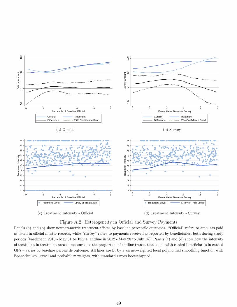
−50

050

100

Offi

cial

Am

ount

0 .2 .4 .6 .8 1Percentile of Baseline Official

Control TreatmentDifference 95% Confidence Band

(a) Official−

500

5010

0S

urve

y A

mou

nt

0 .2 .4 .6 .8 1Percentile of Baseline Survey

Control TreatmentDifference 95% Confidence Band

(b) Survey

0.1

.2.3

.4.5

.6.7

.8.9

1T

reat

men

t Int

ensi

ty

0 .2 .4 .6 .8 1Percentile of Baseline Official

Treatment Level LPoly of Treat Level

(c) Treatment Intensity - Official

0.1

.2.3

.4.5

.6.7

.8.9

1T

reat

men

t Int

ensi

ty

0 .2 .4 .6 .8 1Percentile of Baseline Survey

Treatment Level LPoly of Treat Level

(d) Treatment Intensity - Survey

Figure A.2: Heterogeneity in Official and Survey PaymentsPanels (a) and (b) show nonparametric treatment effects by baseline percentile outcomes. “Official” refers to amounts paid

as listed in official muster records, while “survey” refers to payments received as reported by beneficiaries, both during study

periods (baseline in 2010 - May 31 to July 4; endline in 2012 - May 28 to July 15). Panels (c) and (d) show how the intensity

of treatment in treatment areas – measured as the proportion of endline transactions done with carded beneficiaries in carded

GPs – varies by baseline percentile outcome. All lines are fit by a kernel-weighted local polynomial smoothing function with

Epanechnikov kernel and probability weights, with standard errors bootstrapped.

49

Table A.1: No differential attrition

(a) NREGS

(1)Attriters from

(2)Entrants in

Baseline EndlineControl .024 .086Treatment .013 .061p-value .23 .33

(b) SSP

(1)Attriters from

(2)Entrants in

Baseline EndlineControl .097 .16Treatment .097 .17p-value .99 .41

These tables compare the entire NREGS sample frame – i.e., all jobcard holders – and the entire SSP beneficiary frame across

treatment and control mandals. Column 1 presents the proportion of NREGS jobcards and SSP beneficiaries that dropped

out of the sample frame after baseline, while column 2 presents the proportion that entered the sample frame at endline.

Row 3 reports the p-value of the difference between treatment and control.

Table A.2: Baseline covariates do not predict program implementation

Carded GP Intensity

(1) (2) (3) (4)

Time to Collect (1 hr) -.027 -.011 -.01 -.008(.016) (.014) (.012) (.0099)

Official Amount (Rs. 10,000) -.98 .5 -.016 .93(1.3) (1.3) (1.1) (.98)

Survey Amount (Rs. 10,000) .61 .11 .52 .24(1.5) (1.4) (1.2) (1.1)

Total Income (Rs. 10,000) -.0089 -.01 .00015 -.0042(.0099) (.0077) (.008) (.006)

District FE No Yes No Yes

Adj R-squared 0.01 0.22 -0.00 0.37N. of cases 631 631 631 631

This tables analyzes the effects of baseline covariate variability on endline program implementation in treatment areas.

“Carded GP” is a gram panchayat that has moved to Smartcard based payment, which happens once 40% of beneficiaries

have been issued a card. “Treatment intensity” is the proportion of transactions done with carded beneficiaries in carded

GPs. Standard errors clustered at mandal level in parentheses. Statistical significance is denoted as: ∗p < 0.10, ∗∗p < 0.05,∗∗∗p < 0.01

50

Tab

leA

.3:

Inco

me

incr

ease

s,untr

imm

edsa

mple

(a)

NR

EG

S

Tot

alin

com

eN

RE

GS

Ag

lab

orO

ther

lab

orF

arm

inco

me

Busi

nes

sM

isc

(1)

(2)

(3)

(4)

(5)

(6)

(7)

(8)

Tre

atm

ent

1078

3∗∗

1002

8∗∗

967∗

3630

∗∗45

47∗∗

∗22

33-7

4815

6(4

621)

(461

7)(5

80)

(147

7)(1

645)

(271

6)(1

328)

(240

8)

BL

GP

Mea

n.0

5(.

05)

Dis

tric

tF

EY

esY

esY

esY

esY

esY

esY

esY

es

Adj

R-s

quar

ed0.

030.

030.

010.

040.

020.

010.

010.

01C

ontr

olM

ean

7193

571

935

4743

1478

493

1521

708

6620

1476

5N

.of

case

s49

6749

3349

6649

6749

6749

6749

6749

67

(b)

SS

P

Tot

alin

com

eSSP

Ag

lab

orO

ther

lab

orF

arm

inco

me

Busi

nes

sM

isc

(1)

(2)

(3)

(4)

(5)

(6)

(7)

(8)

Tre

atm

ent

6093

6753

7274

315

18∗

2810

-162

1104

(422

9)(4

252)

(124

)(1

639)

(781

)(2

327)

(104

9)(1

854)

BL

GP

Mea

n.0

39(.

076)

Dis

tric

tF

EY

esY

esY

esY

esY

esY

esY

esY

es

Adj

R-s

quar

ed0.

040.

040.

010.

120.

030.

000.

010.

04C

ontr

olM

ean

5517

155

171

3706

1283

860

4112

434

5626

1453

6N

.of

case

s31

8430

0531

8231

8431

8431

8431

8431

84

Th

ista

ble

anal

yze

sh

ouse

hol

dle

vel

inco

me

for

all

hou

seh

old

s.A

llam

ou

nts

are

inR

up

ees

(Rs.

1=

0.0

18

US

$in

Au

gu

st2012).

“T

ota

lin

com

e”is

full

hou

seh

old

annu

alin

com

ein

2012

from

all

sou

rces

.C

olu

mn

s3-

8b

reak

dow

nth

isfigu

rein

toit

sco

mp

on

ents

.C

olu

mn

3sh

ows

inco

me

from

NR

EG

S(S

SP

inta

ble

(b))

.C

olu

mn

s4

and

5sh

owin

com

efr

omp

hysi

cal

lab

orot

her

than

NR

EG

S,

wit

hco

lum

n4

refe

rrin

gto

inco

me

from

agri

cult

ura

lla

bor

an

dco

lum

n5

inco

me

from

oth

erp

hysi

cal

lab

or.

Col

um

n6

show

sin

com

efr

omfa

rmin

gor

live

stock

,w

hil

eco

lum

n7

show

sb

usi

nes

s/en

trep

ren

euri

al

inco

me.

Colu

mn

8gro

up

sto

get

her

all

oth

erre

main

ing

sou

rces

of

inco

me.

Sta

nd

ard

erro

rscl

ust

ered

atm

and

alle

vel

inp

aren

thes

es.

Sta

tist

ical

sign

ifica

nce

isd

enote

das:∗ p<

0.1

0,∗∗p<

0.05,∗∗∗ p<

0.0

1

51

Table A.4: NREGS earnings: survey and official (scaled)

Official Survey Leakage

(1) (2) (3) (4) (5) (6)

Treatment 9.7 3.8 33 32 -23 -28(25) (24) (21) (20) (21) (20)

BL GP Mean .16∗∗∗ .09∗∗ .14∗∗∗

(.026) (.037) (.031)

District FE Yes Yes Yes Yes Yes Yes

Adj R-squared 0.03 0.05 0.06 0.07 0.06 0.07Control Mean 260 260 180 180 80 80N. of cases 5180 5144 5180 5144 5180 5144

Each observation refers to household-level average weekly amounts for NREGS work done during the study period (baseline

in 2010 - May 31 to July 4; endline in 2012 - May 28 to July 15). The regressions include all sampled beneficiaries who

were a) found by survey team to match official record or b) listed in official records but confirmed as “ghost” beneficiary as

described in Table 5. “Official” refers to amounts paid as listed in official muster records, scaled by the average number of

jobcards per household in the district. “Survey” refers to payments received as reported by beneficiaries. “Leakage” is the

difference between these two amounts. Standard errors clustered at mandal level in parentheses. Statistical significance is

denoted as: ∗p < 0.10, ∗∗p < 0.05, ∗∗∗p < 0.01

52

Tab

leA

.5:

Pro

por

tion

alin

crea

ses

inw

orke

rsat

wor

ksi

teau

dit

s

WSM

Surv

eyO

ffici

alM

ust

er-

WSM

Surv

ey-

WSM

(1)

(2)

(3)

(4)

(5)

(6)

(7)

(8)

(9)

(10)

Tre

atm

ent

1210

6944

2617

146.

857

34(1

2)(1

0)(4

9)(3

6)(2

7)(2

0)(2

0)(1

7)(4

4)(3

5)

Dis

tric

tF

EY

esY

esY

esY

esY

esY

esY

esY

esY

esY

es

Wee

kF

eN

oY

esN

oY

esN

oY

esN

oY

esN

oY

es

Adj

R-s

quar

ed0.

090.

130.

030.

090.

070.

160.

090.

140.

020.

07C

ontr

olM

ean

2828

173

173

108

108

8181

145

145

N.

ofca

ses

513

513

513

513

513

513

513

513

513

513

Un

its

rep

rese

nt

esti

mat

ednu

mb

erof

NR

EG

Sw

orke

rson

agiv

end

ay.

Th

e“W

SM

”nu

mb

ers

are

the

nu

mb

erof

work

ers

fou

nd

inan

ind

epen

den

tau

dit

of

NR

EG

A

wor

ksi

tes

ina

GP

.T

he

“Su

rvey

”va

riab

leis

the

esti

mat

ednu

mb

erof

work

ers

we

exp

ecte

dto

fin

dat

thes

ew

ork

site

sfr

om

hou

seh

old

surv

eyd

ata

when

we

take

into

acco

unt

the

nu

mb

erof

wor

ksi

tes

ina

GP

and

the

aver

age

rep

ort

edw

ork

ing

hou

rsfo

rb

enefi

ciari

es.

“O

ffici

al”

isth

issa

me

esti

mate

for

ad

min

istr

ati

ve

data

.S

tan

dard

erro

rscl

ust

ered

atm

and

alle

vel

inp

aren

thes

es.

Sta

tist

ical

sign

ifica

nce

isd

enote

das:∗ p<

0.1

0,∗∗p<

0.05,∗∗∗ p<

0.0

1

53

Table A.6: No evidence of Hawthorne effects

WSM Official Survey

(1) (2) (3) (4) (5) (6)

HHD Survey in GP -3.4 10 -4.8(8) (34) (33)

WSM in GP 7.5 -13 3 -17 122(31) (28) (42) (37) (106)

WSM Survey in Week -52 -71 -31 -39 38(51) (52) (39) (39) (84)

Recon Survey in Week 12 -.8 45 40 48(69) (68) (52) (51) (90)

District FE Yes Yes Yes Yes Yes Yes

Week Fe Yes Yes Yes Yes Yes Yes

BL GP Value No No Yes No Yes Yes

GP Size FE No Yes Yes No No No

Adj R-squared 0.17Control Mean 48 758 758 755 755 1170Level Week Week Week Week Week WeekSample WSM All All HHD & WSM HHD & WSM HHDN. of cases 682 52311 52311 7728 7728 6153

This table analyzes possible Hawthorne effects from the assorted treatment arms. Each cell represents a separate regression

of the effect on the data source (column) from the survey type (row). Units are number of days worked in a GP per week.

“HHD Survey in GP” is the being surveyed by the household survey. “WSM in GP” is being surveyed by the work site audit.

Control mean represents the area with no survey. “WSM Survey in Week” is whether the work site audit happened in that

specific week. “Recon Survey in week” is whether an enumerator to map the worksites in that specific week. Sample of “All”

refers to all GPs in our study districts. Standard errors clustered at mandal level in parentheses. Statistical significance is

denoted as: ∗p < 0.10, ∗∗p < 0.05, ∗∗∗p < 0.01

54