United States Office of Research and EPA/600/R-01/049 Environmental Protection Development August 2001 Agency Washington, D.C. 20460

Environmental Technology Verification Report

PCB Detection Technology

Dexsil CorporationL2000DX Analyzer

Oak Ridge National Laboratory

THE ENVIRONMENTAL TECHNOLOGY VERIFICATION

Oak Ridge National Laboratory

PROGRAM

Verification Statement

TECHNOLOGY TYPE: ION SPECIFIC ELECTRODE

APPLICATION: MEASUREMENT OF PCBs IN TRANSFORMER OIL

TECHNOLOGY NAME: L2000DX Analyzer

COMPANY: Dexsil Corporation

ADDRESS: One Hamden Park Drive PHONE: (203) 288-3509 Hamden, CT 06517 FAX: (203) 248-6523

WEB SITE: www.dexsil.com E-MAIL: tblynn@dexsil.com

The U.S. Environmental Protection Agency (EPA) has created the Environmental Technology Verification Program (ETV) to facilitate the deployment of innovative or improved environmental technologies through performance verification and dissemination of information. The goal of the ETV Program is to further environmental protection by substantially accelerating the acceptance and use of improved and cost-effective technologies. ETV seeks to achieve this goal by providing high-quality, peer-reviewed data on technology performance to those involved in the design, distribution, financing, permitting, purchase, and use of environmental technologies.

ETV works in partnership with recognized standards and testing organizations and stakeholder groups consisting of regulators, buyers, and vendor organizations, with the full participation of individual technology developers. The program evaluates the performance of innovative technologies by developing test plans that are responsive to the needs of stakeholders, conducting field or laboratory tests (as appropriate), collecting and analyzing data, and preparing peer-reviewed reports. All evaluations are conducted in accordance with rigorous quality assurance protocols to ensure that data of known and adequate quality are generated and that the results are defensible.

Oak Ridge National Laboratory (ORNL) is one of the verification organizations operating under the Site Characterization and Monitoring Technologies (SCMT) program. SCMT, which is administered by EPA’s National Exposure Research Laboratory (NERL), is one of six technology areas under ETV. In this verification test, ORNL evaluated the performance of polychlorinated biphenyl (PCB) detection technologies. This verification statement provides a summary of the test results for Dexsil’s L2000DX instrument.

EPA-VS-SCM-46 The accompanying notice is an integral part of this verification statement. August 2001

VERIFICATION TEST DESCRIPTION

This verification test was designed to evaluate technologies that detect and measure PCBs in transformer oil. The test was conducted at ORNL in Oak Ridge, Tennessee, from August 21 through August 23, 2000. Spiked samples of known concentration were used to assess the accuracy of the technology. Environmentally contaminated oil samples, collected from ORNL transformers and ranging in concentration from 0 to approximately 300 parts per million (ppm), were used to assess several performance characteristics. Tests were conducted outdoors, with naturally fluctuating temperatures and relative humidity conditions. The results of the oil analyses conducted by the technology were compared with results from analyses of homogeneous replicate samples conducted by conventional EPA methodology in an approved reference laboratory. Details of the test, including a data summary and discussion of results, may be found in the report entitled Environmental Technology Verification Report: PCB Detection Technology— Dexsil Corporation, L2000DX, EPA/600/R-01/049.

TECHNOLOGY DESCRIPTION

The L2000DX Analyzer (dimensions: 9 × 9.5 × 4.25 in.) is a field-portable ion-specific electrode instrument, weighing approximately 5 lb 12 oz, designed to quantify concentrations of PCBs, chlorinated solvents, and pesticides in soils, water, transformer oils, and surface wipes. The L2000DX can be operated in the field powered by a rechargeable 8-V gel cell, or in the laboratory using 120-V AC power. To prepare a sample for analysis, 5 mL of the oil is collected in a polyethylene reaction tube. Two glass ampules contained in the reaction tube are broken to introduce metallic sodium to the oil. The mixture is then shaken for 10 s and allowed to react for a total of 1 min. The sodium strips the covalently bonded chlorine atoms off the PCB molecule. An aqueous extraction solution is added to the reaction tube to adjust the pH, destroy the excess sodium, and extract and isolate the newly formed chloride ions in a buffered aqueous solution. The aqueous layer is decanted, filtered, and collected in an analysis vial. The ion-specific electrode is put into this aqueous solution to measure the millivolt potential. The potential is then converted to the equivalent PCB concentration. The lowest concentration reported by the L2000DX is typically 3 ppm. The performance of a previous version of this instrument (the L2000 PCB/Chloride Analyzer) was verified by ETV for soil and solvent extracts in 1998.

VERIFICATION OF PERFORMANCE

The following performance characteristics of the L2000DX were observed:

Precision: Precision—based on the mean percent relative standard deviation—was 11%.

Accuracy: Accuracy was assessed using the nominal concentrations of the spiked oils. The mean percent recovery value for the spiked samples was 112%. The L2000DX results were unbiased for both single -Aroclor and multi-Aroclor mixtures.

False positive/false negative results: Of the 20 blank samples, Dexsil reported PCBs in 5 samples (25% false positives). In addition, false positive and false negative results were determined by comparing the L2000DX results with the reference laboratory results for the environmental and spiked samples. One of the results was reported as a false positive (13% of total), and none were false negatives.

Completeness: The L2000DX generated results for all 152 oil samples, for a completeness of 100%.

EPA-VS-SCM-46 The accompanying notice is an integral part of this verification statement. August 2001

Comparability: A one-to-one sample comparison of the L2000DX results and the reference laboratory results was performed for all samples (spiked and environmental) that were reported as detections. The correlation coefficient (r) for the comparison of the entire oil data set was 0.92 [slope (m) = 0.89]. The reference laboratory’s method was biased high for samples that contained mixtures of overlapping Aroclors (such as a mixture of 1254 and 1260). If the samples containing mixtures of Aroclors are removed from the data set, the r value is 0.95 and the m value is 1.1.

Sample Throughput: Operating in the field, the Dexsil team accomplished a sample throughput rate of approximately eight samples per hour for the oil analyses. One operator prepared the samples, while the other performed the analyses. The instrument can be operated by a single trained analyst.

Overall Evaluation: The overall performance was characterized as unbiased and precise. The verification team found that the L2000DX was relatively simple for the trained analyst to operate in the field, requiring less than an hour for initial setup. As with any technology selection, the user must determine if this technology is appropriate for the application and the project data quality objectives. For more information on this and other verified technologies, visit the ETV web site at http://www.epa.gov/etv.

Gary J. Foley, Ph.D. W. Frank Harris, Ph.D. Director Associate Laboratory Director National Exposure Research Laboratory Biological and Environmental Sciences Office of Research and Development Oak Ridge National Laboratory

NOTICE: EPA verifications are based on evaluations of technology performance under specific, predetermined criteria and appropriate quality assurance procedures. EPA and ORNL make no expressed or implied warranties as to the performance of the technology and do not certify that a technology will always operate as verified. The end user is solely responsible for complying with any and all applicable federal, state, and local requirements. Mention of commercial product names does not imply endorsement or recommendation.

EPA-VS-SCM-46 The accompanying notice is an integral part of this verification statement. August 2001

EPA/600/R-01/049 August 2001

Environmental Technology Verification Report

PCB Detection Technology

Dexsil CorporationL2000DX Analyzer

By

Amy B. DindalCharles K. Bayne, Ph.D.Roger A. Jenkins, Ph.D.

Oak Ridge National LaboratoryOak Ridge, Tennessee 37831-6120

Eric N. KoglinU.S. Environmental Protection Agency

Environmental Sciences Division National Exposure Research Laboratory

Las Vegas, Nevada 89193-3478

Notice

The U.S. Environmental Protection Agency (EPA), through its Office of Research and Development (ORD), funded and managed, through Interagency Agreement No. DW89937854 with Oak Ridge National Laboratory, the verification effort described herein. This report has been peer and administratively reviewed and has been approved for publication as an EPA document. Mention of trade names or commercial products does not constitute endorsement or recommendation for use of a specific product.

ii

Table of Contents

List of Figures . . . . . . . . . . . . . . . . . . . . . . . . . . . . . . . . . . . . . . . . . . . . . . . . . . . . . . . . . . . . . . . . . . . . . . v List of Tables . . . . . . . . . . . . . . . . . . . . . . . . . . . . . . . . . . . . . . . . . . . . . . . . . . . . . . . . . . . . . . . . . . . . . . . vii Acknowledgments . . . . . . . . . . . . . . . . . . . . . . . . . . . . . . . . . . . . . . . . . . . . . . . . . . . . . . . . . . . . . . . . . . . ix Abbreviations and Acronyms . . . . . . . . . . . . . . . . . . . . . . . . . . . . . . . . . . . . . . . . . . . . . . . . . . . . . . . . . . xi

1. INTRODUCTION . . . . . . . . . . . . . . . . . . . . . . . . . . . . . . . . . . . . . . . . . . . . . . . . . . . . . . . . . . . . . . . . 1

2. TECHNOLOGY DESCRIPTION . . . . . . . . . . . . . . . . . . . . . . . . . . . . . . . . . . . . . . . . . . . . . . . . . . . . 2 General Technology Description . . . . . . . . . . . . . . . . . . . . . . . . . . . . . . . . . . . . . . . . . . . . . . . . . . . . 2 Oil Sample Preparation . . . . . . . . . . . . . . . . . . . . . . . . . . . . . . . . . . . . . . . . . . . . . . . . . . . . . . . . . . . . 2 Instrument Calibration . . . . . . . . . . . . . . . . . . . . . . . . . . . . . . . . . . . . . . . . . . . . . . . . . . . . . . . . . . . . . 2 Sample Analysis . . . . . . . . . . . . . . . . . . . . . . . . . . . . . . . . . . . . . . . . . . . . . . . . . . . . . . . . . . . . . . . . . 2

3. VERIFICATION TEST DESIGN . . . . . . . . . . . . . . . . . . . . . . . . . . . . . . . . . . . . . . . . . . . . . . . . . . . . 4 Objective . . . . . . . . . . . . . . . . . . . . . . . . . . . . . . . . . . . . . . . . . . . . . . . . . . . . . . . . . . . . . . . . . . . . . . . 4 Testing Location and Conditions . . . . . . . . . . . . . . . . . . . . . . . . . . . . . . . . . . . . . . . . . . . . . . . . . . . . 4 Sample Descriptions . . . . . . . . . . . . . . . . . . . . . . . . . . . . . . . . . . . . . . . . . . . . . . . . . . . . . . . . . . . . . . 4

ORNL Transformer Oil Samples . . . . . . . . . . . . . . . . . . . . . . . . . . . . . . . . . . . . . . . . . . . . . . . . . 4 Quality Control Samples . . . . . . . . . . . . . . . . . . . . . . . . . . . . . . . . . . . . . . . . . . . . . . . . . . . . . . . . 4

Sample Randomization . . . . . . . . . . . . . . . . . . . . . . . . . . . . . . . . . . . . . . . . . . . . . . . . . . . . . . . . . . . . 5 Summary of Experimental Design . . . . . . . . . . . . . . . . . . . . . . . . . . . . . . . . . . . . . . . . . . . . . . . . . . . 5 Description of Performance Factors . . . . . . . . . . . . . . . . . . . . . . . . . . . . . . . . . . . . . . . . . . . . . . . . . . 6

Precision . . . . . . . . . . . . . . . . . . . . . . . . . . . . . . . . . . . . . . . . . . . . . . . . . . . . . . . . . . . . . . . . . . . . 6 Accuracy . . . . . . . . . . . . . . . . . . . . . . . . . . . . . . . . . . . . . . . . . . . . . . . . . . . . . . . . . . . . . . . . . . . . 6 False Positive/Negative Results . . . . . . . . . . . . . . . . . . . . . . . . . . . . . . . . . . . . . . . . . . . . . . . . . . 6 Completeness . . . . . . . . . . . . . . . . . . . . . . . . . . . . . . . . . . . . . . . . . . . . . . . . . . . . . . . . . . . . . . . . 6 Comparability . . . . . . . . . . . . . . . . . . . . . . . . . . . . . . . . . . . . . . . . . . . . . . . . . . . . . . . . . . . . . . . . 6 Sample Throughput . . . . . . . . . . . . . . . . . . . . . . . . . . . . . . . . . . . . . . . . . . . . . . . . . . . . . . . . . . . . 7 Ease of Use . . . . . . . . . . . . . . . . . . . . . . . . . . . . . . . . . . . . . . . . . . . . . . . . . . . . . . . . . . . . . . . . . . 7 Cost . . . . . . . . . . . . . . . . . . . . . . . . . . . . . . . . . . . . . . . . . . . . . . . . . . . . . . . . . . . . . . . . . . . . . . . . 7 Miscellaneous Factors . . . . . . . . . . . . . . . . . . . . . . . . . . . . . . . . . . . . . . . . . . . . . . . . . . . . . . . . . 7

4. REFERENCE LABORATORY ANALYSES . . . . . . . . . . . . . . . . . . . . . . . . . . . . . . . . . . . . . . . . . . 8 Background . . . . . . . . . . . . . . . . . . . . . . . . . . . . . . . . . . . . . . . . . . . . . . . . . . . . . . . . . . . . . . . . . . . . . 8 Reference Laboratory Selection . . . . . . . . . . . . . . . . . . . . . . . . . . . . . . . . . . . . . . . . . . . . . . . . . . . . . 8 Reference Laboratory Method . . . . . . . . . . . . . . . . . . . . . . . . . . . . . . . . . . . . . . . . . . . . . . . . . . . . . . 9 Reference Laboratory Performance . . . . . . . . . . . . . . . . . . . . . . . . . . . . . . . . . . . . . . . . . . . . . . . . . . . 9

5. TECHNOLOGY EVALUATION . . . . . . . . . . . . . . . . . . . . . . . . . . . . . . . . . . . . . . . . . . . . . . . . . . . . 11 Objective and Approach . . . . . . . . . . . . . . . . . . . . . . . . . . . . . . . . . . . . . . . . . . . . . . . . . . . . . . . . . . . 11 Precision . . . . . . . . . . . . . . . . . . . . . . . . . . . . . . . . . . . . . . . . . . . . . . . . . . . . . . . . . . . . . . . . . . . . . . . 11 Accuracy . . . . . . . . . . . . . . . . . . . . . . . . . . . . . . . . . . . . . . . . . . . . . . . . . . . . . . . . . . . . . . . . . . . . . . . 11 False Positive/False Negative Results . . . . . . . . . . . . . . . . . . . . . . . . . . . . . . . . . . . . . . . . . . . . . . . . . 11 Completeness . . . . . . . . . . . . . . . . . . . . . . . . . . . . . . . . . . . . . . . . . . . . . . . . . . . . . . . . . . . . . . . . . . . . 11 Comparability . . . . . . . . . . . . . . . . . . . . . . . . . . . . . . . . . . . . . . . . . . . . . . . . . . . . . . . . . . . . . . . . . . . 11 Sample Throughput . . . . . . . . . . . . . . . . . . . . . . . . . . . . . . . . . . . . . . . . . . . . . . . . . . . . . . . . . . . . . . . 13 Ease of Use . . . . . . . . . . . . . . . . . . . . . . . . . . . . . . . . . . . . . . . . . . . . . . . . . . . . . . . . . . . . . . . . . . . . . 13

iii

Cost Assessment . . . . . . . . . . . . . . . . . . . . . . . . . . . . . . . . . . . . . . . . . . . . . . . . . . . . . . . . . . . . . . . . . 13 L2000DX Costs . . . . . . . . . . . . . . . . . . . . . . . . . . . . . . . . . . . . . . . . . . . . . . . . . . . . . . . . . . . . . . 15

Labor . . . . . . . . . . . . . . . . . . . . . . . . . . . . . . . . . . . . . . . . . . . . . . . . . . . . . . . . . . . . . . . . . . . 15 Equipment . . . . . . . . . . . . . . . . . . . . . . . . . . . . . . . . . . . . . . . . . . . . . . . . . . . . . . . . . . . . . . . 16

Reference Laboratory Costs . . . . . . . . . . . . . . . . . . . . . . . . . . . . . . . . . . . . . . . . . . . . . . . . . . . . . 16 Sample Shipment . . . . . . . . . . . . . . . . . . . . . . . . . . . . . . . . . . . . . . . . . . . . . . . . . . . . . . . . . . 16 Labor, Equipment, and Waste Disposal . . . . . . . . . . . . . . . . . . . . . . . . . . . . . . . . . . . . . . . . . 16

Cost Assessment Summary . . . . . . . . . . . . . . . . . . . . . . . . . . . . . . . . . . . . . . . . . . . . . . . . . . . . . . 17 Miscellaneous Factors . . . . . . . . . . . . . . . . . . . . . . . . . . . . . . . . . . . . . . . . . . . . . . . . . . . . . . . . . . . . . 17 Summary of Performance . . . . . . . . . . . . . . . . . . . . . . . . . . . . . . . . . . . . . . . . . . . . . . . . . . . . . . . . . . 17

6. REFERENCES . . . . . . . . . . . . . . . . . . . . . . . . . . . . . . . . . . . . . . . . . . . . . . . . . . . . . . . . . . . . . . . . . . 19

Appendix A — Dexsil’s L2000DX Results Compared with Reference Laboratory Results . . . . . . . . . . . . . . . . . . . . . . . . . . . . . . . . . . . . . . . . . . . . . . . . . . . . . . . . . . . . . . . 21

Appendix B — Data Quality Objective (DQO) Example . . . . . . . . . . . . . . . . . . . . . . . . . . . . . . . . . . . . . 25

iv

List of Figures

1 L2000DX Analyzer . . . . . . . . . . . . . . . . . . . . . . . . . . . . . . . . . . . . . . . . . . . . . . . . . . . . . . . . . . . . 2 2 L2000DX PCB results versus reference laboratory results for all samples . . . . . . . . . . . . . . . . . 14 3 L2000DX PCB results versus reference laboratory results, excluding samples

containing mixtures of Aroclors . . . . . . . . . . . . . . . . . . . . . . . . . . . . . . . . . . . . . . . . . . . . . . . . . . 14 4 Range of percent difference (%D) values for PCB results . . . . . . . . . . . . . . . . . . . . . . . . . . . . . . 15

v

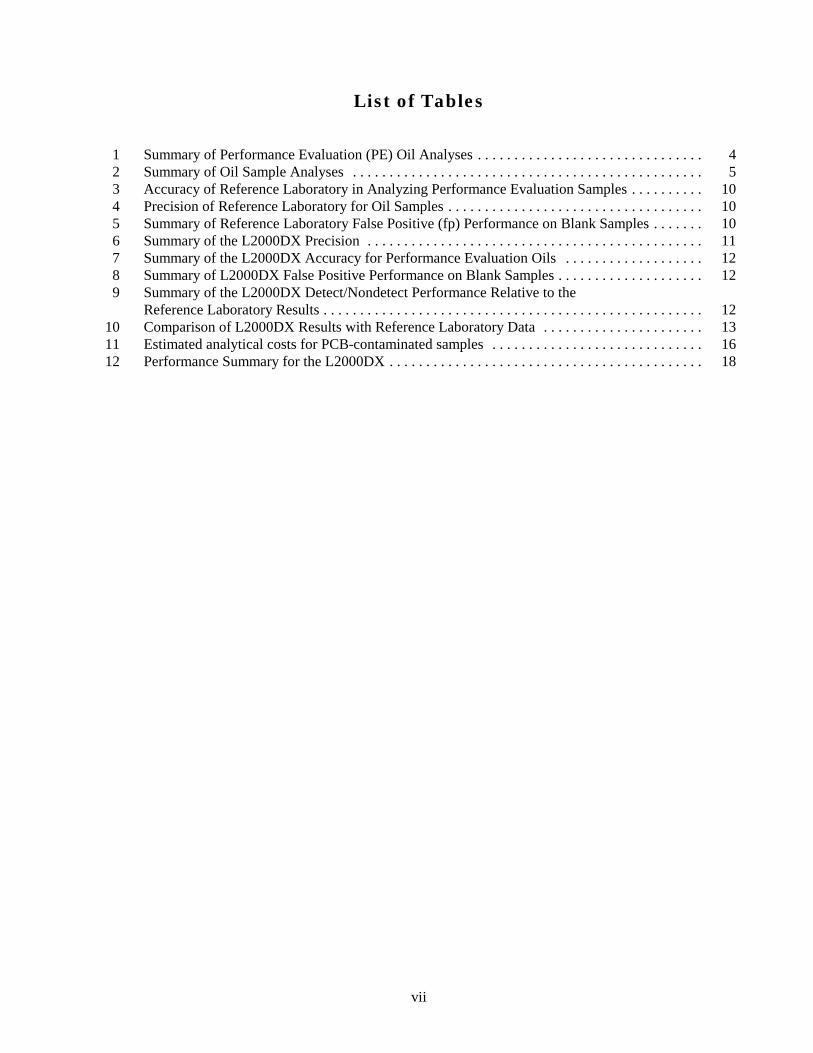
List of Tables

1 Summary of Performance Evaluation (PE) Oil Analyses . . . . . . . . . . . . . . . . . . . . . . . . . . . . . . . 4 2 Summary of Oil Sample Analyses . . . . . . . . . . . . . . . . . . . . . . . . . . . . . . . . . . . . . . . . . . . . . . . . 5 3 Accuracy of Reference Laboratory in Analyzing Performance Evaluation Samples . . . . . . . . . . 10 4 Precision of Reference Laboratory for Oil Samples . . . . . . . . . . . . . . . . . . . . . . . . . . . . . . . . . . . 10 5 Summary of Reference Laboratory False Positive (fp) Performance on Blank Samples . . . . . . . 10 6 Summary of the L2000DX Precision . . . . . . . . . . . . . . . . . . . . . . . . . . . . . . . . . . . . . . . . . . . . . . 11 7 Summary of the L2000DX Accuracy for Performance Evaluation Oils . . . . . . . . . . . . . . . . . . . 12 8 Summary of L2000DX False Positive Performance on Blank Samples . . . . . . . . . . . . . . . . . . . . 12 9 Summary of the L2000DX Detect/Nondetect Performance Relative to the

Reference Laboratory Results . . . . . . . . . . . . . . . . . . . . . . . . . . . . . . . . . . . . . . . . . . . . . . . . . . . . 12 10 Comparison of L2000DX Results with Reference Laboratory Data . . . . . . . . . . . . . . . . . . . . . . 13 11 Estimated analytical costs for PCB-contaminated samples . . . . . . . . . . . . . . . . . . . . . . . . . . . . . 16 12 Performance Summary for the L2000DX . . . . . . . . . . . . . . . . . . . . . . . . . . . . . . . . . . . . . . . . . . . 18

vii

Acknowledgments

The authors wish to acknowledge the support of all those who helped plan and conduct the verification test, analyze the data, and prepare this report. In particular, we recognize the technical expertise of Viorica Lopez-Avila (Midwest Research Institute), who was the peer reviewer of this report. For sample collection support, we thank Kevin Norris, Charlie Bruce, and Fred Morgeson (Oak Ridge National Laboratory). The authors also acknowledge the participation of Dexsil Corporation, in particular, Ted Lynn and Dave Balog, who performed the analyses during the test.

For more information on the PCB Detection Technology Verification contact

Eric N. Koglin Roger A. Jenkins Project Technical Leader Program Manager Environmental Protection Agency Oak Ridge National Laboratory Environmental Sciences Division Chemical and Analytical Sciences Division National Exposure Research Laboratory P.O. Box 2008 P.O. Box 93478 Oak Ridge, TN 37831-6120 Las Vegas, Nevada 89193-3478 (865) 574-4871 (702) 798-2432 jenkinsra@ornl.gov koglin.eric@epa.gov

For more information on Dexsil’s L2000DX Analyzer contact

Ted Lynn Dexsil Corporation One Hamden Park Drive Hamden, CT 06517 (203) 288-3509 tblynn@dexsil.com www.dexsil.com

ix

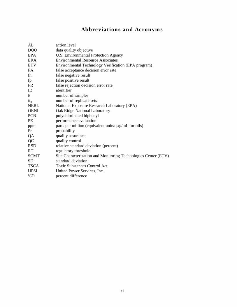
Abbreviations and Acronyms

AL action level DQO data quality objective EPA U.S. Environmental Protection Agency ERA Environmental Resource Associates ETV Environmental Technology Verification (EPA program) FA false acceptance decision error rate fn false negative result fp false positive result FR false rejection decision error rate ID identifier N number of samples NR number of replicate sets NERL National Exposure Research Laboratory (EPA) ORNL Oak Ridge National Laboratory PCB polychlorinated biphenyl PE performance evaluation ppm parts per million (equivalent units: �g/mL for oils) Pr probability QA quality assurance QC quality control RSD relative standard deviation (percent) RT regulatory threshold SCMT Site Characterization and Monitoring Technologies Center (ETV) SD standard deviation TSCA Toxic Substances Control Act UPSI United Power Services, Inc. %D percent difference

xi

Section 1 — Introduction

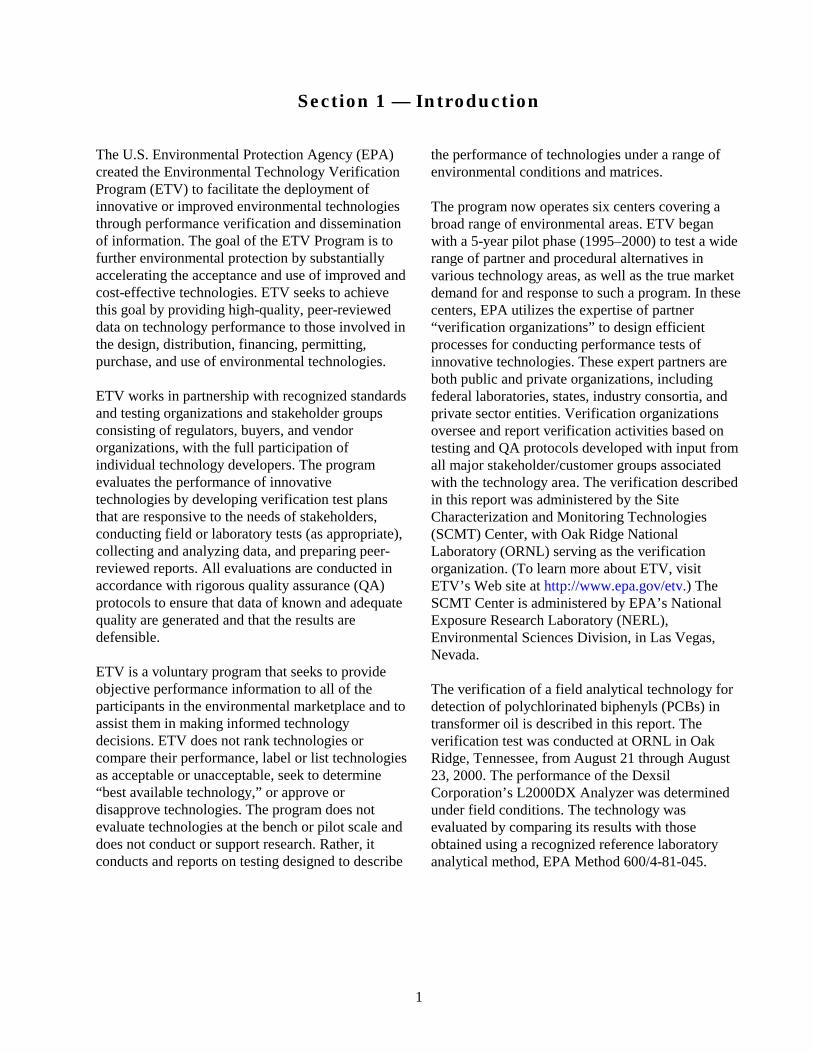
The U.S. Environmental Protection Agency (EPA) created the Environmental Technology Verification Program (ETV) to facilitate the deployment of innovative or improved environmental technologies through performance verification and dissemination of information. The goal of the ETV Program is to further environmental protection by substantially accelerating the acceptance and use of improved and cost-effective technologies. ETV seeks to achieve this goal by providing high-quality, peer-reviewed data on technology performance to those involved in the design, distribution, financing, permitting, purchase, and use of environmental technologies.

ETV works in partnership with recognized standards and testing organizations and stakeholder groups consisting of regulators, buyers, and vendor organizations, with the full participation of individual technology developers. The program evaluates the performance of innovative technologies by developing verification test plans that are responsive to the needs of stakeholders, conducting field or laboratory tests (as appropriate), collecting and analyzing data, and preparing peer­reviewed reports. All evaluations are conducted in accordance with rigorous quality assurance (QA) protocols to ensure that data of known and adequate quality are generated and that the results are defensible.

ETV is a voluntary program that seeks to provide objective performance information to all of the participants in the environmental marketplace and to assist them in making informed technology decisions. ETV does not rank technologies or compare their performance, label or list technologies as acceptable or unacceptable, seek to determine “best available technology,” or approve or disapprove technologies. The program does not evaluate technologies at the bench or pilot scale and does not conduct or support research. Rather, it conducts and reports on testing designed to describe

the performance of technologies under a range of environmental conditions and matrices.

The program now operates six centers covering a broad range of environmental areas. ETV began with a 5-year pilot phase (1995–2000) to test a wide range of partner and procedural alternatives in various technology areas, as well as the true market demand for and response to such a program. In these centers, EPA utilizes the expertise of partner “verification organizations” to design efficient processes for conducting performance tests of innovative technologies. These expert partners are both public and private organizations, including federal laboratories, states, industry consortia, and private sector entities. Verification organizations oversee and report verification activities based on testing and QA protocols developed with input from all major stakeholder/customer groups associated with the technology area. The verification described in this report was administered by the Site Characterization and Monitoring Technologies (SCMT) Center, with Oak Ridge National Laboratory (ORNL) serving as the verification organization. (To learn more about ETV, visit ETV’s Web site at http://www.epa.gov/etv.) The SCMT Center is administered by EPA’s National Exposure Research Laboratory (NERL), Environmental Sciences Division, in Las Vegas, Nevada.

The verification of a field analytical technology for detection of polychlorinated biphenyls (PCBs) in transformer oil is described in this report. The verification test was conducted at ORNL in Oak Ridge, Tennessee, from August 21 through August 23, 2000. The performance of the Dexsil Corporation’s L2000DX Analyzer was determined under field conditions. The technology was evaluated by comparing its results with those obtained using a recognized reference laboratory analytical method, EPA Method 600/4-81-045.

1

Section 2 — Technology Description

In this section, the vendor (with minimal editorial changes by ORNL) provides a description of the technology and the analytical procedure used during the verification testing activities.

General Technology Description The L2000DX Analyzer (dimensions: 9 × 9.5 × 4.25 in.; see Figure 1) is a field-portable ion­specific electrode instrument, weighing approximately 5 lb 12 oz, designed to quantify concentrations of PCBs, chlorinated solvents, and pesticides in soils, water, transformer oils, and surface wipes. The L2000DX can be operated in the field powered by a rechargeable 8-V gel cell, or in the laboratory using 120-V AC power. In this verification test, the lowest reported concentration of PCBs in transformer oil was 3 ppm. The performance of a previous version of this instrument (the L2000 PCB/Chloride Analyzer) was verified by ETV for soil and solvent extracts in 1998 (EPA 1998).

Oil Sample Preparation Sample preparation begins by collecting 5 mL of the oil in a polyethylene reaction tube. Two glass ampules contained in the reaction tube are broken, introducing metallic sodium to the oil. The mixture is then shaken for 10 s and allowed to react for a total of 1 min. The sodium strips the covalently bonded chlorine atoms off the PCB molecule. An aqueous extraction solution is added

to the reaction tube to adjust the pH, destroy the excess sodium, and extract and isolate the newly formed chloride ions in a buffered aqueous solution. The aqueous layer is decanted, filtered, and collected in an analysis vial. The ion-specific electrode is put into this aqueous solution to measure the millivolt potential. The potential is then converted to the equivalent PCB concentration.

Instrument Calibration A one-point calibration is performed prior to sample analysis. The analyst simply follows the menu-driven instructions prompted in the display. When prompted, the instrument will ask if the calibration solution is ready. The analyst inserts the ion-specific electrode into the 50-ppm chloride solution and then pushes the “yes” button. The instrument will then prompt the user when the calibration is completed. Additional calibration is required when the instrument prompts the user, approximately every 15 min.

Sample Analysis To begin analysis of the sample, the analyst chooses the appropriate Aroclor from the

Figure 1. L2000DX Analyzer.

2

programmed menu. If the Aroclor is not known or “enter” button. After approximately 30 s, the PCB if there is a mixture of Aroclors, Aroclor 1242 concentration of the samples (in ppm) is displayed should be chosen for the most conservative by the L2000DX. results. The analyst then places the electrode into the aqueous extract solution and pushes the

3

Section 3 — Verification Test Design

Objective The purpose of this section is to describe the verification test design. It is a summary of the test plan (ORNL 2000).

Testing Location and Conditions The verification of field analytical technologies for PCBs was conducted on the grounds outside of ORNL’s Building 5507, in Oak Ridge, Tennessee. The temperature and relative humidity were monitored during field testing. Over the three days of testing, the average temperature was 84ºF, and temperatures ranged from 63 to 98ºF. The average relative humidity was 55%, and relative humidity ranged from 27 to 90%.

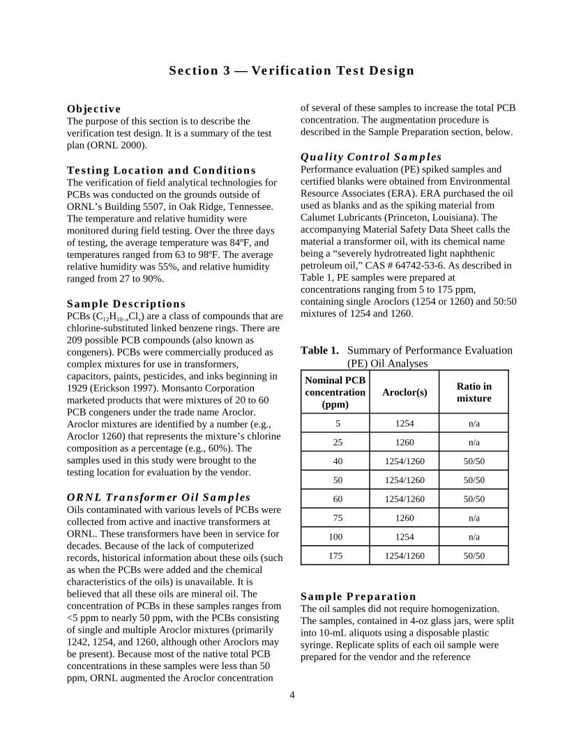
Sample Descriptions PCBs (C12H10–xClx) are a class of compounds that are chlorine-substituted linked benzene rings. There are 209 possible PCB compounds (also known as congeners). PCBs were commercially produced as complex mixtures for use in transformers, capacitors, paints, pesticides, and inks beginning in 1929 (Erickson 1997). Monsanto Corporation marketed products that were mixtures of 20 to 60 PCB congeners under the trade name Aroclor. Aroclor mixtures are identified by a number (e.g., Aroclor 1260) that represents the mixture’s chlorine composition as a percentage (e.g., 60%). The samples used in this study were brought to the testing location for evaluation by the vendor.

ORNL Transformer Oil Samples Oils contaminated with various levels of PCBs were collected from active and inactive transformers at ORNL. These transformers have been in service for decades. Because of the lack of computerized records, historical information about these oils (such as when the PCBs were added and the chemical characteristics of the oils) is unavailable. It is believed that all these oils are mineral oil. The concentration of PCBs in these samples ranges from <5 ppm to nearly 50 ppm, with the PCBs consisting of single and multiple Aroclor mixtures (primarily 1242, 1254, and 1260, although other Aroclors may be present). Because most of the native total PCB concentrations in these samples were less than 50 ppm, ORNL augmented the Aroclor concentration

of several of these samples to increase the total PCB concentration. The augmentation procedure is described in the Sample Preparation section, below.

Quality Control Samples Performance evaluation (PE) spiked samples and certified blanks were obtained from Environmental Resource Associates (ERA). ERA purchased the oil used as blanks and as the spiking material from Calumet Lubricants (Princeton, Louisiana). The accompanying Material Safety Data Sheet calls the material a transformer oil, with its chemical name being a “severely hydrotreated light naphthenic petroleum oil,” CAS # 64742-53-6. As described in Table 1, PE samples were prepared at concentrations ranging from 5 to 175 ppm, containing single Aroclors (1254 or 1260) and 50:50 mixtures of 1254 and 1260.

Table 1. Summary of Performance Evaluation (PE) Oil Analyses

Nominal PCB concentration

(ppm) Aroclor(s)

Ratio in mixture

5 1254 n/a

25 1260 n/a

40 1254/1260 50/50

50 1254/1260 50/50

60 1254/1260 50/50

75 1260 n/a

100 1254 n/a

175 1254/1260 50/50

Sample Preparation The oil samples did not require homogenization. The samples, contained in 4-oz glass jars, were split into 10-mL aliquots using a disposable plastic syringe. Replicate splits of each oil sample were prepared for the vendor and the reference

4

laboratory. Three sets of archives were also prepared.

As mentioned previously, the ORNL transformer oil samples originally contained PCB concentrations of <50 ppm. Several of the transformer oils were aug­mented with additional Aroclors (up to ~200 ppm), so that a larger dynamic range could be tested. To spike the samples, ~250 mL of oil was poured into a 1-L wide-mouth jar. A stir bar was added; then the jar was placed on a magnetic stirrer. While the oil was being stirred, hexane solutions with known concentrations of Aroclors were added to increase the total PCB concentration. One Aroclor was added to each augmented transformer oil. Typically, the Aroclor already present in the sample was the one that was added. For example, if the native PCB concentration was 3 ppm of Aroclor 1260, then 50 ppm of Aroclor 1260 was added to the oil.

The concentrations of all samples used in the study were confirmed by an ORNL in-house method. The oil samples were prepared by diluting 1 g of oil in 10 mL of hexane. The hexane extract was analyzed on a Hewlett Packard 6890 gas chromatograph equipped with an electron capture detector and an autosampler. The analytical method used was a slightly modified version of EPA’s SW-846 dual­column Method 8081 (EPA 1994).

Sample Randomization The samples were randomized in two stages. First, the order in which the filled jars were distributed was randomized so that the vendor did not always receive the first jar filled for a given sample set. Second, the order of analysis was randomized so that Dexsil and the reference laboratory analyzed the same set of samples, but in a different order. Each jar was labeled with a sample number. Replicate samples were assigned unique (but not sequential) sample numbers. Spiked materials and blanks were labeled in the same manner, such that these quality control (QC) samples were indistinguishable from other samples. All samples were analyzed blindly by both the vendor and the reference laboratory.

Summary of Experimental Design The distribution of samples is shown in Table 2. A total of 152 oil samples were analyzed, with approximately 65% of the samples being naturally contaminated and augmented transformer oils, and the remaining 35% being PE samples and blanks. Four replicates were analyzed for each sample type. For example, four environmental samples were analyzed in the 50.1- to 75.0-ppm concentration range, indicating that 16 individual samples were used in the study.

Table 2. Summary of Oil Sample Analyses

Target concentration range Number of samples a

(ppm) Environmental PE

Blank 2 5

�5.0 2 1

5.1–25.0 4 1

25.1–40.0 4 1

40.1–50.0 3 1

50.1–75.0 4 2

75.1–100.0 2 1

> 100 4 1

All samples, incl. 4 replicates each 100 52 a Four replicates were analyzed for each sample.

5

Description of Performance Factors In Section 5, technology performance is described in terms of precision, accuracy, completeness, and comparability, which are indicators of data quality (EPA 1996). False positive and negative results, sample throughput, and ease of use are also described. Each of these performance characteristics is defined in this section.

Precision Precision is the reproducibility of measurements under a given set of conditions. Standard deviation (SD) and relative standard deviation (RSD) for replicate results are used to assess precision, using the following equation:

RSD = (SD/average concentration) × 100% . (Eq. 1)

The overall RSD is characterized by three summary values:

• mean — i.e., average; • median — i.e., 50th percentile value, at which

50% of all individual RSD values are below and 50% are above; and

• range — i.e., the highest and lowest RSD values that were reported.

The average RSD may not be the best representation of precision, but it is reported for convenient reference. RSDs greater than 100% should be viewed as indicators of large variability and possibly non-normal distributions.

Accuracy Accuracy represents the closeness of the tech­nology’s measured concentrations to known (in this case, spiked/PE) values. Accuracy is assessed in terms of percent recovery, calculated by the following equation:

% recovery = (measured concentration/ known concentration) × 100% .

(Eq. 2)

As with precision, the overall percent recovery is characterized by three summary values: mean, median, and range.

False Positive/Negative Results A false positive (fp) result is one in which the technology detects PCBs in the sample when there actually are none (Berger, McCarty, and Smith 1996). A false negative (fn) result is one in which the technology indicates that no PCBs are present in the sample when there actually are (Berger, McCarty, and Smith 1996). The evaluation of fp and fn results is influenced by the actual concentration in the sample and includes an assessment of the reporting limits of the technology.

False positive results are assessed in two ways. First, the results are assessed relative to the blanks (i.e., the technology reports a detected value when the sample is a blank). Second, the results are assessed on environmental and spiked samples where the analyte was not detected by the reference laboratory (i.e., the reference laboratory reports a nondetect and the field technology reports a detection).

False negative results, also assessed for environmental and spiked samples, indicate the frequency with which the technology reported a nondetect (i.e., less than reporting limits) and the reference laboratory reported a detection.

The reference laboratory results were validated by ORNL so that fp/fn assessment would not be influenced by faulty laboratory data. The reporting limit is considered in the evaluation. For example, if the reference laboratory reported a result as 0.9 ppm, and the technology’s paired result was reported as below reporting limits (<1 ppm), the technology’s result was considered correct and not a false negative result.

Completeness Completeness is defined as the percentage of measurements that are judged to be usable (i.e., the result is not rejected). The acceptable completeness is 95% or greater.

Comparability Comparability refers to how well the field technology and reference laboratory data agree. The difference between accuracy and comparability is that accuracy is judged relative to a known value, and comparability is judged relative to the results of a standard or reference procedure, which may or may not report the results accurately. The reference

6

laboratory result is not assumed to be the “correct” result. This evaluation is performed to compare the result from the field analytical technology with what a typical fixed analytical laboratory might report for the same sample. A one-to-one sample comparison of the technology results and the reference laboratory results is performed in Section 5.

A correlation coefficient quantifies the linear relationship between two measurements (Draper and Smith 1981). The correlation coefficient is denoted by the letter r; its value ranges from –1 to +1, where 0 indicates the absence of any linear relationship. The value r = –1 indicates a perfect negative linear relation (one measurement decreases as the second measurement increases); the value r = +1 indicates a perfect positive linear relation (one measurement increases as the second measurement increases).

The slope of the linear regression line, denoted by the letter m, is related to r. Whereas r represents the linear association between the vendor and reference laboratory concentrations, m quantifies the amount of change in the vendor’s measurements relative to the reference laboratory’s measurements. A value of +1 for the slope indicates perfect agreement. (It should be noted that the intercept of the line must be close to zero [i.e., not statistically different from zero], in order for the slope value of +1 to indicate perfect agreement.) Values greater than 1 indicate that the vendor results are generally higher than those of the reference laboratory, while values less than 1 indicate that the vendor results are usually lower than the values from the reference laboratory.

In addition, a direct comparison between the field technology and reference laboratory data is performed by evaluating the percent difference (%D) between the measured concentrations, defined as

%D = ([field technology] – [ref lab])/(ref lab) × 100% . (Eq. 3)

The range of %D values is summarized and reported in Section 5.

Sample Throughput Sample throughput is a measure of the number of samples that can be processed and reported by a technology in a given period of time. This is reported in Section 5 as number of samples per hour or day times the number of analysts.

Ease of Use A significant decision factor in purchasing an instrument or a test kit is how easy the technology is to use. Several factors are evaluated and reported on in Section 5:

• What is the required operator skill level (e.g., technician or advanced degree)?

• How many operators were used during the test? Could the technology be run by a single person?

• How much training would be required in order to run this technology?

• How much subjective decision-making is required?

Cost An important factor in the consideration of whether to purchase a technology is cost. Costs involved with operating the technology and the standard reference analyses are estimated in Section 5. To account for the variability in cost data and assumptions, the economic analysis is presented as a list of cost elements and a range of costs for sample analysis. Several factors affect the cost of analysis. Where possible, these factors are addressed so that decision makers can independently complete a site­specific economic analysis to suit their needs.

Miscellaneous Factors Any other information that might be useful to a person who is considering purchasing the technology is documented in Section 5. Examples of information that might be useful to a prospective purchaser are the amount of hazardous waste generated during the analyses, the ruggedness of the technology, the amount of electrical or battery power necessary to operate the technology, and aspects of the technology or method that make it user-friendly or user-unfriendly.

7

Section 4 — Reference Laboratory Analyses

Background The verification process is based on the presence of a statistically validated data set against which the performance of the technology may be compared. The choice of an appropriate reference method and reference laboratory are critical to the success of the verification test. To assess the performance of the PCB field analytical technology, the data obtained from the verification test participant were compared to data obtained using a conventional analytical method.

Verifications of technologies for the detection and quantification of PCBs in soil and solvent extracts occurred under the ETV program in 1997, 1998, and 2000. EPA SW-846 Method 8081 (EPA 1994) was the reference method used for these verifications. Since the time of the original PCB analyses, Method 8081 has been updated to Method 8082 for PCB analyses. When planning for the verification test of the L2000DX Analyzer to detect PCBs in transformer oils, we considered using Method 8082 to generate the reference results. Further investigation into reference methods indicated that the test method outlined in EPA 600/4-81-045, The Determination of Polychlorinated Biphenyls in Transformer Fluid and Waste Oils (EPA 1982) was more appropriate, as this is the method that is frequently used by the utilities industry.

The fundamental difference between Methods 8082 and 600 is based on the quantification of the total PCB concentration. In Method 8082, Aroclor quantifications are typically performed by selecting three to five representative peaks, confirming that the peaks are within the established retention time windows, integrating the selected peaks, quantifying the peaks based on the calibrations, and averaging the results to obtain a single concentration value for the multi-component Aroclor. If mixtures of Aroclors are suspected to be present, the sample is typically quantified as the most representative Aroclor pattern. If the identification of multiple Aroclors is definitive, total PCBs in the sample are calculated by summing the concentrations of all Aroclors.

In Method 600, more peaks (typically five to ten) are selected as representative for each Aroclor. For quantification, the total area of these peaks is compared to the total area curve generated from the calibration standards. When mixtures of Aroclors are present, typically all Aroclors are quantified and summed to indicate a total PCB concentration.

A direct comparison by ORNL of data generated by Method 8082 and by Method 600 on 36 split oil samples indicated that the two methods usually yielded comparable results for single Aroclor oils, but that Method 600 usually generated a higher PCB value for samples with overlapping mixtures of Aroclors.

Reference Laboratory Selection United Power Services, Inc. (UPSI), of Nashville, Tennessee, was selected to perform the reference analyses. Part of the selection process involved a predemonstration study in which 40 oil samples were sent to UPSI for blind analysis. Included in the design were replicates, blanks, spikes, and actual transformer oil samples. Results from this study indicated that UPSI was proficient in analyzing oils for PCBs.

ORNL performed an on-site audit of UPSI on September 8, 2000, during the UPSI analysis of the verification samples. The purpose of the visit was to observe laboratory operations while ETV oil samples were being analyzed to verify that UPSI maintained the level of QC needed for reference data. UPSI is a small laboratory with one analyst dedicated to the analysis of PCBs in oil. UPSI analyzed approximately 19,000 oils for PCBs in 1999. In addition, the company has an extremely quick turnaround time (2–3 weeks) and competitive prices ($10–20 per sample). Based on observations and interviews during the visit, ORNL staff concluded that the analyst appeared to be very meticulous and conscientious, and that the laboratory manager was actively involved with the analyses and reviewed all of the data before they were finalized.

Although the laboratory lacked updated written procedures for both method analysis and quality

8

assurance, UPSI had a wealth of QC data which it uses to evaluate method performance on a daily basis. These data could be compiled and evaluated to demonstrate long-term method performance, but this task has not yet been undertaken because of staffing constraints. Data archival is limited to storage of one hard copy in the laboratory warehouse. No electronic data are saved for longer than one month. Since ETV required a hard copy of all data from UPSI, this was not a significant concern. The analyst performs all calculations manually using a calculator. This may lead to some data entry errors, but the auditors felt that the lack of automation was not a significant hindrance, and would in fact require that all of the data be examined carefully. Because the scope of this work is so limited, resolution of issues with long-term data retrievability and insufficient written procedures were considered satisfactory, and the laboratory was considered acceptable for performing these analyses.

Reference Laboratory Method The reference laboratory’s analytical method, presented in the verification test plan, followed the guidelines established in EPA Method 600/4-81-045 (EPA 1982). An oil sample was prepared by pipetting 0.5 mL of sample into a test tube, weighing the sample, and then adding 2 mL of sulfuric acid and 4.5 mL of isooctane. The test tube was shaken, the mixture was allowed to settle, and then 1 mL of the isooctane layer was placed undiluted in an autosampler vial for analysis. After an initial analysis, the samples were diluted and reanalyzed as appropriate.

Three calibration standards at 1, 5, and 10 ppm were analyzed daily for Aroclors 1242, 1254, and 1260. A linear regression curve from the total area of five to ten representative peaks was generated for each Aroclor. Calibration check standards at 5 ppm were alternated every tenth analysis with a 50-ppm QC spiked oil sample. If the calibration check or the QC sample was outside the established acceptance limits (±10% of nominal value), five samples before and five samples after the calibration check or QC sample in question were reanalyzed.

The analyses were performed on a Hewlett Packard 5890 gas chromatograph equipped with an electron

capture detector. The capillary column used was an Alltech (Deerfield, Illinois) Pesticide column (20 m × 0.53 mm × 0.6 �m film thickness). The column temperature program was an isothermal 17-min analysis at 185°C. The detector temperature was 350°C, and the injector temperature was 275°C. Aroclors were identified by visually matching the peak pattern to that of a standard Aroclor. A quanti­tative result was generated using the total area of representative peaks in the sample and a linear regression equation. The lowest reported concentration was typically 1 ppm.

Reference Laboratory Performance ORNL validated all of the reference laboratory data according to the procedure described in the verification test plan (ORNL 2000). During the validation, the following aspects of the data were reviewed: completeness of the data package, correctness of the data, correlation between replicate sample results, evaluation of QC sample results, and evaluation of spiked sample results. Each of these categories is described in detail in the verification test plan. The reference laboratory results met performance acceptance requirements on all QC samples. An evaluation of the performance of the reference laboratory results through statistical analysis of the data was performed and is summarized below.

Tables 3, 4, and 5 provide summaries of the performance of the reference laboratory. In Table 3, the accuracy of the laboratory measurements is presented through an analysis of results from the 32 PE samples. Half of the samples were spiked with one Aroclor, either 1254 or 1260, while the other samples were spiked with a 50:50 mixture of the two. The reference laboratory’s results were biased high by approximately 30% on the PE samples with a mixture of Aroclors, while the results were unbiased (mean % recovery = 97%) on the single-Aroclor samples. This bias on samples containing Aroclor mixtures is due to the quantification method. Aroclors 1254 and 1260 have several analyte peaks in common. In this quantification method, there is no attempt to compensate for overlapping peaks. Therefore, when both Aroclors are present, the peaks that are common to both Aroclors are essentially over-quantified, and the method generates a result that is biased high.

Table 4 presents the precision of the method for samples where all four replicates were reported as a

9

Table 3. Accuracy of Reference Laboratory in Analyzing Performance Evaluation Samples

Statistic

% Recovery

Single Aroclor (either 1254 or 1260)

(N = 16)

Mixture of Aroclors (1254 & 1260)

(N = 16)

All data (N = 32)

Average 97 134 115

Median 97 133 120

Range of results 80–120 114–149 80–149

Table 4. Precision of Reference Laboratory for Oil Samples

Statistic % RSD

Average 11.4

Median 10.6

Range 1–41

NR a 31

a Based on sample sets where all four replicates were reported as a detection.

Table 5. Summary of Reference Laboratory False Positive (fp) Performance on Blank Samples

Statistic Oil samples

No. of data points 20

No. of fp results 0

% of total results that were fp 0

detection. The mean RSD was 11%. The reference laboratory did not report PCBs in any of the 20 blank oil samples (Table 5). Overall, ORNL concluded that the reference laboratory results were acceptable for comparison with the field analytical

technology because the method adequately represents the industry standard. The high bias on mixtures of Aroclor was considered in the comparison with the field technology results.

10

Section 5 — Technology Evaluation

Objective and Approach The purpose of this section is to present a statistical evaluation of the L2000DX data and determine the technology’s ability to measure PCBs in transformer oil samples. This section includes an evaluation of comparability through a one-to-one comparison with the reference laboratory data. Other aspects of the technology (such as cost, sample throughput, hazardous waste generation, and logistical operation) are also evaluated in this section. Appendix A contains the raw data provided by the vendor during the verification test that were used to assess the performance of the L2000DX. Appendix B is a data quality objective example which incorporates the performance information generated during this test into a real-world scenario. During the verification test, Dexsil was provided with information as to which Aroclors were present in the sample based on what was reported by the reference laboratory in the predemonstration study. Dexsil used this information to determine the final sample results.

Precision Precision is the reproducibility of measurements under a given set of conditions. Precision was determined by examining the results of blind analyses for four replicate samples. Data were evaluated only for those samples where all four replicates were reported as a detection. For example, NR = 31 (31 sets of four replicates) represents a total of 124 individual sample analyses. A summary of the overall precision of the L2000DX for the oil sample results is presented in Table 6. The mean RSD for the samples was 11%. A 95th percentile value of 21% (Table 6) indicates that all but 5% of the RSD values were 21% or below.

Accuracy Accuracy represents the closeness of the L2000DX’s measured concentrations to the known content of spiked samples. Table 7 presents a summary of the L2000DX’s overall accuracy for the oil results. The table shows percent recoveries for the single-Aroclor and mixed-Aroclor samples separately for comparison with the reference laboratory, since the laboratory results indicated a significant high bias for mixtures. The percent

Table 6. Summary of the L2000DX Precision

Statistic % RSD a

(NR = 31 b)

Mean 11

Median 9

95th percentile 21

Range 3–67

aCalculated only from those samples where all four replicates were reported as a detection. b NR = number of replicate sets.

recovery values for the single Aroclor PEs and the mixture PEs were comparable, indicating that the L2000DX was unbiased for all PE samples. The overall percent recovery was a mean value of 112%.

False Positive/False Negative Results Table 8 shows the L2000DX performance for false positive (fp) results for blank samples. Of the 20 blank transformer oils, Dexsil reported 5 samples with detectable quantities of PCBs (25% fp). Table 9 summarizes the L2000DX’s fp and fn results relative to the reference laboratory results. (See Section 3 for a more detailed discussion of this evaluation.) For the transformer and spiked oils (i.e., excluding the blank samples), one PCB result (12% fp rate) was reported as a false positive relative to eight reference laboratory ono-detect results. There were no false negatives (i.e., where the laboratory reported a detection and Dexsil reported a nondetect).

Completeness Completeness is defined as the percentage of measurements that are judged to be usable (i.e., the result was not rejected). Valid results were obtained by the technology for all 152 oil samples. Therefore, completeness was 100%.

Comparability Comparability refers to how well the L2000DX and reference laboratory data agreed. In this evaluation,

11

Table 7. Summary of the L2000DX Accuracy for Performance Evaluation Oils

Statistic

% recovery

Single Aroclor (either 1254 or 1260)

(N = 16)

Mixture of Aroclors (1254 and 1260)

(N = 16 )

All data (N = 32)

Mean 119 105 112

Median 104 100 101

Range of results 80–315 83–154 80–315

Table 8. Summary of L2000DX False Positive Performance on Blank Samples

Statistic Oil samples

No. of data points 20

No. of fp results 5

% of total results that were fp 25%

Table 9. Summary of the L2000DX Detect/ Nondetect Performance Relative to the Reference Laboratory Results

Statistic Oil Samples

No. of results where lab reported non-detect

8 a

No. of fp results 1

% of total results that were fp 13%

No. of results where lab reported detection

124

No. of fn results 0

% of total results that were fn 0

a This evaluation does not include 20 blanks.

12

the laboratory results are not presumed to be the “correct” answers. Rather, these results represent what a typical fixed laboratory would report for these types of samples. A one-to-one sample comparison of the L2000DX results and the reference laboratory results was performed for all transformer and spiked samples that were reported as a detection. (Appendix A provides the raw data. See Section 4 for a complete evaluation of the reference laboratory results.)

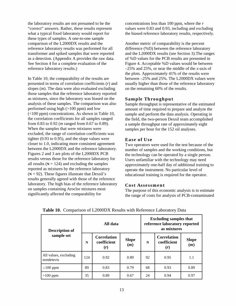
In Table 10, the comparability of the results are presented in terms of correlation coefficients (r) and slopes (m). The data were also evaluated excluding those samples that the reference laboratory reported as mixtures, since the laboratory was biased on the analysis of these samples. The comparison was also performed using high (>100 ppm) and low (<100 ppm) concentrations. As shown in Table 10, the correlation coefficients for all samples ranged from 0.83 to 0.92 (m ranged from 0.67 to 0.89). When the samples that were mixtures were excluded, the range of correlation coefficients was tighter (0.93 to 0.95), and the slope values were closer to 1.0, indicating more consistent agreement between the L2000DX and the reference laboratory. Figures 2 and 3 are plots of the L2000DX PCB results versus those for the reference laboratory for all results (N = 124) and excluding the samples reported as mixtures by the reference laboratory (N = 92). These figures illustrate that Dexsil’s results generally agreed with those of the reference laboratory. The high bias of the reference laboratory on samples containing Aroclor mixtures most significantly affected the comparability for

concentrations less than 100 ppm, where the r values were 0.83 and 0.93, including and excluding the biased reference laboratory results, respectively.

Another metric of comparability is the percent difference (%D) between the reference laboratory and the L2000DX results (see Section 3).The ranges of %D values for the PCB results are presented in Figure 4. Acceptable %D values would be between –25% and 25%, or near the middle of the x-axis of the plots. Approximately 41% of the results were between –25% and 25%. The L2000DX values were usually higher than those of the reference laboratory on the remaining 60% of the results.

Sample Throughput Sample throughput is representative of the estimated amount of time required to prepare and analyze the sample and perform the data analysis. Operating in the field, the two-person Dexsil team accomplished a sample throughput rate of approximately eight samples per hour for the 152 oil analyses.

Ease of Use Two operators were used for the test because of the number of samples and the working conditions, but the technology can be operated by a single person. Users unfamiliar with the technology may need approximately one-half day of additional training to operate the instrument. No particular level of educational training is required for the operator.

Cost Assessment The purpose of this economic analysis is to estimate the range of costs for analysis of PCB-contaminated

Table 10. Comparison of L2000DX Results with Reference Laboratory Data

Description of

All data Excluding samples that

reference laboratory reported as mixtures

sample set

N

Correlation coefficient

(r)

Slope (m)

N

Correlation coefficient

(r)

Slope (m)

All values, excluding nondetects

124 0.92 0.89 92 0.95 1.1

�100 ppm 89 0.83 0.79 68 0.93 0.89

>100 ppm 35 0.89 0.67 24 0.94 0.97

13

L20

00D

X t

otal

PC

B c

once

ntra

tion

(pp

m)

350

300

250

200

150

100

50

0

r = 0.92 m = 0.89

intercept = 22.8 ppm

0 50 100 150 200 250 300 350

Reference laboratory total PCB concentration (ppm)

Figure 2. L2000DX PCB results versus reference laboratory results for all samples.

300

L20

00D

X t

otal

PC

B c

once

ntra

tion

(pp

m)

250

200

150

100

50

0

r = 0.95 m = 1.1

intercept = 11.5 ppm

0 50 100 150 200 250

Reference laboratory total PCB concentration (ppm)

Figure 3. L2000DX PCB results versus reference laboratory results, excluding samples containing mixtures of Aroclors.

14

0

5

10

15

20

25

30

35

-100

to -

75

-74

to -

51

-50

to -

26

-25

to 0

1 to

25

26 to

50

51 to

75

76 to

100

> 1

00

Range of pe rce n t di ffe re nce value s

Num

ber

of s

ampl

es

Figure 4. Range of percent difference (%D) values for PCB results.

oil samples using the L2000DX and a conventional analytical reference laboratory method. The analysis was based on the results and experience gained from this verification test, costs provided by Dexsil, and representative costs provided by the reference analytical laboratory to analyze the samples. To account for the variability in cost data and assumptions, the economic analysis is presented as a list of cost elements and a range of costs for sample analysis by the L2000DX instrument and by the reference laboratory.

Several factors affected the cost of analysis. Where possible, these factors were addressed so that decision makers can complete a site-specific economic analysis to suit their needs. The following categories are considered in the estimate:

• sample shipment costs, • labor costs, and • equipment costs.

Each of these cost factors is defined and discussed and serves as the basis for the estimated cost ranges presented in Table 11. This analysis assumed that the individuals performing the analyses were fully trained to operate the technology. Costs for sample acquisition and pre-analytical sample preparation,

tasks common to both methods, were not included in this assessment.

L2000DX Costs The costs associated with using the L2000DX instrument included labor and equipment costs. No sample shipment charges were associated with the cost of operating the instrument because the samples were analyzed on site.

Labor Labor costs included mobilization and demobili­zation, travel, per diem expenses, and on-site labor.

• Mobilization and demobilization. This cost element included the time for one person to prepare for and travel to each site. This estimate ranged from zero (if the analyst is on site) to 5 h, at a rate of $50/h.

• Travel. This element was the cost for the analyst(s) to travel to the site. If the analyst is located at the site, the cost of commuting to the site would be zero. The estimated cost for an analyst to travel to the site for this verification test ($1000) included the cost of airline travel and rental car fees.

15

Table 11. Estimated analytical costs for PCB-contaminated samples

Analysis method: L2000DX Analyst/manufacturer: Dexsil Corporation Sample throughput: 8 samples/h

Analysis method:Analyst/manufacturer: Typical turnaround:

EPA 600/4-81-045 Reference laboratory 14–30 working days

Cost category Cost ($) Cost category Cost ($)

Sample shipment 0

Labor Mobilization/demobilization Travel Per diem expenses Rate

0-250 0–1,000 per analyst 0–150/day per analyst 30–75/h per analyst

Equipment Mobilization/demobilization Instrument purchase price Instrument lease price Reagents/supplies

0–150 3500 500 per month 5 per sample

Sample shipment Labor Overnight shipping

Labor Mobilization/demobilization Travel Per diem expenses Rate

Equipment

100–200 50–150

Included a

Included Included 10–26 per sample

Included

a “Included” indicates that the cost is included in the labor rate.

• Per diem expenses. This cost element included food, lodging, and incidental expenses. The estimate ranged from zero (for a local site) to $150/day for each analyst.

• Rate. The cost of the on-site labor was estimated at a rate of $30–75/h, depending on the required expertise level of the analyst. This cost element included the labor involved during the entire analytical process, comprising sample preparation, sample management, analysis, and reporting.

Equipment Equipment costs included mobilization and demobilization, rental fees or purchase of equipment, and the reagents and other consumable supplies necessary to complete the analysis.

• Mobilization and demobilization. This included the cost of shipping the equipment to the test site. If the site is local, the cost would be zero. For this verification test, the cost of shipping equipment and supplies was estimated at $150.

• Instrument purchase or lease. The instrument can be purchased for $3500. This price includes enough reagents for 40 tests. The instrument can also be leased for $500 per month. Leasing the instrument requires a prepaid, refundable $2000 deposit.

• Reagents and supplies. Reagents and supplies for the transformer oil analysis are approximately $5 per sample.

Reference Laboratory Costs Sample Shipment The costs of shipping samples to the reference laboratory included overnight shipping charges as well as labor charges associated with the various organizations involved in the shipping process.

• Labor. This cost element included all of the tasks associated with shipping the samples to the reference laboratory. Tasks included packing the shipping coolers, completing the chain-of­custody documentation, and completing the shipping forms. The estimate to complete this task ranged from 2 to 4 h, at $50 per hour.

• Overnight shipping. The overnight express shipping service cost was estimated to be $50 for one 50-lb cooler of samples.

Labor, Equipment, and Waste Disposal The labor bids from commercial analytical reference laboratories that offered to perform the reference analysis for this verification test ranged from $10 to $26 per sample. The bid was dependent on many factors, including the perceived difficulty of the sample matrix, the current workload of the

16

laboratory, data packaging, and the competitiveness of the market. This rate was a fully loaded analytical cost that included equipment, labor, waste disposal, and report preparation.

Cost Assessment Summary An overall cost estimate for use of the L2000DX instrument versus use of the reference laboratory was not made because of the extent of variation in the different cost factors, as outlined in Table 11. The overall costs for the application of any technology would be based on the number of samples requiring analysis, the sample type, and the site location and characteristics. Decision-making factors, such as turnaround time for results, must also be weighed against the cost estimate to determine the value of the field technology’s providing immediate answers versus the reference laboratory’s provision of reporting data within 30 days of receipt of samples.

Miscellaneous Factors The following are general observations regarding the field operation and performance of the L2000DX instrument:

• The L2000DX required no electrical power and worked continuously through a 10-h workday without the need for recharging the battery.

• The Dexsil team was ready for its first set of samples within 2 h of arriving on site.

• The Dexsil team used information on which Aroclors were in the samples to determine the final sample result (based on the instrumental response for each Aroclor). If the Aroclor had been unknown, the calibration curve for Aroclor 1242 would have been used or the result would have been reported as total chloride concentration.

• Tests with the L2000DX generated the following waste: 57 L of TSCA-regulated solids and 2 L of nonregulated liquid/aqueous waste. Careful segregation of the waste could have reduced the volume of TSCA-regulated waste to 4 L.

Summary of Performance A summary of performance is presented in Table 12. Precision, defined as the mean RSD, was 11% for the oil analyses. Accuracy, defined as the mean percent recovery relative to the spiked concentration, was 112%. Of the 20 blank oils, Dexsil reported PCBs in 5 sample (25% false positives). In addition, false positive and false negative results were determined by comparing the L2000DX results with the reference laboratory results for the environmental and spiked samples. One of the results was reported as a false positive (13% fp), but none were false negatives. A one-to­one matching of the L2000DX and reference laboratory results indicates that the results were comparable, with an overall correlation coefficient of 0.92 and a slope value of 0.89. The reference laboratory results were biased high for samples which were mixtures of Aroclors. If those samples are removed from the comparison, the correlation coefficient and slope values improve to 0.95 and 1.1, respectively.

The verification test found that the L2000DX instrument was relatively simple for a trained analyst to operate in the field, requiring less than an hour for initial setup. The sample throughput of the L2000DX was eight samples per hour. Two operators analyzed samples during the verification test, but the technology can be run by a single trained operator. The overall performance of the L2000DX for the analysis of PCBs in transformer oil was characterized as unbiased and precise.

17

Table 12. Performance Summary for the L2000DX

Feature/parameter Performance summary

Precision Mean RSD: 11%

Accuracy Mean recovery: 112%

False positive results on blank samples

25%

False positive results relative to reference laboratory results

13%

False negative results relative to reference laboratory results

None

Comparison with reference laboratory results (all data, excluding suspect values) All values:

Excluding mixtures:

r 0.92 0.95

m 0.89 1.1

Median Absolute% D

31% 31%

Completeness 100% of 152 oil samples

Weight 6 lb

Sample throughput (2 operators) 8 samples/h

Power requirements battery operated (8 V gel cell)

Training requirements One-half day instrument-specific training

Cost Purchase: $3,500 Lease: $500 per month (plus $2,000 refundable deposit) Reagents/Supplies: $5 per oil sample

Waste generated 57 L of TSCA-regulated solids (which could have been r 4 L by segregation of the waste) 2 L of nonregulated liquid/aqueous waste (Total number of samples analyzed: 152)

educed to

Overall evaluation Precise Unbiased

18

Section 6 — References

ASTM (American Society for Testing and Materials). 1997a. Standard Practice for Generation of Environmental Data Related to Waste Management Activities: Quality Assurance and Quality Control Planning and Implementation. D5283-92.

ASTM (American Society for Testing and Materials). 1997b. Standard Practice for Generation of Environmental Data Related to Waste Management Activities: Development of Data Quality Objectives. D5792-95.

Berger, W., H. McCarty, and R-K. Smith. 1996. Environmental Laboratory Data Evaluation. Genium Publishing Corp., Schenectady, N.Y.

Draper, N. R., and H. Smith. 1981. Applied Regression Analysis. 2nd ed. John Wiley & Sons, New York.

EPA (U.S. Environmental Protection Agency). 1982. Test Method: The Determination of Polychlorinated Biphenyls in Transformer Fluid and Waste Oils. EPA/600/4-81-045. U.S. Environmental Protection Agency, Washington, D.C., September.

EPA (U.S. Environmental Protection Agency). 1994. “Method 8081: Organochlorine Pesticides and PCBs as Aroclors by Gas Chromatography: Capillary Column Technique.” In Test Methods for Evaluating Solid Waste: Physical/Chemical Methods (SW-846). 3d ed., Final Update II. Office of Solid Waste and Emergency Response, Washington, D.C., September.

EPA (U.S. Environmental Protection Agency). 1996. Guidance for Data Quality Assessment. EPA QA/G-9; EPA/600/R-96/084. EPA, Washington, D.C., July.

EPA (U.S. Environmental Protection Agency). 1998. Environmental Technology Verification Report: Electrochemical Technique/Ion Specific Electrode, Dexsil Corporation, L2000 PCB/Chloride Analyzer. EPA/600/R-98/109. U.S. Environmental Protection Agency, Washington, D.C., August.

Erickson, M. D. 1997. Analytical Chemistry of PCBs. 2nd ed. CRC Press/Lewis Publishers, Boca Raton, Fla.

ORNL (Oak Ridge National Laboratory). 2000. Technology Verification Test Plan: Evaluation of Polychlorinated Biphenyl (PCB) Field Analytical Techniques. Chemical and Analytical Sciences Division, Oak Ridge National Laboratory, Oak Ridge, Tenn., August.

19

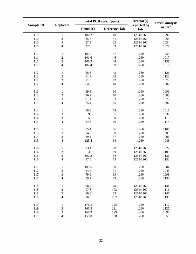
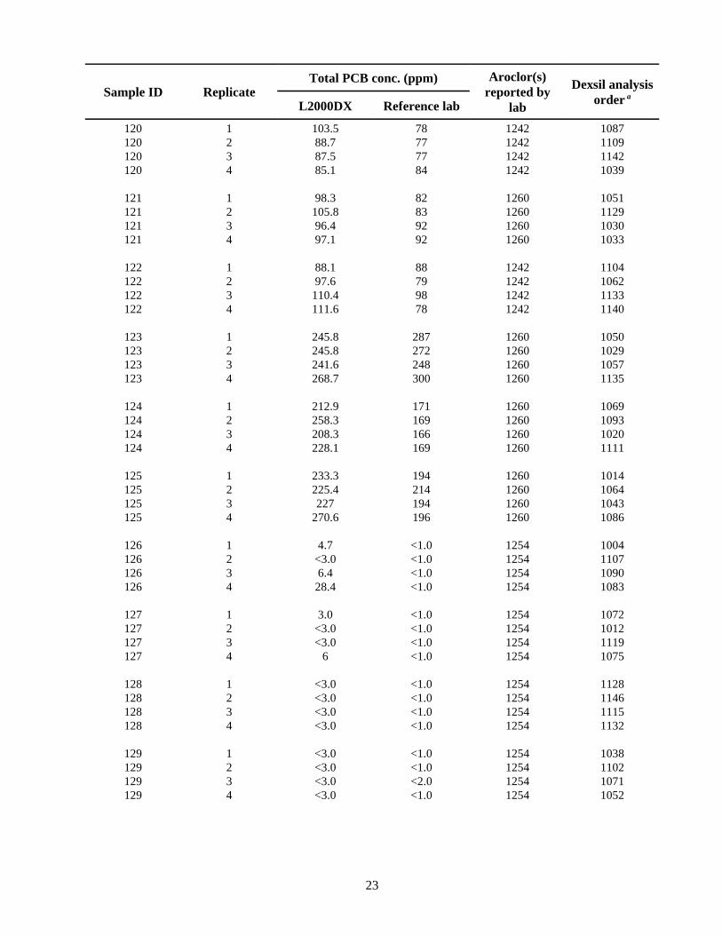
Appendix A

Dexsil’s L2000DX Results Compared withReference Laboratory Results

Sample ID Replicate Total PCB conc. (ppm)

L2000DX Reference lab

Aroclor(s) reported by

lab

Dexsil analysis order a

101 101 101 101

1 2 3 4

<3.0 <3.0 <3.0 <3.0

<1.0 <1.0 <1.0 <1.0

1254 1254 1254 1254

1108 1010 1067 1027

102 102 102 102

1 2 3 4

<3.0 3

<3.0 <3.0

<1.0 <1.0 <1.0 <1.0

1254 1254 1254 1254

1123 1001 1005 1054

103 103 103 103

1 2 3 4

10.4 10 9.3 9.4

3 2 1 2

1260 1260 1260 1260

1035 1137 1053 1056

104 104 104 104

1 2 3 4

9.1 11.1 12 7.5

4 3 2 2

1260 1260 1260 1260

1023 1149 1074 1118

105 105 105 105

1 2 3 4

23.9 25.1 19.6 15.2

8 9

12 10

1260 1260 1260 1260

1078 1085 1141 1046

106 106 106 106

1 2 3 4

38.8 41.7 39.3 38.8

15 11 14 16

1260 1260 1260 1260

1068 1036 1013 1063

107 107 107 107

1 2 3 4

54.2 53.7 55.4 61.9

21 21 23 23

1260 1260 1260 1260

1031 1016 1044 1145

108 108 108 108

1 2 3 4

39.4 42.1 40.4 41

23 25 20 26

1260 1260 1260 1260

1058 1026 1143 1019

109 109 109 109

1 2 3 4

70.8 74.2 73.2 79.4

26 27 24 32

1242/1254 1242/1254 1242/1254 1242/1254

1049 1037 1042 1127

21

Sample ID Replicate Total PCB conc. (ppm)

L2000DX Reference lab

Aroclor(s) reported by

lab

Dexsil analysis order a

110 110 110 110

1 2 3 4

100.2 85.8 87.9 101

40 41 32 33

1254/1260 1254/1260 1254/1260 1254/1260

1092 1065 1034 1077

111 111 111 111

1 2 3 4

103.1 101.6 108.3 102.4

37 45 44 39

1260 1260 1260 1260

1055 1017 1151 1015

112 112 112 112

1 2 3 4

58.3 61.4 71.5 64.8

43 35 42 40

1260 1260 1260 1260

1121 1122 1079 1002

113 113 113 113

1 2 3 4

89.8 96.2 81.1 75.4

80 70 93 65

1260 1260 1260 1260

1091 1080 1073 1097

114 114 114 114

1 2 3 4

60.6 59 65

64.6

64 65 58 56

1260 1260 1260 1260

1018 1032 1113 1114

115 115 115 115

1 2 3 4

85.4 84.8 89.4

125.4

66 90 67 64

1260 1260 1260 1260

1105 1009 1096 1088

116 116 116 116

1 2 3 4

93.1 84

102.2 97.6

58 59 64 75

1254/1260 1254/1260 1254/1260 1254/1260

1022 1103 1136 1152

117 117 117 117

1 2 3 4

103.5 84.8 79.6 89.4

68 81 69 69

1260 1260 1260 1260

1084 1048 1098 1130

118 118 118 118

1 2 3 4

98.2 97.8 90.8 86.8

79 102 83

102

1254/1260 1254/1260 1254/1260 1254/1260

1131 1116 1147 1138

119 119 119 119

1 2 3 4

178.5 166.2 168.9 159.8

125 131 129 130

1260 1260 1260 1260

1117 1125 1095 1059

22

Sample ID Replicate Total PCB conc. (ppm)

L2000DX Reference lab

Aroclor(s) reported by

lab

Dexsil analysis order a

120 120 120 120

1 2 3 4

103.5 88.7 87.5 85.1

78 77 77 84

1242 1242 1242 1242

1087 1109 1142 1039

121 121 121 121

1 2 3 4

98.3 105.8 96.4 97.1

82 83 92 92

1260 1260 1260 1260

1051 1129 1030 1033

122 122 122 122

1 2 3 4

88.1 97.6

110.4 111.6

88 79 98 78

1242 1242 1242 1242

1104 1062 1133 1140

123 123 123 123

1 2 3 4

245.8 245.8 241.6 268.7

287 272 248 300

1260 1260 1260 1260

1050 1029 1057 1135

124 124 124 124

1 2 3 4

212.9 258.3 208.3 228.1

171 169 166 169

1260 1260 1260 1260

1069 1093 1020 1111

125 125 125 125

1 2 3 4

233.3 225.4 227

270.6

194 214 194 196

1260 1260 1260 1260

1014 1064 1043 1086

126 126 126 126

1 2 3 4

4.7 <3.0 6.4

28.4

<1.0 <1.0 <1.0 <1.0

1254 1254 1254 1254

1004 1107 1090 1083

127 127 127 127

1 2 3 4

3.0 <3.0 <3.0

6

<1.0 <1.0 <1.0 <1.0

1254 1254 1254 1254

1072 1012 1119 1075

128 128 128 128

1 2 3 4

<3.0 <3.0 <3.0 <3.0

<1.0 <1.0 <1.0 <1.0

1254 1254 1254 1254

1128 1146 1115 1132

129 129 129 129

1 2 3 4

<3.0 <3.0 <3.0 <3.0

<1.0 <1.0 <2.0 <1.0

1254 1254 1254 1254

1038 1102 1071 1052

23

Sample ID Replicate Total PCB conc. (ppm)

L2000DX Reference lab

Aroclor(s) reported by

lab

Dexsil analysis order a

130 130 130 130

1 2 3 4

<3.0 <3.0 <3.0 3.4

<1.0 <1.0 <1.0 <1.0

1254 1254 1254 1254

1008 1124 1025 1076

131 131 131 131

1 2 3 4

4 5.1 7

15.7

6 4 5 6

1254 1254 1254 1254

1110 1099 1139 1081

132 132 132 132

1 2 3 4

24.2 22.3 24.2 26.4

21 21 20 25

1260 1260 1260 1260

1150 1070 1007 1089

133 133 133 133

1 2 3 4

33.1 39

44.3 39.7

51 54 50 54

1254/1260 1254/1260 1254/1260 1254/1260

1106 1126 1066 1120

134 134 134 134

1 2 3 4

45.8 51.1 54.2 49.1

57 74 61 67

1254/1260 1254/1260 1254/1260 1254/1260

1061 1040 1144 1047

135 135 135 135

1 2 3 4

59.6 63.8 56.7 52

78 76 79 78

1254/1260 1254/1260 1254/1260 1254/1260

1148 1041 1024 1060

136 136 136 136

1 2 3 4

64.6 84.4 98.3 85.2

83 64 73 73

1260 1260 1260 1260

1006 1134 1101 1003

137 137 137 137

1 2 3 4

107.4 98.8 94.1

130.6

86 86

108 109

1254 1254 1254 1254

1112 1028 1021 1100

138 138 138 138

1 2 3 4

175.4 271.9 233.9 186.2

260 261 255 249

1254/1260 1254/1260 1254/1260 1254/1260

1045 1094 1082 1011

a These are the sample numbers from which the analysis order can be discerned. For example, 1001 was the first sample analyzed, then 1002, etc.

24

Appendix B

Data Quality Objective (DQO) Example

Disclaimer The following hypothetical example serves to demonstrate how the information provided in this report may be used in the data quality objectives (DQO) process. This example serves to illustrate the application of quantitative DQOs to a decision process but cannot attempt to provide a thorough education in this topic. Please refer to other educational or technical resources for further details (ASTM 1997a, b; EPA 1996). In addition, since the focus of this report is on the analytical technology, this example makes the simplifying assumption that the sample will be homogeneous. In the real world, however, this assumption is seldom valid, and matrix heterogeneity constitutes a source of considerable uncertainty that must be adequately evaluated if the overall certainty of a site decision is to be quantified.

Background and Problem Statement An industrial company discovered a warehouse of transformers which were filled with PCB-containing oils. The contaminated oil was transferred into waste drums. Preliminary characterization determined that the PCB concentration in a single drum was homogenous but that PCB concentrations varied greatly from drum to drum. The company’s DQO team was considering the use of Dexsil’s L2000DX to measure the PCB concentration in each drum. The DQO team decided that drums would be disposed of by incineration if the PCB concentration was �50 ppm (“hot”). The concentration of 50 ppm is the Toxic Substances Control Act (TSCA) regulatory threshold (RT) for this environmental problem. Those drums with PCB concentrations <50 ppm would be put into a landfill because incineration of oil is very expensive. With regulator agreement, the DQO team determined that a decision rule for disposal would be based on the average concentration of PCBs in each drum.

General Decision Rule

If average PCB Concentration < 50 ppm, then send the oil drum to the landfill.

If average PCB Concentration � 50 ppm, then send the oil drum to the incinerator.

DQO Goals The DQO team’s primary goal was to calculate how many samples would need to be analyzed by the L2000DX Analyzer in order to confidently make a decision about disposing of the oil, given the uncertainties of the technology’s results. Because the team decided that inadvertently sending oil to the landfill that exceeded the 50 ppm concentration of PCBs was the worst possible mistake, the number of samples measured was primarily related to this false rejection decision error rate. A secondary decision error would be to incinerate unnecessarily the drum that contained PCB concentrations <50 ppm, which would be a false acceptance decision error. Both the false rejection decision error and the false acceptance decision error were taken into account to determine the final sampling plan.

The team required that the error rate for sending a “hot” drum to the landfill (i.e., the false rejection error rate for the decision) could not be more than 5%. Therefore, a sufficient number of samples had to be taken from each drum to ensure that the false rejection decision error rate (FR) would be 0.05 (or less) that the true drum concentration is 50 ppm. This scenario represents a 5% chance of sending a drum containing PCB concentrations �50 ppm to the landfill.

25

The DQO team did not want to send an excessive number of drums to the incinerator if the average PCB concentration was <50 ppm because of the expense. In this situation, a false acceptance decision is made when it is concluded that a drum is “hot,” when in actuality, the drum contains oil with <50 ppm PCBs. Therefore, the team recommended that the false acceptance decision error rate (FA) be 0.10 if the true drum concentration was 40 ppm. That is, there would be a 10% probability of sending a drum to the incinerator (denoted as Pr[Take Drum to Incinerator]) if the true PCB concentration for a drum was 40 ppm.

Permissible FR and FA Error Rates and Critical Decision Points

FR: Pr[Take Drum to Landfill] �0.05 when true PCB concentration = 50 ppm

FA: Pr[Take Drum to Incinerator] �0.10 when true PCB concentration = 40 ppm

Use of Technology Performance Information to Implement the Decision Rule Technology performance information is used to evaluate whether a particular analytical technology can produce data of sufficient quality to support the site decision. Because the DQO team was considering the use of the L2000DX, the performance of this technology (as reported in this ETV report) was used to assess its applicability to this project. Two questions arise:

1. How many samples are needed from a single drum to permit a valid estimation of the true average concentration of PCBs in the drum to the specified certainty? Recall that the simplifying assumption was made that the PCB distribution throughout the oil within a single drum is homogeneous and thus, matrix heterogeneity will not contribute to overall variability. The only variability to be considered in this example, then, is the variability in the L2000DX’s analytical method, which is determined by precision studies.

2. What is the appropriate action level (AL) for using the Dexsil L2000DX to make decisions in the field? After the required number of samples have been collected from a drum and analyzed, the results are averaged together to get an estimate of the “true” PCB concentration of the drum. When using the L2000DX, what is the value (here called “the action level for the decision rule”) to which that average is compared, to decide if the drum is “hot” or not? This method-specific or site-specific action level is derived from evaluations of the method’s accuracy using an appropriate quality control regimen.

L2000DX Analyzer Accuracy The ETV verification results indicated that the PCB concentrations determined by the L2000DX were unbiased when compared with concentration values for performance evaluation samples. Also, the concentration measurements with the L2000DX had a strong linear correlation (r = 0.92) with the concentration values measured by the reference laboratory using EPA Method 600/4-81-045 (EPA 1982). Figure B-1 shows a linear relationship between L2000DX’s PCB concentrations and the certified PCB values for the performance evaluation samples, which were in the concentration range of 0 to 60 ppm. The equation for the PCB prediction line is:

L2000DX result = –2.51 + 0.93 × (Certified PE Value) (Eq. B-1)

There is no significant difference at the 5% significance level between the intercept value and zero, and the slope value and 1, in Eq. B-1. The L2000DX measurements were therefore unbiased for this concentration range.

26

0 10 20 30 40 50 60

60

50

40

30

20

10

0

Certified PCB Concentration (ppm)

Figure B-1. A linear model for predicting L2000DX PCB

Avg

L20

00DX

PCB

Con

cent

ratio

n (p

pm)

concentrations from certified PCB concentrations with 95% confidence intervals (dashed lines).

Determining the Number of Samples With the critical decision points selected, the team could then determine the number of samples needed from each drum to calculate the drum’s “true” average PCB concentration. For a homogeneous matrix, the number of samples required depends on the precision of the analytical method.

As can be seen in Figure B-2, the standard deviations do not increase with increasing certified concentrations for the range of interest from 5 to 60 ppm. Therefore, the precision of the L2000DX can be represented by a pulled standard deviation of 4.2 ppm within the concentration range of 5 to 60 ppm (see Figure B-2). The pulled standard deviation is calculated by first calculating the average variance and then taking the square root. This estimate of analytical variability (precision) is used to calculate the number of oil samples required to be analyzed from each drum to achieve the DQOs as determined above under

“DQO Goals.” A formula is provided in EPA’s Guidance for Data Quality Assessment (EPA 1996, pp. 3.2–3, Box 3.2-1) that can be adapted to this example for calculating the number of samples required to meet the FR and FA requirements:

(Eq. B-2)

6

where

0 10 20 30 40 50 60

N = number of samples from a drum to be measured

S2 = variance for the measurement [e.g., S2 = (4.2) 2 ]

RT = regulatory threshold (e.g., RT = 50 ppm)

CFA = concentration at which FA is specified (e.g., CFA = 40 ppm)

FR = false rejection decision error rate (e.g., FR = 0.05)

FA = false acceptance decision error rate(e.g., FA = 0.10) L2

000D

X St

anda

rd D

evia

tion

(ppm

) 5

4

3

2

1

Certified PCB Concentration (ppm)

Figure B-2. Regression of L2000DX standard deviations

versus certified PCB concentrations.

27

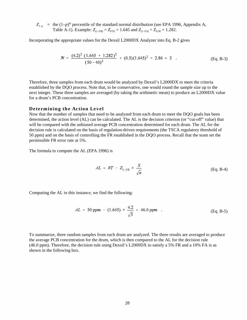
Z1–p = the (1–p)th percentile of the standard normal distribution (see EPA 1996, Appendix A, Table A-1). Example: Z(1–FR) = Z0.95 = 1.645 and Z(1–FA) = Z0.90 = 1.282.

Incorporating the appropriate values for the Dexsil L2000DX Analyzer into Eq. B-2 gives

Therefore, three samples from each drum would be analyzed by Dexsil’s L2000DX to meet the criteria established by the DQO process. Note that, to be conservative, one would round the sample size up to the next integer. These three samples are averaged (by taking the arithmetic mean) to produce an L2000DX value for a drum’s PCB concentration.

Determining the Action Level Now that the number of samples that need to be analyzed from each drum to meet the DQO goals has been determined, the action level (AL) can be calculated. The AL is the decision criterion (or “cut-off” value) that will be compared with the unbiased average PCB concentration determined for each drum. The AL for the decision rule is calculated on the basis of regulation-driven requirements (the TSCA regulatory threshold of 50 ppm) and on the basis of controlling the FR established in the DQO process. Recall that the team set the permissible FR error rate at 5%.

The formula to compute the AL (EPA 1996) is

(Eq. B-3)

(Eq. B-4)

Computing the AL in this instance, we find the following:

(Eq. B-5)

To summarize, three random samples from each drum are analyzed. The three results are averaged to produce the average PCB concentration for the drum, which is then compared to the AL for the decision rule (46.0 ppm). Therefore, the decision rule using Dexsil’s L2000DX to satisfy a 5% FR and a 10% FA is as shown in the following box.

28

Decision Rule for FR = 5% and FA = 10%

If the average PCB concentration of three random oil samples from a drum is <46.0 ppm, then send the drum to the landfill.

If the average PCB concentration of three random oil samples from a drum is �46.0 ppm, then send the drum to the incinerator.

The decision performance curve calculates the 1.0

probability of sending a drum to the incinerator 0.9

for different values of true PCB oil concentration

35 40 45 50 55

False Positive = 5%

in a drum (for more information, see EPA 1996, 0.8

pp. 34–36). Figure B-3 shows that the decision performance curve has the value of Pr[ Take Drum to Incinerator] = 0.95 for True = 50 ppm. This indicates that the decision rule meets the DQO team’s FR of 5%. The Pr[ Take Drum to Incinerator] = 0.007 for True = 40 ppm, which is better than the FA of 10% that the DQO team had originally specified. This improved performance is due to rounding up the number of samples to the next integer in the calculation of number of samples required. Pr

ob[ T

ake

Drum

to In

cine

rato

r ]

0.7

0.6

0.5

0.4

0.3

0.2

0.1

0.0

Alternative FR Parameter Because of random sampling and analysis error, True PCB Concentration (ppm) there is always some chance that analytical Figure B-3. Decision performance curve for PCB drum

results will not accurately reflect the true nature example. of a decision unit (such as a drum, in this example). Often, 95% certainty (a 5% FR) is customary and sufficient to meet stakeholder comfort. But suppose that the DQO team wanted to be even more cautious about limiting the possibility that a drum might be sent to a landfill when its true value is 50 ppm. If the team wanted to be 99% certain that a drum was correctly sent to a landfill, the following describes how changing the FR requirement from 5% to 1% would affect the decision rule.

Using FR = 0.01, the sample size is calculated to be 6 and the AL is calculated as 46.0 ppm. (That this calculation is the same AL as before is coincidental.) The decision performance curve has the value of Pr[Take Drum to Incinerator] = 0.99 for True = 50 ppm. This indicates that the decision rule meets the DQO team’s FR of 1%. The Pr[ Take Drum to Incinerator] = 0.0002 for True = 40 ppm is better than the FA of 10% that the DQO team had specified. This improved performance is due to rounding up the number of samples to the next integer in the calculation of number of samples required. The decision rule for the lower FR would be as shown in the following box.

29

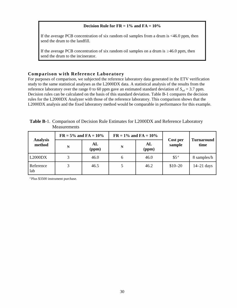
Decision Rule for FR = 1% and FA = 10%

If the average PCB concentration of six random oil samples from a drum is <46.0 ppm, then send the drum to the landfill.

If the average PCB concentration of six random oil samples on a drum is �46.0 ppm, then send the drum to the incinerator.

Comparison with Reference Laboratory For purposes of comparison, we subjected the reference laboratory data generated in the ETV verification study to the same statistical analyses as the L2000DX data. A statistical analysis of the results from the reference laboratory over the range 0 to 60 ppm gave an estimated standard deviation of Sref = 3.7 ppm. Decision rules can be calculated on the basis of this standard deviation. Table B-1 compares the decision rules for the L2000DX Analyzer with those of the reference laboratory. This comparison shows that the L2000DX analysis and the fixed laboratory method would be comparable in performance for this example.

Table B-1. Comparison of Decision Rule Estimates for L2000DX and Reference LaboratoryMeasurements

Analysis method

FR = 5% and FA = 10% FR = 1% and FA = 10% Cost per sample

Turnaround timeN

AL (ppm)

N AL

(ppm)

L2000DX 3 46.0 6 46.0 $5 a 8 samples/h

Reference lab

3 46.5 5 46.2 $10–20 14–21 days

a Plus $3500 instrument purchase.

30