pcc vivace: online-learning congestion control - usenix.org · scheme. vivace adopts the high-level...

This paper is included in the Proceedings of the 15th USENIX Symposium on Networked

Systems Design and Implementation (NSDI ’18).April 9–11, 2018 • Renton, WA, USA

ISBN 978-1-931971-43-0

Open access to the Proceedings of the 15th USENIX Symposium on Networked

Systems Design and Implementation is sponsored by USENIX.

PCC Vivace: Online-Learning Congestion ControlMo Dong and Tong Meng, UIUC; Doron Zarchy, The Hebrew University of Jerusalem;

Engin Arslan, UIUC; Yossi Gilad, MIT; Brighten Godfrey, UIUC; Michael Schapira, The Hebrew University of Jerusalem

https://www.usenix.org/conference/nsdi18/presentation/dong

PCC Vivace: Online-Learning Congestion Control

Mo Dong*, Tong Meng*, Doron Zarchy†, Engin Arslan‡, Yossi Gilad§,P. Brighten Godfrey* and Michael Schapira†

*UIUC, †Hebrew University of Jerusalem, ‡University of Nevada, Reno, §MIT

Abstract

TCP’s congestion control architecture suffers from no-toriously bad performance. Consequently, recent yearshave witnessed a surge of interest in both academia andindustry in novel approaches to congestion control. Weshow, however, that past approaches fall short of at-taining ideal performance. We leverage ideas from therich literature on online (convex) optimization in machinelearning to design Vivace, a novel rate-control protocol,designed within the recently proposed PCC framework.Our theoretical and experimental analyses establish thatVivace significantly outperforms traditional TCP vari-ants, the previous realization of the PCC framework, andBBR in terms of performance (throughput, latency, loss),convergence speed, alleviating bufferbloat, reactivity tochanging network conditions, and friendliness towardslegacy TCP in a range of scenarios. Vivace requires onlysender-side changes and is thus readily deployable.

1 Introduction

The recent surge of interest in both academia and in-dustry in improving Internet congestion control [8, 11,13, 19, 21, 22, 24, 25, 31, 32, 36] has made it appar-ent that today’s prevalent congestion control algorithms,the TCP family, fall short of important performance re-quirements. Indeed, transport rate control faces numer-ous challenges. First and foremost, a congestion con-trol architecture should be able to efficiently utilize net-work resources under varying and complex network con-ditions. This includes optimizing for throughput, loss,and latency, and doing so in a plethora of environments— potentially with non-congestion loss [8], high-RTTcross-continent links, highly dynamic networks such asWiFi and LTE links, etc. Second, congestion controlshould guarantee quick convergence to stable and fairrates when multiple senders compete over network re-sources. This desideratum is particularly important forapplications like high quality or virtual reality video

streaming. Last, a congestion control scheme should beeasy and safe (e.g., sufficiently friendly to existing pro-tocols) to deploy.

Traditional algorithms [6, 15, 23] fail to satisfy thefirst two requirements; their performance can be as highas 10× away from the optimal under non-congestionpacket loss [11]. Recent proposals, including Remy [31],PCC [11], and BBR [8], investigate new approachesto this challenge. Remy replaces the human designerwith an offline optimization scheme that searches for thebest scheme within a certain design space, for a pre-specified range of network conditions. While they canattain high performance, Remy-generated TCPs are in-herently prone to degraded performance when the actualnetwork conditions deviate from input assumptions [27].

BBR takes a white-box network-modeling approach,translating change patterns in performance measure-ments (e.g., increase in delivery rate) to presumed un-derlying network conditions (e.g., bottleneck through-put and latency). PCC takes a black box approach: aPCC sender observes performance metrics resulting fromsending at a specific rate, converts these metrics into anumerical utility value, and adapts the sending rate in thedirection that empirically is associated with higher util-ity. Our experiments indicate that while improving sub-stantially over traditional schemes, both the specific real-ization of PCC in [11], termed “PCC Allegro” (or sim-ply Allegro) henceforth, and BBR’s implementation [8],fail to achieve optimal low latency and exhibit far-from-ideal tradeoffs between convergence speed and stabil-ity. Specifically, BBR exhibits high rate variance andhigh packet loss rate upon convergence, whereas PCCAllegro’s convergence time is overly long. In addition,when BBR’s model of the network does not reflect thecomplexities of reality, performance can suffer severely.Lastly, they are both highly aggressive towards TCP, al-though BBR is designed with TCP-friendliness in mind.

To address the above limitations, we draw inspirationfrom literature on online (convex) optimization [12, 16,37] to design PCC Vivace, a novel congestion control

USENIX Association 15th USENIX Symposium on Networked Systems Design and Implementation 343

scheme. Vivace adopts the high-level architecture ofPCC – a utility function framework and a learning rate-control algorithm – but realizes both components dif-ferently. First, Vivace relies on a new, learning-theory-informed framework for utility derivation that incorpo-rates crucial considerations such as latency minimizationand TCP friendliness. Second, Vivace employs prov-ably (asymptotically) optimal online optimization basedon gradient ascent to achieve high utilization of networkcapacity, swift reaction to changes, and fast and stableconvergence. In particular, our contributions are:

(1) A principled framework for transport utility withmultiple novel consequences. We prove that for aproper choice of utility functions that incorporate notonly throughput and loss (as in Allegro), but also la-tency, a stable global rate configuration (Nash equilib-rium) always exists; show a tradeoff between randomloss tolerance and packet loss at convergence with com-peting senders; and allow controllable capacity alloca-tion among competing senders with heterogeneous utili-ties (suggesting a future opportunity for centralized net-work control in an SDN or OpenTCP [13] architecture).

(2) A rate control scheme that utilizes gradient-ascentalgorithms from online learning theory to achieve animproved tradeoff between stability and reactivity. Weprove that our rate-control scheme guarantees quick con-vergence to the equilibrium guaranteed by our choiceof utility functions, and employ additional techniques toimprove rate control in the face of noisy measurements,such as linear regression and low-pass filtering.

(3) Extensive experiments with PCC Vivace, PCC Al-legro, BBR, and various TCP variants, in controlled en-vironments, real residential Internet scenarios, and withvideo-streaming applications. Highlights include: im-proved performance in rapidly changing conditions (70%less packet loss and 72.5% higher throughput than PCCAllegro, and around 20% median throughput gain overBBR); convergence about 2× faster than Allegro and sta-bility about 2× better than BBR; 57% less video buffer-ing time than BBR with multiple ongoing streams; andsignificantly improved TCP friendliness.

By no means do we expect that Vivace is the end ofthe story. Optimizing rate quickly and accurately withlimited information in a complex, noisy environment isdifficult, and we highlight a simulated LTE environmentwhere a “white-box” model-based approach engineeredfor this context, namely Sprout [32], outperforms Vi-vace, as a case for future work. However, Vivace repre-sents a substantial overall advance, showing how a stronglearning-theoretic basis yields practical improvements.

2 Rate-Control Through Online LearningWhen approached from an online learning perspective,the challenges outlined in § 1 fall naturally into the cat-

egory of online optimization in machine learning andgame theory [16, 37] (a.k.a. “no-regret learning”). On-line learning provides a useful and powerful abstractionfor decision making under uncertainty. In the onlinelearning setting, a decision maker repeatedly selects be-tween available strategies. Only after selection is the de-cision maker aware of the implications of the selectedstrategy, in terms of a resulting utility value. State-of-the-art online learning algorithms provide provable guaran-tees (namely, the classical “no regret” guarantee [16, 37])even under complete uncertainty about the environment,i.e., without assuming/inferring anything about the rela-tion between choices of strategies and the induced utilityvalues. In addition, results in game theory establish thatonline learning algorithms “play well” together, in thesense that, under the appropriate conditions, global con-vergence to a stable equilibrium is guaranteed when thereare multiple decision makers.

We are thus inspired to apply ideas and machineryfrom online learning to rate control on the Internet, whichcan naturally be cast as an online learning task as follows.A traffic sender repeatedly selects between sending rates.After sending at a certain rate for “sufficiently long”, thesender learns its performance implications by translatingaggregated statistics (e.g., achieved goodput, packet lossrate, average latency) into a numerical utility value, andthen adapts the sending rate in response. Importantly, theapplication of online learning to rate-control is particu-larly challenging since often only very limited feedbackfrom the network is available to the sender, and so accu-rately determining the utility derived from sending at acertain rate is sometimes infeasible.

PCC [11] is a promising step towards online-learning-based congestion control. The gist of its architecture isas follows. Time is divided into consecutive intervals,called Monitor Intervals (MIs), each devoted to “testing”the implications for performance of sending at a certainrate. PCC aggregates selective ACKs for packets sent ina MI into the above-mentioned meaningful performancemetrics, and feeds these metrics into a utility functionthat translates them into a numerical value. PCC’s rate-control module continuously adjusts the sending rate inthe direction that is most beneficial in terms of utility.

However, the specific realization of PCC Allegroin [11] is far from tapping the full potential of onlinelearning. First, Allegro uses a somewhat arbitrary choiceof utility function. While [11] proves this choice inducesdesirable properties in some settings, fair convergenceis not provably guaranteed when utility functions arelatency-aware, reasoning about fundamental tradeoffs inparameter settings is difficult, and there is no theoreti-cal understanding of what happens when Allegro senderswith different utility functions interact with each other.

Second, Allegro inherently ignores the information re-

344 15th USENIX Symposium on Networked Systems Design and Implementation USENIX Association

Figure 1: Utility-based rate-controlflected in the utility when deciding on step size. Sup-pose Allegro’s utility function is as described in Fig-ure 1, where C is the capacity of a single link. Then,consider two possible initial rates for the Allegro-sender:r1 and r2 (r1 < C� r2). When starting at r1, the Alle-gro sender will increase its rate to r1(1+ ε), for a fixedε > 0, whereas the initial rate r2 will be followed by adecrement to r2(1− ε). Intuitively, this rate-adjustmentis not optimal; a small ε will result in slowly lowering therate from r2, leading to long convergence time, whereaschoosing too large an ε will increase the rate from r1by too much, overshooting the optimum. Indeed, anychoice of fixed increase/decrease step size is bound to betoo much in some circumstances and too little in others,resulting in suboptimal reactivity or convergence.

The combination of Allegro’s fairly naive rate controlscheme and its ad hoc choice of utility function preventsit from attaining good performance under rapidly chang-ing network conditions, does not alleviate bufferbloat,results in convergence rate/stability tradeoff that is bet-ter TCP’s yet still suboptimal, leads to high packet lossupon convergence, and is overly aggressive towards TCP.Hence, despite a promising architecture, the operationalinstantiation of PCC in [11] is still far from optimal.

To address the above limitations, Vivace’s design bor-rows ideas from the rich body of literature on online con-vex optimization [12, 16, 37] to replace the realization ofthe two crucial components of PCC’s high-level architec-ture: (1) the utility function framework, and (2) the learn-ing rate-control algorithm. First, Vivace relies on a new,learning-theory-informed framework for utility deriva-tion [12], which guarantees multiple competing Vivacesenders will converge to a unique stable rate configura-tion that is fair and near-optimal. Second, Vivace em-ploys provably optimal gradient-ascent-based no-regretonline optimization [37] to adjust sending rates, takinginto account not only the direction (increase/decrease)that is more beneficial utility-wise, but also the extent towhich increasing/decreasing the rate impacts utility.No-regret learning. The classical objective in onlinelearning theory is regret minimization. We give an infor-mal exposition of the implications of no-regret for con-gestion control here. See [16, 37] for a more completetreatment. A “no-regret” rate-control protocol, such asVivace, guarantees that its choices of rates are asymptot-ically (across time) no worse, utility-wise, than sendingat what would have been (in hindsight) the best fixed rate.

No-regret is a useful guarantee for two reasons.First, no-regret provides a formal performance guaran-

tee for individual senders across all network conditions,even highly dynamic or adversarially chosen (within thescope of the model). We believe Vivace is the first con-gestion control scheme to provide such a guarantee.

Second, no-regret provides a powerful lens for theo-retical analysis, which we will use to reason formallyabout convergence with multiple competing no-regretsenders, even with heterogeneous utility functions acrossthe senders, and also about tradeoffs between resilienceto non-congestion loss and loss upon convergence.

Limitations of no-regret. As no-regret relates perfor-mance to the best fixed strategy, the quality of this guar-antee in a dynamic environment depends on the speed atwhich the protocol minimizes “regret” [16]. If, from anarbitrary starting state, the regret vanishes to a desiredlow value within T time units, then the no-regret guar-antee applies relative to the best fixed strategy within ev-ery T units of time. Empirically (§5.1.4), Vivace adaptsquickly to changes in network conditions.

Of course, a guarantee of near-optimality relative tothe best dynamic strategy would be even better. However,such guarantees often entail assumptions about the en-vironment, e.g., that the network behavior exhibits highregularity. Vivace reflects the design choice of avoidingsuch assumptions. That said, an important direction forfuture research is to quantify to what extent real-worldnetworks are sufficiently predictable (e.g., via machinelearning) to improve rate selection.PCC Allegro vs. PCC Vivace. Compared with PCC Al-legro, PCC Vivace’s utility framework (1) incorporateslatency awareness, mitigating the bufferbloat problemand the resulting packet loss and latency inflation, (2)extends to heterogeneous senders with different utilityfunctions, enabling flexible network-resource allocation,and (3) induces more friendly behavior towards TCP, andthus is better suited for real-world deployment. In addi-tion, Vivace’s rate-control algorithm (1) provides faster,more stable convergence, and (2) reacts more quicklyupon changes to network conditions.

3 Vivace’s Utility FrameworkVivace divides time into consecutive Monitor Intervals(MIs). At the end of each MI, sender i applies the follow-ing utility function to transform the performance statis-tics gathered at that MI to a numerical utility value:

u(

xi,d(RT Ti)

dT,Li

)= xt

i−bxid(RT Ti)

dT− cxi×Li, (1)

where 0< t < 1,b≥ 0,c> 0, xi is sender i’s sending rate,and Li is its observed loss rate. The term d(RT Ti)

dT is the ob-served “RTT gradient” during this MI, i.e., the increase inlatency experienced within this MI. The parameters b,c, tare constants. Intuitively, utility functions of the above


form reward increase in throughput (via xti), and penalize

increase in both latency (bxid(RT Ti)

dT ) and loss (cxi×Li).We next identify the properties of utility functions withinour framework, and refer to [2] for formal analysis.

To see why Vivace’s utility function does not considerthe absolute value of latency, instead using RTT gradi-ent, consider the following example. A single sender ona link with a large buffer sends at a rate of twice the ca-pacity of the link for a single MI; then, in the next MI,it tries a slightly lower but still over-capacity rate. Sucha sender would experience higher absolute latency in thesecond MI than in the first MI (since the link’s queue isonly further lengthened), even though lowering the ratewas clearly the right choice. To learn within a single MIthat lowering the rate is more beneficial, the sender ex-amines the rate at which latency increases or decreases.

The choice of values for the parameters b, c and tin the utility function have crucial implications for theexistence of an equilibrium point when multiple Vivacesenders compete, and for the latency and congestion lossin such an equilibrium. Due to space limitations, the fullproofs of the theorems in this section appear in [2].

3.1 Stability and FairnessWhen t ≤ 1, the family of utility functions in Equation 1falls into the category of “socially-concave” in game the-ory [12]. A utility function within this category, whencoupled with a theoretical model of Vivace’s online-learning rate-control scheme (described in § 4), guaran-tees high performance from the individual sender’s per-spective and ensures quick convergence to a global rate-configuration [16, 37]. Specifically, we consider a net-work model with n senders competing on a bottlenecklink with a FIFO queue. The following theorem showsconvergence to a fair equilibrium.

Theorem 1. When n Vivace-senders share a bottlenecklink, and each Vivace-sender i’s utility function is definedas in Eq. 1, the senders’ sending rates converge to a fixedconfiguration (x∗1, . . . ,x

∗n) such that x∗1 = x∗2 = . . .= x∗n.

We further analyze the latency in equilibrium. Ideally,upon convergence the latency will not exceed the baseRTT, i.e., the RTT when the link buffer is not occupied.Theorem 2 shows how Vivace can achieve that through aproper assignment of value for the parameter b.

Theorem 2. Let C denote the capacity of the bottlenecklink. If b≥ tn2−tCt−1, then the latency in the unique sta-ble configuration is the base RTT.

3.2 Random Loss vs. CongestionNon-congestion packet loss (due to lossy wireless links,port flaps on routers, etc.) is a common phenomenonin today’s Internet [8]. We say a rate-control protocol

is p-loss-resilient if that protocol does not decrease itssending rate under random loss rate of at most p.

For Vivace to be p-loss-resilient, we need to set c in theabove utility function framework to be c = tCt−1

p (detailsin [2]). However, enduring more random loss comes ata price. To simplify the analysis, assume that b = 0 (i.e.,the utility function is purely loss-based). The followingtheorem captures a link between random loss resilienceand loss due to many competing senders.

Theorem 3. In a system of n Vivace senders, each p-loss-resilient, the loss rate L of each sender i in equilib-rium (with no random loss) satisfies

p =nL−L+1

(1−L)1−tn2−t . (2)

To illustrate Theorem 3 with simplified algebra,1 sup-pose that t = 1 and b = 0. Enduring random loss rateof p implies that the derivative of the utility function usatisfies:

u = 1− cp≥ 0, and so: c≤ 1/p

By plugging t = 1 in Equation 2, we find that in asystem of n Vivace senders sharing a link, the loss rateexperienced by each sender under equilibrium (to whichVivace is guaranteed to converge, by Theorem 1), givenn > c (if n < c, then L = 0), is L = p n−1/p

n−1 .When n → ∞, the congestion loss rate on conver-

gence approaches the random loss resilience p! There-fore, withstanding more random loss comes at the costof suffering more loss upon convergence for a largenumber of senders. Our experiments with TCP, BBR,and Allegro, show a similar tradeoff, indicating that thisis a barrier for current congestion control frameworks.

3.3 Heterogeneous SendersSo far, our discussion focused on the environment wherethe senders are homogeneous, i.e., they employ the sameutility function. However, our utility framework allowsus to reason about interactions between heterogeneousVivace senders competing over a shared link.

Recent studies on SDN-based traffic engineering [17,18] and network optimization for big-data systems [9]suggest a need for resource allocation at the transportlayer. However, globally allocating network resourcesto transport-layer connections usually involves complexschemes for rate-limiting at end-hosts, or utilizing in-network isolation mechanisms. OpenTCP [13] pro-poses allocating bandwidth by tuning TCP parameters orswitching between TCP variants. Yet, as TCP has nodirect control knobs for global network-resource alloca-tion, OpenTCP resorts to clever “hacks” and complicatedfeedback loops to indirectly achieve such control.

1Our theorems require t < 1, but t can be arbitrarily close to 1.


Vivace’s utility function framework, in contrast, pro-vides flexibility in resource-allocation. As a concrete ex-ample, consider the following loss-based utility:

u(xi,Li) = xi− cixi

(1

1−Li−1

)(3)

This utility function, similar to that of § 3, induces aunique stable rate configuration to which Vivace sendersare guaranteed to converge (more formally, it is also “so-cially concave”). Now, suppose that n Vivace sendersshare a link and the goal is to allocate the link’s band-width C between the senders by assigning a rate of xi toeach sender such that ∑ j∈N x j =C. Then we have:

Theorem 4. A system of n Vivace senders, in which eachsender’s utility function is of the form in Equation 3, con-verge to rate configuration x∗1,x

∗2, ...,x

∗n, if for each i∈ [n],

the loss penalty coefficient in Equation 3 is set to ci =Cx∗i

.

Hence, one can flexibly adjust the bandwidth allocatedto each sender at equilibrium by tuning Vivace’s param-eters {ci}. We experimentally validate this result in § 5.

4 Vivace’s Rate ControlVivace’s rate control begins with a slow start phase inwhich the sender doubles sending rate every MI and per-manently exits slow start when its empirically-derivedutility value decreases for the first time. It then entersthe online learning phase, which we focus on here.

4.1 Key Idea and ChallengesVivace’s online learning phase employs an onlinegradient-ascent learning scheme to select transmissionrates. This choice of rate-control algorithm is veryappealing from an online optimization theory perspec-tive [12, 16, 37]. Specifically, when the utility functionsare strictly convex, which is satisfied when t < 1 in ourutility function formulation (Equation 1), the followingtwo desiderata are fulfilled (see [2] for proofs). (1) Eachsender is guaranteed that employing Vivace is (asymp-totically) no worse than the optimal fixed sending ratein hindsight, termed the “no-regret” guarantee in onlinelearning literature [12, 16, 37]. This is a strong guaranteein that it applies even when the sender is presented withadversarial environments, but it is limited in the sensethat it quantifies performance with respect to the actualhistory of experienced network conditions and not to theconditions that would have resulted from sending at otherrates. (2) When multiple senders share the same link,quick convergence to an equilibrium point is guaranteed.

In theory, applying gradient ascent to rate-controlmeans starting at some initial transmission rate and re-peatedly estimating γ , by which we denote the gradi-ent (with respect to sending rate) of the utility function,through sampling and changing the rate by θγ , where θ

is initially set to be a very high positive number. Withtime, θ gradually diminishes to 0. But realizing this inpractice involves nontrivial operational challenges.

The first challenge is deciding on the extent to whichthe rate should be increased or decreased. The abovetheoretical rate-adjustment rule suffers from two seriousproblems: (a) The initial step size is potentially huge,resulting in a sender jumping between very low (e.g.1 Mbps) and very high rates (e.g. 500 Mbps) in tens ofmilliseconds, causing high loss rates and latency infla-tion. (b) As time goes by, and θ diminishes, changes inrate become small, leading to slow reaction to changednetwork conditions like newly-free capacity. Second,there are challenges in the basic task of estimating γ .What happens when the environment is noisy, e.g., dueto complex interactions between multiple senders, non-congestion loss, or microbursts unrelated to long-termcongestion? We next explain how Vivace tackles this.

4.2 Translating Utility Gradients to RatesVivace’s online learning algorithm begins by computingthe gradient of the utility function. Suppose the currentsending rate is r. Then, in the next two MIs, the senderwill test the rates r(1+ε) and r(1−ε), compute the cor-responding numerical utility values, u1 and u2, respec-tively, and estimate the gradient of the utility function tobe γ = u1−u2

2εr . Then, Vivace utilizes γ to deduce the direc-tion and extent to which rate should be changed, selectsthe newly computed rate, and repeats the above process.

To convert γ into a change in rate, Vivace starts withfairly low “conversion factor” and increases the conver-sion factor value as it gains confidence in its decisions.Specifically, initially θ is set to be a conservatively smallnumber θ0 and so, at first, the rate change is ∆r = θ0γ

(i.e., rnew = r+θ0γ). We introduce the concept of confi-dence amplifier. Intuitively, when the sender repeatedlydecides to change the rate in the same direction (increasevs. decrease), the confidence amplifier is increased. Theconfidence amplifier is a monotonically nondecreasingfunction that assigns a real value m(τ) to any integerτ ≥ 0. After a sender makes τ consecutive decisions tochange the rate in the same direction, θ is set to m(τ)θ0(and so the rate is changed by ∆r = m(τ)θ0γ). Settingm(0) = 1 implies that initially the change in rate is θ0γ ,as described above. When the direction at which rate isadapted is reversed (increase to decrease or vice-versa),τ is set back to 0 (and the above process starts anew).

Sampled utility-gradient can be excessively high dueto unreliable measurements or large changes to net-work conditions between MIs. For instance, a burst oflosses when probing r(1− ε) and no losses when prob-ing r(1+ ε) might result in huge γ and, consequently,a drastic rate change that overshoots the link’s capac-ity. To address this, we introduce a mechanism, called


the dynamic change boundary ω . Whenever Vivace’scomputed rate change (∆r) exceeds ωr, the effective ratechange is capped at ωr. The dynamic change bound-ary is initialized to some predetermined value ω = ω0,is gradually increased every time ∆r > ω , and is de-creased when ∆r < ω . Specifically, ω is updated toω = ω0 + k · δ following k consecutive rate adjustmentsin which the gradient-based rate-change ∆r exceeded thedynamic change boundary, for a predetermined constantδ > 0. Whenever ∆r ≤ r ·ω , Vivace recalibrates the valueof k in the formula ω = ω0+k ·δ to be the smallest valuefor which ∆r ≤ rω . k is reset to 0 when the direction ofrate adjustment changes (e.g., from increase to decrease).

4.3 Contending with Unreliable StatisticsIn general, accurate measurements require long observa-tion time, yet that slows reaction to changing environ-ments. We next discuss the ideas Vivace incorporates toaddress this challenge.

Estimating the RTT gradient via linear regression.The RTT gradient d(RT Tx)

dt in MI x could be estimated byquantifying the RTT experienced by the first packet andthe last packet sent in that MI. To estimate the RTT gra-dient more accurately, we utilize linear regression. Vi-vace assembles the 2-dimensional data set of (sampledpacket RTT, time of sampling) for the packets in a MI,and uses the linear-regression-generated slope (the “β

coefficient”) as the RTT gradient.

Low-pass filtering of RTT gradient. Non-congestion-induced latency jitters often occur, e.g., because of recov-ery from packet losses in the physical layer (especially onwireless links), software packet processing devices, for-warding path flaps, or simply measurement errors due toprocessing time at the end-host networking stack. WhenVivace employs a latency-sensitive utility function, thiscan result in misinformed decisions. To resolve this, Vi-vace leverages a low-pass filtering mechanism that treatslatency gradient measurement smaller than fltlatency as 0,to ignore small, brief latency jitters.

Double checking abnormal measurements. Occasion-ally, measurements lead to “counterintuitive” observa-tions. We address the specific case that sending fasterresults in lower loss. While in general we avoid assump-tions about the network, even with complex conditionsit is highly unlikely that sending faster is the cause oflower loss; more likely, this is due to measurement noiseor changing conditions (e.g., another sender reducing itsrate). In this abnormal situation, Vivace “double checks”by re-running the same pair of rates. If this produces thesame outcome in terms of which rate has higher utility,Vivace averages the utility-gradients; otherwise it throwsout the original abnormal measurement.2

2In our experiments, double checking is mostly triggered during

MI timeout. Generally, all information regarding pack-ets sent during an MI will be returned after approxi-mately one RTT. However, in the case of sudden net-work condition changes, a large number of packets canbe lost or delayed. The measurements Vivace did beforethe sudden change are no longer meaningful. Therefore,if Vivace has not learned the fate of all packets sent in anMI when a certain timeout Ttimeout (a certain number ofRTTs) expires, Vivace halves the sending rate.

4.4 TCP FriendlinessA common requirement from new congestion controlschemes is to fairly share bandwidth with existing TCPconnections (e.g., CUBIC). Attaining perfect friendli-ness to TCP can be at odds with achieving high perfor-mance, as the congestion control protocol is expected toboth not aggressively take over spare capacity freed by aTCP connection when it backs off, and quickly take overspare capacity freed by the very same TCP connectionwhen it terminates. We conjecture that it is fundamen-tally hard for any loss-based protocol to achieve consis-tently high performance and at the same time be fair to-wards TCP. The best is to hope it does not dominate TCPtoo much. Worse yet, latency-aware protocols can beentirely dominated by today’s prevalent loss-based TCPCUBIC. Fast TCP [29], for instance, backs off as latencydeviates from the minimal latency due to TCP CUBICcontinuously filling the network buffer.

How, then, can a rate-control protocol both optimizelatency and avoid being “killed” by loss-based TCP con-nections? We argue that the combination of Vivace’s util-ity function and its rate control algorithm is a big step inthis direction. Informally, Vivace captures the objectivethat can be expressed as “care about latency when yourrate selection makes a difference”. To see this, considerthe scenario that a Vivace sender is the only sender on acertain link. It tries out two rates that exceed the link’sbandwidth, and the buffer for that link is not yet full. Vi-vace’s utility function will assign a higher value to thelower of these rates, since the achieved goodput and lossrate are identical to those attained when sending at thehigher rate, but the latency gradient is lower. Thus, in thiscontext, the Vivace sender behaves in a latency-sensitivemanner and reduces its transmission rate. Now, con-sider the scenario that the Vivace sender is sharing a linkthat is already heavily utilized by many loss-based pro-tocols like TCP CUBIC and the buffer is, consequently,almost always full. When testing different rates, the Vi-vace sender will constantly perceive the latency gradi-ent as roughly 0, and thus disregard latency and com-

changing network conditions and multiflow competition, and lowersthe packet loss rate with almost no influence on throughput, e.g., turn-ing on double-checking lowers Vivace’s converged congestion lossfrom close to 7% to 5%. We omit these results due to limited space.


MI duration 1 RTTsampling step ε 0.05initial conversion factor θ0 1initial dynamic boundary ω0 0.05dynamic boundary increment δ 0.1RTT gradient filter threshold fltlatency 0.01MI timeout Ttimeout 4 RTTconfidence amplifier m(τ) τ (τ ≤ 3)

2τ−3 (τ > 3)

Table 1: Vivace’s rate control default parameters

pete against the TCP senders over the link capacity, ef-fectively transforming into a loss-based protocol. Ourexperimental results in § 5.3 illustrate this intuition.

5 Implementation and EvaluationWe implemented a user-space prototype of Vivace basedon UDT [14]. We set the specific parameters for t,b,cbased on our theoretical analyses in § 3. We first sett = 0.9, satisfying the requirement that t < 1 in our familyof utility functions, and then adjust the remaining param-eters according to that t. We set b = 900 so as to achieve(in theory) no inflation in latency with up to 1000 com-peting senders on a 1000 Mbps bottleneck link, as estab-lished in Theorem 2. We set the parameter c = 11.35 soas to endure up to 5% random packet-loss rate accordingto the formula in §3.2 that c= tCt−1

p . We believe these arereasonable design choices in practice, and note that ouranalysis enables tuning this parameter to accommodateother scenarios. Unless stated otherwise, our evaluationof Vivace uses the parameter default values in Table 1.For BBR, we use the net-next Linux kernel v4.10 [3].

Setup. We report on our experimental results with Vi-vace under emulated realistic network conditions, in theInternet, and in emulated application scenarios.

To cleanly separate Vivace’s loss-related propertiesfrom its latency-related properties, our experimentssometimes involve evaluating Vivace when the latencypenalty coefficient is b = 0, i.e., studying a purely loss-based variant of Vivace. We refer to this variant of Vivaceas “Vivace-Loss” and to Vivace with the default parame-ter assignment as “Vivace-Latency”.

5.1 Consistent High Performance5.1.1 Resilience to Random Loss (Fig. 2)

Using Emulab [30], we evaluate the throughput of Vi-vace with a single flow on a link with 100 Mbps band-width, 30 ms RTT, 75 KB buffer, and varying randomloss rate, and compare it with Allegro, BBR, and twoTCP variants. As shown in Figure 2, both Vivace vari-ants and Allegro achieve more than 90 Mbps throughputwhen the random loss rate is at most 3%, and remainabove 80 Mbps until 3.5% loss rate. After that point,corresponding to the employed 5% loss resistance in theutility functions, their throughput reduces to 1

10 of link

0.1

1

10

100

0 0.02 0.04 0.06

Thro

ughput

(Mbps)

Random Loss Rate

Vivace-LossVivace-LatencyAllegroBBRTCP CUBICTCP Illinois

0.16

Figure 2: Random loss resilience

0

5

10

15

20

25

30

35

40

45

1 10 100 1000

Thro

ughput

(Mbps)

Buffer Size (KB)

Vivace-LossVivace-LatencyAllegroBBRTCP CUBICTCP VegasTCP IllinoisTCP RenoTCP Hybla

Figure 3: Long RTT tolerance

capacity. Vivace does not achieve full capacity at closeto 4% random loss due to temporary bursty losses, whichmay exceed 5% in some monitor intervals.

BBR keeps close-to-capacity throughput until 15%loss. By tuning Vivace’s utility parameter c, we canachieve similarly high resilience to random loss. How-ever, the theoretical insights (§ 3.2) and experiments welater present (§ 5.2.2) suggest that BBR’s higher loss re-silience induces comparable congestion loss with multi-ple competing flows, which we think is a less reasonabledesign choice. Finally, Figure 2 also shows gains of 20-50× over TCP family protocols.

5.1.2 High Performance on Satellite Links (Fig. 3)

We set up an emulated satellite link (as in [11]) with42 Mbps bandwidth, 800 ms RTT and 0.74% randomloss. Figure 3 shows the throughput achieved. BothVivace-Loss and Vivace-Latency perform at least similarto Allegro, outperforming all the other protocols. Specif-ically, Vivace reaches more than 90% link capacity witha 7.5KB buffer, in which case it is more than 40% largerthan BBR. When the buffer size increases to 1000KB,the two Vivace flavors are at least 20% better than BBRas well, while the throughput of Allegro starts to fall. Wealso observed 20-300× higher performance compared tothe best-in-class TCP variant.

5.1.3 High Throughput without Bufferbloat (Fig. 4)To demonstrate the effect of Vivace’s latency-aware andprovably fair utility function framework, we evaluate (us-ing Emulab) its throughput and latency performance ona link with 100 Mbps bottleneck bandwidth, 30 ms RTT,and varying buffer size. On the throughput front, as


0

10

20

30

40

50

60

70

80

90

100

0 50 100 150 200 250 300

Thro

ug

hp

ut

(Mb

ps)

Buffer Size (KB)

Vivace-LossVivace-LatencyAllegroBBRTCP CUBICTCP VegasTCP IllinoisTCP RenoTCP Hybla

(a) High capacity

0

0.01

0.02

0.03

0.04

0.05

0.06

0 30 60 90 120 150

Pack

et

Loss

Rate

(%

)

Buffer Size (KB)

Vivace-LossVivace-LatencyAllegroBBRTCP CUBICTCP VegasTCP Illinois

(b) Low packet losses

0

0.2

0.4

0.6

0.8

1

1.2

0 100 200 300 400 500 600 700 800 900

Late

ncy

Inflati

on R

ati

o

Buffer Size (KB)

Vivace-LossVivace-LatencyAllegroBBRTCP CUBICTCP VegasTCP Illinois

(c) Negligible RTT overflow

Figure 4: Vivace can achieve better performance with shallow buffer

0

20

40

60

80

100

0 10 20 30 40 50 60 70

Optimal

Perc

enta

ge o

f Tri

als

(%

)

Average Throughput (Mbps)

(a) Achieving high capacity

0

20

40

60

80

100

0.0 0.05 0.10 0.15

Perc

enta

ge o

f Tri

als

(%

)

Packet Loss Ratio

Vivace-LossVivace-LatencyAllegroAllegro-LatencyBBRTCP CUBICTCP Illinois

(b) Moderate packet loss

0

20

40

60

80

100 120 140 160 180 200

Sendin

g R

ate

(M

bps)

Time (s)

OptimalVivace-Latency

AllegroBBR

TCP CUBIC

(c) More responsive latency-sensitivity

Figure 5: Vivace can adapt to rapidly changing network conditions

shown in Figure 4(a), to achieve more than 90 Mbps,Vivace, BBR and Allegro only need a shallow queue of7.5KB, which is 95% smaller than needed by CUBIC.

We next study how small a buffer each protocol re-quires to achieve minimal latency inflation and near-lossless data transfer (less than 0.5% loss rate). Asshown in Figure 4(b)3, Vivace-Latency only needs a13.5 KB buffer to guarantee nearly zero (less than 0.5%)loss, which is 55%, 70%, 74.3%, and 91% smaller thanthat of CUBIC, Vegas, Illinois, and BBR, respectively.Meanwhile, Vivace-Loss and Allegro exhibit interestingbehavior as maximum buffer length grows. Initially, likeall protocols, their loss rate decreases as the buffer be-comes able to handle the inevitable randomness in packetarrival. But later, loss increases because a larger buffer(which these protocols fill) increases RTT and slows re-action when the buffer occasionally overflows. Even so,Vivace-Loss has lower loss than Allegro in all cases.

Finally, Figure 4(c) compares the latency inflationratio, computed as the 95th percentile of self-inflictedRTT divided by the maximal possible latency inflationwith given buffer size (when the buffer is full). Vivace-Latency’s latency inflation ratio is kept small with its ab-solute RTT overflow always below 2ms. However, bothTCP Illinois and BBR have close to 100% inflation ratio(i.e., an almost full buffer) for as large as 300 KB buffer.When the buffer size is as large as 2 BDP (750 KB),Vivace-Latency still has more than 90% less latency in-flation ratio than BBR. BBR’s performance disadvan-

3For conciseness, we leave out TCP Reno and Hybla, which havesimilar performance as the presented TCP variants.

tage may be due to its white-box assumptions about thebuffer size. Vegas achieves good performance on la-tency inflation by sacrificing the ability to fully utilizethe available bandwidth (as shown in Figure 4(a)). Asexpected, Vivace-Loss, Allegro, and TCP CUBIC havearound 100% inflation ratio, because they lack latencyawareness.4 In sum, Vivace achieves superior latency-awareness and high throughput at the same time.5.1.4 Swift Reaction to Changes (Figures 5-6)

We next demonstrate how Vivace’s online learning ratecontrol significantly improves the reactiveness to dynam-ically changing network conditions.

Emulated changing networks. We start with a networkon Emulab where the RTT, bottleneck bandwidth, andrandom loss rate all change every 5 seconds with uniformdistribution ranging from 10-100 ms, 10-100 Mbps, and0-1%, respectively. For each protocol, we repeat the ex-periment 100 times with 500 sec duration each, and cal-culate the cumulative distribution of average throughputand packet loss rate. Allegro’s latency-based utility func-tion, which does not guarantee fairness and convergence,is also evaluated (denoted Allegro-Latency).

Figure 5(a) shows Vivace-Loss achieves the highestaverage throughput. Quantitatively, it reaches 49Mbpsin median case, which is 88.3% of the optimal, corre-sponding to a gain of 5.4%, 25.6%, 72.5%, 5.7×, and15.3× compared with Allegro, BBR, Allegro-Latency,TCP Illinois, and CUBIC, respectively. Vivace-Latency

4Although TCP CUBIC considers per-packet latency, it still cannotavoid severe buffer bloat, which explains its high inflation ratio.


0

2

4

6

8

10

0.1 1 10 100

Better

Vivace-Loss

Vivace-Latency

Vivace-Latency (b=2)

Allegro

Allegro-Latency

BBR CUBIC

VegasSprout

Thro

ughp

ut

(Mb

ps)

Self-inflicted Latency (s)

Figure 6: LTE throughput vs. self-inflicted latency

performs similarly to Allegro, still with a median gainof 17.9%, 62.0%, 5.3×, and 14.3× over BBR, Allegro-Latency, TCP Illinois, and CUBIC.

To further demonstrate Vivace’s reactivity, we com-pare different protocols’ packet loss. As shown in Fig-ure 5(b), the median case loss rates of Vivace-Loss andVivace-Latency are only 4.9% and 3.3%. Specifically,Vivace-Latency has similar median loss as BBR (buthigher throughput), while outperforming Allegro and Al-legro-Latency by 55.7% and 75.8%. This is becauseAllegro’s fixed-rate control algorithm reduces rate tooslowly when available bandwidth suddenly decreases.

Figure 5(c) illustrates the behavior of several of theprotocols across time. BBR occasionally suffers suddenrate degradation; we find this is associated with increasesin latency, to which BBR reacts badly. Allegro reducesrate slower than Vivace-Loss when the bandwidth drops,which explains its higher packet loss rate.

LTE networks. An even more challenging network sce-nario, as suggested by [32, 36], is the LTE environmentwhere very deep queues are accompanied by drasticallychanging available bandwidth in a matter of millisec-onds. On one hand, this extremely dynamic environmentrequires a long measurement time to prune out randomnoise. On the other hand, if Vivace takes too long to mea-sure, network conditions may have drastically changed,invalidating previous measurements.

We use Mahimahi [26] to replay the Verizon-LTE traceprovided by [32]. We compare Vivace with Allegro-Latency, BBR, CUBIC, Vegas and Sprout [32]. Fig-ure 6 shows the achieved tradeoff between throughputand self-inflicted latency (as defined in [32]). Alle-gro, due to its overly aggressive behavior, significantlyinflates latency, and also fails to deliver good through-put. Vivace-Loss reduces latency by 50.7%, 94.9%, and95.5% compared to BBR, Allegro-Latency, and TCPCUBIC, at the cost of only 16.3%, 17.1%, and 23.4%smaller throughput, respectively. However, Vivace is stillsuboptimal. Compared with the best-in-class TCP (Ve-gas), Vivace-Loss has 17.7% larger throughput, but also21.6% larger latency. Sprout, which is specifically de-signed for cellular networks with an explicit cellular linkmeasurement model and receiver-side feedback changes

0

20

40

60

80

100

0 500 1000 1500 2000 2500 3000 3500

Vivace-Latency

Thro

ughput

(Mbps)

Time (s)

500 1000 1500 2000 2500 3000 3500

Allegro-Latency

Time (s)

0

20

40

60

80

100

BBR

Thro

ughput

(Mbps)

CUBIC

Figure 7: Vivace has fair and stable convergence

to TCP, outperforms Vivace-Loss with 75.2% shorter la-tency and only 35.6% smaller throughput. Furthermore,Vivace-Latency is impeded by the noisy latency mea-surements, and achieves the smallest throughput.

We also test with a smaller latency coefficient, b = 2.The consequence is supporting fewer competing senders,but the typical resource allocation in LTE networks [34]lowers the possibility of competition by many concurrentflows. This improves performance, with 39.0% lowerlatency and 26.3% smaller throughput than Vegas, butstill falls short of Sprout. Vivace’s performance in LTEnetworks may further improve through better reaction tonoisy environments; we leave this to future work.

5.2 Convergence PropertiesWe next demonstrate that Vivace improves the conver-gence speed vs. stability tradeoff compared to state-of-the-art protocols. We also experimentally show the trade-off between congestion loss and random loss resilience.

5.2.1 Convergence Speed and Stability (Fig. 7-8)Temporal behavior of convergence. We set up a dumb-bell topology on Emulab to demonstrate convergenceperformance with 4 flows sharing a link with 100 Mbpsbandwidth, 30 ms RTT, and 75 KB buffer. Figure 7shows the convergence process of several protocols with1s granularity. Vivace achieves fair rate convergenceamong competing flows and is more stable than BBR andCUBIC. Compared with Allegro-Latency, which doesnot have any convergence guarantee, Vivace’s defaultlatency-aware utility function achieves significantly bet-ter convergence speed and stability at the same time.

Better convergence speed-stability tradeoff. We mea-sure the quantitative trade-off between speed and stabil-ity of convergence, reproducing an experiment in [11].

On a link of 100 Mbps bandwidth and 30 ms RTT,we let an initial flow run for 10 s, which is significantlylonger than needed for its convergence, then start a sec-ond flow. The convergence time is calculated as thetime from the second flow’s entry to the earliest time af-ter which it maintains a sending rate within ±25% ofits ideal fair share (50 Mbps) for at least 5s. The con-vergence stability is calculated as the standard deviationof throughput of the second flow after its convergence.


0

2

4

6

8

10

12

0 5 10 15 20 25 30 35

InitialIgnorance

BBR

CUBIC

RenoHybla

Thro

ug

hp

ut

Devia

tion (

Mb

ps)

Convergence Time (s)

Vivace-LossVivace-LatencyAllegro

Figure 8: Better tradeoff curve

0.00

0.03

0.06

0.09

0.12

0.15

0 5 10 15 20 25 30 35 40

Pack

et

Loss

Rate

Number of Flows

Vivace-LossVivace-LatencyAllegroBBR

Figure 9: Multi-flow congestion

0.1

1

10

100

0 8 16 24 32

8Mbps/5KB 4Mbps/30KB

more friendly

less friendly

Thro

ug

hp

ut

Rati

o

Number of CUBIC Flows

Vivace-Loss Vivace-Latency Allegro BBR

Figure 10: More friendly to TCP

To produce a tradeoff curve in Vivace, we vary param-eters that affect response speed within a certain range(1.0 ≤ θ0 ≤ 1.5, 0.05 ≤ ω0,δ ≤ 0.1); we show all re-sulting points and highlight the lower-left Pareto front.

Figure 8 illustrates that there is a “virtual wall” in thetrade-off plane at around 10s convergence time that nei-ther TCP variants nor Allegro can pass even by trad-ing off stability. Interestingly, BBR and Vivace pene-trate that wall. Vivace, by default, achieves significantlybetter tradeoff points. Both Vivace-latency and Vivace-loss achieve similar convergence stability as Allegro, butusing nearly 60% smaller convergence time. With con-vergence speed slightly higher than BBR, both Vivacevariants have around 50% smaller throughput deviation.These improved trade-offs demonstrate the effectivenessof Vivace’s no-regret online learning scheme.

However, any of the protocols here could choose toadopt more aggressive slow-start algorithms. As a sim-ple example, we implemented an “initial ignorance” ofloss (first 50 lost packets) and latency inflation (gradientsmaller than 0.2), resulting in 37% faster convergence,and better stability, than BBR. In general, the startup al-gorithm is orthogonal to long-term rate control, and moreadvanced techniques like [22] might improve both BBRand Allegro; we leave this to future work.

5.2.2 Lower Price for Loss Resilience (Figure 9)As we analyzed in § 3.2, resilience to random loss comesat the cost of sustaining packet-loss after convergencewhen the number of senders increases. Importantly, thisis only the theoretical “minimal price” one has to pay toendure random packet loss within the Vivace framework.Due to the network dynamics from multi-sender interac-tion and efficiency of rate control algorithm, the actualprice can be even higher.

To experimentally evaluate this trade-off, we set upan experiment with 30 ms RTT. We increase the numberof concurrent competing flows, while proportionally in-creasing the FIFO queue link’s total bandwidth to main-tain a per flow 8 Mbps and 25 KB (close to 1 BDP) buffershare on average. Figure 9 shows the average packet lossper flow as the number of flows increases.

We observe that the packet loss rate of Vivace-Loss

converges at the theoretical bound of 5%. Even thoughBBR does not fall into Vivace’s online learning analy-sis framework, it shows a surprisingly similar tradeoff: itendures more random loss but pays a much higher price(14% loss) compared to Vivace. Though one might arguethat high congestion loss is fine as long as the final good-put reaches full link utilization, this is often not true, e.g.,high loss rate can cause additional delays for key frames,resulting in a lag in interactive or video streaming appli-cations; and the large amount of transmission can causeadditional energy burden on mobile devices.

In light of this discovery, we urge future conges-tion control designs to carefully consider this tradeoff.Though Allegro also achieves 5% random loss resiliencesimilar to Vivace, due to its naıve rate control algorithm,it pays a higher convergence loss (9%) price. BBR, posi-tioned as a latency-aware protocol, also has the same ef-fect. We also observe that though Vivace-latency main-tains low loss rate when there is only a single flow, itsloss rate still grows as the number of concurrent sendersincreases. This may be due to factors not modeled in ourtheoretical analysis, including measurement noise andthe fact that the large number of senders are constantlyprobing rather than staying in a perfect equilibrium. Wehope to study this congestion loss in the future.

5.3 Improved Friendliness to TCPWe set up a 30 ms RTT bottleneck link with one flow us-ing a new protocol (BBR, Allegro, or Vivace) and com-peting with an increasing number of CUBIC flows. Asthe number of senders increases, we also increase thetotal bandwidth and bottleneck buffer to maintain thesame per-flow share, as before. We used two per-flowshare settings: (4Mbps, 30KB) and (8Mbps, 5KB), cor-responding to 2BDP and 0.12BDP of buffer size, respec-tively. Figure 10 shows the ratio between the through-put of the new-protocol flow and average throughput perCUBIC flow. A ratio of 1 in Figure 10 indicates per-fect friendliness; larger ratios indicate aggressiveness to-wards CUBIC.

Vivace-Latency behaves as expected in the design(§4.4). When the number of CUBIC flows is small, sincethe queue is not always full, Vivace-Latency finds it can


0

20

40

60

80

100

0 50 100 150 200

Good

put

(Mb

ps)

Time (s)

Flow 1Flow 2

Flow 1 OptimalFlow 2 Optimal

Figure 11: Flexible equilibrium by tuning utility knobs

reduce RTT by reducing its rate, and thus achieves lowerthroughput than CUBIC flows. However, as the numberof CUBIC senders increases, it achieves the best fairnessamong new generation protocols. Would Vivace-Latencyon the Internet still be conservative when the number ofcompeting CUBIC flows is small? Only large scale de-ployment experiences can tell for sure, but our real worldexperiments in §5.5.2 strongly suggest positive results.

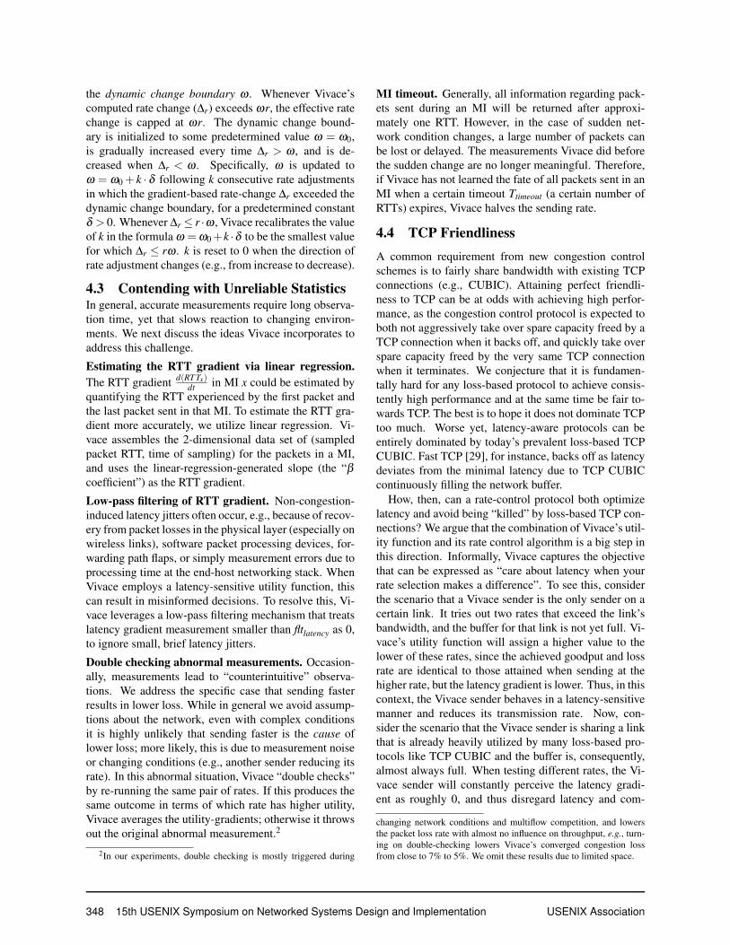
Among the evaluated protocols, BBR yields the worstTCP friendliness. In [1, 8], BBR’s TCP friendliness wasnoted to be satisfactory, based on a single BBR flowcompeting with a single CUBIC flow over a large buffer(2 BDP). We successfully reproduced this specific result(the leftmost point in the 4 Mbps/30 KB (2 BDP) BBRline of Figure 10). However, we discovered that as weadd more CUBIC flows, BBR becomes increasingly ag-gressive: it effectively treats all competing CUBIC flowsas a single “bundle” with its throughput ratio increasinglinearly with the number of CUBIC flows until about 16.Therefore, in practice, BBR can be very unfriendly whenthere are multiple competing CUBIC flows.

Though Allegro and Vivace-Loss are both loss-based,Vivace is much more agile in its reaction to competingTCP flows, especially under a shallow buffered network:its throughput ratio converges at 2.5 vs. Allegro’s 8. Inaddition, though Vivace-Loss dominates CUBIC whenthe number of concurrent flows is small, the final con-verged throughput ratio (about 5 at 2 BDP) is less thanhalf of that in BBR. In sum, though perfect TCP friend-liness is fundamentally hard, we believe that Vivace pro-vides a viable path towards adoption.

5.4 Flexible Convergence EquilibriumWith its unique utility function framework (§ 3.3), Vivaceunleashes the potential to be flexible and centrally con-trolled. To demonstrate this capability experimentally,we set up a link with 100 Mbps bandwidth, 30 ms RTT,and two competing flows. As shown in Figure 11, wecontrol the two flows’ bandwidth share by changing theirutility functions at 60s, 120s and 180s. The actual send-ing rate closely tracks the ideal allocation (dashed lines).This is only to illustrate the basic capability of Vivace;we leave a full-fledged system leveraging this capabilityto future work.

5.5 Benefits in the Real WorldIn addition to the above transport-level experiments oncontrolled networks, we test a video streaming applica-tion and performance in the wild Internet.

5.5.1 Video StreamingWe implemented a transparent proxy so that RTSP-over-TCP traffic flows from an OpenRTSP [4] client over alegacy TCP connection ending at a client-side proxy,then over a configurable transport protocol across thebottleneck link to a server-side proxy, and finally over asecond legacy TCP connection to an OpenRTSP server;similar proxying occurs in reverse. We compare thestreamed video’s buffering ratio [10], calculated as theratio of time spent during buffering relative to totalstreaming session time, using Vivace-Latency, Allegro-Latency, BBR, and TCP CUBIC. We test with four 4Kvideos, with 15 Mbps, 30 Mbps, 50 Mbps, and 95 Mbpsaverage bit rate requirements in experiments in Emulab.

We first evaluate the buffering ratio with RTT chang-ing every five seconds to a value uniform-randomly se-lected between 10 ms and 100 ms. We set up a link with300 KB buffer and 0.01% random loss rate, with the net-work bandwidth at least 10% more than the bit rate re-quired to stream the requested video. Fig. 12(a) showsthe average buffering ratio of Vivace-Latency stays be-low 8%, similar to Allegro-Latency – a reduction of atleast 86% and 90% compared with BBR and CUBIC.

To demonstrate the application-level benefit of Vi-vace’s stable convergence, we set up three competingstreaming flows from three client-server pairs. Theyshare a bottleneck link with 75 KB buffer, 100 ms RTT,0.01% random loss, and adequate bandwidth for all threeto stream. As shown in Figure 12(b), Vivace-Latencyoutperforms Allegro-Latency, BBR, and CUBIC by atleast 48%, 57%, and 80%, respectively. We attribute thedegraded performance of Allegro-Latency to its inferiorlatency awareness and reaction, and that of BBR to itshigh throughput variance among flows.

5.5.2 The Wild InternetFinally, we evaluate Vivace’s real-world performance inthe wild Internet. We set up senders at 3 different resi-dential WiFi networks and receivers at 14 Amazon WebService (AWS) sites, i.e., 42 sender-receiver pairs.5 AsWiFi networks have more noise in latency than wirednetworks, we use a slightly larger fltlatency = 0.05 to filtersmall variation of latency.6 For each AWS site we test allprotocols, and compute the average throughput of eachprotocol from five 100 sec transmissions. Figure 12(c)

5We test only the uplink because the virtualized AWS server im-pacts performance of our current user-space UDP-based packet pacing.

6We expect that in a full implementation, Vivace can automaticallyadjust fltlatency when observing high latency variance.


0

10

20

30

40

50

60

70

80

90

100

10 20 30 40 50 60 70 80 90 100

Buff

eri

ng R

ati

o (

%)

Bit Rate (Mbps)

Vivace-LatencyAllegro-LatencyBBRTCP Cubic

(a) Video streaming with varying latency

0

10

20

30

40

50

60

70

80

90

100

10 20 30 40 50 60 70 80 90 100

Buff

eri

ng R

ati

o (

%)

Bit Rate (Mbps)

Vivace-LatencyAllegro-LatencyBBRTCP Cubic

(b) Multiflow video streaming

0

20

40

60

80

100

0 5 10 15 20 25 30 35 40

Perc

enta

ge o

f Tri

als

(%

)

Average Throughput (Mbps)

Vivace-LossVivace-LatencyAllegroBBRTCP CUBIC

(c) Throughput from home networks toAWS

Figure 12: Performance gain in application and live Internet environments

shows the cumulative distribution of average through-put. Similar to the results in controlled networks, Vivace-Loss is slightly better than Vivace-Latency, and they bothoutperform BBR and CUBIC. Specifically, Vivace-Losshas a median throughput gain of 7.2%, 18.9%, and 4.0×compared with Allegro, BBR, and CUBIC, respectively.

More importantly, even though having the possibilityto be overly friendly to TCP, Vivace-Latency success-fully achieves 11.6% and 3.7× better throughput thanBBR and CUBIC in the median, i.e., CUBIC flows justcannot efficiently utilize the available bandwidth. Thisserves as a strong validation that Vivace provides a viabledeployment path, although larger scale evaluation is de-sirable. Specifically, more substantial measurements areneeded to answer the question of how Vivace behaves onreal-world traffic patterns [28].

The root cause of the difference between Vivace-Lossand Allegro is Allegro’s slow reaction to network condi-tion variation, e.g. packet loss due to available bandwidthreduction or congestion. As a result, it may gain higherthroughput occasionally (only after 90th percentile), butit will suffer from a higher loss rate and often yield moreaggressive behavior compared to Vivace.

6 Related WorkWe have already discussed Remy, and compared withseveral TCP variants, PCC Allegro, and BBR. We nextplace Vivace in the context of other related work.

In-network feedback. One class of protocols improvecongestion control by providing explicit in-networkfeedback (e.g. available bandwidth and ECN) for bet-ter informed decisions [5, 7, 20]. These protocols yieldgood performance, but have been proven to be hard todeploy outside of data centers: they require coordinatedchange of protocols and network devices. Vivace on theother hand is compatible with the TCP message format,only requires deployment at the sender, and is thereforereadily deployable.

Specially engineered congestion control. Another classof the recent works targets TCP’s poor performance inspecific network scenarios like LTE networks [32, 36]or data center networks [5, 24, 33] by leveraging unique

insights of particular networks’ behavior models, spe-cial tools or explicit feedback from the receiver. Someof these works are also moving away from TCP’s hard-wired control mechanism and are more like BBR; e.g.,Timely [24] uses the RTT-gradient as a control signalsimilar to Vivace, but it still uses a hardwired rate con-trol algorithm that maps events to fixed reactions (e.g.,using fixed thresholds and step sizes). Protocols in thisclass provide significant performance gains, but only tar-get very specific environments. Some of them also re-quire changes at both endpoints [32], which may chal-lenge deployment in practice.

Short flows. Some congestion control protocols aimto optimize performance of very short flows [22, 25].These are complementary to Vivace, because short-flowoptimization in many cases is an “open loop” problem(i.e. transfer as much data as possible in first few RTTswith very limited feedback) whereas Vivace targets the“closed loop” phase of data transfer (when meaningfulfeedback can be gathered with long enough data trans-fer). In fact Vivace could plausibly utilize [22, 25] as itsstarting phase, replacing slow-start.

7 ConclusionWe proposed Vivace, a congestion control architecturebased on online optimization theory. Vivace lever-ages a novel latency-aware utility function frameworkwith gradient-ascent-based online learning rate control toachieve provably fast convergence and fairness guaran-tees. Extensive experimentation reveals that Vivace sig-nificantly improves upon the existing state of the art interms of performance, convergence speed, reactiveness,TCP friendliness, and more. Vivace requires sender-onlychanges and is hence readily deployable. We leave re-search questions regarding centralized resource alloca-tion via Vivace’s simple interface, and Vivace’s integra-tion into comprehensive emulators such as Pantheon [35]and production systems such as QUIC [21] and the Linuxkernel, to the future.

We thank our shepherd, Alex Snoeren, and the review-ers for their helpful comments, and Google and Huaweifor ongoing support of the PCC project.


References

[1] BBR talk in IETF 97. www.ietf.org/proceedings/97/slides/slides-97-iccrg-bbr-congestion-control-01.pdf.

[2] Full Proof of Theorems. http://www.ttmeng.net/pubs/vivace_proof.pdf.

[3] Linux net-next. https : / / kernel .googlesource . com / pub / scm /linux / kernel / git / davem / net -next.git/+/v4.10.

[4] OpenRTSP. http://www.live555.com/openRTSP/.

[5] ALIZADEH, M., GREENBERG, A., MALTZ, D.,PADHYE, J., PATEL, P., PRABHAKAR, B., SEN-GUPTA, S., AND SRIDHARAN, M. Data centerTCP. Proc. of ACM SIGCOMM (September 2010).

[6] BRAKMO, L., LAWRENCE, S., O’MALLEY, S.,AND PETERSON, L. TCP Vegas: New techniquesfor congestion detection and avoidance. Proc. ofACM SIGCOMM (1994).

[7] CAESAR, M., CALDWELL, D., FEAMSTER, N.,REXFORD, J., SHAIKH, A., AND VAN DERMERWE, K. Design and implementation of a rout-ing control platform. Proc. of NSDI (April 2005).

[8] CARDWELL, N., CHENG, Y., GUNN, C.,YEGANEH, S., AND JACOBSON, V. BBR:Congestion-based congestion control. Queue 14,5 (2016), 50.

[9] CHOWDHURY, M., ZHONG, Y., AND STOICA, I.Efficient coflow scheduling with varys.

[10] DOBRIAN, F., SEKAR, V., AWAN, A., STOICA,I., JOSEPH, D., GANJAM, A., ZHAN, J., ANDZHANG, H. Understanding the impact of videoquality on user engagement. Proc. of ACM SIG-COMM (August 2011).

[11] DONG, M., LI, Q., ZARCHY, D., GODFREY,P. B., AND SCHAPIRA, M. PCC: Re-architectingCongestion Control for Consistent High Perfor-mance. Proc. of NSDI (March 2015).

[12] EVEN-DAR, M. E., MANSOUR, Y., AND NADAV,U. On the convergence of regret minimization dy-namics in concave games. Proc. of ACM sympo-sium on Theory of computing (2009).

[13] GHOBADI, M., YEGANEH, S., AND GANJALI,Y. Rethinking end-to-end congestion controlin software-defined networks. Proc. of HotNets(November 2012).

[14] GU, Y. UDT: a high performance data transportprotocol. University of Illinois at Chicago, 2005.

[15] HA, S., RHEE, I., AND XU, L. CUBIC: Anew TCP-friendly high-speed TCP variant. ACMSIGOPS Operating Systems Review (2008).

[16] HAZAN, E. Introduction to online con-vex optimization. http://ocobook.cs.princeton.edu/OCObook.pdf.

[17] HONG, C., KANDULA, S., MAHAJAN, R.,ZHANG, M., GILL, V., NANDURI, M., AND WAT-TENHOFER, R. Achieving high utilization withsoftware-driven WAN. Proc. of ACM SIGCOMM(August 2013).

[18] JAIN, S., KUMAR, A., MANDAL, S., ONG, J.,POUTIEVSKI, L., SINGH, A., VENKATA, S.,WANDERER, J., ZHOU, J., AND ZHU, M. B4:Experience with a globally-deployed software de-fined wan. ACM Computer Communication Review(September 2013).

[19] JIANG, J., SUN, S., SEKAR, V., AND ZHANG,H. Pytheas: Enabling data-driven quality of expe-rience optimization using group-based exploration-exploitation. Proc. of NSDI (March 2017).

[20] KATABI, D., HANDLEY, M., AND ROHRS, C.Congestion control for high bandwidth-delay prod-uct networks. Proc. of ACM SIGCOMM (August2002).

[21] LANGLEY, A., RIDDOCH, A., WILK, A., VI-CENTE, A., KRASIC, C., ZHANG, D., YANG, F.,KOURANOV, F., SWETT, I., IYENGAR, J., ET AL.The quic transport protocol: Design and internet-scale deployment. In Proceedings of the Confer-ence of the ACM Special Interest Group on DataCommunication (2017), ACM, pp. 183–196.

[22] LI, Q., DONG, M., AND GODFREY, P. Halfback:Running short flows quickly and safely. Proc. ofCoNEXT (November 2015).

[23] LIU, S., BASAR, T., AND SRIKANT, R. TCP-Illinois: A loss-and delay-based congestion controlalgorithm for high-speed networks. PerformanceEvaluation (2008).


[24] MITTAL, R., LAM, V. T., DUKKIPATI, N., BLEM,E. R., WASSEL, H. M. G., GHOBADI, M., VAH-DAT, A., WANG, Y., WETHERALL, D., ANDZATS, D. TIMELY: RTT-based congestion con-trol for the datacenter. In Proceedings of the2015 ACM Conference on Special Interest Groupon Data Communication, SIGCOMM 2015, Lon-don, United Kingdom, August 17-21, 2015 (2015),S. Uhlig, O. Maennel, B. Karp, and J. Padhye, Eds.,ACM, pp. 537–550.

[25] MITTAL, R., SHERRY, J., RATNASAMY, S., ANDSHENKER, S. Recursively cautious congestioncontrol. Proc. of NSDI (March 2014).

[26] NETRAVALI, R., SIVARAMAN, A., DAS, S.,GOYAL, A., WINSTEIN, K., MICKENS, J., ANDBALAKRISHNAN, H. Mahimahi: Accurate record-and-replay for HTTP. Proc. USENIX ATC (August2015).

[27] SIVARAMAN, A., WINSTEIN, K., THAKER, P.,AND BALAKRISHNAN, H. An experimental studyof the learnability of congestion control. Proc. ofACM SIGCOMM (August 2014).

[28] SUN, Y., YIN, X., JIANG, J., SEKAR, V., LIN, F.,WANG, N., LIU, T., AND SINOPOLI, B. Cs2p: Im-proving video bitrate selection and adaptation withdata-driven throughput prediction. Proc. of ACMSIGCOMM (August 2016).

[29] WEI, D., JIN, C., LOW, S., AND HEGDE, S. FASTTCP: motivation, architecture, algorithms, perfor-mance. IEEE/ACM Transactions on Networking(2006).

[30] WHITE, B., LEPREAU, J., STOLLER, L., RICCI,R., GURUPRASAD, G., NEWBOLD, M., HIBLER,M., BARB, C., AND JOGLEKAR, A. An integratedexperimental environment for distributed systemsand networks. Proc. of OSDI (December 2002).

[31] WINSTEIN, K., AND BALAKRISHNAN, H. TCP exMachina: computer-generated congestion control.Proc. of ACM SIGCOMM (August 2013).

[32] WINSTEIN, K., SIVARAMAN, A., AND BALAKR-ISHNAN, H. Stochastic forecasts achieve highthroughput and low delay over cellular networks.Proc. of NSDI (March 2013).

[33] WU, H., FENG, Z., GUO, C., AND ZHANG, Y.ICTCP: Incast congestion control for TCP in datacenter networks. Proc. of CoNEXT (November2010).

[34] XIE, X., ZHANG, X., KUMAR, S., AND LI, L. E.pistream: Physical layer informed adaptive videostreaming over lte. In Mobicom (2015).

[35] YAN, F. Y., MA, J., HILL, G., RAGHAVAN,D., WAHBY, R. S., LEVIS, P., AND WINSTEIN,K. Pantheon: the training ground for internetcongestion-control research, 2018.

[36] ZAKI, Y., POTSCH, T., CHEN, J., SUBRAMA-NIAN, L., AND GORG, C. Adaptive congestioncontrol for unpredictable cellular networks. Proc.of ACM SIGCOMM (August 2015).

[37] ZINKEVICH, M. Online convex programming andgeneralized infinitesimal gradient ascent. In ICML(2003), AAAI Press, pp. 928–936.


pcc vivace: online-learning congestion control - usenix.org · scheme. vivace adopts the high-level...

Documents