pdf - arxiv.org · pdf filepower transmission, the (modi ed) friis transmission equation...
TRANSCRIPT

Experimental Probes of Radio Wave Propagation near DielectricBoundaries and Implications for Neutrino Detection
R. Alvarez, J.C. Hanson, A.M. Johannesen, J. Macy, S. Prohira,J. Stockham, M. Stockham, Al. Zheng, and Am. Zheng
University of Kansas, Lawrence, KS 66045
D.Z. Besson and I. Bikov
National Research Nuclear University MEPhI (MoscowEngineering Physics Institute), Moscow 115409 Russia
(Dated: January 16, 2017)
AbstractExperimental efforts to measure neutrinos by radio-frequency (RF) signals resulting from neutrino
interactions in-ice have intensified over the last decade. Recent calculations indicate that one may
dramatically improve the sensitivity of ultra-high energy (“UHE”; ≥ 1018 eV) neutrino experiments
via detection of radio waves trapped along the air-ice surface. Detectors designed to observe the
“Askaryan effect” currently search for RF electromagnetic pulses propagating through bulk ice, and
could therefore gain sensitivity if signals are confined to the ice-air boundary. To test the feasibilty of this
scenario, measurements of the complex radio-frequency properties of several air-dielectric interfaces were
performed for a variety of materials. Two-dimensional surfaces of granulated fused silica (sand), both in
the lab as well as occurring naturally, water doped with varying concentrations of salt, natural rock salt
formations, granulated salt and ice itself were studied, both in North America and also Antarctica. In
no experiment do we observe unambiguous surface wave propagation, as would be evidenced by signals
traveling with reduced signal loss and/or superluminal velocities, compared to conventional EM wave
propagation. We therefore conclude that the prospects for experimental realization of such detectors
are not promising.
1
arX
iv:1
509.
0499
7v2
[as
tro-
ph.I
M]
12
Jan
2017
I. INTRODUCTION
Cosmic rays propagating towards Earth from large redshifts can produce neutrinos by in-teracting with the cosmic microwave background[1–3]. The Aksaryan effect[4] provides an at-tractive neutrino detection scheme whereby the charged and neutral current neutrino-nucleoninteractions in a dielectric material create hadronic and electromagnetic cascades that radiatecoherently in the 102 − 103 MHz bandwidth, or wavelengths in the 30-300 cm range[5]. Givenits natural abundance in pure form, ice is the most convenient dielectric material, because thelong radio attenuation length (≈2 km in the coldest ice) facilitates observation of in-ice neutrinointeractions by receivers (Rx) several km distant[6, 7].
The Antarctic ice sheet represents a unique laboratory for studies of surface effects, giventhe dielectric contrast at the air/snow interface, and the semi-infinite character of the ice sheet.Antartic ice is a remote and largely inaccessible laboratory, however, so we have conducted aseries of separate, and somewhat overlapping laboratory measurements to search for evidence ofsurface excitations. Inherent in each technique are systematic uncertainties, usually due to thefinite scale of the measurement apparatus; redundancy is therefore essential in order to derive acomposite picture. The techniques can be classified as follows:
• Measurement of signal amplitude reduction as a function of distance from a transmitter(Tx) near a dielectric boundary.
• Direct measurements of group velocities for waves propagating near a dielectric boundaryusing signal impulses (in which case direct arrival times are determined), and correspondingdetermination of the index-of-refraction.
• Measurements of phase velocity, by tracking the phase of a continuous-wave (CW) sourcepropagating near that boundary,
• Inference of index-of-refraction by measurements of the Voltage Standing Wave Ratio(VSWR) of antennas near a dielectric boundary.
We now discuss some of the studies that have been performed thus far. Most relevant to thegoals of neutrino detection are two unpublished experiments performed by the ARIANNA vs.ARA collaborations in Antarctica – the former was consistent with the observation of surfacewave excitations connecting an in-ice transmitter at a depth of 20 m to a surface receiver, over ahorizontal distance of 1000 m; the latter was similar geometrically, but with no signal detectedat a depth of 25 m from a surface transmitter over a horizontal distance of 100 m. Future workin this direction is essential in determining the viability of this approach.
II. MEASUREMENT OF ATTENUATION LENGTH DEPENDENCE ON DISTANCE
The attenuation length is typically defined with respect to the electric field (directly propor-tional to the voltage measured at the feed point of our receiver dipole antennas). In terms ofpower transmission, the (modified) Friis transmission equation states that the power receivedat the receiver after the signal has propagated a distance d through the medium with fieldattenuation length L is
Prec/Ptrans ∼GRxGTx
d2exp
(−2
d
L
). (1)
Here, G is a gain factor depending on the angular orientation of the transmitter and receiver.For two aligned dipoles, G is effectively of order unity. Applying equation 1 to two receivers
2
at distances r1 and r2 from the transmitter, we have (in a three-dimensional material), for thevoltages V1 and V2 measured at the two points:
V2/V1 =r1
r2
exp (−(r2 − r1)/L) (2)
Equation 2 assumes that P ∝ V 2, and that the antennas are linear devices with a constanteffective height converting electric fields into voltages (a standard property of dipole antennas,e.g.). Comparing an antenna measurement in air (with no appreciable attenuation) to thedielectric material, equation 2 becomes
Vdiel/Vair =rairrdiel
exp (−(rdiel − rair)/L) (3)
In our case, we seek to investigate ‘trapping’ of electric field flux within a boundary surfacelayer. In such a case, the dependence of signal power with distance falls more slowly than forflux spreading into the bulk (1/r vs. 1/r2), suggesting significantly more advantageous neutrinodetection efficiency for near-surface radio receivers rather than englacial radio receivers.
A. Laboratory Amplitude Measurements in Sand
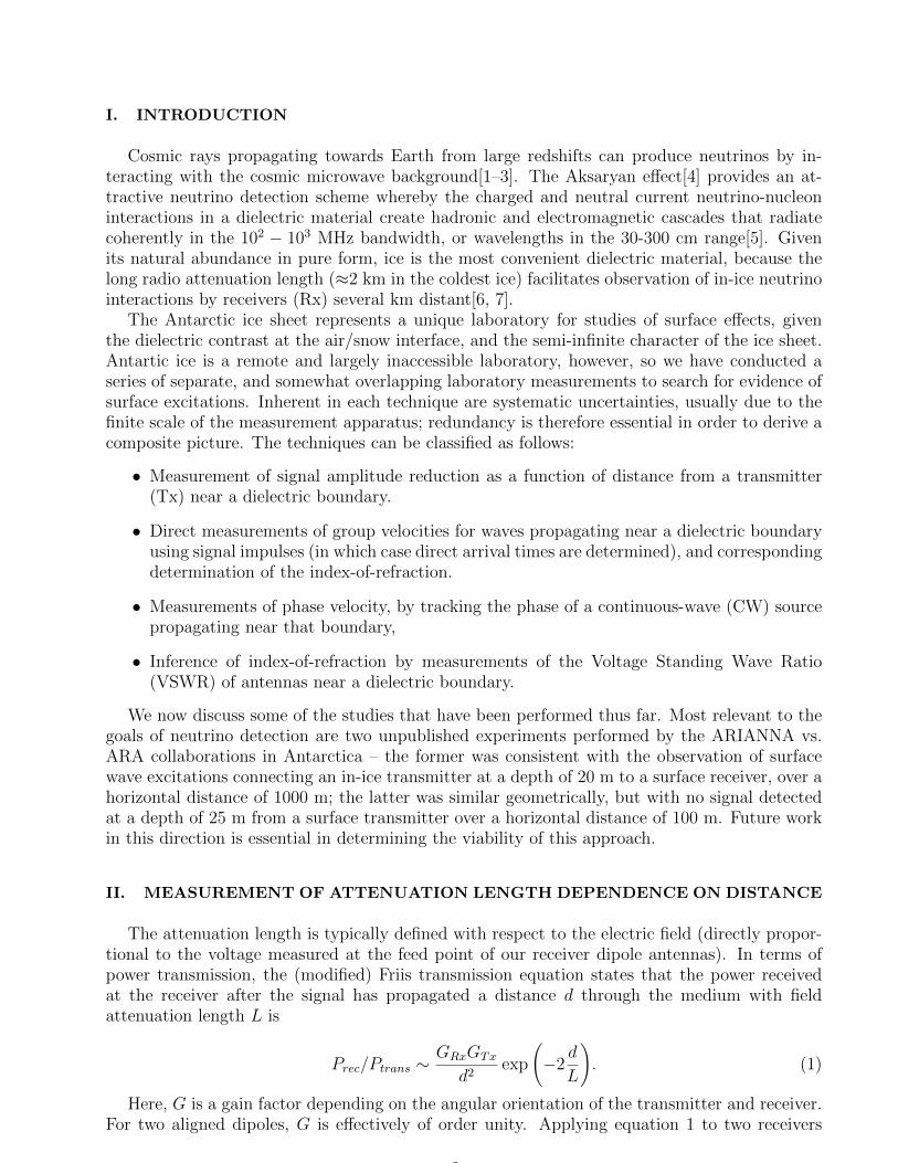
On the University of Kansas campus, we have attempted to discern surface wave effects usingthe sand volleyball courts located at the University’s gym and recreational facilities. Thesehave the advantage of close proximity to the KU Physics Department, but the disadvantage oflimited depth (typically 30 cm of dry sand, followed by a deeper layer susceptible to increasingmoisture). Our measurements consisted of a series of peak voltages for impulses, measured as afunction of separation distance between transmitter and receiver; for these measurements, bothtransmitter and receiver were half-buried in the sand. Each of the 5 cm diameter, 30 cm longRICE[22] neutrino detection experiment’s half-wave “fat” dipole antennas offers good receptionover the range 0.2–1 GHz. The peak response of the antenna is measured to be at ∼450 MHzin air (or 450 MHz/n in a medium characterized by index-of-refraction n) with a fractionalbandwidth ∆f
f∼0.2. Figure 1 shows the result of this exercise. Although the data quality are
reasonably good and favor the 1/r fit, we cannot conclusively discriminate between V (r) ∝ 1/rvs. V (r) ∝ 1/
√r, corresponding to spherical vs. planar flux-spreading, respectively.
B. Amplitude Measurements at South Pole with the RICE Experiment
As an alternative, we have attempted to quantify planar signal flux trapping directly fromdata taken using a fat dipole antenna transmitter/receiver pair lowered into two neighboringiceholes drilled for the RICE experiment at the South Pole in 1998. Each of these mechanicallyholes is approximately 180 m deep and 12 cm in diameter.
Two different trials were carried out in the original experiment, conducted in 2003, which wehave recently re-analyzed. That experiment targeted a measurement of the index-of-refractiondependence with depth, rather than measurement of surface waves, so control of systematics weredesigned with the former goal in mind. In each trial, two antennas were placed near-surface,and the propagation time, as well as the signal voltage registered at the receiver recorded.Next, the two antennas were co-lowered into parallel iceholes with a horizontal separation oforder 50 m. Of interest here is the signal amplitude after the antennas have descended severalwavelengths into the ice, at which point the received signal voltage can be compared with thenear-surface measurements. If signal has been trapped in the boundary layer in the lattercase, then, given the negligible radio-frequency signal absorption in the near-surface ice firn,
3
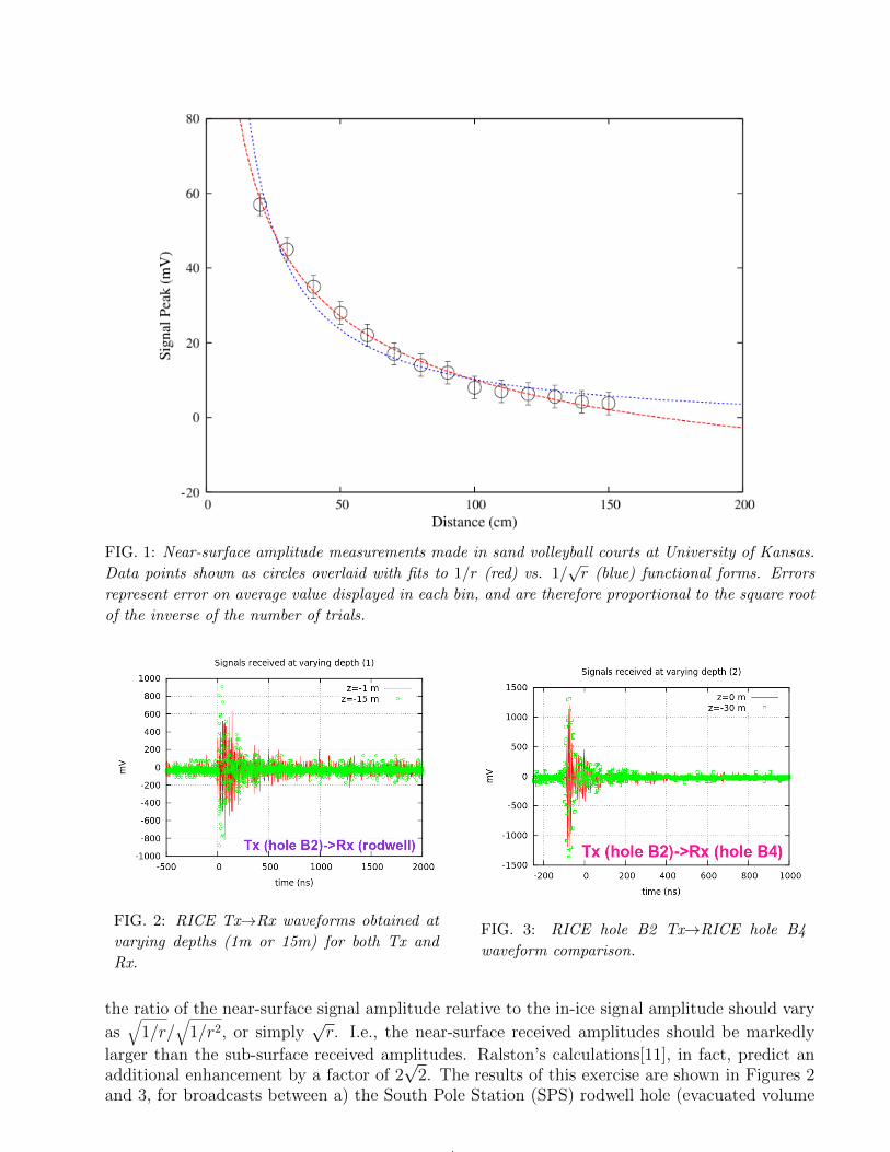
FIG. 1: Near-surface amplitude measurements made in sand volleyball courts at University of Kansas.
Data points shown as circles overlaid with fits to 1/r (red) vs. 1/√r (blue) functional forms. Errors
represent error on average value displayed in each bin, and are therefore proportional to the square root
of the inverse of the number of trials.
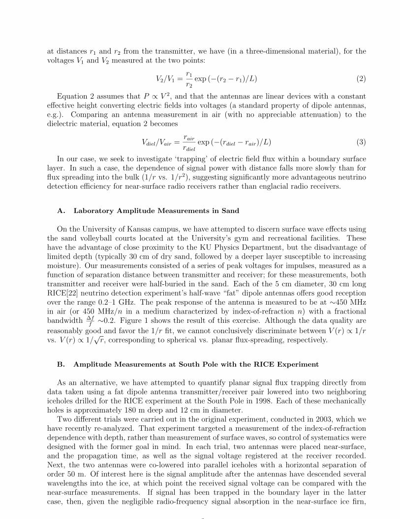
FIG. 2: RICE Tx→Rx waveforms obtained at
varying depths (1m or 15m) for both Tx and
Rx.
FIG. 3: RICE hole B2 Tx→RICE hole B4
waveform comparison.
the ratio of the near-surface signal amplitude relative to the in-ice signal amplitude should vary
as√
1/r/√
1/r2, or simply√r. I.e., the near-surface received amplitudes should be markedly
larger than the sub-surface received amplitudes. Ralston’s calculations[11], in fact, predict anadditional enhancement by a factor of 2
√2. The results of this exercise are shown in Figures 2
and 3, for broadcasts between a) the South Pole Station (SPS) rodwell hole (evacuated volume
4

remaining after melted ice has been extracted for general SPS use) and RICE hole B2 and b)RICE hole B2 and RICE hole B4, respectively. Although there is some moderate change in thewaveform shapes of the near-surface vs. the deep-ice received signals, the overall received powerin the first ∼100 ns of the initial pulse emission is comparable in the in-ice vs. the near-surfacetransmission cases, and inconsistent with the expected enhancement by a factor of >
√50 m
that would be expected for the case of surface signal flux trapping.
C. Check of Surface Confinement using a Snow ‘Barrier’
Although not fully examined in the original theoretical work, it is interesting to investigatethe possibility that flux may be confined along a contoured surface. At South Pole, an additionalcheck was performed wherein the signal received between two horn transmitters, separated by675 m and facing each other on the snow surface was compared. In the first configuration, thetwo horn antennas had clear line-of-sight (LOS) relative to each other; in that configuration,the receiver antenna registered signals at Signal-to-Noise Ratio (SNR) levels, in units of therms noise voltage σthermal, of 12σthermal and 14σthermal for the HPol and VPol configurations,respectively. In the second configuration, although the separation distance remained at 675 m,the transmitter was displaced horizontally approximately 100 meters, to a location where thesnow surface was approximately 4 meters lower compared to the original location, such thatthere was no longer LOS to the receiver. In that second case, we observe no signal above noise,ruling out the possibility that a surface wave is following the contour of the surface between thetransmitter source and the receiver.
D. Amplitude Measurements at South Pole with the ARA Experiment
A successor to RICE, the South Polar Askaryan Radio Array[23] (ARA) neutrino detectionexperiment similarly consists of an array of radio receivers deployed both on the surface, as wellas in several boreholes, separated by ∼20 m horizontally, with each hole containing 3–4 verticallystacked receiver antennas, separated by 5–10 m in the bulk ice. ARA has, thus far, developed inthree stages: a) deployment of a prototype (‘testbed’) in January, 2011, consisting of 2 surfaceantennas sensitive over the frequency range f < 200 MHz, 4 near-surface antennas deployed inthe upper meter of Antarctic ice sensitive over 150 MHz< f <900 MHz, plus 10 antennas (150MHz< f <900 MHz) deployed between 30 and 24 meters beneath the surface, b) deploymentof the ARA1 station in January, 2012, including 4 surface antennas, and using optical fiber toconvey signals from the 16 ∼90-m deep in-ice antennas to the surface, and c) deployment of theARA2 and ARA3 stations in January, 2013, based on the ARA1 model, but with a deeper in-iceantenna deployment, to a depth of 180–200 meters.
Of these, the testbed data are most informative for surface wave studies. Calibration con-tinuous wave (CW) data were taken in the testbed receiver array in December, 2011, from twodifferent transmitter configurations: a) RICE dipole transmitter buried just sub-surface (z=–25cm) at a radial distance 100 m from the center of the testbed array, and b) the same dipoletransmitter elevated 1 meter above the surface. For both of these cases, ARA receiver data weretaken at 90-degree angular increments, in order to average over possible azimuthal Tx or Rxasymmetries.
For configuration a), both HPol and VPol data are shown, as a function of transmitterfrequency, broadcast in 100 MHz increments, in Figures 4 and 5. Shown is the ratio of peaksignal amplitude in the frequency domain (after performing a Fourier transform on the time-domain captured waveforms), averaged over the 4 compass-point Tx source locations for whichdata were taken. To examine possible surface wave effects, and to remove possible transmitter
5
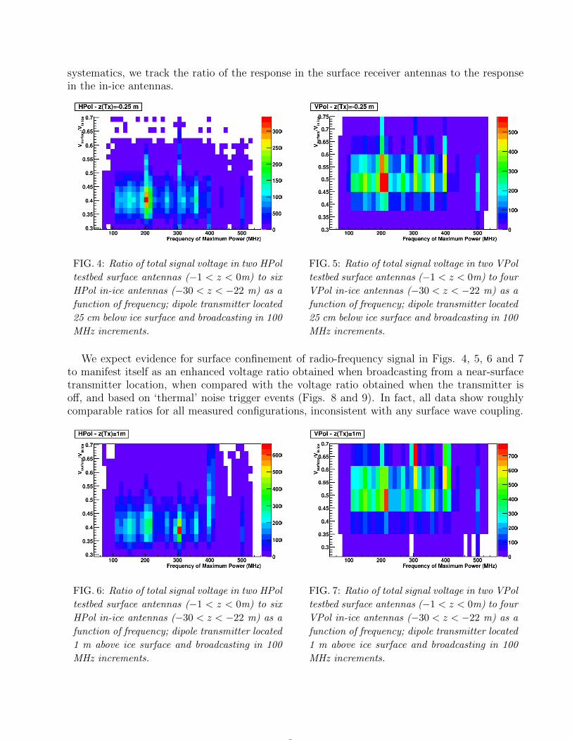
systematics, we track the ratio of the response in the surface receiver antennas to the responsein the in-ice antennas.
FIG. 4: Ratio of total signal voltage in two HPol
testbed surface antennas (−1 < z < 0m) to six
HPol in-ice antennas (−30 < z < −22 m) as a
function of frequency; dipole transmitter located
25 cm below ice surface and broadcasting in 100
MHz increments.
FIG. 5: Ratio of total signal voltage in two VPol
testbed surface antennas (−1 < z < 0m) to four
VPol in-ice antennas (−30 < z < −22 m) as a
function of frequency; dipole transmitter located
25 cm below ice surface and broadcasting in 100
MHz increments.
We expect evidence for surface confinement of radio-frequency signal in Figs. 4, 5, 6 and 7to manifest itself as an enhanced voltage ratio obtained when broadcasting from a near-surfacetransmitter location, when compared with the voltage ratio obtained when the transmitter isoff, and based on ‘thermal’ noise trigger events (Figs. 8 and 9). In fact, all data show roughlycomparable ratios for all measured configurations, inconsistent with any surface wave coupling.
FIG. 6: Ratio of total signal voltage in two HPol
testbed surface antennas (−1 < z < 0m) to six
HPol in-ice antennas (−30 < z < −22 m) as a
function of frequency; dipole transmitter located
1 m above ice surface and broadcasting in 100
MHz increments.
FIG. 7: Ratio of total signal voltage in two VPol
testbed surface antennas (−1 < z < 0m) to four
VPol in-ice antennas (−30 < z < −22 m) as a
function of frequency; dipole transmitter located
1 m above ice surface and broadcasting in 100
MHz increments.
6
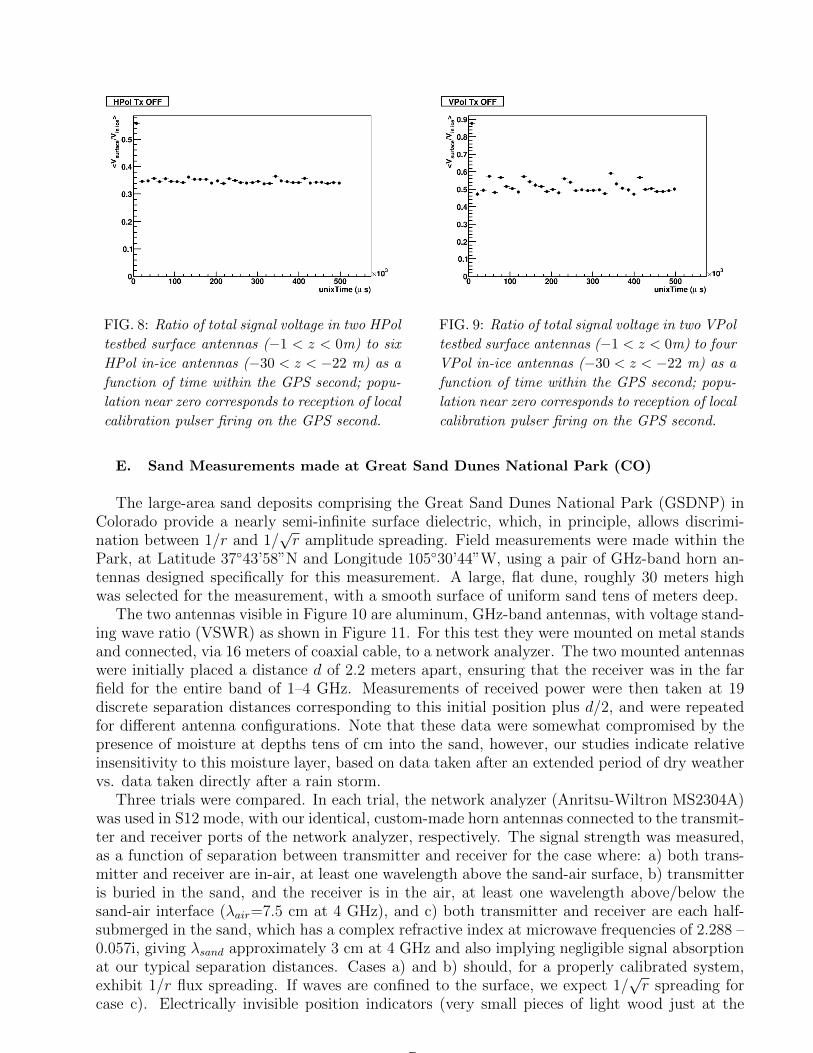
FIG. 8: Ratio of total signal voltage in two HPol
testbed surface antennas (−1 < z < 0m) to six
HPol in-ice antennas (−30 < z < −22 m) as a
function of time within the GPS second; popu-
lation near zero corresponds to reception of local
calibration pulser firing on the GPS second.
FIG. 9: Ratio of total signal voltage in two VPol
testbed surface antennas (−1 < z < 0m) to four
VPol in-ice antennas (−30 < z < −22 m) as a
function of time within the GPS second; popu-
lation near zero corresponds to reception of local
calibration pulser firing on the GPS second.
E. Sand Measurements made at Great Sand Dunes National Park (CO)
The large-area sand deposits comprising the Great Sand Dunes National Park (GSDNP) inColorado provide a nearly semi-infinite surface dielectric, which, in principle, allows discrimi-nation between 1/r and 1/
√r amplitude spreading. Field measurements were made within the
Park, at Latitude 37◦43’58”N and Longitude 105◦30’44”W, using a pair of GHz-band horn an-tennas designed specifically for this measurement. A large, flat dune, roughly 30 meters highwas selected for the measurement, with a smooth surface of uniform sand tens of meters deep.
The two antennas visible in Figure 10 are aluminum, GHz-band antennas, with voltage stand-ing wave ratio (VSWR) as shown in Figure 11. For this test they were mounted on metal standsand connected, via 16 meters of coaxial cable, to a network analyzer. The two mounted antennaswere initially placed a distance d of 2.2 meters apart, ensuring that the receiver was in the farfield for the entire band of 1–4 GHz. Measurements of received power were then taken at 19discrete separation distances corresponding to this initial position plus d/2, and were repeatedfor different antenna configurations. Note that these data were somewhat compromised by thepresence of moisture at depths tens of cm into the sand, however, our studies indicate relativeinsensitivity to this moisture layer, based on data taken after an extended period of dry weathervs. data taken directly after a rain storm.
Three trials were compared. In each trial, the network analyzer (Anritsu-Wiltron MS2304A)was used in S12 mode, with our identical, custom-made horn antennas connected to the transmit-ter and receiver ports of the network analyzer, respectively. The signal strength was measured,as a function of separation between transmitter and receiver for the case where: a) both trans-mitter and receiver are in-air, at least one wavelength above the sand-air surface, b) transmitteris buried in the sand, and the receiver is in the air, at least one wavelength above/below thesand-air interface (λair=7.5 cm at 4 GHz), and c) both transmitter and receiver are each half-submerged in the sand, which has a complex refractive index at microwave frequencies of 2.288 –0.057i, giving λsand approximately 3 cm at 4 GHz and also implying negligible signal absorptionat our typical separation distances. Cases a) and b) should, for a properly calibrated system,exhibit 1/r flux spreading. If waves are confined to the surface, we expect 1/
√r spreading for
case c). Electrically invisible position indicators (very small pieces of light wood just at the
7

FIG. 10: Photograph of the two horn antennas used at the Great Sand Dunes National Park in their
“free-space” configuration.
FIG. 11: Measured Voltage-Standing Wave Ratio (VSWR) for horn antennas used in the GSDNP
experiment.
surface of the sand) were placed out 20 cm out of the specular beam path, as shown in Figure12.
8

FIG. 12: The two horn antennas used for the Great Sand Dunes National Park experiment, in a near-
surface setup.
1. Free Space
The first measurement taken was a free space test, to verify the expected flux spreading inthree-dimensions. The antennas were placed at a height of 2 m, as shown in Figure 10, greatlyreducing the influence of the sand surface on the measurement. The results of this test forseveral frequency bins are shown in Figure 13, with a fit to 1/r overlaid. We observe excellentagreement with the 1/r hypothesis.
FIG. 13: Fit to the free-space data with overlay to 1/r functional form.
9

2. Surface Measurements
The remainder of the measurements were taken to probe the possibility of exciting surfacewaves. The transmitter and receiver were set at different heights, including i) sitting on thesurface, and in contact with the surface, ii) half-buried, iii) fully-buried, or iv) elevated at leastone wavelength above the surface. A complete compilation of our obtained data are shown inFigure 14; a direct comparison of the half-buried data with free space are shown in 15. Overall,there was no significant observed difference, besides a reduction in overall amplitude (whichwe attribute to the Fresnel transmission coefficient through the air-sand interface) between thefree space case and the case where the transmitter was fully buried and the receiver was placed1 m off the surface. We can fit our measured amplitude points to the form 1/rb. The case of
FIG. 14: A comparison of several measurements. Note that the noise floor of the Network Analyzer is
approximately –65 dB; there are therefore non-negligible contributions to the observed received signal up
to ∼ −60 dB
both transmitter and receiver half-buried shows an amplitude falloff which favors 1/r over 1/√r,
although it should be noted that this measurement is close to the noise floor, particularly fordistances greater than 8 m. separations; we have correspondingly restricted the fit to the first8 points in Figure 15. The exponent obtained in Fig. 15, for example, increases towards 0.9 aswe reduce the number of fitted points, albeit with larger error bars.
III. STUDIES OF THE REAL PART OF THE PERMITTIVITY
As discussed previously, it has been suggested that surface waves may travel with a velocity(both vg and also vp) corresponding to n < 1. We have therefore searched for apparently super-luminal signal velocities. To directly measure the index-of-refraction at dielectric boundaries, aradio-frequency continuous wave (CW) signal was generated using a Rhode and Schwarz SMHUsignal generator (0.1 to 4320 MHz) with the 19 dBmW output connected to an 8 cm, 14 gaugecopper half-wavelength dipole antenna, via a 2 m (CableWave) N-connectorized coaxial cablesoldered to the antenna feed point. By measuring signals from a stationary and moving receiver,the phase at distances corresponding to half-integer multiples of the observed wavelength (λ)were recorded, yielding the effective phase velocity index-of-refraction (n = c/fλ). The receiving
10

FIG. 15: Great Sand Dunes National Park test of surface wave coupling: comparison of free space
versus tx buried, rx 1m in height.
dipoles were soldered to 3 m coaxial cables and connected to a Tektronix TDS 5104 oscilloscope.In addition to varying the distance between the two receivers, the height of both receivers abovethe surface was varied. As outlined above, distances between the two receivers corresponding toboth 0◦ and 180◦ phase shifts were recorded.
This procedure was repeated several times over the length of the dielectric medium to min-imize statistical fluctuations. The two-dimensional surface materials tested were water, waterdoped with pool salt to varying salinities, granulated fused silica (sand), and granulated sodiumchloride (salt). CW signal frequencies between 750 and 1500 MHz were investigated, each fre-quency being within the efficient transmission region of the antennas. A box to contain thedielectric media (except for the doped water) was constructed with 8.9 cm x 61 cm x 122 cmdimensions. Sand measurements from 150–500 MHz were also performed in an outdoor sandpit (c.f. Fig. 28) with the lower-frequency RICE dipole antennas[22]. The purified water wascontained within a circular pool roughly 3 m in diameter, and the salinity was recorded on anExTech EC400 conductivity/TDS/salinity meter. The technique is summarized in Figure 16.
A. Laboratory Wave Speed Measurements with Sand and Salt
Antenna orientations were sorted into the categories of in, surface, air, and half. The inlabel indicates antenna placement fully within the dense dielectric, half indicates halfway withinthe dense dielectric, surface indicates placement directly on top of the dense dielectric, and airindicates antenna placement one antenna-length above the dense dielectric. A single antennaplacement descriptor indicates all antennas were in the same position with respect to the surface,and ordered placement descriptors describe antenna position in propagation order (transmitter,static receiver, and moveable receiver, respectively). The label w/metal indicates sand dopedwith a 10:1 ratio of sand to aluminum shavings. In Figures 17-20, the x-axis indicates themeasurement trial number, corresponding to the phase position (in units of wavelengths) of themoving receiver. As that receiver was translated farther from the static receiver, the distance toeach phase position was recorded, and the phase velocity index-of-refraction derived.
Figure 17 displays the refractive index results at a frequency of 1000 MHz; results are also
11
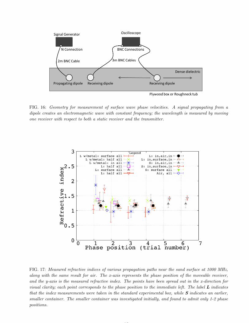
FIG. 16: Geometry for measurement of surface wave phase velocities. A signal propagating from a
dipole creates an electromagnetic wave with constant frequency; the wavelength is measured by moving
one receiver with respect to both a static receiver and the transmitter.
FIG. 17: Measured refractive indices of various propagation paths near the sand surface at 1000 MHz,
along with the same result for air. The x-axis represents the phase position of the moveable receiver,
and the y-axis is the measured refractive index. The points have been spread out in the x-direction for
visual clarity; each point corresponds to the phase position to the immediate left. The label L indicates
that the index measurements were taken in the standard experimental box, while S indicates an earlier,
smaller container. The smaller container was investigated initially, and found to admit only 1-2 phase
positions.
12

Sub-category average± error in mean
All-measurements 1.22± 0.03
Metal-doped 1.17± 0.08
Metal-doped (excl. half) 1.1± 0.1
Excl. metal-doped 1.24± 0.03
Air 1.01± 0.03
TABLE I: Summary of the average measured index-of-refraction for sand, from laboratory studies per-
formed at 1000 MHz. Errors shown are statistical only.
summarized in Table I. All combinations of signal path are shown, with mean values frommultiple trials presented along with one standard deviation statistical errors. For laboratorymeasurements, Quikrete commercial sand (No. 1962) was used. Although the sand used in theoutdoor sand pit (described below) was not commercial, the density is observed to be roughlythe same. Notice from Fig. 17 that measurements having differing antenna orientations, but forthe same phase position are statistically consistent. Measurements were made out to the highestpossible phase position before noise on the oscilloscope began to dominate the signals. Figure17 contains both data from the initial smaller set up (S) and the larger one (L). The averageindex-of-refraction for all measurements is 1.22 ± 0.03. Considering only measurements withaluminum-doped sand, the average is 1.17± 0.08. Excluding from this subset the half position,the modified average is 1.1 ± 0.1. Excluding the metal-doped measurements from the globalaverage yields < n >= 1.24 ± 0.03. The index-of-refraction of dry sand is ≈ 1.6[24], whereasair has an index of 1.0. Thus, the data suggest that the waves sample the average of the twopropagation media, consistent with the fact that one wavelength is of order or larger than theseparation between an antenna and the dielectric surface. Table I summarizes the sub-categoriesof refractive index. All measurements give index-of-refraction values intermediate between airand sand.
Figure 18 displays the refractive index results at a frequency of 1500 MHz, with the samelabeling conventions as Fig. 17. All tested combinations of signal path are shown, with measure-ments made out to the highest possible phase position. Relative to the measurements performedat 1000 MHz, the results at 1500 MHz seem to indicate increased sensitivity to the orientationof the transmitters and receivers, consistent with the expectation that, for smaller wavelengths,we are increasingly probing smaller-scale non-uniformities. Figure 18 contains both data fromthe initial smaller set up (S) and also the larger one (L). The data corresponding to submergedtransmitters and receivers (In) produce an index closer to that of air, while an all-measurementaverage and an average of just the large box data are both consistent with the results at 1000MHz. Table II summarizes the results in Fig. 18.
The experimental procedure using a moveable and a static receiving antenna was repeated inthe smaller version of the box, filled with Morton 100% NaCl rock salt, with results shown inFigures 19 and 20. Several measurements of the index-of-refraction of natural rock salt yieldedvalues between 2.4 and 2.8[25, 26] for the 100-1000 MHz regime, depending on frequency andthe rock salt purity. For this experiment, the size of the salt container limited the analysis toonly the first phase position. Additionally, the rock salt crystals changed the outline of therelatively small dipole antennas, limiting the number of orientations tested. As expected, theaverage measured index-of-refraction is higher than for the case of sand, given the known largerbulk index-of-refraction for NaCl compared to SiO2.
13

FIG. 18: The measured refractive indices for various propagation paths through sand at 1500 MHz,
along with the same result for air. The x-axis represents the phase position of the dynamic receiver,
and the y-axis is the measured refractive index. The points have been spread out in the x-direction for
visual clarity; as before, each point corresponds to the phase position to the immediate left.
Sub-category average±error in mean
All-measurements 1.20± 0.03
In, only 1.09± 0.03
All (excl. In) 1.28± 0.02
Small box only 1.447± 0.005
Large box only 1.17± 0.03
Air 1.0± 0.1
TABLE II: A summary of the average index-of-refraction measurements for sand, from the laboratory
studies performed at 1500 MHz. Errors shown are statistical only.
Sub-category average±error in mean
All measurements 1.50± 0.01
Air 1.0± 0.03
TABLE III: Summary of the average measured index-of-refraction for salt, from laboratory studies
performed at 1000 MHz. Errors shown are statistical only.
14

FIG. 19: The refractive indices for various propagation paths through salt at 1000 MHz. Only the first
phase position was tested (x-axis); the y-axis is the measured refractive index. A free-space measurement
was performed as a cross-check (square point), yielding a value consistent with 1, as expected.
FIG. 20: The measured refractive indices of various propagation paths through salt at 1500 MHz. Only
the first phase position was tested (x-axis); y-axis is the measured index-of-refraction. A free-space
measurement was performed as a cross-check (the square point). Errors shown are statistical only.
15
Sub-category average±error in mean
All measurements 1.45± 0.01
Air 1.0± 0.2
TABLE IV: Summary of the measured average index-of-refraction for salt, from laboratory studies
performed at 1500 MHz. Errors shown are statistical only.
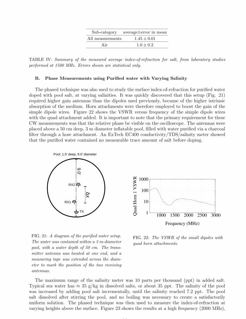
B. Phase Measurements using Purified water with Varying Salinity
The phased technique was also used to study the surface index-of-refraction for purified waterdoped with pool salt, at varying salinities. It was quickly discovered that this setup (Fig. 21)required higher gain antennas than the dipoles used previously, because of the higher intrinsicabsorption of the medium. Horn attachments were therefore employed to boost the gain of thesimple dipole wires. Figure 22 shows the VSWR versus frequency of the simple dipole wireswith the quad attachment added. It is important to note that the primary requirement for theseCW measurements was that the relative phase be visible on the oscilloscope. The antennas wereplaced above a 50 cm deep, 3 m diameter inflatable pool, filled with water purified via a charcoalfilter through a hose attachment. An ExTech EC400 conductivity/TDS/salinity meter showedthat the purified water contained no measurable trace amount of salt before doping.
9.0'
Δx
RX2
RX1
TX
Pool: 1.5' deep, 9.0' diameter
FIG. 21: A diagram of the purified water setup.
The water was contained within a 3 m-diameter
pool, with a water depth of 50 cm. The trans-
mitter antenna was located at one end, and a
measuring tape was extended across the diam-
eter to mark the position of the two receiving
antennas.
1
10
100
1000
1000 1500 2000 2500 3000Qu
ad H
orn
1 V
SW
R
Frequency (MHz)
FIG. 22: The VSWR of the small dipoles with
quad horn attachments.
The maximum range of the salinity meter was 10 parts per thousand (ppt) in added salt.Typical sea water has ≈ 35 g/kg in dissolved salts, or about 35 ppt. The salinity of the poolwas increased by adding pool salt incrementally, until the salinity reached 7.2 ppt. The poolsalt dissolved after stirring the pool, and no boiling was necessary to create a satisfactorilyuniform solution. The phased technique was then used to measure the index-of-refraction atvarying heights above the surface. Figure 23 shows the results at a high frequency (2000 MHz),
16
0.6
0.7
0.8
0.9
1
1.1
1.2
0.5 1 1.5 2 2.5 3 3.5
Ind
ex
of
Refr
acti
on
h/λ
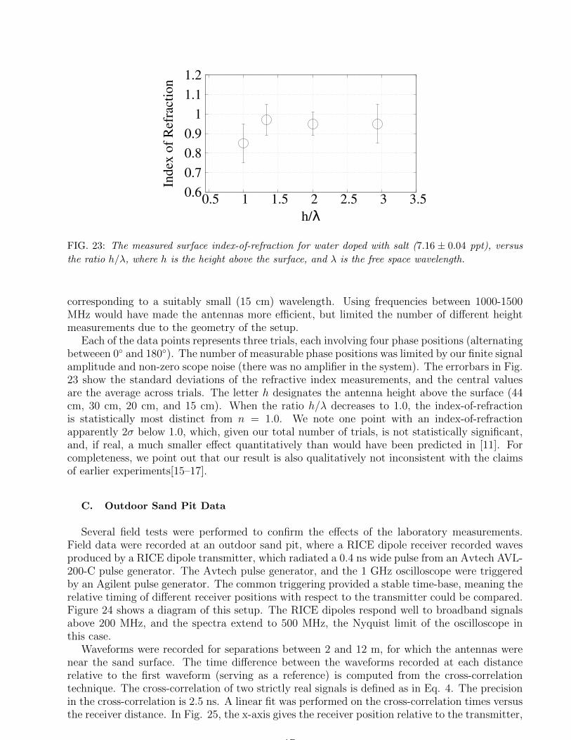
FIG. 23: The measured surface index-of-refraction for water doped with salt (7.16 ± 0.04 ppt), versus
the ratio h/λ, where h is the height above the surface, and λ is the free space wavelength.
corresponding to a suitably small (15 cm) wavelength. Using frequencies between 1000-1500MHz would have made the antennas more efficient, but limited the number of different heightmeasurements due to the geometry of the setup.
Each of the data points represents three trials, each involving four phase positions (alternatingbetweeen 0◦ and 180◦). The number of measurable phase positions was limited by our finite signalamplitude and non-zero scope noise (there was no amplifier in the system). The errorbars in Fig.23 show the standard deviations of the refractive index measurements, and the central valuesare the average across trials. The letter h designates the antenna height above the surface (44cm, 30 cm, 20 cm, and 15 cm). When the ratio h/λ decreases to 1.0, the index-of-refractionis statistically most distinct from n = 1.0. We note one point with an index-of-refractionapparently 2σ below 1.0, which, given our total number of trials, is not statistically significant,and, if real, a much smaller effect quantitatively than would have been predicted in [11]. Forcompleteness, we point out that our result is also qualitatively not inconsistent with the claimsof earlier experiments[15–17].
C. Outdoor Sand Pit Data
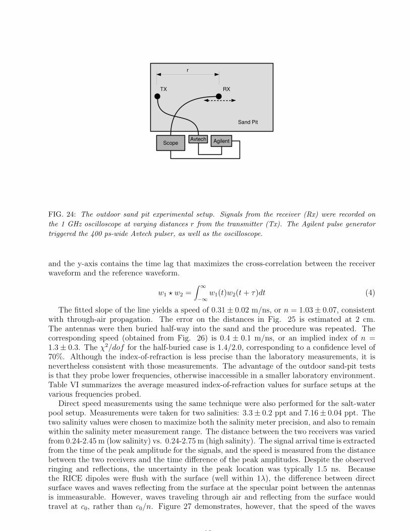
Several field tests were performed to confirm the effects of the laboratory measurements.Field data were recorded at an outdoor sand pit, where a RICE dipole receiver recorded wavesproduced by a RICE dipole transmitter, which radiated a 0.4 ns wide pulse from an Avtech AVL-200-C pulse generator. The Avtech pulse generator, and the 1 GHz oscilloscope were triggeredby an Agilent pulse generator. The common triggering provided a stable time-base, meaning therelative timing of different receiver positions with respect to the transmitter could be compared.Figure 24 shows a diagram of this setup. The RICE dipoles respond well to broadband signalsabove 200 MHz, and the spectra extend to 500 MHz, the Nyquist limit of the oscilloscope inthis case.
Waveforms were recorded for separations between 2 and 12 m, for which the antennas werenear the sand surface. The time difference between the waveforms recorded at each distancerelative to the first waveform (serving as a reference) is computed from the cross-correlationtechnique. The cross-correlation of two strictly real signals is defined as in Eq. 4. The precisionin the cross-correlation is 2.5 ns. A linear fit was performed on the cross-correlation times versusthe receiver distance. In Fig. 25, the x-axis gives the receiver position relative to the transmitter,
17
TX RX
Sand Pit
ScopeAvtech Agilent
r
FIG. 24: The outdoor sand pit experimental setup. Signals from the receiver (Rx) were recorded on
the 1 GHz oscilloscope at varying distances r from the transmitter (Tx). The Agilent pulse generator
triggered the 400 ps-wide Avtech pulser, as well as the oscilloscope.
and the y-axis contains the time lag that maximizes the cross-correlation between the receiverwaveform and the reference waveform.
w1 ? w2 =∫ ∞−∞
w1(t)w2(t+ τ)dt (4)
The fitted slope of the line yields a speed of 0.31± 0.02 m/ns, or n = 1.03± 0.07, consistentwith through-air propagation. The error on the distances in Fig. 25 is estimated at 2 cm.The antennas were then buried half-way into the sand and the procedure was repeated. Thecorresponding speed (obtained from Fig. 26) is 0.4 ± 0.1 m/ns, or an implied index of n =1.3± 0.3. The χ2/dof for the half-buried case is 1.4/2.0, corresponding to a confidence level of70%. Although the index-of-refraction is less precise than the laboratory measurements, it isnevertheless consistent with those measurements. The advantage of the outdoor sand-pit testsis that they probe lower frequencies, otherwise inaccessible in a smaller laboratory environment.Table VI summarizes the average measured index-of-refraction values for surface setups at thevarious frequencies probed.
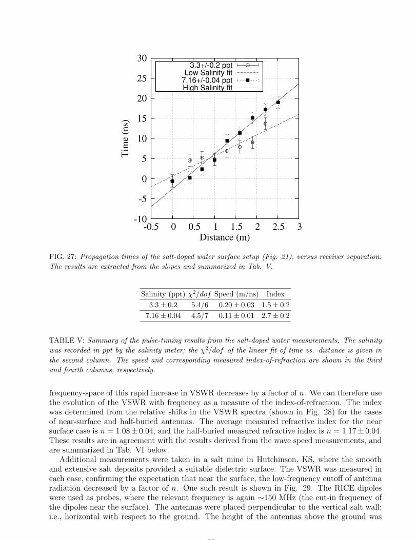
Direct speed measurements using the same technique were also performed for the salt-waterpool setup. Measurements were taken for two salinities: 3.3± 0.2 ppt and 7.16± 0.04 ppt. Thetwo salinity values were chosen to maximize both the salinity meter precision, and also to remainwithin the salinity meter measurement range. The distance between the two receivers was variedfrom 0.24-2.45 m (low salinity) vs. 0.24-2.75 m (high salinity). The signal arrival time is extractedfrom the time of the peak amplitude for the signals, and the speed is measured from the distancebetween the two receivers and the time difference of the peak amplitudes. Despite the observedringing and reflections, the uncertainty in the peak location was typically 1.5 ns. Becausethe RICE dipoles were flush with the surface (well within 1λ), the difference between directsurface waves and waves reflecting from the surface at the specular point between the antennasis immeasurable. However, waves traveling through air and reflecting from the surface wouldtravel at c0, rather than c0/n. Figure 27 demonstrates, however, that the speed of the waves
18

0
10
20
30
40
0 2 4 6 8 10 12 14
Tim
e (
ns)
Distance (m)
FIG. 25: Cross-correlation times of the sand-
pit surface setup (Fig. 24), versus receiver po-
sition. The χ2/dof is 6.3/7.0, and the inverse
of the fitted slope corresponds to the speed of the
pulses in the system. The y-intercept is consis-
tent with zero, within errors.
0
5
10
15
20
25
30
0 2 4 6 8 10 12 14
Tim
e (
ns)
Distance (m)
FIG. 26: Cross-correlation times of the sand-
pit surface setup (Fig. 24), versus receiver po-
sition, with the transmitter and receiver half-
buried. χ2/dof=1.4/2.0; y-intercept is consis-
tent with zero within errors.
in both the low and high salinity cases was less than c0. The time between antenna channelsis plotted versus channel separation, and the inverse of the slopes yields the speed. The lowsalinity data corresponds to a wave speed v = 0.20± 0.03 m/ns, and the high salinity data givesv = 0.11 ± 0.01 m/ns, with the higher index-of-refraction corresponding to the higher salinitydata. The broadband measurements show some variation relative to the CW measurements at2000 MHz, which indicated indices consistent with 1.0. Table V summarizes the fits, speed andindex measurements.
We observe contrasting trends in the salinity and sand data. The CW data originating fromsand doped with metal shavings has significantly lower index than the other subsets of results.The CW salt water and metal doped sand data show similar numbers for the index (near 1.0),indicating the geometry and conductivity of the setup plays a significant role. However, thedirect wave-speed measurements from broadband pulses yield larger numbers for the index.This suggests there may be some frequency dependence in the index-of-refraction along thesurface. Both data and modeling above 1 GHz suggest that there is already dispersive behaviorof the permittivity of water with dissolved ions[27]. The authors of that reference claim that theindex is inversely proportional to salinity. Our salinities are lower than those in Fig. 1 of[27] bya factor of 3-10, but our index measurements are also lower. We attribute this finding to thesurface geometry, versus the bulk data used to create their Fig. 1. However, since no significantsuper-luminal measurements are reported (other than the left-most point of Fig. 23, which couldbe a chance coindidence) it is not likely that these are the classical surface waves sought for inour tests.
D. Check of Inferred Index-of-Refraction from SWR Measurements
The VSWR was measured for the antenna at the transmitter location, for air, near surface,and half-buried positions. In a dielectric with index n, the wavenumber scales like k → nk.Thus, the lowest frequency radiated efficiently by the antenna decreases by a factor of n. TheVSWR parameter increases rapidly at low frequencies, which are inefficiently radiated by anantenna of limited size. Due to the shift in the wavenumber in a dielectric, the location in
19
-10
-5
0
5
10
15
20
25
30
-0.5 0 0.5 1 1.5 2 2.5 3
Tim
e (
ns)
Distance (m)
3.3+/-0.2 pptLow Salinity fit
7.16+/-0.04 pptHigh Salinity fit
FIG. 27: Propagation times of the salt-doped water surface setup (Fig. 21), versus receiver separation.
The results are extracted from the slopes and summarized in Tab. V.
Salinity (ppt) χ2/dof Speed (m/ns) Index
3.3± 0.2 5.4/6 0.20± 0.03 1.5± 0.2
7.16± 0.04 4.5/7 0.11± 0.01 2.7± 0.2
TABLE V: Summary of the pulse-timing results from the salt-doped water measurements. The salinity
was recorded in ppt by the salinity meter; the χ2/dof of the linear fit of time vs. distance is given in
the second column. The speed and corresponding measured index-of-refraction are shown in the third
and fourth columns, respectively.
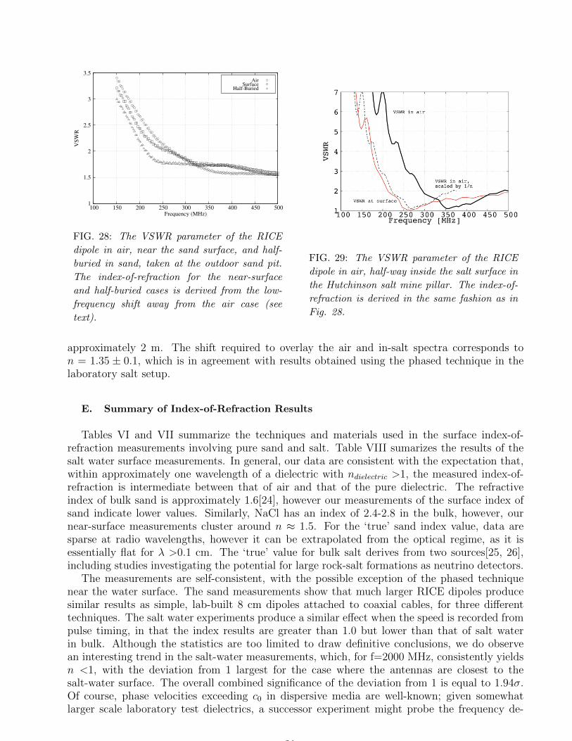
frequency-space of this rapid increase in VSWR decreases by a factor of n. We can therefore usethe evolution of the VSWR with frequency as a measure of the index-of-refraction. The indexwas determined from the relative shifts in the VSWR spectra (shown in Fig. 28) for the casesof near-surface and half-buried antennas. The average measured refractive index for the nearsurface case is n = 1.08± 0.04, and the half-buried measured refractive index is n = 1.17± 0.04.These results are in agreement with the results derived from the wave speed measurements, andare summarized in Tab. VI below.
Additional measurements were taken in a salt mine in Hutchinson, KS, where the smoothand extensive salt deposits provided a suitable dielectric surface. The VSWR was measured ineach case, confirming the expectation that near the surface, the low-frequency cutoff of antennaradiation decreased by a factor of n. One such result is shown in Fig. 29. The RICE dipoleswere used as probes, where the relevant frequency is again ∼150 MHz (the cut-in frequency ofthe dipoles near the surface). The antennas were placed perpendicular to the vertical salt wall;i.e., horizontal with respect to the ground. The height of the antennas above the ground was
20
1
1.5
2
2.5
3
3.5
100 150 200 250 300 350 400 450 500
VS
WR
Frequency (MHz)
AirSurface
Half-Buried
FIG. 28: The VSWR parameter of the RICE
dipole in air, near the sand surface, and half-
buried in sand, taken at the outdoor sand pit.
The index-of-refraction for the near-surface
and half-buried cases is derived from the low-
frequency shift away from the air case (see
text).
FIG. 29: The VSWR parameter of the RICE
dipole in air, half-way inside the salt surface in
the Hutchinson salt mine pillar. The index-of-
refraction is derived in the same fashion as in
Fig. 28.
approximately 2 m. The shift required to overlay the air and in-salt spectra corresponds ton = 1.35 ± 0.1, which is in agreement with results obtained using the phased technique in thelaboratory salt setup.
E. Summary of Index-of-Refraction Results
Tables VI and VII summarize the techniques and materials used in the surface index-of-refraction measurements involving pure sand and salt. Table VIII sumarizes the results of thesalt water surface measurements. In general, our data are consistent with the expectation that,within approximately one wavelength of a dielectric with ndielectric >1, the measured index-of-refraction is intermediate between that of air and that of the pure dielectric. The refractiveindex of bulk sand is approximately 1.6[24], however our measurements of the surface index ofsand indicate lower values. Similarly, NaCl has an index of 2.4-2.8 in the bulk, however, ournear-surface measurements cluster around n ≈ 1.5. For the ‘true’ sand index value, data aresparse at radio wavelengths, however it can be extrapolated from the optical regime, as it isessentially flat for λ >0.1 cm. The ‘true’ value for bulk salt derives from two sources[25, 26],including studies investigating the potential for large rock-salt formations as neutrino detectors.
The measurements are self-consistent, with the possible exception of the phased techniquenear the water surface. The sand measurements show that much larger RICE dipoles producesimilar results as simple, lab-built 8 cm dipoles attached to coaxial cables, for three differenttechniques. The salt water experiments produce a similar effect when the speed is recorded frompulse timing, in that the index results are greater than 1.0 but lower than that of salt waterin bulk. Although the statistics are too limited to draw definitive conclusions, we do observean interesting trend in the salt-water measurements, which, for f=2000 MHz, consistently yieldsn <1, with the deviation from 1 largest for the case where the antennas are closest to thesalt-water surface. The overall combined significance of the deviation from 1 is equal to 1.94σ.Of course, phase velocities exceeding c0 in dispersive media are well-known; given somewhatlarger scale laboratory test dielectrics, a successor experiment might probe the frequency de-
21
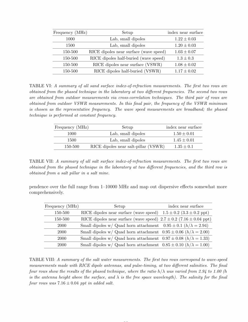
Frequency (MHz) Setup index near surface
1000 Lab, small dipoles 1.22± 0.03
1500 Lab, small dipoles 1.20± 0.03
150-500 RICE dipoles near surface (wave speed) 1.03± 0.07
150-500 RICE dipoles half-buried (wave speed) 1.3± 0.3
150-500 RICE dipoles near surface (VSWR) 1.08± 0.02
150-500 RICE dipoles half-buried (VSWR) 1.17± 0.02
TABLE VI: A summary of all sand surface index-of-refraction measurements. The first two rows are
obtained from the phased technique in the laboratory at two different frequencies. The second two rows
are obtained from outdoor measurements via cross-correlation techniques. The third pair of rows are
obtained from outdoor VSWR measurements. In this final pair, the frequency of the VSWR minimum
is chosen as the representative frequency. The wave speed measurements are broadband; the phased
technique is performed at constant frequency.
Frequency (MHz) Setup index near surface
1000 Lab, small dipoles 1.50± 0.01
1500 Lab, small dipoles 1.45± 0.01
150-500 RICE dipoles near salt-pillar (VSWR) 1.35± 0.1
TABLE VII: A summary of all salt surface index-of-refraction measurements. The first two rows are
obtained from the phased technique in the laboratory at two different frequencies, and the third row is
obtained from a salt pillar in a salt mine.
pendence over the full range from 1–10000 MHz and map out dispersive effects somewhat morecomprehensively.
Frequency (MHz) Setup index near surface
150-500 RICE dipoles near surface (wave speed) 1.5± 0.2 (3.3± 0.2 ppt)
150-500 RICE dipoles near surface (wave speed) 2.7± 0.2 (7.16± 0.04 ppt)
2000 Small dipoles w/ Quad horn attachment 0.95± 0.1 (h/λ = 2.94)
2000 Small dipoles w/ Quad horn attachment 0.95± 0.06 (h/λ = 2.00)
2000 Small dipoles w/ Quad horn attachment 0.97± 0.08 (h/λ = 1.33)
2000 Small dipoles w/ Quad horn attachment 0.85± 0.10 (h/λ = 1.00)
TABLE VIII: A summary of the salt water measurements. The first two rows correspond to wave-speed
measurements made with RICE dipole antennas, and pulse-timing, at two different salinities. The final
four rows show the results of the phased technique, where the ratio h/λ was varied from 2.94 to 1.00 (h
is the antenna height above the surface, and λ is the free space wavelength). The salinity for the final
four rows was 7.16± 0.04 ppt in added salt.
22
IV. SUMMARY AND CONCLUSIONS
Using a wide range of dielectrics, including pure sand, a sand+metal mixture, ice, and wa-ter with varying amounts of saline impurities, and over a range of frequencies spanning 100MHz–4000 MHz, we have searched for unambiguous evidence for surface wave coupling. Eachindividual experiment includes its own particular systematic errors, which we have not fullyexplored, but rather implicitly “average” over the variety of systematics inherent in our mea-surements. We find no such compelling evidence, and conclude that surface radio-frequencywave detection of neutrinos is unlikely to be a promising experimental avenue.
V. ACKNOWLEDGEMENTS
Data collection for this experiment was primarily performed by Kansas high school stu-dents during the summers of 2012, 2013 and 2014; correspondingly, we would like to thankthe Fermi National Laboratory and the Department of Energy for sponsoring the QuarkNetprogram, through which American high-school physics students are connected with Universityresearchers. We also would like to acknowledge Marie Piasecki (NASA) and John Ralston (KU)for their helpful discussions early in this project, and Jeffrey Engelstad for his assistance withthe Great Sand Dunes National Park measurements. Finally, we thank the staff at KU FacilitiesManagement and the Hutchinson Salt Mine for their support and cooperation.
[1] V.S. Berezinsky and G.T. Zatsepin. On the origin of cosmic rays at high energies. Phys. Lett. B,
28:423, 1969.
[2] K. Greisen. End to the cosmic-ray spectrum? Phys. Rev. D, 16:748–750, 1966.
[3] G.T. Zatsepin and V.A. Kuz’min. Upper limit of the spectrum of cosmic rays. JETP Letters,
4:78–80, 1966.
[4] G. Askaryan. Excess negative charge of an electron-photon shower and its coherent radio emission.
Soviet Physics JETP, 14:441–443, 1962.
[5] F. Halzen E. Zas and T. Stanev. Electromagnetic pulses from high energy showers. Phys. Rev. D,
45:362–376, 1992.
[6] J.C. Hanson et al. (The ARIANNA Collaboration). Radar absorption, basal reflection, thickness,
and polarization measurements from the ross ice shelf. Journal of Glaciology, 61, 227, 2015.
[7] D. Saltzberg T. Barrella and S.W. Barwick. Ross ice shelf (antarctica) in situ radio-frequency
attenuation. J. of Glac., 57:61–66, 2011.
[8] J. Zenneck. ber die fortpflanzung ebener elektromagnetischer wellen lngs einer ebenen leiterflche
und ihre beziehung zur drahtlosen telegraphie. Ann. der Physik, 23, 1907.
[9] Klaas Wynne and Dino A. Jaroszynski. Superluminal terahertz pulses. Optics Letters, 24, 1999.
[10] A. Sommerfeld. ber die ausbreitung der wellen in der drahtlosen telegraphie. Ann. der Physik,
28:665–736, 1909.
[11] John P. Ralston. Radio surf in polar ice: A new method of ultrahigh energy neutrino detection.
Phys. Rev. D, 71:011503–1, 2005.
[12] P. Hansen. A study of vhf radio wave propagation over a water surface of variable conductivity.
Radio Science, 12:397–404, 1977.
[13] D.E. Barrick. Theory of hf and vhf propagation across the rough sea, 2, application to hf and vhf
propagation above the sea. Radio Science, 6:517–533, 1971.
[14] J. R. Wait. Electromagnetic surface waves. Advances in Radio Research, 1:157–217, 1964.
23
[15] Kistovich Y.V.R. Baibakov V.I., Datsko V.N. Journal of Technical Physics Letters (in Russian),
6, 7:394–400, 1980.
[16] Kistovich Y.V.R. Baibakov V.I. Journal of Technical Physics (in Russian), 52, 5:846–852, 1982.
[17] Kistovich Y.V.R. Baibakov V.I., Datsko V.N. Physics Achievements (in Russian), 157, 4:722–725,
1989.
[18] A. Ranfagni D. Mugnai and R. Ruggeri. Observation of superluminal behaviors in wave propaga-
tion. Physical Review Letters, 84, 2000.
[19] N. P. Bigelow and C. R. Hagen. Comment on observation of superluminal behaviors in wave
propagation. Physical Review Letters, 87, 2001.
[20] H. Ringermacher and L. Mead. Comment on observation of superluminal behaviors in wave prop-
agation. Physical Review Letters, 87, 2001.
[21] R. Ranfagi et al. Observation of zenneck-type waves in microwave propagation experiments. J.
Appl. Phys., 100(024910):88–102, 2006.
[22] I. Kravchenko et al. Updated results from the rice experiment and future prospects for ultra-high
energy neutrino detection at the south pole. Phys. Rev. Lett. D, 85:062004, 2012.
[23] P. Allison et al. Design and initial performance of the askaryan radio array prototype eev neutrino
detector at the south pole. Astroparticle Physics, 35, 2012.
[24] Christian Matzler. Microwave permittivity of dry sand. IEEE Trans. on Geosci. and Rem. Sens.,
36(1):317–319, 1998.
[25] A. Connolly et al. Measurements of radio propagation in rock salt for the detection of high-energy
neutrinos. Nucl. Inst. and Meth. in Phys. Res. A, 599(2-3):184–191, 2009.
[26] P. Gorham et al. Measurements of the suitability of large rock salt formations for radio detection
of high energy neutrinos. Nucl. Inst. and Meth. in Phys. Res. A, 490:476–491, 2002.
[27] R. Somaraju et al. Frequency, temperature and salinity variation of the permittivity of seawater.
IEEE Transactions on Antennas and Propagation, 54(11):3441–3448, 2006.
24