pdf - grass tutorial - grass gis
TRANSCRIPT

Grass Tutorialby Moritz Lennert
Published $Date: 2005/04/26 15:39:13 $
Geographic Resources Analysis Support System Tutorial
(Please note, the current version only outlines the intended contents, pages may be missing!)
Copyright (c) 2003 GRASS Development Team. Permission is granted to copy, distributeand/or modify this document under the terms of the GNU Free Documentation License,Version 1.2 or any later version published by the Free Software Foundation; with no InvariantSections, no Front-Cover Texts, and no Back-Cover Texts. A copy of the license is included inthe section entitled "GNU Free Documentation License".
Table of ContentsI. Introduction........................................................................................................................1
1. About this tutorial ....................................................................................................12. What is GRASS ? ......................................................................................................33. Credits........................................................................................................................5
II. Basics..................................................................................................................................74. Hardware and software requirements ..................................................................7
Hardware .............................................................................................................7Basic Software .....................................................................................................7Optional software ...............................................................................................7
5. Basic UNIX reference .............................................................................................116. Download and Install ............................................................................................13
Packages of GNU/Linux Distributions.........................................................13Compilation of source code.............................................................................13
III. GRASS in 10 minutes - Quick Intro for Newbies .................................................157. How to Quickstart GRASS....................................................................................15
You have a GRASS database ...........................................................................15You have a georeferenced data file, and know its geographical
coordinates ...............................................................................................16You have a georeferenced raster file, but don’t know its geographical
coordinates ...............................................................................................16You have a non-georeferenced data file ........................................................17Other situations.................................................................................................17
8. The Most Important Commands to Get Started ................................................19IV. GRASS Concepts..........................................................................................................21
9. GRASS structure.....................................................................................................2110. GRASS commands ...............................................................................................2311. Graphical User Interface .....................................................................................2512. The GRASS Region ..............................................................................................27
What is the region.............................................................................................27Why care about the region ..............................................................................27How to work with the region .........................................................................27How to change the default region..................................................................28
V. Start a Project..................................................................................................................3113. Set-up your GRASS database .............................................................................3114. Start running GRASS ...........................................................................................3315. Planning and constructing a GRASS database ................................................35
General definition of a project area when using scanned maps ................35Definition of a project area with predefined geographical resolution ......36Definition of the project area without a previously defined resolution ...37
16. Set-up your location.............................................................................................3917. Manage your data ................................................................................................43
VI. Import Data ...................................................................................................................4518. Supported formats ...............................................................................................4519. Raster Import ........................................................................................................4720. Vector Import ........................................................................................................4921. Sites (point data) import......................................................................................51
VII. Display and Query Maps ..........................................................................................5322. Managing GRASS Monitors ...............................................................................53
Frames in monitors...........................................................................................5323. Displaying Maps ..................................................................................................55
Colors .................................................................................................................55Scripting the display of maps (and frames)..................................................55
24. Zooming and Panning.........................................................................................5725. Adding Legends and Scales................................................................................5926. Visualize in 3D with nviz ....................................................................................61
iii
VIII. Digitize........................................................................................................................6327. Digitizing Vector Maps........................................................................................63
Rules for Digitizing in Topological GIS.........................................................63Digitizing Maps ................................................................................................63Digitizing Areas ................................................................................................64Digitizing of Elevation Isolines ......................................................................66
28. Processing Scanned Maps ...................................................................................69Geocoding of scanned maps ...........................................................................69Gap free geocoding of multiple, adjacent, scanned maps ..........................72
IX. Manage Attributes and Classes .................................................................................7529. Raster Categories and Attributes .......................................................................75
Viewing category values..................................................................................75Changing category values ...............................................................................75
30. Vector Categories and Attributes.......................................................................77Viewing category values..................................................................................77Changing category values ...............................................................................77
31. Site Attributes .......................................................................................................7932. Data Management with PostgreSQL.................................................................81
X. Analyze Maps .................................................................................................................8333. Statistics and Reports...........................................................................................83
Modules for raster maps..................................................................................83Modules for vector maps.................................................................................84Modules for site maps......................................................................................84
34. Overlay and Patch Maps.....................................................................................8735. Create Buffers........................................................................................................8936. Raster map algrebra with r.mapcalc ..................................................................91
XI. Transform .......................................................................................................................9337. Coordinate Systems .............................................................................................93
Introduction to projections and coordinate systems ...................................93Projections in GRASS .......................................................................................93
38. Project data............................................................................................................9539. Raster to Vector.....................................................................................................97
Lines....................................................................................................................97Areas...................................................................................................................97Contours.............................................................................................................97
40. Raster to Sites........................................................................................................9941. Vector to raster ....................................................................................................10142. Vector to Sites......................................................................................................10343. Sites to raster .......................................................................................................10544. Sites to vector ......................................................................................................107
XII. Process Images...........................................................................................................10945. Preprocessing Images ........................................................................................109
Import and export of imagery data..............................................................109Image groups...................................................................................................109Geocoding of images......................................................................................109Colors ...............................................................................................................110Displaying images ..........................................................................................110Radiometric preprocessing............................................................................110
46. Analyzing Images ..............................................................................................113Introduction.....................................................................................................113Image ratios .....................................................................................................113Factor analysis.................................................................................................113Fourier transformation...................................................................................113Image filtering .................................................................................................113
47. Classifying Images .............................................................................................115Introduction.....................................................................................................115Unsupervised classification...........................................................................115Supervised classification................................................................................115
iv
Partially supervised classification................................................................116XIII. Cartography ..............................................................................................................117
48. Introduction ........................................................................................................11749. Map export to raster image files ......................................................................119
PNG driver ......................................................................................................119CELL driver .....................................................................................................119Scripting the creation of maps ......................................................................119Creating a PNG map from the Display Manager ......................................120
50. Postscript Maps/Exports ..................................................................................123Interactive usage .............................................................................................123Scripted usage .................................................................................................123Editing the resulting postscript file with pstoedit .....................................124
51. HTML Maps/Exports........................................................................................12552. Using external programs for map layout .......................................................127
XIV. Programming............................................................................................................12953. Scripting GRASS.................................................................................................129
Scripts ...............................................................................................................129Batch usage of GRASS ...................................................................................129
54. C-Programming..................................................................................................131XV. Special Topics ............................................................................................................135
55. Digital Terrain Models.......................................................................................13556. Topographical analysis ......................................................................................13757. Cost Surfaces.......................................................................................................13958. Creating Animations..........................................................................................141
XVI. Bibliography.............................................................................................................14359. Bibliography........................................................................................................143
A. GNU Free Documentation License ..........................................................................145PREAMBLE...............................................................................................................145APPLICABILITY AND DEFINITIONS.................................................................145VERBATIM COPYING ............................................................................................146COPYING IN QUANTITY......................................................................................146MODIFICATIONS....................................................................................................147COMBINING DOCUMENTS.................................................................................148COLLECTIONS OF DOCUMENTS.......................................................................149AGGREGATION WITH INDEPENDENT WORKS............................................149TRANSLATION........................................................................................................149TERMINATION........................................................................................................149FUTURE REVISIONS OF THIS LICENSE............................................................150ADDENDUM: How to use this License for your documents ...........................150
v

vi

Chapter 1. About this tutorial
This tutorial (or maybe it should rather be calles manual ?) should help you getstarted with GRASS1. It gives basic explanations of how GRASS functions and linksto the relevant man pages and other documentation.
Several chapters in this tutorial contain content taken from the english translationof Markus Neteler’s GRASS Handbook2, (c) 1996-2001, Markus Neteler. I have notincluded explicit references each time I’ve used excerpts, but it is the most importantsource of text in these pages.
Notes1. http://grass.itc.it/
2. http://grass.itc.it/gdp/handbuch/index.html
1

Chapter 1. About this tutorial
2
Chapter 2. What is GRASS ?
GRASS - Geographic Resources Analysis Support System is a general GIS supportingprocessing, analysis and display of raster, vector, site and imagery data, geospatialsimulations and visualization.
For a general introduction, see the GRASS First Time User Page1.
Overview of GRASS versions currently available:
• CVS GRASS6 - continuously updated developers version - see GRASS CVS page2
• GRASS6.1 - under development, see GRASS6 page3
• GRASS6.0 - current stable release, see GRASS6 page4
• GRASS4.3- last non-floating point release - see GRASS4.3 release page5
• GRASS4.1- latest official CERL release 1991 - see GRASS4.1 release page6
GRASS is an Open source sofware released under the GNU General Public Licence7
- it is therefore free with protection of the authors’ rights. With its 1.5 million lines ofC code, it is one of the largest Open source projects.
Notes1. http://grass.itc.it/intro/firsttime.php
2. http://grass.itc.it/devel/cvs.php
3. http://grass.itc.it/grass60/index.php
4. http://grass.itc.it/grass60/index.php
5. http://grass.itc.it/announces/4.3release.info.html
6. http://grass.itc.it/announces/4.1release.info.html
7. http://www.gnu.org
3

Chapter 2. What is GRASS ?
4
Chapter 3. Credits
• History of GRASS1
• Credits2
• Current development team3
Notes1. http://grass.itc.it/devel/grasshist.html
2. http://grass.itc.it/devel/grasscredits.html
3. http://freegis.org/cgi-bin/viewcvs.cgi/~checkout~/grass/AUTHORS
5

Chapter 3. Credits
6
Chapter 4. Hardware and software requirements
Hardware
A workstation running some flavor of UNIX like Solaris, IRIX, GNU/Linux, BSD,Mac OS X. GRASS also runs on on Win32 within the Cygwin environment1. As aminimum, you should have at least 500 Mb for data and 32 Mb RAM. However thiswill allow you only a very limited usage of GRASS (although see here2 for GRASSon handhelds). For a serious usage of GRASS you will need 128MB at the very least.Obviously, a good video card is a must for cartography, ideally with 3D support.
Basic Software
• C-compiler (cc, gcc, egcs, ...)
gcc: http://www.gnu.org/software/gcc/gcc.html
• GNU make is recommended
http://www.gnu.org/software/make/make.html
• zlib compression library (already installed on modern systems)
It is used to internally compress GRASS raster files: libz:http://www.gzip.org/zlib/
• lexical analyzer generator (flex),
(lex is no longer supported, please use flex instead) - flex:http://www.gnu.org/software/flex/flex.html
• parser generator (yacc, bison)
bison: http://www.gnu.org/software/bison/bison.html
• libncurses4.x/5.x (already installed on modern systems)
http://www.gnu.org/software/ncurses/ncurses.html
ftp://ftp.gnu.org/pub/gnu/ncurses/
• dgm/gdbm (dbm.h): GNU dbm is a set of database routines that use extendiblehashing and works similar to the standard UNIX dbm routines. Currently not re-quired.
http://www.gnu.org/software/gdbm/gdbm.html
• X11 window system for graphical output, development libraries (X developmentlibraries, in some linux distributions they are separate packages)
http://www.xfree.org
(winGRASS: As alternative a generic MS-Windows driver is under constructionwhich does not require X11)
7
Chapter 4. Hardware and software requirements
Optional software
• Tcl/Tk 8.x libraries (they include ’wish’) to use TclTkGRASS Interface and to com-pile src.contrib/GMSL/NVIZ2.2/
http://tcl.sourceforge.net/
• Mesa-3.x (openGL clone) required for NVIZ2.2 (if your OS / graphic card librariesdon’t come with own OpenGL libraries)
http://mesa3d.sourceforge.net/
• FFTW (library for computing the Discrete Fourier Transform) required for i.fft andi.ifft modules
http://www.fftw.org
• LAPACK / BLAS (libraries for numerical computing) required for GMATH library(GRASS numerical lib)
http://www.netlib.org/lapack/ (usually present in Linux distros)
Note: the support is intended for future module implementations
• libpng (for r.in.png, r.out.png), usually already installed.>
http://www.libpng.org/pub/png/libpng.html
• libjpeg (for r.in.tiff, r.out.tiff), usually already installed.
http://www.ijg.org17
ftp://ftp.uu.net/graphics/jpeg/
• libtiff (for r.in.tiff, r.out.tiff), usually already installed.
http://www.libtiff.org
• libgd (for PNG driver), preferably GD 2.x.
http://www.boutell.com/gd/
• netpbm-tools/libraries (for r.in.png/r.out.png), usually already installed.
(please look at any decent software mirror near you!)
http://netpbm.sourceforge.net/
http://www.sourceforge.net/projects/netpbm/
• PostgreSQL libraries (for the PostgreSQL database interface)
http://www.postgresql.org
• Unix ODBC (for the ODBC database interface)
http://www.unixodbc.org
8
Chapter 4. Hardware and software requirements
• Only required for "xanim" and "ogl3d": the Motif or Lesstif libraries
http://www.lesstif.org
• r.in.gdal requires GDAL - Geospatial Data Abstraction Library
http://www.remotesensing.org/gdal/
• R language (for the R language interface)
http://cran.r-project.org
• FreeType2 (for d.text.freetype)
http://www.freetype.org/
Notes1. http://www.cygwin.com
2. http://grass.itc.it/platforms/grasshandheld.html
3. http://www.gnu.org/software/gcc/gcc.html
4. http://www.gnu.org/software/make/make.html
5. http://www.gzip.org/zlib/
6. http://www.gnu.org/software/flex/flex.html
7. http://www.gnu.org/software/bison/bison.html
8. http://www.gnu.org/software/ncurses/ncurses.html
9. ftp://ftp.gnu.org/pub/gnu/ncurses/
10. http://www.gnu.org/software/gdbm/gdbm.html
11. http://www.xfree.org
12. http://tcl.sourceforge.net/
13. http://mesa3d.sourceforge.net/
14. http://www.fftw.org
15. http://www.netlib.org/lapack/
16. http://www.libpng.org/pub/png/libpng.html
17. http://www.ijg.org/
18. ftp://ftp.uu.net/graphics/jpeg/
19. http://www.libtiff.org
20. http://www.boutell.com/gd/
21. http://netpbm.sourceforge.net/
22. http://www.sourceforge.net/projects/netpbm/
23. http://www.postgresql.org
24. http://www.unixodbc.org
25. http://www.lesstif.org
26. http://www.remotesensing.org/gdal/
27. http://cran.r-project.org
9

Chapter 4. Hardware and software requirements
28. http://www.freetype.org/
10
Chapter 5. Basic UNIX reference
Since GRASS runs in a UNIX / GNU / Linux environnement, general knowledge ofbasic UNIX commands is recommended. Here are a few links to introductions andtutorials:
• Linux Cookbook1
• The Linux Users’ Guide2
• Unix commands reference card3
• Introduction to Linux4
Notes1. http://www.dsl.org/cookbook/
2. http://www.ibiblio.org/pub/Linux/docs/linux-doc-project/users-guide/
3. http://www.indiana.edu/~uitspubs/b017/
4. http://www.tldp.org/LDP/intro-linux/html/index.html
11

Chapter 5. Basic UNIX reference
12
Chapter 6. Download and Install
Get GRASS from the Download Page1 on the server in Italy or from one of the MirrorSites2.
For a very thourough introduction about GRASS (and Linux) installation, please seeA.P. Pradeepkumar’s Absolute beginner’s Guide to GRASS Installation (PDF, 277K)3.
Packages of GNU/Linux Distributions
Binary packages have been created for major GNU/Linux distributions . The can bedownloaded at GRASS downlaod page4
Mandrake
In Mandrake 9.0 and later, GRASS is included in the contribs. To install use theSoftware Installer in the Mandrake Control Center, or run ’urpmi grass’ as root.
Debian
GRASS is included in Debian testing and unstable. You may also check DebianGIS repository5
SuSE
SuSE rpms are avalaible on GRASS download page.
Live CD
You can buy the FreeGIS CD6 which contains GRASS and much more.
Compilation of source code
You can also download and compile the entire source code yourself. This allows youto have access to the code and modify it if you would like to.
The source is more or less platform independent and is available athttp://grass.itc.it/download/index.php. For GRASS 6.0 get the grass-6.0.0.tar.gzfile, put it into the directory of your choice and decompress it with:
gunzip grass6.0.0.tar.gz; tar -xvf grass6.0.0.tar
or
tar -xvzf grass6.0.0.tar.gz
Then follow the installation instructions8 also included in the source code archive youdownloaded. Also, don’t forget to read the list of required software 9 or Chapter 4 inthis tutorial.
Notes1. http://grass.itc.it/download/index.php
2. http://grass.itc.it/mirrors.php
3. http://grass.itc.it//gdp/tutorial/abs_beginners.pdf
4. http://grass.itc.it/download/index.php
5. http://pkg-grass.alioth.debian.org/cgi-bin/wiki.pl
6. http://www.freegis.org/cd-contents.en.html
7. http://grass.itc.it/download/index.php
8. http://grass.itc.it/grass60/source/INSTALL
13

Chapter 6. Download and Install
9. http://grass.itc.it/grass60/source/REQUIREMENTS.html
14
Chapter 7. How to Quickstart GRASS
This chapter aims at giving a newcomer in GRASS a very hands-on introduction inorder to give him the opportunity to very quickly take first tentative steps in GRASS.This does not replace a throrough study of the rest of the documentation, but shouldhelp relieve the frustrations that many newbies feel at the first contact with GRASS.It will cover GRASS 6.0, so if you have an earlier version, consider upgrading.
This introduction assumes that you have already successfully installed GRASS, butthat you have not yet launched a GRASS session successfully. If you haven’t installedGRASS, yet, please have a look at Chapter 6. For newbies, the binary installation isrecommended. If you are unfamiliar with the UNIX or GNU/Linux environment,please go to Chapter 5 first and follow some of the links there.
Before going any further, you will have to create the GRASS database:
1. Find a place on your disk where you have write access and that has enoughdiskspace to hold your decompressed data.
2. Create a subdirectory that will hold the general GRASS database (e.g. "mkdir/data/GRASSDATA" or "mkdir /home/yourlogin/GRASSDATA").
Now you can go on. The following subsections will cover different potential "scenar-ios", each representative of the situations in which a new user might turn to GRASS:
• If you have a GRASS database, either because someone gave you one, or becauseyou downloaded sample data such as the Spearfish sample dataset1 (see here2 forother data sets), then see the Section called You have a GRASS database.
• If you have a georeferenced data file (raster, vector or sites) and know its geograph-ical projection, its extension, and its resolution (for raster), then see the Sectioncalled You have a georeferenced data file, and know its geographical coordinates.
• If you have a georeferenced raster file, but do not know its projection, extension,or resolution, then see the Section called You have a georeferenced raster file, but don’tknow its geographical coordinates.
• If you have a non-georeferenced data file (example scanned map), then see theSection called You have a non-georeferenced data file.
• Other, see the Section called Other situations
You have a GRASS database
You have a tar ball (*.tgz, *.tar.gz, *.tar) with an already prepared GRASS location.Here are the steps to follow:
1. Enter the GRASS database directory you created above and untar your data filein there (e.g. "tar xvzf /path/to/where/you/downloaded/yourdatafile.tgz").This should create a directory containing the sample location (e.g. spearfish60),with several subdirectories, each of these representing a mapset. There shouldbe at least one, called "PERMANENT" (note the names of the others). Don’ttouch anything in this directory.
2. Go back to your home directory ("cd") and start GRASS ("grass").
3. First specify in the Database field the absolute path to the directory you cre-ated above (e.g. "/data/GRASSDATA"). You can now choose the location. Ifyou download sampledata, it will be spearfish60. Now, you should see at leastPERMANENT in the mapsets list. You can create a new mapset by enter itsname in the left field and click on "Create..." button. Select one them on themapsets list. Click on "Enter GRASS" button.
4. The GIS Manager should start automatically.
15
Chapter 7. How to Quickstart GRASS
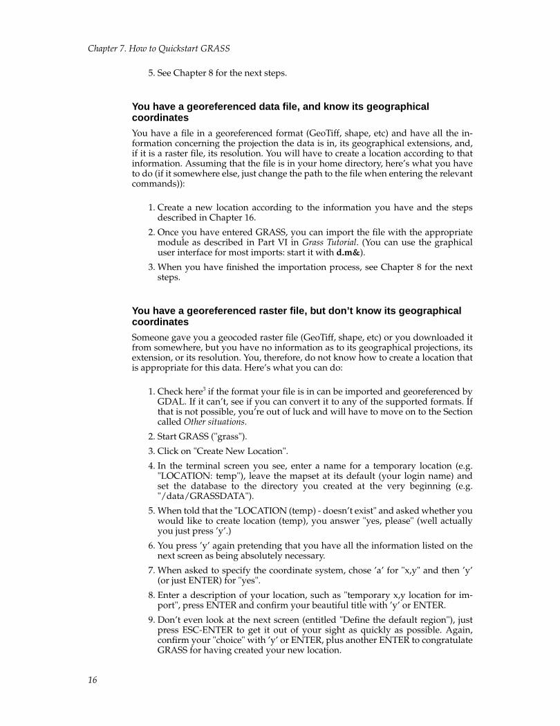
5. See Chapter 8 for the next steps.
You have a georeferenced data file, and know its geographicalcoordinates
You have a file in a georeferenced format (GeoTiff, shape, etc) and have all the in-formation concerning the projection the data is in, its geographical extensions, and,if it is a raster file, its resolution. You will have to create a location according to thatinformation. Assuming that the file is in your home directory, here’s what you haveto do (if it somewhere else, just change the path to the file when entering the relevantcommands)):
1. Create a new location according to the information you have and the stepsdescribed in Chapter 16.
2. Once you have entered GRASS, you can import the file with the appropriatemodule as described in Part VI in Grass Tutorial. (You can use the graphicaluser interface for most imports: start it with d.m&).
3. When you have finished the importation process, see Chapter 8 for the nextsteps.
You have a georeferenced raster file, but don’t know its geographicalcoordinates
Someone gave you a geocoded raster file (GeoTiff, shape, etc) or you downloaded itfrom somewhere, but you have no information as to its geographical projections, itsextension, or its resolution. You, therefore, do not know how to create a location thatis appropriate for this data. Here’s what you can do:
1. Check here3 if the format your file is in can be imported and georeferenced byGDAL. If it can’t, see if you can convert it to any of the supported formats. Ifthat is not possible, you’re out of luck and will have to move on to the Sectioncalled Other situations.
2. Start GRASS ("grass").
3. Click on "Create New Location".
4. In the terminal screen you see, enter a name for a temporary location (e.g."LOCATION: temp"), leave the mapset at its default (your login name) andset the database to the directory you created at the very beginning (e.g."/data/GRASSDATA").
5. When told that the "LOCATION (temp) - doesn’t exist" and asked whether youwould like to create location (temp), you answer "yes, please" (well actuallyyou just press ’y’.)
6. You press ’y’ again pretending that you have all the information listed on thenext screen as being absolutely necessary.
7. When asked to specify the coordinate system, chose ’a’ for "x,y" and then ’y’(or just ENTER) for "yes".
8. Enter a description of your location, such as "temporary x,y location for im-port", press ENTER and confirm your beautiful title with ’y’ or ENTER.
9. Don’t even look at the next screen (entitled "Define the default region"), justpress ESC-ENTER to get it out of your sight as quickly as possible. Again,confirm your "choice" with ’y’ or ENTER, plus another ENTER to congratulateGRASS for having created your new location.
16
Chapter 7. How to Quickstart GRASS
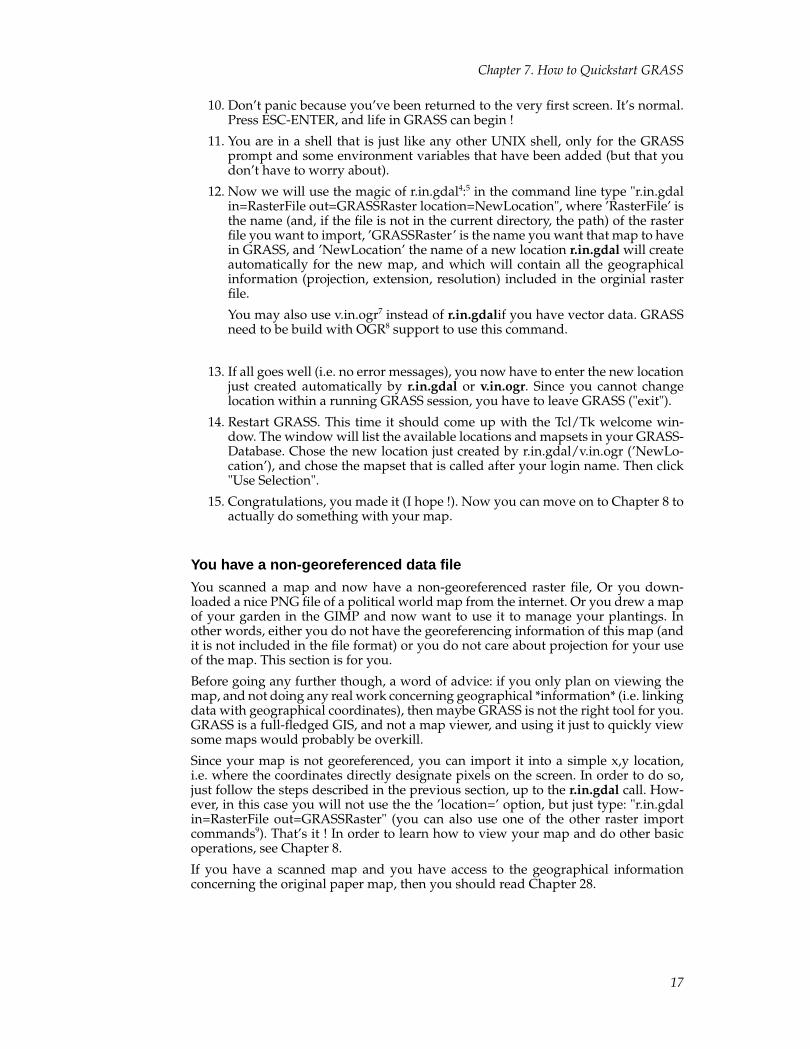
10. Don’t panic because you’ve been returned to the very first screen. It’s normal.Press ESC-ENTER, and life in GRASS can begin !
11. You are in a shell that is just like any other UNIX shell, only for the GRASSprompt and some environment variables that have been added (but that youdon’t have to worry about).
12. Now we will use the magic of r.in.gdal4:5 in the command line type "r.in.gdalin=RasterFile out=GRASSRaster location=NewLocation", where ’RasterFile’ isthe name (and, if the file is not in the current directory, the path) of the rasterfile you want to import, ’GRASSRaster’ is the name you want that map to havein GRASS, and ’NewLocation’ the name of a new location r.in.gdal will createautomatically for the new map, and which will contain all the geographicalinformation (projection, extension, resolution) included in the orginial rasterfile.
You may also use v.in.ogr7 instead of r.in.gdalif you have vector data. GRASSneed to be build with OGR8 support to use this command.
13. If all goes well (i.e. no error messages), you now have to enter the new locationjust created automatically by r.in.gdal or v.in.ogr. Since you cannot changelocation within a running GRASS session, you have to leave GRASS ("exit").
14. Restart GRASS. This time it should come up with the Tcl/Tk welcome win-dow. The window will list the available locations and mapsets in your GRASS-Database. Chose the new location just created by r.in.gdal/v.in.ogr (’NewLo-cation’), and chose the mapset that is called after your login name. Then click"Use Selection".
15. Congratulations, you made it (I hope !). Now you can move on to Chapter 8 toactually do something with your map.
You have a non-georeferenced data file
You scanned a map and now have a non-georeferenced raster file, Or you down-loaded a nice PNG file of a political world map from the internet. Or you drew a mapof your garden in the GIMP and now want to use it to manage your plantings. Inother words, either you do not have the georeferencing information of this map (andit is not included in the file format) or you do not care about projection for your useof the map. This section is for you.
Before going any further though, a word of advice: if you only plan on viewing themap, and not doing any real work concerning geographical *information* (i.e. linkingdata with geographical coordinates), then maybe GRASS is not the right tool for you.GRASS is a full-fledged GIS, and not a map viewer, and using it just to quickly viewsome maps would probably be overkill.
Since your map is not georeferenced, you can import it into a simple x,y location,i.e. where the coordinates directly designate pixels on the screen. In order to do so,just follow the steps described in the previous section, up to the r.in.gdal call. How-ever, in this case you will not use the the ’location=’ option, but just type: "r.in.gdalin=RasterFile out=GRASSRaster" (you can also use one of the other raster importcommands9). That’s it ! In order to learn how to view your map and do other basicoperations, see Chapter 8.
If you have a scanned map and you have access to the geographical informationconcerning the original paper map, then you should read Chapter 28.
17
Chapter 7. How to Quickstart GRASS
Other situations
So, you have a file, without much information about it, but you think (or know) itshould be georeferenced. For example, someone sent you an ESRI shape file contain-ing a map you would like to work on. Or you received a raster in a binary format thatis not supported by the GDAL library. Here are some tips on what you might wantto do, depending on the usage you will make of the file:
• Ask the person who sent you the maps to give you more information.
• Think about the data. What is it displaying (political boundaries of countries, asatellite image of jungle areas, etc), what is its rough geographical extension (theWorld or your hometown) ? Where does the data come from (NASA, a personaldigitization, etc). All these factors might give you a lead about the structure of thedata.
• Try to load your data into different locations (see Chapter 16 for the creation of a lo-cation) using widely used projection systems for the area your data is supposed tocover. For example, UTM is widely used in North America, while Gauss-Krueger isoften used in Europe. A lot of the basic shapefiles given out by ESRI are in latitude-longitude "projection". You might want to try the latter first and see how the datalooks. Is it distorted ? Are vector areas not closed ?
• You can also start by creating a simple "x,y" location (see the Section called Youhave a georeferenced raster file, but don’t know its geographical coordinates on how tocreate such a location). Import your data with the appropriate module (see Part VIin Grass Tutorial and then explore it with the commands explained in Chapter 8.
• Good luck !
Notes1. http://grass.itc.it/sampledata/spearfish_grass60data.tar.gz
2. http://grass.itc.it/download/data.php
3. http://www.remotesensing.org/gdal/formats_list.html
4. http://grass.itc.it/grass60/manuals/html60_user/r.in.gdal.html
5. If you compiled GRASS yourself, be sure to also have installed the
6. http://www.remotesensing.org/gdal/, otherwise r.in.gdal will not work. This is also true for v.in.ogr that require OGRlibraries.
6. http://www.remotesensing.org/gdal/
7. http://grass.itc.it/grass60/manuals/html60_user/v.in.ogr.html
8. http://www.gdal.org/ogr/
9. http://grass.itc.it/grass60/manuals/html60_user/raster.html
18
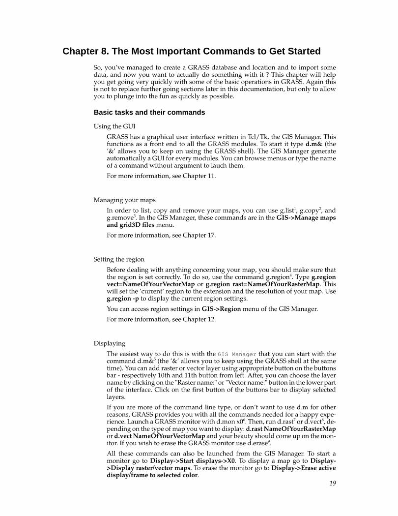
Chapter 8. The Most Important Commands to Get Started
So, you’ve managed to create a GRASS database and location and to import somedata, and now you want to actually do something with it ? This chapter will helpyou get going very quickly with some of the basic operations in GRASS. Again thisis not to replace further going sections later in this documentation, but only to allowyou to plunge into the fun as quickly as possible.
Basic tasks and their commands
Using the GUI
GRASS has a graphical user interface written in Tcl/Tk, the GIS Manager. Thisfunctions as a front end to all the GRASS modules. To start it type d.m& (the’&’ allows you to keep on using the GRASS shell). The GIS Manager generateautomatically a GUI for every modules. You can browse menus or type the nameof a command without argument to lauch them.
For more information, see Chapter 11.
Managing your maps
In order to list, copy and remove your maps, you can use g.list1, g.copy2, andg.remove3. In the GIS Manager, these commands are in the GIS->Manage mapsand grid3D files menu.
For more information, see Chapter 17.
Setting the region
Before dealing with anything concerning your map, you should make sure thatthe region is set correctly. To do so, use the command g.region4. Type g.regionvect=NameOfYourVectorMap or g.region rast=NameOfYourRasterMap. Thiswill set the ’current’ region to the extension and the resolution of your map. Useg.region -p to display the current region settings.
You can access region settings in GIS->Region menu of the GIS Manager.
For more information, see Chapter 12.
Displaying
The easiest way to do this is with the GIS Manager that you can start with thecommand d.m&5 (the ’&’ allows you to keep using the GRASS shell at the sametime). You can add raster or vector layer using appropriate button on the buttonsbar - respectively 10th and 11th button from left. After, you can choose the layername by clicking on the "Raster name:" or "Vector name:" button in the lower partof the interface. Click on the first button of the buttons bar to display selectedlayers.
If you are more of the command line type, or don’t want to use d.m for otherreasons, GRASS provides you with all the commands needed for a happy expe-rience. Launch a GRASS monitor with d.mon x06. Then, run d.rast7 or d.vect8, de-pending on the type of map you want to display: d.rast NameOfYourRasterMapor d.vect NameOfYourVectorMap and your beauty should come up on the mon-itor. If you wish to erase the GRASS monitor use d.erase9.
All these commands can also be launched from the GIS Manager. To start amonitor go to Display->Start displays->X0. To display a map go to Display->Display raster/vector maps. To erase the monitor go to Display->Erase activedisplay/frame to selected color.
19
Chapter 8. The Most Important Commands to Get Started
If you imported a raster file and GRASS created three files namedNameOfYourRaster.1 , NameOfYourRaster.2 , and NameOfYourRaster.3 , theseprobably represent the three bands of an RGB image. In that case, change thecolor map of these three files to greyscale (thus making the "intensities" ofgrey represent the "intensities" of the respective colors), using r.colors10. Foreach of the three maps type r.colors map=NameOfYourRaster col=grey. Thenyou can use d.rgb11 to display the image: d.rgb r=NameOfYourRasterMap.1g=NameOfYourRasterMap.2 b=NameOfYourRasterMap.3. In the GISManager go to Raster->Manage map colors->Set colors to predefined colortables and chose ’grey’ in the list "Type of color table". Then display withDisplay->Display raster maps->Display RGB overlays.
For more information, see Chapter 23.
Zooming and panning
Use d.zoom12 for zooming and panning. (Beware: this resets your region settings!)
Getting help
You can get help with the g.manual13 command.
Exiting
If you wish to exit GRASS, close the open monitors either by clicking on the closebutton or by using d.mon stop=x014, replacing ’x0’ with the name of whatevermonitor you opened. In the GIS Manager go to Display->Stop displays. Thenyou can simply type exit in the command line and GRASS will close down.
So much for some very basic GRASS usage. For the rest, keep on reading this tutorial,have a look at the rest of the GRASS Documentation Project15 and study the GRASSmanual pages16.
Notes1. http://grass.itc.it/grass60/manuals/html60_user/g.list.html
2. http://grass.itc.it/grass60/manuals/html60_user/g.copy.html
3. http://grass.itc.it/grass60/manuals/html60_user/g.remove.html
4. http://grass.itc.it/grass60/manuals/html60_user/g.region.html
5. http://grass.itc.it/grass60/manuals/html60_user/d.m.html
6. http://grass.itc.it/grass60/manuals/html60_user/d.mon.html
7. http://grass.itc.it/grass60/manuals/html60_user/d.rast.html
8. http://grass.itc.it/grass60/manuals/html60_user/d.vect.html
9. http://grass.itc.it/grass60/manuals/html60_user/d.erase.html
10. http://grass.itc.it/grass60/manuals/html60_user/r.colors.html
11. http://grass.itc.it/grass60/manuals/html60_user/d.rgb.html
12. http://grass.itc.it/grass60/manuals/html60_user/d.zoom.html
13. http://grass.itc.it/grass60/manuals/html60_user/g.manual.html
14. http://grass.itc.it/grass60/manuals/html60_user/d.mon.html
15. http://grass.itc.it/gdp/
16. http://grass.itc.it/grass60/manuals/html60_user/
20
Chapter 9. GRASS structure
Generally speaking, GRASS is a normal user program like many others. It comes witha graphical user interface (GUI) that allows GRASS usage through the mouse. Parallelto that, GIS commands can be entered in the GRASS terminal window. Nevertheless,the program structure is somewhat different to normal user programs: after the start-up of GRASS the GRASS commands (typically called GRASS modules) are at thesame level as the other UNIX commands, meaning that all UNIX commands are alsoavailable in the terminal window where GRASS has been started. This concept allowsthe use of the entire might of UNIX and the programming of powerful procedureswhile working with GRASS. Newcomers to GRASS might have to get used to thisstructure, but they will quickly realize its advantages.
In GRASS GIS data are stored in a directory structure. Before beginning to work withGRASS, the user has to create a "GRASS data subdirectory" (called GRASS database)and specify it later within GRASS. In this directory, GRASS organizes its data au-tomatically through subdirectories. A new subdirectory tree is created for each newproject (called "location") within the database. The organisation of the data should beleft to GRASS. All file operation such as renaming or copying maps involve severalinternal files and should thus always be done only with GRASS commands. Man-ual interventions are acceptable just in exceptional situations. The GRASS graph-ical output, in other words the map display window, is no "normal" window butdisplays geographical data with coordinates. This graphical output window (calledGRASS monitor) can be managed with the GRASS d.mon command. AdditonallyTclTkGRASS allows the configuration and management of these windows.
A few more words about GRASS terminology: as mentioned, a project area is calledlocation in GRASS. It is defined by its geographical boundaries with informationabout coordinates and the map projection. Within this location, area subsections,called mapsets, can be created. Often only one mapset as large as the location isused. Multiple mapsets may be interesting for working groups. Here the "PERMA-NENT" mapset (reserved name) contains maps common for the group, while eachteam member works in his/her own mapset. The database is simply called databasein GRASS.
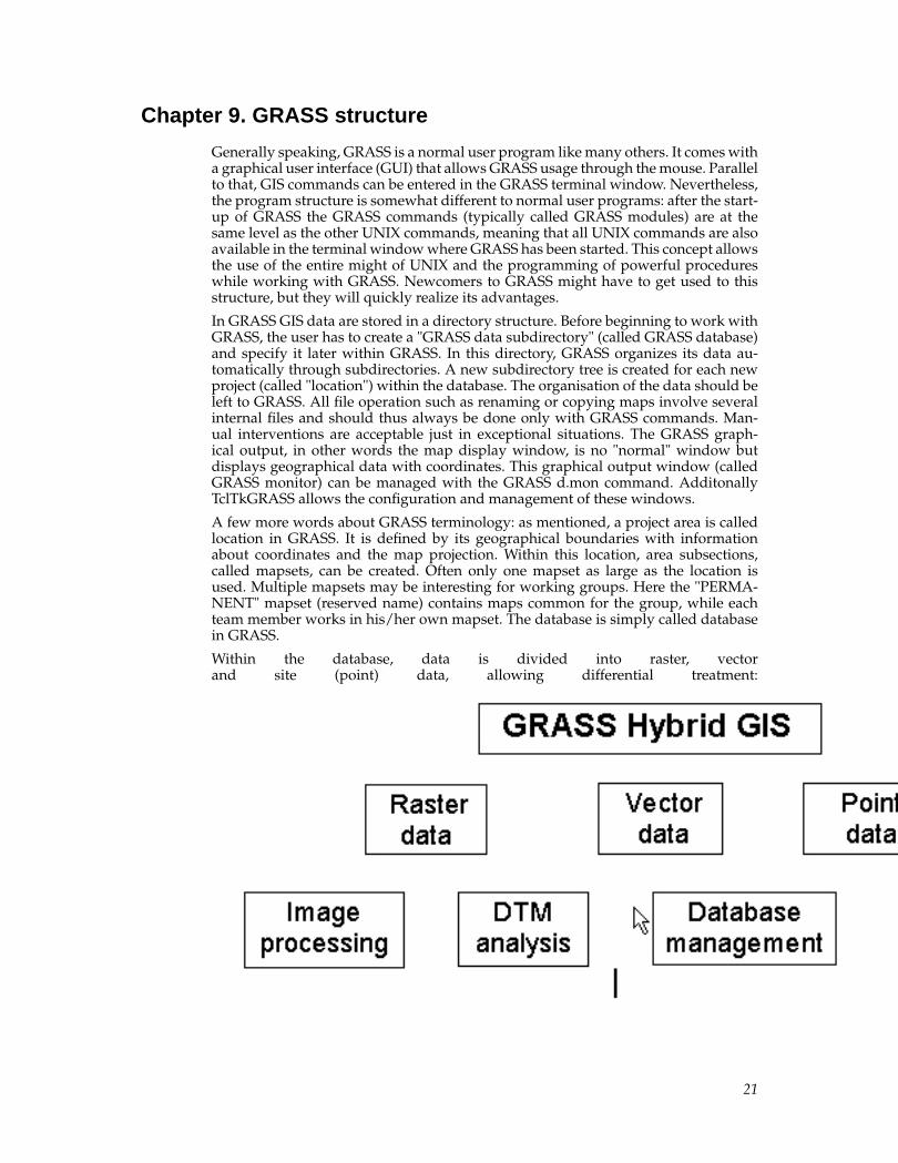
Within the database, data is divided into raster, vectorand site (point) data, allowing differential treatment:
21

Chapter 9. GRASS structure
22
Chapter 10. GRASS commands
The command name indicates its use: first letter indicates data format or generalfunctionality followed by a dot and a short word indicating the task that the com-mand performs:
• d.* - display commands for graphical screen output: d.rast, d.vect, d.sites, d.mon
• g.* - general file management commands: g.list, g.copy
• i.* - image processing commands
• r.* - raster processing commands: r.slope.aspect, r.mapcalc
• v.* - vector processing commands: v.digit, v.to.rast
• s.* - site processing commands (point data): s.univar, s.surf.rst
• m.* - miscellaneous commands: m.in.e00
• p.* / ps.* - map creation (’print’) commands
• ... - unix scripts (some ending in .sh, some imitating GRASS module names)
Almost all modules can be used either directly on the command line (module calland parameters together on one line) or interactively, i.e. you can call each modulewithout parameters, then you will be prompted for required information like mapnames etc.
You can read the manual pages of the commands of GRASS 5.0 online1 or with theg.manual2 command in a running GRASS session (Help->Manual pages in TclTk-GRASS). There is also an (incomplete) one-line reference3 containing a short explana-tion of many commands.
Notes1. http://grass.itc.it/gdp/html_grass5/index.html
2. http://grass.itc.it/gdp/html_grass5/html/g.manual.html
3. http://grass.itc.it/gdp/html_grass5/grass_commandlist.html
23

Chapter 10. GRASS commands
24
Chapter 11. Graphical User Interface
The "TclTkGRASS" GUI which allows mouse usage is simply an extension with-out own GIS functionality. TclTkGRASS offers graphical access to important GRASSmodules and makes working with GRASS easier. However, don’t forget that it is in-complete and that there are many more modules available than are present in theTclTkGrass menus. Also beware that some modules that are present lack some oftheir command line options in their tcltkgrass window.
If TclTkGRASS was not started automatically during GRASS startup, you can do soat the GRASS prompt with the command tcltkgrass&.
25

Chapter 11. Graphical User Interface
26
Chapter 12. The GRASS Region
What is the region
The "region" is a cornerstone concept in GRASS. If you want to be able to use GRASSto its full potential, you have to understand it. In fact, it is so important that youshould know about it even if you only plan some light usage of GRASS. This chapteris an attempt at explaining as clearly as possible what the region is and what itseffects are. It will also, hopefully, help you understand the usefulness of the region inGRASS.
The region defines the geographic area in which GRASS should work. It is character-ized by several parameters:
• geographical projection (e.g. UTM, latitude-longitude, Gauss-Krueger, etc)
• geographical extension, i.e. the North/South/East/West limits of the area covered
• number of columns and number of rows for the data
• resolution, i.e. the extension divided by the number of rows (N-S resolution), re-spectively columns (E-W resolution).
The default values of these parameters for a given location are stored in theDEFAULT_WINDfile in the PERMANENTmapset of that location. The current regionsettings are stored in the WIND in the current mapset. The stored values will stayvalid, even if you exit GRASS and restart it.
Why care about the region
As said above, the region defines the extension and resolution of the data on whichmost GRASS commands should work. But what does that mean ?
For instance, if the region is set to a smaller extension than that of the map you areworking on, a display command for that map (such as d.rast) will only show theportion of the map that is contained in that region. Many other commands will alsoonly work on that region, as for example many of the export commands, or many ofthe raster development modules. This allows working on only a portion of the map,thus not using up your computer’s ressources for the rest of the map. Or you canexport only the portion of a map that really interests you.
In a similar way, you can reduce the resolution of the region in order to use lessmachine resources. For example, you might want to convert a vector map to raster,but do not need the raster in very high resolution, as, for example, if you want tocreate a thematic map of the world, where the exact contours of the countries are notvery important. You can, therefore, change the region settings to a lower resolutionbefore launching the conversion, so that it takes less time and memory.
In general, you always have to be careful to assure that the region is set correctlybefore doing any work on your map. A typical problem of newcomers to GRASSis that they import a map and then try to display it, but only see an empty GRASSmonitor. This is almost always due to wrong region settings which make the map falloutside the area currently covered by the region.
Ideally, the default region of a location should encompass the entire area covered byall the maps in that location. So if you reset your region to the default, subsequentcommands should always cover your entire location. If however, you import a mapthat is larger than the default region, you can still set the current region to that newmap’s settings by using (see below for an explanation of these commands) g.regionrast=name or g.region vect=name. However, whenever you use g.region -d you willreset your current region to the default which does not contain the new, larger map.
27
Chapter 12. The GRASS Region
How to work with the region
The main tool for working with the region is the g.region1 command. Read the manpage thoroughly to get aquainted with all its possibilities. Here are some of the mostcommon usages:
g.region -p
Print current region settings.
g.region -d
Reset current region to default for location.
g.region rast=NameOfARasterMap
Set the current region to the coordinates of the raster file
g.region vect=NameOfAVectorMap
Set the current region to the coordinates of the vector file
g.region save=filename
Save the current region settings into the file filename
g.region region=filename
Set the current region to the coordinates saved in filename (created withg.region save=filename).
g.region n=value s=value e=value w=value res=value
Set the northen, southern, eastern, western edges and the resolution to the re-spective values.
g.region
Will bring up a menu allowing you to access all of the options interactively.
d.zoom
You can also set the region values (except for the resolution) interactively withthe mouse on the current monitor using d.zoom2.
All these functions can also be accessed in Tcltkgrass via Region->Manage region.
How to change the default region
Sometimes you would like to import a map that is larger than (or even completelyoutside of) the default region of the existing location. You can do that without anyproblem, but in order to visualize it, you will have to use g.region rast or g.regionvect in order to adapt the current region to the map. However, anytime you useg.region -d the region will be reset to the old setting and your map will not be visible.
Here’s a (somewhat quick and dirty) solution to this problem (hopefully g.region willbe modified to include this as an option, one day): open a monitor (see Chapter 22),display all you maps (see Chapter 23), zoom and pan until you can see all you mapsin the screen (if you know that the extension of one map englobes all the others, youcan also use g.region rast or g.region vect, followed by d.erase before displayingall your maps). Once you are sure that the currently active region contains all yourmaps, you can make it into the default region as follows:
• Begin by making a backup copy of your default region: cp$GISDBASE/$LOCATION_NAME/PERMANENT/DEFAULT_WIND
28

Chapter 12. The GRASS Region
~/default_region.bak. If anything goes wrong you can resetto your old default region with cp ~/default_region.bak$GISDBASE/$LOCATION_NAME/PERMANENT/DEFAULT_WIND.
• Make the current region into the default region with cp$GISDBASE/$LOCATION_NAME/$MAPSET/WIND$GISDBASE/$LOCATION_NAME/PERMANENT/DEFAULT_WIND.
• Now, whenever you use g.region -d, the region will be set to your new defaultregion
Notes1. http://grass.itc.it/gdp/html_grass5/html/g.region.html
2. http://grass.itc.it/gdp/html_grass5/html/d.zoom.html
29

Chapter 12. The GRASS Region
30
Chapter 13. Set-up your GRASS database
Before beginning to work with GRASS for the first time, you have to create a sub-directory (the GRASS database, where GRASS stores its spatial data) in your homedirectory. For team work, it is better to create it in a partition /data where everybodyin a team has permissions rather than in your home directory.
Within the database, the data are stored in the following directory structure:
GRASS database:
• grassdata (user/administrator has to create this directory)
For each project a new subdirectory called location is created automatically byGRASS:
• grassdata/spearfish (this subdirectory is created by GRASS)
Each user (team member) working on this project has her own mapset:
• grassdata/spearfish/maria
There is a special mapset called PERMANENT where maps common for the groupare stored and protected from overwriting. Team members have access to eachother’s data but they cannot delete or modify data in a mapset that they do not own.
31

Chapter 13. Set-up your GRASS database
32
Chapter 14. Start running GRASS
GRASS can be run in 3 modes (you can combine them any time)
• TclTk interface
• command line:r.slope.aspect myelevation slope=myslopeaspect=myaspectGRASS
• interactive parser: r.slope.aspect followed by dialogue
Start GRASS by typing:
$>grass5
(See the GRASS5 startup man page1 for details about start-up options.)
You will then be asked to provide the database directory (only the first time you startGRASS) and either choose from the availabe locations and mapsets or create a newlocation (see below on how to do this).
Once at the GRASS prompt you can type any grass or unix commands, and, if it hasn’tstarted up automatically, you can start the TclTkGRASS-GUI by typing tcltkgrass&.
Notes1. http://grass.itc.it/gdp/html_grass5/html/grass5.html
33

Chapter 14. Start running GRASS
34
Chapter 15. Planning and constructing a GRASS database
You should take extra care when creating the project area (the location). The structureis determined by the used data.
The following section will demonstrate three methods for importing scanned mapswith georeferencing. The first is a resolution-independent way, that is most usefulfor compensation of scanning errors. In this case you will leave the calculation ofGRID RESOLUTION to GRASS. The other two examples are used for calculating theextension and the resolution of a location, supposing that scan errors are non-existantor at least negligeable.
You need to be aware of the relation between geometrical length, scale and geograph-ical extension. This general cartographical relation is also valid when transformingan analog map into a digital map. Since you will most probably be using a scanner (atleast to create a backdrop map for the vectorisation within the GIS), these terms are ofgreat importance. Also, you should obviously not forget about copyright restrictionswhen scanning maps.
When using digital maps that have not only been scanned (for example by a govern-mental institution) but also already geocoded (or completely digitally created) thedata structure and the import are greatly simplified. The data structure can be de-duced from the information about the digital map concerning geographical bordersand resolution.
General definition of a project area when using scanned maps
During the scanning process it is next to impossible to lay down the map perfectlystraight. In consequence, the scanned map will always present a slight rotation awayfrom the northern orientation which is unacceptable when working with GIS. Wewill, therefore, present as a first method one that requires a little more work and time,but which allows an exact import of maps through the correction of the position withthe help of reference points.
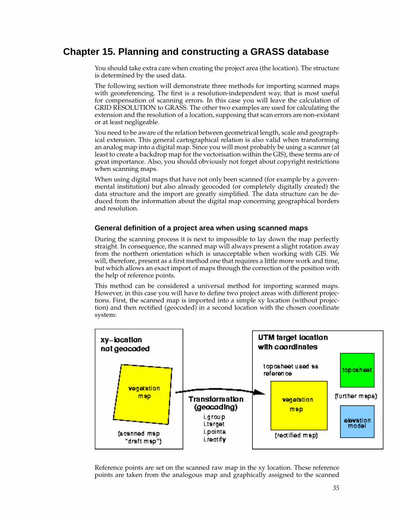
This method can be considered a universal method for importing scanned maps.However, in this case you will have to define two project areas with different projec-tions. First, the scanned map is imported into a simple xy location (without projec-tion) and then rectified (geocoded) in a second location with the chosen coordinatesystem:
Reference points are set on the scanned raw map in the xy location. These referencepoints are taken from the analogous map and graphically assigned to the scanned
35
Chapter 15. Planning and constructing a GRASS database
map. The next step is the geocoding of the scanned map through transformationfrom the xy location to the other location containing a projected coordinate system.Now the map is ready for GIS work.
Example: You have scanned a map at 300dpi. This map we call the “raw map”. Inthe Section called Definition of a project area with predefined geographical resolution youwill find the necessary calculation methods in order to determine the correct scan-ning parameters. It is useful to use a map which already provides marks at the crosssections of coordinate lines. These marks represent important coordinate points forthe rectification of the map. You should scan the map a few percentage points largerthan needed in GRASS later, so that the marks that are on the edge of the region ofinterest are clearly visible. Note : The edge of the paper is generally not parallel to thecoordinate lines of the projection system. This means that you cannot use the paperedges as location edges.
Before rectifying the raw map, you should first create the location in the actual projec-tion system you will be using for your map, with the required geographical bound-aries and resolution (see Chapter 16). Any projection supported by GRASS may beused. You should watch out that the resolution of the target location is not too lowsince that could cause the digital map to be quite illegible, depending on the scale.It is, therefore, worthwhile to begin by calculating the transformation between scan-ning resolution and geographical resolution.
Once the new location has been created, you have to leave GRASS again in order torestart it for the creation of the xy location (GRASS cannot switch between locationson-the-fly yet). Later, the rectification module will transfer the map that has beenimported into this xy location to the new location and adapt the orientation and theresolution according to the parameters of this projection.
Now the xy location needed for the scanned raw map has to be created. It has to havean extension of at least the number of pixels of the imported map in both directions(x and y). The resolution will be 1 pixel, as usual for xy locations . There actually isa relation to a geographical resolution (in meters, for example), but this relation isof no importance in a location without projection such as xy locations . The "real"resolution (that has been determined through the scanning resolution and the mapscale) is relevant only during the transformation into the new projection location .
If the map can only be scanned in several parts due to its size, all map parts are toimport into the same xy location . This xy location has to be created large enough inorder to hold all parts, i.e. you will have to choose its size according to the largestscanned map part. Since locations sizes can be freely chosen in GRASS, you can de-fine an even larger location "just to be sure". To find out the size of your scannedraw map in pixels, you can use the ImageMagick program mentioned in the previoussection.
You should by now have created two locations : one xy location for the raw map andone projected location into which the raw map shall be rectified, i.e. geocoded. Youwill find the instructions on how to import and rectify the scanned map in Chapter28.
Definition of a project area with predefined geographical resolution
This method for the creation of a location supposes that the boundaries of the projectarea are known and the scan parameters have to be adapted for a map that is to bescanned (and that can be scanned with no or negligeable errors).
The number of raster cells in a location results from the length and width of theproject area as well as the resolution, chosen according to the required precision ofthe results resolution grid resolution (GRID RESOLUTION).
Example: Let the length of a square location be 1 km, with a wanted resolution of 5mper cell (GRID RESOLUTION). Thus:
1,000m/5m = 200 rows (or columns) => 200*200 raster cells36
Chapter 15. Planning and constructing a GRASS database
If, for example, a scan map is to be scanned for this region, it has to contain 200 x 200rows and columns in order to be imported without distortion. Therefore, in this case,it is the location that determines the scan resolution since the lenght and width of thescanned area are determined by the borders of the location . This is similar for anyother data whose resolution also has to be adapted (e.g. digital elevation model withdefined raster width).
Now we need to find out which resolution has to be used when scanning, in order toachieve this number of rows and columns at a fixed side length. In this example wewill assume a scale of 1:25000 on the map to be scanned. Thus, the location length of1000m becomes:
100,000cm/25,000 = 4cm,
i.e. 4cm on the map. The scanning resolution of this map that is to be imported iscalculated as follows:
raster rows (or columns) / side length of the map = 200 rows (or columns) / 4cm =50 rows / cm
In dpi (dots per inch, equivalent of rows or columns per inch) this becomes:
50 rows x 2.54 inches = 127dpi
This value has to be set in the scanner software, as well as the section of the mapthat corresponds to the geographical boundaries of the desired area that is to bescanned. Each map scale will result in a different resolution. The latter has to be cho-sen big enough in order to keep small map texts legible. While scanning, it is almostimpossible to achieve the exact number of rows and columns and a perfect orien-tation of the map. In this method, one is therefore obliged to rework the scannedmap with imaging software (as for example the netpbm-tools, which you can find athttp://netpbm.sourceforge.net/.
Now we will look at an alternative method for the definition of the project area de-pending on the data that is to be processed.
Definition of the project area without a previously defined resolution
This third method for creating a location is to be used when the resolution withinthe location location can be chosen freely in function of a scanned map (or any othergiven data). Here the parameters of the location are derived from the data. scanningThe image to be imported and the location must have the same number of rasterrows and columns. You can find out these values with the help of the ImageMagickprogram, available at http://www.imagemagick.org/. Use its identify command oropen the scanned map, right-click on it and chose "Image Info".
Which distance in nature corresponds to which length of a raster cell is determinedby the chosen scanning resolution. This values needs to be entered as the GRID RES-OLUTION during the creation of the location (see coordinates entry form on pagelocationform ). It is important not to change the image size since that would alter thescales within the image.
It is recommended to work with a scanning resolution somewhere between 150 and300 dpi (color image with 256 colors), with labels on the map being legible. The rasterresolution within GRASS (GRID RESOLUTION of the location is derived from that.Here is an example of how to calculate the resolution of a square location . Let usassume a scanning resolution of 300dpi:
300dpi = 300 rows / 2.54cm = 118.11 rows/cm
Let the scale of the scanned map be 1:25,000. Thus, one centimeter on the map isequivalent to 25,000cm in nature. Now let us calculate which distance in nature cor-responds to the length of a raster cell:
distance in nature / scanned rows per cm = 25,000cm / 118.11 rows = 211.6 cm/row= 2.12 m/row
37

Chapter 15. Planning and constructing a GRASS database
This value of 2.12m has to be entered as GRID RESOLUTION Grid resolution duringthe creation of the location . If you want the GRID resolution to be a whole number,you have to calculate backwards and change the scan resolution respectively. Nor-mally, you should be able to chose this resolution freely up to a maximum value.
Notes1. http://netpbm.sourceforge.net/
2. http://www.imagemagick.org/
38
Chapter 16. Set-up your location
To specify your new location gather out the following information:
• coordinate system for your project area (plane or with projection and ellipsoid)
• minimum and maximum coordinates of the area of interest
• ground resolution
The supported common coordinate systems are here1.
In general, planning of a database in a Geographical Information System requiressome preparation. The user should proceed with care, since the chosen data struc-ture determines the usability of the GIS. Special attention should be accorded to theresolution -- a high raster resolution requires large calculation and memory capaci-ties, a low raster resolution rarely provides acceptable results (this resolution issue isnot relevant for vector and sites data). The optimum is somewhere in between anddepends on the needs, but also a lot on the input data quality.
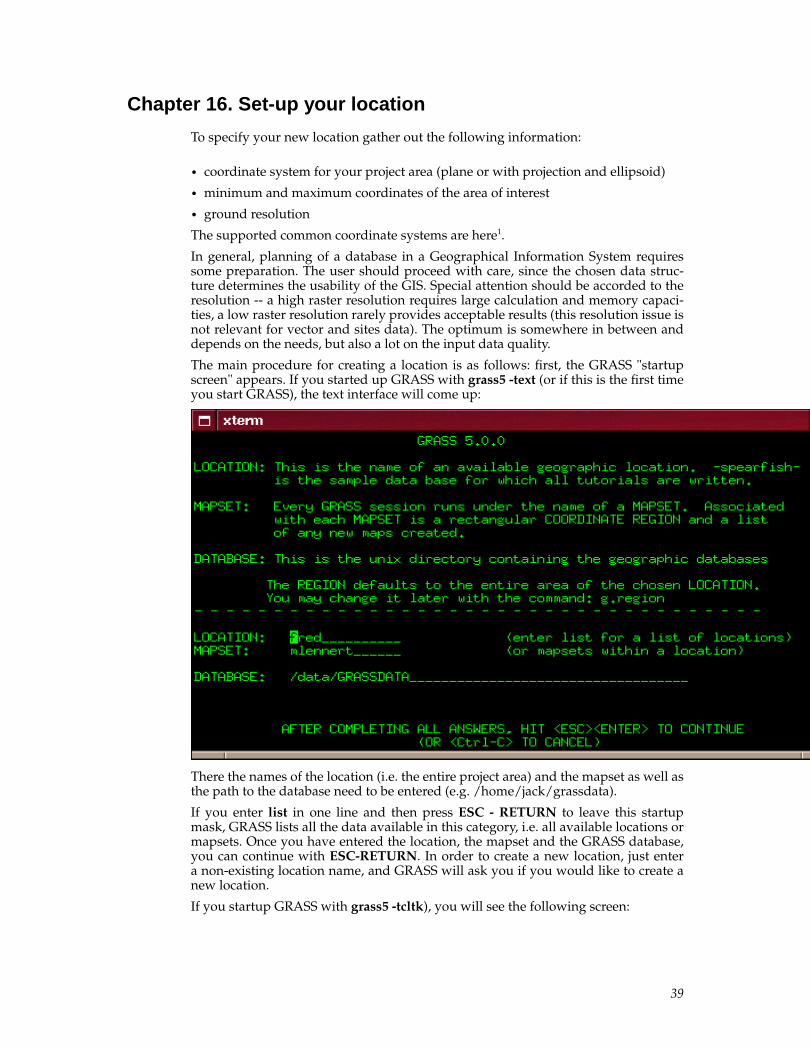
The main procedure for creating a location is as follows: first, the GRASS "startupscreen" appears. If you started up GRASS with grass5 -text (or if this is the first timeyou start GRASS), the text interface will come up:
There the names of the location (i.e. the entire project area) and the mapset as well asthe path to the database need to be entered (e.g. /home/jack/grassdata).
If you enter list in one line and then press ESC - RETURN to leave this startupmask, GRASS lists all the data available in this category, i.e. all available locations ormapsets. Once you have entered the location, the mapset and the GRASS database,you can continue with ESC-RETURN. In order to create a new location, just entera non-existing location name, and GRASS will ask you if you would like to create anew location.
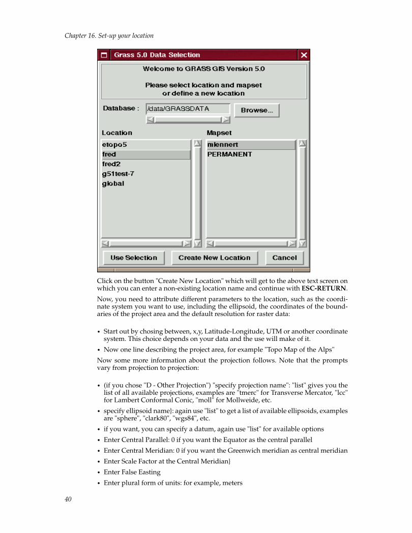
If you startup GRASS with grass5 -tcltk), you will see the following screen:
39
Chapter 16. Set-up your location
Click on the button "Create New Location" which will get to the above text screen onwhich you can enter a non-existing location name and continue with ESC-RETURN.
Now, you need to attribute different parameters to the location, such as the coordi-nate system you want to use, including the ellipsoid, the coordinates of the bound-aries of the project area and the default resolution for raster data:
• Start out by chosing between, x,y, Latitude-Longitude, UTM or another coordinatesystem. This choice depends on your data and the use will make of it.
• Now one line describing the project area, for example "Topo Map of the Alps"
Now some more information about the projection follows. Note that the promptsvary from projection to projection:
• (if you chose "D - Other Projection") "specify projection name": "list" gives you thelist of all available projections, examples are "tmerc" for Transverse Mercator, "lcc"for Lambert Conformal Conic, "moll" for Mollweide, etc.
• specify ellipsoid name}: again use "list" to get a list of available ellipsoids, examplesare "sphere", "clark80", "wgs84", etc.
• if you want, you can specify a datum, again use "list" for available options
• Enter Central Parallel: 0 if you want the Equator as the central parallel
• Enter Central Meridian: 0 if you want the Greenwich meridian as central meridian
• Enter Scale Factor at the Central Meridian}
• Enter False Easting
• Enter plural form of units: for example, meters
40
Chapter 16. Set-up your location
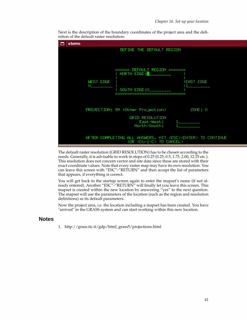
Next is the description of the boundary coordinates of the project area and the defi-nition of the default raster resolution:
The default raster resolution (GRID RESOLUTION) has to be chosen according to theneeds. Generally, it is advisable to work in steps of 0.25 (0.25, 0.5, 1.75, 2.00, 12.25 etc.).This resolution does not concern vector and site data since these are stored with theirexact coordinate values. Note that every raster map may have its own resolution. Youcan leave this screen with “ESC”-“RETURN” and then accept the list of parametersthat appears, if everything is correct.
You will get back to the startup screen again to enter the mapset’s name (if not al-ready entered). Another “ESC”-“RETURN” will finally let you leave this screen. Thismapset is created within the new location by answering “yes” to the next question.The mapset will use the parameters of the location (such as the region and resolutiondefinitions) as its default parameters.
Now the project area, i.e. the location including a mapset has been created. You have"arrived" in the GRASS system and can start working within this new location.
Notes1. http://grass.itc.it/gdp/html_grass5/projections.html
41

Chapter 16. Set-up your location
42
Chapter 17. Manage your data
Different commands allow you to list, copy, rename or erase data within the currentlocation..
• g.list1: Lists available GRASS data base files of the user-specified data type to stan-dard output.
• g.rename2: Renames data base element files in the user’s current mapset.
• g.copy3: Copies available data files in the user’s current mapset search path andlocation to the appropriate element directories under the user’s current mapset.
• g.remove4: Removes data base element files from the user’s current mapset.
If you wish to deal with an entire location you will have to do so by hand, after havingleft GRASS.
• In order to remove a location with the name "location_name", go to the directorythat contains this location (i.e. the GRASS database directory) and use the com-mand rm -rf location_name. This will irrevocably erase all the data, so be careful!
• In order to copy a location with the name "location_name" to another directoryor another machine, go to the GRASS database directory and use the commandtar cvf location_name.tar location_name to package the entire directory into onefile. You should then compress this file with gzip location_name.tar or bzip2 loca-tion_name.tar. Copy the resulting file to the new location. Be aware, however thatuser and group settings (gid and uid) might get mangled, so be prepared to changethose with chown.
In order to access maps within the same location, but in another mapset, you have toset your mapset search path. If you do not wish some of your data to be accessiblefor everyone, you can limit the access to a particular mapset you own.
• g.mapsets5: Modifies the user’s current mapset search path, affecting the user’saccess to data existing under the other GRASS mapsets in the current location.
• g.access6: Control access to the current mapset.
Notes1. http://grass.itc.it/gdp/html_grass5/html/g.list.html
2. http://grass.itc.it/gdp/html_grass5/html/g.rename.html
3. http://grass.itc.it/gdp/html_grass5/html/g.copy.html
4. http://grass.itc.it/gdp/html_grass5/html/g.remove.html
5. http://grass.itc.it/gdp/html_grass5/html/g.mapsets.html
6. http://grass.itc.it/gdp/html_grass5/html/g.access.html
43

Chapter 17. Manage your data
44

Chapter 18. Supported formats
Import modules1
Export modules2
Notes1. http://grass.itc.it/gdp/html_grass5/import.html
2. http://grass.itc.it/gdp/html_grass5/export.html
45

Chapter 18. Supported formats
46
Chapter 19. Raster Import
The module r.in.gdal1 offers a common interface for many different raster formats2.Try this first, especially since it also offers such practical options as on-the-fly locationcreation or extension of the default region in order to adapt it to the imported file.
If r.in.gdal does not suit your needs, use the appropriate r.in.* module3 (replace the *with the name of the format you wish to import).
After the import, you will probably want to run r.support4 in order to modify orcreate the GRASS support files.
For importing scanned maps, you will need to create a x,y-location according to theinstructions in Chapter 15, scan the map in the desired resolution and save it into anappropriate raster format (e.g. tiff, jpeg, png, pbm) and then use r.in.gdal to importit. You will probably have to recify it in order to obtain geocoded data. Chapter 28contains more information about this process.
Notes1. http://grass.itc.it/gdp/html_grass5/html/r.in.gdal.html
2. http://www.remotesensing.org/gdal/formats_list.html
3. http://grass.itc.it/gdp/html_grass5/raster.html
4. http://grass.itc.it/gdp/html_grass5/html/r.support.html
47

Chapter 19. Raster Import
48
Chapter 20. Vector Import
For vector import use the appropriate v.in.* module1 (replace the * with the name ofthe format you wish to import). There is no common interface for different formats(yet).
After the import, you have to run v.support2 in order to build the relevant GRASSsupport files. Some of the vector import modules run this automatically for you, socheck the relevant man page.
Notes1. http://grass.itc.it/gdp/html_grass5/vector.html
2. http://grass.itc.it/gdp/html_grass5/html/v.support.html
49

Chapter 20. Vector Import
50

Chapter 21. Sites (point data) import
The easiest way to profit from the new multi-dimension and multi-attribute site for-mat in GRASS 5.0 is to create the file yourself. You can find details about the for-mat in the s.in.ascii1 man page. Once you have created the file, you can "import"it into GRASS by copying it directly into your mapset: cp NameOfYourSitesFile$GISDBASE/$LOCATION_NAME/$MAPSET/site_lists/ (you have to be in a run-ning GRASS session for this command to work).
For site import from other formats use the appropriate s.in.* module2 (replace the *with the name of the format you wish to import).
Notes1. http://grass.itc.it/gdp/html_grass5/html/s.in.ascii.html
2. http://grass.itc.it/gdp/html_grass5/sites.html
51

Chapter 21. Sites (point data) import
52
Chapter 22. Managing GRASS Monitors
GRASS map display windows are no “normal” windows. Rather, they display geo-graphical data with coordinates. These windows are called "monitors" in GRASS andare managed with the d.mon1 command or through the Display->Monitors menu inTclTkGRASS.
You can open several different monitors at once. Use d.mon start= to start the moni-tor of your choice and d.mon select= to select the monitor you want to display dataon next. To stop a monitor, use d.mon stop= or simply click on the closing button pro-vided by your window manager. You can also resize a monitor the way you wouldresize any window in your window manager.
Frames in monitors
GRASS offers the possibility to divide a monitor into several distinct frames. Thisgives you the opportunity to create a more sophisticated layout of your maps andother data. For example, you can create a frame for header information (title, date,etc), a frame for the actual map, a frame for footer information (author, sources, etc),a frame for the legend, etc, etc. The module for frame creation is d.frame2 and it isquite simple to use (see the manual page for details):
d.frame -c frame=title at=90,100,0,100 # create a title frameecho "TITRE" | d.text -b size=75 at=45,30 # write the title into the title framed.frame -c frame=map at=10,90,0,100 # create a map framed.rast combel # draw a raster map into that framed.vect autoroute col=violet # draw a vector map into the same framed.frame -c frame=legend at=0,10,0,100 # create a legend frameecho "Cartography: M. Lennert" | d.text size=20 at=75,50 # draw text in the legend framed.barscale at=10,920 # create a barscale in the legend frame
Notes1. http://grass.itc.it/gdp/html_grass5/html/d.mon.html
2. http://grass.itc.it/gdp/html_grass5/html/d.frame.html
53

Chapter 22. Managing GRASS Monitors
54
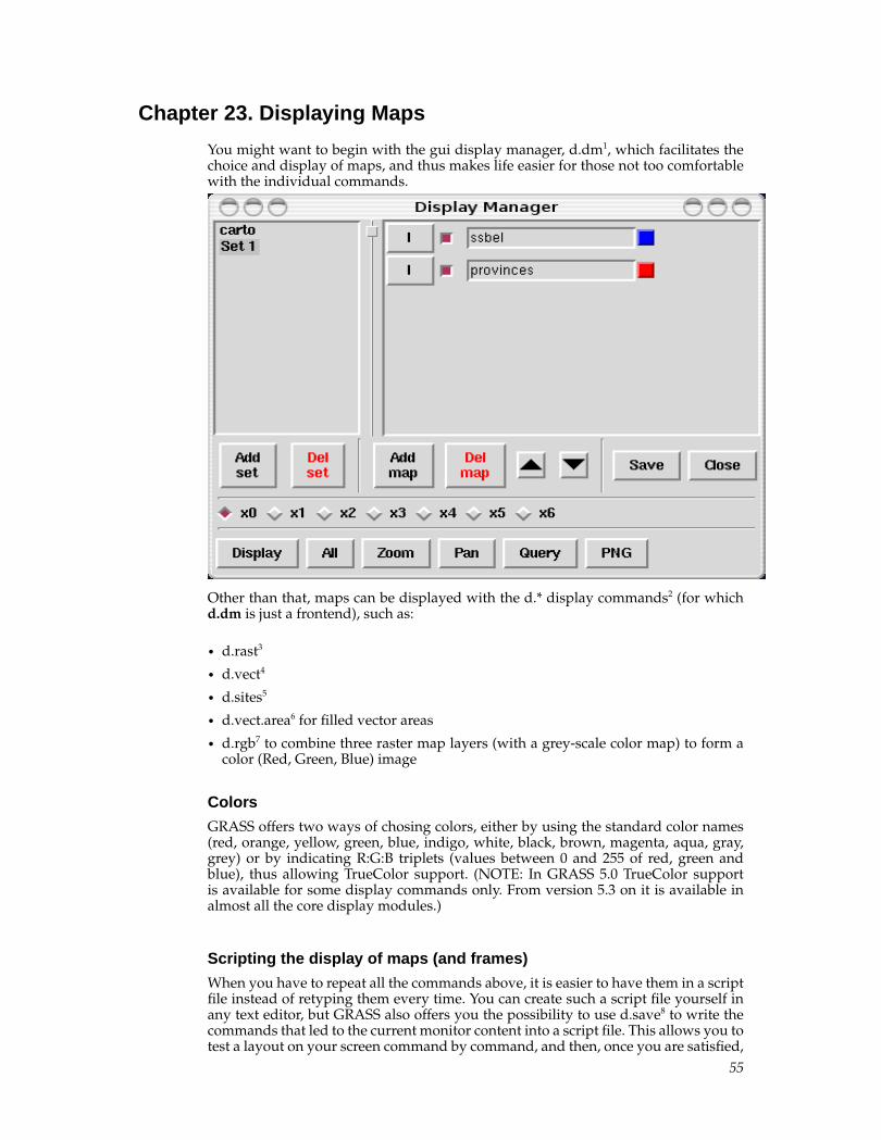
Chapter 23. Displaying Maps
You might want to begin with the gui display manager, d.dm1, which facilitates thechoice and display of maps, and thus makes life easier for those not too comfortablewith the individual commands.
Other than that, maps can be displayed with the d.* display commands2 (for whichd.dm is just a frontend), such as:
• d.rast3
• d.vect4
• d.sites5
• d.vect.area6 for filled vector areas
• d.rgb7 to combine three raster map layers (with a grey-scale color map) to form acolor (Red, Green, Blue) image
Colors
GRASS offers two ways of chosing colors, either by using the standard color names(red, orange, yellow, green, blue, indigo, white, black, brown, magenta, aqua, gray,grey) or by indicating R:G:B triplets (values between 0 and 255 of red, green andblue), thus allowing TrueColor support. (NOTE: In GRASS 5.0 TrueColor supportis available for some display commands only. From version 5.3 on it is available inalmost all the core display modules.)
Scripting the display of maps (and frames)
When you have to repeat all the commands above, it is easier to have them in a scriptfile instead of retyping them every time. You can create such a script file yourself inany text editor, but GRASS also offers you the possibility to use d.save8 to write thecommands that led to the current monitor content into a script file. This allows you totest a layout on your screen command by command, and then, once you are satisfied,
55

Chapter 23. Displaying Maps
to save this layout into a file. This is especially useful for cartography (see Part XIIIin Grass Tutorial).
Notes1. http://grass.itc.it/gdp/html_grass5/html/d.dm.html
2. http://grass.itc.it/gdp/html_grass5/display.html
3. http://grass.itc.it/gdp/html_grass5/html/d.rast.html
4. http://grass.itc.it/gdp/html_grass5/html/d.vect.html
5. http://grass.itc.it/gdp/html_grass5/html/d.sites.html
6. http://grass.itc.it/gdp/html_grass5/html/d.vect.area.html
7. http://grass.itc.it/gdp/html_grass5/html/d.rgb.html
8. http://grass.itc.it/gdp/html_grass5/html/d.save.html
56

Chapter 24. Zooming and Panning
Use d.zoom1 for zooming and panning in the currently selected monitor. d.zoomwithout any command line options allows you to zoom in by selecting a zoomingframe (left mouse button) or to zoom out (middle mouse button). If you launchd.zoom -f, you get the option between zooming (left mouse button) or panning (mid-dle mouse button). If you only want to pan, try d.pan2.
Both d.zoom and d.pan change your current region settings. They are, in that sense,an interactive version of g.region3, so be aware that any command using the currentregion settings will be affected by the use of d.zoom or d.pan.
Notes1. http://grass.itc.it/gdp/html_grass5/html/d.zoom.html
2. http://grass.itc.it/gdp/html_grass5/html/d.pan.html
3. http://grass.itc.it/gdp/html_grass5/html/g.region.html
57

Chapter 24. Zooming and Panning
58
Chapter 25. Adding Legends and Scales
Legends in GRASS only exist for raster maps. Currently, GRASS does not supportlegends for vector maps such as those drawn with d.vect.area1.
See the module d.legend2 for your legends. (This module is in active developmentfor the moment, so its usability should continue to be enhanced in the near future.)You can use d.legend to display a legend in the same monitor as the map, or in adifferent monitor (use d.mon3 to start and/or select a different monitor). Through its"-m" option d.legend allows you to place and size the legend with the mouse.
Currently d.barscale4 is your best choice for placing a barscale on your map, includ-ing a small north arrow. If you would prefer a simple line instead of a barscale, youcan use d.scale5 (NOTE: this is depreciated as of GRASS 5.3, d.barscale -l does thesame thing, only better). However, the latter does not survive a zoom or pan, whilethe former does. Furthermore, d.barscale also gives you the choice of feet/miles in-stead of meters.
Notes1. http://grass.itc.it/gdp/html_grass5/html/d.vect.area.html
2. http://grass.itc.it/gdp/html_grass5/html/d.legend.html
3. http://grass.itc.it/gdp/html_grass5/html/d.mon.html
4. http://grass.itc.it/gdp/html_grass5/html/d.barscale.html
5. http://grass.itc.it/gdp/html_grass5/html/d.scale.html
59

Chapter 25. Adding Legends and Scales
60

Chapter 26. Visualize in 3D with nviz
For a tutorial on the use of nviz, the 3D visualization program for GRASS, see here1.For some examples of what can be done with nviz, see here2.
Notes1. http://grass.itc.it/gdp/nviz/nviz_tut.html
2. http://grass.itc.it/gdp/nviz/index.html
61

Chapter 26. Visualize in 3D with nviz
62
Chapter 27. Digitizing Vector Maps
There are two ways of vectorizing maps (AKA digitizing):
• using a digitizer,
• digitizing on-screen.
In the first case the map is placed on the digitizer, the corners are selected by a mouseclick and the respective coordinates entered through the keyboard. This process iscalled "’registering a map"’. The advantage of this method is that the user is alwaysin control of the whole map. However, the high price of the equipment and the lackof magnification capabilities, e.g. for low-quality maps, are significant disadvantages.Furthermore, the map must not show any signs of lateral stretch to prevent wrongsite coordinates.
On-screen digitizing requires a scanned and geocoded raster map (image) that is dis-played on a GRASS monitor. All relevant map objects will be vectorized using themouse. It is not necessary to register such a map as it is geocoded already. The ad-vantage of this method is the support of zooming, hence an improved accuracy canbe achieved. Apart from access to a scanner no financial input is required. However,the disadvantage of this method lies in the somewhat awkward orientation on themap on the screen.
Rules for Digitizing in Topological GIS
There are a few basic rules regarding digitizing from analogue maps that apply totopological GIS, such as GRASS. Obedience to these rules is essential in order to usethe topological features of the software.
• Lines must not cross without nodes.
• Lines that use common "node" must hit it exactly. Make use of the snapping func-tion of the digitizing module.
• Common area boundaries must only be digitized once.
• Areas must be closed. Use the snapping function of the digitizing module.
• Store lines and areas in separate maps to avoid problems with crossing lines. It isalso easier to assign a certain type (line or area boundary) to a line.
There should not be any problems when all the rules are fulfilled.
Digitizing Maps
If there is no digitizer available but a scanner, it is still easy to digitize a map. You canfind information on importing a scanned map into GRASS in Chapter 19 and Chapter28.
You can use your mouse for digitizing instead of a digitizer. After starting aGRASS monitor, run the module v.digit1 (in tcltkgrass chose ’Vector->Developmap->Digitize’)to change the settings from digitizer to mouse. Choose digitizer"’none"’. After selecting a new or existing vector file you will see a dialoguerequesting project data. It is necessary to change the parameter "’Map’s scale"’ from1:0 to the respective scale of the map:
Provide the following information:
Your organization Geographisches Institut_____Todays date (mon,yr) Jan 25 99__________Your name Emil______________Maps name realnutzung____________________________
63
Chapter 27. Digitizing Vector Maps
Maps date __________Maps scale 1:25000____Other info Sommer 1998____________________________Zone 0____West edge of area 3568750_______South edge of area 5762774_______East edge of area 3574250_______North edge of area 5767726_______
After completing this dialogue you will be transferred to the main menu.
In order to digitize on the basis of the scanned raster map, place it in the background:Choose "Backdrop cell map" (’B’) from the "Customize" menu (’C’). This will load theraster map to the background.
Now you can open the digitizing menu by pressing ’D’. The module v.digit2 is some-what self-explanatory, for more specific information please refer to the CERL v.digittutorial (pdf file)3. The ’Color’ menu under ’Customize’ allows you to change thecolors of the digitized objects (lines, areas). This allows for optimized color coding.It is important to choose the appropriate type of object (area, line, site) by pressing’t’. If necessary, switch on the ’auto labelling function’. This function assigns the cat-egory number, however, it is not (yet) possible to enter the category text in v.digit.Because of this you should write down which category number belongs to which ob-ject. Run the module v.support4 to enter the category labels (’Edit the category file’-in tcltkgrass chose ’Vector->Develop map->Edit vector categories’).
Make use of the ’zoom function to improve your accuracy significantly.
To avoid confusion: Points may be saved as vectors or in GRASS sites format. Vectorsare usually the result of digitizing, points in the GRASS format result from files withcoordinates (N,E) and attributes.
Again, it is an important rule to digitize boundaries of adjacent areas only once.GRASS automatically assigns this boundary to both areas. Never digitize two par-allel lines!
Digitizing Areas
Digitizing areas is generally a bit harder and requires more practice. For this reasonwe will explain setting of attributes in more detail. Choose the vector types in the’Digitize’ menu of the v.digit module.
Press ’t’ to toggle the type between:
• LINE,
• AREA EDGE,
• SITE.
It is mandatory to close areas because only then you can create the GIS vector topol-ogy and assign label points. Since it is nearly impossible to hit line ends exactly, thesnapping function allows the closing of areas:
64
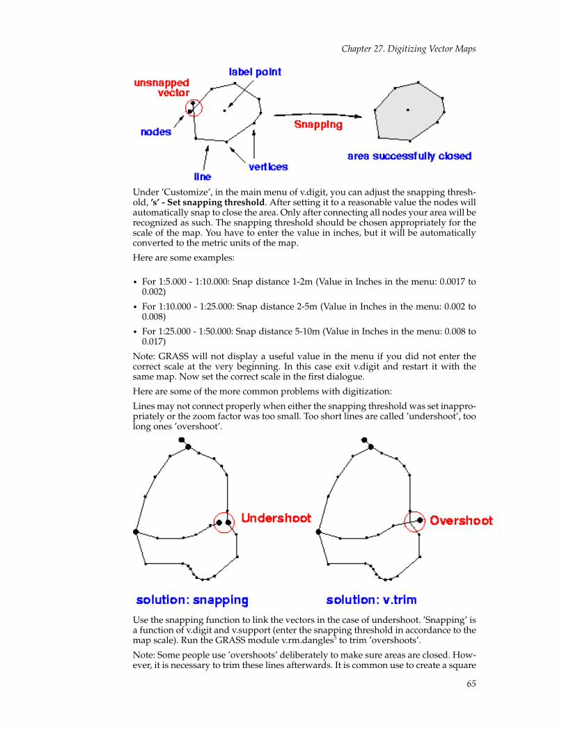
Chapter 27. Digitizing Vector Maps
Under ’Customize’, in the main menu of v.digit, you can adjust the snapping thresh-old, ’s’ - Set snapping threshold. After setting it to a reasonable value the nodes willautomatically snap to close the area. Only after connecting all nodes your area will berecognized as such. The snapping threshold should be chosen appropriately for thescale of the map. You have to enter the value in inches, but it will be automaticallyconverted to the metric units of the map.
Here are some examples:
• For 1:5.000 - 1:10.000: Snap distance 1-2m (Value in Inches in the menu: 0.0017 to0.002)
• For 1:10.000 - 1:25.000: Snap distance 2-5m (Value in Inches in the menu: 0.002 to0.008)
• For 1:25.000 - 1:50.000: Snap distance 5-10m (Value in Inches in the menu: 0.008 to0.017)
Note: GRASS will not display a useful value in the menu if you did not enter thecorrect scale at the very beginning. In this case exit v.digit and restart it with thesame map. Now set the correct scale in the first dialogue.
Here are some of the more common problems with digitization:
Lines may not connect properly when either the snapping threshold was set inappro-priately or the zoom factor was too small. Too short lines are called ’undershoot’, toolong ones ’overshoot’.
Use the snapping function to link the vectors in the case of undershoot. ’Snapping’ isa function of v.digit and v.support (enter the snapping threshold in accordance to themap scale). Run the GRASS module v.rm.dangles5 to trim ’overshoots’.
Note: Some people use ’overshoots’ deliberately to make sure areas are closed. How-ever, it is necessary to trim these lines afterwards. It is common use to create a square
65
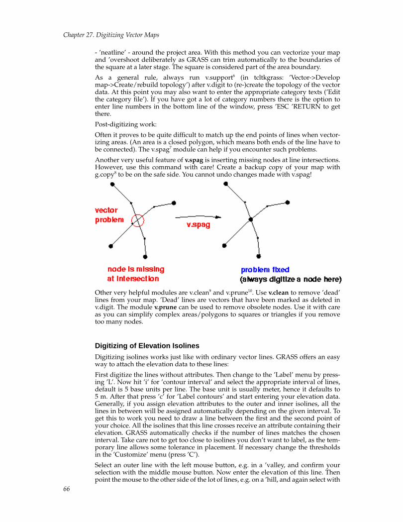
Chapter 27. Digitizing Vector Maps
- ’neatline’ - around the project area. With this method you can vectorize your mapand ’overshoot deliberately as GRASS can trim automatically to the boundaries ofthe square at a later stage. The square is considered part of the area boundary.
As a general rule, always run v.support6 (in tcltkgrass: ’Vector->Developmap->Create/rebuild topology’) after v.digit to (re-)create the topology of the vectordata. At this point you may also want to enter the appropriate category texts (’Editthe category file’). If you have got a lot of category numbers there is the option toenter line numbers in the bottom line of the window, press ’ESC ’RETURN to getthere.
Post-digitizing work:
Often it proves to be quite difficult to match up the end points of lines when vector-izing areas. (An area is a closed polygon, which means both ends of the line have tobe connected). The v.spag7 module can help if you encounter such problems.
Another very useful feature of v.spag is inserting missing nodes at line intersections.However, use this command with care! Create a backup copy of your map withg.copy8 to be on the safe side. You cannot undo changes made with v.spag!
Other very helpful modules are v.clean9 and v.prune10. Use v.clean to remove ’dead’lines from your map. ’Dead’ lines are vectors that have been marked as deleted inv.digit. The module v.prune can be used to remove obsolete nodes. Use it with careas you can simplify complex areas/polygons to squares or triangles if you removetoo many nodes.
Digitizing of Elevation Isolines
Digitizing isolines works just like with ordinary vector lines. GRASS offers an easyway to attach the elevation data to these lines:
First digitize the lines without attributes. Then change to the ’Label’ menu by press-ing ’L’. Now hit ’i’ for ’contour interval’ and select the appropriate interval of lines,default is 5 base units per line. The base unit is usually meter, hence it defaults to5 m. After that press ’c’ for ’Label contours’ and start entering your elevation data.Generally, if you assign elevation attributes to the outer and inner isolines, all thelines in between will be assigned automatically depending on the given interval. Toget this to work you need to draw a line between the first and the second point ofyour choice. All the isolines that this line crosses receive an attribute containing theirelevation. GRASS automatically checks if the number of lines matches the choseninterval. Take care not to get too close to isolines you don’t want to label, as the tem-porary line allows some tolerance in placement. If necessary change the thresholdsin the ’Customize’ menu (press ’C’).
Select an outer line with the left mouse button, e.g. in a ’valley, and confirm yourselection with the middle mouse button. Now enter the elevation of this line. Thenpoint the mouse to the other side of the lot of lines, e.g. on a ’hill, and again select with
66
Chapter 27. Digitizing Vector Maps
the left mouse button, confirm with the middle one and enter its elevation. Now thesetwo lines are connected by a straight line that crosses all the isolines in between. Allthese lines automatically get assigned the appropriate value. In the case the choseninterval and the number of lines do not match GRASS will display an error (warning)message and stop the process. If this happens please count again or choose smallersteps.
Notes1. http://grass.itc.it/gdp/html_grass5/html/v.digit.html
2. http://grass.itc.it/gdp/html_grass5/html/v.digit.html
3. http://grass.itc.it/gdp/vector/digit.pdf
4. http://grass.itc.it/gdp/html_grass5/html/v.support.html
5. http://grass.itc.it/gdp/html_grass5/html/v.rm.dangles.html
6. http://grass.itc.it/gdp/html_grass5/html/v.support.html
7. http://grass.itc.it/gdp/html_grass5/html/v.spag.html
8. http://grass.itc.it/gdp/html_grass5/html/g.copy.html
9. http://grass.itc.it/gdp/html_grass5/html/v.clean.html
10. http://grass.itc.it/gdp/html_grass5/html/v.prune.html
67

Chapter 27. Digitizing Vector Maps
68
Chapter 28. Processing Scanned Maps
In order to process a scanned map, you first have to import it, probably withr.in.gdal1, into an x,y-location, prepared according to the calculations in Chapter 15.Then you can rectify it in order to obtain geocoded data.
Don’t forget to use g.region2 to make sure your map is correctly displayed andtreated: g.region rast=NameOfYourRasterMap.
In this section the rectification of a scanned map to its topographic reference willbe explained. For better understanding you should read the Section called Generaldefinition of a project area when using scanned maps in Chapter 15.
Commonly such files are stored in TIFF, PNG or other formats. The amount of rowsand columns can be set in the scanning software used, or obtained through theImageMagick identify command.
Start GRASS with an xy location which has been set up according to the size of thescanned map, and import it as described earlier. The scanned map will now be trans-formed by an affine transformation (with the i.rectify3 module4 The affine transfor-mation rotates, stretches and contracts, and is usable for raster data, for which theinternal orientation should be kept.
Geocoding of scanned maps
Now the "rectification" of the raw map, i.e. its transformation for geocoding, will beperformed. The process explained here is valid for scanned, unreferenced data only.We will use the modules i.rectify5, i.points6, and i.target7 modules.
69
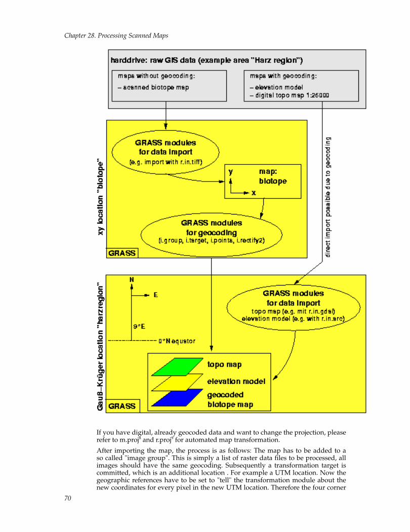
Chapter 28. Processing Scanned Maps
If you have digital, already geocoded data and want to change the projection, pleaserefer to m.proj8 and r.proj9 for automated map transformation.
After importing the map, the process is as follows: The map has to be added to aso called "image group". This is simply a list of raster data files to be processed, allimages should have the same geocoding. Subsequently a transformation target iscommitted, which is an additional location . For example a UTM location. Now thegeographic references have to be set to "tell" the transformation module about thenew coordinates for every pixel in the new UTM location. Therefore the four corner
70
Chapter 28. Processing Scanned Maps
coordinates in the xy location are assigned geographical coordinates. These are, ofcourse, the geographical corners, not map sheet paper corners! If there are no read-able map borders present, e.g. you have scanned only a cut of the map, you can usethe corner points of printed reference crosses. These should be chosen as close aspossible towards the "real" corners of the map. These points have to enclose a rectan-gular area, as the cut will be turned, stretched and contracted in the following affinetransformation.
If no reference crosses are available either, use well identifiable features, such as roadintersections. Once the geographic references are assigned, the transformation of theraw map into the UTM location is performed. The process in detail is as follows:
a. Prompt the name of the newly to be set up image group: $ i.group
• Name this group, for example: "map1".
• Mark the map to be imported with a "x".
• Leave module i.group with "return".
b. Indicate the target location and mapset (into which the UTM location shouldbe transformed) in: $ i.target
c. Start a GRASS monitor: $ d.mon x0
d. Assign the UTM coordinates to the four corner points of the image to be trans-formed: $ i.points
• Prompt the image group to be transformed (contains only the map), in thisexample "map1".
• Change to the GRASS monitor. Here display the imported map.
• Using the mouse, select as precisely as possible the first reference cross (firstcorner point of the image to be transformed). Enter the related UTM coor-dinate at the command line (the related easting and northing, as taken fromthe printed map), delimited by blanks. The "ZOOM" function is quite usefulfor this, allowing to find the matching points more easily.
With help of the "Analyze" component you can check the "rms error".10 Itshould not be higher than the GRID RESOLUTION of the UTM-location. Allpartial errors (one for every matching point) are added up into an over allerror. Is this one to large, you can adjust it with resetting and reassigningof single matching points. In the "Analyzes" window double click the pointconcerned for to delete it. Afterwards reassign it to reduce the "rms error".Are all four points assigned sufficiently correct, leave $ i.points , all assigna-tions will be saved automatically.
e. Now start the transformation module: $i.rectify with a 1st grade polynom (as"order of transformation""). This will perform the linear transformation.
First the image group to be transformed (in this case: "map1") and the name ofthe new file(s) are prompted. Now choose "1" as the "order of transformation".Finally you will be asked if you want to transform into
a. the current location or
b. the "minimal region".
Here you must choose menu point (1.), which is equivalent to the completeUTM location . Otherwise only the current active part of the UTM locationwould be transformed, which could be a cut of the complete area.
71
Chapter 28. Processing Scanned Maps
The computation time for an A4 size map (21x29,7cm) scanned with 300dpi ison a SUN SPARC/25 close to five minutes. A Linux PC (above 200MHz) worksfaster.
As UNIX is capable of multitasking, you can go on working with GRASS, or evenleave it, while the computation runs in the background. After the transformation hasfinished (i.rectify sends an email then), the success should be checked in the target-location (if you did not do it yet, leave and restart GRASS now: exit the xy locationand start it again in the UTM location ). After starting a GRASS monitor the trans-formed map can be displayed with d.rast11.
The d.what.rast12 module allows in combination with the magnification of single mapareas (see Chapter 24), to check the coordinates of the reference crosses. These should,of course, correlate with the equivalent ones on the printed map. Otherwise the "rmserror" was probably too high. Correcting is possible by reassigning single points inthe xy location. In this case the transformed map in the UTM location should bedeleted (with r.remove13), as it will be remade in the new transformation. Subse-quently transform with i.rectify14 as described above. The result should, again, bechecked. If the transformation was successfull, then the xy location, which is nownot needed anymore, can be deleted (see Chapter 17 for how to do this).
Gap free geocoding of multiple, adjacent, scanned maps
The transformation described in the preceding section can be used for importing sev-eral adjacent scanned maps without gaps. Access to drum scanners will exist only inrare cases, but normal maps are to large for customary scanners.
A usable solution is the scanning of maps in multiple parts. This solution requiressome more expense, but spares the purchase of an expensive scanner (large scalescanner). It is very important to scan with overlapping borders, as this will improvethe fixing of matching points.
As described above, a target location has to be set up in the target coordinate system,large enough to cover the complete area to be scanned. The resolution should bechosen sufficiently high to display the smallest conventional sign.
All scanned raw maps are imported into the xy location subsequently. Please payattention to the fact, that the extent of the xy location has to be equal to the extent ofthe complete area to be scanned.
Now open an image group for every imported map (even if it contains only one map),and adjust the transformation target for all of them to the UTM location (modulesi.group15 and i.target16). The following process:
Each of the four corner coordinates of the raw maps to be transformed is assigned aUTM coordinate pair (i.points17), see preceding section). These points must surrounda rectangular area, as this area will be turned and resized with the affine transforma-tion. With i.rectify18 (as 1st grade polynom) the according map will be transformedinto the UTM system.
Do the same with all the other maps in the xy location.
Once all scanned maps are transformed, the result can be checked in the UTM loca-tion (for that you will have to leave the xy location). Restart GRASS and choose theUTM project area. Now all individual maps should be checked for their correct posi-tioning and orientation (base accuracy). Open a GRASS monitor and put the regionto maximum (default value): g.region -d19
Afterwards it is absolutely necessary to run d.erase20, to inform the graphical subsys-tem of the changed coordinates. With starting d.rast21 without parameter (interactivemode) you have the possibility (after choosing the file to display) to overlay rasterimages (overlay mode: "yes" or flag "-o"). This way each file gets displayed after eachother, and the maps should lie next to each other. With d.zoom22 you can now inspect
72
Chapter 28. Processing Scanned Maps
if there are any gaps between the maps (redisplaying with d.rast is necessary). Ideallythere are no gaps to be seen.
If the maps show any unwanted borders, these can easily removed. To do so, zoomedinto the map with d.zoom23 and adjust the new coordinates with g.region24 in smallsteps to reach "comfortable", rounded values. Here you can also use the "-a" flag incombination with "res=" parameter of g.region25 to align the map boundaries withrespect to the desired resolution. In order to save the map at the new size, generate a"self copy" of the displayed map portion with r.mapcalc26:
mapcalc> new_map = old_map
Notes1. http://grass.itc.it/gdp/html_grass5/html/r.in.gdal.html
2. http://grass.itc.it/gdp/html_grass5/html/g.region.html
3. http://grass.itc.it/gdp/html_grass5/html/i.rectify.html
4. The affine transformation is a linear transformation, the parameters of whichare calculated through regression analysis. The "nearest neighbor resampling"method is used by i.rectify during the transformation.
5. http://grass.itc.it/gdp/html_grass5/html/i.rectify.html
6. http://grass.itc.it/gdp/html_grass5/html/i.points.html
7. http://grass.itc.it/gdp/html_grass5/html/i.target.html
8. http://grass.itc.it/gdp/html_grass5/html/m.proj.html
9. http://grass.itc.it/gdp/html_grass5/html/r.proj.html
10. The "rms error" represents the distance of the matching point from ideally placedmatching point. It is calculated through: rms = ((x-x orig )^2 + (y-y orig ))^(1/2)
11. http://grass.itc.it/gdp/html_grass5/html/r.rast.html
12. http://grass.itc.it/gdp/html_grass5/html/d.what.rast.html
13. http://grass.itc.it/gdp/html_grass5/html/g.remove.html
14. http://grass.itc.it/gdp/html_grass5/html/i.rectify.html
15. http://grass.itc.it/gdp/html_grass5/html/i.group.html
16. http://grass.itc.it/gdp/html_grass5/html/i.target.html
17. http://grass.itc.it/gdp/html_grass5/html/i.points.html
18. http://grass.itc.it/gdp/html_grass5/html/i.rectify.html
19. http://grass.itc.it/gdp/html_grass5/html/g.region.html
20. http://grass.itc.it/gdp/html_grass5/html/d.erase.html
21. http://grass.itc.it/gdp/html_grass5/html/d.rast.html
22. http://grass.itc.it/gdp/html_grass5/html/d.zoom.html
23. http://grass.itc.it/gdp/html_grass5/html/d.zoom.html
24. http://grass.itc.it/gdp/html_grass5/html/g.region.html
25. http://grass.itc.it/gdp/html_grass5/html/g.region.html
26. http://grass.itc.it/gdp/html_grass5/html/r.mapcalc.html
73

Chapter 28. Processing Scanned Maps
74
Chapter 29. Raster Categories and Attributes
In the raster data model, cell category numbers can be one of two things: either theyare measurements of real-life surface values (light intensity in images, height in dig-ital terrain models, slope, temperature, etc) or they represent classes of categories(scanned maps, land use, soil types, etc). In the first case, labels are not very neces-sary since the type of map defines the type of values themselves, in the second, theyare indispensable in order to document the meaning of the category numbers.
In GRASS, the raster map is stored in a binary file which contains the category num-bers for each cell. The category labels are stored in a text file which contains the cate-gory numbers with their respective labels. This chapter will look at different aspectsof the management of categories.
Viewing category values
The first thing you might wish to do is see which category values are present in yourraster file. Here is a list of modules you can use for this purpose:
• r.cats1 : Prints category values and labels associated with user-specified raster maplayers
• r.describe2 : Prints terse list of category values found in a raster map layer
• r.what3 : Queries raster map layers on their category values and category labels
• d.what.rast4 : Allows the user to interactively (with the mouse) query the categorycontents of multiple raster map layers at user-specified locations within the currentgeographic region
• r.report5 : Reports statistics for raster map layers, by category
• r.stats6 : Generates area statistics for raster map layers (similar to r.report
• r.statistics7 : Category or object oriented statistics
• r.univar8 : Univariate statistics for a GRASS raster map
For more information on statistics and reports, see Chapter 33.
Changing category values
You have to distinguish between changing the category values of a map and changingthe category labels. Actually the first is not really possible without creating a newmap, dropping the old one and renaming the new one to the old one’s name. You cando the latter directly on a map.
In order to create a new map by changing the category values of an already existingone, you can use the following modules:
• r.reclass9 : Creates a new (pseudo-)map layer whose category values are basedupon the user’s reclassification of categories in an existing raster map layer
• r.recode10 : Creates an output map layer based on an input raster map layer
• r.rescale11 : Rescales the range of category values in a raster map layer (also seer.rescale.eq12 and r.rescale.inf13
• r.mapcalc14 : Raster map layer data calculator (see Chapter 36 for more detailedinformation)
• r.clump15 : Recategorizes data in a raster map layer by grouping cells that formphysically discrete areas into unique categories
For changing the category labels of a raster map, use r.support16. Enter ’y’ when youget to the question "Edit the category file for [mapname]?". You will get to a screen
75
Chapter 29. Raster Categories and Attributes
showing the highest category number. You normally don’t want to change that, sojust go on by typing ESC-RETURN to enter the category table ’editor’. To go on tothe next screen of the editor, type ESC-RETURN again. To finish, just type ’end’ atthe "Next category" prompt.
You might wish to automate the assigning of labels. Here’s an example of how youcould use r.stats and r.reclass to assign the total area size in square meters of eachcategory to each cell of that respective category: r.stats -qan in=map | awk ’{printf"%d=%d %d sq meters\n", $1, $1, $2}’ | r.reclass in=map out=newmap17
Notes1. http://grass.itc.it/gdp/html_grass5/html/r.cats.html
2. http://grass.itc.it/gdp/html_grass5/html/r.describe.html
3. http://grass.itc.it/gdp/html_grass5/html/r.what.html
4. http://grass.itc.it/gdp/html_grass5/html/d.what.rast.html
5. http://grass.itc.it/gdp/html_grass5/html/r.report.html
6. http://grass.itc.it/gdp/html_grass5/html/r.stats.html
7. http://grass.itc.it/gdp/html_grass5/html/r.statistics.html
8. http://grass.itc.it/gdp/html_grass5/html/r.univar.html
9. http://grass.itc.it/gdp/html_grass5/html/r.reclass.html
10. http://grass.itc.it/gdp/html_grass5/html/r.recode.html
11. http://grass.itc.it/gdp/html_grass5/html/r.rescale.html
12. http://grass.itc.it/gdp/html_grass5/html/r.rescale.eq.html
13. http://grass.itc.it/gdp/html_grass5/html/r.rescale.inf.html
14. http://grass.itc.it/gdp/html_grass5/html/r.mapcalc.html
15. http://grass.itc.it/gdp/html_grass5/html/r.clump.html
16. http://grass.itc.it/gdp/html_grass5/html/r.support.html
17. This example was taken from M. Neteler, H. Mitasova, 2002.
18. http://mpa.itc.it/grassbook/, p. 84.
18. http://mpa.itc.it/grassbook/
76
Chapter 30. Vector Categories and Attributes
Viewing category values
To see information about the category values and labels of your vector file use:
• v.report1 : Generates statistics for vector files
• v.what2 : Query the category contents of a (binary) vector map layer at user-selectedlocations
Changing category values
As with raster maps you have to distinguish between changing an existing map’scategories and creating a new map out of the categories of an old one. Contrary toraster maps, you can change the category numbers of existing vector maps:
• v.digit3 : A menu-driven, highly interactive map development program used forvector digitizing, editing, labeling and converting vector data to raster format (theuniversal tool for altering vector maps, also see Chapter 27 for more informationabout v.digit)
• v.alabel4 : Bulk-labels unlabeled area features in a binary GRASS vector file (allowsyou to set category numbers and optionally labels)
• v.llabel5 : Bulk-labels unlabeled points or lines in a binary GRASS vector file (allowsyou to set category numbers and optionally labels)<
If you wish to create a new vector map on the basis of an old one, you can use one oftwo modules:
• v.reclass6 : Creates a new map layer whose category values are based upon theuser’s reclassification of categories in an existing vector map layer
• v.extract7 : Selects vector objects from an existing vector map and creates a newmap containing only the selected objects
Notes1. http://grass.itc.it/gdp/html_grass5/html/v.report.html
2. http://grass.itc.it/gdp/html_grass5/html/v.what.html
3. http://grass.itc.it/gdp/html_grass5/html/v.digit.html
4. http://grass.itc.it/gdp/html_grass5/html/v.alabel.html
5. http://grass.itc.it/gdp/html_grass5/html/v.llabel.html
6. http://grass.itc.it/gdp/html_grass5/html/v.reclass.html
7. http://grass.itc.it/gdp/html_grass5/html/v.extract.html
77

Chapter 30. Vector Categories and Attributes
78

Chapter 31. Site Attributes
GRASS site (or point) data is stored in a text format which supports multiple dimen-sions, one integer category number and multiple floating point and text attributes.
To query the categories of an existing site file, use the following modules:
• s.what1 : Allows the user to query site list descriptions
• d.what.sites2 : Interactively query a single site list descriptions
• s.out.ascii3 : Converts a GRASS site list file into an ASCII listing of site locationsand their descriptions
The text format of the site file allows you to manipulate site categories and attributesdirectly. To create a site file with the attributes you desire, you can edit a file yourselfand then copy it to the site_lists directory of your mapset: cp NameOfYourSitesFile$GISDBASE/$LOCATION_NAME/$MAPSET/site_lists/. If you want to changethe attribute values of a site file, copy the file to your current working directory withcp $GISDBASE/$LOCATION_NAME/$MAPSET/site_lists/NameOfYourSitesFile. and change whatever values you would like to. When finished,just copy the file back with cp NameOfYourSitesFile $GISD-BASE/$LOCATION_NAME/$MAPSET/site_lists/. See the man page for s.in.ascii4
for details about the format.
Notes1. http://grass.itc.it/gdp/html_grass5/html/s.what.html
2. http://grass.itc.it/gdp/html_grass5/html/d.what.sites.html
3. http://grass.itc.it/gdp/html_grass5/html/s.out.ascii.html
4. http://grass.itc.it/gdp/html_grass5/html/s.in.ascii.html
79

Chapter 31. Site Attributes
80

Chapter 32. Data Management with PostgreSQL
See GRASS 5.0.x and PostgreSQL - First Steps1 for a general introduction. Also seethe man pages for the GRASS database commands2.
Notes1. http://freegis.org/cgi-bin/viewcvs.cgi/~checkout~/grass/src.garden/grass.postgresql/tutorial/index.html
2. http://grass.itc.it/gdp/html_grass5/database.html
81

Chapter 32. Data Management with PostgreSQL
82
Chapter 33. Statistics and Reports
Often you will wish to see statistics summarizing the data that is contained in yourmaps. GRASS offers several modules that allow you to do this.
Modules for raster maps
1. Get summary information about a single raster map
• r.cats1 - Prints category values and labels associated with user-specifiedraster map layers.
• r.describe2 - Prints terse list of category values found in a raster map layer.
• r.info3 - Outputs basic information about a user-specified raster map layer
• r.report4 - Reports acres, hectares, or number of cells as well as miles, meters,or kilometer for each category in a raster map layer.
• r.info5 - Generates area statistics for raster map layers. Can print total area,number of cells, percent cover for each category. Can also print categoryvalue, row, and column, as well as easting and northing for each cell.
• r.sum6 - Sums up the raster cell values.
• r.univar7 - Univariate statistics for a GRASS raster map
• r.surf.area8 - Surface area estimation for rasters.
2. Get information about a single raster map at specific points
• d.what.rast9 - Allows the user to interactively query the category contentsof multiple raster map layers at user-specified locations within the currentgeographic region.
• r.what10 - Queries raster map layers on their category values and categorylabels at specific easting and northing locations, which are typed in.
• s.sample11 - Sample a raster file at site locations.
3. Get information about a single raster map along transects or profiles
• r.profile12 - Outputs the raster map layer values lying on user-defined line(s)
• r.transect13 - Outputs raster map layer values lying along user defined tran-sect line(s). Can output the raw values or the median or average.
4. Get information from two or more raster maps
• Given a base map, get information for corresponding areas in a cover map
• r.average14 - Finds the average of values in a cover map within areas as-signed the same category value in a user-specified base map.
• r.median15 - Finds the median of values in a cover map within areas as-signed the same category value in a user-specified base map
• r.mode16 - Finds the mode of values in a cover map within areas assignedthe same category value in a user-specified base map
• r.statistics17 - Category or object oriented statistics. Can calculate distri-bution, average, mode, median, standard deviation, variance, skewness,kurtosis, minimum, maximum, and sum for cells in a cover map givencategories in a user-specified base map.
83
Chapter 33. Statistics and Reports
• r.volume18 - Calculates the volume of data "clumps", and (optionally) pro-duces a GRASS site_lists file containing the calculated centroids of theseclumps.
• Quantify the relationship between two or more raster maps
• r.coin19 - Tabulates the mutual occurrence (coincidence) of categories fortwo raster map layers.
• r.covar20 - Outputs a covariance/correlation matrix for user-specifiedraster map layer(s).
• r.distance21 - Locates the closest points between objects in two raster maps.
• m.ipf22 - Iterative proportional fitting for error matrices. Uses an error orconfusion matrix produced by r.coin or r.kappa, smooths zero counts, anddoes iterative proportional fitting to normalize the matrix.
Modules for vector maps
1. Get summary information about a single vector map
• v.info23 - Information about a vector map’s boundaries, projection, data type,category number, data base location and mapset, and history are put into atable and written to standard output.
• v.report24 - Generates a table showing the area present in each of the cate-gories of a user-selected data layer. Area is given in hectares, square meters,and square kilometers
• v.stats25 - Prints information about a binary GRASS vector map layer. Infor-mation includes the number of lines, nodes, areas, islands, and attributes.
2. Get information about a single vector map at specific points or in specific areas
• v.area26 - Display GRASS area and perimeter information for GRASS vectormap. Then user can select area on map by clicking with mouse within thedesired area. Selected area will be highlighted in selected color on graphicsdisplay. On regular screen area infomation will be displayed, in square me-ters, hectares, acres, and square miles, Perimeter measurements, in meters,feet, and miles, are also displayed.
• v.distance27 - Calculate the distance from a point to the nearest line or pointin a vector map. User types in easting and northing coordinates.
• v.what28 - Query the category contents of a (binary) vector map layer at user-selected locations. The mouse can be used or easting and northing can betyped.
Modules for site maps
• s.info29 - Reports attribute, label, and other information about a sites file
• s.univar30 - Univariate statistics for a GRASS sites list
• s.normal31 - Tests for normality for sites
84
Chapter 33. Statistics and Reports
Notes1. http://grass.itc.it/gdp/html_grass5/html/r.cats.html
2. http://grass.itc.it/gdp/html_grass5/html/r.describe.html
3. http://grass.itc.it/gdp/html_grass5/html/r.info.html
4. http://grass.itc.it/gdp/html_grass5/html/r.report.html
5. http://grass.itc.it/gdp/html_grass5/html/r.info.html
6. http://grass.itc.it/gdp/html_grass5/html/r.sum.html
7. http://grass.itc.it/gdp/html_grass5/html/r.univar.html
8. http://grass.itc.it/gdp/html_grass5/html/r.surf.area.html
9. http://grass.itc.it/gdp/html_grass5/html/d.what.rast.html
10. http://grass.itc.it/gdp/html_grass5/html/r.what.html
11. http://grass.itc.it/gdp/html_grass5/html/s.sample.html
12. http://grass.itc.it/gdp/html_grass5/html/r.profile.html
13. http://grass.itc.it/gdp/html_grass5/html/r.transect.html
14. http://grass.itc.it/gdp/html_grass5/html/r.average.html
15. http://grass.itc.it/gdp/html_grass5/html/r.median.html
16. http://grass.itc.it/gdp/html_grass5/html/r.mode.html
17. http://grass.itc.it/gdp/html_grass5/html/r.statistics.html
18. http://grass.itc.it/gdp/html_grass5/html/r.volume.html
19. http://grass.itc.it/gdp/html_grass5/html/r.coin.html
20. http://grass.itc.it/gdp/html_grass5/html/r.covar.html
21. http://grass.itc.it/gdp/html_grass5/html/r.distance.html
22. http://grass.itc.it/gdp/html_grass5/html/m.ipf.html
23. http://grass.itc.it/gdp/html_grass5/html/v.info.html
24. http://grass.itc.it/gdp/html_grass5/html/v.report.html
25. http://grass.itc.it/gdp/html_grass5/html/v.stats.html
26. http://grass.itc.it/gdp/html_grass5/html/v.area.html
27. http://grass.itc.it/gdp/html_grass5/html/v.distance.html
28. http://grass.itc.it/gdp/html_grass5/html/v.what.html
29. http://grass.itc.it/gdp/html_grass5/html/s.info.html
30. http://grass.itc.it/gdp/html_grass5/html/s.univar.html
31. http://grass.itc.it/gdp/html_grass5/html/s.normal.html
85

Chapter 33. Statistics and Reports
86
Chapter 34. Overlay and Patch Maps
Look at:
• r.patch1 - Creates a composite raster map layer by using known category valuesfrom one (or more) map layer(s) to fill in areas of "no data" in another map layer
• i.image.mosaic (script, not module; no man page) - script to mosaic (aerial) images.A new image will be created with extended colormap.
• r.mapcalc2 - Raster map layer data calculator
• r.combine3 - Allows category values from several raster map layers to be combined
• v.patch4 - Creates a new binary vector map layer by combining other binary vectormap layers
• v.cutter5 - Polygon Cookie Cutter
Notes1. http://grass.itc.it/gdp/html_grass5/html/r.patch.html
2. http://grass.itc.it/gdp/html_grass5/html/r.mapcalc.html
3. http://grass.itc.it/gdp/html_grass5/html/r.combine.html
4. http://grass.itc.it/gdp/html_grass5/html/v.patch.html
5. http://grass.itc.it/gdp/html_grass5/html/v.cutter.html
87

Chapter 34. Overlay and Patch Maps
88

Chapter 35. Create Buffers
Look at:
• r.buffer1 - Creates a raster map layer showing buffer zones surrounding cells thatcontain non-NULL category values
GRASS5.0 does not have a buffer function for vector data.
Notes1. http://grass.itc.it/gdp/html_grass5/html/r.buffer.html
89

Chapter 35. Create Buffers
90
Chapter 36. Raster map algrebra with r.mapcalc
r.mapcalc1 performs arithmetic on raster map layers. New raster map layers can becreated which are arithmetic expressions involving existing raster map layers, integeror floating point constants, and functions.
Please read the tutorials2 (a bit outdated, but still valid for most of the basic opera-tions.
Notes1. http://grass.itc.it/gdp/html_grass5/html/r.mapcalc.html
2. http://grass.itc.it/gdp/html_grass5/Postscript/
91

Chapter 36. Raster map algrebra with r.mapcalc
92
Chapter 37. Coordinate Systems
Introduction to projections and coordinate systems
From the r.proj1 man page:
"Map projections are a method of representing information from a curved surface(usually a spheroid) in two dimensions, typically to allow indexing through cartesiancoordinates. There are a wide variety of projections, with common ones divided intoa number of classes, including cylindrical and pseudo-cylindrical, conic and pseudo-conic, and azimuthal methods, each of which may be conformal, equal-area, or nei-ther.
The particular projection chosen depends on the purpose of the project, and the size,shape and location of the area of interest. For example, normal cylindrical projec-tions are good for maps which are of greater extent east-west than north-south andin equatorial regions, while conic projections are better in mid-latitudes; transversecylindrical projections are used for maps which are of greater extent north-south thaneast-west; azimuthal projections are used for polar regions. Oblique versions of anyof these may also be used. Conformal projections preserve angular relationships, andbetter preserve arc-length, while equal-area projections are more appropriate for sta-tistical studies and work in which the amount of material is important.
Projections are defined by precise mathematical relations, so the method of projectingcoordinates from a geographic reference frame (latitude-longitude) into a projectedcartesian reference frame (eg metres) is governed by these equations. Inverse projec-tions can also be achieved. The public-domain Unix software package PROJ.42 hasbeen designed to perform these transformations, and the user’s manual contains adetailed description of over 100 useful projections. This also includes a programmerslibrary of the projection methods to support other software development.
Thus, converting a "vector" map - in which objects are located with arbitrary spa-tial precision - from one projection into another is usually accomplished by a simpletwo-step process: first the location of all the points in the map are converted fromthe source through an inverse projection into latitude-longitude, and then through aforward projection into the target. (Of course the procedure will be one-step if eitherthe source or target is in geographic coordinates.)
Converting a "raster map", or image, between different projections, however, in-volves additional considerations. A raster may be considered to represent a samplingof a process at a regular, ordered set of locations. The set of locations that lie at theintersections of a cartesian grid in one projection will not, in general, coincide withthe sample points in another projection. Thus, the conversion of raster maps involvesan interpolation step in which the values of points at intermediate locations relativeto the source grid are estimated."
Projections in GRASS
See the list of supported projections3 for an idea of which projections are supportedin GRASS.
Notes1. http://grass.itc.it/gdp/html_grass5/html/r.proj.html
2. http://www.remotesensing.org/proj/
3. http://grass.itc.it/gdp/html_grass5/projections.html
93

Chapter 37. Coordinate Systems
94
Chapter 38. Project data
In GRASS, if you want to change the projection of a map, or, more precisely, create acopy of the map in another projection, you have to create a new location (see Chapter16) with the new projection and coordinate system you wish to use. Then, accordingto the type of map, you can use the following commands to project the map from itsoriginal location to the new one:
• r.proj1 for raster maps
• v.proj2 for vector maps
• s.proj3 for site maps
If for any reason a location does not contain projection information (stored in thePROJ_INFO and PROJ_UNITS files), you can create it with the g.setproj4 command.
Notes1. http://grass.itc.it/gdp/html_grass5/html/r.proj.html
2. http://grass.itc.it/gdp/html_grass5/html/v.proj.html
3. http://grass.itc.it/gdp/html_grass5/html/s.proj.html
4. http://grass.itc.it/gdp/html_grass5/html/g.setproj.html
95

Chapter 38. Project data
96
Chapter 39. Raster to Vector
There are three modules you can use to convert a raster to a vector map, dependingon the type of objects you wish to convert.
Lines
If you want to convert raster lines to vector lines, you first have to make sure that theraster lines are thin enough to be transformed into only one vector line respectively,and not into several parallel lines. "Thin enough" actually means having a width ofonly one cell. The module to use for this operation is r.thin1.
Once you have thinned the raster lines, you can use r.line2 to transform the rasterdata into vector data. Don’t forget to run v.support3 after r.line. The quality of theresulting vector lines depends on the resolution of the original raster data.
Areas
For transformation of raster areas into vector area lines you can use r.poly4. If you usethe "-l" option, the module will smooth the corners to avoid the blocky appearance ofraster areas. Be aware that, depending on the resolution of the raster map and of theoriginal data, this smoothing might induce a certain error. Again, don’t forget to runv.support5 after the transformation. The cell category values for the raster map layerwill be used to create attribute information for the resultant vector areas.
Contours
You can transform a raster surface into vector isolines (or contours) with ther.contour6 module. If you just give it the interval between lines ("step" command lineoption), it automatically determines the other values. You can also define a fixedseries of levels at which you would like to see isolines ("levels" option). The moduleautomatically runs v.support for you, so you don’t have to worry about that.
Notes1. http://grass.itc.it/gdp/html_grass5/html/r.thin.html
2. http://grass.itc.it/gdp/html_grass5/html/r.line.html
3. http://grass.itc.it/gdp/html_grass5/html/v.support.html
4. http://grass.itc.it/gdp/html_grass5/html/r.poly.html
5. http://grass.itc.it/gdp/html_grass5/html/v.support.html
6. http://grass.itc.it/gdp/html_grass5/html/r.contour.html
97

Chapter 39. Raster to Vector
98

Chapter 40. Raster to Sites
You can create a site file from a raster file using r.to.sites1. This will create a site for ev-ery non-NULL cell of your raster map. You might want to adapt your region settingsto a lower resolution in order to have less sites in the result (see Chapter 12.
Another command that might be useful in this context is s.sample2 which samplesa raster map at the site locations in the input (site) file by either cubic convolutioninterpolation, bilinear interpolation, or nearest neighbor sampling.
Notes1. http://grass.itc.it/gdp/html_grass5/html/r.to.sites.html
2. http://grass.itc.it/gdp/html_grass5/html/s.sample.html
99

Chapter 40. Raster to Sites
100
Chapter 41. Vector to raster
You can use v.to.rast1 to transform all labeled (!) vectors into a raster map. Unlabeledvectors will be omitted.
Beware that the command uses the current region settings, so make sure they encom-pass the region you would like to transform into a raster map. Also, when creatingfixed category area maps ("thematic maps") that don’t need a high resolution, makesure that the resolution is not set too high, as that might make the transformationuneccessarily slow (see Chapter 12).
If you wish to interpolate raster data from vector data, several options exist:
• v.surf.rst2 - interpolation and topographic analysis from given contour data in vec-tor format to floating point raster format using regularized spline with tension
• r.surf.contour3 - creates a raster elevation map from a rasterized contour map (incombination with v.to.rast)
Notes1. http://grass.itc.it/gdp/html_grass5/html/v.to.rast.html
2. http://grass.itc.it/gdp/html_grass5/html/v.surf.rst.html
3. http://grass.itc.it/gdp/html_grass5/html/r.surf.contour.html
101

Chapter 41. Vector to raster
102

Chapter 42. Vector to Sites
The command v.to.sites1 allows you to either transform vector points into sites data,or (using the -a flag) to create a sites file containing all the vertices of the vector fileas sites.
Notes1. http://grass.itc.it/gdp/html_grass5/html/v.to.sites.html
103

Chapter 42. Vector to Sites
104
Chapter 43. Sites to raster
To transform a sites file into a raster file, use s.to.rast1 which by default fills one cellper site. Depending on the region settings this might be very small, so play aroundwith the ’size=’ option to make them larger.
You also have different options for interpolation from site data to raster data:
• s.surf.rst2 - interpolation and topographic analysis from given site data to GRASSfloating point raster format using regularized spline with tension
• s.surf.idw3 - surface interpolation from sites data by Inverse Distance SquaredWeighting
• s.vol.rst4 - interpolates point data to a G3D grid volume using regularized splinewith tension (RST) algorithm
Notes1. http://grass.itc.it/gdp/html_grass5/html/s.to.rast.html
2. http://grass.itc.it/gdp/html_grass5/html/s.surf.rst.html
3. http://grass.itc.it/gdp/html_grass5/html/s.surf.idw.html
4. http://grass.itc.it/gdp/html_grass5/html/s.vol.rst.html
105

Chapter 43. Sites to raster
106

Chapter 44. Sites to vector
Several modules allow you to create vector files from site files:
• s.to.vect1 - converts a site_lists file into a vector file
• s.voronoi2 - uses a sites list to produce a Voronoi diagram as a vector file
• s.delaunay3 - creates a vector delaunay triangulation from a sites file
• s.hull4 - uses a sites list to produce a convex hull vector map
Notes1. http://grass.itc.it/gdp/html_grass5/html/s.to.vect.html
2. http://grass.itc.it/gdp/html_grass5/html/s.voronoi.html
3. http://grass.itc.it/gdp/html_grass5/html/s.delaunay.html
4. http://grass.itc.it/gdp/html_grass5/html/s.hull.html
107

Chapter 44. Sites to vector
108
Chapter 45. Preprocessing Images
Import and export of imagery data
Imagery data is raster data, so you can import it with the infamous r.in.gdal1 module.Especially its capacity to create a new location on the fly is very helpful in this con-text. Other more specialized import modules exist, such as i.in.erdas2, r.in.bin3, etc.In general, try r.in.gdal first and if that doesn’t work, try the rest. Since image data isrecorded at different wave lengths, it is often split into different images representingdifferent ranges of wave lengths (such as red, green, blue, infrared, thermal, etc).
There is just one specialized image export model, i.out.erdas4 which, as you mighthave guessed, allows you to create ERDAS files and can export several channels.You obviously can also use any of the (raster export modules5) for exporting singlechannel images.
Image groups
Since most image data comes in multiple channels representing different rqnges ofzave lengths, GRASS needs to know which raster data files correspond to one image.This is what groups are for, and groups are created with i.group6. As the man page forthis module says: "i.group allows the user to collect raster map layers in an imagerygroup by assigning them to user-named subgroups or other groups. This enables theuser to run analyses on any combination of the raster map layers in a group." Pleasesee the man page for further information about its use.
Geocoding of images
Depending on how much money you can spend, the data you dispose of will begeocoded or no. For any sensible use geocoding is indispensable, so if you can’t payit, you’ll have to do it yourself.
If you’re part of the upper classes of image processors and in proud possession ofgeocoded data, just relax at the pool while the rest of us goes to work, unless youwish to work in a different projection than the one your data comes in. If you needhelp for that, please follow the links listed in Chapter 38. For the rest of us, let’s goon.
In order to geocode an image, we need reference points for which we know the pre-cise coordinates in the projection system we want to use. Those points are calledground control points or GCP. If you’re of those that win in lotteries your data actu-ally might contain GCP. In that case, r.in.gdal will store those points in a POINTS fileand can even reproject them during import if you use the "target=" parameter. How-ever, the lower masses and those whose GCP are not sufficient to reach an acceptableaccuracy will have to identify the points themselves. Luckily GRASS offers you somehelp with this task.
Before doing anything else, you will have to group your data with i.group7. Oncethis is done, please identify the target location (which you have created before usingthe instruction in Chapter 16) with i.target8. This defines the projection system intowhich you will recitfy your data.
The main tools for rectifying your images are i.points9 and i.rectify1011. The first allowsyou to juxtapose one of the images of your group14 with a raster reference map (usethe option "PLOT RASTER" to use such a reference map). A zoom function helps youidentify the points at sufficient precision level. At any moment you can calculate theroot mean square error for the points entered and thus control the precision. Pleasesee the man page for a complete description of how to use the module. Note that youneed an open graphics monitor to use it. If you would rather use a vector map asreference map, you can use the module i.vpoints15.
109
Chapter 45. Preprocessing Images
i.rectify16 will use the points you defined with i.points17 to ... rectify your image. Inother words it geocodes your map by linking the data elements contained in yourimage to geographical coordinates. The module is pretty straightforward, but if ques-tions remain, consult the man page.
Colors
Use r.colors18 to redefine the color table of your images. For example, you can use the"color=grey.eq" parameter setting to apply a contrast stretch to an image (useful forthose that appear too dark).
Displaying images
In order to display your image in a recognizable way you have to create a color com-posite from its different frequency channels. Thus, to get a natural color compositeyou would combine the red, green and blue channels. Two options are open to you:
• Simply display a composite with d.rgb19. This does not create a new map, but dis-plays three layers in a composite form.
• Create a new composite map. For this purpose you can use i.composite20. This isalso very useful if you need a color composite as base map, as for example forgeocoding or for classification.
Radiometric preprocessing
In order to avoid certain phenomena such as atmospheric and terrain effects, but alsoimage transformation by the vendor, several corrections need to be applied to yourimage data before you can procede to serious analysis. For most of these correctionsyou should use r.mapcalc21 (see Chapter 36 for links to general tutorials on this mod-ule and see the relevant litterature for more information on radiometric techniques).
Notes1. http://grass.itc.it/gdp/html_grass5/html/r.in.gdal.html
2. http://grass.itc.it/gdp/html_grass5/html/i.in.erdas.html
3. http://grass.itc.it/gdp/html_grass5/html/r.in.bin.html
4. http://grass.itc.it/gdp/html_grass5/html/i.out.erdas.html
5. http://grass.itc.it/gdp/html_grass5/raster.html
6. http://grass.itc.it/gdp/html_grass5/html/i.group.html
7. http://grass.itc.it/gdp/html_grass5/html/i.group.html
8. http://grass.itc.it/gdp/html_grass5/html/i.target.html
9. http://grass.itc.it/gdp/html_grass5/html/i.points.html
10. http://grass.itc.it/gdp/html_grass5/html/i.rectify.html
11. You can also try
12. http://grass.itc.it/gdp/html_grass5/html/i.points3.htmland
13. http://grass.itc.it/gdp/html_grass5/html/i.rectify3.htmlwhich are more recent, but still unfinished modules.
12. http://grass.itc.it/gdp/html_grass5/html/i.points3.html
110
Chapter 45. Preprocessing Images
13. http://grass.itc.it/gdp/html_grass5/html/i.rectify3.html
14. You might want to create a color composite image and include it into your groupin order to display it.
15. http://grass.itc.it/gdp/html_grass5/html/i.vpoints.html
16. http://grass.itc.it/gdp/html_grass5/html/i.rectify.html
17. http://grass.itc.it/gdp/html_grass5/html/i.points.html
18. http://grass.itc.it/gdp/html_grass5/html/r.colors.html
19. http://grass.itc.it/gdp/html_grass5/html/d.rgb.html
20. http://grass.itc.it/gdp/html_grass5/html/i.composite.html
21. http://grass.itc.it/gdp/html_grass5/html/r.mapcalc.html
111

Chapter 45. Preprocessing Images
112
Chapter 46. Analyzing Images
Introduction
Image analysis is a wide field with lots of different techniques that would be far tomany to describe here. We will, therefore, only briefly mention some of the more com-mon ones. Don’t hesitate to browse through the man pages of the imagery modules1
and of the raster modules2 for inspiration and consult the tons of litterature that existon the topic of image anlysis (TODO: add references).
Image ratios
One quite simple way of analyzing images is by using image ratios in which youuse the input of two or more frequency bands of your image in order to calculate anindex (such as the often-used normalized difference vegetation index) or to enhanceyour image. See the relevant litterature for their uses. In GRASS you can calculatesuch ratios with r.mapcalc3.
Factor analysis
One way of synthesizing the information contained in the different bands (whichoften contain overlapping, i.e. redundant, information) is the use of principal com-ponent analysis in order to perform a principal component tranformation. Thus theinformation contained in the different channels of your image will be reduced tofewer, mutually independent newly-created variables that can be displayed as im-ages. GRASS offers the i.pca4 module for this task. Another option is a canonicalcomponent analysis with i.cca5.
Fourier transformation
In order to analyze the frequency distributions of your images, for example in orderto identify periodic noise, you can use Fourier transformation. In GRASS, use thei.fft6 module that implements the Fast Fourier Transform algorithm and "constructsthe real and imaginary Fourier components in frequency space". To recreate a normalimage out of the real and imaginary components, use i.ifft7.
Image filtering
You can use filtering to enhance you image, for example through contrast improve-ment or smoothing, or to detect edges. You can obviously use r.mapcalc8 to constructany filter you like, but GRASS also offers the module r.mfilter9 which allows quiteeasy construction of sequential or parallel filters, possibly several at once. If you wantto apply frequency filters, you can use the fft modules discussed above in combina-tion with r.circle10
Notes1. http://grass.itc.it/gdp/html_grass5/imagery.html
2. http://grass.itc.it/gdp/html_grass5/raster.html
3. http://grass.itc.it/gdp/html_grass5/html/r.mapcalc.html
4. http://grass.itc.it/gdp/html_grass5/html/i.pca.html
5. http://grass.itc.it/gdp/html_grass5/html/i.cca.html
6. http://grass.itc.it/gdp/html_grass5/html/i.fft.html113

Chapter 46. Analyzing Images
7. http://grass.itc.it/gdp/html_grass5/html/i.ifft.html
8. http://grass.itc.it/gdp/html_grass5/html/r.mapcalc.html
9. http://grass.itc.it/gdp/html_grass5/html/r.mfilter.html
10. http://grass.itc.it/gdp/html_grass5/html/r.circle.html
114
Chapter 47. Classifying Images
Introduction
One very common task concerning images is classification. In order to use the im-ages for mapping or further analysis, it is often interesting to translate the frequencyinformation contained in images into thematic information such as land use or stateof vegetation. You generally have the choice between two approaches: supervised orunsupervised image classification.
Unsupervised classification
Unsupervised classification consists of letting the computer automatically calculateclasses on the basis of several (more than one) frequency bands of you image. Thisleaves you with the task of identifying the right number and the real world mean-ing of the resulting classes. For unsupervised classification go through the followingsteps:
creation of group and subgroup
If not already done, you have to create a group and a subgroup containing thefiles you wish to classify. Use i.group1 to do so.
clustering
Use i.cluster2 to create the classes from your images. The man page explains allthe parameters. You can optionally give a seed signature file to i.cluster whichcontains definitions of classes resulting from a previous clustering session orfrom a supervised clustering procedure. This seed file should help you optimizethe cluster decision boundaries.
classification
Now that you have created your class definitions, you have to reclassify youroriginal image to decide to which class each individual pixel belongs. As always(well, almost always), GRASS has a solution for you: i.maxlik3, a "maximum-likelihood discriminant analysis classifier". This takes the signature file ("sigfile")generated by i.cluster to assign each pixel to a class based on probabilities oflikelihood. The resulting map will show you the classes in your original map.The optional "reject" parameter allows you to create a raster map containing theconfidence levels for each pixel.
Supervised classification
In supervised classification you do not let the computer create the classes, but youcreate them yourself and let the computer only do the second step, i.e. the assign-ment of pixels to the classes. This means that you determine beforehand the numberand the nature of the classes you wish to use. Follow these steps for supervised clas-sification:
creating the classes
GRASS allows you to create the classes by determining so-called "training areas"in existing maps. Such training-areas have to represent a homogenous sample forthem to work. The module i.class4 helps you in defining those areas. It lets youdisplay a map (such as, for example, a color composite created with i.composite5)
115
Chapter 47. Classifying Images
and identify homogenous areas in this map. The spectral signatures of these ar-eas will then be saved and can then be used as classes in i.maxlik6.
classification
This is the same as for the unsupervised classification: use i.maxlik7 for this step.
Partially supervised classification
An intermediate path between the two above option is the use of i.gensig8. This mod-ule crates the spectral signatures automatically for you, based on a training map youprovide. This training map should contain already classified training areas. You cancreate a training map using v.digit9 or r.digit10 or by extracting relevant features withv.extract11 or r.mapcalc12.
Notes1. http://grass.itc.it/gdp/html_grass5/html/i.group.html
2. http://grass.itc.it/gdp/html_grass5/html/i.cluster.html
3. http://grass.itc.it/gdp/html_grass5/html/i.maxlik.html
4. http://grass.itc.it/gdp/html_grass5/html/i.class.html
5. http://grass.itc.it/gdp/html_grass5/html/i.composite.html
6. http://grass.itc.it/gdp/html_grass5/html/i.maxlik.html
7. http://grass.itc.it/gdp/html_grass5/html/i.maxlik.html
8. http://grass.itc.it/gdp/html_grass5/html/i.gensig.html
9. http://grass.itc.it/gdp/html_grass5/html/v.digit.html
10. http://grass.itc.it/gdp/html_grass5/html/r.digit.html
11. http://grass.itc.it/gdp/html_grass5/html/v.extract.html
12. http://grass.itc.it/gdp/html_grass5/html/r.mapcalc.html
116

Chapter 48. Introduction
GRASS offers several different solutions for cartography, none of which are very user-friendly in the sense of point-and-click interfaces, but once you get used to them,they can be very efficient. You can either export a map as a raster file with the CELLand the PNG drivers, create a postscript file with the ps.map module or create anhtmlmap file with the HTMLMAP driver.
Since GRASS does not offer any interactive layout tools, it often advisable to importthe output of GRASS into a drawing program allowing a finer control of placements.
117

Chapter 48. Introduction
118
Chapter 49. Map export to raster image files
To allow you to export what you would normally see on your screen to a raster file,there are two alternative "monitor" drivers to the standard terminal monitors. Theseare the CELL1 driver and the PNG2 driver. Both are started just like a normal monitorand from that point on, all display commands are directed into the resulting rasterfile and not to a terminal monitor.
The difference between the two is that the CELL driver creates a GRASS raster filethat you then have to export using one of the r.out.* raster export3 modules, whereasthe PNG driver directly creates a file outside of GRASS.
PNG driver
The PNG driver has the advantage of exporting directly to an external file. Its disad-vantage is the fact that it depends on the libpng library which might not always bepresent on all systems (although it should be on many). Its usage is very simple:
d.mon start=PNG
any display4 commands
d.mon stop=PNG
This creates a file map.png in the current directory containing all the layers that youdrew with the display commands. You can use environmental variables to set optionssuch as an alternative file name, the resolution of the resulting image, the backgroundcolor, etc. Please the manual page5 for more details.
CELL driver
The CELL driver is a bit more complicated to use, as it requires the extra step ofexporting the resulting CELL file to an external raster file. It has the advantage, how-ever, of using internal GRASS routines, and, therefore, not being dependent on exter-nal libraries. Other than that its usage is exactly the same as the PNG driver. See themanual page6 for details and differences.
Very important: before exporting the D_cell raster file which is the output of the CELLdriver, you will have to set the region to cover this file (otherwise your export resultswill be empty):
g.region rast=D_cell
Scripting the creation of maps
By definition you will not see the results of your display commands when you directthem into one of the above drivers. You, therefore, might want to test your commandsin a normal monitor before (or test in the Display Manager, see the Section called Cre-ating a PNG map from the Display Manager below. You can then enter all the commandsinto a text file which you can then launch once you have started the driver of yourchoice. Or you can use d.save7 to help you create the script file.
d.mon start=PNG
sh your_text_file
d.mon stop=PNG
Often, one needs to create several maps with a similar layout. In that case it would bequite tedious to retype the same commands over and over again. Again, the use of ascript file can be very helpful here. Just change the names and options of the maps tobe displayed, relaunch the driver and rerun the script. (But be careful: if you do not
119
Chapter 49. Map export to raster image files
rename the result at each run of the driver, or change the GRASS_PNGFILE variablein the case of the PNG driver, your new map will overwrite the previous one !)
If you combine the scripting with the use of d.frame8, you can create quite sophisti-cated layouts. Here’s a (very) simple example of such a layout script:
d.frame -e # erase any existing framesd.erase col=white # create a white backgroundd.frame -c frame=title at=90,100,0,100 # create a title frameecho "TITRE" | d.text -b size=75 at=45,30 col=black # write the titled.frame -c frame=map at=10,90,0,100 # create a map framed.rast combel # draw a raster mapd.vect arrondissements col=red # draw a vector mapd.vect autoroute col=violet # draw a second vector mapd.frame -c frame=legend at=0,10,0,100 # create a legend frameecho "Cartography: M. Lennert" | d.text size=20 at=75,50 col=black # draw textecho "Digitalisation: TeleAtlas" | d.text size=20 at=75,30 col=black # draw more text beneath the firstd.barscale at=10,920 bcolor=white tcolor=black # create a barscale
Creating a PNG map from the Display Manager
If you are involved in one of those "anti-command line leagues", GRASS offers youa compromise in the form of the Display Manager9. The interface includes a "PNG"button which allows you to put into a map.png file everything that you see on thescreen when pushing the "Display" button (except for legends). In addition, you havethe choice of entering a "command" instead of a specific map type. This allows youto enter any command that you might use in GRASS, as for example d.frame. Thescript example above, would look like this in d.dm:
120
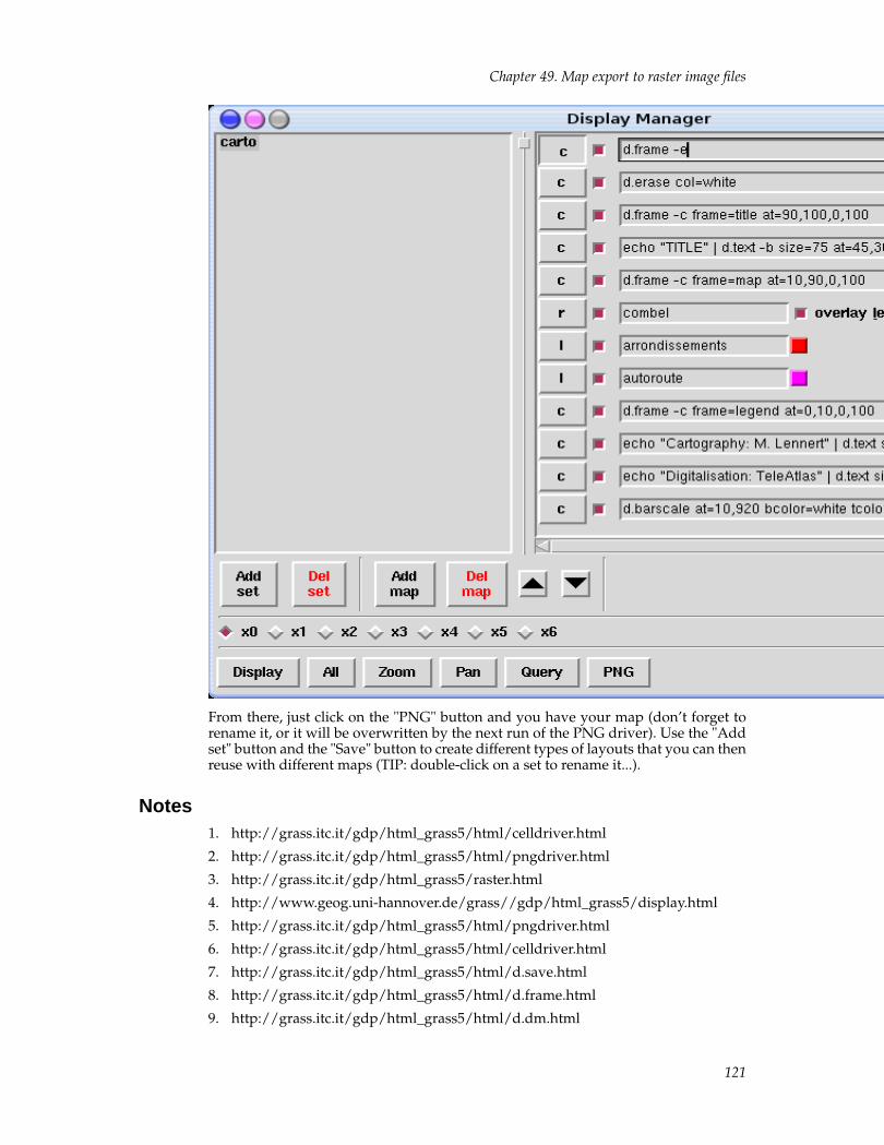
Chapter 49. Map export to raster image files
From there, just click on the "PNG" button and you have your map (don’t forget torename it, or it will be overwritten by the next run of the PNG driver). Use the "Addset" button and the "Save" button to create different types of layouts that you can thenreuse with different maps (TIP: double-click on a set to rename it...).
Notes1. http://grass.itc.it/gdp/html_grass5/html/celldriver.html
2. http://grass.itc.it/gdp/html_grass5/html/pngdriver.html
3. http://grass.itc.it/gdp/html_grass5/raster.html
4. http://www.geog.uni-hannover.de/grass//gdp/html_grass5/display.html
5. http://grass.itc.it/gdp/html_grass5/html/pngdriver.html
6. http://grass.itc.it/gdp/html_grass5/html/celldriver.html
7. http://grass.itc.it/gdp/html_grass5/html/d.save.html
8. http://grass.itc.it/gdp/html_grass5/html/d.frame.html
9. http://grass.itc.it/gdp/html_grass5/html/d.dm.html
121

Chapter 49. Map export to raster image files
122
Chapter 50. Postscript Maps/Exports
The ps.map1 module offers the possibility to create very fine-tuned maps inpostscript. Next to some interesting options that do not exist as display commandsin GRASS, the great advantage over the raster export drivers is the fact that thepostscript format can be transformed into a vector format which allows reworkingparts of the file in vector graphics programs (see the Section called Editing theresulting postscript file with pstoedit for more details).
For beginners, the possibility of interactive usage of ps.map is very helpful, but manyof its options are not available interactively and it is, therefore, recommended to cre-ate a script file with the instructions, once you are familiar with the general concept.
Interactive usage
For newcomers to ps.map, this is the best way to begin to learn the usage of ps.map.Just answer the questions, and be sure, at the end, to answer "y" to the question "doyou want to save the script file? (y/n)". This will allow you to look at a script file inorder to learn from it and adapt it for more fine-grained control (see next subsection).In order to visualize your map, use the postscript viewer of your system (ghostview,gv, etc...).
Scripted usage
This is where the entire power of ps.map really comes to play. Just have a look atall the commands listed on the manual page2 and you will get an idea of the possi-bilities offered. Having to write commands into a script file might seem a bit scaryto some and definitely seems a bit outdated in our times of "point the mouse andlet the computer do the rest for you", but once you understand the basic principlesof ps.map, and once you have one or two finished script files at hand (created, forexample, through interactive usage of ps.map), you will soon feel the convenience ofjust typing a few commands to create a very decent layout for your maps. This is alsovery practical when you work in a team as you can create one template script whichwill create the same layout for everyone and in which each team member only has toadd a few commands to draw her maps.
All the commands are listed and explained on the manual page3, so we won’t coverthose here. Be sure to look at the example script at the end of that page. However,here are some tips that might help you:
• One frequent source of error is the omission of an end statement at the end of acommand block. Always include these, as they also help you make your scriptmore readable.
• In the same line, use comments in your file to explain what you are doing (com-ments are anything written after a "#" character) and use line spaces to make itreadable.
• In general, you can trust ps.map to place items correctly, so only use the "where="if you are not satisfied with the automatic placements.
• If you use the colortable command on a raster file with many different values, trythe "cols" option in order to get all your classes onto the map.
• As one of the hidden treasures of GRASS, there is a ps.map.barscale module thatcreates a GRASS vector file and a ps.map script file for a barscale. Just launch thecommand, answer the questions and include the resulting script file into your gen-eral ps.map script file (possibly with the read command).
Generally, all you have to do once you have a script ready, is launch ps.map as fol-lows:
123
Chapter 50. Postscript Maps/Exports
ps.map in=NameOfYourScriptFile out=NameOfThePSFile
Easy, isn’t it ? ;-)
Editing the resulting postscript file with pstoedit
The file containing your finished map after running ps.map is in postscript, the uni-versal printing command language. There are not many programs that allow youto edit a postscript file directly (well, actually there are: text editors, but unless youare willing to learn the entire postscript command language, this won’t be of muchhelp to you). So, you can normally use your postscript file only in the same way youwould a raster graphics file (i.e. .png or .jpeg), meaning that you cannot edit individ-ual objects of the map, only each individual pixel.
However, there is a very handy little free software tool called pstoedit4, written byWolfgang Glunz. This allows you to transform your postscript file into a host of dif-ferent vector formats which you can then edit easily in the relevant vector graphicsprogram. For example, in order to translate a postscript file into a skencil5 (formerly"sketch") file, just type:
pstoedit -f sk YourPostscriptFile.ps ResultingFileName.sk
Then you can edit the entire map, including individual areas, lines and points in theskencil program.
Notes1. http://grass.itc.it/gdp/html_grass5/html/ps.map.html
2. http://grass.itc.it/gdp/html_grass5/html/ps.map.html
3. http://grass.itc.it/gdp/html_grass5/html/ps.map.html
4. http://www.pstoedit.net/pstoedit/
5. http://sketch.sourceforge.net/
124

Chapter 51. HTML Maps/Exports
125

Chapter 51. HTML Maps/Exports
126
Chapter 52. Using external programs for map layout
Since GRASS is specialized in geographical information management and not ingraphical layout, it is often necessary to rework the resulting maps in a real graphicsprogram. Several such programs exist in the free software world, and you will justhave to choose the one you prefer personally. We can divide them into those thatuse formats that you can transform your postscript file into (using pstoedit1 - see theSection called Editing the resulting postscript file with pstoedit in Chapter 50), thereforeallowing direct editing, and those that can only import non-editable raster files (e.g.PNG):
Editable vector import
• Skencil2
• XFig3
• Other suggestions ?
Non-editable raster import
• OpenOffice Draw4
• Tgif5
• Other suggestions ?
Notes1. http://www.pstoedit.net/pstoedit
2. http://sketch.sourceforge.net/
3. http://www.xfig.org/
4. http://www.openoffice.org/product/draw.html
5. http://bourbon.usc.edu:8001/tgif/index.html
127

Chapter 52. Using external programs for map layout
128
Chapter 53. Scripting GRASS
Scripts
The possibility to automate individual steps is a very useful extension (even forGRASS beginners). These scripts have to be written in ASCII format as UNIX shellscripts. Within those scripts GRASS modules can be called with their respective pa-rameters and geostatistical computations can be done automatically. Especially fornovices it is a good idea to generate scripts step by step, trying the commands oncommand line in the terminal first. Later the UNIX command \texttt{\$~history} al-lows viewing and saving ("copy" - "paste" into a text editor with left and middlemouse button) the previously entered commands.
Here1 is an example that shall demonstrate the potential of script programmingclearly: with this script you can calculate general geostatistical information forraster images2. Save this script as, for example, statistics.sh and set the UNIXpermissions with chmod u+x statistics.sh.
This script can be used after launching GRASS, specify the name of the raster mapto be analyzed as parameter. A modified version of above script exists in GRASS 5under the name of r.univar. In here the output of the GRASS module r.stats4 is trans-ferred to the UNIX program awk by UNIX piping (represented by the ’|’ character).The calculations are done within awk, results are printed on the screen.
The best way to understand GRASS scripting is definitely by studying the manyexisting examples. Just go to the scripts directory if your GRASS implementationand study some of them:
cd $GISBASE/scripts/
A few GRASS modules will help you in your scripts. Those are:
• g.ask5 for comfortable querying the user for map names from the GRASS database
• g.findfile6 to directly find a file in the GRASS database and process it
• g.gisenv7 to query for the settings of some of the GRASS environment variable suchas GISDBASE, LOCATION and MAPSET.
Study their use in the existing GRASS scripts to understand how they work.
For more information on general shell programming please consult the man pageof your shell (on GNU/Linux this is generally the bash shell, so type man bash orfollow on of the many links listed on the Programming Texts and Tutorials8 page.
Batch usage of GRASS
GRASS can be completely controlled externally through scripts (and therefore runautomatically) by setting the correct environment variables. There doesn’t exist a sin-gle "GRASS" program, in fact GRASS is a collection of modules which are run in aspecial environment. Even the GRASS startup is simply setting numerous variables.This can be done directly as well, here9 an example in "bash-shell" style.
After having run this script, all GRASS modules that can be used non-interactivelycan be used. Generally, you can get the list of parameters required by a module bytyping "-help" as such a parameter or (always recommended) by reading the manual.
Once these variables have been set, GRASS can also be integrated into CGI, PERLand other scripts. You can visit a quite complex example on the internet: SlideLinks10
which is an online GIS based completely on CGI scripts, a database managementsystem and GRASS.
Since GRASS 5.0 you can alternatively skip the startup screen by directly specifyingthe database, location and mapset:
129
Chapter 53. Scripting GRASS
grass5 /home/neteler/grassdata/katmandu/innercity
Obviously, this only works if the location and the other settings really exist.
Notes1. http://mpa.itc.it/grasstutor/scripts/statistics.sh.txt
2. The code example links in this chapter go to
3. http://mpa.itc.it/grassbook/.
3. http://mpa.itc.it/grassbook/
4. http://grass.itc.it/gdp/html_grass5/html/r.stats.html
5. http://grass.itc.it/gdp/html_grass5/html/g.ask.html
6. http://grass.itc.it/gdp/html_grass5/html/g.findfile.html
7. http://grass.itc.it/gdp/html_grass5/html/g.gisenv.html
8. http://stommel.tamu.edu/~baum/programming.html#shells
9. http://mpa.itc.it/grasstutor/scripts/grass_batch.sh.txt
10. http://gisws.media.osaka-cu.ac.jp/grasslinks/
130
Chapter 54. C-Programming
All important aspects of C programming for GRASS are described in the GRASS 5.0Programmer’s Manual (PDF, 2.3MB)1. This section shall just give an overview howGRASS modules are usually structured. Generally, it will be helpful to look at some ofthe (over 350) existing modules as examples for learning (you can browse the sourcecode via the CVS web interface2). Only an "open source" GIS such as GRASS offersthese deep insights into the "heart" of a GIS. The general structure of the modules isalways similar, each module is stored in a directory of the GRASS source code.
The current source code structure is as follows:3
GRASS GIS library (most relevant only):
html/
modules descriptions
src/CMD/
internal scripts for compilation
src/include/
header files
src/libes/
GIS library routines
src/display/devices/
display driver
src/fonts/
character fonts
src/front.end/
internal routines for the interactive mode of modules
Modules (standard tree):
src/display/
modules for displaying maps on the GRASS monitor
src/general/
file management modules
src/imagery/
image processing modules
src/mapdev/
vector modules
src/misc/
miscellaneous modules
src/paint/
paint driver (PPM)
131
Chapter 54. C-Programming
src/ps.map/
postscript driver
src/raster/
raster modules
src/scripts/
scripts
src/sites/
point modules
src/tcltkgrass/
Tcl/Tk GUI
Other modules:
src.contrib/
contributions of various institutions (however, many are in standard tree as well)
src.garden/
modules with linked simulation models and various interfaces
The existing GRASS modules are built upon the "GRASS programming library"which offers a multitude of GIS functions. It is structured as follows (square bracketscontain the typical function name prefixes for the respective library routines):
GIS library:
database routines (GRASS file management), memory management, parser(string analysis), projections, etc. [G_]
vector library:
management of area, line, and site vectors [Vect_, V2_, dig_]
raster library:
raster data management [R_]
site data library:
site data management [G_sites_]
display library:
graphical output to the monitor [D_]
driver library:
printer driver
image data library:
image processing file management [I_]
segment library:
segmented data management [segment_]
132
Chapter 54. C-Programming
vask library:
control of cursor keys etc. [V_]
rowio library:
for parallel row analysis of raster data [rowio_]
Some of the routines offered are quite substantial. For example they allow calculatinggeodesic distances out of given coordinate points, others perform queries on vectorareas (e.g.: point-in-polygon tests).
Modules consist of the C program files (*.c), the header files (*.h) and a Gmakefile .GRASS has its own "make" routine: gmake5. The file Gmakefile contains instructionsconcerning the files to be compiled and the libraries to be used (GRASS and UNIXlibraries). It has a specific pattern that must be respected. A simple example5 (impor-tant: indents with tab, not with space!) shall demonstrate the typical structure.6
The line "\$(HOME)/\$(PGM)..." and the next contain the compiler instructions,above this section the variables are set. Variables not set here are defined automati-cally in
grass5/src/CMD/head/head.$ARCH
where $ARCH is the name of the system architecture. Starting from GRASS 5.0 this"head" file is created automatically for the used computer platform by the "config-ure" script, which has to be run before the first compilation. The $(HOME) variableindicates where the binary file (i.e. the module) will be copied to: in this example itis the standard path for modules that offer command line support (no limitation tointeractive only usage): grass5/etc/bin/cmd/ .
The actual C program should be divided by (sub-)functionality into several fileswhich have to be listed respectively in the list of objects in the Gmakefile . For de-tails please refer to the "GRASS Programmer’s manual" as this book cannot cover afull C programming tutorial. GRASS GIS library commands can be used directly inthe source code. Interactive parameter querying is made possible by GRASS-specificparameter programming. Here8 is a short example of a raster module.
The calculation is done row and column wise (see "for" loop). As denoted above, it isadvisable to divide the entire module into individual, thematically organized files inorder to facilitate program maintenance.
Notes1. http://grass.itc.it/grass5/progmangrass50.pdf
2. http://freegis.org/cgi-bin/viewcvs.cgi/
3. This will change with new versions of GRASS in an effort to put more commonroutines into libraries and with the integration of a completely new vector engine(see the
4. http://grass.itc.it/grass51/manuals/).
4. http://grass.itc.it/grass51/manuals/
5. http://mpa.itc.it/grasstutor/scripts/code_Gmakefile_pre4
6. The code example links in this chapter go to
7. http://mpa.itc.it/grassbook/.
7. http://mpa.itc.it/grassbook/
8. http://mpa.itc.it/grasstutor/scripts/landsat.c
133

Chapter 54. C-Programming
134

Chapter 55. Digital Terrain Models
GRASS - Geographic Resources Analysis Support System
x
x
x
x
x
x
x
x
x
x
x
x
x
135

Chapter 55. Digital Terrain Models
136
Chapter 56. Topographical analysis
GRASS - Geographic Resources Analysis Support System
x
x
x
x
x
x
x
x
x
x
x
x
x
137

Chapter 56. Topographical analysis
138
Chapter 57. Cost Surfaces
GRASS - Geographic Resources Analysis Support System
x
x
x
x
x
x
x
x
x
x
x
x
x
139

Chapter 57. Cost Surfaces
140
Chapter 58. Creating Animations
GRASS - Geographic Resources Analysis Support System
x
x
x
x
x
x
x
x
x
x
x
x
x
141

Chapter 58. Creating Animations
142
Chapter 59. Bibliography
GRASS - Geographic Resources Analysis Support System1
See GRASS Documentation project2 (Books and tutorials). Major parts of this tutorialhave been translated and updated from the book:
Neteler, M. (2000): GRASS-Handbuch. Der praktische Leitfaden zum Geographis-chen Informationssystem GRASS.3 Geosynthesis 11, Geographisches Institut der Uni-versität Hannover, 247 S. ISBN 3-927053-30-9 (A GRASS beginners tutorial in Germanlanguage)
Search with CiteSeer4 (published GRASS papers).
Notes1. http://grass.itc.it/index.html
2. http://grass.itc.it/gdp/index.html#tutorials
3. http://grass.itc.it/gdp/handbuch/index.html
4. http://citeseer.nj.nec.com/cs?q=grass+gis
143

Chapter 59. Bibliography
144
Appendix A. GNU Free Documentation License
Copyright (C) 2000,2001,2002 Free Software Foundation, Inc. 59 Temple Place, Suite 330,Boston, MA 02111-1307 USA Everyone is permitted to copy and distribute verbatimcopies of this license document, but changing it is not allowed.
PREAMBLE
The purpose of this License is to make a manual, textbook, or other functional anduseful document "free" in the sense of freedom: to assure everyone the effective free-dom to copy and redistribute it, with or without modifying it, either commercially ornoncommercially. Secondarily, this License preserves for the author and publisher away to get credit for their work, while not being considered responsible for modifi-cations made by others.
This License is a kind of "copyleft", which means that derivative works of the docu-ment must themselves be free in the same sense. It complements the GNU GeneralPublic License, which is a copyleft license designed for free software.
We have designed this License in order to use it for manuals for free software, becausefree software needs free documentation: a free program should come with manualsproviding the same freedoms that the software does. But this License is not limitedto software manuals; it can be used for any textual work, regardless of subject matteror whether it is published as a printed book. We recommend this License principallyfor works whose purpose is instruction or reference.
APPLICABILITY AND DEFINITIONS
This License applies to any manual or other work, in any medium, that contains anotice placed by the copyright holder saying it can be distributed under the termsof this License. Such a notice grants a world-wide, royalty-free license, unlimitedin duration, to use that work under the conditions stated herein. The "Document",below, refers to any such manual or work. Any member of the public is a licensee,and is addressed as "you". You accept the license if you copy, modify or distribute thework in a way requiring permission under copyright law.
A "Modified Version" of the Document means any work containing the Document ora portion of it, either copied verbatim, or with modifications and/or translated intoanother language.
A "Secondary Section" is a named appendix or a front-matter simplesect of the Doc-ument that deals exclusively with the relationship of the publishers or authors ofthe Document to the Document’s overall subject (or to related matters) and containsnothing that could fall directly within that overall subject. (Thus, if the Document isin part a textbook of mathematics, a Secondary Section may not explain any mathe-matics.) The relationship could be a matter of historical connection with the subjector with related matters, or of legal, commercial, philosophical, ethical or political po-sition regarding them.
The "Invariant Sections" are certain Secondary Sections whose titles are designated,as being those of Invariant Sections, in the notice that says that the Document isreleased under this License. If a simplesect does not fit the above definition of Sec-ondary then it is not allowed to be designated as Invariant. The Document may con-tain zero Invariant Sections. If the Document does not identify any Invariant Sectionsthen there are none.
The "Cover Texts" are certain short passages of text that are listed, as Front-CoverTexts or Back-Cover Texts, in the notice that says that the Document is released underthis License. A Front-Cover Text may be at most 5 words, and a Back-Cover Text maybe at most 25 words.
145
Appendix A. GNU Free Documentation License
A "Transparent" copy of the Document means a machine-readable copy, representedin a format whose specification is available to the general public, that is suitablefor revising the document straightforwardly with generic text editors or (for imagescomposed of pixels) generic paint programs or (for drawings) some widely availabledrawing editor, and that is suitable for input to text formatters or for automatic trans-lation to a variety of formats suitable for input to text formatters. A copy made in anotherwise Transparent file format whose markup, or absence of markup, has beenarranged to thwart or discourage subsequent modification by readers is not Trans-parent. An image format is not Transparent if used for any substantial amount oftext. A copy that is not "Transparent" is called "Opaque".
Examples of suitable formats for Transparent copies include plain ASCII withoutmarkup, Texinfo input format, LaTeX input format, SGML or XML using a publiclyavailable DTD, and standard-conforming simple HTML, PostScript or PDF designedfor human modification. Examples of transparent image formats include PNG, XCFand JPG. Opaque formats include proprietary formats that can be read and editedonly by proprietary word processors, SGML or XML for which the DTD and/orprocessing tools are not generally available, and the machine-generated HTML,PostScript or PDF produced by some word processors for output purposes only.
The "Title Page" means, for a printed book, the title page itself, plus such followingpages as are needed to hold, legibly, the material this License requires to appear in thetitle page. For works in formats which do not have any title page as such, "Title Page"means the text near the most prominent appearance of the work’s title, preceding thebeginning of the body of the text.
A simplesect "Entitled XYZ" means a named subunit of the Document whose titleeither is precisely XYZ or contains XYZ in parentheses following text that translatesXYZ in another language. (Here XYZ stands for a specific simplesect name mentionedbelow, such as "Acknowledgements", "Dedications", "Endorsements", or "History".)To "Preserve the Title" of such a simplesect when you modify the Document meansthat it remains a simplesect "Entitled XYZ" according to this definition.
The Document may include Warranty Disclaimers next to the notice which states thatthis License applies to the Document. These Warranty Disclaimers are considered tobe included by reference in this License, but only as regards disclaiming warranties:any other implication that these Warranty Disclaimers may have is void and has noeffect on the meaning of this License.
VERBATIM COPYING
You may copy and distribute the Document in any medium, either commercially ornoncommercially, provided that this License, the copyright notices, and the licensenotice saying this License applies to the Document are reproduced in all copies, andthat you add no other conditions whatsoever to those of this License. You may notuse technical measures to obstruct or control the reading or further copying of thecopies you make or distribute. However, you may accept compensation in exchangefor copies. If you distribute a large enough number of copies you must also followthe conditions in simplesect 3.
You may also lend copies, under the same conditions stated above, and you maypublicly display copies.
COPYING IN QUANTITY
If you publish printed copies (or copies in media that commonly have printed cov-ers) of the Document, numbering more than 100, and the Document’s license noticerequires Cover Texts, you must enclose the copies in covers that carry, clearly andlegibly, all these Cover Texts: Front-Cover Texts on the front cover, and Back-CoverTexts on the back cover. Both covers must also clearly and legibly identify you as thepublisher of these copies. The front cover must present the full title with all words
146
Appendix A. GNU Free Documentation License
of the title equally prominent and visible. You may add other material on the coversin addition. Copying with changes limited to the covers, as long as they preserve thetitle of the Document and satisfy these conditions, can be treated as verbatim copyingin other respects.
If the required texts for either cover are too voluminous to fit legibly, you should putthe first ones listed (as many as fit reasonably) on the actual cover, and continue therest onto adjacent pages.
If you publish or distribute Opaque copies of the Document numbering more than100, you must either include a machine-readable Transparent copy along with eachOpaque copy, or state in or with each Opaque copy a computer-network locationfrom which the general network-using public has access to download using public-standard network protocols a complete Transparent copy of the Document, free ofadded material. If you use the latter option, you must take reasonably prudent steps,when you begin distribution of Opaque copies in quantity, to ensure that this Trans-parent copy will remain thus accessible at the stated location until at least one yearafter the last time you distribute an Opaque copy (directly or through your agents orretailers) of that edition to the public.
It is requested, but not required, that you contact the authors of the Document wellbefore redistributing any large number of copies, to give them a chance to provideyou with an updated version of the Document.
MODIFICATIONS
You may copy and distribute a Modified Version of the Document under the condi-tions of simplesects 2 and 3 above, provided that you release the Modified Versionunder precisely this License, with the Modified Version filling the role of the Docu-ment, thus licensing distribution and modification of the Modified Version to who-ever possesses a copy of it. In addition, you must do these things in the ModifiedVersion:
A. Use in the Title Page (and on the covers, if any) a title distinct from that of theDocument, and from those of previous versions (which should, if there wereany, be listed in the History simplesect of the Document). You may use thesame title as a previous version if the original publisher of that version givespermission.
B. List on the Title Page, as authors, one or more persons or entities responsiblefor authorship of the modifications in the Modified Version, together with atleast five of the principal authors of the Document (all of its principal authors,if it has fewer than five), unless they release you from this requirement.
C. State on the Title page the name of the publisher of the Modified Version, asthe publisher.
D. Preserve all the copyright notices of the Document.
E. Add an appropriate copyright notice for your modifications adjacent to theother copyright notices.
F. Include, immediately after the copyright notices, a license notice giving thepublic permission to use the Modified Version under the terms of this License,in the form shown in the Addendum below.
G. Preserve in that license notice the full lists of Invariant Sections and requiredCover Texts given in the Document’s license notice.
H. Include an unaltered copy of this License.
I. Preserve the simplesect Entitled "History", Preserve its Title, and add to it anitem stating at least the title, year, new authors, and publisher of the ModifiedVersion as given on the Title Page. If there is no simplesect Entitled "History"
147
Appendix A. GNU Free Documentation License
in the Document, create one stating the title, year, authors, and publisher of theDocument as given on its Title Page, then add an item describing the ModifiedVersion as stated in the previous sentence.
J. Preserve the network location, if any, given in the Document for public ac-cess to a Transparent copy of the Document, and likewise the network loca-tions given in the Document for previous versions it was based on. These maybe placed in the "History" simplesect. You may omit a network location for awork that was published at least four years before the Document itself, or ifthe original publisher of the version it refers to gives permission.
K. For any simplesect Entitled "Acknowledgements" or "Dedications", Preservethe Title of the simplesect, and preserve in the simplesect all the substance andtone of each of the contributor acknowledgements and/or dedications giventherein.
L. Preserve all the Invariant Sections of the Document, unaltered in their text andin their titles. Section numbers or the equivalent are not considered part of thesimplesect titles.
M. Delete any simplesect Entitled "Endorsements". Such a simplesect may not beincluded in the Modified Version.
N. Do not retitle any existing simplesect to be Entitled "Endorsements" or to con-flict in title with any Invariant Section.
O. Preserve any Warranty Disclaimers.
If the Modified Version includes new front-matter simplesects or appendices thatqualify as Secondary Sections and contain no material copied from the Document,you may at your option designate some or all of these simplesects as invariant. To dothis, add their titles to the list of Invariant Sections in the Modified Version’s licensenotice. These titles must be distinct from any other simplesect titles.
You may add a simplesect Entitled "Endorsements", provided it contains nothing butendorsements of your Modified Version by various parties--for example, statementsof peer review or that the text has been approved by an organization as the authori-tative definition of a standard.
You may add a passage of up to five words as a Front-Cover Text, and a passageof up to 25 words as a Back-Cover Text, to the end of the list of Cover Texts in theModified Version. Only one passage of Front-Cover Text and one of Back-Cover Textmay be added by (or through arrangements made by) any one entity. If the Docu-ment already includes a cover text for the same cover, previously added by you or byarrangement made by the same entity you are acting on behalf of, you may not addanother; but you may replace the old one, on explicit permission from the previouspublisher that added the old one.
The author(s) and publisher(s) of the Document do not by this License give permis-sion to use their names for publicity for or to assert or imply endorsement of anyModified Version.
COMBINING DOCUMENTS
You may combine the Document with other documents released under this License,under the terms defined in simplesect 4 above for modified versions, provided thatyou include in the combination all of the Invariant Sections of all of the original doc-uments, unmodified, and list them all as Invariant Sections of your combined workin its license notice, and that you preserve all their Warranty Disclaimers.
The combined work need only contain one copy of this License, and multiple identi-cal Invariant Sections may be replaced with a single copy. If there are multiple Invari-ant Sections with the same name but different contents, make the title of each suchsimplesect unique by adding at the end of it, in parentheses, the name of the originalauthor or publisher of that simplesect if known, or else a unique number. Make the
148
Appendix A. GNU Free Documentation License
same adjustment to the simplesect titles in the list of Invariant Sections in the licensenotice of the combined work.
In the combination, you must combine any simplesects Entitled "History" in the vari-ous original documents, forming one simplesect Entitled "History"; likewise combineany simplesects Entitled "Acknowledgements", and any simplesects Entitled "Dedi-cations". You must delete all simplesects Entitled "Endorsements".
COLLECTIONS OF DOCUMENTS
You may make a collection consisting of the Document and other documents releasedunder this License, and replace the individual copies of this License in the variousdocuments with a single copy that is included in the collection, provided that youfollow the rules of this License for verbatim copying of each of the documents in allother respects.
You may extract a single document from such a collection, and distribute it individu-ally under this License, provided you insert a copy of this License into the extracteddocument, and follow this License in all other respects regarding verbatim copyingof that document.
AGGREGATION WITH INDEPENDENT WORKS
A compilation of the Document or its derivatives with other separate and indepen-dent documents or works, in or on a volume of a storage or distribution medium, iscalled an "aggregate" if the copyright resulting from the compilation is not used tolimit the legal rights of the compilation’s users beyond what the individual workspermit. When the Document is included in an aggregate, this License does not applyto the other works in the aggregate which are not themselves derivative works of theDocument.
If the Cover Text requirement of simplesect 3 is applicable to these copies of the Doc-ument, then if the Document is less than one half of the entire aggregate, the Docu-ment’s Cover Texts may be placed on covers that bracket the Document within theaggregate, or the electronic equivalent of covers if the Document is in electronic form.Otherwise they must appear on printed covers that bracket the whole aggregate.
TRANSLATION
Translation is considered a kind of modification, so you may distribute translationsof the Document under the terms of simplesect 4. Replacing Invariant Sections withtranslations requires special permission from their copyright holders, but you mayinclude translations of some or all Invariant Sections in addition to the original ver-sions of these Invariant Sections. You may include a translation of this License, andall the license notices in the Document, and any Warranty Disclaimers, provided thatyou also include the original English version of this License and the original versionsof those notices and disclaimers. In case of a disagreement between the translationand the original version of this License or a notice or disclaimer, the original versionwill prevail.
If a simplesect in the Document is Entitled "Acknowledgements", "Dedications", or"History", the requirement (simplesect 4) to Preserve its Title (simplesect 1) will typi-cally require changing the actual title.
TERMINATION
You may not copy, modify, sublicense, or distribute the Document except as expresslyprovided for under this License. Any other attempt to copy, modify, sublicense or
149
Appendix A. GNU Free Documentation License
distribute the Document is void, and will automatically terminate your rights underthis License. However, parties who have received copies, or rights, from you underthis License will not have their licenses terminated so long as such parties remain infull compliance.
FUTURE REVISIONS OF THIS LICENSE
The Free Software Foundation may publish new, revised versions of the GNU FreeDocumentation License from time to time. Such new versions will be similar in spiritto the present version, but may differ in detail to address new problems or concerns.See http://www.gnu.org/copyleft/.
Each version of the License is given a distinguishing version number. If the Docu-ment specifies that a particular numbered version of this License "or any later ver-sion" applies to it, you have the option of following the terms and conditions eitherof that specified version or of any later version that has been published (not as adraft) by the Free Software Foundation. If the Document does not specify a versionnumber of this License, you may choose any version ever published (not as a draft)by the Free Software Foundation.
ADDENDUM: How to use this License for your documents
To use this License in a document you have written, include a copy of the License inthe document and put the following copyright and license notices just after the titlepage:
Copyright (c) YEAR YOUR NAME. Permission is granted to copy, distribute and/ormodify this document under the terms of the GNU Free Documentation License, Version1.2 or any later version published by the Free Software Foundation; with no Invariant Sec-tions, no Front-Cover Texts, and no Back-Cover Texts. A copy of the license is included inthe simplesect entitled "GNU Free Documentation License".
If you have Invariant Sections, Front-Cover Texts and Back-Cover Texts, replace the"with...Texts." line with this:
with the Invariant Sections being LIST THEIR TITLES, with the Front-Cover Texts beingLIST, and with the Back-Cover Texts being LIST.
If you have Invariant Sections without Cover Texts, or some other combination of thethree, merge those two alternatives to suit the situation.
If your document contains nontrivial examples of program code, we recommend re-leasing these examples in parallel under your choice of free software license, such asthe GNU General Public License, to permit their use in free software.
150