batch mode reinforcement learning based on the …ernst/uploads/news/id144/fonteneau2013...batch...
TRANSCRIPT

Ann Oper ResDOI 10.1007/s10479-012-1248-5
Batch mode reinforcement learning basedon the synthesis of artificial trajectories
Raphael Fonteneau · Susan A. Murphy ·Louis Wehenkel · Damien Ernst
© Springer Science+Business Media New York 2012
Abstract In this paper, we consider the batch mode reinforcement learning setting, wherethe central problem is to learn from a sample of trajectories a policy that satisfies or opti-mizes a performance criterion. We focus on the continuous state space case for which usualresolution schemes rely on function approximators either to represent the underlying controlproblem or to represent its value function. As an alternative to the use of function approxima-tors, we rely on the synthesis of “artificial trajectories” from the given sample of trajectories,and show that this idea opens new avenues for designing and analyzing algorithms for batchmode reinforcement learning.
Keywords Reinforcement learning · Optimal control · Artificial trajectories · Functionapproximators
1 Introduction
Optimal control problems arise in many real-life applications, such as engineering (Ried-miller 2005), medicine (Robins 1986; Murphy et al. 2001; Murphy 2003) or artificial in-telligence (Sutton and Barto 1998). Over the last decade, techniques developed by the Re-inforcement Learning (RL) community (Sutton and Barto 1998) have become more andmore popular for addressing those types of problems. RL was initially focusing on how to
R. Fonteneau (�) · L. Wehenkel · D. ErnstUniversity of Liège, Liège, Belgiume-mail: [email protected]
L. Wehenkele-mail: [email protected]
D. Ernste-mail: [email protected]
S.A. MurphyUniversity of Michigan, Ann Arbor, USAe-mail: [email protected]

Ann Oper Res
design intelligent agents able to interact with their environment so as to optimize a given per-formance criterion (Sutton and Barto 1998). Since the end of the nineties, many researchershave focused on the resolution of a subproblem of RL: computing high performance policieswhen the only information available on the environment is contained in a batch collectionof trajectories. This subproblem of RL is referred to as batch mode RL (Fonteneau 2011).
Most of the techniques proposed in the literature for solving batch mode RL problemsover large or continuous spaces combine value or policy iteration schemes from the Dy-namic Programming (DP) theory (Bellman 1957) with function approximators (e.g., radialbasis functions, neural networks, etc.) representing (state-action) value functions (Busoniuet al. 2010). These approximators have two main roles: (i) to offer a concise representa-tion of state-action value functions defined over continuous spaces and (ii) to generalizethe information contained in the finite sample of input data. Another family of algorithmsthat has been less studied in RL adopts a two stage process for solving these batch modeRL problems. First, they train function approximators to learn a model of the environmentand, afterwards, they use various optimization schemes (e.g., direct policy search, dynamicprogramming) to compute a policy which is (near-)optimal with respect to this model.
While successful in many studies, the use of function approximators for solving batchmode RL problems has also drawbacks. In particular, the black box nature of this approachmakes performance analysis very difficult, and hence severely hinders the design of newbatch mode RL algorithms presenting some a priori desired performance guarantees. Also,the policies inferred by these algorithms may have counter-intuitive properties. For example,in a deterministic framework, for a fixed initial state, and when there is in the input samplea trajectory that has been generated by an optimal policy starting from this initial state,there is no guarantee that a function approximator-based policy will reproduce this optimalbehavior. This is surprising, since a simple “imitative learning” approach would have such adesirable property.
The above observations have lead us to develop a new line of research based on thesynthesis of “artificial trajectories” for addressing batch mode RL problems. In our ap-proach, artificial trajectories are rebuilt from the tuples extracted from the given batchof trajectories with the aim of achieving an optimality property. In this paper, we re-visit our work on this topic Fonteneau et al. (2009, 2010a, 2010b, 2010c, 2010d), withthe objective of showing that these ideas open avenues for addressing many batch modeRL related problems. In particular, four algorithms that exploit artificial trajectories willbe presented. The first one computes an estimate of the performance of a given controlpolicy (Fonteneau et al. 2010c). The second one provides a way for computing perfor-mance guarantees in deterministic settings (Fonteneau et al. 2009). The third one leads tothe computation of policies having high performance guarantees (Fonteneau et al. 2010a;Fonteneau et al. 2010d), and the fourth algorithm presents a sampling strategy for gen-erating additional trajectories (Fonteneau et al. 2010b). Finally, we highlight connectionsbetween the concept of artificial trajectory synthesis and other standard batch mode RLtechniques.
The paper is organized as follows. First, Sect. 2 gives a brief review of the field of batchmode RL. Section 3 presents the batch mode RL setting adopted in this paper and severalof the generic problems it raises. In Sect. 4, we present our new line of research articu-lated around the synthesis of artificial trajectories. Finally, Sect. 5 proposes to make the linkbetween this paradigm and existing batch mode RL techniques, and Sect. 6 concludes.

Ann Oper Res
2 Related work
Batch mode RL techniques are probably rooted in the works of Bradtke and Barto (1996) andBoyan (2005) related to the use of least-squares techniques in the context of Temporal Dif-ference learning methods (LSTD) for estimating the return of control policies. Those workshave been extended to address optimal control problems by Lagoudakis and Parr (2003) whohave introduced the Least-Square Policy Iteration (LSPI) algorithm that mimics the policyiteration algorithm of the DP theory (Bellman 1957). Several papers have proposed sometheoretical works related to least-squares TD-based algorithms, such as for example Nedicand Bertsekas (2003) and Lazaric et al. (2010a, 2010b).
Another algorithm from the DP theory, the value iteration algorithm, has also servedas inspiration for designing batch mode RL algorithms. For example, Ormoneit and Senhave developed a batch mode RL algorithm in 2002 (Ormoneit and Sen 2002) using kernelapproximators, for which theoretical analyses are also provided. Ernst et al. (2003) proposesan algorithm that combines value iteration with any type of regressors (e.g., regression trees,SVMs, neural networks). Ernst et al. (2005) has named this algorithm Fitted Q Iteration(FQI) and provides a careful empirical analysis of its performance when combined withensembles of regression trees.
Riedmiller (2005), Lange and Riedmiller (2010) and Timmer and Riedmiller (2007)study the performances of this FQI algorithm with (deep) neural networks and CMACs(Cerebella Model Articulator Controllers). The Regularized FQI algorithm proposes to usepenalized least-squares regression as function approximator to limit the model-complexityof the original FQI algorithm (Farahmand et al. 2008). Extensions of the FQI algorithmto continuous action spaces have also been proposed (Antos et al. 2007). More theo-retical works related with FQI have also been published (Munos and Szepesvári 2008;Chakraborty et al. 2008).
Applications of these batch mode RL techniques have already led to promising results inrobotics (Peters et al. 2003; Bonarini et al. 2008; Tognetti et al. 2009), power systems (Ernstet al. 2009), image processing (Ernst et al. 2006a), water reservoir optimization (Castellettiet al. 2007, 2010), medicine (Murphy 2003; Ernst et al. 2006b; Guez et al. 2008) and drivingassistance strategies (Pietquin et al. 2011).
3 Batch mode RL: formalization and typical problems
We consider a stochastic discrete-time system whose dynamics is given by
xt+1 = f (xt , ut ,wt ) ∀t ∈ {0, . . . , T − 1}where xt belongs to a state space X ⊂ R
d , where Rd is the d-dimensional Euclidean space
and T ∈ N\{0} denotes the finite optimization horizon. At every time t ∈ {0, . . . , T −1}, thesystem can be controlled by taking an action ut ∈ U , and is subject to a random disturbancewt ∈ W drawn according to a probability distribution pW (·).1 With each system transitionfrom time t to t + 1 is associated a reward signal:
rt = ρ(xt , ut ,wt ) ∀t ∈ {0, . . . , T − 1}.
1Here the fundamental assumption is that wt is independent of wt−1,wt−2, . . . ,w0 given xt and ut ; tosimplify all notations and derivations, we furthermore impose that the process is time-invariant and does notdepend on the states and actions xt , ut .
Ann Oper Res
Let h : {0, . . . , T − 1} × X → U be a control policy. When starting from a given initial statex0 and following the control policy h, an agent will get a random sum of rewards signalRh(x0,w0, . . . ,wT −1):
Rh(x0,w0, . . . ,wT −1) =T −1∑
t=0
ρ(xt , h(t, xt ),wt
)
with xt+1 = f(xt , h(t, xt ),wt
) ∀t ∈ {0, . . . , T − 1}wt ∼ pW (·).
In RL, the classical performance criterion for evaluating a policy h is its expected T -stagereturn:
Definition 1 (Expected T -stage return)
J h(x0) = E[Rh(x0,w0, . . . ,wT −1)
],
but, when searching for risk-aware policies, it is also of interest to consider a risk-sensitivecriterion:
Definition 2 (Risk-sensitive T -stage return) Let b ∈ R and c ∈ [0,1[.
Jh,(b,c)
RS (x0) ={−∞ if P (Rh(x0,w0, . . . ,wT −1) < b) > c,
J h(x0) otherwise.
The central problem of batch mode RL is to find a good approximation of a policy h∗
that optimizes one such performance criterion, given the fact that the functions f , ρ andpW (·) are unknown, and thus not accessible to simulation. Instead, they are “replaced” bya batch collection of n ∈ N \ {0} elementary pieces of trajectories, defined according to thefollowing process.
Definition 3 (Sample of transitions) Let
Pn = {(xl, ul
)}n
l=1∈ (X × U )n
be a given set of state-action pairs. Consider the ensemble of samples of one-step transitionsof size n that could be generated by complementing each pair (xl, ul) of Pn by drawing foreach l a disturbance signal wl at random from pW (.), and by recording the resulting valuesof ρ(xl, ul,wl) and f (xl, ul,wl). We denote by Fn(Pn,w
1, . . . ,wn) one such “random”set of one-step transitions defined by a random draw of n i.i.d. disturbance signals wl , l =1, . . . , n. We assume that we know one realization of the random set Fn(Pn,w
1, . . . ,wn),that we denote by Fn:
Fn = {(xl, ul, rl, yl
)}n
l=1
where, for all l ∈ {1, . . . , n},∀l ∈ {1, . . . , n}, rl = ρ
(xl, ul,wl
),
yl = f(xl, ul,wl
),
for some realizations of the disturbance process wl ∼ pW (·).

Ann Oper Res
Notice first that the resolution of the central problem of finding a good approximation ofan optimal policy h∗ is very much correlated to the problem of estimating the performanceof a given policy. Indeed, when this latter problem is solved, the search for an optimal policycan in principle be reduced to an optimization problem over the set of candidate policies.We thus will start by addressing the problem of characterizing the performance of a givenpolicy.
It is sometimes desirable to be able to compute policies having good performance guar-antees. Indeed, for many applications, even if it is perhaps not paramount to have a policy h
which is very close to the optimal one, it is however crucial to be able to guarantee that theconsidered policy h leads to high-enough cumulated rewards. The problem of computingsuch policies will also be addressed later in this paper.
In many applications, one has the possibility to move away from a pure batch settingby carrying out a limited number of experiments on the real system in order to enrich theavailable sample of trajectories. We thus also consider the problem of designing strategiesfor generating optimal experiments for batch mode RL.
4 Synthesizing artificial trajectories
We first formalize the concept of artificial trajectories in Sect. 4.1. In Sect. 4.2, we detail,analyze and illustrate on a benchmark how artificial trajectories can be exploited for esti-mating the performances of policies. We focus in Sect. 4.3 on the deterministic case, andwe show how artificial trajectories can be used for computing bounds on the performancesof policies. Afterwards, we exploit these bounds for addressing two different problems: thefirst problem (Sect. 4.4) is to compute policies having good performance guarantees. Thesecond problem (Sect. 4.5) is to design sampling strategies for generating additional systemtransitions.
4.1 Artificial trajectories
Artificial trajectories are made of elementary pieces of trajectories (one-step system transi-tions) taken from the sample Fn. Formally, an artificial trajectory is defined as follows:
Definition 4 (Artificial trajectory) An artificial trajectory is an (ordered) sequence of T
one-step system transitions:
[(xl0 , ul0 , rl0 , yl0
), . . . ,
(xlT −1 , ulT −1 , rlT −1 , ylT −1
)] ∈ F Tn
where
lt ∈ {1, . . . , n}, ∀t ∈ {0, . . . , T − 1}.
We give in Fig. 1 an illustration of one such artificial trajectory.Observe that one can synthesize nT different artificial trajectories from the sample of
transitions Fn. In the rest of this paper, we present various techniques for extracting andexploiting “interesting” subsets of artificial trajectories.

Ann Oper Res
Fig. 1 An example of anartificial trajectory rebuilt from4 one-step system transitionsfrom Fn
4.2 Evaluating the expected return of a policy
A major subproblem of batch mode RL is to evaluate the expected return J h(x0) of a givenpolicy h. Indeed, when such an oracle is available, the search for an optimal policy can be insome sense reduced to an optimization problem over the set of all candidate policies. Whena model of the system dynamics, reward function and disturbances probability distributionis available, Monte Carlo estimation techniques can be run to estimate the performance ofany control policy. But, this is indeed not possible in the batch mode setting. In this section,we detail an approach that estimates the performance of a policy by rebuilding artificialtrajectories so as to mimic the behavior of the Monte Carlo estimator. We assume in thissection (and also in Sect. 4.3) that the action space U is continuous and normed.
4.2.1 Monte Carlo estimation
The Monte Carlo (MC) estimator works in a model-based setting (i.e., in a setting wheref , ρ and pW (.) are known). It estimates J h(x0) by averaging the returns of several (sayp ∈ N \ {0}) trajectories which have been generated by simulating the system from x0 usingthe policy h. More formally, the MC estimator of the expected return of the policy h whenstarting from the initial state x0 writes:
Definition 5 (Monte Carlo estimator)
Mhp(x0) = 1
p
p∑
i=1
T −1∑
t=0
ρ(xi
t , h(t, xi
t
),wi
t
)
with ∀t ∈ {0, . . . , T − 1}, ∀i ∈ {1, . . . , p},wi
t ∼ pW (.),
xi0 = x0,
xit+1 = f
(xi
t , h(t, xi
t
),wi
t
).
The bias and variance of the MC estimator are:

Ann Oper Res
Proposition 1 (Bias and variance of the MC estimator)
Ewi
t ∼pW (.), i=1,...,p, t=0,...,T −1
[M
hp(x0) − J h(x0)
] = 0,
Ewi
t ∼pW (.), i=1,...,p, t=0,...,T −1
[(M
hp(x0) − J h(x0)
)2] = σ 2Rh(x0)
p
where σ 2Rh(x0) denotes the assumed finite variance of Rh(x0,w0, . . . ,wT −1):
σ 2Rh(x0) = Var
w0,...,wT −1∼pW (.)
[Rh(x0,w0, . . . ,wT −1)
]< +∞.
4.2.2 Model-free Monte Carlo estimation
From a sample Fn, our model-free MC (MFMC) estimator works by rebuilding p ∈ N \ {0}artificial trajectories. These artificial trajectories will then serve as proxies of p “actual”trajectories that could be obtained by simulating the policy h on the given control problem.Our estimator averages the cumulated returns over these artificial trajectories to computeits estimate of the expected return J h(x0). The main idea behind our method amounts toselecting the artificial trajectories so as to minimize the discrepancy of these trajectorieswith a classical MC sample that could be obtained by simulating the system with policy h.
To rebuild a sample of p artificial trajectories of length T starting from x0 and similar totrajectories that would be induced by a policy h, our algorithm uses each one-step transitionin Fn at most once; we thus assume that pT ≤ n. The p artificial trajectories of T one-steptransitions are created sequentially. Every artificial trajectory is grown in length by selecting,among the sample of not yet used one-step transitions, a transition whose first two elementsminimize the distance—using a distance metric Δ in X × U —with the couple formed bythe last element of the previously selected transition and the action induced by h at theend of this previous transition. Because (i) all disturbances wl , l = 1, . . . , n are state-actionindependent and i.i.d. according to pW (·) and (ii) we do not re-use one-step transitions, thedisturbances associated with the selected transitions are i.i.d., which provides the MFMCestimator with interesting theoretical properties (see Sect. 4.2.3). Consequently, this alsoensures that the p rebuilt artificial trajectories will be distinct.
A tabular version of the algorithm for building the set of artificial trajectories is given inAlgorithm 1. It returns a set of indices of one-step transitions {lit }i=p, t=T −1
i=1, t=0 from Fn basedon h, x0, the distance metric Δ and the parameter p. Based on this set of indices, we defineour MFMC estimate of the expected return of the policy h when starting from the initialstate x0:
Definition 6 (Model-free Monte Carlo estimator)
Mhp(Fn, x0) = 1
p
p∑
i=1
T −1∑
t=0
rlit .
Figure 2 illustrates the MFMC estimator. Note that the computation of the MFMC es-timator Mh
p(Fn, x0) has a linear complexity with respect to the cardinality n of Fn, thenumber of artificial trajectories p and the optimization horizon T .

Ann Oper Res
Algorithm 1 MFMC algorithm to rebuild a set of size p of T -length artificial trajectoriesfrom a sample of n one-step transitions
Input: Fn, h(., .), x0, Δ(., .), T , p
Let G denote the current set of not yet used one-step transitions in Fn; Initially,G ← Fn;for i = 1 to p (extract an artificial trajectory) do
t ← 0;xi
t ← x0;while t < T do
uit ← h(t, xi
t );H ← arg min
(x,u,r,y)∈GΔ((x,u), (xi
t , uit ));
lit ← lowest index in Fn of the transitions that belong to H;t ← t + 1;xi
t ← ylit ;
G ← G \ {(xlit , ulit , r lit , ylit )}; \\ do not re-use transitionsend while
end forReturn the set of indices {lit }i=p, t=T −1
i=1, t=0 .
Fig. 2 Rebuilding three 4-lengthtrajectories for estimating thereturn of a policy
4.2.3 Analysis of the MFMC estimator
In this section we characterize some main properties of our estimator. To this end, we studythe distribution of our estimator Mh
p(Fn(Pn,w1, . . . ,wn), x0), seen as a function of the ran-
dom set Fn(Pn,w1, . . . ,wn); in order to characterize this distribution, we express its bias
and its variance as a function of a measure of the density of the sample Pn, defined by its “k-dispersion”; this is the smallest radius such that all Δ-balls in X × U of this radius containat least k elements from Pn. The use of this notion implies that the space X × U is bounded(when measured using the distance metric Δ).
The bias and variance characterization will be done under some additional assumptionsdetailed below. After that, we state the main theorems formulating these characterizations.Proofs are given in Fonteneau et al. (2010c).

Ann Oper Res
Assumption (Lipschitz continuity of the functions f , ρ and h) We assume that the dynam-ics f , the reward function ρ and the policy h are Lipschitz continuous, i.e., we assume thatthere exist finite constants Lf , Lρ and Lh ∈ R
+ such that: ∀(x, x ′, u,u′,w) ∈ X 2 × U 2 × W ,
∥∥f (x,u,w) − f(x ′, u′,w
)∥∥X ≤ Lf
(∥∥x − x ′∥∥X + ∥∥u − u′∥∥
U
),
∣∣ρ(x,u,w) − ρ(x ′, u′,w
)∣∣ ≤ Lρ
(∥∥x − x ′∥∥X + ∥∥u − u′∥∥
U
),
∥∥h(t, x) − h(t, x ′)∥∥
U ≤ Lh
∥∥x − x ′∥∥X , ∀t ∈ {0, . . . , T − 1},
where ‖.‖X and ‖.‖U denote the chosen norms over the spaces X and U , respectively.
Assumption (X × U is bounded) We suppose that X × U is bounded when measured usingthe distance metric Δ.
Definition 7 (Distance metric Δ)
∀(x, x ′, u,u′) ∈ X 2 × U 2, Δ
((x,u),
(x ′, u′)) = ∥∥x − x ′∥∥
X + ∥∥u − u′∥∥U .
Given k ∈ N \ {0} with k ≤ n, we define the k-dispersion, αk(Pn) of the sample Pn:
Definition 8 (k-dispersion)
αk(Pn) = sup(x,u)∈X ×U
ΔPn
k (x,u),
where ΔPn
k (x,u) denotes the distance of (x,u) to its k-th nearest neighbor (using the dis-tance metric Δ) in the Pn sample. The k-dispersion is the smallest radius such that all Δ-balls in X × U of this radius contain at least k elements from Pn; it can be interpreted asa worst-case measure on how closely Pn covers the X × U space using the k-th nearestneighbors.
Definition 9 (Expected value of Mhp(Fn(Pn,w
1, . . . ,wn), x0)) We denote by Ehp,Pn
(x0) theexpected value:
Ehp,Pn
(x0) = Ew1,...,wn∼pW (.)
[M
hp
(Fn
(Pn,w
1, . . . ,wn), x0
)].
We have the following theorem:
Theorem 1 (Bias bound for Mhp(Fn(Pn,w
1, . . . ,wn), x0))
∣∣J h(x0) − Ehp,Pn
(x0)∣∣ ≤ CαpT (Pn)
with C = Lρ
T −1∑
t=0
T −t−1∑
i=0
(Lf (1 + Lh)
)i.
The proof of this result is given in Fonteneau et al. (2010c). This formula shows that thebias is bounded closer to the target estimate if the sample dispersion is small. Note that thesample dispersion itself actually only depends on the sample Pn and on the value of p (itwill increase with the number of trajectories used by our algorithm).

Ann Oper Res
Definition 10 (Variance of Mhp(Fn(Pn,w
1, . . . ,wn), x0)) We denote by V hp,Pn
(x0) the vari-ance of the MFMC estimator defined by
V hp,Pn
(x0) = Ew1,...,wn∼pW (.)
[(M
hp
(Fn
(Pn,w
1, . . . ,wn), x0
) − Ehp,Pn
(x0))2]
and we give the following theorem:
Theorem 2 (Variance bound for Mhp(Fn(Pn,w
1, . . . ,wn), x0))
V hp,Pn
(x0) ≤(
σRh(x0)√p
+ 2CαpT (Pn)
)2
with C = Lρ
T −1∑
t=0
T −t−1∑
i=0
(Lf (1 + Lh)
)i.
The proof of this theorem is given in Fonteneau et al. (2010c). We see that the varianceof our MFMC estimator is guaranteed to be close to that of the classical MC estimator if thesample dispersion is small enough.
• Illustration. In this section, we illustrate the MFMC estimator on an academic problem.The system dynamics and the reward function are given by
xt+1 = sin
(π
2(xt + ut + wt)
)
and
ρ(xt , ut ,wt ) = 1
2πe− 1
2 (x2t +u2
t ) + wt
with the state space X being equal to [−1,1] and the action space U to [−1,1]. Thedisturbance wt is an element of the interval W = [− ε
2 , ε2 ] with ε = 0.1 and pW is a
uniform probability distribution over this interval. The optimization horizon T is equalto 15. The policy h whose performances have to be evaluated is
h(t, x) = −x
2, ∀x ∈ X , ∀t ∈ {0, . . . , T − 1}.
The initial state of the system is set at x0 = −0.5.
For our first set of experiments, we choose to work with a value of p = 10 i.e., the MFMCestimator rebuilds 10 artificial trajectories to estimate J h(−0.5). In these experiments, fordifferent cardinalities nj = (10j)2 = m2
j , j = 1, . . . ,10, we build a sample Pnj= {(xl, ul)}
that uniformly cover the space X × U as follows:
xl = −1 + 2j1
mj
and ul = −1 + 2j2
mj
, j1, j2 ∈ {0, . . . ,mj − 1}.
Then, we generate 50 random sets F 1nj
, . . . , F 50nj
over Pnjand run our MFMC estimator on
each of these sets. The results of this first set of experiments are gathered in Fig. 3. For everyvalue of nj considered in our experiments, the 50 values computed by the MFMC estima-tor are concisely represented by a boxplot. The box has lines at the lower quartile, median,and upper quartile values. Whiskers extend from each end of the box to the adjacent val-ues in the data within 1.5 times the interquartile range from the ends of the box. Outliersare data with values beyond the ends of the whiskers and are displayed with a red + sign.

Ann Oper Res
Fig. 3 Computations of theMFMC estimator with p = 10,for different cardinalities n of thesample of one-step transitions.For each cardinality, 50independent samples oftransitions have generated.Squares represent Jh(x0)
Fig. 4 Computations of the MCestimator with p = 10. 50independent runs have beencomputed
The squares represent an accurate estimate of J h(−0.5) computed by running thousands ofMonte Carlo simulations. As we observe, when the samples increase in size (which corre-sponds to a decrease of the pT -dispersion αpT (Pn)) the MFMC estimator is more likelyto output accurate estimations of J h(−0.5). As explained throughout this paper, there existmany similarities between the model-free MFMC estimator and the model-based MC esti-mator. These can be empirically illustrated by putting Fig. 3 in perspective with Fig. 4. Thislatter figure reports the results obtained by 50 independent runs of the MC estimator, eachone of these runs using also p = 10 trajectories. As expected, one can see that the MFMCestimator tends to behave similarly to the MC estimator when the cardinality of the sampleincreases.
In our second set of experiments, we choose to study the influence of the number ofartificial trajectories p upon which the MFMC estimator bases its prediction. For each valuepj = j 2, j = 1, . . . ,10 we generate 50 samples F 1
10,000, . . . , F 5010,000 of one-step transitions

Ann Oper Res
Fig. 5 Computations of theMFMC estimator for differentvalues of the number p ofartificial trajectories extractedfrom a sample of n = 10,000tuples. For each value of p, 50independent samples oftransitions have generated.Squares represent Jh(x0)
Fig. 6 Computations of the MCestimator for different values ofthe number of trajectories p. Foreach value of p, 50 independentruns of the MC estimator havebeen computed. Squaresrepresent Jh(x0)
of cardinality 10,000 (using the sample P10,000 defined in the first set of experiments) anduse these samples to compute the MFMC estimator. The results are plotted in Fig. 5. Thisfigure shows that the bias of the MFMC estimator seems to be relatively small for smallvalues of p and to increase with p. This is in accordance with Theorem 1 which bounds thebias with an expression that is increasing with p.
In Fig. 6, we have plotted the evolution of the values computed by the model-based MCestimator when the number of trajectories it considers in its prediction increases. While, forsmall numbers of trajectories, it behaves similarly to the MFMC estimator, the quality of itspredictions steadily improves with p, while it is not the case for the MFMC estimator whoseperformances degrade once p crosses a threshold value. Notice that this threshold valuecould be made larger by increasing the size of the samples of one-step system transitionsused as input of the MFMC algorithm.

Ann Oper Res
4.2.4 Risk-sensitive MFMC estimation
In order to take into consideration the riskiness of policies—and not only their good per-formances “on average”, one may prefer to consider a risk-sensitive performance crite-rion instead of expected return. Notice that this type of criterion has received more andmore attention during the last few years inside the RL community (Defourny et al. 2008;Morimura et al. 2010a, 2010b).
If we consider the p artificial trajectories that are rebuilt by the MFMC estimator, the risk-sensitive T -stage return J
h,(b,c)
RS (x0) can be efficiently approximated by the value Jh,(b,c)
RS (x0)
defined as follows:
Definition 11 (Estimate of the risk-sensitive T -stage return) Let b ∈ R and c ∈ [0,1[.
Jh,(b,c)
RS (x0) ={
−∞ if 1p
∑p
i=1 I{ri<b} > c,
Mh(Fn, x0) otherwise
where ri denotes the return of the i-th artificial trajectory:
ri =T −1∑
t=0
rlit .
4.3 Artificial trajectories in the deterministic case: computing bounds
From this subsection to the end of Sect. 4, we assume a deterministic environment. Moreformally, we assume that the disturbances space is reduced to a single element W = {0}which concentrates on the whole probability mass pW (0) = 1. We use the convention:
∀(x,u) ∈ X × U , f (x,u) = f (x,u,0),
ρ(x,u) = ρ(x,u,0).
We still assume that the functions f , ρ and h are Lipschitz continuous. Observe that, ina deterministic context, only one trajectory is needed to compute J h(x0) by Monte Carloestimation. We have the following result:
Proposition 2 (Lower bound from the MFMC) Let [(xlt , ult , r lt , ylt )]T −1t=0 be an artificial
trajectory rebuilt by the MFMC algorithm when using the distance measure Δ. Then, wehave
∣∣Mh1(Fn, x0) − J h(x0)
∣∣ ≤T −1∑
t=0
LQT −tΔ
((ylt−1 , h
(t, ylt−1
)),(xlt , ult
))
where
LQT −t= Lρ
T −t−1∑
i=0
(Lf (1 + Lh)
)i
and yl−1 = x0.
The proof of this theorem can be found in Fonteneau et al. (2009). Since the previousresult is valid for any artificial trajectory, we have:

Ann Oper Res
Corollary 1 (Lower bound from any artificial trajectory) Let [(xlt , ult , r lt , ylt )]T −1t=0 be any
artificial trajectory. Then,
J h(x0) ≥T −1∑
t=0
rlt −T −1∑
t=0
LQT −tΔ
((ylt−1 , h
(t, ylt−1
)),(xlt , ult
)).
This suggests to identify an artificial trajectory that leads to the maximization of theprevious lower bound:
Definition 12 (Maximal lower bound)
Lh(Fn, x0) = max[(xlt ,ult ,rlt ,ylt )]T −1
t=0 ∈F Tn
T −1∑
t=0
rlt
−T −1∑
t=0
LQT −tΔ
((ylt−1 , h
(t, ylt−1
)),(xlt , ult
)).
Note that in the same way, a minimal upper bound can be computed:
Definition 13 (Minimal upper bound)
Uh(Fn, x0) = min[(xlt ,ult ,rlt ,ylt )]T −1
t=0 ∈F Tn
T −1∑
t=0
rlt
+T −1∑
t=0
LQT −tΔ
((ylt−1 , h
(t, ylt−1
)),(xlt , ult
)).
Additionally, we can prove that both the lower and the upper bound are tight, in thesense that they both converge towards J h(x0) when the dispersion of the sample of systemtransitions Fn decreases towards zero.
Proposition 3 (Tightness of the bounds)
∃Cb > 0: J h(x0) − Lh(Fn, x0) ≤ Cbα1(Pn),
Uh(Fn, x0) − J h(x0) ≤ Cbα1(Pn),
where α1(Pn) denotes the 1-dispersion of the sample of system transitions Fn.
This result is proved in Fonteneau et al. (2009). Note that the computation of both themaximal lower bound and minimal upper bound can be reformulated as a shortest pathproblem in a graph, for which the computational complexity is linear with respect to theoptimization horizon T and quadratic with respect to the cardinality n of the sample oftransitions Fn.
4.3.1 Extension to finite action spaces
The results given above can be extended to the case where the action space U is finite (andthus discrete) by considering policies that are fully defined by a sequence of actions. Suchpolicies can be qualified as “open-loop”. Let Π be the set of open-loop policies:

Ann Oper Res
Definition 14 (Open-loop policies)
Π = {π : {0, . . . , T − 1} → U
}.
Given an open-loop policy π , the (deterministic) T -stage return of π writes:
J π(x0) =T −1∑
t=0
ρ(xt ,π(t)
)
with
xt+1 = f(xt ,π(t)
), ∀t ∈ {0, . . . , T − 1}.
In the context of a finite action space, the Lipschitz continuity of f and ρ is: ∀(x, x ′, u) ∈X 2 × U ,
∥∥f (x,u) − f(x ′, u
)∥∥X ≤ Lf
∥∥x − x ′∥∥X ,
∣∣ρ(x,u) − ρ(x ′, u
)∣∣ ≤ Lρ
∥∥x − x ′∥∥X .
Since the action space is not normed anymore, we also need to redefine the sample disper-sion.
Definition 15 (Sample dispersion) We assume that the state space is bounded, and we definethe sample dispersion α∗(Pn) as follows:
α∗(Pn) = supx∈X
minl∈{1,...,n}
∥∥xl − x∥∥
X .
Let π ∈ Π be an open-loop policy. We have the following result:
Proposition 4 (Lower bound—open-loop policy π ) Let [(xlt , ult , r lt , ylt )]T −1t=0 be an artifi-
cial trajectory such that
ult = π(t) ∀t ∈ {0, . . . , T − 1}.Then,
J π(x0) ≥T −1∑
t=0
rlt −T −1∑
t=0
L′QT −t
∥∥ylt−1 − xlt∥∥
X
where
L′QT −t
= Lρ
T −t−1∑
i=0
(Lf )i .
A maximal lower bound can then be computed by maximizing the previous boundover the set of all possible artificial trajectories that satisfy the condition ult = π(t),∀t ∈ {0, . . . , T − 1}. In the following, we denote by F T
n,π the set of artificial trajectoriesthat satisfy this condition:
F Tn,π = {[(
xlt , ult , r lt , ylt)]T −1
t=0∈ F T
n
∣∣ ult = π(t), ∀t ∈ 0, . . . , T − 1}.
Then, we have:

Ann Oper Res
Definition 16 (Maximal lower bound—open-loop policy π )
Lπ(Fn, x0) = max[(xlt ,ult ,rlt ,ylt )]T −1
t=0 ∈F Tn,π
T −1∑
t=0
rlt
−T −1∑
t=0
L′QT −t
∥∥ylt−1 − xlt∥∥
X .
Similarly, a minimal upper bound Uπ(Fn, x0) can also be computed:
Definition 17 (Minimal upper bound—open-loop policy π )
Uπ(Fn, x0) = min[(xlt ,ult ,rlt ,ylt )]T −1
t=0 ∈F Tn,π
T −1∑
t=0
rlt
+T −1∑
t=0
L′QT −t
∥∥ylt−1 − xlt∥∥
X .
Both bounds are tight in the following sense:
Proposition 5 (Tightness of the bounds—open-loop policy π )
∃C ′b > 0: J π(x0) − Lπ(Fn, x0) ≤ C ′
bα∗(Pn),
Uπ(Fn, x0) − J π(x0) ≤ C ′bα
∗(Pn).
The proofs of the above stated results are given in Fonteneau et al. (2010a).
4.4 Artificial trajectories for computing safe policies
Like in Sect. 4.3.1, we still assume that the action space U is finite, and we consider open-loop policies. To obtain a policy with good performance guarantees, we suggest to find anopen-loop policy π∗
Fn,x0∈ Π such that:
π∗Fn,x0
∈ arg maxπ∈Π
Lπ(Fn, x0).
Recall that such an “open-loop” policy is optimized with respect to the initial state x0. Solv-ing the above optimization problem can be seen as identifying an optimal rebuilt artificialtrajectory [(xl∗t , ul∗t , r l∗t , yl∗t )]T −1
t=0 and outputting as open-loop policy the sequence of actionstaken along this artificial trajectory:
∀t ∈ {0, . . . , T − 1}, π∗Fn,x0
(t) = ul∗t .
Finding such a policy can again be done in an efficient way by reformulating the problemas a shortest path problem in a graph. We provide in Fonteneau et al. (2010a) an algorithmcalled CGRL (which stands for “Cautious approach to Generalization in RL”) of complexityO(n2T ) for finding such a policy. A tabular version of the CGRL is given in Algorithm 2 andan illustration that shows how the CGRL solution can be seen as a shortest path in a graphis also given in Fig. 7. We now give a theorem which shows the convergence of the policyπ∗
Fn,x0towards an optimal open-loop policy when the dispersion α∗(Pn) of the sample of
transitions converges towards zero.

Ann Oper Res
Algorithm 2 CGRL algorithm
Input: Fn = {(xl, ul, rl, yl)}nl=1, Lf , Lρ , x0, T
Initialization:D ← n × (T − 1) matrix initialized to zero;A ← n-dimensional vector initialized to zero;B ← n-dimensional vector initialized to zero;Computation of the Lipschitz constants {L′
QN}TN=1:
L′Q1
= Lρ ;for k = 2, . . . , T do
L′Qk
← Lρ + Lf L′Qk−1
;end fort ← T − 2;while t > −1 do
for i = 1, . . . , n doj0 ← arg max
j∈{1,...,n}rj − L′
QT −t−1‖yi − xj‖X + B(j);
m0 ← maxj∈{1,...,n}
rj − L′QT −t−1
‖yi − xj‖X + B(j);
A(i) ← m0;D(i, t + 1) ← j0; \\ best tuple at t + 1 if in tuple i at time t
end forB ← A;t = t − 1;
end whileConclusion:S ← (T + 1)-length vector of actions initialized to zero;l ← arg max
j∈{1,...,n}rj − L′
QT‖x0 − xj‖X + B(j);
S(T + 1) ← maxj∈{1,...,n}
rj − L′QT
‖x0 − xj‖X + B(j); \\ best lower bound
S(1) ← ul ; \\ CGRL action for t = 0.for t = 0, . . . , T − 2 do
l′ ← D(l, t + 1);S(t + 2, :) ← ul′ ; \\ other CGRL actionsl ← l′;
end forReturn: S
Theorem 3 (Convergence of π∗Fn,x0
) Let J∗(x0) be the set of optimal open-loop policies:
J∗(x0) = arg max
π∈Π
Jπ(x0),
and let us suppose that J∗(x0) �= Π (if J∗(x0) = Π , the search for an optimal policy isindeed trivial). We define
ε(x0) = minπ∈Π\J∗(x0)
{(maxπ ′∈Π
Jπ ′(x0)
)− J π(x0)
}.
Then,(C ′
bα∗(Pn) < ε(x0)
) ⇒ π∗Fn,x0
∈ J∗(x0).

Ann Oper Res
Fig. 7 A graphical interpretation of the CGRL algorithm. The CGRL solution can be interpreted as a shortestpath in a specific graph
Fig. 8 The Puddle Worldbenchmark. Starting from x0, anagent has to avoid the puddlesand navigate towards the goal
The proof of this result is also given in Fonteneau et al. (2010a).
• Illustration. We now illustrate the performances of the policy π∗Fn,x0
computed by theCGRL algorithm on a variant of the puddle world benchmark introduced in Sutton (1996).In this benchmark, a robot whose goal is to collect high cumulated rewards navigates ona plane. A puddle stands in between the initial position of the robot and the high re-ward area (see Fig. 8). If the robot is in the puddle, it gets highly negative rewards. Anoptimal navigation strategy drives the robot around the puddle to reach the high rewardarea. Two datasets of one-step transitions have been used in our example. The first setF contains elements that uniformly cover the area of the state space that can be reachedwithin T steps. The set F ′ has been obtained by removing from F the elements corre-sponding to the highly negative rewards. The full specification of the benchmark and the

Ann Oper Res
Fig. 9 CGRL with F
Fig. 10 FQI with F
exact procedure for generating F and F ′ are given in Fonteneau et al. (2010a). In Fig. 9,we have drawn the trajectory of the robot when following the policy π∗
Fn,x0. Every state
encountered is represented by a white square. The plane upon which the robot navigateshas been colored such that the darker the area, the smaller the corresponding rewards are.In particular, the puddle area is colored in dark grey/black. We see that the policy π∗
Fn,x0drives the robot around the puddle to reach the high-reward area—which is representedby the light-grey circles.
Figure 10 represents the policy inferred from F by using the (finite-time version of the)Fitted Q Iteration algorithm (FQI) combined with extremely randomized trees as functionapproximators (Ernst et al. 2005). The trajectories computed by the policy π∗
Fn,x0and FQI
algorithms are very similar and so are the sums of rewards obtained by following these twotrajectories. However, by using F ′ rather that F , the policy π∗
Fn,x0and FQI algorithms do
not lead to similar trajectories, as it is shown in Figs. 11 and 12. Indeed, while the policyπ∗
Fn,x0still drives the robot around the puddle to reach the high reward area, the FQI policy
makes the robot cross the puddle. In terms of optimality, this latter navigation strategy ismuch worse. The difference between both navigation strategies can be explained as follows.The FQI algorithm behaves as if it were associating to areas of the state space that are not

Ann Oper Res
Fig. 11 CGRL with F ′
Fig. 12 FQI with F ′
covered by the input sample, the properties of the elements of this sample that are located inthe neighborhood of these areas. This in turn explains why it computes a policy that makesthe robot cross the puddle. The same behavior could probably be observed by using otheralgorithms that combine dynamic programming strategies with kernel-based approximatorsor averagers (Boyan and Moore 1995; Gordon 1999; Ormoneit and Sen 2002). The policyπ∗
Fn,x0generalizes the information contained in the dataset, by assuming, given the intial
state, the most adverse behavior for the environment according to its weak prior knowledgeabout the environment. This results in the fact that it penalizes sequences of decisions thatcould drive the robot in areas not well covered by the sample, and this explains why thepolicy π∗
Fn,x0drives the robot around the puddle when run with F ′.
4.4.1 Taking advantage of optimal trajectories
In this section, we give another result which shows that, in the case where an optimal trajec-tory can be found in the sample of system transitions, then the policy π∗
Fn,x0computed by
the CGRL algorithm is also optimal.

Ann Oper Res
Theorem 4 (Optimal policies computed from optimal trajectories) Let π∗x0
∈ J∗(x0) be anoptimal open-loop policy. Let us assume that one can find in Fn a sequence of T one-stepsystem transitions
[(xl0 , ul0 , rl0 , xl1
),(xl1 , ul1 , rl1 , xl2
), . . . ,
(xlT −1 , ulT −1 , rlT −1 , xlT
)] ∈ F Tn
such that
xl0 = x0,
ult = π∗x0
(t) ∀t ∈ {0, . . . , T − 1}.Let π∗
Fn,x0be such that
π∗Fn,x0
∈ arg maxπ∈Π
Lπ(Fn, x0).
Then,
π∗Fn,x0
∈ J∗(x0).
Proof Let us prove the result by contradiction. Assume that π∗Fn,x0
is not optimal. Since π∗x0
is optimal, one has:
Jπ∗
Fn,x0 (x0) < Jπ∗
x0 (x0). (1)
Let us now consider the lower bound Bπ∗x0 (Fn, x0) on the return of the policy π∗
x0computed
from the sequence of transitions
[(xl0 , ul0 , rl0 , xl1
),(xl1 , ul1 , rl1 , xl2
), . . . ,
(xlT −1 , ulT −1 , rlT −1 , xlT
)] ∈ F Tn .
By construction of this sequence of transitions, we have:
Bπ∗x0 (Fn, x0) =
T −1∑
t=0
rlt −T −1∑
t=0
L′QT −t
∥∥xlt − xlt∥∥
X
=T −1∑
t=0
rlt
= Jh∗x0 (x0).
By definition of the policy π∗Fn,x0
∈ arg maxπ∈Π Lπ(Fn, x0), we have:
Lπ∗
Fn,x0 (Fn, x0) ≥ Bπ∗x0 (Fn, x0)
= Jπ∗
x0 (x0). (2)
Since Lπ∗
Fn,x0 (Fn, x0) is a lower bound on the return of π∗Fn,x0
, we have:
Jπ∗
Fn,x0 (x0) ≥ Lπ∗
Fn,x0 (Fn, x0). (3)
Combining inequalities (2) and (3) yields a contradiction with inequality (1). �

Ann Oper Res
4.5 Rebuilding artificial trajectories for designing sampling strategies
We suppose in this section that additional system transitions can be generated, and we detailhereafter a sampling strategy to select state-action pairs (x,u) for generating f (x,u) andρ(x,u) so as to be able to discriminate rapidly—as new one-step transitions are generated—between optimal and non-optimal policies from Π . This strategy is directly based on thepreviously described bounds.
Before describing our proposed sampling strategy, let us introduce a few definitions.First, note that a policy can only be optimal given a set of one-step transitions F if its upperbound is not lower than the lower bound of any element of Π . We qualify as “candidateoptimal policies given F ” and we denote by Π(F , x0) the set of policies which satisfy thisproperty:
Definition 18 (Candidate optimal policies given F )
Π(F , x0) = {π ∈ Π
∣∣ ∀π ′ ∈ Π,Uπ(F , x0) ≥ Lπ ′(F , x0)
}.
We also define the set of “compatible transitions given F ” as follows:
Definition 19 (Compatible transitions given F ) A transition (x,u, r, y) ∈ X × U × R × Xis said compatible with the set of transitions F if
∀(xl, ul, rl, yl
) ∈ F ,(ul = u
) ⇒{ |r − rl| ≤ Lρ‖x − xl‖X ,
‖y − yl‖X ≤ Lf ‖x − xl‖X .
We denote by C(F ) ⊂ X × U × R × U the set that gathers all transitions that are compatiblewith the set of transitions F .
Our sampling strategy generates new one-step transitions iteratively. Given an existingset Fm of m ∈ N \ {0} one-step transitions, which is made of the elements of the initialset Fn and the m−n one-step transitions generated during the first m−n iterations of thisalgorithm, it selects as next sampling point (xm+1, um+1) ∈ X × U , the point that minimizesin the worst conditions the largest bound width among the candidate optimal policies at thenext iteration:
(xm+1, um+1
) ∈ arg min(x,u)∈X ×U
{max
(r,y)∈R×X s.t. (x,u,r,y)∈C(Fm)π∈Π(Fm∪{(x,u,r,y)},x0)
δπ(
Fm ∪ {(x,u, r, y)
}, x0
)}
where
δπ (F , x0) = Uπ(F , x0) − Lπ(F , x0).
Based on the convergence properties of the bounds, we conjecture that the sequence(Π(Fm,x0))m∈N converges towards the set of all optimal policies in a finite number of iter-ations:
∃m0 ∈ N \ {0} : ∀m ∈ N, (m ≥ m0) ⇒ Π(Fm,x0) = J∗(x0).
The analysis of the theoretical properties of the sampling strategy and its empirical valida-tion are left for future work.

Ann Oper Res
Fig. 13 Evolution of the averagenumber of candidate optimalpolicies with respect to thecardinality of the generatedsamples of transitions using ourbound-based sampling strategyand a uniform sampling strategy(empirical average over 50 runs)
• Illustration. In order to illustrate how the bound-based sampling strategy detailed aboveallows to discriminate among policies, we consider the following toy problem. The actualdynamics and reward functions are given by:
f (x,u) = x + u,
ρ(x,u) = x + u.
The state space is included in R. The action space is set to
U = {−0.20,−0.10,0,+0.10,+0.20}.We consider a time horizon T = 3, which induces 53 = 125 different policies. The initialstate is set to x0 = −0.65. Consequently, there is only one optimal policy, which consistsin applying action +0.20 three times.
In the following experiments, the arg min(x,u)∈X ×U and max(r,y)∈R×X s.t. (x,u,r,y)∈C(Fm) op-erators, whose computation is of huge complexity, are approximated using purely randomsearch algorithms (i.e. by randomly generating feasible points and taking the optimum overthose points). We begin with a small sample of n = 5 transitions (one for each action)
{(0,−0.20, ρ(0,−0.20), f (0,−0.20)
),
(0,−0.10, ρ(0,−0.10), f (0,−0.10)
),
(0,0, ρ(0,0), f (0,0)
),
(0,0.10, ρ(0,0.10), f (0,0.10)
),
(0,0.20, ρ(0,0.20), f (0,0.20)
)}
and iteratively augment it using our bound-based sampling strategy. We compare our strat-egy with a uniform sampling strategy (starting from the same initial sample of 5 transitions).We plot in Fig. 13 the evolution of the empirical average number of candidate optimal poli-cies (over 50 runs) with respect to the cardinality of the generated sample of transitions.2 Weempirically observe that the bound-based sampling strategy allows to discriminate policies
2We have chosen to represent the average results obtained over 50 runs for both sampling methods ratherthe results obtained over one single run since (i) the variance of the results obtained by uniform sampling is

Ann Oper Res
Fig. 14 A schematicpresentation of the resultspresented in Sect. 4
faster than the uniform sampling strategy. In particular, we observe that, on average, bound-based strategy using 40 samples provides discriminating performances that are equivalentto those of the uniform sampling strategy using 80 samples, which represents a significantimprovement. Note that in this specific benchmark, one should sample 5 + 25 + 125 = 155state-action pairs (by trying all possible policies) in order to be sure to discriminate all non-optimal policies.
4.6 Summary
We synthesize in Fig. 14 the different settings and the corresponding results that have beenpresented in Sect. 4. Such results are classified in two main categories: stochastic setting anddeterministic setting. Among each setting, we detail the context (continuous/finite actionspace) and the nature of each result (theoretical result, algorithmic contribution, empiricalevaluation) using a color code.
5 Towards a new paradigm for batch mode RL
In this concluding section, we highlight some connexions between the approaches based onsynthesizing artificial trajectories and a more standard batch mode RL algorithm, the FQIalgorithm (Ernst et al. 2005) when it is used for policy evaluation. From a technical point ofview, we consider again in this section the stochastic setting that was formalized in Sect. 3.The action space U is continuous and normed, and we consider a given closed-loop, timevarying, Lipschitz continuous control policy h : {0, . . . , T − 1} × X → U .
high and (ii) the variance of the results obtained by the bound-based approach is also significant since theprocedures for approximating the arg min(x,u)∈X ×U and max(r,y)∈R×X s.t. (x,u,r,y)∈C(Fm) operators relyon a random number generator.

Ann Oper Res
5.1 Fitted Q iteration for policy evaluation
The finite horizon FQI iteration algorithm for policy evaluation (FQI-PE) works by recur-sively computing a sequence of functions (Qh
T −t (., .))T −1t=0 as follows:
Definition 20 (FQI-PE algorithm)
• ∀(x,u) ∈ X × U .
Qh0(x,u) = 0 ∀(x,u) ∈ X × U .
• For t = T − 1, . . . ,0, build the dataset D = {(il, ol)}nl=1:
il = (xl, ul
),
ol = rl + QhT −t−1
(yl, h
(t + 1, yl
))
and use a regression algorithm RA to infer from D the function QhT −t :
QhT −t = RA(D).
The FQI-PE estimator of the policy h is given by:
Definition 21 (FQI estimator)
J hFQI(Fn, x0) = Qh
T
(x0, h(0, x0)
).
5.2 FQI using k-nearest neighbor regressors: an artificial trajectory viewpoint
We propose in this section to use a k-Nearest Neighbor algorithm (k-NN) as regressionalgorithm RA. In the following, for a given state action couple (x,u) ∈ X × U , we denoteby li (x, u) the lowest index in Fn of the i-th nearest one step transition from the state-actioncouple (x,u) using the distance measure Δ. Using this notation, the k-NN based FQI-PEalgorithm for estimating the expected return of the policy h works as follows:
Definition 22 (k-NN FQI-PE algorithm)
• ∀(x,u) ∈ X × U ,
Qh0(x,u) = 0.
• For t = T − 1, . . . ,0, ∀(x,u) ∈ X × U ,
QhT −t (x, u) = 1
k
k∑
i=1
(rli (x,u) + Qh
T −t−1
(yli (x,u), h
(t + 1, yli (x,u)
))).
The k-NN FQI-PE estimator of the policy h is given by:
J hFQI(Fn, x0) = Qh
T
(x0, h(0, x0)
).
One can observe that, for a fixed initial state x0, the computation of the k-NN FQI-PEestimator of h works by identifying (k + k2 + · · · + kT ) non-unique one-step transitions.These transitions are non-unique in the sense that some transitions can be selected severaltimes during the process. In order to concisely denote the indexes of the one-step system

Ann Oper Res
Fig. 15 Illustration of the k-NN FQI-PE algorithm in terms of artificial trajectories
transitions that are selected during the k-NN FQI-PE algorithm, we introduce the notationli0,i1,...,it for referring to the transition lit (y
li0,...,it−1
, h(t, yli0,...,it−1
)) for i0, . . . , it ∈ {1, . . . , k},t ≥ 1 with li0 = li0(x0, h(0, x0)). Using these notations, we illustrate the computation of thek-NN FQI-PE Estimator in Fig. 15. Then, we have the following result:
Proposition 6 (k-NN FQI-PE using artificial trajectories)
J hFQI(Fn, x0) = 1
kT
k∑
i0=1
. . .
k∑
iT −1=1
(rli0 + rli0,i1 + · · · + rl
i0,i1,...,iT −1 )
where the set of rebuilt artificial trajectories{[(
xli0 , uli0 , rli0 , yli0), . . . ,
(xl
i0,...,iT −1, ul
i0,...,iT −1, rl
i0,...,iT −1, yl
i0,...,iT −1 )]}
is such that ∀t ∈ {0, . . . , T − 1}, ∀(i0, . . . , it ) ∈ {1, . . . , k}t+1,
Δ((
yli0,...,it−1
, h(t, yl
i0,...,it−1 )),(xli0,...,it
, uli0,...,it )) ≤ αk(Pn).
Proof We propose to prove by induction the property
Ht : J hFQI(Fn, x0) = 1
kt
k∑
i0=1
. . .
k∑
it−1=1
(rli0 + · · · + rl
i0,...,it−1
+ QhT −t
(yl
i0,...,it−1, h
(t, yl
i0,...,it−1 ))).
Basis: According to the definition of the k-NN estimator, we have:
J hFQI(Fn, x0) = 1
k
k∑
i0=1
(rli0 + Qh
T −1
(yli0 , h
(1, yli0
))),
which proves H1.
Induction step: Let us assume that Ht is true for t ∈ {1, . . . , T − 1}. Then, we have:

Ann Oper Res
J hFQI(Fn, x0) = 1
kt
k∑
i0=1
. . .
k∑
it−1=1
(rli0 + · · · + rl
i0,...,it−1
+ QhT −t
(yl
i0,...,it−1, h
(t, yl
i0,...,it−1 ))). (4)
According to the definition of the k-NN FQI-PE algorithm, we have:
QhT −t
(yl
i0,...,it−1, h
(t, yl
i0,...,it−1 ))
= 1
k
k∑
it =1
(rl
i0,...,it−1,it + QhT −t−1
(yl
i0,...,it−1,it, h
(t + 1, yl
i0,...,it−1,it ))). (5)
Equations (4) and (5) give
J hFQI(Fn, x0) = 1
kt
k∑
i0=1
. . .
k∑
it−1=1
(rli0 + · · · + rl
i0,...,it−1
+ 1
k
k∑
it=1
(rli0,...,it + Qh
T −t−1
(yli0,...,it
, h(t + 1, yli0,...,it )))
)
= 1
kt
k∑
i0=1
. . .
k∑
it−1=1
(1
k
k∑
it =1
(rli0 + · · · + rl
i0,...,it−1 )
+ 1
k
k∑
it=1
(rli0,...,it + Qh
T −t−1
(yli0,...,it
, h(t + 1, yli0,...,it )))
)
= 1
kt+1
k∑
i0=1
. . .
k∑
it−1=1
k∑
it =1
(rli0 + · · · + rl
i0,...,it−1
+ rli0,...,it + QhT −t−1
(yli0,...,it
, h(t + 1, yli0,...,it )))
,
which proves Ht+1. The proof is completed by observing that
Qh0(x,u) = 0, ∀(x,u) ∈ X × U
and by observing that the property
Δ((
yli0,...,it−1
, h(t, yl
i0,...,it−1 )),(xli0,...,it
, uli0,...,it )) ≤ αk(Pn)
directly comes from the use of k-NN function approximators. �
The previous result shows that the estimate of the expected return of the policy h com-puted by the k-NN FQI-PE algorithm is the average of the return of kT artificial trajectories.These artificial trajectories are built from (k + k2 + · · · + kT ) non-unique one-step systemtransitions from Fn that are also chosen by minimizing the distance between two successiveone-step transitions.
• Illustration. We empirically compare the MFMC estimator with the k-NN FQI-PE esti-mator on the toy problem presented in Sect. 4.2, but with a smaller time horizon T = 5.For a fixed cardinality n = 100, we consider all possible values of the parameter k
(k ∈ {1, . . . ,100} since there are at most n nearest neighbors) and p (p ∈ {1, . . . ,20}since one can generate at most n/T different artificial trajectories without re-using tran-sitions). For each value of p (resp. k), we generate 1000 samples of transitions using

Ann Oper Res
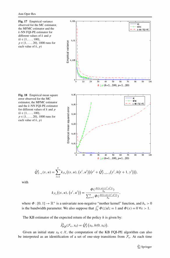
Fig. 16 Empirical averageobserved for the MC estimator,the MFMC estimator and thek-NN FQI-PE estimator fordifferent values of k and p
(k ∈ {1, . . . ,100},p ∈ {1, . . . ,20}, 1000 runs foreach value of k, p)
a uniform random distribution over the state action space. For each sample, we run theMFMC (resp. the k-NN FQI-PE estimator). As a baseline comparison, we also compute1000 runs of the MC estimator for every value of p. Figure 16 (resp. 17 and 18) reportsthe obtained empirical average (resp. variance and mean squared error).
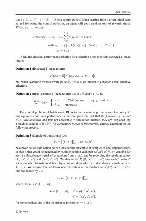
We observe in Fig. 16 that (i) the MFMC estimator with p ∈ {1, . . . ,3} is less biasedthan the k-NN FQI-PE estimator with any value of k ∈ {1, . . . ,100} and (ii) the bias of theMFMC estimator increases faster (with respect to p) than the bias of the k-NN FQI-PEestimator (with respect to k). The increase of the bias of the MFMC estimator with respectto p is suggested by Theorem 1, where an upper bound on the bias that increases with p isprovided. This phenomenon seems to affect the k-NN FQI-PE estimator (with respect to k)to a lesser extent. In Fig. 17, we observe that the k-NN FQI-PE estimator has a variance thatis higher than that of the MFMC estimator for any k = p. This may be explained by the factthat for samples of n = 100 transitions, one-step transitions are often re-used by the k-NNFQI-PE estimator, which generates dependence between artificial trajectories. We finallyplot in Fig. 18 the observed empirical mean squared error (sum of the squared empiricalbias and empirical variance) and observe that in our specific setting, the MFMC estimatoroffers for values of p ∈ {1,2,3,4} a better bias versus variance compromise than the k-NNFQI-PE estimator with any value of k.
5.3 Kernel-based and other averaging-type regression algorithms
The results exposed in Sect. 5.2 can be extended to the case where the FQI-PE algorithmis combined with kernel-based regressors and in particular tree-based regressors. In such acontext, the sequence of functions (Qh
T −t (.))Tt=0 is computed as follows:
Definition 23 (KB FQI-PE algorithm)
• ∀(x,u) ∈ X × U ,
Qh0(x,u) = 0.
• For t = T − 1, . . . ,0, ∀(x,u) ∈ X × U ,
Ann Oper Res
Fig. 17 Empirical varianceobserved for the MC estimator,the MFMC estimator and thek-NN FQI-PE estimator fordifferent values of k and p
(k ∈ {1, . . . ,100},p ∈ {1, . . . ,20}, 1000 runs foreach value of k, p)
Fig. 18 Empirical mean squareerror observed for the MCestimator, the MFMC estimatorand the k-NN FQI-PE estimatorfor different values of k and p
(k ∈ {1, . . . ,100},p ∈ {1, . . . ,20}, 1000 runs foreach value of k, p)
QhT −t (x, u) =
n∑
l=1
kFn
((x,u),
(xl, ul
))(rl + Qh
T −t−1
(yl, h
(t + 1, yl
))),
with
kFn
((x,u),
(xl, ul
)) = Φ(Δ((x,u),(xl ,ul ))
bn)
∑n
i=1 Φ(Δ((x,u),(xi ,ui ))
bn),
where Φ : [0,1] → R+ is a univariate non-negative “mother kernel” function, and bn > 0
is the bandwidth parameter. We also suppose that∫ 1
0 Φ(z)dz = 1 and Φ(x) = 0 ∀x > 1.
The KB estimator of the expected return of the policy h is given by:
J hFQI(Fn, x0) = Qh
T
(x0, h(0, x0)
).
Given an initial state x0 ∈ X , the computation of the KB FQI-PE algorithm can alsobe interpreted as an identification of a set of one-step transitions from Fn. At each time

Ann Oper Res
Fig. 19 Illustration of the KB FQI-PE algorithm in terms of artificial trajectories
step t , all the one-step transitions (xl, ul, rl, yl) that are not farther than a distance bn from(xt , h(t, xt )) are selected and weighted with a distance dependent factor. Other one-steptransitions are weighted with a factor equal to zero. This process is iterated with the outputof each selected one-step transitions. An illustration is given in Fig. 19. The value returnedby the KB estimator can be expressed as follows:
Proposition 7
J hFQI(Fn, x0) =
n∑
i0=1
. . .
n∑
iT −1=1
θ0,i00 θ
i0,i11 . . . θ
iT −2,iT −1T −1
(ri0 + · · · + riT −1
)
with
θ0,i00 = kFn
((x0, h(0, x0)
),(xi0 , ui0
)),
θit ,it+1t+1 = kFn
((yit , h
(t + 1, yit
)),(xit+1 , uit+1
)), ∀t ∈ {0, . . . , T − 2}.
Proof We propose to prove by induction the property
Ht : J hFQI(Fn, x0)
=(
n∑
i0=1
. . .
n∑
it=1
θ0,i0θ i0,i1 . . . θ it−1,it(ri0 + · · · + rit−1 + Qh
T −t
(yit−1 , h
(t, yit−1
))))
.
Basis: One has
J hFQI(Fn, x0) =
n∑
i0=1
θ0,i0(ri0 + Qh
T −1
(yi0 , h
(1, yi0
))),
which proves H1.
Induction step: Let us assume that Ht is true for t ∈ {1, . . . , T − 1}. Then, one has

Ann Oper Res
J hFQI(Fn, x0)
=(
n∑
i0=1
. . .
n∑
it=1
θ0,i0θ i0,i1 . . . θ it−2,it−1(ri0 + · · · + rit−1 + Qh
T −t
(yit−1 , h
(t, yit−1
))))
.
(6)
According to the KB value iteration algorithm, we have:
QhT −t
(yit−1 , h
(t, yit−1
)) =k∑
it+1=1
θ it−1,it(rit + Qh
T −t−1
(yit , h
(t + 1, yit
))). (7)
Equations (6) and (7) give
J hFQI(Fn, x0) =
n∑
i0=1
. . .
n∑
it−1=1
θ0,i0 . . . θ it−2,it−1
×(
ri0 + · · · + rit−1 +n∑
it =1
θ it−1,it(rit + Qh
T −t−1
(yit , h
(t + 1, yit
))))
.
Since∑n
it =1 θ it−1,it = 1, one has
J hFQI(Fn, x0) =
n∑
i0=1
. . .
n∑
it−1=1
θ0,i0 . . . θ it−2,it−1
×(
n∑
it =1
θ it−1,it
)(ri0 + · · · + rit−1
)
+n∑
it=1
θ it−1,it(rit + Qh
T −t−1
(yit , h
(t + 1, yit
)))
=n∑
i0=1
. . .
n∑
it−1=1
θ0,i0 . . . θ it−2,it−1
n∑
it =1
θ it−1,it
× (ri0 + · · · + rit−1 + rit + Qh
T −t−1
(yit , h
(t + 1, yit
)))
which proves Ht+1. The proof is completed by observing that Qh0(x,u) = 0, ∀(x,u) ∈
X × U . �
One can observe through Proposition 7 that the computation of the KB estimate of theexpected return of the policy h can be expressed in the form of a weighted sum of the returnof nT artificial trajectories. Each artificial trajectory
[(xi0 , ui0 , ri0 , yi0
),(xi1 , ui1 , ri1 , yi1
), . . . ,
(xiT −1 , uiT −1 , riT −1 , yiT −1
)]
is weighted with a factor θ0,i00 θ
i0,i11 . . . θ
iT −2,iT −1T −1 . Note that some of these factors can even-
tually be equal to zero. Similarly to the k-NN estimator, these artificial trajectories are alsobuilt from the T × nT non-unique one-step system transitions from Fn.
More generally, we believe that the notion of artificial trajectory could also be usedto characterize other batch mode RL algorithms that rely on other kinds of “averaging”schemes (Gordon 1995).

Ann Oper Res
6 Conclusion
In this paper we have revisited recent works based on the idea of synthesizing artificialtrajectories in the context of batch mode reinforcement learning problems. This paradigmshows to be of value in order to construct novel algorithms and performance analysis tech-niques. We think that it is of interest to revisit in this light the existing batch mode rein-forcement algorithms based on function approximators in order to analyze their behaviorand possibly create new variants presenting interesting performance guarantees.
Acknowledgements Raphael Fonteneau is a Post-doctoral Fellow of the F.R.S.-FNRS. This paper presentsresearch results of the European excellence network PASCAL2 and of the Belgian Network DYSCO, fundedby the Interuniversity Attraction Poles Programme, initiated by the Belgian State, Science Policy Office.We also acknowledge financial support from NIH grants P50 DA10075 and R01 MH080015. The scientificresponsibility rests with its authors.
References
Antos, A., Munos, R., & Szepesvári, C. (2007). Fitted Q-iteration in continuous action space MDPs. InAdvances in neural information processing systems (NIPS) (Vol. 20).
Bellman, R. (1957). Dynamic programming. Princeton: Princeton University Press.Bonarini, A., Caccia, C., Lazaric, A., & Restelli, M. (2008). Batch reinforcement learning for controlling a
mobile wheeled pendulum robot. In Artificial intelligence in theory and practice II (pp. 151–160).Boyan, J. (2005). Technical update: least-squares temporal difference learning. Machine Learning, 49, 233–
246.Boyan, J., & Moore, A. (1995). Generalization in reinforcement learning: safely approximating the value
function. In Advances in neural information processing systems (NIPS) (Vol. 7, pp. 369–376). Denver:MIT Press.
Bradtke, S., & Barto, A. (1996). Linear least-squares algorithms for temporal difference learning. MachineLearning, 22, 33–57.
Busoniu, L., Babuska, R., De Schutter, B., & Ernst, D. (2010). Reinforcement learning and dynamic pro-gramming using function approximators. London: Taylor & Francis/CRC Press.
Castelletti, A., de Rigo, D., Rizzoli, A., Soncini-Sessa, R., & Weber, E. (2007). Neuro-dynamic programmingfor designing water reservoir network management policies. Control Engineering Practice, 15(8), 1031–1038.
Castelletti, A., Galelli, S., Restelli, M., & Soncini-Sessa, R. (2010). Tree-based reinforcement learning foroptimal water reservoir operation. Water Resources Research, 46, W09507.
Chakraborty, B., Strecher, V., & Murphy, S. (2008). Bias correction and confidence intervals for fittedQ-iteration. In Workshop on model uncertainty and risk in reinforcement learning (NIPS), Whistler,Canada.
Defourny, B., Ernst, D., & Wehenkel, L. (2008). Risk-aware decision making and dynamic programming. InWorkshop on model uncertainty and risk in reinforcement learning (NIPS), Whistler, Canada.
Ernst, D., Geurts, P., & Wehenkel, L. (2003). Iteratively extending time horizon reinforcement learning. InEuropean conference on machine learning (ECML) (pp. 96–107).
Ernst, D., Geurts, P., & Wehenkel, L. (2005). Tree-based batch mode reinforcement learning. Journal ofMachine Learning Research, 6, 503–556.
Ernst, D., Marée, R., & Wehenkel, L. (2006a). Reinforcement learning with raw image pixels as state input(IWICPAS). In Lecture notes in computer science: Vol. 4153. International workshop on intelligentcomputing in pattern analysis/synthesis (pp. 446–454).
Ernst, D., Stan, G., Goncalves, J., & Wehenkel, L. (2006b). Clinical data based optimal STI strategies for HIV:a reinforcement learning approach. In Machine learning conference of Belgium and the Netherlands(BeNeLearn) (pp. 65–72).
Ernst, D., Glavic, M., Capitanescu, F., & Wehenkel, L. (2009). Reinforcement learning versus model pre-dictive control: a comparison on a power system problem. IEEE Transactions on Systems, Man andCybernetics. Part B. Cybernetics, 39, 517–529.
Farahmand, A., Ghavamzadeh, M., Szepesvári, C., & Mannor, S. (2008). Regularized fitted q-iteration: ap-plication to planning. In S. Girgin, M. Loth, R. Munos, P. Preux, & D. Ryabko (Eds.), Lecture notes incomputer science: Vol. 5323. Recent advances in reinforcement learning (pp. 55–68). Berlin/Heidelberg:Springer.

Ann Oper Res
Fonteneau, R. (2011). Contributions to batch mode reinforcement learning. Ph.D. thesis, University of Liège.Fonteneau, R., Murphy, S., Wehenkel, L., & Ernst, D. (2009). Inferring bounds on the performance of a
control policy from a sample of trajectories. In IEEE symposium on adaptive dynamic programmingand reinforcement learning (ADPRL), Nashville, TN, USA.
Fonteneau, R., Murphy, S., Wehenkel, L., & Ernst, D. (2010a). A cautious approach to generalization in rein-forcement learning. In Second international conference on agents and artificial intelligence (ICAART),Valencia, Spain.
Fonteneau, R., Murphy, S., Wehenkel, L., & Ernst, D. (2010b). Generating informative trajectories by usingbounds on the return of control policies. In Workshop on active learning and experimental design 2010(in conjunction with AISTATS 2010).
Fonteneau, R., Murphy, S., Wehenkel, L., & Ernst, D. (2010c). Model-free Monte Carlo-like policy evalua-tion. In JMLR: W&CP: Vol. 9. Thirteenth international conference on artificial intelligence and statistics(AISTATS) (pp. 217–224). Laguna: Chia.
Fonteneau, R., Murphy, S. A., Wehenkel, L., & Ernst, D. (2010d). Towards min max generalization in rein-forcement learning. In Communications in computer and information science (CCIS): Vol. 129. Revisedselected papers. agents and artificial intelligence: international conference (ICAART 2010), Valencia,Spain (pp. 61–77). Heidelberg: Springer.
Gordon, G. (1995). Stable function approximation in dynamic programming. In Twelfth international confer-ence on machine learning (ICML) (pp. 261–268).
Gordon, G. (1999). Approximate solutions to Markov decision processes. Ph.D. thesis, Carnegie Mellon Uni-versity.
Guez, A., Vincent, R., Avoli, M., & Pineau, J. (2008). Adaptive treatment of epilepsy via batch-mode rein-forcement learning. In Innovative applications of artificial intelligence (IAAI).
Lagoudakis, M., & Parr, R. (2003). Least-squares policy iteration. Journal of Machine Learning Research, 4,1107–1149.
Lange, S., & Riedmiller, M. (2010). Deep learning of visual control policies. In European symposium on ar-tificial neural networks, computational intelligence and machine learning (ESANN), Brugge, Belgium.
Lazaric, A., Ghavamzadeh, M., & Munos, R. (2010a). Finite-sample analysis of least-squares policy iteration(Tech. Rep.). SEQUEL (INRIA) Lille–Nord Europe.
Lazaric, A., Ghavamzadeh, M., & Munos, R. (2010b). Finite-sample analysis of LSTD. In Internationalconference on machine learning (ICML) (pp. 615–622).
Morimura, T., Sugiyama, M., Kashima, H., Hachiya, H., & Tanaka, T. (2010a). Nonparametric return densityestimation for reinforcement learning. In 27th international conference on machine learning (ICML),Haifa, Israel, June 21–25.
Morimura, T., Sugiyama, M., Kashima, H., Hachiya, H., & Tanaka, T. (2010b). Parametric return densityestimation for reinforcement learning. In 26th conference on uncertainty in artificial intelligence (UAI),Catalina Island, California, USA, Jul. 8–11 (pp. 368–375).
Munos, R., & Szepesvári, C. (2008). Finite-time bounds for fitted value iteration. Journal of Machine Learn-ing Research, 9, 815–857.
Murphy, S. (2003). Optimal dynamic treatment regimes. Journal of the Royal Statistical Society. Series B,65(2), 331–366.
Murphy, S., Van Der Laan, M., & Robins, J. (2001). Marginal mean models for dynamic regimes. Journal ofthe American Statistical Association, 96(456), 1410–1423.
Nedi, A., & Bertsekas, D. P. (2003). Least squares policy evaluation algorithms with linear function approxi-mation. Discrete Event Dynamic Systems, 13, 79–110. doi:10.1023/A:1022192903948.
Ormoneit, D., & Sen, S. (2002). Kernel-based reinforcement learning. Machine Learning, 49(2–3), 161–178.Peters, J., Vijayakumar, S., & Schaal, S. (2003). Reinforcement learning for humanoid robotics. In Third
IEEE-RAS international conference on humanoid robots (pp. 1–20). Citeseer.Pietquin, O., Tango, F., & Aras, R. (2011). Batch reinforcement learning for optimizing longitudinal driving
assistance strategies. In Computational intelligence in vehicles and transportation systems (CIVTS),2011 IEEE Symposium on (pp. 73–79). Los Alamitos: IEEE Comput. Soc.
Riedmiller, M. (2005). Neural fitted Q iteration—first experiences with a data efficient neural reinforce-ment learning method. In Sixteenth European conference on machine learning (ECML), Porto, Portugal(pp. 317–328).
Robins, J. (1986). A new approach to causal inference in mortality studies with a sustained exposure period–application to control of the healthy worker survivor effect. Mathematical Modelling, 7(9–12), 1393–1512.
Sutton, R. (1996). Generalization in reinforcement learning: successful examples using sparse coding. InAdvances in neural information processing systems (NIPS) (Vol. 8, pp. 1038–1044). Denver: MIT Press.
Sutton, R., & Barto, A. (1998). Reinforcement learning. Cambridge: MIT Press.

Ann Oper Res
Timmer, S., & Riedmiller, M. (2007). Fitted Q iteration with CMACs. In IEEE symposium on approximatedynamic programming and reinforcement learning (ADPRL) (pp. 1–8). Los Alamitos: IEEE Comput.Soc.
Tognetti, S., Savaresi, S., Spelta, C., & Restelli, M. (2009). Batch reinforcement learning for semi-active sus-pension control. In Control applications (CCA) & intelligent control (ISIC) (pp. 582–587). Los Alami-tos: IEEE Comput. Soc.