generic sensor modeling for modulation … sensor modeling for modulation transfer function (mtf)...

GENERIC SENSOR MODELING FOR MODULATION TRANSFER FUNCTION (MTF) ESTIMATION

Taeyoung Choi

Dennis L. Helder Image Processing Laboratory

South Dakota State University (SDSU) Electrical Engineering and Computer Science Department

Brookings, SD 57007 [email protected]

[email protected]

ABSTRACT

An imaging sensor’s spatial quality can be expressed by the system’s point spread function (PSF). The PSF of a pushbroom Charge-Coupled Device (CCD) satellite sensor was numerically modeled including contributions from optic, detector, sensor motion, and electronic components. Synthetic edge and pulse targets with various intensity levels were developed and then convolved with the generic sensor model to produce synthetic output images. The output images were processed by proposed MTF estimators to develop optimized intermediate MTF processing steps such as edge detection and interpolation. System and ground noise simulation was performed. As a result of these noise simulations, improved MTF estimation methods were developed and a minimum SNR value was suggested for confident MTF estimators.

INTRODUCTION

The modulation transfer function (MTF) has been used to estimate the spatial quality of linear, shift-invariant imaging systems in the frequency domain. The spatial domain equivalent is the point spread function (PSF). Many design attributes, such as optics, detectors, and electronics contribute to the overall MTF or PSF of the system. However, this two-dimensional function is difficult to obtain and various techniques has been developed to estimate it. Often only a one dimensional estimate of the line spread function (LSF) can be found. Traditionally, laboratory tests were performed using sinusoidal inputs, periodic bar patterns, point source signals, and x-ray beams passed through narrow slits to derive estimates for the system LSF (Coltman, 1954, Kaftandjian, 1996). The most frequently used method was a step edge technique, from which the imaging system’s Edge Spread Function (ESF) can be obtained (Tzannes, 1995, Cao, 2000, Helder, 2002 and 2003). Then the LSF can be easily calculated by differentiating the ESF. MTF is calculated as the normalized magnitude of the Fourier transform of the LSF. Often, specifications limit minimum values of the MTF at the Nyquist frequency. Another type of commonly used input is a step pulse, for which sensor’s Pulse Response Function (PRF) can be derived. In this case, the MTF is the ratio of the Fourier transform of the PRF to the Fourier transform of the ideal input pulse. However, if the pulse is extremely narrow, it can approximate a line target as used in Schowengerdt’s work (Schowengerdt, 1985). Because this technique may use a relatively smaller target size than the edge method, he performed an in-orbit, across-track MTF analysis of the Landsat 4 Thematic Mapper (TM) using the San Mateo bridge at the south end of San Francisco Bay as a line target. Since the TM resolution (30 m) was larger than the width of bridge (18.3 m), the Nyquist frequency of the Fourier transformed bridge pulse profile occurred before its first zero crossing point. The small target size caused noise problems which were reduced by interpolation of the power spectrum values. Rauchmiller’s work (Rauchmiller, 1988) presented a method for measuring the TM PSF using a two-dimensional array of black squares on a white sand surface. Within TM’s 30 m ground sample distance (GSD), each of 16 square targets had it’s own unique 0.25 GSD sub-pixel offsets from along- and cross-track offsets under an assumption that these offsets enabled sub-pixel sampling to avoid MTF aliasing. His results were verified with Markham’s spatial model which provided pre-launch PSF and measurements of the TM and multispectral scanner (MSS) (Markham, 1985). This PSF model had separate components such as optics, detector, and electronics. Storey utilized this PSF model to predict the Enhanced Thematic Mapper Plus’ (ETM+) MTF (Storey, 2001). The Lake Ponchartrain Causeway in Louisiana was used as a two-lane parallel pulse target which was modeled as two ideal parallel step pulses. The best fitting parameters between the output scenes and simulated profiles

Pecora 16 “Global Priorities in Land Remote Sensing” October 23 – 27, 2005 * Sioux Falls, South Dakota

1

yielded estimates of the system’s MTF values. Spatial quality was monitored over time in the panchromatic band by comparing to pre-launch values. Recent advent of commercial high spatial resolution satellites, such as IKONOS, Quickbird and Orbview, requires a reliable measure of spatial quality of sub-meter resolution products. The high resolution images from these sensors provides detailed information of a small portion of the Earth’s surface as compared to the 30-meter resolution and larger field of view of the Landsat satellites. MTF estimation for these high spatial resolution sensors was performed by Helder (Helder, 2002 and 2003). Several interpolation techniques and edge detection methods were developed to produce reasonable MTF results from an input target image. However, since these interpolation methods and edge detection methods are very sensitive and critical to accurate MTF estimation, further study of these methods was warranted.

Since there was a need for checking the performance on sub-steps of MTF estimators, such as edge detection techniques and interpolation methods, an artificial sensor was numerically constructed with known parameters. A pushbroom CCD-type generic sensor model was generated assuming simplified characteristics of optics, detector, motion, and electronic blurring. After defining a sensor model or PSF, it was convolved with synthetic edge and pulse targets using a sampling rate 20 times higher than the desired ground sample distance (GSD) to avoid aliasing effects. Then the sub-sampled output images were resampled to a nominal 1 m GSD and MTF processed according to their target types. The edge detection techniques and interpolation methods were tuned to produce the closest MTF profile compared to the known system MTF. Non-uniformity on the ground was modeled as the sum of two-dimensional multi-resolution white Gaussian noise images. Numerical and theoretical effects of convolution between this ground noise and the system PSF were tested. System noise was simply defined as white Gaussian noise added to the sensor’s final output image. A set of noisy targets were generated and processed by the edge MTF estimator which produced an estimated MTF and an SNR value for each input image. With these optimized estimators, ground and system noise simulations suggested minimum SNR values which can be used as thresholds for confident MTF estimates.

PROCEDURES

Generic Sensor Model Definition The generic sensor PSF consisted of the system’s optical and detector components, as well as motion and

electronic effects. Mathematically, the system PSF was defined as the spatial convolution of its components as described below

det( , ) ( , )* ( , )* ( , )* ( , )opt motion electronicsPSF x y PSF x y PSF x y PSF x y PSF x y= . (1)

The first component, optical PSF, represents the response of the sensor optics to a point source. Spatial energy is distributed over a small area on the focal plane due to the telescope optics and is often modeled as a two-dimensional Gaussian function.

2222 2/2/

21),( byax

opt eeba

yxPSF −−=π

(2)

The non-zero physical area of each detector also causes blurring. Each sensor is considered to be a square or rectangle area on which incoming energy produces an averaged response. Therefore, the size of the detector rectangle is a variable which is modeled by using the rectangle function as defined in Figure 1. Equation (3) shows the detector PSF and it is modeled as the spatial-domain product of two rectangle functions in orthogonal directions.

)/()/(),(det GIFOVyrectGIFOVxrectyxPSF = (3)

For pushbroom sensor systems such as Ikonos and Quickbird, motion of the sensor platform causes the focal plane to travel in the along-track direction. Since the detector array on the focal plane has an integration time in which to ‘capture’ the incident radiance, this motion introduces blurring. The blurring profile is modeled as a rectangle function in the along-track direction as shown below. The parameter ‘S’ represents the spatial distance traveled by the detector as projected to the ground during integration, and is simply a product of platform velocity and detector integration time.

( ) ( / )motionPSF y rect y S= (4)


2

Figure 1. Definition of rectangle function used in detector and motion PSF’s.

Because detector outputs are electronically low-pass filtered prior to sampling in order to reduce aliasing effects in typical imaging systems, this effect was modeled as a simple first order 2-D Butterworth lowpass filter (Schowenderdt, 1997):

2

0

),(1

1),(

⎥⎦

⎤⎢⎣

⎡+

=

DvuD

vuH (5)

Where D(u,v) is defined as

( )21

22),( vuvuD += (6)

Variables u and v represent Fourier domain horizontal and vertical frequency variables.

Generic sensor model generation Since the work described in this paper was driven by a need to develop accurate on-orbit MTF/PSF estimators

for commercial high spatial resolution satellites systems, the system PSF model was developed to closely mimic these sensors. Consequently, model parameters were chosen such that the overall Full-Width at Half Maximum (FWHM) estimate from the LSF was approximately 1.12 meters. A value of 0.39 was chosen for both optical parameters; the resulting FWHM was approximately 0.9 meters. The detector size was chosen such that the GIFOV covered 1 m2 on the ground. For motion PSF, a ‘worst-case’ blur width of 0.25 m with normalized amplitude of 0.06 was chosen. Finally, electronic PSF was designed according to (5) and (6), with a cut-off frequency of 1.4 cycles/pixel or cycles/meter. The FWHM of the electronics PSF was 0.25 m in the spatial domain in both orthogonal directions.

The system PSF was calculated as the convolution of all the sub-components in the spatial domain. System PSF was trimmed to a 5m x 5m square extent (corresponding to 200 x 200 pixels) for calculation convenience as shown in Figure 2. The along-track FWHM value was approximately 1.4 cm larger than across-track FWHM (Figure 2b and c) because the along-track direction had additional motion blurring. Fourier transformation was applied to these LSF’s and system MTF plots are shown in Figure 3. The motion blurring caused a barely noticeable lower MTF trend in the along-track direction.

-5 -4 -3 -2 -1 0 1 2 3 4 5-0.2

0

0.2

0.4

0.6

0.8

1

1.2FWHM plot - Normalied by the maximum value

Nor

mal

ized

val

ue

Pixel

FWHM = 1.2381 [Pixel]

-5 -4 -3 -2 -1 0 1 2 3 4 5-0.2

0

0.2

0.4

0.6

0.8

1

1.2FWHM plot - Normalied by the maximum value

Nor

mal

ized

val

ue

Pixel

FWHM = 1.2522 [Pixel]

(a) The system PSF (b) Along track LSF (c) Cross track LSF

Figure 2. The system PSF with along and cross track LSF. One pixel is one meter.


3

0 0.05 0.1 0.15 0.2 0.25 0.3 0.35 0.4 0.45 0.50

0.1

0.2

0.3

0.4

0.5

0.6

0.7

0.8

0.9

1

Cross-track PSF MTF @ Nyq.= 0.2684

Along-track PSF MTF @ Nyq.= 0.2589

Normalized frequency [cycle/pixel]

Nor

mal

ized

val

ue

MTF comparison in cross and along track direction

Cross-track MTF

Along-track MTF

Figure 3. MTF over plots in along and cross track direction

Synthetic target generation Synthetic targets were generated by defining a pulse or edge on a 1000 by 1000 sub-pixel (or 50 by 50 meter)

matrix oriented approximately six degrees from the vertical. The second step is the convolution of the matrix with the system PSF function. To obtain a final nominal image size of 40 x 40 pixels with 1 meter GSD requires sampling every 20th pixel both vertically and horizontally. Other sampling schemes can be used for desired GSDs. As an example, the top right corner of Figure 4 shows a 1000 x 1000 sub-pixel synthetic edge target. It is convolved with the generic sensor model to produce an 800 by 800 (or 40 by 40 meter) sub-sampled output edge image. This sub-sampled image was resampled to 1 meter GSD before it was used for MTF estimation.

Figure 4. Synthetic edge target generation

MTF estimation methods

A synthetic target, such as the edge target in Figure 4, which is applied to the system PSF through the convolution and resampling processes, contains full information of the sensor’s one-dimensional blurring characteristics. To estimate these spatial characteristics, two MTF measuring techniques were developed according to the ground target shapes. Representative edge and pulse MTF estimators are explained in this section with their common interpolation and edge detection techniques. However, these methods tend to under-estimate the sensor’s true MTF. Using this generic sensor model, improvements to the MTF estimator can be developed. Both edge and pulse target methods produce one-dimensional line spread functions and pulse response functions. These functions can be over-sampled by appropriate alignment of the target edge with respect to the vertical (or horizontal). However, in order to align each of these edge profiles, it is critically important to be able to locate the


4

edge with sub-pixel accuracy. The presence of noise in each row profile makes sub-pixel edge detection more difficult. Model-based edge detection was developed instead of using a more generic numerical calculation such as cubic polynomial fitting. The Fermi function was chosen by Tzannes (Tzannes, 1995) to represent the ESF as shown in (7).

d

cbx

axf +

⎥⎦⎤

⎢⎣⎡ −−

=1)(exp

)( (7)

The parameter ‘a’ is a scale factor, ‘b’ is the symmetry point, ‘c’ represents the transition rate, and ‘d’ is a bias level. Even though all the output parameters have important information (for example, the MTF is directly related to the ‘c’ value), only the ‘b’ value was needed for determination of the sub-pixel edge location. Since synthetic edge targets by definition are a straight line, any deviation from the line contains potential errors in the geometry of the image that can serve as another possible source of degradation to the final MTF estimation. To keep the original geometry, all the calculated sub-pixel edge locations were forced to be on a straight line instead of using the sub-pixel position calculated from the previous algorithm. Figure 5 shows the results of a least squares fit through the sub-pixel edge locations. The circles in the figure indicate edge locations in each row, and the solid line is the corresponding least squares fit. Once the edge location is determined for each row of data, the data can be plotted as a simple over-sampled edge profile with all rows aligned by their edge location in Figure 5b.

Test image

Pix

el

Pixel

Angle is 5.990 degrees

5 10 15 20 25 30 35 40

5

10

15

20

25

30

35

40

Sub-pixel edge location

Least square error line

-25 -20 -15 -10 -5 0 5 10 15 20 250

200

400

600

800

1000

1200Modified S-Golay interpolation with raw data

DN

Pixel

DNdiff

= 999.97STD

ave = 0.01

SNR = 79111.40

Raw data

Modified S-Golay filtering

(a) (b) Figure 5. An example of (a) edge detection, least square line fitting to the edge, and (b) the final

over-sampled edge profile.

Once the edge profiles have been aligned, it is normally necessary to smooth the data because of noise. This becomes a difficult task since it usually involves a filtering step that ultimately alters the final MTF estimate, and it is hard to know a priori which features to smooth and which should not be smoothed. This step is further complicated by the fact that the over-sampled edge profile data is not uniformly sampled. Thus, a filter is needed to both smooth the data appropriately and to resample it onto a uniform grid. Three approaches have been developed and simulated to achieve this task. The first method is the well-known cubic spline interpolation approach. The second approach, known here as the ‘sliding-window method’, fits a linear model to all the data within the width of a window (perhaps one pixel wide). The output at the center of the window is the value of the fit to the data at that point. Next, the window is moved an incremental amount to the right (0.05 pixel, for example) and the next output value is calculated. This process is repeated over the entire edge (or pulse) profile. The third approach uses a modified version of the Savitzky-Golay filter (Savitzky, 1964). Savitzky-Golay filtering is similar to the sliding-window method except that it uses a higher order polynomial to fit the data within the window. It was originally derived to be used on data that are equally spaced. Thus, in this implementation it needed to be modified for unequally spaced data. Hence the term is Modified Savitzky-Golay (MSG) filtering. Figure 6 shows implementation examples of the sliding-window method and the MSG method using a 4th order polynomial.


5

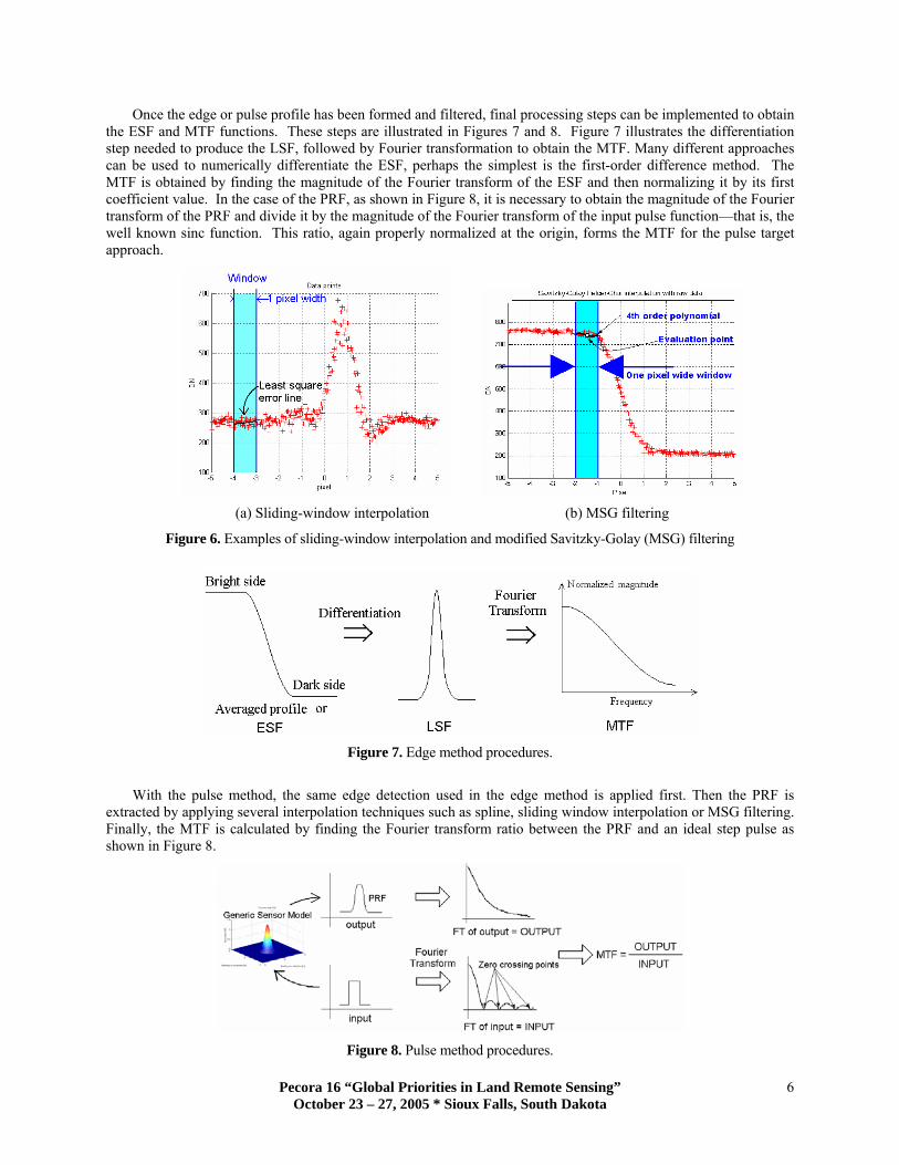
Once the edge or pulse profile has been formed and filtered, final processing steps can be implemented to obtain the ESF and MTF functions. These steps are illustrated in Figures 7 and 8. Figure 7 illustrates the differentiation step needed to produce the LSF, followed by Fourier transformation to obtain the MTF. Many different approaches can be used to numerically differentiate the ESF, perhaps the simplest is the first-order difference method. The MTF is obtained by finding the magnitude of the Fourier transform of the ESF and then normalizing it by its first coefficient value. In the case of the PRF, as shown in Figure 8, it is necessary to obtain the magnitude of the Fourier transform of the PRF and divide it by the magnitude of the Fourier transform of the input pulse function—that is, the well known sinc function. This ratio, again properly normalized at the origin, forms the MTF for the pulse target approach.

(a) Sliding-window interpolation (b) MSG filtering

Figure 6. Examples of sliding-window interpolation and modified Savitzky-Golay (MSG) filtering

Figure 7. Edge method procedures.

With the pulse method, the same edge detection used in the edge method is applied first. Then the PRF is extracted by applying several interpolation techniques such as spline, sliding window interpolation or MSG filtering. Finally, the MTF is calculated by finding the Fourier transform ratio between the PRF and an ideal step pulse as shown in Figure 8.

Figure 8. Pulse method procedures.


6

RESULTS

Performance of MTF estimation methods MTF estimators were implemented using spline interpolation, sliding-window interpolation, and MSG filtering

with noise-free synthetic edge and pulse images. Results for edge targets are presented in Figure 9 and Table 1. All estimators over-estimated FWHM values which resulted in under-estimation of MTF values at the Nyquist frequency. When compared to the known system MTF at Nyquist, spline interpolation under-estimated FWHM and MTF values by 21.6% and 51.9%. Although the sliding window interpolation produced closer values, the FWHM was 5.8% and MTF was 12.6% less than system values. MSG filtering produced the closest estimate to the system parameters. FWHM was 0.5% less than the known FWHM and the MTF value at Nyquist was 1.9% less than the system MTF. These results suggest that spline interpolation should not be used for MTF estimation because of large under-estimation errors up to 50%. However, though the sliding-window interpolation method performed better than spline interpolation, MSG filtering provided consistent results within two percent error in both spatial and Fourier domains.

Table 1. Edge method FWHM and MTF estimator results

Edge Method Model Spline Sliding MSG

LSF FWHM [m] 1.2380 1.5050 +21.6%

1.3100 +5.8%

1.2440 +0.5%

MTF at Nyquist 0.2684 0.1292 -51.9%

0.2347 -12.6%

0.2632 -1.9%

Figure 9. PSF and MTF estimates using the edge method

For the pulse method, all the interpolation and filtering methods also under-estimated FWHM and MTF values

compared to the true values. Interestingly, the range of FWHM estimates were smaller using the pulse as compared to the edge method. Although the largest difference occurred when spline interpolation was applied, the difference was only about 1.2% as shown in Table 2 and Figure 10. Both sliding window and MSG filtering produced FWHM estimates very close to the ground truth with differences of 0.26% and 0.07%, respectively. Similar to the edge method, the largest deviation occurred with spline interpolation resulting in 51% deviation from the original MTF value at Nyquist. Sliding window interpolation performed slightly worse than the MSG filtering method, producing 6.8% under-estimation. MSG filtering provided the best MTF estimation. From edge and pulse MTF estimator performance tests using the known sensor model, MSG filtering provided the most reliable MTF estimation in both spatial and frequency domains, whereas the sliding-window and spline interpolation methods showed large amounts of error. Since all these simulations were performed in a noise-free


7

situation, as mentioned earlier, there was a need to incorporate simulated MSG filtering and to insure accurate MTF estimations under less than ideal (i.e., noise-free) conditions.

Table 2. Pulse method FWHM and MTF estimator results

Pulse method Model Spline Sliding mSG

PRF FWHM [m] 3.0040 2.9670 (-1.23%)

2.9993 (-0.26%)

3.0020 (-0.07%)

MTF at Nyquist [cycle/pixel] 0.2684 0.1320

(-50.8%)0.2392

(-10.9%)0.2575 (-4.1%)

Figure 10. PSF and MTF estimates using the pulse target method.

Signal-to-Noise Ratio (SNR) Definition Prior to discussing system and ground noise simulations, SNR needs to be defined for pulse and edge targets.

Often, SNR is defined as the ratio of the mean value of an input signal to its standard deviation. For this analysis, a slightly different formulation is suggested that is consistent with the definition. The SNR definitions for the edge and pulse methods are shown in Figure 11. For an edge target, the signal was defined as the difference between the mean DN values of each region on either side of the edge. The standard deviation was calculated as the mean of the standard deviations of both regions. For pulse targets, the signal was defined as the difference between the PRF peak DN value and the mean background DN value. The standard deviation was defined as the standard deviation of the background excluding the pulse signal.

Figure 11. SNR definitions for edge and pulse profiles


8

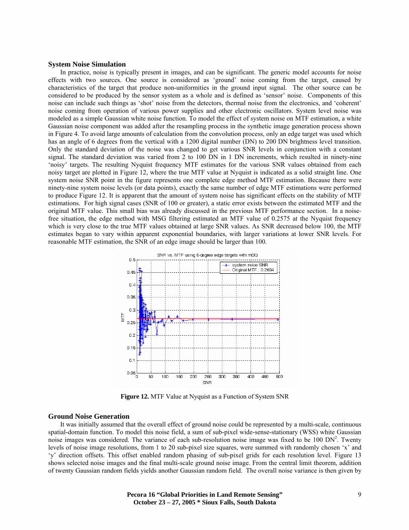
System Noise Simulation In practice, noise is typically present in images, and can be significant. The generic model accounts for noise

effects with two sources. One source is considered as ‘ground’ noise coming from the target, caused by characteristics of the target that produce non-uniformities in the ground input signal. The other source can be considered to be produced by the sensor system as a whole and is defined as ‘sensor’ noise. Components of this noise can include such things as ‘shot’ noise from the detectors, thermal noise from the electronics, and ‘coherent’ noise coming from operation of various power supplies and other electronic oscillators. System level noise was modeled as a simple Gaussian white noise function. To model the effect of system noise on MTF estimation, a white Gaussian noise component was added after the resampling process in the synthetic image generation process shown in Figure 4. To avoid large amounts of calculation from the convolution process, only an edge target was used which has an angle of 6 degrees from the vertical with a 1200 digital number (DN) to 200 DN brightness level transition. Only the standard deviation of the noise was changed to get various SNR levels in conjunction with a constant signal. The standard deviation was varied from 2 to 100 DN in 1 DN increments, which resulted in ninety-nine ‘noisy’ targets. The resulting Nyquist frequency MTF estimates for the various SNR values obtained from each noisy target are plotted in Figure 12, where the true MTF value at Nyquist is indicated as a solid straight line. One system noise SNR point in the figure represents one complete edge method MTF estimation. Because there were ninety-nine system noise levels (or data points), exactly the same number of edge MTF estimations were performed to produce Figure 12. It is apparent that the amount of system noise has significant effects on the stability of MTF estimations. For high signal cases (SNR of 100 or greater), a static error exists between the estimated MTF and the original MTF value. This small bias was already discussed in the previous MTF performance section. In a noise-free situation, the edge method with MSG filtering estimated an MTF value of 0.2575 at the Nyquist frequency which is very close to the true MTF values obtained at large SNR values. As SNR decreased below 100, the MTF estimates began to vary within apparent exponential boundaries, with larger variations at lower SNR levels. For reasonable MTF estimation, the SNR of an edge image should be larger than 100.

Figure 12. MTF Value at Nyquist as a Function of System SNR

Ground Noise Generation It was initially assumed that the overall effect of ground noise could be represented by a multi-scale, continuous

spatial-domain function. To model this noise field, a sum of sub-pixel wide-sense-stationary (WSS) white Gaussian noise images was considered. The variance of each sub-resolution noise image was fixed to be 100 DN2. Twenty levels of noise image resolutions, from 1 to 20 sub-pixel size squares, were summed with randomly chosen ‘x’ and ‘y’ direction offsets. This offset enabled random phasing of sub-pixel grids for each resolution level. Figure 13 shows selected noise images and the final multi-scale ground noise image. From the central limit theorem, addition of twenty Gaussian random fields yields another Gaussian random field. The overall noise variance is then given by


9

a linear sum of the individual variances. As a result of the addition process, the variance of the ground noise model was 2000 DN2.

Figure 13. Ground noise image examples. In this example, 1 pixel is equal to 5 cm, so the 20-pixel noise image has 1-

meter noise grain. Final composite image is shown at bottom right.

Ground noise simulation Noiseless edge images were derived with a variety of transition heights, as shown in Table 3, to simulate

varying signal amplitude. The multi-level ground noise image was added to the noiseless synthetic step edge images and the resultant noisy edge images were convolved with the two-dimensional system PSF. The output was resampled to a 1 m GSD, and then processed with the edge-based MTF estimator.

Table 3. Edge transition levels for ground noise simulation

Bright 1100 1000 950 900 850 825 800 790 780 775 770 Dark 400 500 550 600 650 675 700 710 720 725 730

Difference 700 500 400 300 200 150 100 80 60 50 40

The results of the ground noise simulation are presented in Figure 14. Asterisks represent the Nyquist frequency MTF estimates which are plotted versus estimated SNR from twenty independent simulations using each of the eleven pre-determined noisy edge images. The line is the true MTF of the sensor model. As might be expected, the MTF results for the ground noise simulation were similar to those observed for the system noise simulation shown in Figure 12. For SNR values greater than 100, the average MTF value was close to the theoretical MTF estimate, but exhibited a noticeable static bias as mentioned in the system noise section. Again, MTF estimates began to vary


10

noticeably for SNR values less than 100, with greater variation occurring for lower SNR values. These results also suggest that reliable MTF estimation can be achieved for SNR values of 100 or greater.

Figure 14. SNR vs. MTF value at Nyquist result plot from ground noise edge target simulation.

CONCLUSIONS

A pushbroom CCD sensor model has been developed to measure and improve performance of MTF estimation techniques. The sensor model was numerically defined by models of the optical PSF, detector PSF, motion PSF, and electronics PSF. An arbitrary 1 meter GSD sensor was utilized. With this known system PSF, the performance of MTF estimators was evaluated and significant improvement in their performance was obtained. Estimated MTF errors at Nyquist were significantly reduced by using MSG filtering and Fermi function edge detection; the resulting estimates differed from the true value by less than 2%. A combination of MSG filtering and Fermi function edge detection provided a reliable MTF result as compared to the other possible interpolation methods. System and ground noise simulations suggested a minimum threshold value of SNR ≥ 100 for confident MTF estimation with edge targets. The generic sensor model provided an excellent simulation environment to obtain artificial responses from various targets in the spatial domain. It is also a flexible spatial PSF modeling system adaptable to most CCD-based imaging systems using common system parameters.

ACKNOWLEDGEMENT

The authors with to thank colleagues from the JACIE team at Stennis Space Center for their support. This work was funded under NASA grant NAG13-03023.

REFERENCES Cao, X. (2000). A Novel Algorithm for Measuring the MTF of a Digital Radiographic System with a CCD Array

Detector. Medical imaging 2000, Proceedings of SPIE, 580-589. Coltman, J. (1954). The Specification of Imaging Properties by Response to a Sine Wave Input. Journal of the Optical

Society of America, 468-471. Kaftandjian, V. (1996). A Comparisons of the Ball, Wire, Edge, and Bar/Space Pattern Techniques for Modulation

Transfer Function Measurements of Linear X-Ray Detectors. Journal of X-ray Science and Technology, 205-221.


11

Markham, B. (1985). The Landsat Sensor’ Spatial Response,” IEEE Transactions on Geoscience and Remote Sensing, GE-23(6), 864-875.

Rauchmiller, R. (1988). Measurement of the Landsat Thematic Mapper modulation transfer function using an array of point sources. Optical Engineering, 27:334-343.

Savitzky, A. (1964). Smoothing and Differentiation of Data by Simplified Least Squares Procedures. Analytical Chemistry, 36:1627–1639.

Schowengerdt, R. (1985). Operational MTF for Landsat Thematic Mapper. SPIE Image Quality, 549:110-116. Storey, J. (2001) Landsat 7 on-orbit modulation transfer function estimation. SPIE Sensors, systems, and Next-

generation Satellites, 50-61. Tzannes, A. (1995). Measurement of the modulation transfer function of infrared cameras. Optical Engineering, 1808-

1817. Schowengerdt, R. (1997). Remote Sensing models and methods for image processing, Academic Press, 78-83. Helder, D. (2002). On-orbit Spatial Characterization of IKONOS. Proceedings of the 2002 High Spatial Resolution

Commercial Imagery Workshop, (CD-ROM). Helder, D. (2003). On-orbit Modulation Transfer Function Measurement of Quickbird. Proceedings of the 2003

High Spatial Resolution Commercial Imagery Workshop, (CD-ROM).


12

generic sensor modeling for modulation … sensor modeling for modulation transfer function (mtf)...

Documents