jensen modified sharpe fv1 - alpha power tradingalphapowertrading.com/jensen modified sharpe.pdfthe...

© Guy Roland Fleury, November 10, 2008 Last update: 17/03/2009 Page: 1

A Jensen Modified Sharpe Ratio to Improve Portfolio Performance.

ABSTRACT The main purpose of this paper is to reconcile my previous work on the modified Jensen alpha¹ methodology with the Stochastic Portfolio Theory as presented in Fernholz (2002). From the standard stochastic model, inclusion of the alpha enhanced method will show that it is possible to perform better than a market average or index fund (be it ranked by capitalization, Sharpe ratio or constant weights). The alpha feedback process will not only improve performance, it will also give the ability, to a certain degree, to better control a portfolio. No attempt is made to make an exhaustive proof of every assertion in this paper as the goal is not to produce an academic paper but to show that Stochastic Portfolio Theory (SPT), just as the Capital Asset Pricing Model (CAPM), can be used as stepping stones to higher portfolio performance. On the other hand, every attempt will be made to follow as closely as possible the mathematical notation as used in most of the academic papers I’ve read on this subject (see references for a partial listing). This paper at first presents an overview of the stochastic differential equation model as used in SPT. Then, the alpha accelerator is added to the portfolio process in order to improve performance. It is followed by a description of the trading environment and procedure implementation. Acknowledgements: Special thanks go to Murielle Northon for her support and to Murielle Gagné for keeping me on track while writing this paper. © Guy Roland Fleury, November 10, 2008. e-mail: [email protected] ____________ ¹ Alpha Power: Adding More Alpha to Portfolio Return. Available free from: http:/www.pimck.com/gfleury


Table of Content

1 The Stochastic Model 3 2 Ordered Performance 6 3 Revisiting the Jensen Alpha 7 4 Return to the Future 9 5 Designing a Trading System 9 6 Portfolio Weights 13 7 The Jensen Modified Sharpe 14 8 The Testing Environment 22 9 The Jensen Modified Sharpe II 25

10 The Trading System 26 11 Implementation 28 12 On the Growth Optimal Portfolio 35 13 Conclusion 37 References 39

© Guy Roland Fleury, November 10, 2008.


1. The Stochastic Model A stochastic representation of a portfolio of stocks could start with n + 1 assets being traded continuously. One asset being a bank account with a value process

)(0 tS , a terminal time horizon T , and satisfying the following differential equation:

dttStrtdS )()()( 00 = , [ ] 0)0(;,0 00 >=∈ sSTt (1)

where the fraction of capital, in cash or cash equivalent, 0s appreciates over time

at the bank’s interest rate )(⋅r which could be considered, in most cases, as the

risk free rate of return. The other n assets are stocks whose price processes satisfy the following stochastic differential equation (SDE):

,)()()()()(1

+= ∑

=

n

i

i

niiii tdWtdttbtStdS σ [ ] 0)0(;,0 >=∈ ii sSTt (2)

where )(tbi is the stock’s average rate of return (drift process); while )(tniσ being

the dispersion (or volatility) rate. )(tW i represent a standard n-dimensional

Weiner process with initial values 0)0( =iW , and where random influences can

be greater than the number of stocks by setting nj ≥ . From equation (2), we can

define the stock’s “instantaneous” rate of return as:

,)()()()(

)(

1

∑=

+=n

i

i

nii

i

i tdWtdttbtS

tdSσ [ ] 0)0(;,0 >=∈ ii sSTt (3)

By setting the excess rate of return as:

))'()(,...),()(),()((:)( 1 trtbtrtbtrtbtB nii −−−= + , for ni ,...,1=

)(tB then expresses the risk premium as the rate of return of the i-th stock minus

the risk free rate. From the Capital Asset Pricing Model (CAPM) is derived the reward to risk ratio or the market price of risk )(tθ :

[ ],,0,)(

)()( Tt

t

tBt ∈=

σθ

We can also look at the process )(tB as being regulated by market volatility )(tσ

and market price of risk such that:


[ ] ...,,0..),()()( saTteatBtt ∈=θσ (4)

which can be reformulated as:

)(

)()(

)(

)()(

t

trtb

t

tBt

σσθ

−== (5)

this in turn is the same as the definition for the Sharpe ratio. Adapting the above equation to Jensen’s (1968) added alpha formulation would result in:

)(

)()(

)(

)()(

t

trtb

t

tBt

σα

σα

θ+−

=+

= (6)

where α would represent the added return due to trading skills, privileged information or intuition of the portfolio manager. Jensen was trying to measure the knowledge and skill brought to the game by the portfolio manager. All he found, on average, was a negative alpha (-1.1%). No wonder it is often put aside and that practitioners mostly use the Sharpe ratio metric or its equivalents. Nonetheless, the Jensen alpha should be considered as a measure of what a portfolio manager brings as skill, knowledge, luck or trading methods to the game. And as such, it provides a measure of the performance achieved over and above the market’s average. It is only a small step from here to treat a market portfolio M simply as the sum of the individual stocks. Therefore, the sum of the incremental differences in value of each of the m stocks in the market will correspond to the total market portfolio incremental change:

,)()()()()(1,

+= ∑∑∑

=

m

mi

i

miii

m

i

i

m

i

tdWtdttbtStdS σ [ ] 0)0(;,0 >=∈ ii sSTt (7)

Equation (7) shows that the total incremental change in portfolio value is the sum of each stock’s drift, plus the cumulative sum of all their price variations. All this describes pretty well a portfolio model. In essence, we can represent any stock price as a regression line (its drift or rate of change) to which is added the cumulative sum of all random price variations. From equation (7), it is easy to deduce the average incremental change in portfolio value:

,)()()()(1

)(1

1,

+= ∑∑∑

=

m

mi

i

miii

m

i

i

m

i

tdWtdttbtSm

tdSm

σ [ ] 0)0(;,0 >=∈ ii sSTt (8)


As n (number of stocks in a portfolio) approaches m (number of stocks in the market universe); the portfolio will tend in value to the average market value:

)(1

)(1

tdSm

tdSn

m

i

m

i

n

i

n

i

∑

∑ mnas →→ 1 , a.s. (9)

which tends to show that the precepts of the Stochastic Portfolio Theory (SPT) will lead to an average performance at best. It is sufficient to pick about 30 stocks ( 30≥n ) from the universe of available stocks (m) to see expression (9) tend asymptotically to one. As if the simple fact of building a diversified portfolio condemns the portfolio holder to, at best, an average performance, almost surely. To outperform, one needs to either make a better selection than the average or trade in such a manner as to bring Jensen’s alpha into play. It’s the portfolio manager’s expertise that can make a difference and this is where a managed portfolio gains or looses relative value when compared to average performance. Trying to design a portfolio that has for objective to mimic the market average can only produce at best a portfolio that tends to the market average. The more you tend for average performance by design, the more you will get it. This is to say that equation (9) will tend to 1, almost surely, if the n stocks chosen for a portfolio tend to mimic the m stocks in the market universe. No one should be surprised of such a statement. Attempting, for instance, to maintain a stable Sharpe ratio )(⋅θ throughout the life

of a portfolio is akin to deliberately wanting to underperform. From equation (5) long term values for )(⋅σ and )(⋅r are relatively stable, this only leaves )(⋅b to

provide all the impetus for outperformance. And then, when the number of stocks n gets to 30 and above, the tendency for )(⋅b will be to tend to the average

secular market return. There seems to be no way out of this conundrum, the more you try to beat the averages, the more you get closer to the averages. It becomes the destiny of a long term portfolio to approach the secular market average asymptotically. The only recourse seems to pick n of the stocks that will outperform the market averages. And this becomes another problem altogether: which stocks should they be? By time slicing individual trades over the investment horizon, one will also observe that as the holding interval, for each trade, gets smaller and smaller, the number of trades will not only increase, but also the more and more performance will tend to the market average. As a matter of fact, performance will tend to be a little less than average due to incurred frictional costs.


2. Ordered Performance Using “order statistics” notation in decreasing order of return for )(⋅b , we can set:

)(min)(...)()(max)(1

21

1 tbtbtbtbtb ini

nini ≤≤≤≤

=≥≥≥= (10)

It becomes clear from (10) that the only desirable portfolio should be constituted of only one stock: )(1 tb (the one with the highest performance) and that all other

stocks will underperform this “atlas stock”. Being unable to select )(1 tb at portfolio

inception from the available stock universe, in the sense that the probability of picking )(1 tb tends to m/1 , other methods are required for the selection process.

Selecting a group of stocks having positive expectancy would appear as a reasonable alternative not counting the diversification benefits. But still the aim should be that the portfolio, when it reaches its terminal time horizon T, should be composed of stocks which should have had the highest possible returns )(⋅b .

However, this can hardly be done since no forecasting method could predict that far in the future with sufficient accuracy. Technically, all one can do is select, the best he/she can, n stocks from the m stock universe. Predicting what the price may be in 20 years is beyond the realm of any statistical or probabilistic methods. About all one could probably expect would be to find a general tendency for averages prices of the whole market universe to rise over the long haul. It might appear sufficient to select n stocks with the highest return from the available m stock universe, but even if it could be done, it still would not be enough. It would also be required that their weights in the portfolio be in the same order of precedence. This would require that )(tiπ the weight assigned to the i-th stock in the portfolio,

be in the same decreasing order as )(⋅b , namely:

)(min)(...)()(max)(1

21

1 ttttt ini

nini

πππππ≤≤≤≤

=≥≥≥= (11)

where 0)( ≥tiπ , 1)(1

=∑n

i tπ for all 0≥t , ni ,...,1=

Now, the task becomes even more complicated. Not only is it required to pick the highest performing stocks from a huge stock universe, but also, one has to put the heaviest weights on the top performers and tend as much as possible to put the heaviest weight on the atlas stock. In a sense, the game is deceptively simple: put all your money on the single best performing stock - the “atlas stock” - and you have achieved the highest possible return. And should you not be able to do so; then do the second best thing: that is to pick a number of the best performing


stocks with weights ordered by their relative performance. The portfolio rate of

return )(⋅πb would be the ordered weighted sum of stock returns:

)()()( tbttb ii

n

i

ππ ∑= (12)

which would by far exceed the market average being composed only of the highest performing stocks with an aggressive stance toward the best performers. The problem being, naturally, to realize such an objective knowing that price movements in the market can be considered as a quasi-random phenomenon. How is one to pick the best performing stocks and then assign weights in their order of relative performance? This is the real question! At a minimum, should one be unable to pick the best performing stocks, then all he/she could do would be to select a representative sample from the available stock universe. Then some means should be found to weight these stocks to their relative future performances. Again from the selected sample, weights should be ordered in decreasing order as in equation (11).

)()(min)()(...)()()()(max)()(1

221

11 tbttbttbttbttbt iini

nniini

πππππ≤≤≤≤

=≥≥≥=

where )()( 11 tbtπ would be the portfolio’s atlas stock and )()( tbt nnπ the less

desirable stock.

3. Revisiting the Jensen Alpha But before going into the details, there is a need to digress and elaborate more on the Jensen alpha (6). When Jensen formulated his equation, he saw the possibility for a portfolio manager to perform better than average and in doing so, produce a performance that was above the Capital Market Line (CML) for essentially the same risk in the risk-return space (see Figure 1). Jensen’s formulation of the expected portfolio return was a beta adjusted risk premium to which was added the risk free rate plus an alpha representing the portfolio’s overperformance (see Figure 1):

αβ +−+= ])([)( fmfp rRErRE

which is the equivalent to:

ασθ +⋅⋅+= )()()( fp rRE


Figure 1: Jensen’s Alpha

By adding alpha to the expected return equation, Jensen was giving a measurable value to the portfolio manager’s skills.

Not much can be made to change the average risk free rate of return. It has stood with an average of about 3.5% over the last century; as if that is all the market has to offer for idle funds. But Jensen opened up a door, in the sense that a portfolio manager that could generate some alpha was able to exceed the limitations of the CML. A talented portfolio manager could outperform the CML and this proportionally to his/her applied skills. In this sense, over performance was measurable and it had for name: alpha. It wasn’t specified which type of skills were applied (be it positive or negative), only that skills, talent, or luck (good or bad) could make a difference. When analysing the data, Jensen only found an average negative alpha (about -1.1%); meaning that the skills brought to the game by the average portfolio manager were detrimental to his performance. However, it should be noted that this minus 1.1% could be the results of such things as trading expenses, commissions and/or management fees applied against the portfolio. If this was so, then it would almost neutralize any alpha and establish that very little, if not no skill at all, was brought to the game as alpha would tend to zero. Technically, if Jensen was looking for portfolio management expertise across the financial investment industry; what he found was that only a select few could consistently exceed the averages while all others performed worst than average. It must have been disappointing for Jensen who, I think, wanted to positively prove that portfolio management skills mattered.


4. Return to the Future What ever market statistics we have for the past, they can only tell us what was. When considering the future, all these statistics paint a blurred and fuzzy image of what could be. It is only in general terms and using the conditional that one can express any equation related to future performance. The stochastic differential equations will still hold true, however no projection based on these equations would provide an explicit answer to how, when or what should be traded in the future. Already, some of the greatest tools have been made available to professional portfolio managers: computers, sophisticated software for data mining and analysis, gaming theory, artificial neural networks, genetic algorithms and anything else you can imagine; and yet, the average portfolio manager still does not beat the market averages; in fact, over 75% fail to beat the market average. Then, it might not be within the tools available that one should seek a solution to this portfolio management problem; maybe one should look at the trading methods used to outperform? If all the SPT literature point to a growth optimal portfolio as the most desirable, or most probable, outcome to long term portfolio management then it should come as no surprise that this optimal portfolio also tends to the weighted average of individual stock returns which in turn tends to the market average itself as ..samn →

It is not with equations (2) or (3), which can also explain the future, that you can design a trading strategy that will significantly outperform the seemingly inescapable market averages. It is by designing a total trading system that can capitalize on the market structure itself while having as prime objective not only to preserve capital but also produce appreciable positive alpha. The whole process therefore becomes a quest for generating positive alpha.

5. Designing a Trading System There we are: in need of designing a trading system. You have a mathematical model that explains pretty well the market you intend to trade. You have acquired knowledge of this market in statistical terms and have some basic equations as to the behaviour of stock prices. Your basic model tells you that there is a tendency for a long term upward drift to which is added a random variation component with an expected mean of zero (2). You have a whole lot of studies that tell you that the “efficient frontier” is in fact a boundary that is difficult to cross even by professional money managers. And your most probable outcome is to manage a portfolio that will tend toward the contact point on the CML tangent to the efficient frontier (see Figure 1). Technically, your only chance is to generate some alpha, but history has shown that portfolio managers fail, on average, to produce a positive alpha (Jensen 1968).


You have been shown the virtues of diversification, the merits of cutting your losses, the necessity of maintaining the capital under management above zero and that your portfolio should be self-financing. But all this does not design a system; it only provides some general guidelines. For example, in most cases, implementing stop losses will also tend to reduce overall performance. Thereby, one might be tempted to not use stop losses at all in order to obtain higher performance. However, we should consider this to be the cost to be paid as portfolio insurance and this cost can be seen in the systematic execution of stop losses. Capital preservation in all portfolios is the prime directive. Averaging down on stocks on their way to Chapter 11 is certainly not the way to achieve higher performance. Another way to represent a stock price model could be to express it as an initial holding value to which is added a constant drift (the slope of the regression line being the rate of return) plus the sum of all random variations, as in:

∑++=t

iii xtaStS i

1

0 )()( ε (13)

The cumulative sum of random variations will have for expected value: zero.

E 0)(1

=∑t

iε for 0≥t

Equation (13), when evaluating the past, has an exact solution where all

quantities are known: the initial stock holding, its average rate of return )(⋅ia over

the investment period t and the sum of all random fluctuations up to time t. But going forward, only the initial holding value can be known and this only if the time is 0=t . The long term projection of the future value of a stock is more than

uncertain; as time elapses, the projected range increases. This is like saying that in 20 year’s time, a stock could be somewhere between $0.00 and $1,000.00 with a 95% degree of accuracy. Not particularly useful. Therefore, in designing a trading system, one is confronted with many unknowns for which, even though we do have mathematical models that reflect the subject under study, they do not provide any means of accurately forecasting the future. To this, you add for objective to order all the stocks in a portfolio by rates of return and portfolio weights when you know quite well that there is no means to forecast future performance let alone performances in decreasing order. Notwithstanding, one can rebalance a portfolio at any future date based on what happened before and up to that point in time. In this sense, one can readjust portfolio weights based on generating functions on any criteria wished without


restriction. That this be profitable or not is another question. But the fact remains; one can readjust portfolio weights as long as the time is now. Building a portfolio that in time must supersede all others, being with the same stock selection or otherwise, will have to contend with some capital restrictions and constraints. First, trading at all times must be realistic: meaning that every single trade done during the life of the portfolio must be, not only marketable, but also executable. There is no flipping a million shares on the open or close every day. It means that every trade must be marketable; someone has to be present on the other side of the trade. Also, there is no selling at market of a large block of shares without affecting the price substantially. Slippage will have to be accounted for when trade size increases. A portfolio must stay with a positive holding value over the entire life of the portfolio in order to assure survivability, sustainability and self-financing. A portfolio must or might need to be self-financing as a requirement. Another aspect is that the trading strategy must be sustainable, in the sense that at no point in time must its survivability, marketability or realistic execution be compromised. It must allow for adding or subtracting funds at any time under reasonable time constraints. Portfolio performance is simply the product of a series of returns as in:

)1()1)(1()](/)(1[)( 21

1

k

k

bbbtZtdZb +⋅⋅⋅++=+=⋅ ∏ πππ

where a single 1−=kb will wipe out the entire portfolio no matter how long the

series has been. Having a major portion of one’s portfolio in a single disastrous position can be very detrimental to the portfolio’s health and objectives. In the Stochastic Portfolio Theory (SPT), when looking at the market, total capitalization is considered as a premise to market weights. Thereby, a portfolio

value πZ has for instantaneous rate of change:

)()()(

)()(

)(

)(

11

tdWdttbtS

tdSt

tZ

tdZ in

i

n

ni

n

i i

ii ∑∑

==

+== σπ ππ

π

(15)

with 1)0( =πZ ; portfolio rate of return: ∑=

=n

i

ii tbttb1

)()()( ππ and portfolio volatility

∑=

=n

i

ii tttni

1

)()()( σπσ π .


In SPT, the logarithmic change is used in order to express in linear form what is ordinarily an exponential function. So the differential equation for stock price process )(tSi would be:

∑+=n

i

i

niii tdWtdtttSd )()()()(log σγ (16)

where )(tiγ is the growth rate (average geometric rate of return) of the i-th stock.

Integrating this last function would result in:

])()()(exp[)(0

0 ∫∑∫ +=t

o

n

i

i

ni

t

i sdWsdssStS σγ (17)

However, using the holding value )(tS obfuscates some of the trading principles

when the share count is made equal to one in order to consider simpler equations to model the portfolio. A share count of 1 means that the total capitalization of a stock is considered in the value process )(⋅S . This has for

advantage that it becomes relatively easy to elaborate a benchmark or market portfolio as in:

)(...)()(

)(

)(

)()(

21 tStStS

tS

tS

tSt

m

iii +++

==µ > 0

where )(tiµ represents the relative capitalization of the i-th stock compared to

the whole market. And 1)(1

=∑=

m

i

i tµ for all 0≥t ; )(...)()()( 21 tStStStS m+++= .

Clearly )(⋅µ can be considered a portfolio process and can be called the “market

portfolio”. The usefulness of this notation is that one can recreate a benchmark: the market portfolio, since ownership of )(⋅µ has the same meaning as owning

the entire market space. Comparing the relative performance of a portfolio to a benchmark or to the market portfolio can be useful. For a stock )(tSi and portfolio η , the relative

return process )(tSi versus η is defined as: ))(/)(log( tZtSi η .

The portfolio M with weights mµµ ,...,1 defined by ))(...)(/()()( 1 tStStSt mii ++=µ for

mi ,...,1= is called the market portfolio, and the weights iµ are called the market

weights or the market capitalization weights. The market portfolio mSStZ ++= ...)( 1µ , represents the combined capitalisation of

all stocks in the market. Therefore, from )(/)()( tZtSt ii µµ = it follows that

))(/)(log()(log tZtSt ii µµ = which represents the relative return of the i-th stock to


the market portfolio. For portfolios π and η , the relative return process of π to η

can be defined as:

))(/)(log( tZtZ ηπ (18)

The relative return process of portfolio π to the market portfolio M would simply

be: ))(/)(log( tZtZ mπ .

So, there we have it: a mathematical model to represent stock behaviour, portfolios, indexes and markets where everything can be evaluated, compared and analysed. It all makes sense and theoretically can be used to better control one’s portfolio. As if by controlling the portfolio weights you had a solution to optimize a portfolio to any extent. Well, let’s see.

6. Portfolio Weights When looking at past data, SPT provides an exceptional framework to analyse performance as well as relative performance to any benchmark. It is when looking at the future that the image gets blurred. Nevertheless, by controlling portfolio weights, one can design trading systems that correspond to specific philosophies. The Buy & Hold portfolio can be implemented with an initial weighting nSStZ ++= ...)( 1π where the weights

0)( ,...,1 ≥= niiw are left to evolve as the market advances in time. Such a scenario

will in time reorder weights where the stock with the highest appreciation will have the heaviest weight while that stock with the lowest performance will have the lowest weight and even might be 0 in cases where the company goes bankrupt. The Buy & Hold strategy therefore orders weights by relative stock performance as in equation (10). This means that what ever your stock selection for a portfolio, at terminal time horizon T, weights will have changed from maybe an initial constant weight to an ordered by return set of weights. By trying to maintain a relatively constant Sharpe ratio ( c=⋅)(θ ) over the life of a

portfolio, weights will be periodically readjusted to rebalance the portfolio. In doing so, shares of advancing stocks will be partially sold as their prices go up and lagging stocks bought in order to rebalance the weights to maintain a constant Sharpe ratio. The method can at best produce average market returns. Its disadvantage is that the portfolio is gradually divesting itself of its best performers in the hope of achieving superior returns from the laggards. This sounds like: “let’s sell our best performers for a profit and increase our positions in our worst performers which will certainly rebound”. Worst performers (laggards) most of the time rebound, but sometimes, they don’t. And buying laggards has the same properties as averaging down and with the same pitfalls as trying to


catch a falling knife. At some point in time, you may be heavily invested in a stock going straight into Chapter 11. Maintaining a constant Sharpe ratio condemns a portfolio to the most probable average performance since that is what it seeks. Maintaining constants weights ( cwi =⋅)( ) throughout the life of the portfolio

suffers from the same symptoms as the constant Sharpe ratio scenario. To maintain the weights constant, it is required to partially sell best performers and increase positions in the laggards; again in the hope of achieving higher performance. The method distributes the risk as if all stocks were equal which they are not. Again, since this portfolio seeks average performance, it will find it. Another method would be to maintain portfolio weights in the same proportions at the market capitalization weights. By mimicking the weights of the market average, one should expect to achieve returns close to the market average (see equation 9). The more one designs trading strategies to resemble average market performance, the more these objectives will tend to be realized. A portfolio ranked by performance might have a better chance of producing excess return, but most often this is done in a limiting way as to tend to the efficient frontier and therefore an average performance. However, procedures can be selected whereby a portfolio will exhibit improved performance from inception. It will be within the trading philosophy itself by applying specific trading rules that the portfolio will prosper. For instance, never trading stocks below $15.00 will have for distinction of eliminating almost 99% of stocks that might go bankrupt and that might have been part of a portfolio. This way, using this simple procedure, 300 basis points (3%) can be added to overall portfolio return. This hints to other procedures that can improve portfolio performance by controlling either the selection process and/or the portfolio weights.

7. The Jensen Modified Sharpe The purpose of this paper is to show that portfolio weights should increase according to performance (11) (12). Rebalancing or readjustments should be done in favour of best performer and not against, and worst performers should have their weights decrease as their respective performances decrease. Doing so will generate a portfolio where not only weights will be ordered by relative performance (10) but also the stock’s holding values themselves.

nSSStZ +++= ...)( 21π ; with nSSS ≥≥≥ ,...,,, 21 , a.s.

and where the “atlas stock” )(1 ⋅S will have the highest holding value:


)(min)(...)()(max)(

12

11 tStStStStS i

nini

ni ≤≤≤≤=≥≥≥=

Furthermore, best performers should have reinforcement features to increase their weights, and all the while reducing the weights of the underperformers. This will have for tendency to increase relative weights towards the atlas stock. To implement this, it requires a different look at the SDE as proposed by the SPT. First, the price process )(⋅S must be expressed for what it really represents: a

quantity and a price, namely )()()( tPtQtS iii = . A quantity process of one for )(⋅Q

can be useful in describing a benchmark where total capitalization can be considered as a surrogate in designing a market average or index. However, a quantity of one will hide the fact that the quantity of shares (the inventory on hand) can also change in time. And, that often, a portfolio of stocks can be considered as an inventory management system where inventory can go up and down. Second, when comparing an ordinary portfolio to the whole market, even the relation: 0)(/)( →tZtZ µπ as the size of the market’s total capitalization )(tZµ is so

large. Third, the signal to noise ratio is such that the signal represents only a small fraction of the surrounding noise and the signal is almost completely drowned in this noise. Even though )(tZµ will maintain its definition, the portfolio

)(tZπ will be adapted to reflect the actual quantity traded. Therefore, portfolio

)(tZπ will from now on be defined as:

∑∑==

==n

i

ii

n

i

i tPtQtStZ11

)()()()(π (19)

Total cost of acquired shares can be expressed as: ∑l

ii tPtQ1

)]()([ , the sum of all

shares bought over time at their respective prices (including multiple purchases on the same day). While the current value of shares on hand can be expressed

as: ∑=

⋅l

i

ii tPtQ1

)()]([ : the sum of accumulated shares over time valued at the

current price. Only the accumulation or long side of the portfolio equation will be considered in this paper as the aim is only to show that performance can be improved by applying a Jensen modified Sharpe methodology to trading. Adding a day trading component to this methodology could also help improve performance just as adding a derivative component; however, neither will be covered for the time being. The purpose of the paper is only to show that using simple procedures can help escape the limitations of the efficient frontier. So, as a general expression, the total profit generated for this long only scenario is simply the difference between current holding value and its total cumulative costs to acquire the said shares:


∑∑∑ =−⋅==

profitstPtQTPtQn

i

ii

n

i

ii

11

)]()([)()]([ (20)

The portfolio rate of return )(⋅πb can be considered as total profits over total

cumulative costs (invested capital):

)(

)]()([

)]()([)()]([

1

11tb

tPtQ

tPtQTPtQ

n

i

ii

n

i

ii

n

i

ii

π=

−⋅

∑

∑∑

=

== (21)

The return process )(⋅ib , when the quantity is made equal to one, would results in:

)()0(

)0()(tb

P

PtPi

i

ii =−

(22)

as should be expected. But this hides what could be done with the quantity as

time evolves. Equation (22) could also be expressed as t

ii btb )1()( += ; an

ordinary compounded rate of return. Now consider what would happen when one puts the quantity of shares on a compounded rate as in:

t

ii

i

ii gtgQ

QtQ)1()(

)0(

)0()(+==

− (23)

then )(tgi becomes the appreciation rate of the number of shares in the stock

inventory. Expanding inventory as price appreciates would result in:

t

i

t

iii gbtgtb )1()1()()( ++= (24)

To do this would require a slight modification to equation (6) which is restated here:

)(

)()(

)(

)()(

t

trtb

t

tBt

σα

σα

θ+−

=+

=

with the desired modification to )(⋅α , this would result in:

)(

)1()()()(

t

trtbt

t

στα

θ++−

= (25)


where τ is the Jensen alpha appreciation rate. This means that the process )(⋅θ

can be put on an exponential curve. The implications can be far reaching for a portfolio manager. From an historically static measure of reward to risk ratio, he/she can now look forward to a more positive outlook where the measure of the skill level increase in time all by applying procedural techniques to enhance

performance. The alpha accelerator: t)1( τα + , is almost entirely responsible for

the accelerating Sharpe ratio. In log differential form, this would translate equation (16) in to:

∑=

++=n

i

i

niiii tdWtdttttSd1

* )()()]()([)(log σαγ (26)

where )(* ⋅iα is the logarithm of the added appreciation rate resulting from the

share accumulation program over time. This changes completely the limitations of the CML as shown in Figure 1; since Jensen’s alpha )(⋅α is being replaced by

an exponential function:

t

iii t )1()(* ταα +=

The possibility of having an exponential Sharpe ratio changes the nature of the game in a big way. And since the Jensen accelerator can be controlled, it can provide a new dimension to skills applied to portfolio performance. This is the first time to my knowledge that the Jensen alpha formulation is improved since 1968. A new dimension is being added, one can not only produce positive alpha, but can do so on an exponential curve; it has for secondary effect an exponential Sharpe ratio (see Figure 2). Never in the past has anyone every expressed such a statement. The acceleration rate iτ of individual stocks has for origin )()()( tbtkt iii =τ with

0)0( =ik ; and where ik represent the fraction of generated excess equity being

reinvested. Thereby, )(* ⋅iα forms part of a positive portfolio feedback loop in

equation (26). To implement such a trading strategy requires that )(⋅ib determines the rate of

ascent of a subordinator function following a Lévy process which has drift, diffusion and jump components; a continuous Lévy process being a Brownian motion with drift. Subordinators can serve as goal oriented conditional performance objectives functions; akin to portfolio behavioural regulators. They can guide and control certain desirable portfolio parameters and become portfolio generating functions.


The feedback loop created by )(* ⋅iα has for single mission to amplify portfolio

output, and this translates in to: increasing performance exponentially.

Figure 2: Modified Sharpe Ratio

The Sharpe ratio with an alpha accelerator shows improvement over time of the reward per unit of risk. Management skills do matter.

With the use of subordinator functions, behavioural regulators, enhancers and safety valves, one can design a portfolio having for objective the realisation of equation (25). Tests over the 50 stocks by 1,000 weeks showed an increasing Sharpe over the whole 19.2 year investment period (see my previous paper). The tests ran on 100 stocks by 2,000 weeks show that the exponential Sharpe tends to taper off between years 22 and 26, but nevertheless, stays at a high value. One of the major reasons for this phenomenon might be that no replacement was provided for bankrupt companies within the selected group of stocks, and therefore, fewer and fewer stocks were effectively responsible for total performance as time advanced. It is understandable that one might not be able to design an exponential Sharpe ratio that could be maintained indefinitely. Tests with replacements have not been implemented yet. However, having replacement for bankrupt companies, or increasing the number of stocks as time evolves, would have for effect to further increase performance as a lot of excess equity buildup goes unused as time progresses.


Figure 3: Controlling Lévy Process

A typical subordinator function controlling the evolution of the alpha modified Sharpe ratio. It remains a Lévy process with drift, jumps and Brownian motion.

The portfolio generating function will be a Lévy process with jumps, random motion and drift. These Lévy processes will try to maintain an ordered weighting scheme based on relative performance of each individual stock. Thereby, trying to maintain equation (12) as an ordered set in weighting )(⋅π and return )(⋅b .

)()()( tbttb ii

n

i

ππ ∑=

The stock accumulation process )(⋅Q being controlled at the portfolio level will

distribute excess equity resources by reinforcement in the order of individual stock performances. Higher performing stocks will achieve the highest weighting in the portfolio while non-performers will not only be starved of capital but will also have their relative weights diminished. The use of subordinator functions as controlling elements for the behaviour of portfolio weights enable the user not only to preset, but also, to modify weights in time according to either changing environmental conditions or changes in the objective functions. As if one could control and regulate performance by increasing or decreasing controlling functions. Under this weighting structure, it is not known which stocks will have the heaviest weights at terminal time T, only that at terminal time T, stocks will be ordered by


weights according to their relative performance. As an illustration of the phenomenon, see Figure 5.

Figure 4: Weighting Lévy Process Control

A typical weighting subordinator function controlling the evolution of portfolio weights. Another Lévy process with drift, jumps and Brownian motion.

Position sizing is a major concern throughout the portfolio’s lifetime. It’s by controlling the ongoing stock inventory within the limits of the subordinator functions and regulators that the portfolio can thrive and exceed the Buy & Hold methodology by a wide margin. Initial positions in the selected stocks as well as ongoing incremental bets will determine overall portfolio performance. This method does not suggest having all initial weights of equal value nor does it recommend having the same incremental bets for all stocks. Initial bets should be place in order of expected return and/or any belief which can provide some degree of conviction in one’s trading methodology. Incremental bets could easily follow goal oriented subordinator functions in order to better use excess equity buildup as it progresses in time which in turn would have for effect to increase performance.


Figure 5: Portfolio Weighting Distribution

The weighting distribution under the subordinator controlling functions might be known at portfolio inception. However, at terminal time T, weights will be ordered by bet size and

performance.

From logarithmic equation (26), which is recalled here:

∑++=n

i

i

niiii tdWtdttttSd )()()]()([)(log * σαγ

one could perform integration; this would transform equation (17) in to:

])()())()((exp[)(0

*

0 ∫∑∫ ++=t

o

n

i

i

ni

t

ii sdWsdsssStS σαγ (27)

where )(* siα can be seen to push performance higher. The portfolio growth rate to

which is added the alpha modified Sharpe growth rate will remain within the self-financing and survivability constraints as: )(tZπ > 0, for [ ]Tt ,0∈ a.s.; even though

some of the weights might drop to zero (as in bankrupt companies for instance).


8. The Testing Environment How should an accelerated alpha portfolio be tested without introducing biases? What would constitute a testing environment where no tricks, no statistical aberration or specially selected examples could be used to make the point? Biases can have for origin: the stock selection process itself, the selected period under test, the over-optimization and/or curve fitting to the desired scenario, the survivorship bias, the use of faulty data not to mention peeking. Using a Monte Carlo method would simply average out over the stock selection while randomly selecting stocks might not include delisted or bankrupt companies. In order to avoid all forms of biases, a randomly generated trading environment would be used. Result: no optimization possible, no curve fitting, no removal of undesirable or misbehaved stocks and no forecasting possible. By doing this, the desired testing environment would be unbiased; it would also be quite severe as every single test would be different and unique from one to the next. The system would have no memory of past configurations, stock selections and price behaviours. Every scenario would be different as if having its own and unique time line. The first series of tests were based on 50 stocks over 1,000 weeks (about 19.2 years), while the second set was on 100 stocks spanning 2,000 weeks (38.4 years). All the data was randomly generated: initial value, drift and random price variations. Stock prices were normalized to an initial value of 20 without loss of generality in order to treat all stocks the same. See original paper Alpha Power1 for the 50 by 1,000 week tests. As an example see Figure 6 where a sample of 20 stocks is shown - in order not to cloud the chart - with their linear regression lines from random origins to random terminal values. When the data is normalized as in Figure 7, all regression lines appear to fan out from the same origin. However, note that the rate of change in both charts is the same. Figure 7 is comparable to Figure 11 in Alpha Power1; and from both figures, it is clear that the highest sloping linear regression line is the most desirable stock. This stock, the “atlas stock” would be the only stock to invest in should we have known before hand that it would be the best performing stock of the investment period. However, nothing can help us determine this in advance. Not being able to pick the atlas stock for your portfolio, the next best thing would be to select a number of stocks and play the game as described in the horse race beginning on page 30 of Alpha Power1. The description of the bet management system for the horse race does present the same problem as managing the relative performance of each stock in the selected portfolio. ____________ ¹ Alpha Power: Adding More Alpha to Portfolio Return. Available free from: http:/www.pimck.com/gfleury


Figure 6: Random Linear Regressions

The distribution of linear regressions appears as an array of sticks thrown on a table.

Figure 7: Normalized Random Linear Regressions

Normalizing the data in Figure 6 makes the distribution of random lines to fan out from the same origin. The rate of change is the same in both figures.


On the first series of tests, each run was like selecting 50 stocks at random from an unlimited stock universe with no replacement. Each price series having independent paths with the possibility of up to 28% of the group going bankrupt in which case the then current holdings would be forfeited (lost). It should be noted that this level of bankruptcy is much higher than what could be expected playing the real market. No way of knowing which stocks would outperform, go bankrupt or just produce about average returns. Each test would be a unique run so that no two price series could ever be the same since no seed was being used in the random number generator. Hundreds of runs were performed in order to gather statistics and better understand overall behaviour since each run was unique, unpredictable and unduplicatable. No biases could develop under the imposed trading conditions: no over optimization, no curve fitting, no selection bias, no indicator preference, no indicator optimized value, and no same stocks in all tests. There was no survivorship problem either as all would be bankrupted stocks were part of the selection and could not be avoided, discarded or ignored. And no peeking at future data in any form was permitted. Each run being as if generating a probable future outcome which had no memory of its past and no knowledge of what was to come; as if each test had its own unique time line.

Figure 8: Random Stock Price Series

The graph shows a typical 1,000 period randomly generated price series with drift. The white noise or random component can be much more significant than the signal.


This resulted in an Excel file with some 500,000 cells populated with inter-related functions and equations. A simple re-calculation request would run a totally new and different test with the then set of controlling functions and parameters. Efforts were made to simulate a market as closely as possible. Price variations were made to follow a Paretian distribution (meaning allowing fat tails) rather than using a normal or Gaussian distribution. An average secular trend was set to approximate the 10% long term historical market average with dividend reinvestment. This amounted to an average of about $0.02 drift per day with no ability to profit short term due to the high noise level from the random fluctuations. Because of the fat tails, gaps and price jumps could occur in any of the price series and at any time (see Figure 8). If the subordinator functions, regulators, amplifiers and safety valves were to be of any use, they would have to survive and thrive in this hostile trading environment.

9. The Jensen Modified Sharpe II The Jensen modified Sharpe ratio can have a major impact on a trading strategy. However, it is not all trading strategies that can benefit from it. The design implications have long term portfolio horizons as backdrop; this is not a short term trading methodology.

)(

)1()()()(

t

trtbt

t

στα

θ++−

=

From restated equation (25) above, the accelerated alpha component with also add an exponential component to the Sharpe ratio. Having that )(⋅θ can be a portfolio generating function will imply that the

generated portfolio will be on an exponential curve as well. It then becomes a matter of how much alpha and at what rate can the portfolio grow. And what are some of the controlling parameters? Trading procedures can be preset to a generalized behavioural pattern where the outcome might not be known but where the conditional response to market variations have all been predetermined. This trading “philosophy” then dictates the generated positive alpha and the portfolio manager can determine the sustainable rate of growth based on available capital and risk constraints. This goes beyond Stochastic Portfolio Theory where a barrier is put in place called the Growth Optimal Portfolio which resides on the efficient frontier and which is generated by equation (4):


)()()( tbtt =θσ

The modified Sharpe ratio jumps over this barrier; not as a simple incremental improvement but with an exponential function. It leaves behind the “efficient frontier” to expand performance by removing the restraints imposed by other portfolio rebalancing methods. Equation (25) represents only a small incremental step to the existing Sharpe ratio; it builds on what is there by providing a better use of excess equity buildup. Naturally, not adding this exponential to equation (25) would reduce the expression to equation (4), the usual expression for the Sharpe ratio.

10. The Trading System

The “instantaneous” rate of change of the portfolio can be expressed as:

∑∑==

++==n

ji

j

jiii

n

i i

iii tdWtdtttb

tS

tPtQd

tZ

tZd

1,

*

1

)()()]()([)(

)]()([

)(

)(σαππ

π

(28) which results from the weighted sum of the relative change in value of each stock. This change in value can come from the average price appreciation and/or the average quantity increase to which is added the cumulative sum of all random price variations. Both forces are at work; and for a positive alpha, it is clear that

)()()(*

tbttb iii ≥+α a.s.

The portfolio logarithmic rate of return:

)]()()[()( * ttbttb iii

n

i

αππ +=∑ (29)

results from the weighted sum of the combined rates of increase. While the portfolio volatility would remain the weighted sum of individual stock volatility:

∑=

=n

i

ii tttni

1

)()()( σπσ π (30)

From equation (24), we could also rewrite the portfolio equation as:

t

i

it

i

in

i

btPgtQtZ )1)(()1)(()( 00

1

++= ∑=

π (31)

where the price is made to appreciate at t

ib )1( + and the quantity at t

ig )1( + .


The portfolio value could also be expressed as:

∑∑∑===

−+=n

i

iin

i

iin

i

ii tPtQtPtQPQtZ111

)]()([)()]([)(00

π

where the total portfolio value is the sum of the initial position established in each stock plus the current value of all stock holdings minus the total cost of acquiring the said shares, or alternatively, the value of initial holdings + total profits. The total profit expressed only as rates of return could be written as:

t

i

t

iii gbtgtb )1()1()()( ++= (24)

Thereby the expression for the portfolio would be:

t

i

it

i

in

bPgQtZ )1()1()( 00

1

++= ∑π

where the initial positions in the market grow in quantity and in price. As a simple example, consider a 10% rate of return with a quantity appreciation rate of 5%:

=++=++= 20

0

20

000 )10.01()05.01()1()1()(iit

i

it

i

i

i PQbPgQtS 17.8501

compared to the simple Buy & Hold strategy which would result in:

=+=++= 20

0000 )10.01()1()01()(iiii

PQbPQtS t

ii 6.7275

a 265% performance improvement. Increasing the quantity at the same rate as price (0.10) would result in: 45.2593: a 672% improvement over the Buy & Hold – rising to an overall portfolio return of 21%. It therefore becomes desirable not to ignore that the quantity on hand as well as the price can appreciate in time. And when one considers an alpha of 3 to 5%, one could push overall performance somewhere between 27 to 31%; and this is not yet a limitation, performance can improve still further as )(tgi can itself be a time varying function.

The feedback loop generated by the alpha accelerator t)1( τα + will increase

portfolio performance as part of the excess equity build-up is being used to reinforce the desirable objective: achieving higher performance. This also provides for a better use of equity as the portfolio evolves in time. By controlling position size by relative price performance, we can increase overall portfolio return.


11. Implementation Only a simple and trivial scenario will be considered as the aim is not to give a complete or ultimate trading methodology but to show that one can increase performance simply by applying the alpha accelerator as described in the previous sections. Implementing a Jensen modified Sharpe ratio portfolio requires to setup initial trading conditions as well as ongoing controlling functions: subordinators, regulators, amplifiers, enhancers and safety valves. This is done by determining initial stock allocation to the selected set of stocks. The stock selection process itself can be any reasonable method of choice. Since the long term view is the prevalent underlying theme of this methodology; stocks being selected should have positive expectancy of survival; this does not mean a survivorship guarantee, only that one has reasonable assumptions for longevity. Forget penny stocks and look for stocks with future positive prospects. It also does not mean that the selection you make will survive the whole investment period, only that you are trying to put all the chances on your side by selecting what you think might survive and prosper. Stocks that fail can always be replaced as long as the remaining portfolio value is above zero. Also, the impact of a bankrupt stock will greatly be reduced as the number of stocks in the portfolio increases; this being the main reason for performing tests on 50 stocks in the first place. This naive diversification represented an implicit protection. Once a selection is done, it is time to set initial betting conditions. This will be done for each stock in the selection; and the same procedure would be applied when adding new stocks to the list to replace failed ones. Since the whole procedure plays the diversification game, one could normalize all selected stocks in order to treat them all the same and then divide initial capital according to capital requirements for each of the stocks. Or inversely, divide available capital into the number of stocks in your selection. This allocation will be done later but for now we can still set the theoretical framework of the procedure. Let the following represent the sum of initial positions:

∑∑∑===

==n

i

n

i

n

i

i iiiisPqkS

1

0000

11

)0()0()0()0( ; 00 ≥i

s (32)

where

ik0 is a multiple of the initial trade basis

iq0 . The trade basis can be any

quantity of shares from one to as high as capital permits. However, too low a trade basis is not necessarily recommended as commission costs may become a major impediment to performance. Trade basis should preferably start at 100 shares or in tradable increments of 100 in order to avoid odd lots. This is not to say that a trade basis of 10 or 21 shares will not work, it will, but performance will also be commensurate. Only part of the available capital is being invested at


inception; the stock weights will sum to 1 only for the invested portion of the portfolio. Remaining or unused funds will stay in the bank earning )(⋅r . The basis

for determining i

k0 can be any method you wish but it was found to be more

useful to make it proportional to a conviction or belief system. The more convince you are that a stock is going to prevail (survive), the higher its relative trade basis should be. Also, the higher the forecasted or anticipated rate of return, the higher )(⋅k should be as well. The trade basis can also be changed in time to adapt to

trading conditions or changes to objectives functions or forecasts. Various indicator functions then take over control of the emerging portfolio. These indicator functions have for mission to set guiding barriers in order to lead the portfolio value in the direction of the desired goals (capital appreciation).

bq shares are added to the portfolio when indicator conditions are met. The

quantity bought will depend on the indicator condition, the conviction setting and the trade basis for adding shares )()( ⋅⋅ qak .

)()()()()( )}()({ tPtatkItPtq qtthtcb ≥=

Since an initial bet can be a small fraction of initial capital, maybe something in the order of 0.1% of available capital, a price decline after initial setup will only have a minor impact on overall portfolio value. Even a 50% drop on one stock might only represent a 0.05% drawdown in portfolio value. The sum of all stock acquisitions over the investment period will be:

)()()()()()}()({

1,1,

tPtatkItPtq iqitthtcj

v

ji

ib

v

jijj ≥

==∑∑ = (33)

The capital requirement to execute equation (33) can be predetermined and can have for structure a general binomial function such as:

cbxax ++2 where the maximum of its derivative will represent the minimum required capital to execute the preset trading policy. The whole betting system’s equation will determine the outcome. As the share accumulation progresses, more and more capital will be required up to its maximum from which, excess equity buildup will take the forefront. Figure 7 shows capital requirements over the investment period. The positive side representing money put in the market while the negative side shows money taken out of the market. The regression equation has a 0.99 correlation coefficient which means that the binomial fit is good and explains most of the data.


A relatively small initial position may be taken, and then, the stock has to prove itself worthy before any additional shares can be purchased. And after having reached its maximum capital infusion, it is required that the market itself pays for it all... As a simple trivial example – which is part of a family of such equations - I will use the following deterministic portfolio driving function:

0

2 )0772.1(295.1)235.1(2

Re Paixiaxa

qCap qqqq

q −+−+= (34)

where qCapRe is the required capital, x the trade level (price differential), qi the

initial quantity traded and qa the added or ongoing quantity that serves as trade

basis. The idea here is to provide a simple example, where some of the controlling and safety functions have been omitted in order not to cloud the issue.

Figure 7: Capital Requirements (Portfolio)

The average capital required to implement the modified Sharpe ratio strategy will reach a maximum in the early stage, taper off and then will become self-sustaining. Amounts above zero represent capital put in the market while negative values show amounts taken out of the market. The regression line shows that this is a power function which is characterized by its initial stock position plus its ongoing additional bets.


The total capital requirement is all predetermined by equation (34) which also represents the ongoing betting system. This betting system (trading strategy) is characterized by its initial price, the initial quantity of shares bought, and the incremental bets in relation to the incremental trade level reached. The derivative of qCapRe will provide the trade level at which the minimum capital requirement

is met to execute the preset scenario:

0235.1Re

=−+= qqq iaxadx

qCapd (35)

where )35.12(1

qq

q

aia

x −= as determined by the betting strategy; and 0PPx t −= .

Figure 8: Capital Requirements (first 50 levels)

The regression function with a correlation coefficient of 1 show that the regression fits the data. The regression equation determines the betting system used.

Amounts above zero represent capital put in the market while negative values show amounts taken out of the market. The regression line shows that this is a power function which is characterized by its initial stock position plus its ongoing additional bets.


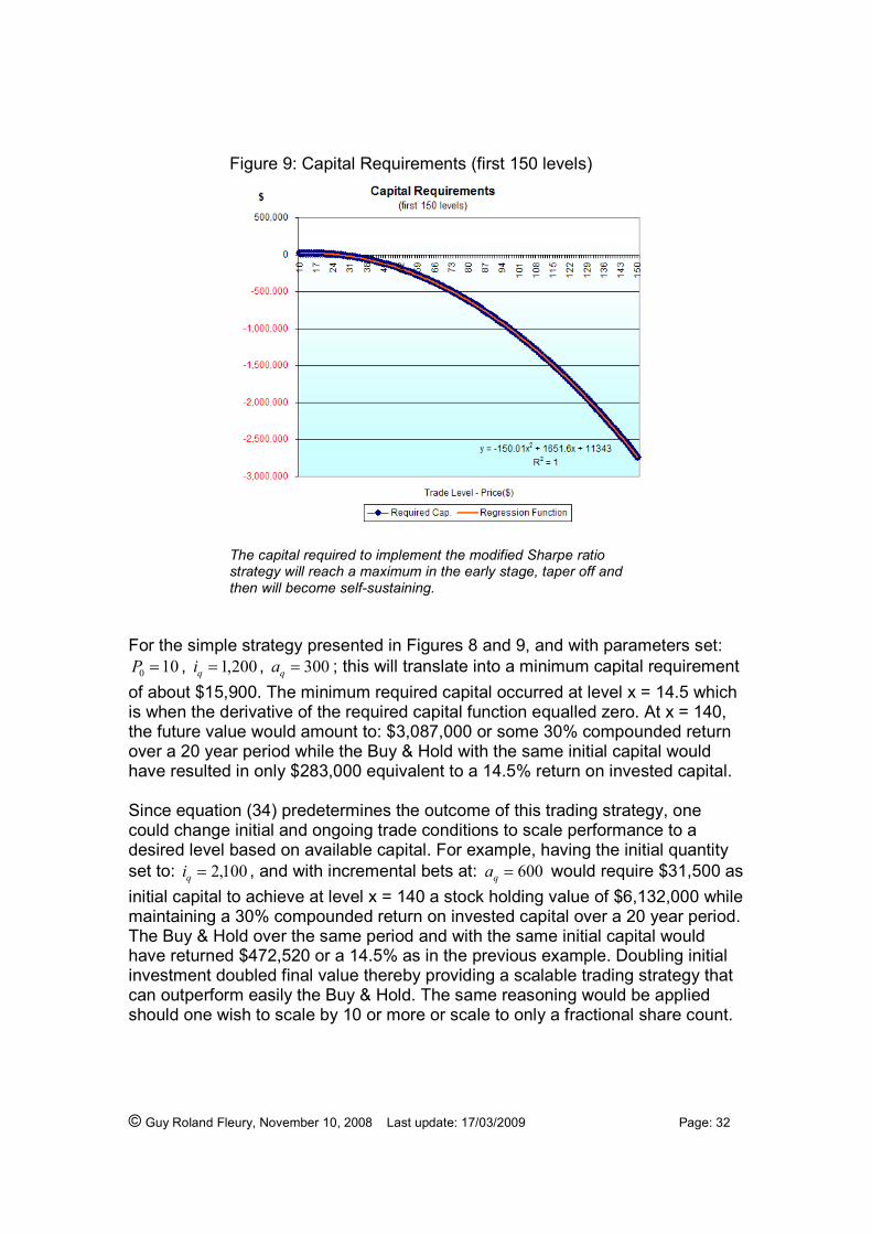
Figure 9: Capital Requirements (first 150 levels)

The capital required to implement the modified Sharpe ratio strategy will reach a maximum in the early stage, taper off and then will become self-sustaining.

For the simple strategy presented in Figures 8 and 9, and with parameters set:

100 =P , 200,1=qi , 300=qa ; this will translate into a minimum capital requirement

of about $15,900. The minimum required capital occurred at level x = 14.5 which is when the derivative of the required capital function equalled zero. At x = 140, the future value would amount to: $3,087,000 or some 30% compounded return over a 20 year period while the Buy & Hold with the same initial capital would have resulted in only $283,000 equivalent to a 14.5% return on invested capital. Since equation (34) predetermines the outcome of this trading strategy, one could change initial and ongoing trade conditions to scale performance to a desired level based on available capital. For example, having the initial quantity set to: 100,2=qi , and with incremental bets at: 600=qa would require $31,500 as

initial capital to achieve at level x = 140 a stock holding value of $6,132,000 while maintaining a 30% compounded return on invested capital over a 20 year period. The Buy & Hold over the same period and with the same initial capital would have returned $472,520 or a 14.5% as in the previous example. Doubling initial investment doubled final value thereby providing a scalable trading strategy that can outperform easily the Buy & Hold. The same reasoning would be applied should one wish to scale by 10 or more or scale to only a fractional share count.


Again from this simple example, one could extract the generated profits from the trading policy adopted. This would be expressed only in terms of initial price, initial bet, ongoing bets added as trade basis and trade level reached.

( ) ( ) ∑∑∑ =−−+−=− profitsPPpa

iPPpa

PQPQ oti

q

qoti

q

tttt )()2

()(2

2

Let ip equal one for now as to not cloud the issue. From the first scenario above,

the total profits would result in the following binomial equation (see Figure 10):

900750150 2 −+=∑ xxprofits

where ot PPx −= . To extract more profits, it is only required to scale the above

equation which will also increase the capital requirements accordingly. The number of shares acquired during the process can be evaluated using:

qotiqt iPPpaQ +−=∑ )(

which in this example, at level 140, would amount to 43,000 shares acquired over the 20 year investment period. When considering that one can buy shares with commissions as low as $1.00 per hundred shares, total commissions to realize the above scenario would amount to about $430.00 while the method would have produced total profits of about $ 3,087,000 or some 30% compounded return over the 20 year investment period. Commissions can really be considered a trivial matter when using this particular trading methodology. Equation (34) does indeed completely characterize this simple trading philosophy where all trading actions are predetermined. Any variation to this basic equation will also result in a predictable outcome. What is the minimum required capital to achieve $ 10,000,000 at the 140 level? Answer: $52,500 with optimal initial shares bought 500,3=qi shares and with additional bet size set at 000,1=qa .

Buying 1,000 additional shares as each trade threshold is reached is more than marketable and executable. This scenario would still produce as before over 30% compounded should the 140 level be reached at year 20. From a simple trading strategy where part of the excess equity buildup is used to reinforce the existing position at predetermined levels, it was shown that one could achieve higher performance without having to increase risk noticeably to do so. Equation (25) characterizes the trading philosophy. Whole families of curves as equation (34) can be designed and/or implemented.


Figure 10: Total Profit Generated (first 150 levels)

From the trading policy adopted, the sum of total profits originates from the current value of stock holdings minus the cost to acquire the said shares.

From the general background of SPT where every element tries to explain a quasi-random phenomenon, in occurrence: stock price movements, it was shown that one can design a deterministic trading methodology which will not only beat the Buy & Hold strategy, it can do so with little added risk. Not only that, but it is implied that whole families of such portfolio generating equations exists. Some of the advantages attributable to the methodology used in accumulating shares over the investment period would be:

a) only a relatively small initial investment is require as one can start with a small to zero initial commitment thereby limiting initial market exposure; since less than 5% of total equity can be put on initial bets, even with an average stock decline of 50%, it would represent only a 2.5% portfolio drawdown and a 0% decline should no initial positions be taken.

b) since shares are added only when the price is moving higher, one can always exit on this new high with all accumulated profits.


c) having a totally pre-determined trading plan with pre-set quantifiable goals helps to stay more focus in the face of market vagaries; you know where you want to go and you know how to get there, you just don’t know when you will get there, but you can wait. d) knowing in advance that the overall rate of return will be much higher than the Buy & Hold strategy provides more reasons to stay on course and reap the benefits of this progressive trading method. e) the method can be scaled by the initial position taken and ongoing bet size within the capital and risk constraints. f) stop losses are executed on small bets when negative and as trailing stops when profitable; meaning that when bets are larger, one can decide to keep most of the generated profits. This is not the same as accepting a huge loss. The decision process is very different. g) the method can be regulated by changing objective functions or modulated by market conditions. h) the method plays the diversification game and lets the fittest win the race.

The Jensen modified Sharpe ratio is a basis for a trading philosophy where instead of trying to outguess the market, one simply adopts a strategy to extract what he wants from the game.

12. On the Growth Optimal Portfolio

Where is the Growth Optimal Portfolio )(* ⋅π when )(* ⋅θ (its generating function)

goes from linear to exponential?

)(

)1()()()(

***

t

trtbt

t

στα

θ++−

= (36)

Under SPT )(* ⋅θ will generate a growth optimal portfolio )(* ⋅π that will tend

asymptotically to the market average as long term time horizons are considered. Since, with SPT, on long horizons, all terms of equation (5) are relatively constant, we could use secular averages as constants to roughly express )(⋅θ :


406.016.0

035.010.0

)(

)()()( =

−=

−=

t

trtbt

σθ

However, when considering the Jensen modified Sharpe ratio as in equation (36),

)(* ⋅θ is no longer a relative constant that can fluctuate within boundaries. It has

acquired an exponential component, a feedback loop, which will tend to increase the “optimal portfolio” exponentially (see Figure 2).

16.0

)1(035.010.0)(

***

t

tτα

θ++−

= (37)

Furthermore, *α and *τ could themselves be time varying functions modulated by market conditions or goal oriented functions. Leverage and margin can also be put to use in an effort to extract even more from the markets, just as adding a day trading component and/or derivative component would tend to increase performance further. Alpha can be generated by the simple use of part of the excess equity buildup generated as prices rise. Therefore, this method actually relies on buying shares incrementally as prices increase in time. And its added performance or overperformance simply originates from the use of the excess equity buildup. Equation (16) in my previous paper1 was its corner stone and did illustrate some of the controlling variables in the stock accumulation program. It was at the heart of my trading philosophy which transformed the simple Buy & Hold:

t

mrPQtH )1()( 00 +⋅⋅=

into a stock accumulation function with behavioural reinforcement of desirable characteristics:

t

m

t

m

b

arPxfra

afefsfQtH )1()()]1())(1()()()1[()( 0

1

0 ++⋅⋅⋅++++⋅⋅+⋅⋅⋅+⋅= −λψαζφ

The above equation is not a forecasting function but a predetermined inventory control function. It becomes how the quantity of shares on hand is being treated that counts. It’s the position sizing over the whole set of selected stocks that finally matters. It’s how the weights are shifted in time to favour the best performers while at the same time starving underperformers. At its most basic; the equation is a glorified Buy & Hold equation with the added twist of reinvesting in additional shares part of the accumulated excess equity under predetermined goal oriented functions which favour top performers. ____________ ¹ Alpha Power: Adding More Alpha to Portfolio Return. Available free from: http:/www.pimck.com/gfleury


It is also an equation which has a deterministic behaviour and where someone can preset objective functions based on capital and risk constraints. It’s output, the cumulated total profits can at times be express as a simple binomial equation as in the example presented above, such as:

CBxAxprofits −+=∑ 2 (38)

where A, B and C are functions of the betting system being implemented and require as information the initial bet size, the ongoing bet size (trade basis), its initial price and the price level reached. Without the betting system implied by this methodology, equation (38) would reduce to:

Dxprofits =∑ (39)

where D would be the initial shares bought qi ; and this in turn would be just

another expression for the Buy & Hold. The ability to convert a linear holding function to an exponential one through a simple deterministic procedure remains not only feasible but a desirable characteristic of the betting system implemented. From the capital constraints, a portfolio manager could design what is desired from a price movement, determine his/her behaviour in response to these price changes and set the betting strategy accordingly. Resolving the betting system’s equation (34), which sets the minimum capital requirements for execution, may seem the only requirement, but there is more. The betting system must be determined without knowledge of what is to come. The method, even though effective, will still not know what is coming as future price movements. But, nevertheless, it will make every attempt to maximize the output of the equation, in the sense that what ever the set of stocks thrown in the portfolio, it will make the best of it and produce returns that will exceed the Buy & Hold policy.

13. Conclusion From the backdrop of SPT, stock price, portfolio and market processes were represented as Stochastic Differential Equations. SPT is a complete market model, in the sense that it can represent any stock, market average, index or portfolio. From equation (17), an alpha accelerator was added to transform this equation in to equation (27). The alpha accelerator has for effect to increase performance and transform a relatively constant historical Sharpe ratio into an exponential one.

])()())()((exp[)(00

*

0 ∫∑∫ ++=t n

i

i

ni

t

ii sdWsdsssStS σαγ (27)


From what might be considered only a minor addition ( )(* siα ) to equation (27); it

turns out to have a major impact as it enables a portfolio to show an exponential Sharpe. Even with the trivial example provided, it was shown that one can design a better performing portfolio simply by reinvesting part of the excess equity buildup under controlled and deterministic inventory management procedures. Equation (27) is the corner stone of this paper, but all it does is restating in another form equation (16) in my previous paper.

The real innovation is still in my previous paper where for the first time the Sharpe ratio was given an exponential form (see equation (25)). The methodology aims to extract from the market following the capital requirement equation which sets the trading rules to achieve the preset profit objectives. It then becomes a matter of following the trading rules and possibly, if desired, to modulate equation parameters to changing objectives or market conditions. In essence, you design what you want to take out of the market and then let the market deliver on your terms.


References

Alemanni Barbara, Franzosi Alessandra. Portfolio and Psychology of High Frequency

Online Traders. March 2006.

Anderson Anders. Is Online Trading Gambling with Peanuts? March 2006.

Anderson Anders. All Guts, No Glory: Trading and Diversification among Online

Investors. April 2004.

Bachelier L. Théorie de la spéculation. 1900. Bain Alan. Stochastic Calculus.

Bank Peter, Baum Dietmar. Hedging and Portfolio Optimization in Financial Markets

with a Large Trader.

Banner Adrian D., Ghomrasni Raouf. Local Times Of Ranked Continuous

Semimartingales. December 2005.

Banner Adrian D., Fernholz Robert, Karatzas Ioannis. Atlas Models of Equity Markets. 2005.

Bansal Ravi, Dahlquist Magnus, Harvey Campbell R. Dynamic Trading Strategies and

Portfolio Choice. October 2004.

Barber Brad M., Lee Yi-Tsung, Liu Yu-Jane, Odean Terrance. Do Day Traders Make Money? January 2005.

Barber Brad M., Odean Terrance. All that Glitters: The Effect of Attention and News on

the Buying Behavior of Individual and Institutional Investors. September 2001.

Barber Brad M., Odean Terrance. Trading is Hazardous to Your Wealth: The Common

Stock Investment Performance of Individual Investors. June 1999.

Barberis Nicholas, Thaler Richard. A Survey of Behavioral Finance. September 2002.

Barberis Nicholas. Investing for the Long Run when Returns Are Predictable.

February 2000.

Barberis Nicholas, Huang Ming, Santos Tano. Prospect Theory and Asset Prices. June

1999. Barndorff-Nielsen Ole E. Financial volatility, Lévy processes and power variation. June

2002.


Berkelaar Arjan. Optimal Portfolio Choice Under Loss Aversion. December 2003.

Bjønnes Geir H., Holden Steinar, Rime Dagfinn, Solheim Haakon. ‘Large’ Vs. ‘Small’

Players: A Closer Look at The Dynamics of Speculative Attacks. March 2007. Bonney Lisa. Stochastic Portfolio Theory and its Applications to Equity Management.

MSc. Research Proposal. 2007.

Borodin Allan, El-Yaniv Ran, Gogan Vincent. Can We Learn to Beat the Best Stock?

Journal of Artificial Intelligence Research. 2004.

Bossaerts Peter, Plott Charles, Zame William R. Prices And Portfolio Choices In

Financial Markets: Theory, Econometrics, Experiments. July 2007.

Bouchaud Jean-Philippe, Gefen Yuval, Potters Marc, Wyart Matthieu. Fluctuations and response in financial markets: the subtle nature of ‘random’ price changes. July, 2003.

Breeden Douglas T. An Intertemporal Asset Pricing Model with Stochastic Consumption

and Investment Opportunities. July 1979.

Brennan Michael J., Xia Yihong. Persistence, Predictability, and Portfolio Planning.

September 2004.

Brennan Michael J., Wang Ashley W., Xia Yihong. Estimation and Test of a Simple

Model of Intertemporal Capital Asset Pricing.

Bywaters David, Thomas D. Gareth. Consumption, Wealth and Indebtedness in the

context of Uncertainty: The Consumption Function meets Portfolio Theory. University of

Hertfordshire Business School. Working Paper Series.

Campbell J. Y., Lo A. W. & MacKinlay A. C. (1996). The Econometrics of Financial

Markets, Princeton University Press, Princeton, NJ.

Cetin Coskun. Delegated Dynamic Portfolio Management Under Mean-Variance

Preferences. June 2006. Chamley Christophe. Complementarities in information acquisition with short-term

trades. 2007.

Chatterjee Sourav, Pal Soumik. A Phase Transition Behaviour for Brownian Motions

Interacting Through Their Ranks. June 2007.

Christensen Morten Mosegaard. On the history of the Growth Optimal Portfolio.

November 2005.


Christensen Morten Mosegaard, Platen Eckhard. When are Sharpe Ratio Based

Investments Superior? September 2005.

Christensen Morten Mosegaard, Platen Eckhard. Sharpe Ratio Maximization and

Expected Utility when Asset Prices have Jumps. November 2005. Cooper Michael, Gutierrez Jr. Roberto C., Marcum William. On the Predictability of

Stock Returns in Real Time. November 2001.

Cruset José. Analysis of Trend Following Systems. 2005.

De Giorgi Enrico, Hens Thorsten. Making Prospect Theory Fit for Finance.

December 2005.

Detko Kira, Ma Wilson, Morita Guy. Re-examining the Hidden Costs of the Stop-Loss.

Di Nunno Giulia. Lévy Random Fields: Stochastic Differentiation. Conference

August 2007.

Doney Ron. Fluctuation Theory for Lévy Processes. October 2005.

Dueker Michael J. Markov Switching in GARCH Processes and Mean Reverting Stock

Market Volatility. January 1997.

Elton Edwin J., Gruber Martin J. Modern portfolio theory, 1950 to date.

Journal of Banking & Finance 21 (1997) 1743-1759

Ericsson K. Anders, Andersson Patric, Cokely Edward T. The Enigma of Financial

Expertise: Superior and Reproducible Investment Performance in Efficient Markets.

September 2005.

Fama Eugene F. 1965. "The Behavior of Stock Market Prices." Journal of Business 37:

January 1965, pp 34-105.

Fama Eugene F. 1968. "Risk, Return, and Equilibrium: Some Clarifying Comments."

Journal of Finance 23: pp 29-40. Fama Eugene F. Random walks in stock market prices. Financial Analysts

Journal, Sep-Oct 1965.

Fernholz Robert, Maguire Cary, Jr. The statistics of ‘statistical arbitrage’ in stock markets.

December 2006.

Fernholz, R. Stochastic Portfolio Theory. 2002.

Fernholz, R. Equity Portfolios Generated by Functions of Ranked Markets Weights. 2001


Fernholz Robert, Karatzas Ioannis. Stochastic Portfolio Theory: an Overview. January

2008.

Fleury Guy Roland. Alpha Power: Adding More Alpha to Portfolio Return. October 2007. Franzoni Francesco, Marín José M. Portable Alphas from Pension Mispricing. October

2005.

Ghomrasni Raouf, Bonney Lisa. SDE in Random Population Growth. August 2008.

Ghomrasni Raouf. On Local Times of Ranked Continuous Semimartingales; Application

to Portfolio Generating Functions. June 2005.

Glaser Markus, Langer Thomas, Reynders Jens, Weber Martin. Framing Effects in Stock

Market Forecasts: The Difference Between Asking for Prices and Asking for Returns. February 2007.

Gollier Christian. Optimal Portfolio Management for Individual Pension Plans

Cesifo Working Paper No. 1394. February 2005

Gnedin Alexander, Pitman Jim and Yor Marc. Asymptotic laws for regenerative

compositions: gamma subordinators and the like. February 2008

Grinblatt Mark, Han Bing. Prospect Theory, Mental Accounting, and Momentum.

August 2004.

Grinold Richard C., Kahn Ronald N. Active Portfolio Management

Hansen Peter Reinhard, Lunde Asger. A Comparison of Volatility Models:

Does Anything Beat a GARCH(1,1)? March 2001.

Harlow W. V., Brown Keith C. The Right Answer to the Wrong Question: Identifying

Superior Active Portfolio Management. August 2005.

Hero Alfred O., Ma Bing, Michel Olivier, Gorman John. Alpha-Divergence for Classification, Indexing and Retrieval. December 2002.

Horst Ulrich. Financial Price Fluctuations in a Stock Market Model With Many

Interacting Agents. April 2003.

Jensen M.C. The performance of mutual funds in the period 1945-1964. Journal of

Finance 23 (2), 389-415. 1968.

Jensen M.C. Risk, the pricing of capital assets, and the evaluation of investment

portfolios. Journal of Business 42 (2), 167-247. 1969.


Jensen Michael C. The Foundations and Current State of Capital Market Theory. 1972

Jin Hanqing, Zhou Xun Yu. Behavioral Portfolio Selection in Continuous Time.

December 2008. Johannes Michael, Polson Nicholas, Stroud Jon. Sequential Optimal Portfolio

Performance: Market and Volatility Timing. 2002

Jones Steven L., Yeoman John C. Problems In Measuring Contrarian Performance With

Jensen’s Alpha: A Reconciliation Of Alternative Methodologies. September 2001.

Kaminski, Kathryn Margaret. General Superposition Strategies and Asset Allocation.

June 2007.

Kaminski, Kathryn Margaret, Lo Andrew W. When Do Stop-Loss Rules Stop Losses? May 2008.

Kane Alex, Kim Tae-Hwan, White Halbert. Active Portfolio Management: The Power of

the Treynor-Black Model. December 2003.

Kardaras Constantinos, Platen Eckhard. On Financial Markets where only Buy-And-Hold

Trading is possible. February 2008.

Karatzas, I., Kardaras, C. “The Numéraire Portfolio and Arbitrage in Semimartingale

Markets ”. Preprint. 2006

Karatzas, I., Kardaras, C. The Numéraire Portfolio in Semimartingale Financial Models.

Preprint. March 2008

Khan M. Ali, Sun Yeneng. Exact Arbitrage, Well-Diversified Portfolios and Asset

Pricing in Large Markets.

Kung Edward, Pohlman Larry. Portable Alpha - Philosophy, Process & Performance.

2004.

Lando David, Poulsen Rolf. Lecture Notes for the course Investerings- og Finansieringsteori. January 2002.

Larsson Bo. Essays on Banking and Portfolio Choice. Stockholm University. 2005

Lebaron Blake, Arthur Brian W., and Palmer R.. The Time Series Properties of an

Artificial Stock Market. Journal of Economic Dynamics and Control,

pages 1487-1516, 1999.

Leippold Markus, Wu Liuren. Asset Pricing Under The Quadratic Class.


Lo Andrew W., and MacKinlay Craig. A Non-Random Walk Down Wall Street.

Princeton University Press, 1999.

Lo Andrew W. Where Do Alphas Come From?: A New Measure of the Value of Active Investment Management. May 2007.

Lo Andrew W. Stock Market Prices Do Not Follow Random Walks: Evidence from a

Simple Specification Test.

MacLean Leonard C., Ziemba William T. Capital Growth: Theory and Practice.

September 2005.

Malkiel Burton G.. A Random Walk Down Wall Street. W.W. Norton & Company,

6th edition, 1999.

Mandelbrot Benoit. 1963. "The Variation of Certain Speculative Prices." Journal of Business 36: October, pp 394-419.

Markowitz H. 1959. Portfolio Selection: Efficient Diversification of Investments, Wiley,

New York.

Mashruwala Christina, Rajgopal Shivaram, Shevlin Terry. Why is the accrual anomaly

not arbitraged away? The role of idiosyncratic risk and transaction costs. May 2006.

McAleer Michael. Automated Inference and Learning in Modelling Financial Volatility.

April 2004.

McDonald A. David, Sandal Leif K. Estimating the Parameters of Stochastic Differential Equations Using a Criterion Function Based on the Kolmogorov-Smirnov Statistic.

McCauley, Joseph L. Fokker-Planck and Chapman-Kolmogorov equations for Itô

processes with finite memory. February 2007.

McCauley, Joseph L. Itô Processes with Finitely Many States of Memory. November

2007.

McGregor J. Collie. Stock Returns Distributions: The Emergent Behaviour of a Multi-

Agent Artificial Stock Market. Monash University, Australia.

Nielson L. T., Vasalou M. The Instantenous Capital Market Line. 2004.

Nielson L. T., Vasalou M. Sharpe Ratios and Alphas in Continuous Time. 2003.

Nielson L. T., Vasalou M. Portfolio Selection with Randomly Time-Varying Moments:

The Role of the Instantaneous Capital Market Line. 2000.


Norstad John. Random Walks. 2005.

Ortobelli Sergio, Rachev Svetlozar, Shalit Haim, Fabozzi Frank J. The Theory of

Orderings and Risk Probability Functionals.

Pafka Szilard, Potters Marc, Kondor Imre. Exponential Weighting and Random-Matrix-Theory-Based Filtering of Financial Covariance Matrices for Portfolio Optimization.

January 2004.

Pal Soumik. On Capital Requirements and Optimal Strategies To Achieve Acceptability.

2006.

Papapantoleon Antonis. An introduction to Lévy processes with applications in finance.

April 2008.

Petrou Evangelia. Malliavin Calculus in Lévy spaces and Applications to Finance. 2008.

Phatarfod Ravi. Some Aspects of Gambling With The Kelly Criterion.

Platen Eckhard. Law of the Minimal Price. February 2008.

Platen Eckhard. A Benchmark Approach to Finance. October 2004.

Polakow Daniel, Gebbie Tim. How many independent bets are there in an emerging

market? February 2008.

Poon Ser-Huang, Clive W. J. Granger. Forecasting Volatility in Financial Markets: A

Review. June 2003.

Roman Diana, Darby-Dowman K, Mitra Gautam. Portfolio Construction Based On

Stochastic Dominance and Target Return Distributions.

Rényi Alfréd. On Measures of Entropy and Information.

Schulenburg Sonia and Ross Peter. An evolutionary approach to modelling the

behaviours of financial traders. In Genetic and Evolutionary Computation Conference Late Breaking Papers, pages 245-253, Orlando, Florida, 1999.

Schulenburg Sonia and Ross Peter. Explorations in LCS Models of Stock Trading.

School of Computing, Napier University.

Schulenburg, Sonia and Ross, Peter. Strength and Money: An LCS Approach to

Increasing Returns. School of Computing, Napier University.

Sen Suvrajeet, Yu Lihua, Genc Talat. A Stochastic Programming Approach to Power

Portfolio Optimization. December 2002.


Sepp Artur. Affine Models in Mathematical Finance: An Analytical Approach. 2007

Sharpe W.F. 1994. The Sharpe ratio. Journal of Portfolio Management, 49-57.

Sharpe W.F. 1966. Mutual fund performance. Journal of Business 39, pp. 119-138 Skiadas Costis. Dynamic Portfolio Choice and Risk Aversion. September 2005.

Strasser Helmut. Introduction to Probability Theory and Stochastic Processes (STATS).

(Lecture notes) October 2006.

Takahashi A, Yoshida N. 2003. Discussion paper: An Asymptotic Expansion Scheme for

the Optimal Investment Problem. University of Tokyo.

Thomson R.J., Gott D.V. Stochastic Models for Actuarial Use: The Equilibrium

Modelling of Local Markets. 2006.

Vanstone Bruce J., Finnie Gavin. An Empirical Methodology for Developing

Stockmarket Trading Systems using Artificial Neural Networks. Bond University. 2007

Vargiolu Tiziano. Existence, uniqueness and smoothness for the Black-Scholes-Barenblatt equation. July 2001.

Vassalou Maria. An Overview of My Research on Asset Pricing and Asset Pricing

Anomalies. November 2003.

Wachter, Jessica A. Portfolio and Consumption Decisions under Mean-Reverting Returns: An Exact Solution for Complete Markets. November 2001.

Wilcox Diane, Gebbie Tim. The factorisation of equity returns in an emerging market.

Conference. November 2007.

Xia Yihong. Learning about Predictability: The Effects of Parameter Uncertainty on

Dynamic Asset Allocation. February 2001.

Zhao Yonggan, Ziemba William T. Intertemporal Mean-Variance Efficiency with a Markovian State Price Density. June 2003.

Note: All cited references were available on the net and represent only part of the research undertaken. I wish to thank everyone for having permitted easy and free access to their work on the web. For without your generosity, I would not have been able to write this paper. Thank you.

jensen modified sharpe fv1 - alpha power tradingalphapowertrading.com/jensen modified sharpe.pdfthe...

Documents