Simple Mathematical, Dynamical StochasticModels Capturing the Observed Diversity of

the El Niño Southern Oscillation (ENSO)

Lecture 9: El Niño Diversity Captured by the SimpleDynamical Modeling Framework

Andrew J. Majda, Nan Chen and Sulian Thual

Center for Atmosphere Ocean ScienceCourant Institute of Mathematical Sciences

New York University

November 02, 2017

Outline of this lecture

1. Review of the model studied in previous lectures.

2. A three-state Markov jump process is developed to drive the stochastic windactivity, which allows the coupled model to simulate different types of ENSOevents with realistic features.

3. Model simulations: capturing the El Niño diversity and statistical features indifferent Nino regions.

Nan Chen and Andrew J. Majda, A Simple Stochastic Dynamical Model Capturing the Statistical Diversity

of El Nino Southern Oscillation, Proc. Natl. Acad. Sci., 114(7), pp. 1468-1473, 2017.

1 / 27

El Niño Diversity

I Central Pacific El Niño,I Quasi-regular moderate eastern Pacific El Niño,I Super El Niño,I La Niña.

2 / 27

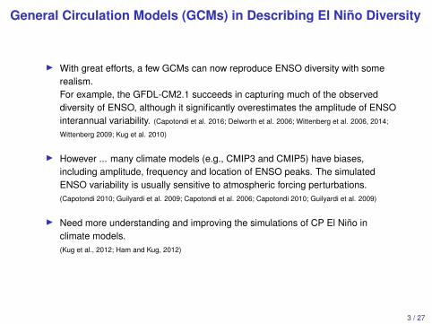
General Circulation Models (GCMs) in Describing El Niño Diversity

I With great efforts, a few GCMs can now reproduce ENSO diversity with somerealism.For example, the GFDL-CM2.1 succeeds in capturing much of the observeddiversity of ENSO, although it significantly overestimates the amplitude of ENSOinterannual variability. (Capotondi et al. 2016; Delworth et al. 2006; Wittenberg et al. 2006, 2014;

Wittenberg 2009; Kug et al. 2010)

I However ... many climate models (e.g., CMIP3 and CMIP5) have biases,including amplitude, frequency and location of ENSO peaks. The simulatedENSO variability is usually sensitive to atmospheric forcing perturbations.(Capotondi 2010; Guilyardi et al. 2009; Capotondi et al. 2006; Capotondi 2010; Guilyardi et al. 2009)

I Need more understanding and improving the simulations of CP El Niño inclimate models.(Kug et al., 2012; Ham and Kug, 2012)

3 / 27

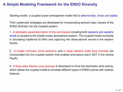
A Simple Modeling Framework for the ENSO Diversity

Starting model: a coupled ocean-atmosphere model that is deterministic, linear and stable.

Then systematic strategies are developed for incorporating several major causes of theENSO diversity into the coupled system:

1. A stochastic parameterization of the wind bursts including both westerly and easterlywinds is coupled to the simple ocean-atmosphere system. The coupled model succeedsin simulating traditional El Niño and capturing the observational record in the easternPacific.

2. A simple nonlinear zonal advection and a mean easterly trade wind anomaly areincorporated into the coupled system that enables anomalous warm SST in the centralPacific.

3. A three-state Markov jump process is developed to drive the stochastic wind activity,which allows the coupled model to simulate different types of ENSO events with realisticfeatures.

4 / 27

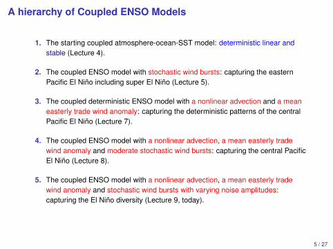
A hierarchy of Coupled ENSO Models

1. The starting coupled atmosphere-ocean-SST model: deterministic linear andstable (Lecture 4).

2. The coupled ENSO model with stochastic wind bursts: capturing the easternPacific El Niño including super El Niño (Lecture 5).

3. The coupled deterministic ENSO model with a nonlinear advection and a meaneasterly trade wind anomaly: capturing the deterministic patterns of the centralPacific El Niño (Lecture 7).

4. The coupled ENSO model with a nonlinear advection, a mean easterly tradewind anomaly and moderate stochastic wind bursts: capturing the central PacificEl Niño (Lecture 8).

5. The coupled ENSO model with a nonlinear advection, a mean easterly tradewind anomaly and stochastic wind bursts with varying noise amplitudes:capturing the El Niño diversity (Lecture 9, today).

5 / 27

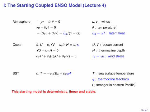
I: The Starting Coupled ENSO Model (Lecture 4)

Atmosphere

Ocean

SST

− yv − ∂xθ = 0

yu − ∂yθ = 0

− (∂x u + ∂y v) = Eq/(1− Q)

∂τU − c1YV + c1∂x H = c1τx

YU + ∂Y H = 0

∂τH + c1(∂x U + ∂Y V ) = 0

∂τT = −c1ζEq + c1ηH

u, v : winds

θ : temperature

Eq = αT : latent heat

U,V : ocean current

H : thermocline depth

τx = γu : wind stress

T : sea surface temperature

η : thermocline feedback

(η stronger in eastern Pacific)

This starting model is deterministic, linear and stable.

6 / 27

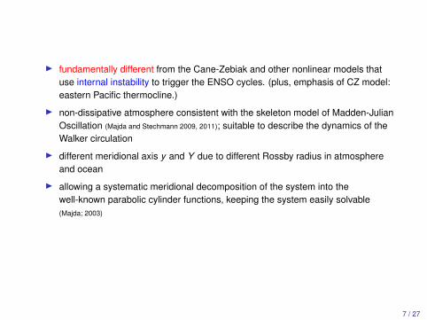
I fundamentally different from the Cane-Zebiak and other nonlinear models thatuse internal instability to trigger the ENSO cycles. (plus, emphasis of CZ model:eastern Pacific thermocline.)

I non-dissipative atmosphere consistent with the skeleton model of Madden-JulianOscillation (Majda and Stechmann 2009, 2011); suitable to describe the dynamics of theWalker circulation

I different meridional axis y and Y due to different Rossby radius in atmosphereand ocean

I allowing a systematic meridional decomposition of the system into thewell-known parabolic cylinder functions, keeping the system easily solvable(Majda; 2003)

7 / 27

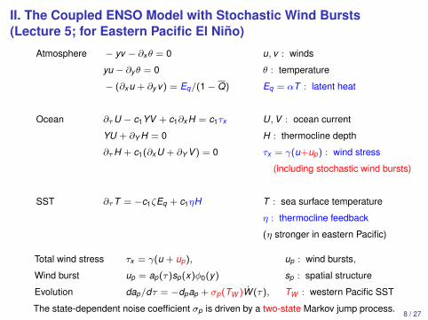
II. The Coupled ENSO Model with Stochastic Wind Bursts(Lecture 5; for Eastern Pacific El Niño)

Atmosphere

Ocean

SST

− yv − ∂xθ = 0

yu − ∂yθ = 0

− (∂x u + ∂y v) = Eq/(1− Q)

∂τU − c1YV + c1∂x H = c1τx

YU + ∂Y H = 0

∂τH + c1(∂x U + ∂Y V ) = 0

∂τT = −c1ζEq + c1ηH

u, v : winds

θ : temperature

Eq = αT : latent heat

U,V : ocean current

H : thermocline depth

τx = γ(u+up) : wind stress

(including stochastic wind bursts)

T : sea surface temperature

η : thermocline feedback

(η stronger in eastern Pacific)

Total wind stress

Wind burst

Evolution

τx = γ(u + up),

up = ap(τ)sp(x)φ0(y)

dap/dτ = −dpap + σp(TW )W (τ),

up : wind bursts,

sp : spatial structure

TW : western Pacific SST

The state-dependent noise coefficient σp is driven by a two-state Markov jump process.8 / 27

Stochastic Wind Bursts: in western Pacific depending on warm pool SST

Total wind stress

Wind burst

Evolution

τx = γ(u + up),

up = ap(τ)sp(x)φ0(y)

dap/dτ = −dpap + σp(TW )W (τ),

up : wind bursts,

sp : spatial structure

TW : western Pacific SST

Markov Jump Process: stochastic dependency on warm pool SST

Markov States

States Switch

σp(TW ) =

{σp0 : quiescent

σp1 : active

P(quiescent→ active at t + ∆t) = r01∆t + o(∆t)

P(active→ quiescent at t + ∆t) = r10∆t + o(∆t)

Fundamentally different from Jin et al., 2007 that relies on the eastern Pacific SSTand D. Chen et al., 2015 that requires ad hoc prescription of wind burst thresholds. 9 / 27

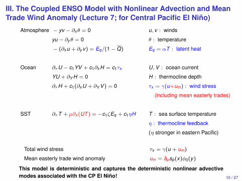
III. The Coupled ENSO Model with Nonlinear Advection and MeanTrade Wind Anomaly (Lecture 7; for Central Pacific El Niño)

Atmosphere

Ocean

SST

− yv − ∂xθ = 0

yu − ∂yθ = 0

− (∂x u + ∂y v) = Eq/(1− Q)

∂τU − c1YV + c1∂x H = c1τx

YU + ∂Y H = 0

∂τH + c1(∂x U + ∂Y V ) = 0

∂τT + µ∂x (UT ) = −c1ζEq + c1ηH

u, v : winds

θ : temperature

Eq = αT : latent heat

U,V : ocean current

H : thermocline depth

τx = γ(u+um) : wind stress

(including mean easterly trades)

T : sea surface temperature

η : thermocline feedback

(η stronger in eastern Pacific)

Total wind stress

Mean easterly trade wind anomaly

τx = γ(u + um)

um = apsp(x)φ0(y)

This model is deterministic and captures the deterministic nonlinear advectivemodes associated with the CP El Niño! 10 / 27

IV. The Coupled ENSO Model with Nonlinear Advection, StochasticWind Bursts, Mean Trade Wind Anomaly and Small to ModerateStochastic Wind Bursts (Lecture 8; for Central Pacific El Niño)

Atmosphere

Ocean

SST

− yv − ∂xθ = 0

yu − ∂yθ = 0

− (∂x u + ∂y v) = Eq/(1− Q)

∂τU − c1YV + c1∂x H = c1τx

YU + ∂Y H = 0

∂τH + c1(∂x U + ∂Y V ) = 0

∂τT + µ∂x (UT ) = −c1ζEq + c1ηH

u, v : winds

θ : temperature

Eq = αT : latent heat

U,V : ocean current

H : thermocline depth

τx = γ(u+up) : wind stress

(including wind bursts + trades)

T : sea surface temperature

η : thermocline feedback

(η stronger in eastern Pacific)

Total wind stress

Wind burst + mean trade wind anomaly

Evolution

τx = γ(u + up)

up = ap(τ)sp(x)φ0(y)

dap/dτ = −dp(ap−ap) + σp(TW )W (τ)

The trade wind ap and the noise coefficient σp are driven by a two-state Markov jumpprocess.

11 / 27

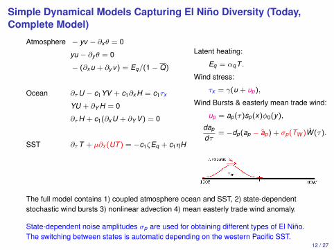
Simple Dynamical Models Capturing El Niño Diversity (Today,Complete Model)

Atmosphere

Ocean

SST

− yv − ∂xθ = 0

yu − ∂yθ = 0

− (∂x u + ∂y v) = Eq/(1− Q)

∂τU − c1YV + c1∂x H = c1τx

YU + ∂Y H = 0

∂τH + c1(∂x U + ∂Y V ) = 0

∂τT + µ∂x (UT ) = −c1ζEq + c1ηH

Latent heating:

Eq = αqT .

Wind stress:

τx = γ(u + up),

Wind Bursts & easterly mean trade wind:

up = ap(τ)sp(x)φ0(y),

dap

dτ= −dp(ap − ap) + σp(TW )W (τ).

The full model contains 1) coupled atmosphere ocean and SST, 2) state-dependentstochastic wind bursts 3) nonlinear advection 4) mean easterly trade wind anomaly.

State-dependent noise amplitudes σp are used for obtaining different types of El Niño.The switching between states is automatic depending on the western Pacific SST.

12 / 27

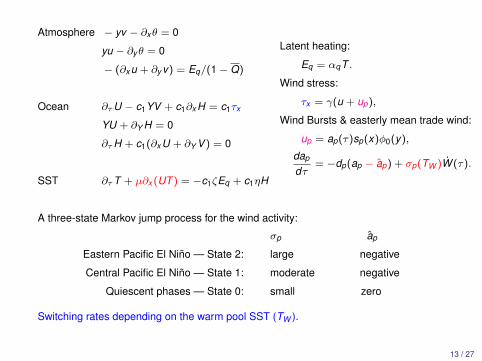
Atmosphere

Ocean

SST

− yv − ∂xθ = 0

yu − ∂yθ = 0

− (∂x u + ∂y v) = Eq/(1− Q)

∂τU − c1YV + c1∂x H = c1τx

YU + ∂Y H = 0

∂τH + c1(∂x U + ∂Y V ) = 0

∂τT + µ∂x (UT ) = −c1ζEq + c1ηH

Latent heating:

Eq = αqT .

Wind stress:

τx = γ(u + up),

Wind Bursts & easterly mean trade wind:

up = ap(τ)sp(x)φ0(y),

dap

dτ= −dp(ap − ap) + σp(TW )W (τ).

A three-state Markov jump process for the wind activity:

σp ap

Eastern Pacific El Niño — State 2: large negative

Central Pacific El Niño — State 1: moderate negative

Quiescent phases — State 0: small zero

Switching rates depending on the warm pool SST (TW ).

13 / 27

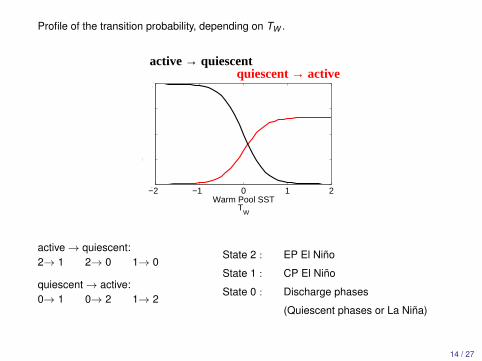
Profile of the transition probability, depending on TW .

−2 −1 0 1 20

0.5

1

1.5

2

Warm Pool SSTT

W

active → quiescentquiescent → active

active→ quiescent:2→ 1 2→ 0 1→ 0

quiescent→ active:0→ 1 0→ 2 1→ 2

State 2 : EP El Niño

State 1 : CP El Niño

State 0 : Discharge phases

(Quiescent phases or La Niña)

14 / 27

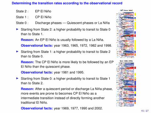
Determining the transition rates according to the observational record

State 2 : EP El Niño

State 1 : CP El Niño

State 0 : Discharge phases — Quiescent phases or La Niña

I Starting from State 2: a higher probability to transit to State 0than to State 1.

Reason: An EP El Niño is usually followed by a La Niña.

Observational facts: year 1963, 1965, 1972, 1982 and 1998.

I Starting from State 1: a higher probability to transit to State 2than to State 0.

Reason: The CP El Niño is more likely to be followed by an EPEl Niño than the quiescent phase.

Observational facts: year 1981 and 1995.

I Starting from State 0: a higher probability to transit to State 1than to State 2.

Reason: After a quiescent period or discharge La Niña phase,more events are prone to becomes CP El Niño as aintermediate transition instead of directly forming anothertraditional El Niño.

Observational facts: year 1969, 1977, 1990 and 2002.15 / 27

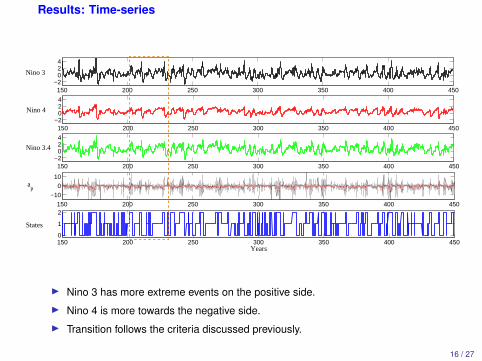
Results: Time-series

150 200 250 300 350 400 450−2

024

Nino 3

150 200 250 300 350 400 450−2

024

Nino 4

150 200 250 300 350 400 450−2

024

Nino 3.4

150 200 250 300 350 400 450

−10

0

10a

p

150 200 250 300 350 400 4500

1

2

States

Years

I Nino 3 has more extreme events on the positive side.

I Nino 4 is more towards the negative side.

I Transition follows the criteria discussed previously.

16 / 27

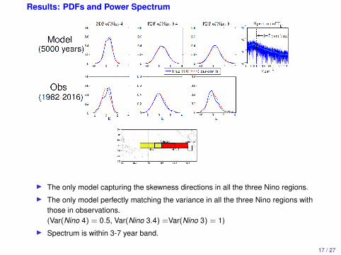
Results: PDFs and Power Spectrum

I The only model capturing the skewness directions in all the three Nino regions.I The only model perfectly matching the variance in all the three Nino regions with

those in observations.(Var(Nino 4) = 0.5, Var(Nino 3.4) =Var(Nino 3) = 1)

I Spectrum is within 3-7 year band.

17 / 27

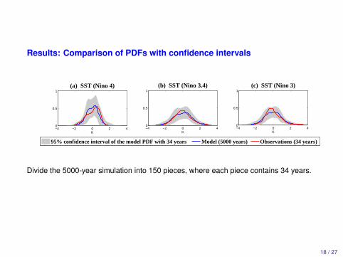
Results: Comparison of PDFs with confidence intervals

−4 −2 0 2 40

0.5

1(a) SST (Nino 4)

K

95% confidence interval of the model PDF with 34 years Model (5000 years) Observations (34 years)

−4 −2 0 2 40

0.5

1(b) SST (Nino 3.4)

K−4 −2 0 2 40

0.5

1(c) SST (Nino 3)

K

Divide the 5000-year simulation into 150 pieces, where each piece contains 34 years.

18 / 27

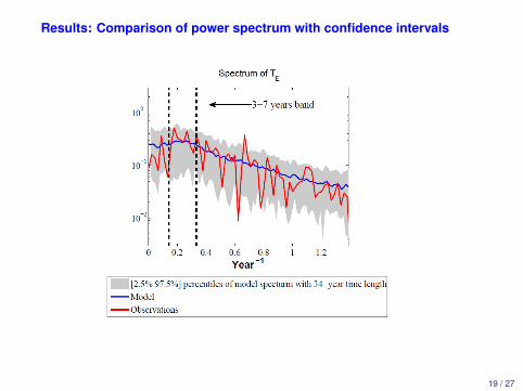
Results: Comparison of power spectrum with confidence intervals

19 / 27

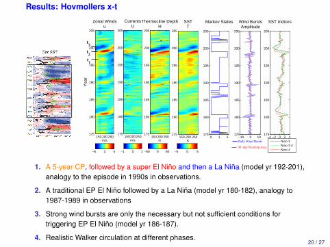
Results: Hovmollers x-t

0 1 2175

180

185

190

195

200

205

Markov States

m/s

CurrentsU

150200250175

180

185

190

195

200

205

−1 0 1

m

Thermocline DepthH

150 200 250175

180

185

190

195

200

205

−50 0 50

K

SSTT

150 200 250175

180

185

190

195

200

205

−5 0 5

−10 0 10175

180

185

190

195

200

205

Wind BurstsAmplitude

m/s

Yea

r

Zonal Windsu

150 200 250175

180

185

190

195

200

205

−5 0 5

−4 −2 0 2 4175

180

185

190

195

200

205

SST Indices

Nino 3Nino 3.4Nino 4

t3

t2

t1

Daily Wind Bursts

90−day Running Avg

1. A 5-year CP, followed by a super El Niño and then a La Niña (model yr 192-201),analogy to the episode in 1990s in observations.

2. A traditional EP El Niño followed by a La Niña (model yr 180-182), analogy to1987-1989 in observations

3. Strong wind bursts are only the necessary but not sufficient conditions fortriggering EP El Niño (model yr 186-187).

4. Realistic Walker circulation at different phases.20 / 27

Results: Hovmollers x-t

0 1 2175

180

185

190

195

200

205

Markov States

m/s

CurrentsU

150200250175

180

185

190

195

200

205

−1 0 1

m

Thermocline DepthH

150 200 250175

180

185

190

195

200

205

−50 0 50

K

SSTT

150 200 250175

180

185

190

195

200

205

−5 0 5

−10 0 10175

180

185

190

195

200

205

Wind BurstsAmplitude

m/s

Yea

r

Zonal Windsu

150 200 250175

180

185

190

195

200

205

−5 0 5

−4 −2 0 2 4175

180

185

190

195

200

205

SST Indices

Nino 3Nino 3.4Nino 4

t3

t2

t1

Daily Wind Bursts

90−day Running Avg

21 / 27

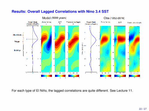
Results: Overall Lagged Correlations with Nino 3.4 SST

For each type of El Niño, the lagged correlations are quite different. See Lecture 11.

22 / 27

Results: Sensitivity tests

75% 85% 95% 105% 115% 125%0

0.2

0.4

0.6

0.8

1

1.2(a) ν21/ν

∗

21 and ν20/ν∗

20

T−3

T−4

T−3.4

75% 85% 95% 105% 115% 125%0

0.2

0.4

0.6

0.8

1

1.2(b) ν10/ν

∗

10

75% 85% 95% 105% 115% 125%0

0.2

0.4

0.6

0.8

1

(c) ν12/ν∗

12

75% 85% 95% 105% 115% 125%0

0.2

0.4

0.6

0.8

1

(d) ν01/ν∗

01 and ν02/ν∗

02

75% 85% 95% 105% 115% 125%0

0.2

0.4

0.6

0.8

1

(e) ν21/ν∗

21 and ν∗

20/ν20

75% 85% 95% 105% 115% 125%0

0.2

0.4

0.6

0.8

1

(f) ν01/ν∗

01 and ν∗

02/ν02

Variance

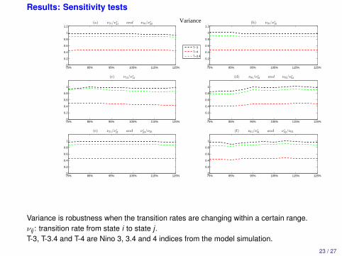
Variance is robustness when the transition rates are changing within a certain range.νij : transition rate from state i to state j .T-3, T-3.4 and T-4 are Nino 3, 3.4 and 4 indices from the model simulation.

23 / 27

Results: Sensitivity tests

75% 85% 95% 105% 115% 125%

−0.4

−0.2

0

0.2

0.4

0.6(a) ν21/ν

∗

21 and ν20/ν∗

20

T−3

T−4

T−3.4

75% 85% 95% 105% 115% 125%

−0.4

−0.2

0

0.2

0.4

0.6(b) ν10/ν

∗

10

75% 85% 95% 105% 115% 125%

−0.4

−0.2

0

0.2

0.4

0.6(c) ν12/ν

∗

12

75% 85% 95% 105% 115% 125%

−0.4

−0.2

0

0.2

0.4

0.6(d) ν01/ν

∗

01 and ν02/ν∗

02

75% 85% 95% 105% 115% 125%

−0.4

−0.2

0

0.2

0.4

0.6(e) ν21/ν

∗

21 and ν∗

20/ν20

75% 85% 95% 105% 115% 125%

−0.4

−0.2

0

0.2

0.4

0.6(f) ν01/ν

∗

01 and ν∗

02/ν02

Skewness

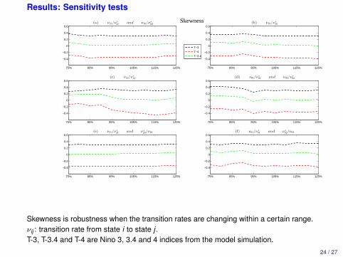
Skewness is robustness when the transition rates are changing within a certain range.νij : transition rate from state i to state j .T-3, T-3.4 and T-4 are Nino 3, 3.4 and 4 indices from the model simulation.

24 / 27

Results: Sensitivity tests

75% 85% 95% 105% 115% 125%2.5

3

3.5

4

4.5(a) ν21/ν

∗

21 and ν20/ν∗

20

T−3

T−4

T−3.4

75% 85% 95% 105% 115% 125%2.5

3

3.5

4

4.5(b) ν10/ν

∗

10

75% 85% 95% 105% 115% 125%2.5

3

3.5

4

4.5(c) ν12/ν

∗

12

75% 85% 95% 105% 115% 125%2.5

3

3.5

4

4.5(d) ν01/ν

∗

01 and ν02/ν∗

02

75% 85% 95% 105% 115% 125%2.5

3

3.5

4

4.5(e) ν21/ν

∗

21 and ν∗

20/ν20

75% 85% 95% 105% 115% 125%2.5

3

3.5

4

4.5(f) ν01/ν

∗

01 and ν∗

02/ν02

Kurtosis

Kurtosis is robustness when the transition rates are changing within a certain range.νij : transition rate from state i to state j .T-3, T-3.4 and T-4 are Nino 3, 3.4 and 4 indices from the model simulation.

25 / 27

Summary

1. Review of the model studied in previous lectures.

2. A three-state Markov jump process is developed to drive the stochastic windactivity, which allows the coupled model to simulate different types of ENSOevents with realistic features.

3. Model simulations: capturing the El Niño diversity and statistical features indifferent Nino regions.

Next two lectures:Comparison of model mechanisms and more statistical features with observations innature.

26 / 27

Thank you

27 / 27