pdfs.semanticscholar.org€¦ · contents 1 introduction 1 2 simulation framework 3 2.1 hybrid...
TRANSCRIPT
eeh power systemslaboratory
Comparison of Phasor Dynamics Approach to different ModelingTechniques in a common Simulation Framework
Version 1.0
Turhan Demiray
Internal ReportZurich, March 2006

white

Contents
1 Introduction 1
2 Simulation Framework 3
2.1 Hybrid System Representation . . . . . . . . . . . . . . . . . . . . . . . . . . . . . . 3
2.2 Implementation of Simulation Kernel . . . . . . . . . . . . . . . . . . . . . . . . . . . 6
2.2.1 Initialization . . . . . . . . . . . . . . . . . . . . . . . . . . . . . . . . . . . . 8
2.2.2 Calculation of Continuous Trajectory . . . . . . . . . . . . . . . . . . . . . . 9
2.2.3 Event Handling and Consistent Reinitialization . . . . . . . . . . . . . . . . . 11
2.3 Automatic Code Generator . . . . . . . . . . . . . . . . . . . . . . . . . . . . . . . . 13
2.4 Summary . . . . . . . . . . . . . . . . . . . . . . . . . . . . . . . . . . . . . . . . . . 17
3 Modeling Techniques 18
3.1 Models in Three-Phase (ABC) Reference Frame . . . . . . . . . . . . . . . . . . . . . 20
3.2 Models in DQ0 Reference Frame . . . . . . . . . . . . . . . . . . . . . . . . . . . . . 21
3.3 Dynamic Phasor Models . . . . . . . . . . . . . . . . . . . . . . . . . . . . . . . . . . 23
3.4 Application Example - TCSC . . . . . . . . . . . . . . . . . . . . . . . . . . . . . . . 27
3.5 Modeled Components . . . . . . . . . . . . . . . . . . . . . . . . . . . . . . . . . . . 33
3.6 Reduced Order Models . . . . . . . . . . . . . . . . . . . . . . . . . . . . . . . . . . 35
3.7 Summary . . . . . . . . . . . . . . . . . . . . . . . . . . . . . . . . . . . . . . . . . . 38
4 Results 39
4.1 Simulations with Detailed Models . . . . . . . . . . . . . . . . . . . . . . . . . . . . . 39
4.1.1 SMIB system . . . . . . . . . . . . . . . . . . . . . . . . . . . . . . . . . . . 39
4.1.2 Two Area System Without TCSC . . . . . . . . . . . . . . . . . . . . . . . . 41
4.1.3 Two Area System With TCSC . . . . . . . . . . . . . . . . . . . . . . . . . . 42
4.2 Simulations with Reduced Order Models . . . . . . . . . . . . . . . . . . . . . . . . . 43
4.3 Summary . . . . . . . . . . . . . . . . . . . . . . . . . . . . . . . . . . . . . . . . . . 44
5 Appendix 45
5.1 Fourier coefficients in real form . . . . . . . . . . . . . . . . . . . . . . . . . . . . . . 45
5.2 TCSC - Harmonic Distortion Factor of Capacitor Voltage . . . . . . . . . . . . . . . . 46

List of Figures
1.1 Aim of the project . . . . . . . . . . . . . . . . . . . . . . . . . . . . . . . . . . . . . 2
2.1 Directed graph view of a hybrid system . . . . . . . . . . . . . . . . . . . . . . . . . . 3
2.2 Sample trajectory of a hybrid system . . . . . . . . . . . . . . . . . . . . . . . . . . . 5
2.3 Simple Example of a system in DSAR structure . . . . . . . . . . . . . . . . . . . . . 6
2.4 Illustration of the overall System Function Structure . . . . . . . . . . . . . . . . . . . 8
2.5 Flow chart during continuous conditions . . . . . . . . . . . . . . . . . . . . . . . . . 11
2.6 Trajectory of an event variable ye with event occurring at te . . . . . . . . . . . . . . 12
2.7 Flow chart of the overall simulation . . . . . . . . . . . . . . . . . . . . . . . . . . . . 13
2.8 Model - Simulation Kernel interface . . . . . . . . . . . . . . . . . . . . . . . . . . . 14
2.9 Example RC-circuit with corresponding MDF . . . . . . . . . . . . . . . . . . . . . . 15
2.10 Simulation results of the RC-circuit . . . . . . . . . . . . . . . . . . . . . . . . . . . . 16
3.1 Modeling Techniques . . . . . . . . . . . . . . . . . . . . . . . . . . . . . . . . . . . 19
3.2 Circuit diagram of Π transmission line model . . . . . . . . . . . . . . . . . . . . . . 19
3.3 Unbalanced set of phasors as a sum of balanced phasors . . . . . . . . . . . . . . . . 20
3.4 Circuit diagram of TCSC . . . . . . . . . . . . . . . . . . . . . . . . . . . . . . . . . 27
3.5 (a) Steady-state and (b) Transient waveforms of il(t), v(t), i(t) . . . . . . . . . . . . . 27
3.6 Harmonic Distortion . . . . . . . . . . . . . . . . . . . . . . . . . . . . . . . . . . . . 30
3.7 Test case for TCSC . . . . . . . . . . . . . . . . . . . . . . . . . . . . . . . . . . . . 31
3.8 Capacitor voltage of the TCSC (a) whole simulation interval (b) zoomed section . . . 32
3.9 Circuit diagram one phase to ground fault . . . . . . . . . . . . . . . . . . . . . . . . 33
3.10 Fault representation in transient stability programs . . . . . . . . . . . . . . . . . . . 36
4.1 Single-line diagram of SMIB system . . . . . . . . . . . . . . . . . . . . . . . . . . . 39
4.2 Electrical Torque of GEN (a) whole simulation (b) during fault (c) after fault . . . . . 40
4.3 Single-line diagram of Two Area System without TCSC . . . . . . . . . . . . . . . . . 41
4.4 Electrical Torque of GEN1 (a) whole simulation (b) during fault (c) after fault . . . . 41
4.5 Electrical Torque of GEN1 (a) whole simulation (b) zoomed section . . . . . . . . . . 42
4.6 Electrical Torque of GEN during fault . . . . . . . . . . . . . . . . . . . . . . . . . . 43
4.7 Negative sequence Electrical Torque of GEN during fault . . . . . . . . . . . . . . . . 43

List of Tables
2.1 Ψ , Ψf and Ψh of implemented integration methods . . . . . . . . . . . . . . . . . . 10
2.2 RC-Circuit equations in DSAR structure . . . . . . . . . . . . . . . . . . . . . . . . . 15
3.1 DQ0 transformations of sequence components of iabc . . . . . . . . . . . . . . . . . . 22
3.2 Steady-state capacitor voltage vs(t) over a period . . . . . . . . . . . . . . . . . . . 29
3.3 Sequence of events . . . . . . . . . . . . . . . . . . . . . . . . . . . . . . . . . . . . 32
4.1 Simulation times for SMIB . . . . . . . . . . . . . . . . . . . . . . . . . . . . . . . . 40
4.2 Simulation times for Two Area System . . . . . . . . . . . . . . . . . . . . . . . . . 42

white

Chapter 1
Introduction
The dynamic behavior of physical systems are most often studied with appropriate simulation programs.The implementation of such simulation programs undergoes following stages.
Mathematical Representation: The dynamic behavior of physical systems (e.g. Power sys-tem) obey physical laws. Mathematically, this physical behavior is represented as a set of equations,which capture all the important characteristics of such systems. For example in the case of powersystems, there are components, such as synchronous machines, where dynamic behavior is reflectedby differential-algebraic equations, with rotor angles (δ), fluxes (Ψ) as continuous dynamic states anddq-currents (Id, Iq) as algebraic states. Besides, there are also components, which have discrete charac-teristics, such as tap changing transformers and relays. As the whole system is interconnected, there isa permanent interaction between continuous and discrete dynamics. The mathematical representationof the models should capture both continuous and discrete nature of the components.
Another important issue in the implementation phase is also choice of causal modeling or non-causalmodeling as model representation.
Causal Modeling - Input/Output Representation: The model behavior is described by a rigidinput/output relation (e.g. y = g(u)). Causal modeling is like a method computing output values byoperating on input values. Some variables of the model are defined as inputs and some as outputs.The output (y) can be calculated if the input (u) is defined. Building systems by connecting suchcausal models means actually, the output of one model is used as an input to another model. Forexample for a resistor the causal way of modeling would be, V = R · I, where we defined current Ias an input (u), and the voltage across the resistor V as an output (y). For example, the MATLABbased simulation program SIMULINK uses the causal modeling approach.
Non-causal Modeling - Modular Representation: The major difference to causal modeling isthat in this representation, there is no distinction between input and output variables. In non-causalmodeling, variables are involved in equations that must be satisfied, to reflect the components behavior.For a resistor, the behavior is fully defined by the equation V −R ·I = 0, which is an algebraic equation.Building systems by connecting non-causal models clearly induces some additional constraints on thevalue that a variable at both terminals can take. The behavior of such an interconnected systemis defined in terms of the signals that satisfy both the modules behaviors and the interconnectionconstraints induced by the interconnection architecture. One of the advantages of non-causal modelingis, that it allows to use directly the models equations. For example, MODELICA uses the non-causalmodeling approach.
Modeling Technique: Sometimes, important characteristics of the physical system can lead tosome simplifications or useful approximations of the model equations, which still reflect the dynamicbehavior appropriately and make simulations more efficient. For example in the case of power systemssuch characteristics are:
• Periodicity of the balanced three-phase quantities.
1

2
• Periodical switchings of FACTS devices.
• Different time scales in the dynamic behavior (fast or slow phenomena).
Numerical Methods: The previous two points were focused on the analytical aspects of the sys-tem modeling. Another important issue in simulation of physical systems is also the numerical methodsapplied to calculate the continuous trajectories of system variables. There are various numerical inte-gration methods used for this purpose. The main differences of these methods are in
• Numerical Accuracy.
• Numerical Efficiency.
• Numerical Stability.
It is also important to mention, that the time-scale characteristics of the physical system plays arelevant role in the selection of suitable numerical integration method.
Here in this report, our focus will be on the first two points described above. Firstly we will choosean appropriate mathematical representation for power system components, which captures all theimportant characteristics, and build a simulation framework based upon this representation. Secondlywe will investigate different modeling techniques applied in power systems area and compare theiraccuracy and efficiency in the implemented simulation framework.
Differently
Modeled Components
Comparison of
accuracy
Same
Simulation framework
Comparison of
efficiency
Figure 1.1: Aim of the project

Chapter 2
Simulation Framework
Our focus in this chapter is on the implemented mathematical representation proposed in [1] and [2],which captures all the important aspects of a power system. Based on this mathematical representation,we have implemented a non-causal simulation framework in MATLAB. Firstly, we will give a detailedinsight into the proposed mathematical representation and describe in detail the implemented simulationframework. After that, our focus will be on some implemented tools, which ease the model developmentfor the users.
2.1 Hybrid System Representation
Hybrid Systems are systems, where the system behavior is governed by both discrete and continuousstates. There is such a strong coupling between these discrete and continuous behavior of the system,so that they must be analyzed simultaneously. Generally, a hybrid system can be thought as a directedgraph as illustrated in figure 2.1, where the nodes describe the system behavior at a given mode andthe edges show the conditions and directions of the transition from one system mode to another. If
System at Mode 1
System at Mode 2
System at Mode 3System at Mode 4
y1 > 0
y2 < 0 ∨ y4 < 0
y3 == 0
y4 > 0
y5 < 0
Figure 2.1: Directed graph view of a hybrid system
one transition condition is fulfilled, the system jumps from one mode to an other and remains there,till another transition condition is fulfilled, which takes the system to one other mode. In physicalsystems, the continuous system behavior at different modes can be described by Ordinary DifferentialEquations (ODEs), Differential-Algebraic Equations (DAEs) or Partial Differential Equations (PDEs)
3
2.1. Hybrid System Representation 4
depending on system characteristics.
Power systems are an important class of hybrid systems, as they exhibit discrete and continuousstates. The continuous-time dynamic behavior of the power system is driven by components suchas synchronous machines with continuous dynamic states x like rotor angle δ and rotor circuit fluxesΨfd, Ψ1d, Ψ1q, Ψ2q or loads with algebraic states y like voltage magnitudes |V | and voltage angles θ.The discrete behavior of the power system is governed by components such as tap changing transformerswith discrete dynamic state z like tap position n. As the entire system consists of such interconnectedcomponents, there is a permanent interaction between these two aspects of system behavior, whichmakes the power system an important class of hybrid systems. The continuous-time dynamic behaviorof the power system at a mode can be described by DAEs. The discrete events or switching actionsinherent in power systems, force the system to jump to another system mode as illustrated in figure2.1, where the continuous behavior of the system is described by another set of DAEs. This jump tonew set of DAEs can be caused due to a change in a discrete state variable e.g. tap position of a tapchanging transformer.
As proposed in [1] and [2], such a hybrid system behavior can be modeled by a set of Differential,Switched Algebraic and State Reset equations (DSAR) as given in equations (2.1) - (2.6).
x = f(x, y, z, λ) (2.1)
z = 0 (2.2)
λ = 0 (2.3)
0 = g(0)(x, y) (2.4)
0 =
{g(i−)(x, y, z, λ) yd,i < 0g(i+)(x, y, z, λ) yd,i > 0
i = 1,......,d (2.5)
z+ = hj(x−, y−, z−, λ) ye,j = 0 j ∈ {1, ...., e} (2.6)
It can easily be seen, that (2.1) describes the differential equations, (2.4) and (2.5) the so calledswitched algebraic equations and (2.6) the state reset equations, where
• x are continuous dynamic states
• z are discrete dynamic states
• y are algebraic states
• λ are parameters
The superscript − stands for pre-event values and + for post event values. At the beginning, thesystem behavior is described by the DAE given in (2.1) and (2.4). A transition to another set of DAEtakes place if the corresponding transition condition is fulfilled. Such transition conditions are checkedby means of so called event variables yd and ye. The yd determine the switching events and ye statereset events. An event is triggered by an element of yd changing sign and/or an element of ye passingthrough zero. By switching events, which are caused by yd sign changes, the functional description ofthe system is changed from g(i−)(x, y) to g(i+)(x, y). Generally, there are two kind of events, whichcan occur, either time events or state events. The time events occur always at a specified future time.The fault time of a short circuit (e.g. at 0.1 sec) is a time driven event. The state events occur onlythen if some conditions on continuous states are satisfied, thus the time, when the event occurs, isnot known before. For example, the tripping of a relay dependent on the current through it, is such astate event.
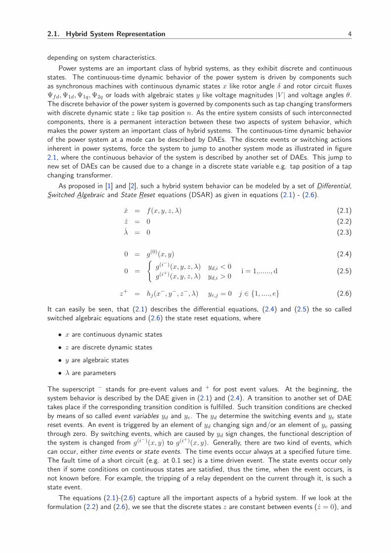
The equations (2.1)-(2.6) capture all the important aspects of a hybrid system. If we look at theformulation (2.2) and (2.6), we see that the discrete states z are constant between events (z = 0), and
2.1. Hybrid System Representation 5
at state reset events caused by ye, the values of the discrete states change according to the functionhj . At state reset events, the values of dynamic states x are continuous, which is reasonable in physicalsystems. Actually if we look at the (2.3) the parameters λ are always constant. The reason to includethem in this formulation as dynamic states is to calculate some sensitivities.
x = f(x, y, z, λ)
0 = g(0)(x, y, z, λ)
x = f(x, y, z, λ)
0 = g(1)(x, y, z, λ)
x = f(x, y, z, λ)
0 = g(2)(x, y, z, λ)
z+ = h1(x−, y−, z−, λ) z+ = h2(x
−, y−, z−, λ)
zxy
0.11 0.15 0.19 0.23
-2.0
-1.0
0.0
1.0
2.0
3.0
4.0
5.0
t1 t2
Figure 2.2: Sample trajectory of a hybrid system
Figure 2.2 illustrates the evolution some different system variable trajectories. Between t = 0and t = t1, the system behavior is governed by the continuous DAE x = f(x, y, z, λ) and 0 =g(0)(x, y, z, λ). In this interval the continuous dynamic states x and algebraic states y evolve overtime,where as the discrete dynamic states z remain constant. At time t1 an event occurs and the systemjumps to another mode as shown in figure 2.1. After such a transition, the system must be reinitializedconsistently. At the event point, the post-event values of the system variables (x+, y+, z+) mustbe calculated dependent on the pre-event values (x−, y−, z−) with the state-reset function (h) andmode switch function (g(i+)). As mentioned before, the post-event values of the continuous dynamicstates are continuous (x+ = x−). The corresponding post-event values of discrete dynamic statesz are calculated according to z+ = h1(x−, y−, z−, λ). After z+ are calculated, post-event values ofalgebraic variables y+ are calculated by solving the nonlinear equation 0 = g(1)(x+, y+, z+, λ) at t = t1.After post-event values and are determined, they serve as initial conditions for the new continuoussection. The system behavior in this section is governed by the equations and x = f(x, y, z, λ) and0 = g(1)(x, y, z, λ). This continues till another event forces the system to switch to another mode andsame reinitialization procedures are applied.
Even though the name of this hybrid system representation, namely ”Differential Switched-Algebraic State-Reset Equations”, relates the discrete nature of the problem only to algebraic equa-tions, there is a hidden ”Switched Ordinary Differential Equation” characteristic in the formulation.Generally the DAEs can be interpreted as dynamic systems defined by x = f(x, y, λ) which move onlyover the constraint manifold defined by g(x, y, λ) = 0. However in some cases, it is possible to representthe algebraic variables y as functions of continuous dynamic variables x. In other words, at any localpoint, say x∗, y∗, the implicit function theorem ensures that there exists a function ψ(x, λ) defined on

2.2. Implementation of Simulation Kernel 6
a neighborhood of x∗ with y∗ = ψ(x∗, λ) and that satisfies g(x∗, ψ(x∗, λ)) = 0. It follows, that thetrajectories of the DAE are locally defined by the ODE x = f(x, ψ(x, λ), λ). Such a representation isonly possible, if the jacobian ∂g/∂y is nonsingular. This means, in the hybrid system representationused here, the algebraic equations g can be indexed with d and z, as different d and different discretestates z mean different constraint manifolds with g(d,z). The implicit function theorem allows now todefine y = ψ(d,z)(x, λ) locally and thus the equation (2.1) becomes x = f(d,z)(x, λ), which can beinterpreted as a hybrid dynamical system model.
2.2 Implementation of Simulation Kernel
The DSAR structure is actually a modular representation of a model, where the behavior of the model isdescribed by writing the equations in the proposed form given in (2.1)-(2.6). As there is no distinctionbetween input and output variables, this representation of the models in the DSAR structure is verysuitable for a non-causal modeling. There are many advantages of non-causal modeling. It frees themodeler from the need of converting the model equations to an explicit ODE with an input/outputrelation. A non-causal model is an implicit system of differential and algebraic equations. Non-causalmodeling also supports component hierarchies, allows the reuse of modeling knowledge in an object-oriented manner, which is the state of the art in today’s programming world.
x = f(x, y, z, λ)z = 0
0 = g(0)(x, y, z, λ)
0 =
{g(i−)(x, y, z, λ)
g(i+)(x, y, z, λ)
yd,i > 0yd,i < 0
}
z+ = hj(x−, y−, z−λ) ye,j=0
DSAR structure
Model1 Model2
Model3
g1(y1,1, y1,2) = 0 g2(y2,1, y2,2) = 0
g3(y3,1, y3,2) = 0
y1,1 y1,2 y2,1 y2,2
y3,1 y3,2
y1,1 = y3,1
y1,2 = y2,1
y2,2 = y3,2
Figure 2.3: Simple Example of a system in DSAR structure
An overall system consists of many subsystems connected with interface variables together, wherethe subsystem may also be composed of different models grouped together. The behavior of suchan interconnected system is defined in terms of the signals that satisfy both the modules behaviors(in DSAR structure) and the interconnection constraints induced by the interconnection architecture,which is a set of simple linear algebraic equations c(y) = 0 such as (yj,n = yk,m) → (yj,n − yk,m = 0).c(y) has the general structure of
∑ck · yi,j , where ck can only take values ±1. This is illustrated in
figure 2.3. We have a system consisting of three models where the corresponding model describingfunctions are given in the proposed DSAR structure. To simplify matters, we assume here all models

2.2. Implementation of Simulation Kernel 7
having two algebraic states and the model describing equations g1, g2 and g3 , which are pure algebraic.Besides model equations, we have also three connection equations, which link interface variables ofdifferent models together. The 6 unknown algebraic variables must satisfy the three model equationsand three connection equations.
g1(y1,1, y1,2) = 0g2(y2,1, y2,2) = 0g3(y3,1, y3,2) = 0
y1,1 − y3,1 = 0y1,2 − y2,1 = 0y2,2 − y3,2 = 0
Oversimplifyingly we can say, we have system with 6 unknowns and 6 equations, which is a necessarycondition for the solvability of the system.
If we look at the general case, a system consisting of m models can be described between eventswith a continuous differential-algebraic equation system given as
xi = fi(xi, yi)0 = gi(xi, yi)0 = c(y1, ...., ym)
where
• i ∈ {1....m}• fi and gi are DAEs of the ith model in the current continuous region.
• xi is a set of continuous dynamic states of ith model.
• yi is a set of algebraic states of ith model.
• c(y1, ...., ym) is the linear algebraic connection equation, which defines the topology.
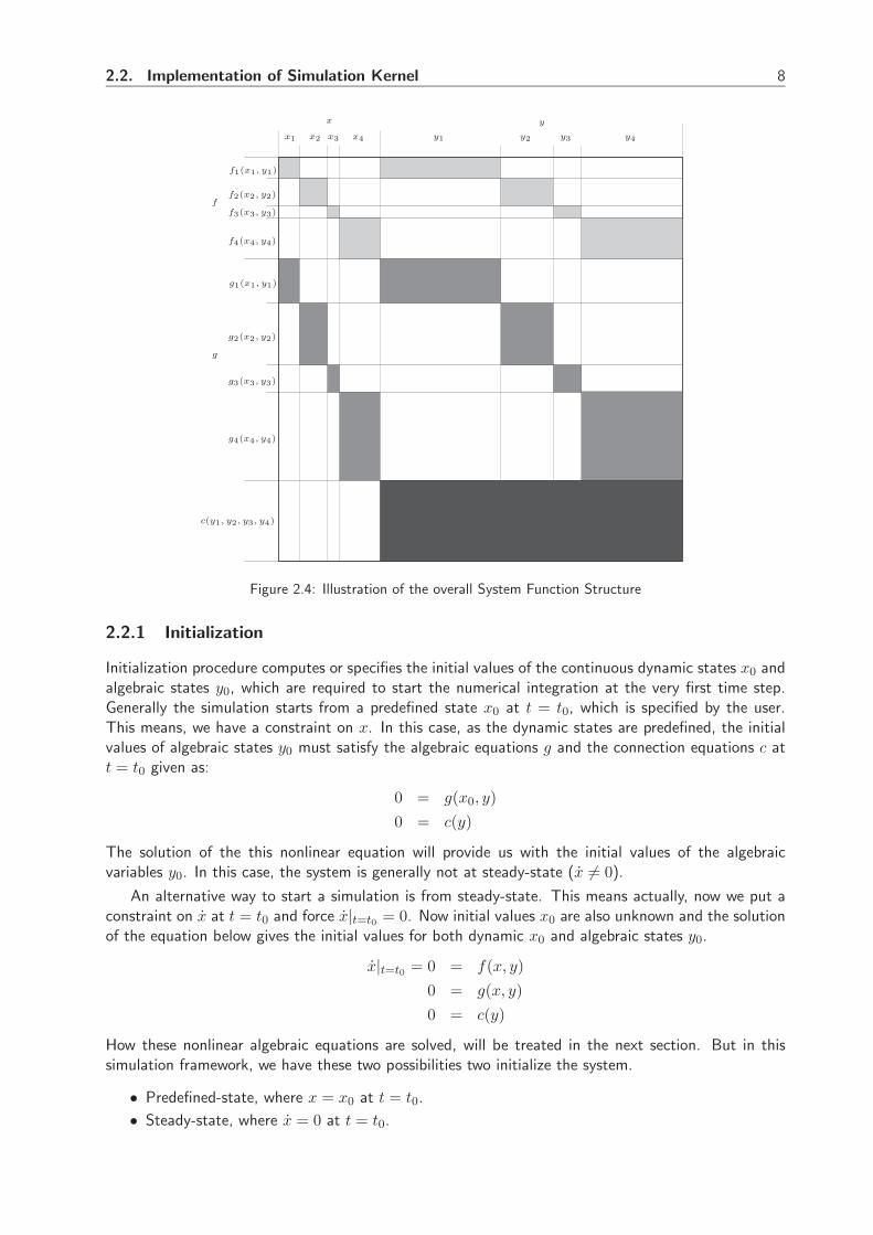
Here, we omitted the z and λ dependence as they are constant between events. The structure of such asystem can be illustrated in a two dimensional array as shown in figure 2.4. The horizontal axis containsall the continuous dynamic states x and algebraic states y. States belonging to the same model are alsogrouped together. In the vertical axis, the model equations are listed. First the differential equationsf , then the algebraic equations g and as last the connection equations c are listed. It can easily beseen that each model equation is only described by its own states e.g. g1(x1, y1). This can be seen asa block diagonal structure in the two dimensional representation. After all, the ultimate dependenceis defined by the connection matrix, which covers all the range of y variables. This representation,shows a sparse structure. The rectangular shadings in the figure show actually the maximum possibledependence of the model functions on the model variables. This means if all f and g equations of onemodel will depend on all dynamic states and algebraic states (x, y), which is normally not the case.Normally this equations and also the connection equations have also a sparse structure internally, sothat the overall structure is quite sparse.
There are three major tasks in the implementation of the proposed simulation framework. First taskis to specify or to compute the initial values of the system variables at simulation start. Second taskis to calculate the continuous system trajectory between events with appropriate numerical methods.Third important task is the event handling. In the following, the implementation of these three taskswill be discussed.
2.2. Implementation of Simulation Kernel 8
x y
f
g
c(y1, y2, y3, y4)
x1 x2 x3 x4 y1 y2 y3 y4
f1(x1, y1)
f2(x2, y2)
f3(x3, y3)
f4(x4, y4)
g1(x1, y1)
g2(x2, y2)
g3(x3, y3)
g4(x4, y4)
Figure 2.4: Illustration of the overall System Function Structure
2.2.1 Initialization
Initialization procedure computes or specifies the initial values of the continuous dynamic states x0 andalgebraic states y0, which are required to start the numerical integration at the very first time step.Generally the simulation starts from a predefined state x0 at t = t0, which is specified by the user.This means, we have a constraint on x. In this case, as the dynamic states are predefined, the initialvalues of algebraic states y0 must satisfy the algebraic equations g and the connection equations c att = t0 given as:
0 = g(x0, y)0 = c(y)
The solution of the this nonlinear equation will provide us with the initial values of the algebraicvariables y0. In this case, the system is generally not at steady-state (x �= 0).
An alternative way to start a simulation is from steady-state. This means actually, now we put aconstraint on x at t = t0 and force x|t=t0 = 0. Now initial values x0 are also unknown and the solutionof the equation below gives the initial values for both dynamic x0 and algebraic states y0.
x|t=t0 = 0 = f(x, y)0 = g(x, y)0 = c(y)
How these nonlinear algebraic equations are solved, will be treated in the next section. But in thissimulation framework, we have these two possibilities two initialize the system.
• Predefined-state, where x = x0 at t = t0.
• Steady-state, where x = 0 at t = t0.

2.2. Implementation of Simulation Kernel 9
2.2.2 Calculation of Continuous Trajectory
Now, we will focus on the numerical computation of the trajectory between events, which is describedby a DAE system. A system of nonlinear differential equations such as x = f(x, t) cannot be solvedanalytically but must be solved numerically. The basic concept of a numerical solution algorithm isto approximate the true solution of x(t) at a set of time points t0, t1, ....tn by the calculated valuesx0, x1, ....xn. This approximation is done by advancing the solution from tn to tn+1 = tn + hn+1
with integration step size hn+1 and calculating xn+1 as a function of hn+1, some previously calculatedvalues xn, xn−1, ..., xn−m and function values f(xn, tn), f(xn−1, tn−1), ..., f(xn−m, tn−m). In our casethis can be written as
xn+1 = Ψ(hn+1, xn, ..., xn−m, f(xn+1, yn+1), f(xn, yn), ..., , f(xn−m, yn−m))
The used numerical integration method discretizes the differential equation at t = tn+1 with theDiscretization Function Ψ and converts it into a set of nonlinear algebraic equations, which must besatisfied at t = tn+1. At t = tn+1 the system variables must satisfy not only the discretized differentialequations but also the algebraic equations g and the connection equations c. At t = tn+1, the set ofequations, which have to be solved, is given as
xn+1 = Ψ(hn+1, xn, ..., xn−m, f(xn+1, yn+1), f(xn, yn)...)0 = g(xn+1, yn+1)0 = c(yn+1)
This can be also written as⎧⎨⎩
0 = Ψ(hn+1, xn, ..., xn−m, f(xn+1, yn+1), f(xn, yn)...) − xn+1
0 = g(xn+1, yn+1)0 = c(yn+1)
⎫⎬⎭ ⇒ F (xn+1, yn+1) = F (χ) = 0
(2.7)
with
χ =(
xn+1
yn+1
)
In this formulation the history terms xn, ..., xnm , yn..., yn−m and integration step size hn+1 are known,xn+1 and yn+1 are unknown. χ is a vector consisting of all unknown variables xn+1, yn+1. The completeset of equations F (χ) at t = tn+1 are nonlinear and can be solved with Newton iterative technique.
χi+1 = χi − F−1χ (χi) · F (χi) ⇒ F−1
χ (χi) · Δχi+1 = −F (χi) (2.8)
This iterative process is continued till |F (χi)| ≤ ε. If the convergence is reached, we have our solutionsfor xn+1 and yn+1, at t = tn+1. As shown in (2.8), for solving this nonlinear equation set F (χ) = 0,we need to evaluate F (χ) (2.9) and the Jacobian Fχ (2.10) at each iteration.
F (χ) =
⎡⎣ Ψ(h, f(xn+1, yn+1), f(xn, yn), ......) − xn+1
g(xn+1, yn+1)c(yn+1)
⎤⎦ (2.9)
Fχ(χ) =
⎡⎣ (Ψf · fx − I) (Ψf · fy)
gx gy
0 cy
⎤⎦ (2.10)
In F (χ) given in (2.9)
2.2. Implementation of Simulation Kernel 10
• Ψ is dependent on the used numerical integration method.
• The evaluation of f and g is model dependent.
• The evaluation of c, is topology dependent.
In Fχ given as (2.10), we need the partial derivatives of
• Ψf from used Numerical Integration Method.
• fx, fy, gx and gy from models.
• cy from topology
This can be summarized, the simulation kernel needs some information from.
• Numerical Integration Method (Ψ and Ψf ).
• Models ( f , g , fx , fy , gx and gy ).
• Topology ( c , cy ).
With such an abstraction, the simulation framework can be programmed in a hierarchical andobject-oriented manner. Our implementation here in this framework is done in MATLAB. The Objectoriented programming in MATLAB is possible, but differs at some points from C++ and Java. Forexample in MATLAB there is no equivalent to an abstract class, no virtual inheritance, no virtual baseclasses, no equivalent to C++ templates. Therefore here in the MATLAB implementation, we didn’tbother with object oriented implementation. But the end version of the programm will be most likelyin C++, where our focus also be on object oriented implementation.
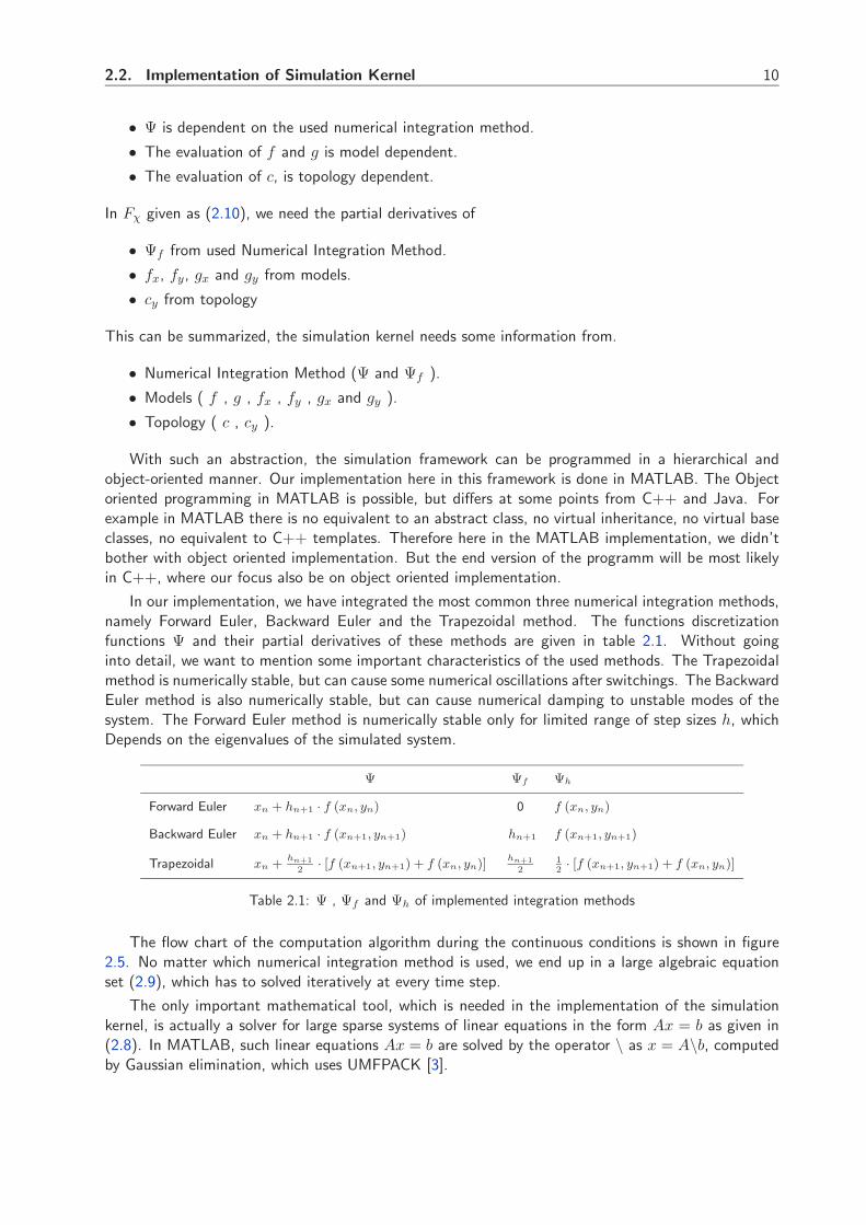
In our implementation, we have integrated the most common three numerical integration methods,namely Forward Euler, Backward Euler and the Trapezoidal method. The functions discretizationfunctions Ψ and their partial derivatives of these methods are given in table 2.1. Without goinginto detail, we want to mention some important characteristics of the used methods. The Trapezoidalmethod is numerically stable, but can cause some numerical oscillations after switchings. The BackwardEuler method is also numerically stable, but can cause numerical damping to unstable modes of thesystem. The Forward Euler method is numerically stable only for limited range of step sizes h, whichDepends on the eigenvalues of the simulated system.
Ψ Ψf Ψh
Forward Euler xn + hn+1 · f (xn, yn) 0 f (xn, yn)
Backward Euler xn + hn+1 · f (xn+1, yn+1) hn+1 f (xn+1, yn+1)
Trapezoidal xn +hn+1
2· [f (xn+1, yn+1) + f (xn, yn)]
hn+12
12· [f (xn+1, yn+1) + f (xn, yn)]
Table 2.1: Ψ , Ψf and Ψh of implemented integration methods
The flow chart of the computation algorithm during the continuous conditions is shown in figure2.5. No matter which numerical integration method is used, we end up in a large algebraic equationset (2.9), which has to solved iteratively at every time step.
The only important mathematical tool, which is needed in the implementation of the simulationkernel, is actually a solver for large sparse systems of linear equations in the form Ax = b as given in(2.8). In MATLAB, such linear equations Ax = b are solved by the operator \ as x = A\b, computedby Gaussian elimination, which uses UMFPACK [3].

2.2. Implementation of Simulation Kernel 11
xn, yn
yes
yes
yes
no
no
no
i = 0 , χi = [xn, yn]
converged = false
converged ?
i < nmaxiter
Calculate F (χi) with (2.9)
|F (χi)| < ε converged = true
calculate Fχ(χi) with (2.10)
compute χi+1 according to (2.8)
i = i + 1
[xn+1, yn+1] = χi
xn+1, yn+1
Figure 2.5: Flow chart during continuous conditions
2.2.3 Event Handling and Consistent Reinitialization
So far, our focus was on the continuous part of the simulation i.e. between events. But as shown infigure 2.1, in such hybrid systems transitions to other modes take place, depending on the transitioncondition. After such a transition, the system is in a new continuous section, where trajectory iscomputed as described in the previous section. In this section, we will describe in detail, how suchtransitions are detected and handled.
As stated before, one of the most important issues in hybrid system simulations is the eventhandling. Event handling is generally done in two stages:
• Event recognition: At this stage, the task is only to detect, whether an event has occurred ornot. The event recognition is warranted by watching the event variables yd and ye of each modelduring simulation process. A sign change of yd and/or zero crossing of ye should be recognizedas an event.
• Event location: If an event has been detected, the simulation kernel must calculate the exactevent time te, where the correspondin event variable becomes zero i.e. yd(te) = 0 or ye(te) = 0.
Figure 2.6 shows the typical trajectory of an event variable. To be able to recognize an event, thesimulation engine must keep track of the event variables. After advancing the solution from tn to tn+1,it should check whether the event variables crossed zero or not. If an event is recognized, the exacttime of the event te must be calculated to make the transition to the new system mode at the correcttime instance. After an event has been recognized some intermediate steps must be taken.
First step is to calculate the exact event time te. Lets assume we are at t = tn and advance thesolution by integrating with step size hn+1 to t = tn+1. And we recognize that the event variable ye
changed sign. At tn it is −, at tn+1 it becomes +. To compute te, we make a small modification in
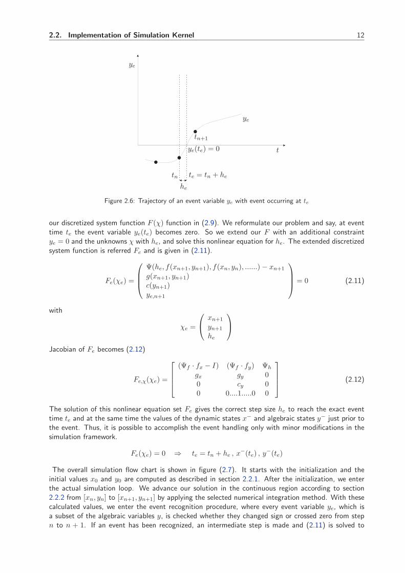
2.2. Implementation of Simulation Kernel 12
ye
ye
te = tn + he
tn+1
tn
t
he
ye(te) = 0
Figure 2.6: Trajectory of an event variable ye with event occurring at te
our discretized system function F (χ) function in (2.9). We reformulate our problem and say, at eventtime te the event variable ye(te) becomes zero. So we extend our F with an additional constraintye = 0 and the unknowns χ with he, and solve this nonlinear equation for he. The extended discretizedsystem function is referred Fe and is given in (2.11).
Fe(χe) =
⎛⎜⎜⎝
Ψ(he, f(xn+1, yn+1), f(xn, yn), ......) − xn+1
g(xn+1, yn+1)c(yn+1)ye,n+1
⎞⎟⎟⎠ = 0 (2.11)
with
χe =
⎛⎝ xn+1
yn+1
he
⎞⎠
Jacobian of Fe becomes (2.12)
Fe,χ(χe) =
⎡⎢⎢⎣
(Ψf · fx − I) (Ψf · fy) Ψh
gx gy 00 cy 00 0....1.....0 0
⎤⎥⎥⎦ (2.12)
The solution of this nonlinear equation set Fe gives the correct step size he to reach the exact eventtime te and at the same time the values of the dynamic states x− and algebraic states y− just prior tothe event. Thus, it is possible to accomplish the event handling only with minor modifications in thesimulation framework.
Fe(χe) = 0 ⇒ te = tn + he , x−(te) , y−(te)
The overall simulation flow chart is shown in figure (2.7). It starts with the initialization and theinitial values x0 and y0 are computed as described in section 2.2.1. After the initialization, we enterthe actual simulation loop. We advance our solution in the continuous region according to section2.2.2 from [xn, yn] to [xn+1, yn+1] by applying the selected numerical integration method. With thesecalculated values, we enter the event recognition procedure, where every event variable ye, which isa subset of the algebraic variables y, is checked whether they changed sign or crossed zero from stepn to n + 1. If an event has been recognized, an intermediate step is made and (2.11) is solved to

2.3. Automatic Code Generator 13
yes
yes
no
no
Initialization
x0, y0, t = 0
t < tend End
Calculate Continuous Conditions
Event detected
Compute he,te,x−(te),y−(te)
according to (2.11)
Compute z+ according to (2.6)
Compute y+ according to (2.5)
Figure 2.7: Flow chart of the overall simulation
determine the exact event time te. The solution of (2.11) gives also the pre-event values x−(te) andy−(te) and thus the current continuous section can be closed by storing these values te, x−(te) andy−(te). The switch to the new system mode takes place in three steps.
• As mentioned before, the continuous dynamic states are continuous at events so that post-eventvalues of the dynamic states can directly given as x+ = x−.
• Then, event values of the discrete states z+ are computed by (2.6) at te with the pre-eventvalues x−, y− and z−.
• Then, with these x+ and z+ state values, we solve (2.5) for determining the post-event algebraicstate values y+.
Thus, all post-event values x+, y+ and z+ are computed, which serve as an initial for the newcontinuous section. The simulation loop lasts till the simulation time t reaches tend.
2.3 Automatic Code Generator
Sofar we described the structure of the simulation kernel of the implemented simulation framework.As discussed in the previous sections, the simulation kernel needs the models be described in theDSAR structure, and for the numerical simulation each model has to provide the kernel with the modelfunctions f , g, h , with their partial derivatives fx, fy, gx, gy and the event variables yd, ye for eventhandling. The described exchange of information is illustrated in figure 2.8. This means the models,which are implemented in MATLAB M-Files, have to compute and return the desired function for givent, x and y. Definitions of the f , g and h are normally given or known. But sometimes the analyticalcalculation of the partial derivatives can be really time consuming.

2.3. Automatic Code Generator 14
Therefore, to ease the model creation for the users, we have implemented a tool called AutomaticCode Generator (ACG) as also proposed in [4]. Actually, the user simply writes the model equationsin the required DSAR structure in a text file called Model Definition File (MDF), by defining the
• continuous dynamic states x
• discrete dynamic states z
• algebraic states y
• event variables yd and ye
• differential equations f
• switched-algebraic equations gi depending on the corresponding yd
• state-reset equations hj depending on the corresponding ye
f ,fx,fy,g,gx,gy,h and yd,ye
f ,fx,fy,g,gx,gy,h and yd,ye
f ,fx,fy,g,gx,gy,h and yd,ye
Simulation Kernelc(y),cy
Ψ,Ψf ,Ψh
t,x,y t,x,y
t,x,y
Model1 Model2
Model3
DSAR DSAR
DSAR
y1,1 y1,2 y2,1 y2,2
y3,1 y3,2
Figure 2.8: Model - Simulation Kernel interface
The ACG takes the MDF of the model and creates the model’s MATLAB M-file by using thesymbolic toolbox of MATLAB for symbolic manipulation and for the analytical calculation of thepartial derivatives.

2.3. Automatic Code Generator 15
Example RC-Circuit
As an example, the model of the RC-circuit given in 2.9 will be treated.The circuit has two states:
−+
Vdc
R
C
Irc
Vc
definitions:
dynamic states Vc
discrete states Vdc
algebraic states Irc
events VC upper VC lower
parameters R C
f equations:
dt(Vc) = Irc/C
dt(Vdc) = 0;
g equations:
g(1)= Vdc − ( Irc · R + Vc)
g(2)= VC upper − (Vc − 5)
g(3)= VC lower − (Vc + 1)
h equations:
if VC upper==0
Vdc = −8
end
if VC lower==0
Vdc = +8
end
Figure 2.9: Example RC-circuit with corresponding MDF
charging and discharging.In charging state, the value of DC is 8 Volt while in discharging state its valuesis -8 Volt. If the capacitor voltage Vc exceeds the upper limit of V upper
c = 5V , the state switches from
General DSAR structure RC-Circuit equations in DSAR
x = f(x, y, z, λ) Vc = IrcC
z = 0 Vdc = 0
0 = Vdc − (Irc · R + Vc)0 = g0(x, y) 0 = V upper
c − (Vc − 5)0 = V lower
c − (Vc + 1)
0 = g(i−)(x, y, z, λ) yd,i < 0
0 = g(i+)(x, y, z, λ) yd,i > 0
z+ = hj(x−, y−, z−, λ) ye,j = 0 j ∈ {1, ...., e} Vdc+ = −8 if V upper
c = 0Vdc
+ = +8 if V lowerc = 0
Table 2.2: RC-Circuit equations in DSAR structure
charging to discharging mode (Vdc = 8 → −8). If the capacitor voltage falls below V lowerc = −1V ,
the state switches from discharging to charging mode (Vdc = −8 → 8). The model equations of thecircuit can be given in the described DSAR structure as given in table 2.2.

2.3. Automatic Code Generator 16
The Model Definition File of this circuit is given in figure 2.9. First we define the variables of themodel, which starts with the keyword ”definitions:”. We have one continuous dynamic state x, thecapacitor voltage Vc, which is defined with the identifier ”dynamic states”. The only discrete state zin this example is the DC Voltage Vdc, defined with the identifier ”discrete states”. The current Irc isthe algebraic state y identified by ”algebraic states”. Now we have to define the two event variablesye with ”events”, which keep track of the capacitor voltage’s upper V upper
c and lower limits V lowerc . If
these limits are hit, we have a switch in our discrete state Vdc. And finally the parameters of the modelλ are defined by the ”parameters” identifier. Thus all the variables and parameters of the model aredefined. Now, we have to define the model definition equations f , g and h. ”f equations:” startsthe input of the differential equations f , ”g equations:” starts the input of the switched algebraicequations g and ”h equations:” starts the input of the state-reset equations h of the model. The”dt()” operator is the derivative operator. In the h equations the line Vdc = −8 means the post-eventvalue of discrete state Vdc becomes −8 (V +
dc = −8).
The described MDF is then fed into the ACG. The ACG creates the Matlab code for the model as anM-file. And this file can be used directly in the simulation framework. Figure 2.10 shows the trajectoryof the Vdc, Vc, and Irc during the simulation with the created model file. With initial conditions Vc0 = 0and Vdc0 = 8
0.0 0.2 0.4 0.6 0.8 1.0-12.0
-8.0
-4.0
0.0
4.0
8.0
VdcVcIrc
t
Figure 2.10: Simulation results of the RC-circuit
With the ACG, the user concentrates only on the generation of model equations and writes themin the required form in a MDF. To bring it into the form, which can be processed by the simulationkernel, is the task of the ACG.
2.4. Summary 17
2.4 Summary
In this chapter, we focused on the implementation of the simulation framework, which has beenalso used in later studies. The implemented simulation framework can be summarized as non-causalmodeling of systems represented by Differential Switched-Algebraic State-Reset Equations (DSAR)[1], including discrete events and event handling. In this framework, every model is fully described bythe model equations given in the DSAR structure, and models are connected together with so calledlinks through their interface variables, which is described a simple mathematical algebraic constraint.The models have to satisfy the model equations and the algebraic connection equations. The overallsystem is then discretized by a numerical integration method. This discretization leads to a large butsparse nonlinear algebraic equation set, which has to be solved iteratively every time step. Numericalintegration methods such as, Forward Euler, Backward Euler and Trapezoidal Integration method hasbeen implemented. A variable time step algorithm is built based on the local truncation error estimate.But the aim is to replace the numerical integration engine by an adapted version of the DASSL routine[5], which uses backward differentiation formula (BDF) methods with variable step-size and variableorder to solve a system of DAEs or ODEs [6]. To ease the creation of models for the user, a tool calledAutomatic Code Generator has been implemented, where the user simply writes the model equationsand the ACG creates the MATLAB code of the model, which can be used by the simulation kernel.Thus one can save a lot of time by model implementation. This tool will also be used in the followingchapters to derive models for power system components.

Chapter 3
Modeling Techniques
The complete power system can be seen as a coupled electromechanical and electromagnetic system.Thus the power system contains a wide range of time constants. There are fast dynamics due to theelectromagnetic phenomena, and slow dynamics due to the electromechanical phenomena. There aresimulation programs, which do full time domain simulations without making any distinction betweenthe different time-scales and consider both, slow and fast dynamics. Such programs are referred to asEMTP like programs in the literature.
Actually, depending on the nature of the study, some simplifying assumptions can be made. Ifour interest is more on the fast phenomena, such as line dynamics or switching behavior of powerelectronic devices, slow dynamics of the electromechanical system can be neglected. But in most ofthe power system studies, the focus is on the slower electromechanical phenomena, so that the fastelectromagnetic transients of the electrical network are neglected. Such studies are made with thetransient stability programs. In these programs, the network quantities are represented as fundamentalfrequency phasor models.
Recent developments, particularly the introduction of more power electronics based equipment e.g.HVDC and FACTS components, show that there is a shortage in the analysis methods with fundamentalfrequency phasor models. For such components a full time domain simulation might be needed. Acomplete representation of a large power system in an electromagnetic transients program is verydifficult and won’t give additional information. To overcome this problem, the concept of time-varyingDynamic phasors is proposed [7] to model power electronics based equipment similar approaches havebeen also reported in [8]. The concept of time-varying dynamic phasors has also been applied analyzeasymmetrical faults [9] and also synchronous and induction machines [10]. It has several advantagesover phasor based methods. Firstly, it has a wider bandwidth in the frequency domain than the quasi-stationary phasor. Secondly, dynamic phasors can be used to compute fast electromagnetic transientswith larger time steps, so that it drastically reduces the simulation time compared with conventionaltime domain EMTP like simulation. Phasor Dynamics Approach provides a middle ground between theapproximations inherent in a phasor based sinusoidal quasi-steady-state representation, and the analyticcomplexity and computational burden associated with representing network voltages and currents intime-domain.
This chapter gives an overview of the different modeling techniques, which are commonly used inproduction-grade programs for modeling of power system components (Figure 3.1). Firstly, we willhandle the power system components in ”true physical” ABC reference frame. After this, we willtake advantage of the periodicity of the balanced three-phase quantities and derive the DQ0 referenceframe models. And finally the inherent periodical switchings of FACTs devices will allow us someuseful approximations by derivation of phasor dynamic models. A detailed introduction to the conceptof time-varying Fourier coefficients will be given, which is used as an analytical tool for deriving dynamicphasor models. Later, we will give an additional application example on the TCSC as described in [7].Finally, reduced order models will be treated, where the fast transients of the electrical network are
18

19
neglected, which is a common approach in transient stability programs. Figure 3.1 shows the differentmodeling techniques.
Modeling
Techniques
ABC Three-Phase
Models
DQ0 Transformed
Models
Dynamic Phasor
Models
Dynamic Phasor
Models
Detailed
Models
Reduced Order
Models
Figure 3.1: Modeling Techniques
The application of the described modeling techniques will be illustrated by the standard Π transmissionline model shown in figure 3.2.
R L
a
b
c
va
ia
Figure 3.2: Circuit diagram of Π transmission line model

3.1. Models in Three-Phase (ABC) Reference Frame 20
3.1 Models in Three-Phase (ABC) Reference Frame
Before we start with modeling in ABC reference frame, we will shortly recall the method of symmetricalcomponents, which is often used in power systems analysis.With the method of symmetrical components, it is possible to express any set of unbalanced three-phase quantities (3.1) as the sum of three symmetrical sets of balanced phasors (3.2), which is depictedin figure 3.3.
iabc(t) =
⎡⎣ Ia cos (ωt + θa)
Ib cos (ωt + θb)Ic cos (ωt + θc)
⎤⎦ (3.1)
iabc(t) = Ip
⎡⎣ cos(ωt + θp)
cos(ωt + θp − 2π3 )
cos(ωt + θp + 2π3 )
⎤⎦ + In
⎡⎣ cos(ωt + θn)
cos(ωt + θn + 2π3 )
cos(ωt + θn − 2π3 )
⎤⎦ + Iz
⎡⎣ cos(ωt + θz)
cos(ωt + θz)cos(ωt + θz)
⎤⎦
↑ ↑ ↑ ↑iabc(t) = iabc,p(t) + iabc,n(t) + iabc,z(t)
(3.2)One set of phasors has the same phase sequence as the system (positive sequence iabc,p), the secondset has the reverse phase rotation (negative sequence iabc,n), and the third set has all the same phase(zero sequence iabc,z).
Positive sequence Negative sequence Zero sequencecomponentscomponentscomponents
ia = ia,p + ia,n + ia,z
ia,p
ia,p
ia,n
ia,n
ia,z
ia,z
ib = ib,p + ib,n + ib,z
ib,p
ib,p
ib,n
ib,n
ib,z
ib,z
ic = ic,p + ic,n + ic,z
ic,p
ic,p
ic,n
ic,n
ic,z
ic,z
Figure 3.3: Unbalanced set of phasors as a sum of balanced phasors
True ”physical” models in three-phase reference frame are the starting point for the modeling tech-niques which will be treated in the following sections. All electrical quantities of the electrical networksuch as voltages, currents etc. and all model equations are given in the three-phase (ABC) referenceframe. Such models are commonly used in EMTP like detailed time-domain simulation programs. In
3.2. Models in DQ0 Reference Frame 21
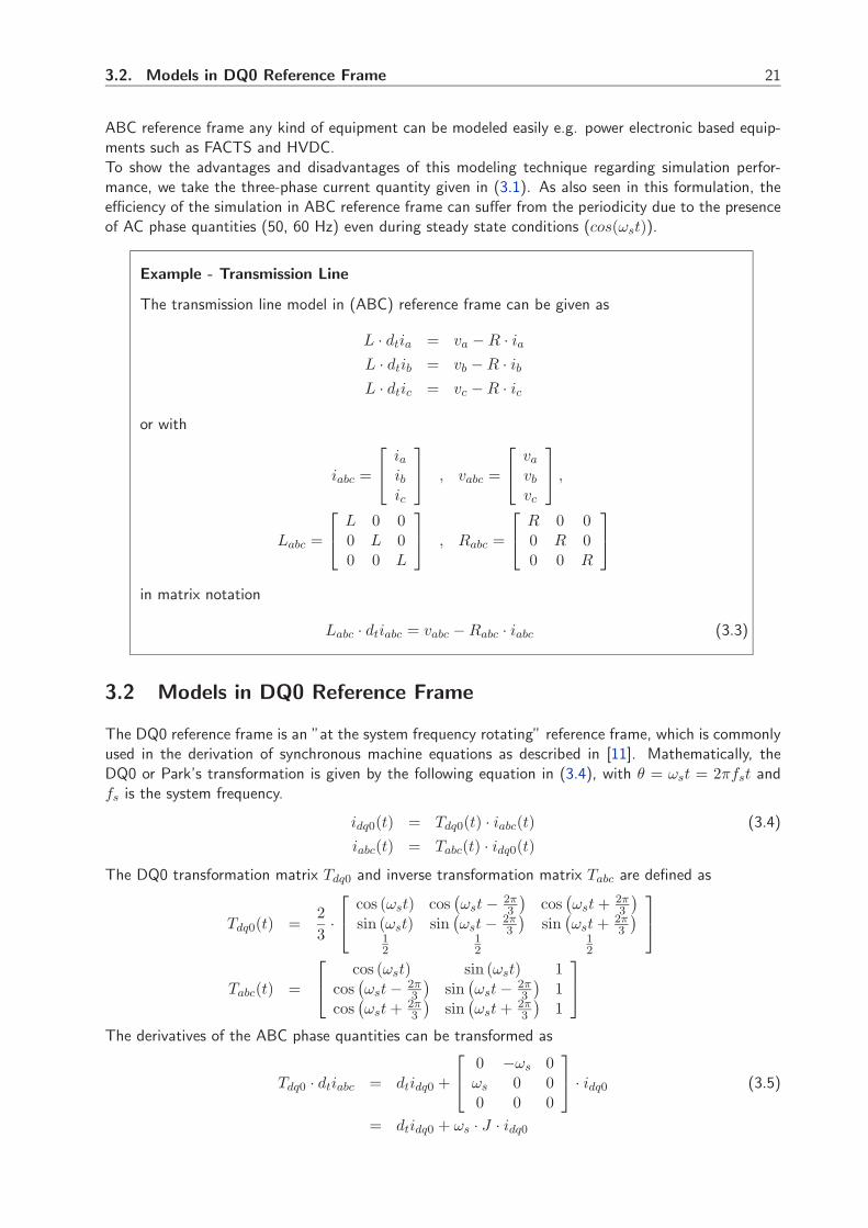
ABC reference frame any kind of equipment can be modeled easily e.g. power electronic based equip-ments such as FACTS and HVDC.To show the advantages and disadvantages of this modeling technique regarding simulation perfor-mance, we take the three-phase current quantity given in (3.1). As also seen in this formulation, theefficiency of the simulation in ABC reference frame can suffer from the periodicity due to the presenceof AC phase quantities (50, 60 Hz) even during steady state conditions (cos(ωst)).
Example - Transmission Line
The transmission line model in (ABC) reference frame can be given as
L · dtia = va − R · iaL · dtib = vb − R · ibL · dtic = vc − R · ic
or with
iabc =
⎡⎣ ia
ibic
⎤⎦ , vabc =
⎡⎣ va
vb
vc
⎤⎦ ,
Labc =
⎡⎣ L 0 0
0 L 00 0 L
⎤⎦ , Rabc =
⎡⎣ R 0 0
0 R 00 0 R
⎤⎦
in matrix notation
Labc · dtiabc = vabc − Rabc · iabc (3.3)
3.2 Models in DQ0 Reference Frame
The DQ0 reference frame is an ”at the system frequency rotating” reference frame, which is commonlyused in the derivation of synchronous machine equations as described in [11]. Mathematically, theDQ0 or Park’s transformation is given by the following equation in (3.4), with θ = ωst = 2πfst andfs is the system frequency.
idq0(t) = Tdq0(t) · iabc(t) (3.4)
iabc(t) = Tabc(t) · idq0(t)
The DQ0 transformation matrix Tdq0 and inverse transformation matrix Tabc are defined as
Tdq0(t) =23·⎡⎣ cos (ωst) cos
(ωst − 2π
3
)cos
(ωst + 2π
3
)sin (ωst) sin
(ωst − 2π
3
)sin
(ωst + 2π
3
)12
12
12
⎤⎦
Tabc(t) =
⎡⎣ cos (ωst) sin (ωst) 1
cos(ωst − 2π
3
)sin
(ωst − 2π
3
)1
cos(ωst + 2π
3
)sin
(ωst + 2π
3
)1
⎤⎦
The derivatives of the ABC phase quantities can be transformed as
Tdq0 · dtiabc = dtidq0 +
⎡⎣ 0 −ωs 0
ωs 0 00 0 0
⎤⎦ · idq0 (3.5)
= dtidq0 + ωs · J · idq0

3.2. Models in DQ0 Reference Frame 22
with
J =
⎡⎣ 0 −1 0
1 0 00 0 0
⎤⎦
One of the advantages in analyzing the synchronous machine equations in DQ0 reference frame is thatunder balanced steady-state operation stator quantities have constant values and for other modes ofbalanced operation this quantities vary slowly with time (2-3 Hz). This can easily be verified by takingthe DQ0 transformation of the general three-phase current iabc, which is given in table 3.1. If the
positive sequence negative sequence zero sequencecomponent component component
iabc(t) = Ip ·⎡⎣ cos (ωst + θp)
cos(ωst + θp − 2π
3
)cos
(ωst + θp + 2π
3
)⎤⎦ In ·
⎡⎣ cos (ωst + θn)
cos(ωst + θn + 2π
3
)cos
(ωst + θn − 2π
3
)⎤⎦ Iz ·
⎡⎣ cos (ωst + θz)
cos (ωst + θz)cos (ωst + θz)
⎤⎦
idq0(t) = Ip ·⎡⎣ cos (θp)
sin (θp)0
⎤⎦ In ·
⎡⎣ cos (2 ωst + θn)− sin (2 ωst + θn)
0
⎤⎦ Iz ·
⎡⎣ 0
0cos (ωst + θz)
⎤⎦
Table 3.1: DQ0 transformations of sequence components of iabc
power system is at steady-state, the steady-state current current contains only the positive sequencecomponent. The DQ0 transformation of this positive sequence component is constant. This leads alsoto faster simulation times under balanced conditions, as the variation of variables in DQ0 referenceframe are much slower than the original variables in three-phase ABC reference frame or even constantat steady-state. Therefore in some programs (e.g. SIMPOW [12]) the DQ0 transformation is applied toall components in the system. All variables and equations of the models in three-phase ABC referenceframe are transformed to DQ0 reference frame. The DQ0 transformation is a single reference frametransformation as the reference frame rotates with system frequency. Therefore the simulations in DQ0reference frame will be efficient around system frequency.
But if there are unbalanced conditions in the system or other harmonics, this efficiency can decreasedrastically. If the three-phase current is unbalanced, it contains all three sequence components. TheDQ0 transformation of the negative sequence component contains cos (2ωst) and sin (2ωst) termsand the DQ0 transformation of the zero sequence component contains cos (ωst) and sin (ωst) terms.During unbalanced conditions, we observe oscillations double system frequency 2 ωs in ’d’ and ’q’coordinates, and oscillations with system frequency ωs in ’0’ coordinate of idq0. From the simulationperformance point of view, this means actually that during unbalanced conditions the step size of thesimulation should be kept small enough to capture the oscillations with the maximum frequency (e.g.2 ωs), which makes the simulation inefficient. This is even worse than the original unbalanced casein ABC reference frame, as the maximum occurring frequency in this formulation is system frequency(e.g. ωs).
3.3. Dynamic Phasor Models 23
Example - Transmission Line
The model equations of the transmission line, in ABC reference frame are given in equa-tion (3.3). With the given transformation, the equations for the transmission line can betransformed as
L · dtid = vd − R · id + ωs · L · iqL · dtiq = vq − R · iq − ωs · L · idL · dti0 = v0 − i0 · R
or with
idq0 =
⎡⎣ id
iqi0
⎤⎦ , vdq0 =
⎡⎣ vd
vq
v0
⎤⎦
Ldq0 =
⎡⎣ L 0 0
0 L 00 0 L
⎤⎦ , Rdq0 =
⎡⎣ R 0 0
0 R 00 0 R
⎤⎦
in matrix notation
Ldq0 · dtidq0 = vdq0 − Rdq0 · idq0 − J · ωs · Ldq0 · idq0 (3.6)
3.3 Dynamic Phasor Models
A real valued periodic signal with period T [ e.g. x(τ) = x(τ − T ) ] can be expressed with a Fourierseries representation of the form given as
x(τ) = Re
{ ∞∑k=0
Xk · ej k ωs τ
}
where ωs = 2π/T and Xk is the kth Fourier coefficient in complex form. It’s important to note, asthe signal x(τ) is periodic the Fourier coefficients Xk are time invariant. In power system steady-stateanalysis, these Fourier coefficients Xk are also referred as phasors.
During transients, we don’t have pure periodic but nearly periodic signals. The idea is now to extendthis approach to nearly periodic signals [13] and to approximate x(τ) in the interval τ ∈ (t−T, t] witha Fourier series representation of the form given in (3.7).
x(τ) = Re
{ ∞∑k=0
Xk(t) · ej k ωs τ
}(3.7)
In this representation, as the signal x(τ) is nearly periodic and since the interval under considerationslides as a function of time, the Fourier coefficients Xk are time varying. This time varying Fouriercoefficients are also referred as dynamic phasors. In this approach we are interested in cases where onlya few coefficients provide a good approximation of the original waveform. Xk(t) can be determined bythe following averaging operations.
Xk(t) =1T
t∫t−T
x(τ) · e−j k ωs τdτ = 〈x〉k (t) (3.8)

3.3. Dynamic Phasor Models 24
As notation, here lowercase letters x(τ) are used for instantaneous variables and uppercase lettersXk(t) for dynamic phasors. Some important properties of dynamic phasors are:
• The relation between the derivatives of x(τ) and the derivatives of Xk(t), which is given in (3.9),where the time argument t has been omitted to avoid the notational cluster. This can easily beverified by differentiating the formula given in (3.7)
〈dtx〉k = dtXk + j · k · ωs · Xk (3.9)
• The product of two time-domain variables equals a discrete time convolution of the two dynamicphasor sets of the variables, which is given in (3.10).
〈x · y〉k =∞∑
l=−∞(Xk−l · Yl) (3.10)
• For real valued signal x, the relationship between Xk and X−k given as:
X−k = conjugate(Xk ) = X∗k (3.11)
Here we have used the complex form representation of the equations. With Xk(t) = Xk,c(t)−j ·Xk,s(t),these can easily be transformed into real form representation given in appendix 5.1, which are also usedin MATLAB implementation. The dynamic phasors approach offers a numbers of advantages overconventional methods.
+ The selection of k gives a wider bandwidth in the frequency domain than traditional slow quasi-stationary assumptions used in Transient Stability Programs.
+ As the variations of dynamic phasors Xk are much slower than the instantaneous quantities x,they can be used to compute the fast electromagnetic transients with larger step series, so thatit makes simulation potentially faster than conventional time domain EMTP like simulation.
+ The time domain simulations of such large systems with periodically switched power electronicbased components have not only a computational burden, but also give little insight into theproblem sensitivities to design controllers or protection schemes. Dynamic phasors approach alsoallows an analytical insight into such problems, as it approximates a periodically switched systemwith a continuous system.
– One disadvantage of the dynamic phasors approach is that the number of variables and equationsin phasor dynamics approach (3.22) is higher than in the original equations (3.21), which makesthe simulation inefficient.
As example we take the three-phase current from the previous sections in ABC and DQ0 referenceframe and apply the phasor dynamics approach to these quantities to verify the advantages and thedisadvantages of the applied method.The question is, which Fourier coefficients should be used for an appropriate approximation in equation(3.7)?In the case of ABC reference frame in (3.2), it’s actually straight forward to approximate with k = {1}.
iabc(τ) ≈ Iabc,1c(t) · cos(ωsτ) + Iabc,1s(t) · sin(ωsτ)
Iabc,1c(t) and Iabc,1s(t) can be calculated by applying equation (3.8) as.

3.3. Dynamic Phasor Models 25
Iabc,1c(t) =
⎡⎢⎢⎣
Ip cos (θp) + In cos (θn) + Iz cos (θz )
−12 Ip cos (θp) +
√3
2 Ip sin (θp) −√
32 In sin (θn) − 1
2 In cos (θn) + Iz cos (θz )
−√
32 Ip sin (θp) − 1
2 Ip cos (θp) − 12 In cos (θn) +
√3
2 In sin (θn) + Iz cos (θz )
⎤⎥⎥⎦
Iabc,1s(t) =
⎡⎢⎢⎣
−Ip sin (θp) − In sin (θn) − Iz sin (θz )
12 Ip sin (θp) +
√3
2 Ip cos (θp) −√
32 In cos (θn) + 1
2 In sin (θn) − Iz sin (θz )
−√
32 Ip cos (θp) + 1
2 Ip sin (θp) + 12 In sin (θn) +
√3
2 In cos (θn) − Iz sin (θz )
⎤⎥⎥⎦
(3.12)
In the case of idq0 in table (3.1), an appropriate selection for the approximation would be k ={0, 1, 2} as unbalanced conditions induce terms with double system frequency in d and q coordinatesand terms with system frequency in 0 coordinates.
idq0(τ) ≈ Idq0,0(t) + Idq0,1c(t) · cos(ωsτ) + Idq0,1s(t) · sin(ωsτ) +Idq0,2c(t) · cos(2 ωsτ) + Idq0,2s(t) · sin(2ωsτ)
The Fourier coefficients Idq0,0(t), Idq0,1c(t), Idq0,1s(t), Idq0,2c(t), Idq0,2s(t) are given as
Idq0,0(t) =
⎡⎣ Ip cos (θp)
Ip sin (θp)0
⎤⎦
Idq0,1c(t) =
⎡⎣ 0
0Iz cos (θz)
⎤⎦
Idq0,1s(t) =
⎡⎣ 0
0−Iz sin (θz)
⎤⎦
Idq0,2c(t) =
⎡⎣ In cos (θn)
−In sin (θn)0
⎤⎦
Idq0,2c(t) =
⎡⎣ −In sin (θn)
−In cos (θn)0
⎤⎦ (3.13)
The Fourier coefficient Idq0,0(t) contains the positive-sequence, Idq0,1c(t) and Idq0,1s(t) the zero-sequence, Idq0,2c(t) and Idq0,2s(t) the negative-sequence components of the three-phase current.If we have balanced conditions, only positive sequence components will exist. Thus Idq0,1c(t), Idq0,1s(t),Idq0,2c(t) and Idq0,2s(t) become all zero.
The Fourier coefficients in (3.12) and (3.13) are all constant even during unbalanced conditions.This was not the case in ABC reference frame [equation 3.2] and DQ0 reference frame [table 3.1].The variations of the Fourier coefficients are much slower than the instantaneous quantities and evenconstant during unbalanced conditions, which allows larger step sizes during simulation process. Oneadvantage of the DQ0 based dynamic phasor model is the achieved the decoupling of the sequencequantities (3.13). In ABC-based dynamic phasor models, this is not the case (3.12).
Another important point is, that with the dynamic phasors approach, the number of variablesactually increase compared to original ABC reference frame or DQ0 reference frame. For example, inABC reference frame we have 3 variables (one per phase), in DQ0 reference frame also 3 variables (one

3.3. Dynamic Phasor Models 26
per axis d, q, 0). But in dynamic phasors approach the number of variables depends on the selection ofk. For example here in ABC reference frame based dynamic phasor models (3.12) with k = {1}, wehave 6 variables and in DQ0 reference frame based dynamic phasor models (3.13) with k = {0, 1, 2},we have 15 variables. This increase leads also to a higher number of equations which have to be solvedduring the simulation process and decreases the simulation performance. But the efficiency gain due toslower variations in the Fourier coefficients is mostly higher than the efficiency loss due to the increasednumber of variables and equations.
Example - Transmission Line
The model equations of the transmission line, in ABC reference frame are given in equation(3.3). Rewriting these equations with the appropriate approximation (k = {1}) and applyingtransformation rules given in appendix 5.1, the new the ABC reference frame based phasordynamics model equations of the transmission line become,
L · dtIa,1c = Va,1c − R · Ia,1c − ωs · L · Ia,1s
L · dtIa,1s = Va,1s − R · Ia,1s + ωs · L · Ia,1c
L · dtIb,1c = Vb,1c − R · Ib,1c − ωs · L · Ib,1s
L · dtIb,1s = Vb,1s − R · Ib,1s + ωs · L · Ib,1c
L · dtIc,1c = Vc,1c − R · Ic,1c − ωs · L · Ic,1s
L · dtIc,1s = Vc,1s − R · Ic,1s + ωs · L · Ic,1c (3.14)
The model equations of the transmission line, in ABC reference frame are given in equation(3.6). The DQ0 reference frame based phasor dynamics model equations of the transmissionline, with the appropriate approximation (k = {0, 1, 2}), are given as
L · dtId,0 = Vd,0 − R · Id,0 + ωs · L · Iq,0
L · dtIq,0 = Vq,0 − R · Iq,0 − ωs · L · Id,0
L · dtI0,0 = V0,0 − R · I0,0
L · dtId,1c = Vd,1c − R · Id,1c + ωs · L · Iq,1c − ωs · L · Id,1s
L · dtIq,1c = Vq,1c − R · Iq,1c − ωs · L · Id,1c − ωs · L · Iq,1s
L · dtI0,1c = V0,1c − R · I0,1c − ωs · L · I0,1s
L · dtId,1s = Vd,1s − R · Id,1s + ωs · L · Iq,1s + ωs · L · Id,1c
L · dtIq,1s = Vq,1s − R · Iq,1s − ωs · L · Id,1s + ωs · L · Iq,1c
L · dtI0,1s = V0,1s − R · I0,1s + ωs · L · I0,1c
L · dtId,2c = Vd,2c − R · Id,2c + ωs · L · Iq,2c − 2 · ωs · L · Id,2s
L · dtIq,2c = Vq,2c − R · Iq,2c − ωs · L · Id,2c − 2 · ωs · L · Iq,2s
L · dtI0,2c = V0,2c − R · I0,2c − 2 · ωs · L · I0,2s
L · dtId,2s = Vq,2s − R · Iq,2s + ωs · L · Iq,2s + 2 · ωs · L · Id,2c
L · dtIq,2s = Vq,2s − R · Iq,2s − ωs · L · Id,2s + 2 · ωs · L · Iq,2c
L · dtI0,2s = V0,2s − R · I0,2s + 2 · ωs · L · I0,2c (3.15)
3.4. Application Example - TCSC 27
3.4 Application Example - TCSC
This application example is based on the work described in [7]. The idea here is to derive a fundamentalphasor dynamic model by using the described approach.
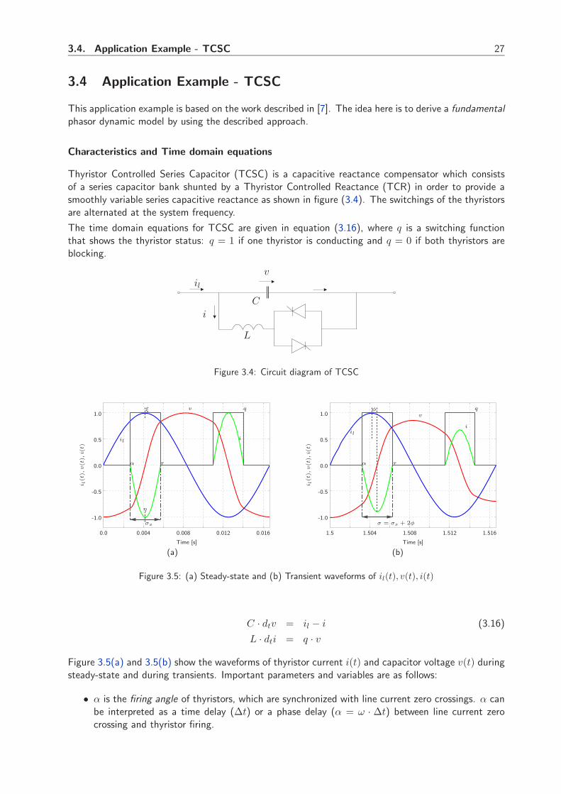
Characteristics and Time domain equations
Thyristor Controlled Series Capacitor (TCSC) is a capacitive reactance compensator which consistsof a series capacitor bank shunted by a Thyristor Controlled Reactance (TCR) in order to provide asmoothly variable series capacitive reactance as shown in figure (3.4). The switchings of the thyristorsare alternated at the system frequency.
The time domain equations for TCSC are given in equation (3.16), where q is a switching functionthat shows the thyristor status: q = 1 if one thyristor is conducting and q = 0 if both thyristors areblocking.
il
i
v
C
L
Figure 3.4: Circuit diagram of TCSC
Time [s]
i l(t
),v(t
),i(
t)
il
v
i
qξ
σs
α τ
η
0.0 0.004 0.008 0.012 0.016
-1.0
-0.5
0.0
0.5
1.0
(a)
Time [s]
i l(t
),v(t
),i(
t)
il
v
i
qφ
σ = σs + 2φ
α τ
1.5 1.504 1.508 1.512 1.516
-1.0
-0.5
0.0
0.5
1.0
(b)
Figure 3.5: (a) Steady-state and (b) Transient waveforms of il(t), v(t), i(t)
C · dtv = il − i (3.16)
L · dti = q · v
Figure 3.5(a) and 3.5(b) show the waveforms of thyristor current i(t) and capacitor voltage v(t) duringsteady-state and during transients. Important parameters and variables are as follows:
• α is the firing angle of thyristors, which are synchronized with line current zero crossings. α canbe interpreted as a time delay (Δt) or a phase delay (α = ω · Δt) between line current zerocrossing and thyristor firing.
3.4. Application Example - TCSC 28
• τ is the angle where the thyristor current recrosses zero and the thyristor switches off.
• ξ is the phase angle corresponding to the peak value of line current ilwith ξ = arg( I∗l ).
• ψ is the phase angle corresponding to the peak value of capacitor voltage vwith ψ = arg(V ∗
1 ).
• φ is phase angle difference given between peak value of line current and the negative peak valueof thyristor current. φ = arg(−Il · I∗1 ). At steady-state φ = 0.
• σs is reference conduction angle (σs/2 = ξ − α ).
• σ is the so called conduction angle given as σ = τ − α = σs + 2φ. In this range the thyristorconducts.
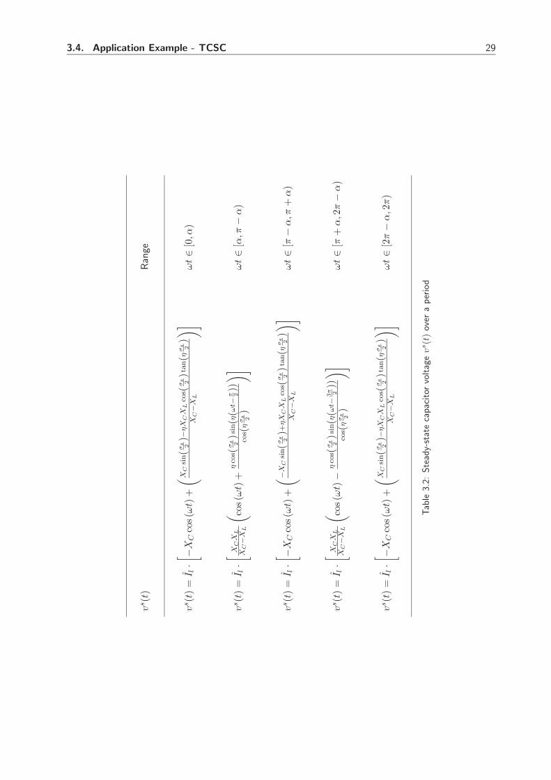
The switching function q in equation (3.16) can be given as, q(θ) = 1 during a period if θ ∈ [α, τ ] andθ ∈ [α + π, τ + π] with θ = ωt. Thus, q is a function of conduction angle q(σ).Before we apply the phasor dynamics approach to these equation, a proper selection of Fourier coef-ficients k in equation 3.7 has to be made for an appropriate approximation of these quantities. Onepossibility is to investigate these quantities (v and i) at steady-state. Assuming, the line current issinusoidal il(t) = Il · sin(ωt), the steady-state analytical expression for v(t) = v(t, α) = v(t, σs) overa period can be written in dependence conduction angle reference σs. These steady-state expressionsfor capacitor voltage v are given in Table 3.2.
XC = 1ωC , XL = ωL, ω0 = 1√
LC, η = ω0
ω
To be able to select the appropriate set of Fourier coefficients for the approximation, we look at theharmonic contents of these quantities during steady-state. For example for steady-state capacitorvoltage vs(t), the kth Fourier coefficient V s
k (σs) can easily be calculated by using the formula in (3.8)and table 3.2 as
V sk (σs) =
1T
T∫0
v(τ, σs) · e−j k ωs τdτ (3.17)
Harmonic Distortion of kth harmonic (ρk) is defined as.
ρk =V s
k
V s1
As given in (3.17), Vk and V1 are dependent on the reference conduction angle σs. Figure 3.6 showthe evolution of the real part of ρk in dependence of σs for different values of k. Imaginary part of ρk
is zero, so that from now on we drop the notation Re{ρk} and write directly ρk instead.
For conduction angle values 0◦ − 40◦ the participation of higher harmonics in steady-state capacitorvoltage v quite low. This means, v is well approximated by the fundamental phasor component V1.
v(τ) ≈ Re{
V1(t) · ej ωs τ}
For conduction angle values 40◦−180◦ the participation of higher harmonics become significant. In thiscase, the effects of these harmonics should be taken into account. As figure 3.6 shows, an appropriateselection of dynamic phasors for a good approximation of v(t) would be with k = {1, 3, 5} in equation(3.7). This would give
v(τ) ≈ Re{
V1 (t) · ej ωs τ + V3(t) · ej 3 ωs τ + V5(t) · ej 5 ωs τ}
Now we will derive two dynamic phasor models of TCSC based on these assumptions for v(τ), todemonstrate the application of the dynamic phasors approach.
3.4. Application Example - TCSC 29
vs(t
)Ran
ge
vs(t
)=
I l·[ −X
Cco
s(ωt)
+( X
Csi
n(σ
s 2)−
ηX
CX
Lco
s (σ
s 2)t
an(η
σs 2)
XC−X
L
)]ωt∈
[0,α
)
vs(t
)=
I l·[ X
CX
LX
C−X
L
( cos(
ωt)
+η
cos (
σs 2)s
in(η
(ωt−
π 2))
cos (
ησ
s 2)
)]ωt∈
[α,π
−α)
vs(t
)=
I l·[ −X
Cco
s(ωt)
+( −X
Csi
n(σ
s 2)+
ηX
CX
Lco
s (σ
s 2)t
an(η
σs 2)
XC−X
L
)]ωt∈
[π−
α,π
+α)
vs(t
)=
I l·[ X
CX
LX
C−X
L
( cos(
ωt)−
ηco
s (σ
s 2)s
in(η
(ωt−
3π 2))
cos (
ησ
s 2)
)]ωt∈
[π+
α,2
π−
α)
vs(t
)=
I l·[ −X
Cco
s(ωt)
+( X
Csi
n(σ
s 2)−
ηX
CX
Lco
s (σ
s 2)t
an(η
σs 2)
XC−X
L
)]ωt∈
[2π−
α,2
π)
Tab
le3.
2:Ste
ady-
stat
eca
pac
itor
voltag
ev
s(t
)ov
era
per
iod

3.4. Application Example - TCSC 30
conduction angle reference σs [◦]
Re{ρ
k}
k = 3
k = 5
k = 7
k = 9
0◦ 20◦ 40◦ 60◦ 80◦ 100◦ 120◦ 140◦ 160◦ 180◦-0.50
-0.40
-0.30
-0.20
-0.10
0.00
0.10
0.20
Figure 3.6: Harmonic Distortion
Standard Fundamental Dynamic Phasor Model
As mentioned also in section 3.3, before we start with the derivation of the phasor dynamic model, wehave to make some valid approximations and assumptions for i, il and v.
• The line current il, capacitor voltage v and thyristor current i are well approximated by thedynamic phasors with k = 1, namely IL,1, V1 and I1.
With these assumptions the equation (3.16) becomes
C · dtV1 = Il − I1 − j · ωs · C · V1
L · dtI1 = 〈q · v〉1 − j · ωs · L · I1 (3.18)
With properties (3.10) and 3.11, the term 〈q · v〉1 is expressed as:
〈q · v〉1 = Q0 · V1 + Q2 · V−1 = Q0 · V1 + Q2 · V ∗1
With equation (3.8), the coefficients Q0 and Q2 of the switching function q shown in figure 3.5(b) canbe calculated as
Q0 = 〈q〉0 =σ
π
Q2 = 〈q〉2 =sin (σ)
π· e−j 2 (ξ+φ)
which leads to the final expression for
〈q · v〉1 =1π
(V1 σ + V ∗
1 sin (σ) e−2 j (ξ+φ))
At steady-state, with d/dt = 0, φ = 0 and ξ = ψ − π/2, the equation (3.16) leads to standardequivalent inductance Leq of the TCR which is also used in the literature.
Leq =V1
j ωs I1= L · π
σ − sin (σ)
As stated before, this model gives satisfactory results only if the conduction angle is small. For highervalues of σ, the model can not reflect the participation of higher harmonics (e.g k = 3, 5) even atsteady-state (Figure 3.6). Because of that, we hope to improve our model by including 3rd and 5th
Fourier coefficients in the approximation v(τ). But we will still consider the fundamental phasor in thederivation.

3.4. Application Example - TCSC 31
Improved Fundamental Dynamic Phasor Model
The only change in our assumptions is:
• The capacitor voltage v is now well approximated by the dynamic phasors with k = {1, 3, 5},namely V1, V3 and V5.
As we are still interested in the fundamental phasor model, the equation 3.18 remains the same, butthe calculation of the term 〈q · v〉1 must be modified, as our assumption on v has changed.
〈q · v〉1 = Q0 · V1 + Q2 · V−1 + Q−2 · V3 + Q4 · V−3 + Q−4 · V5 + Q6 · V−5 (3.19)
= Q0 · V1 + Q2 · V ∗1 + Q∗
2 · V3 + Q4 · V ∗3 + Q∗
4 · V5 + Q6 · V ∗5
The additional Fourier coefficients Q4 and Q6 of q are give as
Q4 = 〈q〉4 =12
sin (2σ)π
· e−j 4 (ξ+φ)
Q6 = 〈q〉6 =13
sin (3σ)π
· e−j 6 (ξ+φ)
As we derive a fundamental dynamic phasor model (k = 1), we can make the assumption that theFourier coefficients V3 and V5 can be approximated with the corresponding phase corrections as
Vk = |V1| · ρk(σ) · e−j k ψ (3.20)
for k = {3, 5} by using the steady-state harmonic distortion factor ρk. With these steady-statecorrections of the 3rd and 5th harmonics the term (3.19) is completely defined. The detailed expressionfor ρk(σ) can be found in appendix 5.2.
This model gives a corrected version of V1. The envelope of the detailed time domain signal v(t)can be traced by a corrected version of V1, here called V1, given as
V1 = |V1| · [1 + ρ3(σ) + ρ5(σ)]
Results
The derived dynamic phasor models have been implemented in MATLAB. The detailed time domainsimulation are done with PLECS. PLECS [14] is a toolbox for high-speed simulations of electrical andpower electronic circuits under MATLAB/Simulink. To test the dynamic behavior of the TCSC, weused the same example as in [7] shown in figure 3.7 with the same data: C = 176.84μF , L = 6.8mH,il = Il · sin(ωt), Il = 1kA, ω = 2πf , f = 60Hz.
il
C = 176.84μF
L = 6.8mH
Figure 3.7: Test case for TCSC
The dynamic behavior of the TCSC for changes in the line current magnitude Il and both firing angleα and reference conduction angle σs respectively (σs = π − 2α) is tested with the following eventsequence given in Table 3.3.
Capacitor voltage response to these changes are illustrated in Figure 3.8, where

3.4. Application Example - TCSC 32
t[s] Il[kA] α[◦] σs[◦] = 180◦ − 2α[◦]0.5 1.00 → 1.25 57 661.0 1.25 → 1.00 57 661.5 1.00 57 → 70 66 → 402.0 1.00 70 → 57 40 → 66
Table 3.3: Sequence of events
• v is the capacitor voltage response simulated with PLECS.
• V1 is the fundamental phasor response with standard phasor dynamic model.
• V1 is the corrected fundamental phasor response, which traces the envelope of capacitor voltageresponse v(t).
time [s]
v[k
V]
I II III IV V
v
V1
V 1
−40
−20
0
20
40
0.0 0.5 1.0 1.5 2.0 2.5 3.0
(a)time [s]
v[k
V]
15
20
25
30
35
40
2.0 2.2 2.4 2.6 2.8
(b)
Figure 3.8: Capacitor voltage of the TCSC (a) whole simulation interval (b) zoomed section
These results show, that the standard phasor dynamic model gives only good results in section IV,where we have lower conduction angles, here for σs = 40◦, as the participation of higher harmonics inthis range is quite low (Figure 3.6). In the remaining sections, the standard model doesn’t give correctresults, as for higher conduction angle values the participation of higher harmonics increase, here forσs = 66◦.The improved phasor dynamic model with steady state correction of V1 gives better results in allsections (I-V), as it considers the participation of higher harmonics as well.
Simulation results, where the improved model is used in real power system network, will be given later.
3.5. Modeled Components 33
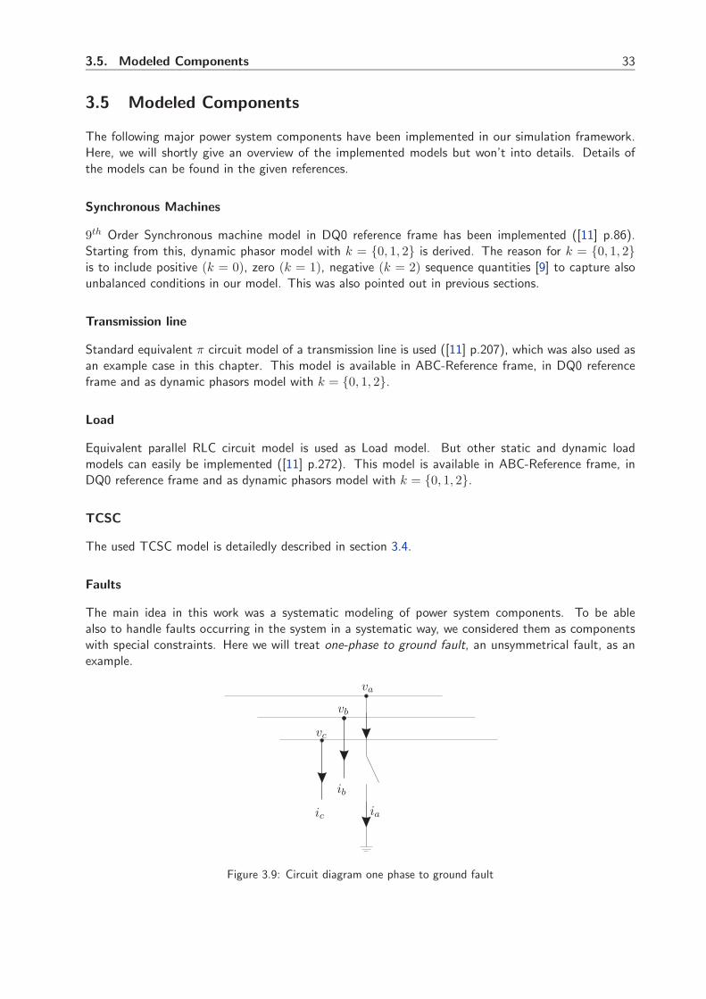
3.5 Modeled Components
The following major power system components have been implemented in our simulation framework.Here, we will shortly give an overview of the implemented models but won’t into details. Details ofthe models can be found in the given references.
Synchronous Machines
9th Order Synchronous machine model in DQ0 reference frame has been implemented ([11] p.86).Starting from this, dynamic phasor model with k = {0, 1, 2} is derived. The reason for k = {0, 1, 2}is to include positive (k = 0), zero (k = 1), negative (k = 2) sequence quantities [9] to capture alsounbalanced conditions in our model. This was also pointed out in previous sections.
Transmission line
Standard equivalent π circuit model of a transmission line is used ([11] p.207), which was also used asan example case in this chapter. This model is available in ABC-Reference frame, in DQ0 referenceframe and as dynamic phasors model with k = {0, 1, 2}.
Load
Equivalent parallel RLC circuit model is used as Load model. But other static and dynamic loadmodels can easily be implemented ([11] p.272). This model is available in ABC-Reference frame, inDQ0 reference frame and as dynamic phasors model with k = {0, 1, 2}.
TCSC
The used TCSC model is detailedly described in section 3.4.
Faults
The main idea in this work was a systematic modeling of power system components. To be ablealso to handle faults occurring in the system in a systematic way, we considered them as componentswith special constraints. Here we will treat one-phase to ground fault, an unsymmetrical fault, as anexample.
va
vb
vc
ia
ib
ic
Figure 3.9: Circuit diagram one phase to ground fault
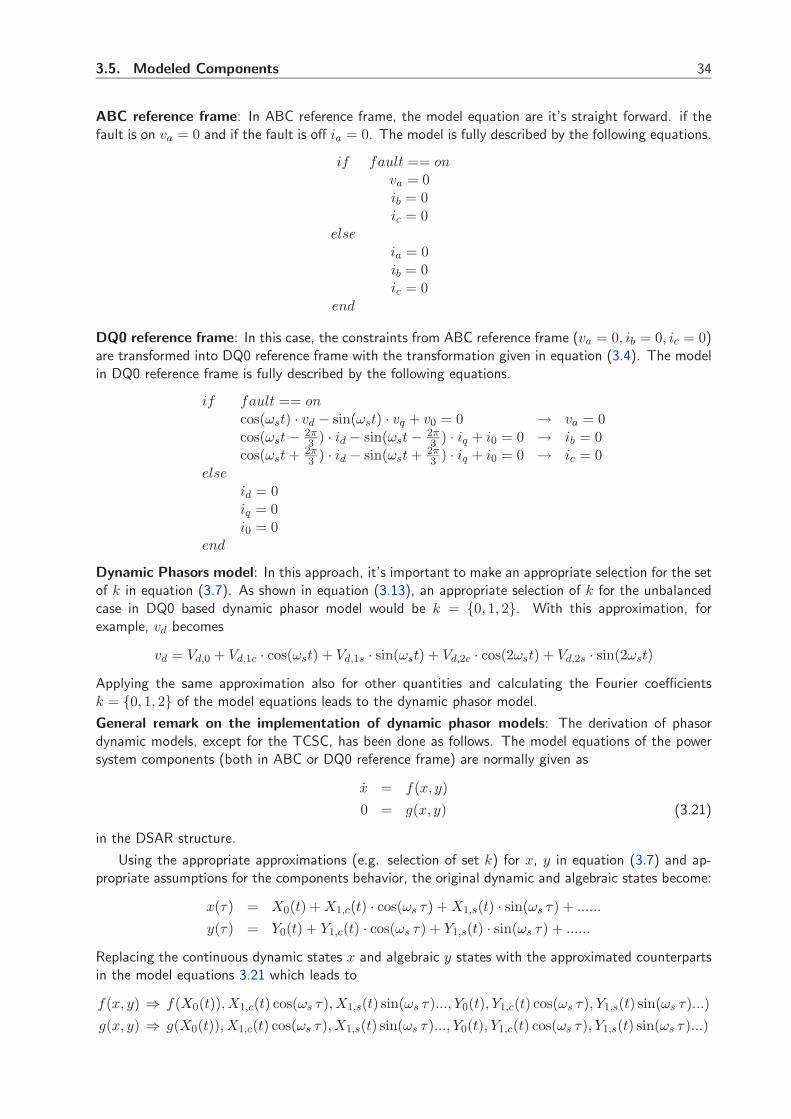
3.5. Modeled Components 34
ABC reference frame: In ABC reference frame, the model equation are it’s straight forward. if thefault is on va = 0 and if the fault is off ia = 0. The model is fully described by the following equations.
if fault == onva = 0ib = 0ic = 0
elseia = 0ib = 0ic = 0
end
DQ0 reference frame: In this case, the constraints from ABC reference frame (va = 0, ib = 0, ic = 0)are transformed into DQ0 reference frame with the transformation given in equation (3.4). The modelin DQ0 reference frame is fully described by the following equations.
if fault == oncos(ωst) · vd − sin(ωst) · vq + v0 = 0 → va = 0cos(ωst − 2π
3 ) · id − sin(ωst − 2π3 ) · iq + i0 = 0 → ib = 0
cos(ωst + 2π3 ) · id − sin(ωst + 2π
3 ) · iq + i0 = 0 → ic = 0else
id = 0iq = 0i0 = 0
end
Dynamic Phasors model: In this approach, it’s important to make an appropriate selection for the setof k in equation (3.7). As shown in equation (3.13), an appropriate selection of k for the unbalancedcase in DQ0 based dynamic phasor model would be k = {0, 1, 2}. With this approximation, forexample, vd becomes
vd = Vd,0 + Vd,1c · cos(ωst) + Vd,1s · sin(ωst) + Vd,2c · cos(2ωst) + Vd,2s · sin(2ωst)
Applying the same approximation also for other quantities and calculating the Fourier coefficientsk = {0, 1, 2} of the model equations leads to the dynamic phasor model.
General remark on the implementation of dynamic phasor models: The derivation of phasordynamic models, except for the TCSC, has been done as follows. The model equations of the powersystem components (both in ABC or DQ0 reference frame) are normally given as
x = f(x, y)0 = g(x, y) (3.21)
in the DSAR structure.
Using the appropriate approximations (e.g. selection of set k) for x, y in equation (3.7) and ap-propriate assumptions for the components behavior, the original dynamic and algebraic states become:
x(τ) = X0(t) + X1,c(t) · cos(ωs τ) + X1,s(t) · sin(ωs τ) + ......
y(τ) = Y0(t) + Y1,c(t) · cos(ωs τ) + Y1,s(t) · sin(ωs τ) + ......
Replacing the continuous dynamic states x and algebraic y states with the approximated counterpartsin the model equations 3.21 which leads to
f(x, y) ⇒ f(X0(t)), X1,c(t) cos(ωs τ), X1,s(t) sin(ωs τ)..., Y0(t), Y1,c(t) cos(ωs τ), Y1,s(t) sin(ωs τ)...)g(x, y) ⇒ g(X0(t)), X1,c(t) cos(ωs τ), X1,s(t) sin(ωs τ)..., Y0(t), Y1,c(t) cos(ωs τ), Y1,s(t) sin(ωs τ)...)

3.6. Reduced Order Models 35
By using the properties (3.8-3.11) in real form given in appendix 5.1, we can transform the set of fand g equations of the model into a new set of equations and get the definition of the dynamic phasormodel in a new set of functions F and G as,
x = f(x, y)0 = g(x, y)
⇒Xk,c = Fk,c(Xk,c, Xk,s, Yk,c, Yk,s) − k · ωs · Xk,s
Xk,s = Fk,s(Xk,c, Xk,s, Yk,c, Yk,s) + k · ωs · Xk,c
0 = Gk,c(Xk,c, Xk,s, Yk,c, Yk,s)0 = Gk,s(Xk,c, Xk,s, Yk,c, Yk,s)
(3.22)
where dynamic phasors Xk become the new continuous dynamic states and Yk the new algebraic states.To automate the creation of the dynamic phasor models from their ABC or DQ0 models, we built in aninterface called Dynamic Phasor Model Generator. The inputs to this interface are the model equations(3.21) in ABC or DQ0 form as MDF (Model Definition File) and the set of k for the approximation.Using the Symbolic Toolbox of MATLAB, the interface creates the MDF of the dynamic phasor model,given in Xk, Yk, Fk and Gk as an output.
3.6 Reduced Order Models
In the previous sections, our focus was on modeling techniques, where we took advantage of someimportant characteristics of the power system. For example the balanced conditions and periodicityof the AC phase quantities led us to the DQ0 transformation, and the (switched) periodicity of theFACTS devices to the dynamic phasors approach. So far we didn’t make any simplification due to thewide range of time constant comprised in power systems. As mentioned before, there are fast dynamicsdue to the electromagnetic phenomena, and slow dynamics due to the electromechanical phenomenain the system. Till now our models captured both phenomena. As next step, we will derive models,where our interest is only on the slow electromechanical phenomena. So, we make an eigenanalysisand a time-scale decomposition to reduce the order of the derived models. We look at the eigenvaluesand their participation factors. Dynamics of continuous states with very low participation in the slowmodes will be neglected, which means for those continuous dynamic states the derivatives (dt x) inmodel equations are set to zero and so they become algebraic states (y). This leads to neglecting thefast transients due to the electromagnetic phenomena in the power system.
DQ0 reference frame models
Let’s take as an example the detailed DQ0 reference frame model of the transmission line given in(3.6). Neglecting the dynamics of the line current in DQ0 reference frame (dtidqo = 0) gives
0 = vd − R · id + ωs · L · iq0 = vq − R · iq − ωs · L · id0 = v0 − i0 · R
with V = vd + jvq, I = id + jiq and zero component ignored, we can reformulate this equation asV = (R + jωsL) · I = ZLine · I. The impedance ZLine is referred as positive sequence impedance ofthe transmission line and is used in the transient stability programs.
This assumption is only valid for balanced conditions as seen in table (3.1). If we have balancedconditions in the system, the current quantity in DQ0 reference frame will contain only positive sequencecomponent, which is constant and so time independent.
But if we have unbalanced conditions in the system, the current quantity in DQ0 reference framewill contain all sequence components, where the negative sequence component has oscillations with2ωs and zero sequence with ωs. Thus this quantities are time dependent, so that the assumption ofdtidqo = 0 is only valid for positive sequence component, but not valid for negative and zero sequence

3.6. Reduced Order Models 36
component. Thus, neglecting fast transients by setting dtidqo = 0 means actually, ignoring the effectof negative and zero sequence quantities.
Therefore, in transient stability programs only positive sequence network is simulated and onlybalanced conditions can be treated. Simulation of unbalanced conditions during unbalanced faults,e.g. one-phase to ground fault, are treated as follows:At fault point, the effects of negative and zero sequence network in the positive-sequence network aretaken into account by appropriately combining the equivalent negative and zero sequence impedancesdepending on the fault-type as described in [11]. Than, this impedance is added to the normal faultimpedance and a three-phase to ground fault is simulated, which is a balanced operation. Actually anunbalanced fault is transformed into a balanced fault. Figure 3.10 taken from [11] shows the describedprocedure.
Pos. seq. Network
Fault Fault Type Zef
Line-to-ground Z2 + Z0
Line-to-line Z2
Double Line-to-ground Z2·Z0Z2+Z0
Three-phase 0
Vpos
Zef
Ipos
Figure 3.10: Fault representation in transient stability programs
Here we treated the transmission line example. Such a order reduction in synchronous machine equa-tions, leads to neglecting the stator flux transients Ψd, Ψq, Ψ0 i.e. setting their derivatives to zero.
3.6. Reduced Order Models 37
Dynamic phasor models
The dynamic phasor model of the transmission line model based on the DQ0 model is given in(3.15).Neglecting the dynamics of the line current gives
0 = Vd,0 − R · Id,0 + ωs · L · Iq,0
0 = Vq,0 − R · Iq,0 − ωs · L · Id,0
0 = V0,0 − R · I0,0
0 = Vd,1c − R · Id,1c + ωs · L · Iq,1c − ωs · L · Id,1s
0 = Vq,1c − R · Iq,1c − ωs · L · Id,1c − ωs · L · Iq,1s
0 = V0,1c − R · I0,1c − ωs · L · I0,1s
0 = Vd,1s − R · Id,1s + ωs · L · Iq,1s + ωs · L · Id,1c
0 = Vq,1s − R · Iq,1s − ωs · L · Id,1s + ωs · L · Iq,1c
0 = V0,1s − R · I0,1s + ωs · L · I0,1c
0 = Vd,2c − R · Id,2c + ωs · L · Iq,2c − 2 · ωs · L · Id,2s
0 = Vq,2c − R · Iq,2c − ωs · L · Id,2c − 2 · ωs · L · Iq,2s
0 = V0,2c − R · I0,2c − 2 · ωs · L · I0,2s
0 = Vq,2s − R · Iq,2s + ωs · L · Iq,2s + 2 · ωs · L · Id,2c
0 = Vq,2s − R · Iq,2s − ωs · L · Id,2s + 2 · ωs · L · Iq,2c
0 = V0,2s − R · I0,2s + 2 · ωs · L · I0,2c
This assumption is valid for balanced and unbalanced conditions. As seen in (3.13), this expressionfor both is constant, and so time independent, for both, balanced and unbalanced conditions.Besides, this assumption doesn’t ignore the effect of negative and zero sequence quantities as it isthe case in the DQ0 reduced order models. With dynamic phasors representation with k = {0, 1, 2},positive- (k = 0), negative- (k = 2) and zero- (k = 1) sequence quantities of the network are allcaptured. Setting (dtIdq0,kc = 0 and dtIdq0,ks = 0) means only neglecting their dynamics but nottheir existence, where in the previous section setting (dtidq0 = 0) means neglecting the dynamics ofpositive sequence current and at the same time ignoring the negative and zero sequence quantities inthe network. As all sequences are modeled in this representation, also unbalanced conditions can betreated directly and more systematically.
3.7. Summary 38
3.7 Summary
In this chapter, we compared different modeling techniques with each other. We can summarize theadvantage and this advantages of these techniques as follow:
• ABC reference frame models:
+ Any kind of equipment can be modeled with this approach.
+ As it takes the ”true physical” model the simulations are accurate.
− For large power systems, the simulations can be in efficient as all components are modelledin detail.
• DQ0 reference frame models:
+ The models in DQ0 reference frame give also accurate results. Because, these models arederived by a transformation and not an approximation.
+ Simulations with these models are efficient if the system is in a balanced condition. In thiscase, only positive sequence network is simulated. The variations of the DQ0 transformedpositive sequence quantities are much slower than the instantaneous values of the quantitiesin ABC reference frame, so that they can be simulated with larger step sizes.
− But, if the system is in an unbalanced condition, negative and zero sequence componentsoccur in the system, with 2ωs and ωs oscillations. This makes the simulations inefficient asthe step size must be kept small enough to come up with these oscillations.
− DQ0 transformation is a single reference frame transformation. Thus it’s only efficient atfundamental frequency or near to fundamental frequency. If there are other harmonics inthe system (e.g. due to FACTS devices), this efficiency will decrease drastically.
• Dynamic phasor models:
+ The accuracy of the simulation is dependent on the appropriate selection of Fourier coeffi-cients k.
+ Simulations with phasor dynamics are efficient as, we are simulating Fourier coefficientsand their variations are much slower than the instantaneous values. Thus, simulations getfaster.
+ Dynamic phasors approach can be interpreted as an orthogonal signal expansion applied tothe complete model, where k gives considered basis functions.
+ Dynamic phasors approach applied to power electronic devices transform the periodicallyswitched system into continuous system, so that we gain more analytical insight (eigenvalueanalysis).
− The number of the variables and equations can increase depending on the selection of k.This can make simulations inefficient.
In the next chapter, we will use these differently derived models in different test systems and verifyour results qualitatively.

Chapter 4
Results
In this chapter, we will try to verify the theoretical results we concluded in the previous chapter, byimplementing and simulating the differently modeled components in a common simulation framework.As test cases, we use the ”Two Area” system and ”Single Machine Infinite Bus” system, with the datagiven in [11]. First, we will make simulations with detailed models and than with reduced order models.
4.1 Simulations with Detailed Models
4.1.1 SMIB system
INFEEDLINE1
LINE2
LINE3
BUS324 kVBUS2
24 kV
GEN
BUS124 kV
Figure 4.1: Single-line diagram of SMIB system
Single line diagram of the network is shown in figure 4.1. An one-phase to ground fault is appliedas a disturbance at 0.1 s BUS2 and removed at 0.17 s. We have simulated this system in our ownsimulation framework with ABC, DQ0 and Dynamic phasor models with k = {0, 1, 2}. The correctnessof the results has been verified by implementing and simulating the same system in PLECS [14].Achieved results are shown in figure 4.2(a), 4.2(b) and 4.2(c). We see a very good overall agreementbetween all results, especially in the zoomed sections. The simulation times for ABC, DQ0 and Dynamicphasor simulations are given in table 4.1. As we see in the results the simulation time with DQ0 is thefastest. The reason for this is, even though we have unbalanced fault it only last for 0.07 second butduring the rest of the simulation ( 4.93 seconds ) we have balanced conditions and during the balancedconditions the DQ0 models are the most efficient ones for the simulation. The dynamic phasor modelswith k = {0, 1, 2} are also more efficient than the ABC models but less efficient than the DQ0 models.The reason for this less efficiency is actually the increased number of variables with dynamic phasorsapproach.
But if we compare the simulation times during the unbalanced conditions, the phasor dynamicsmodels show a better performance than the DQ0 models. During unbalanced conditions, negative andzero sequence quantities arise and in DQ0 models they appear as oscillations with 2ωs and ωs so that
39

4.1. Simulations with Detailed Models 40
time
Te
ofG
EN
1-
[pu]
0.0 1.0 2.0 3.0 4.0 5.0
-1.0
-0.5
0.0
0.5
1.0
1.5
2.0
ABC
DQ0
PHDYN
PLECS
(a)
time
Te
ofG
EN
-[p
u]
0.10 0.12 0.14 0.16 0.18 0.20 0.22 0.24
-1.0
-0.5
0.0
0.5
1.0
1.5
2.0
ABC
DQ0
PHDYN
PLECS
(b)
time
Te
ofG
EN
1-
[pu]
3.0 3.4 3.8 4.2 4.6 5.00.76
0.80
0.84
0.88
0.92
0.96
1.00
ABC
DQ0
PHDYN
PLECS
(c)
Figure 4.2: Electrical Torque of GEN (a) whole simulation (b) during fault (c) after fault
and simulation time is marginally influenced. But with phasor dynamics approach only the envelopeof these negative and zero sequence quantities are simulated, which have much slower variations andthus, can be calculated more efficiently.
The simulations with ABC models are not efficient but show same performance during balancedand unbalanced conditions.
ABC DQ0 k= (0,1,2)
SMIB 121 sec 20 sec 32 sec
Table 4.1: Simulation times for SMIB
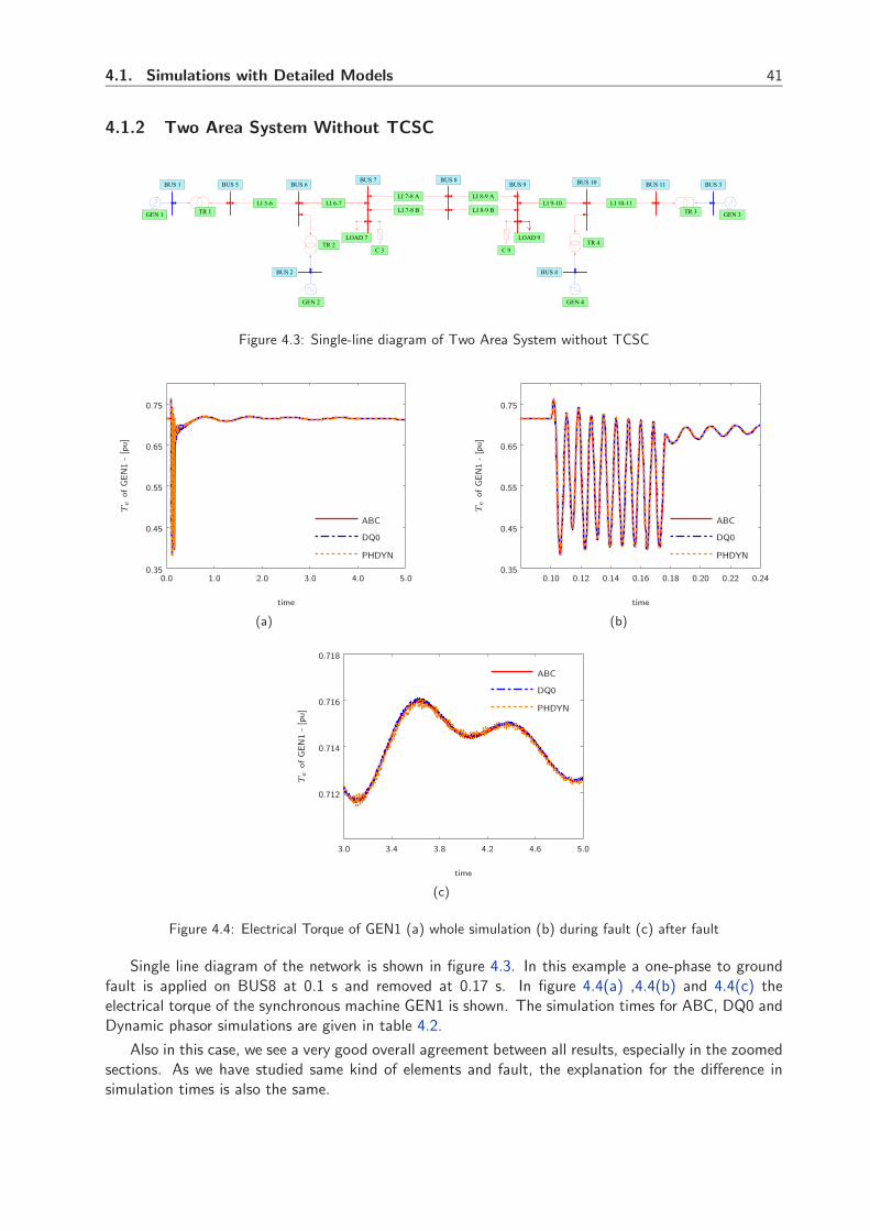
4.1. Simulations with Detailed Models 41
4.1.2 Two Area System Without TCSC
LI 5-6LI 7-8 B LI 8-9 B
LI 9-10 LI 10-11LI 6-7LI 7-8 A LI 8-9 A
TR 1 TR 3
TR 2 TR 4
GEN 1 GEN 3
GEN 2 GEN 4
LOAD 7 LOAD 9
C 3 C 9
BUS 8BUS 5 BUS 11BUS 6 BUS 10BUS 1 BUS 3
BUS 2 BUS 4
BUS 7BUS 9
Figure 4.3: Single-line diagram of Two Area System without TCSC
time
Te
ofG
EN
1-
[pu]
0.0 1.0 2.0 3.0 4.0 5.00.35
0.45
0.55
0.65
0.75
ABC
DQ0
PHDYN
(a)
time
Te
ofG
EN
1-
[pu]
0.10 0.12 0.14 0.16 0.18 0.20 0.22 0.240.35
0.45
0.55
0.65
0.75
ABC
DQ0
PHDYN
(b)
time
Te
ofG
EN
1-
[pu]
3.0 3.4 3.8 4.2 4.6 5.0
0.712
0.714
0.716
0.718
ABC
DQ0
PHDYN
(c)
Figure 4.4: Electrical Torque of GEN1 (a) whole simulation (b) during fault (c) after fault
Single line diagram of the network is shown in figure 4.3. In this example a one-phase to groundfault is applied on BUS8 at 0.1 s and removed at 0.17 s. In figure 4.4(a) ,4.4(b) and 4.4(c) theelectrical torque of the synchronous machine GEN1 is shown. The simulation times for ABC, DQ0 andDynamic phasor simulations are given in table 4.2.
Also in this case, we see a very good overall agreement between all results, especially in the zoomedsections. As we have studied same kind of elements and fault, the explanation for the difference insimulation times is also the same.
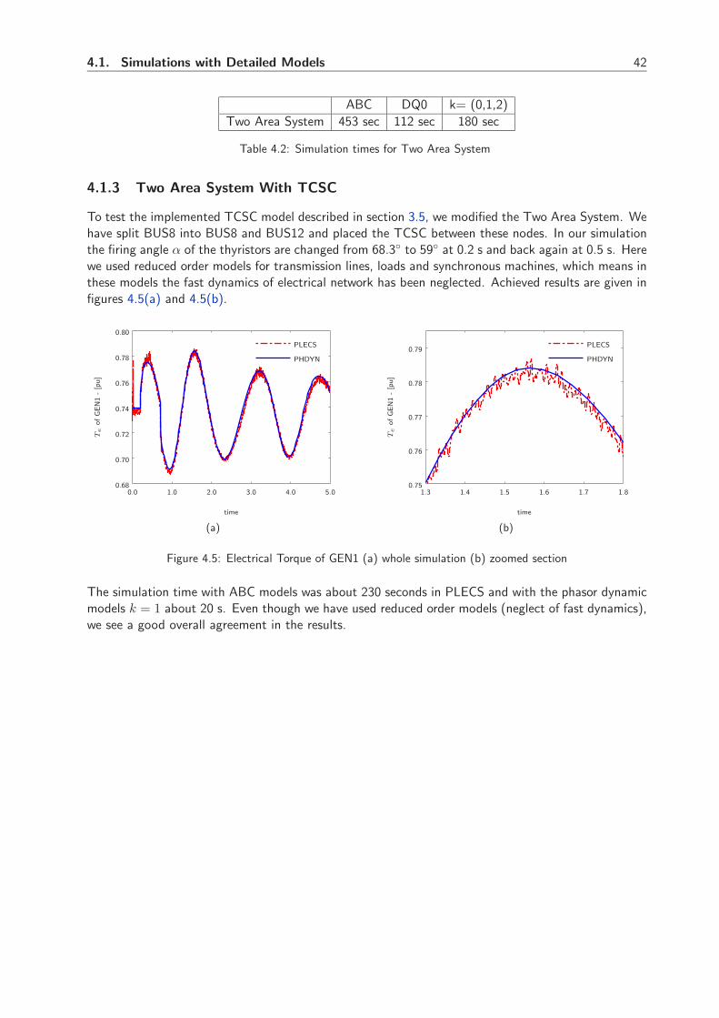
4.1. Simulations with Detailed Models 42
ABC DQ0 k= (0,1,2)
Two Area System 453 sec 112 sec 180 sec
Table 4.2: Simulation times for Two Area System
4.1.3 Two Area System With TCSC
To test the implemented TCSC model described in section 3.5, we modified the Two Area System. Wehave split BUS8 into BUS8 and BUS12 and placed the TCSC between these nodes. In our simulationthe firing angle α of the thyristors are changed from 68.3◦ to 59◦ at 0.2 s and back again at 0.5 s. Herewe used reduced order models for transmission lines, loads and synchronous machines, which means inthese models the fast dynamics of electrical network has been neglected. Achieved results are given infigures 4.5(a) and 4.5(b).
time
Te
ofG
EN
1-
[pu]
0.0 1.0 2.0 3.0 4.0 5.00.68
0.70
0.72
0.74
0.76
0.78
0.80
PLECS
PHDYN
(a)
time
Te
ofG
EN
1-
[pu]
1.3 1.4 1.5 1.6 1.7 1.80.75
0.76
0.77
0.78
0.79PLECS
PHDYN
(b)
Figure 4.5: Electrical Torque of GEN1 (a) whole simulation (b) zoomed section
The simulation time with ABC models was about 230 seconds in PLECS and with the phasor dynamicmodels k = 1 about 20 s. Even though we have used reduced order models (neglect of fast dynamics),we see a good overall agreement in the results.
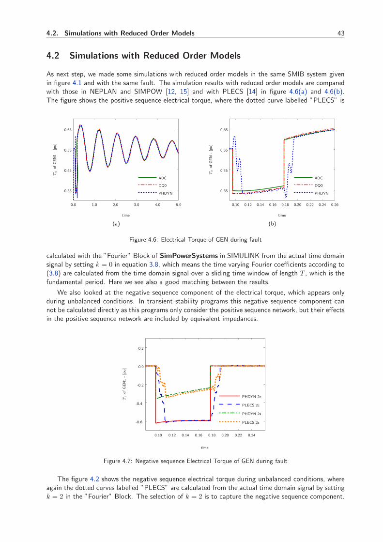
4.2. Simulations with Reduced Order Models 43
4.2 Simulations with Reduced Order Models
As next step, we made some simulations with reduced order models in the same SMIB system givenin figure 4.1 and with the same fault. The simulation results with reduced order models are comparedwith those in NEPLAN and SIMPOW [12, 15] and with PLECS [14] in figure 4.6(a) and 4.6(b).The figure shows the positive-sequence electrical torque, where the dotted curve labelled ”PLECS” is
time
Te
ofG
EN
1-
[pu]
0.0 1.0 2.0 3.0 4.0 5.0
0.35
0.45
0.55
0.65
ABC
DQ0
PHDYN
(a)
time
Te
ofG
EN
-[p
u]
0.10 0.12 0.14 0.16 0.18 0.20 0.22 0.24 0.26
0.35
0.45
0.55
0.65
ABC
DQ0
PHDYN
(b)
Figure 4.6: Electrical Torque of GEN during fault
calculated with the ”Fourier” Block of SimPowerSystems in SIMULINK from the actual time domainsignal by setting k = 0 in equation 3.8, which means the time varying Fourier coefficients according to(3.8) are calculated from the time domain signal over a sliding time window of length T , which is thefundamental period. Here we see also a good matching between the results.
We also looked at the negative sequence component of the electrical torque, which appears onlyduring unbalanced conditions. In transient stability programs this negative sequence component cannot be calculated directly as this programs only consider the positive sequence network, but their effectsin the positive sequence network are included by equivalent impedances.
time
Te
ofG
EN
1-
[pu]
0.10 0.12 0.14 0.16 0.18 0.20 0.22 0.24
-0.6
-0.4
-0.2
0.0
0.2
PHDYN 2c
PLECS 2c
PHDYN 2s
PLECS 2s
Figure 4.7: Negative sequence Electrical Torque of GEN during fault
The figure 4.2 shows the negative sequence electrical torque during unbalanced conditions, whereagain the dotted curves labelled ”PLECS” are calculated from the actual time domain signal by settingk = 2 in the ”Fourier” Block. The selection of k = 2 is to capture the negative sequence component.
4.3. Summary 44
With the use of phasor dynamic models with k = {0, 1, 2}, it was also possible to simulate the zero andnegative sequence quantities throughout in the system during unbalanced conditions in a systematicway. The simulation time with detailed models was 128 s and with reduced order phasor dynamicmodels 9 s.
4.3 Summary
In this chapter, we tried to verify our theoretical results from previous section by simulations. Thecomparison of the simulation times showed also the expected advantages and disadvantages of eachmodeling technique. Actually the appropriate selection of the modeling techniques is dependent on thenature of the study and the characteristics of the system.
But we should mention, that the test systems, we have selected in these studies, are small andcontain no controls. Our focus was more on the components and their models. Further investigationis needed with large networks and with more controls.

Chapter 5
Appendix
5.1 Fourier coefficients in real form
With Xk(t) = Xk,c(t) − j Xk,s(t) the equation (3.7) becomes
x(τ) =∞∑
k=0
(Xk,c(t) · cos(k ωs τ) + Xk,s(t) · sin(k ωs τ)) (-1)
the equation (3.8) becomes
Xk,c(t) =1T
t∫t−T
x(τ)· cos(k ωs τ) · dτ = 〈x〉k,c (t) (-2a)
Xk,s(t) =1T
t∫t−T
x(τ)· sin(k ωs τ) · dτ = 〈x〉k,s (t) (-2b)
the equation (3.9) becomes〈dtx〉k,c = dtXk,c + k · ωs · Xk,s (-3a)
〈dtx〉k,s = dtXk,s − k · ωs · Xk,c (-3b)
the equation (3.10) becomes
〈x · y〉k,c =12·
∞∑l=0
(Xk−l,c · Yl,c + Xk−l,s · Yl,s) (-4a)
〈x · y〉k,s =12·
∞∑l=0
(Xk−l,c · Yl,s + Xk−l,s · Yl,c) (-4b)
the equation (3.22) becomes
Xk,c = Fk,c (Xk,c, Xk,s, Yk,c, Yk,s) − k · ωs · Xk,s (-5)
Xk,s = Fk,s (Xk,c, Xk,s, Yk,c, Yk,s) + k · ωs · Xk,c
0 = Gk,c (Xk,c, Xk,s, Yk,c, Yk,s)0 = Gk,s (Xk,c, Xk,s, Yk,c, Yk,s)
45

5.2. TCSC - Harmonic Distortion Factor of Capacitor Voltage 46
5.2 TCSC - Harmonic Distortion Factor of Capacitor Voltage
with
XC = 1ωC , XL = ωL, ω0 = 1√
LC, η = ω0
ω
V sk = (−1)
k−12 · 4 |Il|
πk·⎛⎝ X2
C
2 (XC − XL)·⎛⎝sin
(σs(k+1)
2
)k + 1
+sin
(σs(k−1)
2
)k − 1
⎞⎠⎞⎠
+ (−1)k−12 · 4 |Il|
πk·(
X2C cos
(σs2
)cos
(k σs
2
) (k tan
(k σs
2
)− η tan(η σs
2
))(XC − XL) (η2 − k2)
)
V s1 =
|Il|π
(−XC +
X2C (sin (σs) + σs)(XC − XL)
+4 XC XL η2
(cos
(σs2
))2 (tan(
σs2
)− η tan(η σs
2
))(XC − XL) (η2 − 1)
)
ρk =V s
k
V s1

Bibliography
[1] I. Hiskens and M. Pai, “Hybrid systems view of power system modelling,” in Circuits and Systems,2000. Proceedings. ISCAS 2000 Geneva. The 2000 IEEE International Symposium on, vol. 2, 2000,pp. 228–231 vol.2.
[2] ——, “Trajectory sensitivity analysis of hybrid systems,” Circuits and Systems I: FundamentalTheory and Applications, IEEE Transactions on [see also Circuits and Systems I: Regular Papers,IEEE Transactions on], vol. 47, no. 2, pp. 204–220, 2000.
[3] T. Davis, “Umfpack version 4.0 user guide,” 2002.
[4] I. Hiskens and P. Sokolowski, “Systematic modeling and symbolically assisted simulation of powersystems,” Power Systems, IEEE Transactions on, vol. 16, no. 2, pp. 229–234, 2001.
[5] L. R. Petzold, “A description of dassl: A differential/algebraic system solver,” Scientific Comput-ing, eds. R.S. Stepleman et al., pp. 65–68, 1983.
[6] C. Gear, “The simultaneous numerical solution of differential-algebraic equations.” IEEE Trans.Circuit Theory, vol. CT-18, no. 1, pp. 89–95, 1971.
[7] P. Mattavelli, G. Verghese, and A. Stankovic, “Phasor dynamics of thyristor-controlled seriescapacitor systems,” Power Systems, IEEE Transactions on, vol. 12, no. 3, pp. 1259–1267, 1997.
[8] W. Hammer and G. Andersson, “Dynamic modeling of capacitor commutated converters,” inSEPOPE IX, Rio de Janeiro, Brazil, 2004.
[9] A. Stankovic and T. Aydin, “Analysis of asymmetrical faults in power systems using dynamicphasors,” Power Systems, IEEE Transactions on, vol. 15, no. 3, pp. 1062–1068, 2000.
[10] A. Stankovic, B. Lesieutre, and T. Aydin, “Applications of generalized averaging to synchronousand induction machines,” in North American Power Symposium, Boston, 1996, pp. 277–282.
[11] P. Kundur, N. J. Balu, and M. G. Lauby, Power system stability and control, ser. The EPRI powersystem engineering series. New York: McGraw-Hill, 1994.
[12] STRI, “Power system simulation and analysis software simpow, user manual, http://www.stri.se.”
[13] S. Sanders, J. Noworolski, X. Liu, and G. Verghese, “Generalized averaging method for powerconversion circuits,” Power Electronics, IEEE Transactions on, vol. 6, no. 2, pp. 251–259, 1991.
[14] Plexim, “Plecs user manual - high-speed simulations of electrical and power electronic circuitsunder matlab/simulink.”
[15] BCP, “Neplan software manual, http://www.neplan.ch.”
47