pdfs.semanticscholar.orgpdfs.semanticscholar.org/e36c/cf21710de71a6deee44... · multiscale model....

MULTISCALE MODEL. SIMUL. c© 2005 Society for Industrial and Applied MathematicsVol. 4, No. 2, pp. 490–530

A REVIEW OF IMAGE DENOISING ALGORITHMS, WITH A NEWONE∗

A. BUADES† , B. COLL† , AND J. M. MOREL‡

Abstract. The search for efficient image denoising methods is still a valid challenge at thecrossing of functional analysis and statistics. In spite of the sophistication of the recently proposedmethods, most algorithms have not yet attained a desirable level of applicability. All show an out-standing performance when the image model corresponds to the algorithm assumptions but fail ingeneral and create artifacts or remove image fine structures. The main focus of this paper is, first,to define a general mathematical and experimental methodology to compare and classify classicalimage denoising algorithms and, second, to propose a nonlocal means (NL-means) algorithm ad-dressing the preservation of structure in a digital image. The mathematical analysis is based on theanalysis of the “method noise,” defined as the difference between a digital image and its denoisedversion. The NL-means algorithm is proven to be asymptotically optimal under a generic statisticalimage model. The denoising performance of all considered methods are compared in four ways;mathematical: asymptotic order of magnitude of the method noise under regularity assumptions;perceptual-mathematical: the algorithms artifacts and their explanation as a violation of the imagemodel; quantitative experimental: by tables of L2 distances of the denoised version to the originalimage. The most powerful evaluation method seems, however, to be the visualization of the methodnoise on natural images. The more this method noise looks like a real white noise, the better themethod.

Key words. image restoration, nonparametric estimation, PDE smoothing filters, adaptivefilters, frequency domain filters

AMS subject classification. 62H35

DOI. 10.1137/040616024

1. Introduction.

1.1. Digital images and noise. The need for efficient image restoration meth-ods has grown with the massive production of digital images and movies of all kinds,often taken in poor conditions. No matter how good cameras are, an image improve-ment is always desirable to extend their range of action.

A digital image is generally encoded as a matrix of grey-level or color values. Inthe case of a movie, this matrix has three dimensions, the third one corresponding totime. Each pair (i, u(i)), where u(i) is the value at i, is called a pixel, short for “pictureelement.” In the case of grey-level images, i is a point on a two-dimensional (2D) gridand u(i) is a real value. In the case of classical color images, u(i) is a triplet of valuesfor the red, green, and blue components. All of what we shall say applies identicallyto movies, three-dimensional (3D) images, and color or multispectral images. For thesake of simplicity in notation and display of experiments, we shall here be contentwith rectangular 2D grey-level images.

∗Received by the editors September 30, 2004; accepted for publication (in revised form) Janu-ary 10, 2005; published electronically July 18, 2005.

http://www.siam.org/journals/mms/4-2/61602.html†Universitat de les Illes Balears, Anselm Turmeda, Ctra. Valldemossa Km. 7.5, 07122 Palma

de Mallorca, Spain ([email protected], [email protected]). These authors were supported by theMinisterio de Ciencia y Tecnologia under grant TIC2002-02172. During this work, the first authorhad a fellowship of the Govern de les Illes Balears for the realization of his Ph.D. thesis.

‡Centre de Mathematiques et Leurs Applications, ENS Cachan 61, Av du President Wilson 94235Cachan, France ([email protected]). This author was supported by the Centre Nationald’Etudes Spatiales (CNES), the Office of Naval Research under grant N00014-97-1-0839, the DirectionGenerale des Armements (DGA), and the Ministere de la Recherche et de la Technologie.

490

ON IMAGE DENOISING ALGORITHMS 491

The two main limitations in image accuracy are categorized as blur and noise.Blur is intrinsic to image acquisition systems, as digital images have a finite number ofsamples and must satisfy the Shannon–Nyquist sampling conditions [31]. The secondmain image perturbation is noise.

Each one of the pixel values u(i) is the result of a light intensity measurement,usually made by a charge coupled device (CCD) matrix coupled with a light focusingsystem. Each captor of the CCD is roughly a square in which the number of incomingphotons is being counted for a fixed period corresponding to the obturation time.When the light source is constant, the number of photons received by each pixelfluctuates around its average in accordance with the central limit theorem. In otherterms, one can expect fluctuations of order

√n for n incoming photons. In addition,

each captor, if not adequately cooled, receives heat spurious photons. The resultingperturbation is usually called “obscurity noise.” In a first rough approximation onecan write

v(i) = u(i) + n(i),

where i ∈ I, v(i) is the observed value, u(i) would be the “true” value at pixel i,namely the one which would be observed by averaging the photon counting on a longperiod of time, and n(i) is the noise perturbation. As indicated, the amount of noiseis signal-dependent; that is, n(i) is larger when u(i) is larger. In noise models, thenormalized values of n(i) and n(j) at different pixels are assumed to be independentrandom variables, and one talks about “white noise.”

1.2. Signal and noise ratios. A good quality photograph (for visual inspec-tion) has about 256 grey-level values, where 0 represents black and 255 representswhite. Measuring the amount of noise by its standard deviation, σ(n), one can definethe signal noise ratio (SNR) as

SNR =σ(u)

σ(n),

where σ(u) denotes the empirical standard deviation of u,

σ(u) =

(1

|I|∑i∈I

(u(i) − u)2

) 12

,

and u = 1|I|

∑i∈I u(i) is the average grey-level value. The standard deviation of the

noise can also be obtained as an empirical measurement or formally computed whenthe noise model and parameters are known. A good quality image has a standarddeviation of about 60.

The best way to test the effect of noise on a standard digital image is to add aGaussian white noise, in which case n(i) are independently and identically distributed(i.i.d.) Gaussian real variables. When σ(n) = 3, no visible alteration is usually ob-served. Thus, a 60

3 � 20 SNR is nearly invisible. Surprisingly enough, one can addwhite noise up to a 2

1 ratio and still see everything in a picture! This fact is il-lustrated in Figure 1 and constitutes a major enigma of human vision. It justifiesthe many attempts to define convincing denoising algorithms. As we shall see, theresults have been rather deceptive. Denoising algorithms see no difference betweensmall details and noise, and therefore they remove them. In many cases, they createnew distortions, and the researchers are so used to them that they have created a

492 A. BUADES, B. COLL, AND J. M. MOREL

Fig. 1. A digital image with standard deviation 55, the same with noise added (standarddeviation 3), the SNR therefore being equal to 18, and the same with SNR slightly larger than 2.In this second image, no alteration is visible. In the third, a conspicuous noise with standarddeviation 25 has been added, but, surprisingly enough, all details of the original image still arevisible.

taxonomy of denoising artifacts: “ringing,” “blur,” “staircase effect,” “checkerboardeffect,” “wavelet outliers,” etc.

This fact is not quite a surprise. Indeed, to the best of our knowledge, all denoisingalgorithms are based on

• a noise model;• a generic image smoothness model, local or global.

In experimental settings, the noise model is perfectly precise. So the weak point ofthe algorithms is the inadequacy of the image model. All of the methods assume thatthe noise is oscillatory and that the image is smooth or piecewise smooth. So they tryto separate the smooth or patchy part (the image) from the oscillatory one. Actually,many fine structures in images are as oscillatory as noise is; conversely, white noisehas low frequencies and therefore smooth components. Thus a separation methodbased on smoothness arguments only is hazardous.

1.3. The “method noise.” All denoising methods depend on a filtering pa-rameter h. This parameter measures the degree of filtering applied to the image. Formost methods, the parameter h depends on an estimation of the noise variance σ2.One can define the result of a denoising method Dh as a decomposition of any image vas

v = Dhv + n(Dh, v),(1.1)

where1. Dhv is more smooth than v,2. n(Dh, v) is the noise guessed by the method.

Now it is not enough to smooth v to ensure that n(Dh, v) will look like a noise.The more recent methods are actually not content with a smoothing but try to recoverlost information in n(Dh, v) [19, 25]. So the focus is on n(Dh, v).

Definition 1.1 (method noise). Let u be a (not necessarily noisy) image andDh a denoising operator depending on h. Then we define the method noise of u asthe image difference

n(Dh, u) = u−Dh(u).(1.2)

This method noise should be as similar to a white noise as possible. In addition,since we would like the original image u not to be altered by denoising methods, the


method noise should be as small as possible for the functions with the right regularity.According to the preceding discussion, four criteria can and will be taken into

account in the comparison of denoising methods:• A display of typical artifacts in denoised images.• A formal computation of the method noise on smooth images, evaluating how

small it is in accordance with image local smoothness.• A comparative display of the method noise of each method on real images

with σ = 2.5. We mentioned that a noise standard deviation smaller than 3 issubliminal, and it is expected that most digitization methods allow themselvesthis kind of noise.

• A classical comparison receipt based on noise simulation: it consists of takinga good quality image, adding Gaussian white noise with known σ, and thencomputing the best image recovered from the noisy one by each method. Atable of L2 distances from the restored to the original can be established. TheL2 distance does not provide a good quality assessment. However, it reflectswell the relative performances of algorithms.

On top of this, in two cases, a proof of asymptotic recovery of the image can beobtained by statistical arguments.

1.4. Which methods to compare. We had to make a selection of the denoisingmethods we wished to compare. Here a difficulty arises, as most original methods havecaused an abundant literature proposing many improvements. So we tried to get thebest available version, while keeping the simple and genuine character of the originalmethod: no hybrid method. So we shall analyze the following:

1. the Gaussian smoothing model (Gabor quoted in Lindenbaum, Fischer, andBruckstein [17]), where the smoothness of u is measured by the Dirichletintegral

∫|Du|2;

2. the anisotropic filtering model (Perona and Malik [27], Alvarez, Lions, andMorel [1]);

3. the Rudin–Osher–Fatemi total variation model [30] and two recently proposediterated total variation refinements [35, 25];

4. the Yaroslavsky neighborhood filters [41, 40] and an elegant variant, theSUSAN filter (Smith and Brady [33]);

5. the Wiener local empirical filter as implemented by Yaroslavsky [40];6. the translation invariant wavelet thresholding [8], a simple and performing

variant of the wavelet thresholding [10];7. DUDE, the discrete universal denoiser [24], and the UINTA, unsupervised

information-theoretic, adaptive filtering [3], two very recent new approaches;8. the nonlocal means (NL-means) algorithm, which we introduce here.

This last algorithm is given by a simple closed formula. Let u be defined in a boundeddomain Ω ⊂ R

2; then

NL(u)(x) =1

C(x)

∫e−

(Ga∗|u(x+.)−u(y+.)|2)(0)

h2 u(y) dy,

where x ∈ Ω, Ga is a Gaussian kernel of standard deviation a, h acts as a filtering

parameter, and C(x) =∫e−

(Ga∗|u(x+.)−u(z+.)|2)(0)

h2 dz is the normalizing factor. In orderto make clear the previous definition, we recall that

(Ga ∗ |u(x + .) − u(y + .)|2)(0) =

∫R2

Ga(t)|u(x + t) − u(y + t)|2dt.


This amounts to saying that NL(u)(x), the denoised value at x, is a mean of thevalues of all pixels whose Gaussian neighborhood looks like the neighborhood of x.

1.5. What is left. We do not draw into comparison the hybrid methods, inparticular the total variation + wavelets [7, 12, 18]. Such methods are significantimprovements of the simple methods but are impossible to draw into a benchmark:their efficiency depends a lot upon the choice of wavelet dictionaries and the kind ofimage.

Second, we do not draw into the comparison the method introduced recently byMeyer [22], whose aim it is to decompose the image into a BV part and a texturepart (the so called u + v methods), and even into three terms, namely u + v + w,where u is the BV part, v is the “texture” part belonging to the dual space of BV ,denoted by G, and w belongs to the Besov space B∞

−1,∞, a space characterized by thefact that the wavelet coefficients have a uniform bound. G is proposed by Meyer asthe right space to model oscillatory patterns such as textures. The main focus of thismethod is not yet denoising. Because of the different and more ambitious scopes of theMeyer method [2, 36, 26], which makes it parameter- and implementation-dependent,we could not draw it into the discussion. Last but not least, let us mention thebandlet [15] and curvelet [34] transforms for image analysis. These methods alsoare separation methods between the geometric part and the oscillatory part of theimage and intend to find an accurate and compressed version of the geometric part.Incidentally, they may be considered as denoising methods in geometric images, asthe oscillatory part then contains part of the noise. Those methods are closely relatedto the total variation method and to the wavelet thresholding, and we shall be contentwith those simpler representatives.

1.6. Plan of the paper. Section 2 computes formally the method noise for thebest elementary local smoothing methods, namely Gaussian smoothing, anisotropicsmoothing (mean curvature motion), total variation minimization, and the neighbor-hood filters. For all of them we prove or recall the asymptotic expansion of the filterat smooth points of the image and therefore obtain a formal expression of the methodnoise. This expression permits us to characterize places where the filter performs welland where it fails. In section 3, we treat the Wiener-like methods, which proceed bya soft or hard threshold on frequency or space-frequency coefficients. We examine inturn the Wiener–Fourier filter, the Yaroslavsky local adaptive discrete cosine trans-form (DCT)-based filters, and the wavelet threshold method. Of course, the Gaussiansmoothing belongs to both classes of filters. We also describe the universal denoiserDUDE, but we cannot draw it into the comparison, as its direct application to grey-level images is unpractical so far. (We discuss its feasibility.) Finally, we examinethe UINTA algorithms whose principles stand close to the NL-means algorithm. Insection 5, we introduce the NL-means filter. This method is not easily classified inthe preceding terminology, since it can work adaptively in a local or nonlocal way. Wefirst give a proof that this algorithm is asymptotically consistent (it gives back theconditional expectation of each pixel value given an observed neighborhood) underthe assumption that the image is a fairly general stationary random process. Theworks of Efros and Leung [13] and Levina [16] have shown that this assumption issound for images having enough samples in each texture patch. In section 6, we com-pare all algorithms from several points of view, do a performance classification, andexplain why the NL-means algorithm shares the consistency properties of most of theaforementioned algorithms.


2. Local smoothing filters. The original image u is defined in a boundeddomain Ω ⊂ R

2 and denoted by u(x) for x = (x, y) ∈ R2. This continuous image is

usually interpreted as the Shannon interpolation of a discrete grid of samples [31] andis therefore analytic. The distance between two consecutive samples will be denotedby ε.

The noise itself is a discrete phenomenon on the sampling grid. According tothe usual screen and printing visualization practice, we do not interpolate the noisesamples ni as a band limited function but rather as a piecewise constant function,constant on each pixel i and equal to ni.

We write |x| = (x2+y2)12 and x1.x2 = x1x2+y1y2 as the norm and scalar product

and denote the derivatives of u by ux = ∂u∂x , uy = ∂u

∂y , and uxy = ∂2u∂x∂y . The gradient

of u is written as Du = (ux, uy) and the Laplacian of u as Δu = uxx + uyy.

2.1. Gaussian smoothing. By Riesz’s theorem, image isotropic linear filteringboils down to a convolution of the image by a linear radial kernel. The smoothingrequirement is usually expressed by the positivity of the kernel. The paradigm of such

kernels is, of course, the Gaussian x → Gh(x) = 1(4πh2)e

− |x|24h2 . In that case, Gh has

standard deviation h, and the following theorem is easily seen.Theorem 2.1 (Gabor 1960). The image method noise of the convolution with a

Gaussian kernel Gh is

u−Gh ∗ u = −h2Δu + o(h2).

A similar result is actually valid for any positive radial kernel with boundedvariance, so one can keep the Gaussian example without loss of generality. Thepreceding estimate is valid if h is small enough. On the other hand, the noise reductionproperties depend upon the fact that the neighborhood involved in the smoothing islarge enough, so that the noise gets reduced by averaging. So in the following weassume that h = kε, where k stands for the number of samples of the function u andnoise n in an interval of length h. The spatial ratio k must be much larger than 1 toensure a noise reduction.

The effect of a Gaussian smoothing on the noise can be evaluated at a referencepixel i = 0. At this pixel,

Gh ∗ n(0) =∑i∈I

∫Pi

Gh(x)n(x)dx =∑i∈I

ε2Gh(i)ni,

where we recall that n(x) is being interpolated as a piecewise constant function, thePi square pixels centered in i have size ε2, and Gh(i) denotes the mean value of thefunction Gh on the pixel i.

Denoting by V ar(X) the variance of a random variable X, the additivity ofvariances of independent centered random variables yields

V ar(Gh ∗ n(0)) =∑i

ε4Gh(i)2σ2 � σ2ε2

∫Gh(x)2dx =

ε2σ2

8πh2.

So we have proved the following theorem.Theorem 2.2. Let n(x) be a piecewise constant white noise, with n(x) = ni on

each square pixel i. Assume that the ni are i.i.d. with zero mean and variance σ2.Then the “noise residue” after a Gaussian convolution of n by Gh satisfies

V ar(Gh ∗ n(0)) � ε2σ2

8πh2.


In other terms, the standard deviation of the noise, which can be interpreted as thenoise amplitude, is multiplied by ε

h√

8π.

Theorems 2.1 and 2.2 traduce the delicate equilibrium between noise reductionand image destruction by any linear smoothing. Denoising does not alter the imageat points where it is smooth at a scale h much larger than the sampling scale ε.The first theorem tells us that the method noise of the Gaussian denoising method iszero in harmonic parts of the image. A Gaussian convolution is optimal on harmonicfunctions and performs instead poorly on singular parts of u, namely edges or texture,where the Laplacian of the image is large. See Figure 3.

2.2. Anisotropic filters and curvature motion. The anisotropic filter (AF)attempts to avoid the blurring effect of the Gaussian by convolving the image u at xonly in the direction orthogonal to Du(x). The idea of such a filter goes back toPerona and Malik [27] and actually again to Gabor (quoted in Lindenbaum, Fischer,and Bruckstein [17]). Set

AFhu(x) =

∫Gh(t)u

(x + t

Du(x)⊥

|Du(x)|

)dt

for x such that Du(x) �= 0 and where (x, y)⊥ = (−y, x) and Gh(t) = 1√2πh

e−t2

2h2 is the

one-dimensional (1D) Gauss function with variance h2. At points where Du(x) = 0an isotropic Gaussian mean is usually applied, and the result of Theorem 2.1 holdsat those points. If one assumes that the original image u is twice continuously dif-ferentiable (C2) at x, the following theorem is easily shown by a second-order Taylorexpansion.

Theorem 2.3. The image method noise of an anisotropic filter AFh is

u(x) −AFhu(x) � −1

2h2D2u

(Du⊥

|Du| ,Du⊥

|Du|

)= −1

2h2|Du|curv(u)(x),

where the relation holds when Du(x) �= 0.

By curv(u)(x), we denote the curvature, i.e., the signed inverse of the radius ofcurvature of the level line passing by x. When Du(x) �= 0, this means that

curv(u) =uxxu

2y − 2uxyuxuy + uyyu

2x

(u2x + u2

y)32

.

This method noise is zero wherever u behaves locally like a one-variable function,u(x, y) = f(ax + by + c). In such a case, the level line of u is locally the straightline with equation ax + by + c = 0, and the gradient of f may instead be very large.In other terms, with anisotropic filtering, an edge can be maintained. On the otherhand, we have to evaluate the Gaussian noise reduction. This is easily done by a1D adaptation of Theorem 2.2. Notice that the noise on a grid is not isotropic; sothe Gaussian average when Du is parallel to one coordinate axis is made roughly on√

2 more samples than the Gaussian average in the diagonal direction.

Theorem 2.4. By anisotropic Gaussian smoothing, when ε is small enough withrespect to h, the noise residue satisfies

Var (AFh(n)) ≤ ε√2πh

σ2.


In other terms, the standard deviation of the noise n is multiplied by a factor at mostequal to ( ε√

2πh)1/2, this maximal value being attained in the diagonals.

Proof. Let L be the line x + tDu⊥(x)|Du(x)| passing by x, parameterized by t ∈ R,

and denote by Pi, i ∈ I, the pixels which meet L, n(i) the noise value, constant onpixel Pi, and εi the length of the intersection of L ∩ Pi. Denote by g(i) the average

of Gh(x + tDu⊥(x)|Du(x)| ) on L ∩ Pi. Then one has

AFhn(x) �∑i

εin(i)g(i).

The n(i) are i.i.d. with standard variation σ, and therefore

V ar(AFh(n)) =∑i

ε2iσ

2g(i)2 ≤ σ2 max(εi)∑i

εig(i)2.

This yields

Var (AFh(n)) ≤√

2εσ2

∫Gh(t)2dt =

ε√2πh

σ2.

There are many versions of AFh, all yielding an asymptotic estimate equivalentto the one in Theorem 2.3: the famous median filter [14], an inf-sup filter on segmentscentered at x [5], and the clever numerical implementation of the mean curvatureequation in [21]. So all of those filters have in common the good preservation of edges,but they perform poorly on flat regions and are worse there than a Gaussian blur.This fact derives from the comparison of the noise reduction estimates of Theorems2.1 and 2.4 and is experimentally patent in Figure 3.

2.3. Total variation. The total variation minimization was introduced by Ru-din and Osher [29] and Rudin, Osher, and Fatemi [30]. The original image u issupposed to have a simple geometric description, namely a set of connected sets, theobjects, along with their smooth contours, or edges. The image is smooth insidethe objects but with jumps across the boundaries. The functional space modelingthese properties is BV (Ω), the space of integrable functions with finite total variationTVΩ(u) =

∫|Du|, where Du is assumed to be a Radon measure. Given a noisy image

v(x), the above-mentioned authors proposed to recover the original image u(x) as thesolution of the constrained minimization problem

arg minu

TVΩ(u),(2.1)

subject to the noise constraints∫Ω

(u(x) − v(x))dx = 0 and

∫Ω

|u(x) − v(x)|2dx = σ2.

The solution u must be as regular as possible in the sense of the total variation,while the difference v(x)− u(x) is treated as an error, with a prescribed energy. Theconstraints prescribe the right mean and variance to u − v but do not ensure thatit is similar to a noise (see a thorough discussion in [22]). The preceding problem isnaturally linked to the unconstrained problem

arg minu

TVΩ(u) + λ

∫Ω

|v(x) − u(x)|2dx(2.2)


for a given Lagrange multiplier λ. The above functional is strictly convex and lowersemicontinuous with respect to the weak-star topology of BV . Therefore the minimumexists, is unique, and is computable (see, e.g., [6]). The parameter λ controls thetradeoff between the regularity and fidelity terms. As λ gets smaller the weight ofthe regularity term increases. Therefore λ is related to the degree of filtering of thesolution of the minimization problem. Let us denote by TVFλ(v) the solution ofproblem (2.2) for a given value of λ. The Euler–Lagrange equation associated withthe minimization problem is given by

(u(x) − v(x)) − 1

2λcurv(u)(x) = 0

(see [29]). Thus, we have the following theorem.Theorem 2.5. The image method noise of the total variation minimization (2.2)

is

u(x) − TVFλ(u)(x) = − 1

2λcurv(TVFλ(u))(x).

As in the anisotropic case, straight edges are maintained because of their smallcurvature. However, details and texture can be oversmoothed if λ is too small, as isshown in Figure 3.

2.4. Iterated total variation refinement. In the original total variation modelthe removed noise, v(x) − u(x), is treated as an error and is no longer studied. Inpractice, some structures and texture are present in this error. Several recent workshave tried to avoid this effect [35, 25].

2.4.1. The Tadmor–Nezzar–Vese approach. In [35], the authors have pro-posed to use the Rudin–Osher–Fatemi model iteratively. They decompose the noisyimage, v = u0 + n0, by the total variation model. So taking u0 to contain only ge-ometric information, they decompose by the very same model n0 = u1 + n1, whereu1 is assumed to be again a geometric part and n1 contains less geometric informa-tion than n0. Iterating this process, one obtains u = u0 + u1 + u2 + · · · + uk as arefined geometric part and nk as the noise residue. This strategy is in some senseclose to the matching pursuit methods [20]. Of course, the weight parameter in theRudin–Osher–Fatemi model has to grow at each iteration, and the authors propose ageometric series λ, 2λ, . . . , 2kλ. In that way, the extraction of the geometric part nk

becomes twice more taxing at each step. Then the new algorithm is as follows:1. Starting with an initial scale λ = λ0,

v = u0 + n0, [u0, n0] = arg minv=u+n

∫|Du| + λ0

∫|v(x) − u(x)|2dx.

2. Proceed with successive applications of the dyadic refinement nj = uj+1 +nj+1,

[uj+1, nj+1] = arg minnj=u+n

∫|Du| + λ02

j+1

∫|nj(x) − u(x)|2dx.

3. After k steps, we get the following hierarchical decomposition of v:

v = u0 + n0

= u0 + u1 + n1

= .....

= u0 + u1 + · · · + uk + nk.


The denoised image is given by the partial sum∑k

j=0 uj , and nk is the noise residue.This is a multilayered decomposition of v which lies in an intermediate scale of spaces,in between BV and L2. Some theoretical results on the convergence of this expansionare presented in [35].

2.4.2. The Osher et al. approach. The second algorithm due to Osher et al.[25] also consists of an iteration of the original model. The new algorithm is as follows:

1. First, solve the original total variation model

u1 = arg minu∈BV

{∫|∇u(x)|dx + λ

∫(v(x) − u(x))2dx

}

to obtain the decomposition v = u1 + n1.2. Perform a correction step to obtain

u2 = arg minu∈BV

{∫|∇u(x)|dx + λ

∫(v(x) + n1(x) − u(x))2dx

},

where n1 is the noise estimated by the first step. The correction step adds thisfirst estimate of the noise to the original image and raises the decompositionv + n1 = u2 + n2.

3. Iterate: compute uk+1 as a minimizer of the modified total variation mini-mization,

uk+1 = arg minu∈BV

{∫|∇u(x)|dx + λ

∫(v(x) + nk(x) − u(x))2dx

},

where

v + nk = uk+1 + nk+1.

Some results are presented in [25] which clarify the nature of the above sequence:• {uk}k converges monotonically in L2 to v, the noisy image, as k → ∞.• {uk}k approaches the noise-free image monotonically in the Bregman distance

associated with the BV seminorm, at least until ‖uk − u‖ ≤ σ2, where u isthe original image and σ is the standard deviation of the added noise.

These two results indicate how to stop the sequence and choose uk. It is enoughto proceed iteratively until the result gets noisier or the distance ‖uk−u‖2 gets smallerthan σ2. The new solution has more details preserved, as Figure 3 shows.

The above iterated denoising strategy being quite general, one can make thecomputations for a linear denoising operator T as well. In that case, this strategy

T (v + n1) = T (v) + T (n1)

amounts to saying that the first estimated noise n1 is filtered again and its smoothcomponents are added back to the original, which is in fact the Tadmor–Nezzar–Vesestrategy.

2.5. Neighborhood filters. The previous filters are based on a notion of spatialneighborhood or proximity. Neighborhood filters instead take into account grey-levelvalues to define neighboring pixels. In the simplest and more extreme case, the de-noised value at pixel i is an average of values at pixels which have a grey-level valueclose to u(i). The grey-level neighborhood is therefore

B(i, h) = {j ∈ I | u(i) − h < u(j) < u(i) + h}.


This is a fully nonlocal algorithm, since pixels belonging to the whole image are usedfor the estimation at pixel i. This algorithm can be written in a more continuousform,

NFhu(x) =1

C(x)

∫Ω

u(y)e−|u(y)−u(x)|2

h2 dy,

where Ω ⊂ R2 is an open and bounded set, and C(x) =

∫Ωe−

|u(y)−u(x)|2h2 dy is the

normalization factor. The first question to address here is the consistency of such afilter, namely, how close the denoised version is to the original when u is smooth.

Lemma 2.6. Suppose u is Lipschitz in Ω and h > 0; then C(x) ≥ O(h2).Proof. Given x,y ∈ Ω, by the mean value theorem, |u(x) − u(y)| ≤ K|x − y| for

some real constant K. Then C(x) =∫Ωe−

|u(y)−u(x)|2h2 dy ≥

∫B(x,h)

e−|u(y)−u(x)|2

h2 dy ≥e−K2

O(h2).Proposition 2.7 (method noise estimate). Suppose u is a Lipschitz bounded

function on Ω, where Ω is an open and bounded domain of R2. Then |u(x) −

NFhu(x)| = O(h√− log h) for h small, 0 < h < 1, x ∈ Ω.

Proof. Let x be a point of Ω, and for a given B and h, B, h ∈ R, consider the setDh = {y ∈ Ω | |u(y) − u(x)| ≤ Bh}. Then

|u(x) −NFhu(x)| ≤ 1

C

∫Dh

e−|u(y)−u(x)|2

h2 |u(y) − u(x)|dy

+1

C

∫Dc

h

e−|u(y)−u(x)|2

h2 |u(y) − u(x)|dy.

On one hand, considering that∫Dh

e−|u(y)−u(x)|2

h2 dy ≤ C(x) and |u(y)−u(x)| ≤ Bhfor y ∈ Dh one sees that the first term is bounded by Bh. On the other hand,

considering that e−|u(y)−u(x)|2

h2 ≤ e−B2

for y /∈ Dh,∫Dc

h|u(y) − u(x)|dy is bounded,

and by Lemma 2.6, C ≥ O(h2), one deduces that the second term has an order

O(h−2e−B2

). Finally, choosing B such that B2 = −3 log h yields

|u(x) −NFhu(x)| ≤ Bh + O(h−2e−B2

) = O(h√− log h) + O(h),

and so the method noise has order O(h√− log h).

The Yaroslavsky neighborhood filters [40, 41] consider mixed neighborhoodsB(i, h)∩Bρ(i), where Bρ(i) is a ball of center i and radius ρ. So the method takes anaverage of the values of pixels which are both close in grey-level and spatial distance.This filter can be easily written in a continuous form as

YNFh,ρ(x) =1

C(x)

∫Bρ(x)

u(y)e−|u(y)−u(x)|2

h2 dy,

where C(x) =∫Bρ(x)

e−|u(y)−u(x)|2

h2 dy is the normalization factor. In [33] the authors

present a similar approach where they do not consider a ball of radius ρ but weighthe distance to the central pixel, obtaining the following close formula:

1

C(x)

∫u(y)e

− |y−x|2ρ2 e−

|u(y)−u(x)|2h2 dy,

where C(x) =∫e− |y−x|2

ρ2 e−|u(y)−u(x)|2

h2 dy is the normalization factor.


First, we study the method noise of the YNFh,ρ in the 1D case. In that case,u denotes a 1D signal.

Theorem 2.8. Suppose u ∈ C2((a, b)), a, b ∈ R. Then, for 0 < ρ � h andh → 0,

u(s) − YNFh,ρu(s) � −ρ2

2f(ρh|u′(s)|

)u′′(s),

where

f(t) =13 − 3

5 t2

1 − 13 t

2.

Proof. Let s ∈ (a, b) and h, ρ ∈ R+. Then

u(s) − YNFh,ρ(s) = − 1∫ ρ

−ρe−

(u(s+t)−u(s))2

h2 dt

∫ ρ

−ρ

(u(s + t) − u(s))e−(u(s+t)−u(s))2

h2 dt.

If we take the Taylor expansion of u(s+ t) and the exponential function e−x2

and weintegrate, then we obtain that

u(s) − YNFh,ρ(s) � −ρ3u′′

3 − 3ρ5u′2u′′

5h2

2h− 2ρ3u′2

3h2

for ρ small enough. The method noise follows from the above expression.

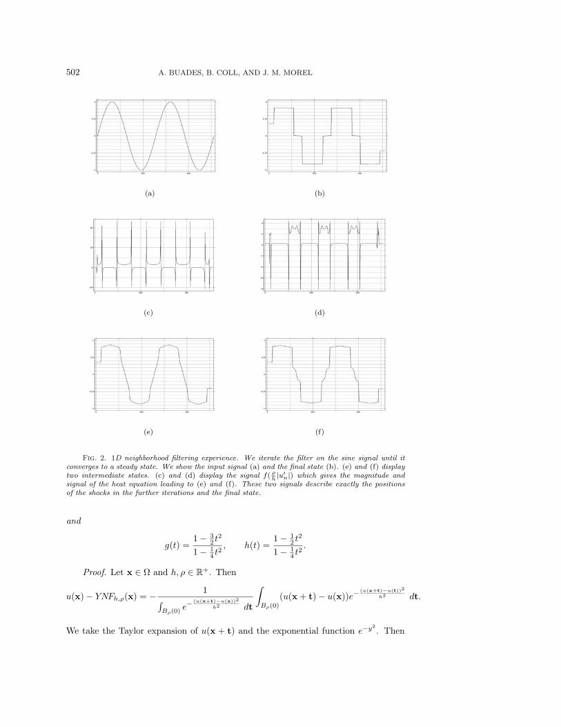
The previous result shows that the neighborhood filtering method noise is pro-portional to the second derivative of the signal. That is, it behaves like a weightedheat equation. The function f gives the sign and the magnitude of this heat equation.Where the function f takes positive values, the method noise behaves as a pure heatequation, while where it takes negative values, the method noise behaves as a reverseheat equation. The zeros and the discontinuity points of f represent the singularpoints where the behavior of the method changes. The magnitude of this change ismuch larger near the discontinuities of f producing an amplified shock effect. Figure 2displays one experiment with the 1D neighborhood filter. We iterate the algorithm ona sine signal and illustrate the shock effect. For the two intermediate iterations un+1,we display the signal f( ρ

h |u′n|) which gives the sign and magnitude of the heat equa-

tion at each point. We can see that the positions of the discontinuities of f( ρh |u′

n|)describe exactly the positions of the shocks in the further iterations and the finalstate. These two examples corroborate Theorem 2.8 and show how the function ftotally characterizes the performance of the 1D neighborhood filter.

Next we give the analogous result for 2D images.

Theorem 2.9. Suppose u ∈ C2(Ω), Ω ⊂ R2. Then, for 0 < ρ � h and h → 0,

u(x) − YNFh,ρ(x) � −ρ2

8

(g(ρh|Du|

)uηη + h

(ρh|Du|

)uξξ

),

where

uηη = D2u

(Du

|Du| ,Du

|Du|

), uξξ = D2u

(Du⊥

|Du| ,Du⊥

|Du|

)


(a) (b)

(c) (d)

(e) (f)

Fig. 2. 1D neighborhood filtering experience. We iterate the filter on the sine signal until itconverges to a steady state. We show the input signal (a) and the final state (b). (e) and (f) displaytwo intermediate states. (c) and (d) display the signal f( ρ

h|u′

n|) which gives the magnitude andsignal of the heat equation leading to (e) and (f). These two signals describe exactly the positionsof the shocks in the further iterations and the final state.

and

g(t) =1 − 3

2 t2

1 − 14 t

2, h(t) =

1 − 12 t

2

1 − 14 t

2.

Proof. Let x ∈ Ω and h, ρ ∈ R+. Then

u(x) − YNFh,ρ(x) = − 1∫Bρ(0)

e−(u(x+t)−u(x))2

h2 dt

∫Bρ(0)

(u(x + t) − u(x))e−(u(x+t)−u(t))2

h2 dt.

We take the Taylor expansion of u(x + t) and the exponential function e−y2

. Then


we take polar coordinates and integrate, obtaining

u(x) − YNFh,ρ(x) � 1

πρ2 − ρ4π4h2 (u2

x + u2y)

(πρ4

8Δu− πρ6

16h2

(u2xuxx + u2

yuxx

+ u2xuyy + u2

xuxx

)− πρ6

8h2(u2

xuxx + 2uxuyuxy + u2yuyy)

)

for ρ small enough. By grouping the terms of above expression, we get the desiredresult.

The neighborhood filtering method noise can be written as the sum of a diffusionterm in the tangent direction uξξ, plus a diffusion term in the normal direction, uηη.The sign and the magnitude of both diffusions depend on the sign and the magnitudeof the functions g and h. Both functions can take positive and negative values.Therefore, both diffusions can appear as a directional heat equation or directionalreverse heat equation, depending on the value of the gradient. As in the 1D case,the algorithm performs like a filtering/enhancing algorithm, depending on the valueof the gradient. If B1 =

√2/√

3 and B2 =√

2, respectively, denote the zeros of thefunctions g and h, we can distinguish the following cases:

• When 0 < |Du| < B2hρ the algorithm behaves like the Perona–Malik fil-

ter [27]. In a first step, a heat equation is applied, but when |Du| > B1hρ the

normal diffusion turns into a reverse diffusion, enhancing the edges, while thetangent diffusion stays positive.

• When |Du| > B2hρ the algorithm differs from the Perona–Malik filter. A heat

equation or a reverse heat equation is applied, depending on the value of thegradient. The change of behavior between these two dynamics is marked byan asymptotical discontinuity leading to an amplified shock effect.

Fig. 3. Denoising experience on a natural image. From left to right and from top to bottom:noisy image (standard deviation 20), Gaussian convolution, anisotropic filter, total variation min-imization, Tadmor–Nezzar–Vese iterated total variation, Osher et al. iterated total variation, andthe Yaroslavsky neighborhood filter.

3. Frequency domain filters. Let u be the original image defined on the grid I.The image is supposed to be modified by the addition of a signal independent whitenoise N . N is a random process where N(i) are i.i.d. with zero mean and have constant


variance σ2. The resulting noisy process depends on the random noise component,and therefore it is modeled as a random field V ,

V (i) = u(i) + N(i).(3.1)

Given a noise observation n(i), v(i) denotes the observed noisy image,

v(i) = u(i) + n(i).(3.2)

Let B = {gα}α∈A be an orthogonal basis of R|I|. The noisy process is transformed

as

VB(α) = uB(α) + NB(α),(3.3)

where

VB(α) = 〈V, gα〉, uB(α) = 〈u, gα〉, NB(α) = 〈N, gα〉

are the scalar products of V , u, and N with gα ∈ B. The noise coefficients NB(α)remain uncorrelated and with zero mean, but the variances are multiplied by ‖gα‖2:

E[NB(α)NB(β)] =∑

m,n∈I

gα(m)gβ(n)E[N(m)N(n)]

= 〈gα, gβ〉σ2 = σ2‖gα‖2δ[α− β].

Frequency domain filters are applied independently to every transform coefficientVB(α), and then the solution is estimated by the inverse transform of the new co-efficients. Noisy coefficients VB(α) are modified to a(α)VB(α). This is a nonlinearalgorithm because a(α) depends on the value VB(α). The inverse transform yields theestimate

U = DV =∑α∈A

a(α) VB(α) gα.(3.4)

D is also called a diagonal operator. Let us look for the frequency domain filter Dwhich minimizes a certain estimation error. This error is based on the square Eu-clidean distance, and it is averaged over the noise distribution.

Definition 3.1. Let u be the original image, N be a white noise, and V = u+N .Let D be a frequency domain filter. Define the risk of D as

r(D,u) = E{‖u−DV ‖2},(3.5)

where the expectation is taken over the noise distribution.The following theorem, which is easily proved, gives the diagonal operator Dinf

that minimizes the risk,

Dinf = arg minD

r(D,u).

Theorem 3.2. The operator Dinf which minimizes the risk is given by the family{a(α)}α, where

a(α) =|uB(α)|2

|uB(α)|2 + ‖gα‖2σ2,(3.6)


and the corresponding risk is

rinf (u) =∑s∈S

‖gα‖4 |uB(α)|2σ2

|uB(α)|2 + ‖gα‖2σ2.(3.7)

The previous optimal operator attenuates all noisy coefficients in order to mini-mize the risk. If one restricts a(α) to be 0 or 1, one gets a projection operator. Inthat case, a subset of coefficients is kept, and the rest gets canceled. The projectionoperator that minimizes the risk r(D,u) is obtained by the family {a(α)}α, where

a(α) =

{1 |uB(α)|2 ≥ ‖gα‖2σ2,

0 otherwise

and the corresponding risk is

rp(u) =∑

‖gα‖2 min(|uB(α)|2, ‖gα‖2σ2).

Note that both filters are ideal operators because they depend on the coefficientsuB(α) of the original image, which are not known. We call, as classical, Fourier–Wiener filter the optimal operator (3.6) where B is a Fourier basis. This is an idealfilter, since it uses the (unknown) Fourier transform of the original image. By the useof the Fourier basis (see Figure 4), global image characteristics may prevail over localones and create spurious periodic patterns. To avoid this effect, the basis must takeinto account more local features, as the wavelet and local DCT transforms do. Thesearch for the ideal basis associated with each image is still open. At the moment,the way seems to be a dictionary of basis instead of one single basis [19].

Fig. 4. Fourier–Wiener filter experiment. Top left: Degraded image by an additive white noiseof σ = 15. Top right: Fourier–Wiener filter solution. Bottom: Zoom on three different zones ofthe solution. The image is filtered as a whole, and therefore a uniform texture is spread all over theimage.


3.1. Local adaptive filters in transform domain. The local adaptive filtershave been introduced by Yaroslavsky and Eden [41] and Yaroslavsky [42]. In thiscase, the noisy image is analyzed in a moving window, and in each position of thewindow its spectrum is computed and modified. Finally, an inverse transform is usedto estimate only the signal value in the central pixel of the window.

Let i ∈ I be a pixel and W = W (i) a window centered in i. Then the DCT trans-form of W is computed and modified. The original image coefficients of W , uB,W (α),are estimated, and the optimal attenuation of Theorem 3.2 is applied. Finally, onlythe center pixel of the restored window is used. This method is called the empiricalWiener filter. In order to approximate uB,W (α), one can take averages on the additivenoise model, that is,

E|VB,W (α)|2 = |uB,W (α)|2 + σ2‖gα‖2.

Denoting by μ = σ‖gα‖, the unknown original coefficients can be written as

|uB,W (α)|2 = E|VB,W (α)|2 − μ2.

The observed coefficients |vB,W (α)|2 are used to approximate E|VB,W (α)|2, and theestimated original coefficients are replaced in the optimal attenuation, leading to thefamily {a(α)}α, where

a(α) = max

{0,

|vB,W (α)|2 − μ2

|vB,W (α)|2

}.

Denote by EWFμ(i) the filter given by the previous family of coefficients. The methodnoise of the EWFμ(i) is easily computed, as proved in the following theorem.

Theorem 3.3. Let u be an image defined in a grid I, and let i ∈ I be a pixel.Let W = W (i) be a window centered in the pixel i. Then the method noise of theEWFμ(i) is given by

u(i) − EWFμ(i) =∑α∈Λ

vB,W(α) gα(i) +∑α/∈Λ

μ2

|vB,W(α)|2 vB,W(α) gα(i),

where Λ = {α | |vB,W(α)| < μ}.The presence of an edge in the window W will produce a great number of large

coefficients, and, as a consequence, the cancelation of these coefficients will produceoscillations. Then spurious cosines will also appear in the image under the form ofchessboard patterns; see Figure 5.

3.2. Wavelet thresholding. Let B = {gα}α∈A be an orthonormal basis ofwavelets [20]. Let us discuss two procedures modifying the noisy coefficients, calledwavelet thresholding methods (Donoho and Johnstone [10]). The first procedure is aprojection operator which approximates the ideal projection (3.6). It is called a hardthresholding and cancels coefficients smaller than a certain threshold μ,

a(α) =

{1 |vB(α)| > μ,

0 otherwise.

Let us denote this operator by HWTμ(v). This procedure is based on the idea that theimage is represented with large wavelet coefficients, which are kept, whereas the noise


is distributed across small coefficients, which are canceled. The performance of themethod depends on the capacity of approximating u by a small set of large coefficients.Wavelets are, for example, an adapted representation for smooth functions.

Theorem 3.4. Let u be an image defined in a grid I. The method noise of ahard thresholding HWTμ(u) is

u−HWTμ(u) =∑

{α||uB(α)|<μ}uB(α)gα.

Unfortunately, edges lead to a great amount of wavelet coefficients lower thanthe threshold but not zero. The cancelation of these wavelet coefficients causes smalloscillations near the edges, i.e., a Gibbs-like phenomenon. Spurious wavelets can alsobe seen in the restored image due to the cancelation of small coefficients; see Figure 5.This artifact will be called wavelet outliers, as it is introduced in [11]. Donoho [9]showed that these effects can be partially avoided with the use of a soft thresholding,

a(α) =

{vB(α)−sgn(vB(α))μ

vB(α) , |vB(α)| ≥ μ,

0 otherwise,

which will be denoted by SWTμ(v). The continuity of the soft thresholding operatorbetter preserves the structure of the wavelet coefficients, reducing the oscillations neardiscontinuities. Note that a soft thresholding attenuates all coefficients in order toreduce the noise, as an ideal operator does. As we shall see at the end of this paper,the L2 norm of the method noise is lessened when replacing the hard threshold by asoft threshold. See Figures 5 and 15 for a comparison of both method noises.

Theorem 3.5. Let u be an image defined in a grid I. The method noise of a softthresholding SWTμ(u) is

u− SWTμ(u) =∑

{α||uB(α)|<μ}uB(α)gα + μ

∑{α||uB(α)|>μ}

sgn(uB(α)) gα.

A simple example can show how to fix the threshold μ. Suppose the originalimage u is zero; then vB(α) = nB(α), and therefore the threshold μ must be takenover the maximum of noise coefficients to ensure their suppression and the recoveryof the original image. It can be shown that the maximum amplitude of a white noisehas a high probability of being smaller than σ

√2 log |I|. It can be proved that the

risk of a wavelet thresholding with the threshold μ = σ√

2 log |I| is near the risk rpof the optimal projection; see [10, 20].

Theorem 3.6. The risk rt(u) of a hard or soft thresholding with the thresholdμ = σ

√2 log |I| is such that for all |I| ≥ 4

rt(u) ≤ (2 log |I| + 1)(σ2 + rp(u)).(3.8)

The factor 2 log |I| is optimal among all the diagonal operators in B, that is,

lim|I|−>∞

infD∈DB

supu∈R|I|

E{‖u−DV ‖2}σ2 + rp(u)

1

2 log |I| = 1.(3.9)

In practice the optimal threshold μ is very high and cancels too many coefficientsnot produced by the noise. A threshold lower than the optimal is used in the exper-iments and produces much better results; see Figure 5. For a hard thresholding thethreshold is fixed to 3 ∗ σ. For a soft thresholding this threshold still is too high; it isbetter fixed at 3

2σ.


3.3. Translation invariant wavelet thresholding. Coifman and Donoho [8]improved the wavelet thresholding methods by averaging the estimation of all trans-lations of the degraded signal. Calling vp(i) the translated signal v(i−p), the waveletcoefficients of the original and translated signals can be very different, and they arenot related by a simple translation or permutation,

vpB(α) = 〈v(n− p), gα(n)〉 = 〈v(n), gα(n + p)〉.

The vectors gα(n+ p) are not in general in the basis B = {gα}α∈A, and therefore theestimation of the translated signal is not related to the estimation of v. This newalgorithm yields an estimate up for every translated vp of the original image,

up = Dvp =∑α∈A

a(α)vpB(α)gα.(3.10)

The translation invariant thresholding is obtained by averaging all these estimatorsafter a translation in the inverse sense,

1

|I|∑p∈I

up(i + p),(3.11)

and will be denoted by TIWT (v).The Gibbs effect is considerably reduced by the translation invariant wavelet

thresholding (see Figure 5), because the average of different estimations of the imagereduces the oscillations. This is therefore the version we shall use in the comparisonsection. Recently, Durand and Nikolova [11] have actually proposed an efficient vari-ational method finding the best compromise to avoid the three common artifacts intotal variation methods and wavelet thresholding, namely the staircasing, the Gibbseffect, and the wavelet outliers. Unfortunately, we could not draw the method intothe comparison.

Fig. 5. Denoising experiment on a natural image. From left to right and from top to bottom:noisy image (standard deviation 20), Fourier–Wiener filter (ideal filter), the DCT empirical Wienerfilter, the wavelet hard thresholding, the soft wavelet thresholding, and the translation invariantwavelet hard thresholding.


4. Statistical neighborhood approaches. The methods we are going to con-sider are very recent attempts to take advantage of an image model learned from theimage itself. More specifically, these denoising methods attempt to learn the statisti-cal relationship between the image values in a window around a pixel and the pixelvalue at the window center.

4.1. DUDE, a universal denoiser. The recent work by Weissman et al. [38]has led to the proposition of a “universal denoiser” for digital images. The authorsassume that the noise model is fully known, namely the probability transition matrixΠ(a, b), where a, b ∈ A, the finite alphabet of all possible values for the image. Inorder to fix ideas, we shall assume as in the rest of this paper that the noise is additive

Gaussian, in which case one simply has Π(a, b) = 1√2πσ

e−(a−b)2

2σ2 for the probability

of observing b when the real value was a. The authors also fix an error cost Λ(a, b)which, to fix ideas, we can take to be a quadratic function Λ(a, b) = (a− b)2, namely,the cost of mistaking a for b.

The authors fix a neighborhood shape, say, a square discrete window deprived ofits center i, Ni = Ni \ {i} around each pixel i. Then the question is, Once the imagehas been observed in the window Ni, what is the best estimate we can make from theobservation of the full image?

The authors propose the following algorithm:• Compute, for each possible value b of u(i), the number of windows Nj in the

image such that the restrictions of u to Nj and Ni coincide and the observedvalue at the pixel j is b. This number is called m(b,Ni), and the line vector(m(b,Ni))b∈A is denoted by m(Ni).

• Then compute the denoised value of u at i as

u(i) = arg minb∈A

m(Ni)Π−1(Λb ⊗ Πu(i)),

where w ⊗ v = (w(b)v(b)) denotes the vector obtained by multiplying eachcomponent of u by each component of v, u(i) is the observed value at i, andwe denote by Xa the a-column of a matrix X.

The authors prove that this denoiser is universal in the sense “of asymptoticallyachieving, without access to any information on the statistics of the clean signal,the same performance as the best denoiser that does have access to this information.”In [24] the authors present an implementation valid for binary images with an impulsenoise, with excellent results. The reason of these limitations in implementation areclear: First, the matrix Π is of very low dimension and invertible for impulse noise. Ifinstead we consider as above a Gaussian noise, then the application of Π−1 amountsto deconvolving a signal by a Gaussian, which is a rather ill-conditioned method.All the same, it is doable, while the computation of m certainly is not for a largealphabet, such as the one involved in grey-tone images (256 values). Even supposingthat the learning window Ni has the minimal possible size of 9, the number of possiblesuch windows is about 2569, which turns out to be much larger than the number ofobservable windows in an image (whose typical size amounts to 106 pixels). Actually,the number of samples can be made significantly smaller by quantizing the grey-levelimage and by noting that the window samples are clustered. Anyway, the directobservation of the number m(Ni) in an image is almost hopeless, particularly if it iscorrupted by noise.

4.2. The UINTA algorithm. Awate and Whitaker [3] have proposed a methodwhose principles stand close to the NL-means algorithm, since, as in DUDE, the


method involves comparison between subwindows to estimate a restored value. Theobjective of the algorithm “UINTA, for unsupervised information-theoretic, adaptivefiltering” is to denoise the image, decreasing the randomness of the image. Thealgorithm proceeds as follows:

• Assume that the (2d+ 1)× (2d+ 1) windows in the image are realizations ofa random vector Z. The probability distribution function of Z is estimatedfrom the samples in the image,

p(z) =1

|A|∑zi∈A

Gσ(z − zi),

where z ∈ R(2d+1)×(2d+1), Gσ is the Gaussian density function in dimension n

with variance σ2,

Gσ(x) =1

(2π)n2 σ

e−‖x‖2

σ2 ,

and A is a random subset of windows in the image.• Then the authors propose an iterative method which minimizes the entropy

of the density distribution,

Ep log p(Z) = −∫

p(z) log p(z)dz.

This minimization is achieved by a gradient descent algorithm of the previousenergy function.

The denoising effect of this algorithm can be understood, as it forces the proba-bility density to concentrate. Thus, groups of similar windows tend to assume a moreand more similar configuration which is less noisy. The differences of this algorithmwith NL-means are patent, however. This algorithm creates a global interaction be-tween all windows. In particular, it tends to favor big groups of similar windows andto remove small groups. To that extent, it is a global homogenization process and isquite valid if the image consists of a periodic or quasi-periodic texture, as is patentin the successful experiments shown in this paper. The spirit of this method is todefine a new, information theoretically oriented scale space. In that sense, the gradi-ent descent must be stopped before a steady state. The time at which the process isstopped gives us the scale of randomness of the filtered image.

5. NL-means algorithm. The local smoothing methods and the frequency do-main filters aim at a noise reduction and at a reconstruction of the main geometricalconfigurations but not at the preservation of the fine structure, details, and texture.Due to the regularity assumptions on the original image of previous methods, detailsand fine structures are smoothed out because they behave in all functional aspectsas noise. The NL-means algorithm we shall now discuss tries to take advantage ofthe high degree of redundancy of any natural image. By this, we simply mean thatevery small window in a natural image has many similar windows in the same image.This fact is patent for windows close by, at one pixel distance, and in that case wego back to a local regularity assumption. Now in a very general sense inspired by theneighborhood filters, one can define as “neighborhood of a pixel i” any set of pixels jin the image such that a window around j looks like a window around i. All pixelsin that neighborhood can be used for predicting the value at i, as was first shownin [13] for 2D images. This first work has inspired many variants for the restoration


of various digital objects, in particular 3D surfaces [32]. The fact that such a self-similarity exists is a regularity assumption, actually more general and more accuratethan all regularity assumptions we have considered in section 2. It also generalizes aperiodicity assumption of the image.

Let v be the noisy image observation defined on a bounded domain Ω ⊂ R2, and

let x ∈ Ω. The NL-means algorithm estimates the value of x as an average of thevalues of all the pixels whose Gaussian neighborhood looks like the neighborhood of x,

NL(v)(x) =1

C(x)

∫Ω

e−(Ga∗|v(x+.)−v(y+.)|2)(0)

h2 v(y) dy,

where Ga is a Gaussian kernel with standard deviation a, h acts as a filtering pa-

rameter, and C(x) =∫Ωe−

(Ga∗|v(x+.)−v(z+.)|2)(0)

h2 dz is the normalizing factor. We recallthat

(Ga ∗ |v(x + .) − v(y + .)|2)(0) =

∫R2

Ga(t)|v(x + t) − v(y + t)|2dt.

Since we are considering images defined on a discrete grid I, we shall give a discretedescription of the NL-means algorithm and some consistency results. This simple andgeneric algorithm and its application to the improvement of the performance of digitalcameras are the object of an European patent application [4].

5.1. Description. Given a discrete noisy image v = {v(i) | i ∈ I}, the estimatedvalue NL(v)(i) is computed as a weighted average of all the pixels in the image,

NL(v)(i) =∑j∈I

w(i, j)v(j),

where the weights {w(i, j)}j depend on the similarity between the pixels i and j andsatisfy the usual conditions 0 ≤ w(i, j) ≤ 1 and

∑j w(i, j) = 1.

In order to compute the similarity between the image pixels, we define a neigh-borhood system on I.

Definition 5.1 (neighborhoods). A neighborhood system on I is a family N ={Ni}i∈I of subsets of I such that for all i ∈ I,

(i) i ∈ Ni,(ii) j ∈ Ni ⇒ i ∈ Nj.

The subset Ni is called the neighborhood or the similarity window of i. We set Ni =Ni \ {i}.

The similarity windows can have different sizes and shapes to better adapt to theimage. For simplicity we will use square windows of fixed size. The restriction of v toa neighborhood Ni will be denoted by v(Ni):

v(Ni) = (v(j), j ∈ Ni).

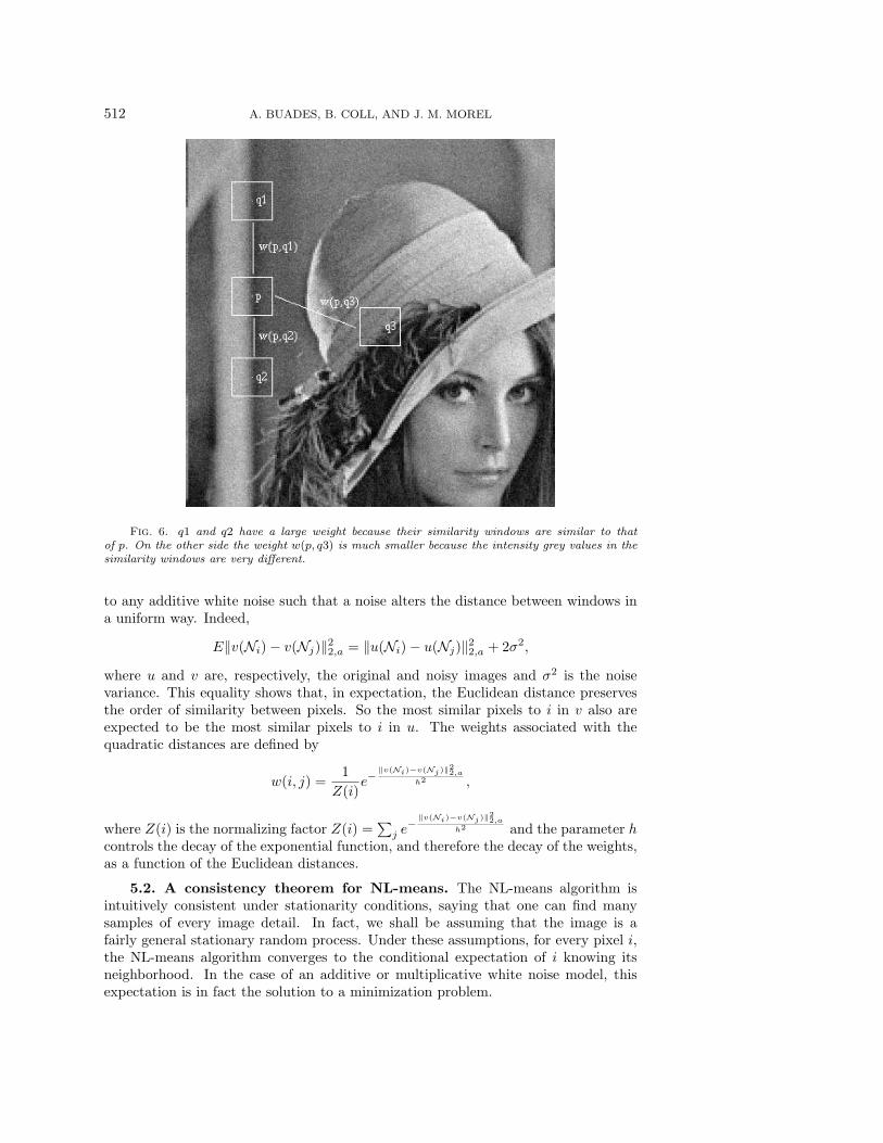
The similarity between two pixels i and j will depend on the similarity of theintensity grey-level vectors v(Ni) and v(Nj). The pixels with a similar grey-levelneighborhood to v(Ni) will have larger weights on the average; see Figure 6.

In order to compute the similarity of the intensity grey-level vectors v(Ni) andv(Nj), one can compute a Gaussian weighted Euclidean distance, ‖v(Ni)−v(Nj)‖2

2,a.Efros and Leung [13] showed that the L2 distance is a reliable measure for the compar-ison of image windows in a texture patch. Now this measure is so much more adapted


Fig. 6. q1 and q2 have a large weight because their similarity windows are similar to thatof p. On the other side the weight w(p, q3) is much smaller because the intensity grey values in thesimilarity windows are very different.

to any additive white noise such that a noise alters the distance between windows ina uniform way. Indeed,

E‖v(Ni) − v(Nj)‖22,a = ‖u(Ni) − u(Nj)‖2

2,a + 2σ2,

where u and v are, respectively, the original and noisy images and σ2 is the noisevariance. This equality shows that, in expectation, the Euclidean distance preservesthe order of similarity between pixels. So the most similar pixels to i in v also areexpected to be the most similar pixels to i in u. The weights associated with thequadratic distances are defined by

w(i, j) =1

Z(i)e−

‖v(Ni)−v(Nj)‖22,a

h2 ,

where Z(i) is the normalizing factor Z(i) =∑

j e−

‖v(Ni)−v(Nj)‖22,a

h2 and the parameter hcontrols the decay of the exponential function, and therefore the decay of the weights,as a function of the Euclidean distances.

5.2. A consistency theorem for NL-means. The NL-means algorithm isintuitively consistent under stationarity conditions, saying that one can find manysamples of every image detail. In fact, we shall be assuming that the image is afairly general stationary random process. Under these assumptions, for every pixel i,the NL-means algorithm converges to the conditional expectation of i knowing itsneighborhood. In the case of an additive or multiplicative white noise model, thisexpectation is in fact the solution to a minimization problem.


Let X and Y denote two random vectors with values on Rp and R, respectively.

Let fX , fY denote the probability distribution functions of X, Y , and let fXY denotethe joint probability distribution function of X and Y . Let us recall briefly thedefinition of the conditional expectation.

Definition 5.2.

(i) Define the probability distribution function of Y conditioned to X as

f(y | x) =

{fXY (x,y)fX(x) if fX(x) > 0,

0 otherwise

for all x ∈ Rp and y ∈ R.

(ii) Define the conditional expectation of Y given {X = x} as the expectationwith respect to the conditional distribution f(y | x),

E[Y | X = x] =

∫y f(y | x) dy,

for all x ∈ Rp.

The conditional expectation is a function of X, and therefore a new randomvariable g(X), which is denoted by E[Y | X].

Now let V be a random field and N a neighborhood system on I. Let Z denotethe sequence of random variables Zi = {Yi, Xi}i∈I , where Yi = V (i) is real valuedand Xi = V (Ni) is R

p valued. Recall that Ni = Ni \ {i}.Let us restrict Z to the n first elements {Yi, Xi}ni=1. Let us define the function

rn(x),

rn(x) = Rn(x)/fn(x),(5.1)

where

fn(x) =1

nhp

n∑i=1

K

(Xi − x

h

), Rn(x) =

1

nhp

n∑i=1

φ(Yi)K

(Xi − x

h

),(5.2)

φ is an integrable real valued function, K is a nonnegative kernel, and x ∈ Rp.

Let X and Y be distributed as X1 and Y1. Under this form the NL-meansalgorithm can be seen as an instance for the exponential operator of the Nadaraya–Watson estimator [23, 37]. This is an estimator of the conditional expectation r(x) =E[φ(Y ) | X = x]. Some definitions are needed for the statement of the main result.

Definition 5.3. A stochastic process {Zt | t = 1, 2, . . .}, with Zt defined onsome probability space (Ω,A,P), is said to be (strict-sense) stationary if for anyfinite partition {t1, t2, . . . , tn} the joint distributions Ft1,t2,...,tn(x1, x2, . . . , xn) are thesame as the joint distributions Ft1+τ,t2+τ,...,tn+τ (x1, x2, . . . , xn) for any τ ∈ N.

In the case of images, this stationary condition amounts to saying that as the sizeof the image grows, we are able to find in the image many similar patches for all thedetails of the image. This is a crucial point in understanding the performance of theNL-means algorithm. The following mixing definition is a rather technical condition.In the case of images, it amounts to saying that regions become more independent astheir distance increases. This is intuitively true for natural images.

Definition 5.4. Let Z be a stochastic and stationary process {Zt | t = 1, 2, . . . ,n}, and, for m < n, let F

nm be the σ-field induced in Ω by the r.v.’s Zj, m ≤ j ≤ n.

Then the sequence Z is said to be β-mixing if for every A ∈ Fk1 and every B ∈ F

∞k+n

|P (A ∩B) − P (A)P (B)| ≤ β(n), with β(n) → 0, as n → ∞.


The following theorem establishes the convergence of rn to r; see Roussas [28].The theorem is established under the stationary and mixing hypothesis of {Yi, Xi}∞i=1

and asymptotic conditions on the decay of φ, β(n), and K. This set of conditions willbe denoted by H, and it is more carefully detailed in the appendix.

Theorem 5.5 (conditional expectation theorem). Let Zj = {Xj , Yj} for j =1, 2, . . . be a strictly stationary and mixing process. For i ∈ I, let X and Y be dis-tributed as Xi and Yi. Let J be a compact subset J ⊂ R

p such that

inf{fX(x);x ∈ J} > 0.

Then, under hypothesis H,

sup[ψn|rn(x) − r(x)|;x ∈ J ] → 0 a.s.,

where ψn are positive norming factors.Let v be the observed noisy image, and let i be a pixel. Taking for φ the identity,

we see that rn(v(Ni)) converges to E[V (i) | V (Ni) = v(Ni)] under stationary and

mixing conditions of the sequence {V (i), V (Ni)}∞i=1.In the case where an additive or multiplicative white noise model is assumed, the

next result shows that this conditional expectation is in fact the function of V (Ni)that minimizes the mean square error with the original field U .

Theorem 5.6. Let V , U , N1, and N2 be random fields on I such that V =U + N1 + g(U)N2, where N1 and N2 are independent white noises. Let N be aneighborhood system on I. Then we have the following:

(i) E[V (i) | V (Ni) = x] = E[U(i) | V (Ni) = x] for all i ∈ I and x ∈ Rp.

(ii) The real value E[U(i) | V (Ni) = x] minimizes the mean square error

ming∗∈R

E[(U(i) − g∗)2 | V (Ni) = x](5.3)

for all i ∈ I and x ∈ Rp.

(iii) The expected random variable E[U(i) | V (Ni)] is the function of V (Ni) thatminimizes the mean square error

ming

E[U(i) − g(V (Ni))]2.(5.4)

Given a noisy image observation v(i) = u(i)+n1(i)+ g(u(i))n2(i), i ∈ I, where gis a real function and n1 and n2 are white noise realizations, the NL-means algorithmis the function of v(Ni) that minimizes the mean square error with the original imageu(i).

5.3. Experiments with NL-means. The NL-means algorithm chooses for eachpixel a different average configuration adapted to the image. As we explained in theprevious sections, for a given pixel i, we take into account the similarity betweenthe neighborhood configuration of i and all the pixels of the image. The similaritybetween pixels is measured as a decreasing function of the Euclidean distance of thesimilarity windows. Due to the fast decay of the exponential kernel, large Euclideandistances lead to nearly zero weights, acting as an automatic threshold. The decay ofthe exponential function, and therefore the decay of the weights, is controlled by theparameter h. Empirical experimentation shows that one can take a similarity windowof size 7 × 7 or 9 × 9 for grey-level images and 5 × 5 or even 3 × 3 in color imageswith little noise. These window sizes have shown to be large enough to be robust to


Fig. 7. NL-means denoising experiment with a nearly periodic image. Left: Noisy image withstandard deviation 30. Right: NL-means restored image.

Fig. 8. NL-means denoising experiment with a Brodatz texture image. Left: Noisy image withstandard deviation 30. Right: NL-means restored image. The Fourier transform of the noisy andrestored images show how main features are preserved even at high frequencies.

noise and at the same time to be able to take care of the details and fine structure.Smaller windows are not robust enough to noise. Notice that in the limit case, one cantake the window reduced to a single pixel i and therefore get back to the Yaroslavskyneighborhood filter. We have seen experimentally that the filtering parameter h cantake values between 10 ∗ σ and 15 ∗ σ, obtaining a high visual quality solution. In allexperiments this parameter has been fixed to 12∗σ. For computational aspects, in thefollowing experiments the average is not performed in all the images. In practice, foreach pixel p, we consider only a squared window centered in p and size 21× 21 pixels.The computational cost of the algorithm and a fast multiscale version are addressedin section 5.5.

Due to the nature of the algorithm, the most favorable case for the NL-meansalgorithm is the periodic case. In this situation, for every pixel i of the image onecan find a large set of samples with a very similar configuration, leading to a noisereduction and a preservation of the original image; see Figure 7 for an example.

Another case which is ideally suitable for the application of the NL-means al-gorithm is the textural case. Texture images have a large redundancy. For a fixedconfiguration many similar samples can be found in the image. In Figure 8 one can see


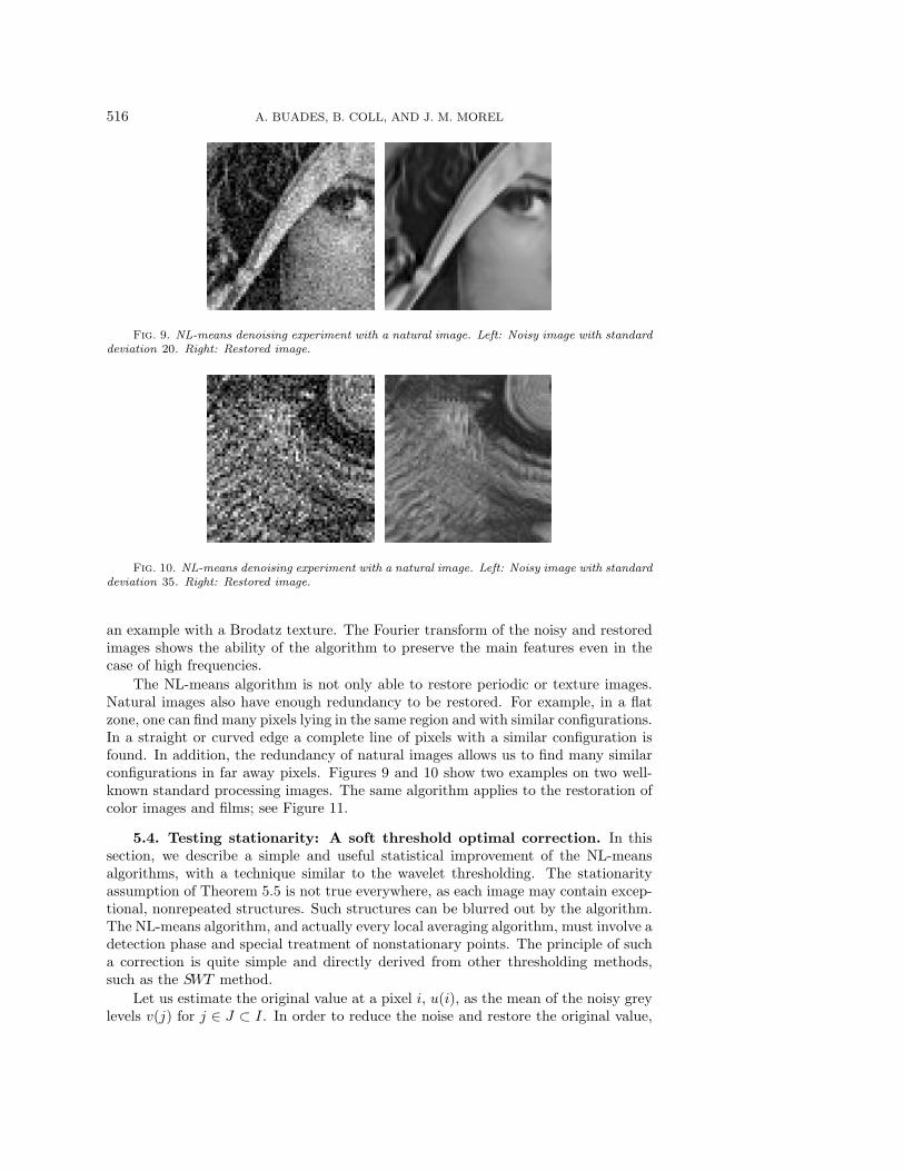
Fig. 9. NL-means denoising experiment with a natural image. Left: Noisy image with standarddeviation 20. Right: Restored image.

Fig. 10. NL-means denoising experiment with a natural image. Left: Noisy image with standarddeviation 35. Right: Restored image.

an example with a Brodatz texture. The Fourier transform of the noisy and restoredimages shows the ability of the algorithm to preserve the main features even in thecase of high frequencies.

The NL-means algorithm is not only able to restore periodic or texture images.Natural images also have enough redundancy to be restored. For example, in a flatzone, one can find many pixels lying in the same region and with similar configurations.In a straight or curved edge a complete line of pixels with a similar configuration isfound. In addition, the redundancy of natural images allows us to find many similarconfigurations in far away pixels. Figures 9 and 10 show two examples on two well-known standard processing images. The same algorithm applies to the restoration ofcolor images and films; see Figure 11.

5.4. Testing stationarity: A soft threshold optimal correction. In thissection, we describe a simple and useful statistical improvement of the NL-meansalgorithms, with a technique similar to the wavelet thresholding. The stationarityassumption of Theorem 5.5 is not true everywhere, as each image may contain excep-tional, nonrepeated structures. Such structures can be blurred out by the algorithm.The NL-means algorithm, and actually every local averaging algorithm, must involve adetection phase and special treatment of nonstationary points. The principle of sucha correction is quite simple and directly derived from other thresholding methods,such as the SWT method.

Let us estimate the original value at a pixel i, u(i), as the mean of the noisy greylevels v(j) for j ∈ J ⊂ I. In order to reduce the noise and restore the original value,


Fig. 11. NL-means denoising experiment with a color image. Left: Noisy image with standarddeviation 15 in every color component. Right: Restored image.

pixels j ∈ J should have a nonnoisy grey level u(j) similar to u(i). Assuming thisfact,

u(i) =1

|J |∑j∈J

v(j) � 1

|J |∑j∈J

u(i) + n(j) → u(i) as |J | → ∞,

because the average of noise values tends to zero. In addition,

1

|J |∑j∈J

(v(j) − u(i))2 � 1

|J |∑j∈J

n(j)2 → σ2 as |J | → ∞.

If the averaged pixels have a nonnoisy grey-level value close to u(i), as expected, thenthe variance of the average should be close to σ2. If it is a posteriori observed that thisvariance is much larger than σ2, this fact can hardly be caused only by the noise. Thismeans that the original grey-level values of the averaged pixels were very different.At those pixels, a more conservative estimate is required, and therefore the estimatedvalue should be averaged with the noisy one. The next result tells us how to computethis average.

Theorem 5.7. Let X and Y be two real random variables. Then the linearestimate Y ,

Y = EY +Cov(X,Y )

V arX(X − EY ),

minimizes the square error

mina,b∈R

E[(Y − (a + bX))2].

In our case, X = Y + N , where N is independent of Y , with zero mean andvariance σ2. Thus,

Y = EY +V arY

V arY + σ2(X − EY ),

which is equal to

Y = EX + max

(0,

V arX − σ2

V arX

)(X − EX).


Fig. 12. Optimal correction experience. Left: Noisy image. Middle: NL-means solution.Right: NL-means corrected solution. The average with the noisy image makes the solution noisier,but details and fine structure are better preserved.

This strategy can be applied to correct any local smoothing filter. However, a goodestimate of the mean and the variance at every pixel is needed. That is not the casefor the local smoothing filters of section 2. This strategy can instead be satisfactorilyapplied to the NL-means algorithm. As we have shown in the previous section, theNL-means algorithm converges to the conditional mean. The conditional variance canalso be computed by the NL-means algorithm, by taking φ(x) = x2 in Theorem 5.5,and then computing the variance as EX2 − (EX)2. In Figure 12 one can see anapplication of this correction.

5.5. Fast multiscale versions.

5.5.1. Plain multiscale. Let us now make some comments on the complexityof NL-means and how to accelerate it. One can estimate the complexity of an unso-phisticated version as follows. If we take a similarity window of size (2f + 1)2, andsince we can restrict the search of similar windows in a larger “search window” of size(2s+1)2, the overall complexity of the algorithm is N2 × (2f +1)2 × (2s+1)2, whereN2 is the number of pixels of the image. As for practical numbers, we took in allexperiments f = 3, s = 10, so that the final complexity is about 49× 441×N2. For a512× 512 image, this takes about 30 seconds on a normal PC. It is quite desirable toexpand the size of the search window as much as possible, and it is therefore usefulto give a fast version. This is easily done by a multiscale strategy, with little loss inaccuracy.

Multiscale algorithm.

1. Zoom out the image u0 by a factor 2 by a standard Shannon subsamplingprocedure. This yields a new image u1. For convenience, we denote by (i, j)the pixels of u1 and by (2i, 2j) the even pixels of the original image u0.

2. Apply NL-means to u1, so that with each pixel (i, j) of u1, a list of windowscentered in (i1, j1), . . . , (ik, jk) is associated.

3. For each pixel of u0, (2i+ r, 2j+s) with r, s ∈ {0, 1}, we apply the NL-meansalgorithm. But instead of comparing with all the windows in a searching zone,we compare only with the nine neighboring windows of each pixel (2il, 2jl)for l = 1, . . . , k.

4. This procedure can be applied in a pyramid fashion by subsampling u1 into u2,and so on. In fact, it is not advisable to zoom down more than twice.

By zooming down by just a factor 2, the computation time is divided by approxi-mately 16.

5.5.2. By blocks. Let I be the 2D grid of pixels, and let {i1, . . . , in} be a subsetof I. For each ik, let Wk ⊂ I be a neighborhood centered in ik, Wk = ik +Bk, whereBk gives the size and shape of the neighborhood. Let us suppose that each Wk is a


connected subset of I, such that I = W1 ∪ W2 ∪ · · · ∪ Wn, and where we allow theintersections between the neighborhoods to be nonempty.

Then for each Wk we define the vectorial NL-means as

NL(Wk) =1

Ck

∑j∈I

v(j + Bk)e− ‖v(ik+Bk)−v(j+Bk)‖2

2h2 ,

where Ck =∑

j∈I e− ‖v(ik+Bk)−v(j+Bk)‖2

2h2 and h acts as a filtering parameter. We note

that NL(Wk) is a vector of the same size as Wk. In contrast with the NL-meansalgorithm, we compute a nonweighted L2 distance, since we restore at the same timea whole neighborhood and do not want to give privilege to any point of the neighbor-hood.

In order to restore the value at a pixel i, we take into account all Wk containingi, Ai = {k | i ∈ Wk}, and define

NL(i) =1

|Ai|∑k∈Ai

NL(Wk)(i).

The overlapping of these neighborhoods permits a regular transition in the restoredimage and avoids block effects.

This variant by blocks of NL-means allows a better adaptation to the local imageconfiguration of the image and, at the same time, a reduction of the complexity. Inorder to illustrate this reduction, let us describe the simplest implementation:

• Let N × N be the size of the image, and set ik = (kn, kn) for k = 1, . . . ,(N − n)/n.

• Consider the subset B = {i = (xi, yi) | |xi| ≤ m and |yi| ≤ m} and Wk =ik + B for all k. We take m > n/2 in order to have a nonempty intersectionbetween neighboring subsets Wk.

• If we take a squared neighborhood B of size (2m+1)2, and since we can restrictthe search of similar windows in a larger “search window” of size (2s + 1)2,the overall complexity of the algorithm is (2m + 1)2 × (2s + 1)2 × (N−n

n )2.Taking n = 9 reduces the computation time of the original algorithm by more

than 81.

6. Discussion and comparison.

6.1. NL-means as an extension of previous methods. As was said before,the Gaussian convolution preserves only flat zones, while contours and fine structureare removed or blurred. Anisotropic filters instead preserve straight edges, but flatzones present many artifacts. One could think of combining these two methods toimprove both results. A Gaussian convolution could be applied in flat zones, while ananisotropic filter could be applied on straight edges. Still, other types of filters shouldbe designed to specifically restore corners or curved edges and texture. The NL-meansalgorithm seems to provide a feasible and rational method to automatically take thebest of each mentioned algorithm, reducing for every possible geometric configurationthe image method noise. Although we have not computed explicitly the image methodnoise, Figure 13 illustrates how the NL-means algorithm chooses in each case a weightconfiguration corresponding to one of the previously analyzed filters. In particular,according to this set of experiments, we can consider that the consistency results givenin Theorems 2.1, 2.3, and 2.5 are all valid for this algorithm.


(a) (b)

(c) (d)

(e) (f)

Fig. 13. On the right-hand side of each pair, we display the weight distribution used to estimatethe central pixel of the left image by the NL-means algorithm. (a) In flat zones, the weights aredistributed as a convolution filter (as a Gaussian convolution). (b) In straight edges, the weights aredistributed in the direction of the level line (as the mean curvature motion). (c) On curved edges,the weights favor pixels belonging to the same contour or level line, which is a strong improvementwith respect to the mean curvature motion. (d) In a flat neighborhood, the weights are distributed ina grey-level neighborhood (as with a neighborhood filter). In the cases of (e) and (f), the weights aredistributed across the more similar configurations, even though they are far away from the observedpixel. This shows a behavior similar to a nonlocal neighborhood filter or to an ideal Wiener filter.

In Figure 14 we display the probability distributions used to restore a noisy pixel.The images are the same of Figure 13. The comparison of both figures illustrates howthe probability distribution is perturbed by the addition of a white noise. In this case,the probability distribution is still adapted to the local configuration of the image,and the main structures of Figure 13 are well preserved.

6.2. Comparison. In this section we shall compare the different algorithmsbased on three well-defined criteria: the method noise, the mean square error, and thevisual quality of the restored images. Note that every criterion measures a differentaspect of the denoising method. It is easy to show that only one criterion is notenough to judge the restored image, and so one expects a good solution to have ahigh performance under the three criteria.


(a) (b)

(c) (d)

(e) (f)

Fig. 14. On the right-hand side of each pair, we display the weight distribution used to estimatethe central pixel of the left image by the NL-means algorithm. Images are obtained by adding aGaussian noise of standard deviation 12.5 to those of Figure 13.

6.2.1. Method noise comparison. In previous sections we have defined themethod noise and computed it for the different algorithms. Remember that the denois-ing algorithm is applied on the original (slightly noisy) image. A filtering parameter,depending mainly on the standard deviation of the noise, must be fixed for most al-gorithms. Let us fix σ = 2.5: we can suppose that any digital image is affected bythis amount of noise since it is not visually noticeable.

The method noise tells us which geometrical features or details are preserved bythe denoising process and which are eliminated. In order to preserve as many featuresas possible of the original image, the method noise should look as much as possiblelike white noise. Figures 15–17 display the method noise of the different methods fora set of standard natural images. Let us comment on them briefly.

• The Gaussian filter method noise highlights all important features of theimage, such as texture, contours, and details. All these features have a largeLaplacian and are therefore modified by the application of the algorithm; seeTheorem 2.1.

• As announced in Theorem 2.3, the anisotropic filter method noise displays


Fig. 15. Image method noise. From left to right and from top to bottom: original image,Gaussian convolution, mean curvature motion, total variation, Tadmor–Nezzar–Vese iterated totalvariation, Osher et al. total variation, neighborhood filter, soft TIWT, hard TIWT, DCT empiricalWiener filter, and the NL-means algorithm.

the corners and high frequency features. The straight edges are instead notto be seen: they have a low curvature.

• The total variation method modifies most structures and details of the image.Even straight edges are not well preserved.

• The iterated total variation refinements improve the total variation methodnoise. Both strategies try to reduce the geometry present in the removednoise, adding it back to the restored image, and therefore reducing the methodnoise.


Fig. 16. Image method noise. From left to right and from top to bottom: original image,total variation, neighborhood filter, hard TIWT, DCT empirical Wiener filter, and the NL-meansalgorithm.

Fig. 17. Image method noise. From left to right and from top to bottom: original image,total variation, neighborhood filter, hard TIWT, DCT empirical Wiener filter, and the NL-meansalgorithm.

• The neighborhood filter preserves flat objects and contrasted edges, whileedges with a low contrast are not kept. In any case, the contours, texture,and details seem to be well preserved.


• The TIHWT method noise is concentrated on the edges and high frequencyfeatures. These structures lead to coefficients of large enough value but lowerthan the threshold. They are removed by the algorithm. The average of theapplication to all translated versions reduces the method noise, and structuresare hardly noticeable.

• The TISWT method noise presents much more structure than the hard thresh-olding. Indeed, the method noise is not only based on the small coefficientsbut also on an attenuation of the large ones, leading to a high alteration ofthe original image.

• It is difficult to find noticeable structure in the DCT empirical Wiener filtermethod noise. Only some contours are noticeable. In general, this filter seemsto perform much better than all local smoothing filters and other frequencydomain filters. Its results are similar to those of a hard stationary waveletthresholding.

• The NL-means method noise looks more like a white noise.

6.2.2. Visual quality comparison. As commented on before, the visual qual-ity of the restored image is another important criterion to judge the performance ofa denoising algorithm. Let us present some experiments on a set of standard naturalimages. The objective is to compare the visual quality of the restored images, thenonpresence of artifacts, and the correct reconstruction of edges, texture, and finestructure. Figures 18–21 present these experiences comparing the visual quality ofprevious methods.

Figure 18 illustrates the fact that a nonlocal algorithm is needed for the correctreconstruction of periodic images. Local smoothing filters and local frequency filtersare not able to reconstruct the wall pattern. Only the NL-means algorithm and theglobal Fourier–Wiener filter reconstruct the original texture. The Fourier–Wienerfilter is based on a global Fourier transform which is able to capture the periodicstructure of the image in a few coefficients. Now, in practice, this is an ideal filterbecause the Fourier transform of the original image is used. Figure 13(e) showshow the NL-means method chooses the correct weight configuration and explains thecorrect reconstruction of the wall pattern.

Fig. 18. Denoising experience on a periodic image. From left to right and from top to bottom:noisy image (standard deviation 35), Gauss filtering, total variation, neighborhood filter, Wienerfilter (ideal filter), hard TIWT, DCT empirical Wiener filtering, and the NL-means algorithm.


Fig. 19. Denoising experience on a natural image. From left to right and from top to bottom:noisy image (standard deviation 35), neighborhood filter, total variation, Tadmor–Nezzar–Vese it-erated total variation, Osher et al. iterated total variation, and the NL-means algorithm.

Fig. 20. Denoising experience on a natural image. From left to right and from top to bot-tom: noisy image (standard deviation 35), neighborhood filter, total variation, and the NL-meansalgorithm.

Figures 19 and 20 illustrate the difficulty of local smoothing filters for recoveringstochastic patterns. The high degree of noise present in the image makes the localcomparisons of the neighborhood filter noise-dependent. As a consequence, noise andtexture are not well differentiated. The regularity assumption involved in the boundedvariation makes it unsuitable for the restoration of textures which are filtered asnoise. Iterated total variation refinements improve the total variation minimizationand recover part of the excessively filtered texture.

Figure 21 shows that the frequency domain filters are well adapted to the recoveryof oscillatory patterns. Although some artifacts are noticeable in both solutions, thestripes are well reconstructed. The DCT transform seems to be more adapted to thistype of texture, and stripes are a little better reconstructed. For a much more detailedcomparison between sliding window transform domain filtering methods and waveletthreshold methods, we refer the reader to [39]. Figure 22 shows that although thetotal variation minimization is not adapted to the restoration of oscillatory patterns,the iterated total variation approaches improve the restored image and reduce thisdrawback. The NL-means algorithm also performs well on this type of texture, due


Fig. 21. Denoising experience on a natural image. From left to right and from top to bottom:noisy image (standard deviation 25), the DCT empirical Wiener filter, hard TIWT, and the NL-means algorithm.

Fig. 22. Denoising experience on a natural image. From left to right and from top to bottom:noisy image (standard deviation 25), the total variation minimization, the Tadmor–Nezzar–Veseiterated total variation, and the Osher et al. iterated total variation.

to its high degree of redundancy.

Finally, in Figures 23 and 24 we show a real denoising experiment. The NL-meansalgorithm is applied to a natural image taken in poor light conditions. The NL-meansalgorithm seems to denoise the image, keeping the main structures and details.

6.2.3. Mean square error comparison. The mean square error is the squareof the Euclidean distance between the original image and its estimate. This numericalquality measurement is the more objective one, since it does not rely on any visual in-terpretation. Table 1 shows the mean square error of the different denoising methodswith the images presented in this paper. This error table seems to corroborate theobservations made for the other criteria. One sees, for example, how the frequency do-main filters have a lower mean square error than the local smoothing filters. One alsosees that in the presence of periodic or textural structures the empirical Wiener filterbased on a DCT transform performs better than the wavelet thresholding; see alsoFigures 18 and 21. Note that, in the presence of periodic or stochastic patterns, theNL-means mean square error is significantly more precise than the other algorithms.Of course, the errors presented in this table cannot be computed in a real denoisingproblem. Let us remark that a small error does not guarantee a good visual quality ofthe restored image. The mean square error by itself would not be meaningful, and allprevious quality criteria are also necessary to evaluate the performance of denoisingmethods.

Appendix. The set H of assumptions necessary for the statement of Theorem 5.5are the following:

(H1) The sequence of random vectors Zi = {Yi, Xi}∞i=1, where Yi is real valued andXi is R

p valued, form a strictly stationary sequence.


Fig. 23. Denoising experience on a natural noisy image. Top: Original image, Deia village(Mallorca). Bottom: NL-means filtered image.

(H2) The sequence {Zi} is β-mixing, and the sequence β(n) satisfies the followingsummability requirement: β∗ =

∑∞j=1 β(n) < ∞.

(H3) Let α = α(n) be a positive integer, and let μ = μ(n) be the largest positiveinteger for which 2αμ ≤ n. Then

lim sup[1 + 6e12β1/(μ+1)(α)]μ < ∞.

(H4) ‖x‖pK(x) → 0, as x → ∞, where the norm ‖x‖ of x = (x1, . . . , xp) is definedby ‖x‖ = max(|x1|, . . . , |xp|).


Fig. 24. Detail of Figure 23. Top: Original detail. Bottom: NL-means filtered detail.

Table 1

Mean square error table. A smaller mean square error indicates that the estimate is closer tothe original image. The numbers have to be compared on each row. The square of the number onthe left-hand column gives the real variance of the noise. By comparing this square to the values onthe same row, it is quickly checked that all studied algorithms indeed perform some denoising. Thisis a sanity check! In general, the comparison performance corroborates the previously mentionedquality criteria.

Image σ GF AF TV YNF EWF TIHWT NL-means

Boat 8 53 38 39 39 33 28 23Lena 20 120 114 110 129 105 81 68Barbara 25 220 216 186 176 111 135 72Baboon 35 507 418 365 381 396 365 292Wall 35 580 660 721 598 325 712 59

(H5) (i) φ is a real valued Borel function defined on R such that E|φ(Y )|s < ∞for some s > 1.

(ii)

sup

[∫R

|φ(y)|sfXY (x, y)dy; x ∈ Rp

]= C < ∞.

(H6) (i) For any point x and x′ in Rp and for some positive constant C (inde-

pendent of these points),

|K(x) −K(x′)| ≤ C‖x− x′‖.

(ii)∫‖x‖K(x)dx < ∞.

(H7) For any point x in Rp, there are positive constants C(x) such that, for all

x′ ∈ Rp and with J being as in (H8),

(i)

‖fX(x) − fX(x′)‖ ≤ C(x)‖x− x′‖, sup[C(x); x ∈ J ] < ∞.

(ii)

‖ψ(x) − ψ(x′)‖ ≤ C(x)‖x− x′‖, sup[C(x); x ∈ J ] < ∞,

where r(x) = E[φ(Y ) | X = x] and ψ(x) = r(x)fX(x).


(H8) There exists a compact subset J of Rp such that

inf[fX(x); x ∈ J ] > 0.

Acknowledgments. We thank Francois Malgouyres, Stephane Mallat, YvesMeyer, Stanley Osher, Guillermo Sapiro, and Luminita Vese for valuable conversa-tions and comments. Several experiments in this paper have been performed thanksto the public software libraries MegaWave, Wavelab, and Advanced Image ProcessingLab.

REFERENCES

[1] L. Alvarez, P.-L. Lions, and J.-M. Morel, Image selective smoothing and edge detection bynonlinear diffusion. II, SIAM J. Numer. Anal., 29 (1992), pp. 845–866.

[2] J.-F. Aujol, G. Aubert, L. Blanc-Feraud, and A. Chambolle, Image decomposition intoa bounded variation component and an oscillating component, J. Math. Imaging Vision,22 (2005), pp. 71–88.

[3] S. A. Awate and R. T. Whitaker, Image denoising with unsupervised, information-theo-retic, adaptive filtering, in Proceedings of the IEEE International Conference on ComputerVision and Pattern Recognition, 2005, to appear.

[4] A. Buades, B. Coll, and J.-M. Morel, Procede de traitement de donnees d’image, parreduction de bruit d’image, et camera integrant des moyens de mise en oeuvre du procede(Image data process by image noise reduction and camera integrating the means for im-plementing this process), French patent application, serial number: 0404837.

[5] F. Catte, F. Dibos, and G. Koepfler, A morphological scheme for mean curvature motionand applications to anisotropic diffusion and motion of level sets, SIAM J. Numer. Anal.,32 (1995), pp. 1875–1909.

[6] A. Chambolle and P. L. Lions, Image recovery via total variation minimization and relatedproblems, Numer. Math., 76 (1997), pp. 167–188.

[7] T. F. Chan and H. M. Zhou, Total variation improved wavelet thresholding in image com-pression, in Proceedings of the IEEE International Conference on Image Processing, Vol. 2,Vancouver, BC, Canada, 2000, pp. 391–394.

[8] R. R. Coifman and D. Donoho, Translation-invariant de-noising, in Wavelets and Statistics,Springer-Verlag, New York, 1995, pp. 125–150.

[9] D. Donoho, De-noising by soft-thresholding, IEEE Trans. Inform. Theory, 41 (1995), pp. 613–627.

[10] D. Donoho and I. Johnstone, Ideal spatial adaptation via wavelet shrinkage, Biometrika, 81(1994), pp. 425–455.

[11] S. Durand and M. Nikolova, Restoration of wavelet coefficients by minimizing a speciallydesigned objective function, in Proceedings of the IEEE Workshop on Variational and LevelSet Methods in Computer Vision, 2003.

[12] S. Durand and J. Froment, Reconstruction of wavelet coefficients using total variation min-imization, SIAM J. Sci. Comput., 24 (2003), pp. 1754–1767.

[13] A. Efros and T. Leung, Texture synthesis by non parametric sampling, in Proceedings ofthe IEEE International Conference on Computer Vision, Vol. 2, Corfu, Greece, 1999, pp.1033–1038.

[14] F. Guichard, J. M. Morel, and R. Ryan, Image Analysis and P.D.E.’s, preprint.[15] E. Le Pennec and S. Mallat, Geometrical image compression with bandelets, in Proceedings

of the SPIE 2003, Vol. 5150, Lugano, Switzerland, 2003, pp. 1273–1286.[16] E. Levina, Statistical Issues in Texture Analysis, Ph.D. thesis, UC-Berkeley, Berkeley, CA,

2002.[17] M. Lindenbaum, M. Fischer, and A. M. Bruckstein, On Gabor contribution to image en-

hancement, Pattern Recognition, 27 (1994), pp. 1–8.[18] S. Lintner and F. Malgouyres, Solving a variational image restoration model which involves

L∞ constraints, Inverse Problems, 20 (2004), pp. 815–831.[19] F. Malgouyres, A noise selection approach of image restoration, in Proceedings of Wavelet

Applications in Signal and Image Processing IX, SPIE Proc. Ser. 4478, SPIE, Bellingham,WA, 2001, pp. 34–41.

[20] S. Mallat, A Wavelet Tour of Signal Processing, Academic Press, San Diego, CA, 1997.[21] B. Merriman, J. Bence, and S. Osher, Diffusion generated motion by mean curvature, in

Proceedings of the Geometry Center Workshop, Minneapolis, MN, 1992.


[22] Y. Meyer, Oscillating Patterns in Image Processing and Nonlinear Evolution Equations, Univ.Lecture Ser. 22, AMS, Providence, RI, 2002.

[23] E. A. Nadaraya, On non-parametric estimates of density functions and regression curves,Theory Probab. Appl., 10 (1964), pp. 186–190.

[24] E. Ordentlich, G. Seroussi, S. Verdu, M. Weinberger, and T. Weissman, A discreteuniversal denoiser and its application to binary images, in Proceedings of the IEEE Inter-national Conference on Image Processing, Vol. 1, Barcelona, Spain, 2003, pp. 117–120.

[25] S. Osher, M. Burger, D. Goldfarb, J. Xu, and W. Yin, An iterative regularization methodfor total variation-based image restoration, Multiscale Model. Simul., 4 (2005), pp. 460–489.

[26] S. Osher, A. Sole, and L. Vese, Image decomposition and restoration using total variationminimization and the H−1 norm, Multiscale Model. Simul., 1 (2003), pp. 349–370.

[27] P. Perona and J. Malik, Scale space and edge detection using anisotropic diffusion, IEEETrans. Patt. Anal. Mach. Intell., 12 (1990), pp. 629–639.

[28] G. G. Roussas, Nonparametric regression estimation under mixing conditions, Stochastic Pro-cess. Appl., 36 (1990), pp. 107–116.

[29] L. Rudin and S. Osher, Total variation based image restoration with free local constraints,in Proceedings of the IEEE International Conference on Image Processing, Vol. 1, Austin,TX, 1994, pp. 31–35.

[30] L. Rudin, S. Osher, and E. Fatemi, Nonlinear total variation based noise removal algorithms,Phys. D, 60 (1992), pp. 259–268.

[31] C. Shannon and W. Weaver, The Mathematical Theory of Communication, University ofIllinois Press, Champaign, IL, 1998.

[32] A. Sharf, M. Alexa, and D. Cohen-Or, Context-based surface completion, in Proceedings ofthe 31st International Conference on Computer Graphics and Interactive Techniques, LosAngeles, CA, 2004, pp. 878–887.

[33] S. M. Smith and J. M. Brady, SUSAN - a new approach to low level image processing,International Journal of Computer Vision, 23 (1997), pp. 45–78.

[34] J. Starck, E. Candes, and D. Donoho, The curvelet transform for image denoising, IEEETrans. Image Process., 11 (2000), pp. 670–684.

[35] E. Tadmor, S. Nezzar, and L. Vese, A multiscale image representation using hierarchical(BV,L2) decompositions, Multiscale Model. Simul., 2 (2004), pp. 554–579.

[36] L. Vese and S. Osher, Modeling textures with total variation minimization and oscillatingpatterns in image processing, J. Sci. Comput., 19 (2003), pp. 553–572.

[37] G. S. Watson, Smooth regression analysis, Sankhya Ser. A, 26 (1964), pp. 359–372.[38] T. Weissman, E. Ordentlich, G. Seroussi, S. Verdu, and M. Weinberger, Universal

discrete denoising: Known channel, IEEE Trans. Inform. Theory, 51 (2005), pp. 5–28.[39] L. Yaroslavsky, K. Egiazarian, and J. Astola, Transform domain image restoration meth-

ods: Review, comparison and interpretation, in Nonlinear Image Processing and PatternAnalysis, SPIE, Bellingham, WA, 2001, pp. 155–169.

[40] L. P. Yaroslavsky, Digital Picture Processing. An Introduction, Springer-Verlag, Berlin, 1985.[41] L. Yaroslavsky and M. Eden, Fundamentals of Digital Optics, Birkhauser Boston, Boston,

MA, 1996.[42] L. Yaroslavsky, Local adaptive image restoration and enhancement with the use of DFT and

DCT in a running window, in Proceedings of Wavelet Applications in Signal and ImageProcessing IV, SPIE Proc. Ser. 2825, Denver, CO, 1996, pp. 1–13.

pdfs.semanticscholar.orgpdfs.semanticscholar.org/e36c/cf21710de71a6deee44... · multiscale model....

Documents