Applications of the Seiberg-Witten

equations to the Differential Geometry

of non-compact Kahler manifolds

A Dissertation Presented

by

Ilya Elson

to

The Graduate School

in Partial Fulfillment of the Requirements

for the Degree of

Doctor of Philosophy

in

Mathematics

Stony Brook University

August 2014

Stony Brook University

The Graduate School

Ilya Elson

We, the dissertation committee for the above candidate for the Doctor ofPhilosophy degree, hereby recommend acceptance of this dissertation.

Claude LeBrun – Dissertation AdvisorProfessor, Department of Mathematics

H. Blaine Lawson, Jr. – Chairperson of DefenseDistinguished Professor, Department of Mathematics

Michael AndersonProfessor, Department of Mathematics

Martin RocekProfessor, Department of Physics

Stony Brook University

This dissertation is accepted by the Graduate School.

Charles TaberDean of the Graduate School

ii

Abstract of the Dissertation

Applications of the Seiberg-Witten equationsto the Differential Geometry of non-compact

Kahler manifolds

by

Ilya Elson

Doctor of Philosophy

in

Mathematics

Stony Brook University

2014

Soon after the introduction of the Seiberg-Witten equations, and

their magnificent application to the differential topology of 4-

manifolds, LeBrun [LeB95a] used these equations to study dif-

ferential geometry and prove a rigidity theorem for compact com-

plex hyperbolic manifolds. Biquard [Biq97] extended these re-

sults to non-compact, finite volume complex hyperbolic manifolds,

and Rollin [Rol04] extended these techniques to CH2. Finally,

Di Cerbo[DC12, DC11] applied Biquard’s techniques to Σ× Σg.

The main tool that allows one to use the Seiberg-Witten equations to

iii

study differential geometry is an integral scalar curvature estimate.

The principle difficulty in extending these methods to the non-

compact case, which was overcome by Biquard, Rollin and Di Cerbo

is the proof of the existence of a solution to the equations. Finally,

in LeBrun used conformal rescaling of the Seiberg-Witten equations

to prove an integral estimate that involves both the scalar and Weyl

curvature.

In this thesis we extend these techniques to quasiprojective 4-

manifolds which admit negatively curved, finite volume Kahler-

Einstein metrics. Following Biquard’s method we produce an

irreducible solution to the Seiberg-Witten equations on the non-

compact manifold as a limit of solutions on the compactification,

and then use the Weitzenbock formula to obtain a scalar curvature

estimate that is necessary for geometric applications.

iv

Dedicated to my grandfather, Yuri Lyubich.

v

Contents

Acknowledgements viii

1 Introduction 1

1.1 Summary of results . . . . . . . . . . . . . . . . . . . . . . . . 2

1.2 Preliminaries . . . . . . . . . . . . . . . . . . . . . . . . . . . 3

1.2.1 Spin and SpinC structures . . . . . . . . . . . . . . . . 3

1.2.2 Clifford bundles and the Dirac operator . . . . . . . . . 13

1.2.3 Weitzenbock Formulas . . . . . . . . . . . . . . . . . . 13

1.2.4 Differential Geometry in dimension 4 . . . . . . . . . . 16

1.3 Seiberg-Witten equations . . . . . . . . . . . . . . . . . . . . . . 17

1.3.1 The equations and basic properties . . . . . . . . . . . 18

1.3.2 The Seiberg-Witten equations on Kahler manifolds . . 28

2 Quasiprojective manifolds 29

2.1 Cheng-Yau Holder Spaces . . . . . . . . . . . . . . . . . . . . 29

2.2 Approximating metrics . . . . . . . . . . . . . . . . . . . . . . 30

2.3 Existence . . . . . . . . . . . . . . . . . . . . . . . . . . . . . 36

vi

2.4 Alternate Approach to Existence of Solutions of the Seiberg-

Witten equtions . . . . . . . . . . . . . . . . . . . . . . . . . . 40

2.5 Geometric Consequences . . . . . . . . . . . . . . . . . . . . . 50

2.5.1 L2-cohomology . . . . . . . . . . . . . . . . . . . . . . 50

2.5.2 Scalar curvature estimate . . . . . . . . . . . . . . . . 53

2.5.3 Gauss-Bonnet and Hirzebruch . . . . . . . . . . . . . . 55

2.5.4 Einstein metrics on blow-ups . . . . . . . . . . . . . . . 56

3 Weyl Curvature Estimates 58

3.1 Compact Case . . . . . . . . . . . . . . . . . . . . . . . . . . . 58

3.2 Non-compact Case . . . . . . . . . . . . . . . . . . . . . . . . 60

3.3 Non-existence of Einstein metrics on blow-ups . . . . . . . . . 64

A Analysis 65

Bibliography 73

vii

Acknowledgements

First and foremost I would like to thank my advisor Prof. Claude LeBrun

for his guidance, for kindly sharing his time with me, for his patience and

encouragement.

I would like to thank my parents, Yuri and Genie Elson, for all their support

during my years in graduate school. I would like to thank Misha Lyubich for

many mathematical discussions, which were very useful for me. I would like to

thank my grandfather, Yuri Lyubich, for teaching me most of the mathematics

I know.

I would also like to thank my friends both at Stony Brook and at MIT for

their friendship and support. Espeically, I would like to thank Max Lipyanskiy

for our many interesting discussions. Finally, I would like to thank Deepika

Vasudevan, without whom, I would not have completed this thesis.

viii

Chapter 1

Introduction

The first appearance of gauge theory in physics was the theory of Electricity

and Magnetism developed by Maxwell in [Max65], though, without the modern

language of gauge theory or even modern vector calculus notation. The

second appearance of gauge theory is Einstein’s theory of general relativity

in [Ein16]. It was Weyl in [Wey29] who in his attempt to unify Electricity and

Magnetism with Einstein’s Theory of Gravitation, enunciated the principle

of gauge invariance or Eichinvarianz in German. The ascendance of gauge

theory as the foundation of modern physics dates to the paper of Yang and

Mills [YM54], which introduced non-abelian gauge theory. An account of the

history of gauge theory can be found in [JO01].

On the mathematical side, gauge theory is the study of connections, initiated

by Cartan in [Car23]. The development of the modern theory of connections

on fiber bundles was initiated by Ehresmann in [Ehr51]. Since then the study

of connections and their curvatures has led to a rich and beautiful theory. No

attempt will be made to summarize this theory or even its basic definitions,

1

for many such expositions exist in the literature, e. g. [Tay11b, DK90].

Instead, the first chapter consists of a concise exposition of the notions

necessary to write down the Seiberg-Witten equations (1.3.1) and prove the

basic theorems in Seiberg-Witten theory. This summary is aimed at a student

of differential geometry, who may be interested in applications of Seiberg-

Witten to differential geometry but who does not wish to delve into a detailed

exposition of Seiberg-Witten theory. Section 1.1 contains a summary of the

main results of the thesis, for the convenience of the reader.

1.1 Summary of results

The main results of this thesis are:

• Theorem 2.3.1, which shows existence of irreducible solutions to the

Seiberg-Witten equations on quasi-projective manifolds with metrics

C2-close to the Kahler-Einstein metric.

• Theorem 2.5.3, which is a scalar curvature estimate which can be derived

from the Weitzenbock formula.

• Theorem 2.5.6, which asserts the non-existence of Einstein metrics on

k-fold blow-ups of quasi-projective manifolds, which are asymptotic to

the Kahler-Einstein metric, with k > 23

(c1(KX) + c1(LD))2.

• Proposition 3.2.1, which is a mixed Weyl and scalar curvature estimate,

based on a conformal rescaling argument.

2

• Theorem 3.3.1, which improves the bound on k by a factor of 2 to

k > 13

(c1(KX) + c1(LD))2.

1.2 Preliminaries

1.2.1 Spin and SpinC structures

A classic and comprehensive reference for Sections 1.2.1 – 1.2.4 is [LM89]. A

much shorter and less comprehensive introduction, however, can be found in the

expositions of Seiberg-Witten theory in [Mor96], and a very concise exposition

can be found in [Tay11c, Chapter 10]. In the following, all manifolds will be

assumed smooth, and a closed manifold will mean a compact manifold without

boundary. Let M be a closed, orientable Riemannian manifold of dimension

n and let E be an orientable rank r vector bundle over M . The choice of a

bundle metric g on E reduces the structure group of E from GL(r) to O(r).

Now let us choose an orientation on E. This has the effect of further reducing

the structure group of E to SO(r). We have, thus, reduced the structure group

of E from a group with π0 = Z2 to one with π0 = 0. It is then natural to

ask whether we can further change the structure group to a simply connected

group. E is called spinnable if we can lift the structure group of E from SO(r)

to Spin(r), the double cover of SO(r), and a choice of such a lift is called a

spin structure on E, or just spin structure, in the case E = TM , the tangent

bundle of M .

To describe the above construction in greater detail, let us denote by PG(E)

the principal G-bundle associated to a vector bundle E with structure group G.

3

Definition 1.2.1. A spin structure on an orientable rank r vector bundle E,

is Spin(r)-principal bundle whose total space, PSpin(r) is a double cover of the

total space PSO(r)(E) of the principal SO(r)-bundle associated to E, which

restricts to the cover Spin(r)→ SO(r) on each fiber. This definition is neatly

summarized in the following commutative diagram:

Spin(r)π

> SO(r)

Z2

>

>PSpin(r)(E)

∨π

> PSO(r)(E)∨

M<

>

Figure 1.2.1

where π is a double cover which restricts to π on each fiber, so that for

p ∈ PSpin(r)(E) and g ∈ Spin(r), π(pg) = π(p)π(g). A spin structure on a

manifold is a spin structure on its tangent bundle.

Not every orientable vector bundle is spinnable. In fact, an orientable vector

bundle is spinnable if and only if w2(E), its second Stiefel-Whitney class is 0.

Indeed, essentially by definition we can regard a principal SO(r) bundle over

M as an element of the Cech cohomology group H1(M ; E(SO(r))), where E(G)

is the sheaf of functions on M with values in G. The short exact sequence of

4

coefficient groups

0 → Z2 → Spin(r)→ SO(r)→ 0

gives rise to a long exact sequence of Cech cohomology groups, though, the

long exact sequence terminates at the H2(M ;Z2) term since H2(M ; E(G)) is

not defined for non-abelian G,

0 → H1(M ;Z2)→ H1(M ; E(Spin(r)))→ H1(M ; E(SO(r)))δ−→ H2(M ;Z2)

The boundary map δ can be identified with w2 by computation on the universal

SO(r) bundle since the long exact sequence is natural. This shows that w2 is

the obstruction to a bundle being spinnable.

There is another important exact sequence relevant to the discussion of spin

structures that arises from the Serre spectral sequence of a fibration. See [Hat]

for an introduction to spectral sequences in general, and the Serre spectral

sequence in particular. Consider the E2 page of the Serre spectral sequence

for the fibration SO(r)ι−→ PSO(r)(E) → M with Z2 coefficients. We have

Ep,q2 = Hp(M ;Hq(SO(r);Z2)) and

1 H1(SO(r),Z2)

0 Z2 H1(M,Z2) H2(M,Z2)

0 1 2

where we have substituted H0(SO(r);Z2) = Z2.

In this portion of the spectral sequence there is only one non-trivial differ-

ential d0,12 : H1(M ;Z2)→ H2(M ;Z2). The Serre spectral sequence then tells

5

us that H1(PSO(r)(E);Z2) has a filtration with ker d0,12 and H1(M ;Z2) as the

successive quotients. In other words, there exists 0 ⊂ F ⊂ H1(PSO(r)(E);Z2)

such that F/0 ∼= H1(M ;Z2) and H1(PSO(r)(E);Z2)/F ∼= ker d0,12 . Note that

while the filtration is natural, the isomorphisms above are not. Hence, we get

two natural sequences, the first is exact, and the second is exact at the first

and second terms:

H1(M ;Z2) → H1(PSO(r)(E);Z2) ker d0,12 (1.2.1)

ker d0,12 → H1(SO(r);Z2)

d0,12−−→ H2(M ;Z2) (1.2.2)

which we can combine to get the long exact sequence

H1(M ;Z2) → H1(PSO(r)(E);Z2)→ H1(SO(r);Z2)︸ ︷︷ ︸Z2

d0,12−−→ H2(M ;Z2) (1.2.3)

Now given a topological space X, the double covers of X, which we denote

X, are in one-to-one correspondence with conjugacy classes of index 2 sub-

groups of π1(X, x0). Since an index 2 subgroup is automatically normal, double

covers of X are actually in one to one correspondence with homomorphisms

π1(X, x0)→ Z2. Further, since Z2 is abelian any homomorphism to Z2 auto-

matically contains the commutator subgroup of the domain in the kernel, and

since H1(X;Z) is isomorphic to π1(X, x0) modulo the commutator subgroup,

we see that double covers of X are actually in one to one correspondence with

homomorphisms from H1(X;Z)→ Z2. But Hom(H1(X;Z),Z2) ∼= H1(X;Z2)

by the universal coefficients theorem since Ext(Z,Z2) vanishes. Hence, Spin

structures, which are double covers of PSO(r)(E) which restrict to the dou-

6

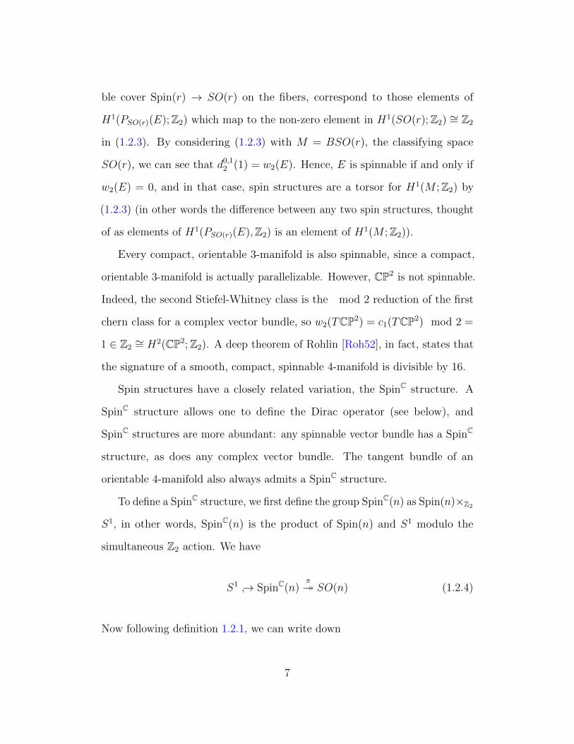
ble cover Spin(r) → SO(r) on the fibers, correspond to those elements of

H1(PSO(r)(E);Z2) which map to the non-zero element in H1(SO(r);Z2) ∼= Z2

in (1.2.3). By considering (1.2.3) with M = BSO(r), the classifying space

SO(r), we can see that d0,12 (1) = w2(E). Hence, E is spinnable if and only if

w2(E) = 0, and in that case, spin structures are a torsor for H1(M ;Z2) by

(1.2.3) (in other words the difference between any two spin structures, thought

of as elements of H1(PSO(r)(E),Z2) is an element of H1(M ;Z2)).

Every compact, orientable 3-manifold is also spinnable, since a compact,

orientable 3-manifold is actually parallelizable. However, CP2 is not spinnable.

Indeed, the second Stiefel-Whitney class is the mod 2 reduction of the first

chern class for a complex vector bundle, so w2(TCP2) = c1(TCP2) mod 2 =

1 ∈ Z2∼= H2(CP2;Z2). A deep theorem of Rohlin [Roh52], in fact, states that

the signature of a smooth, compact, spinnable 4-manifold is divisible by 16.

Spin structures have a closely related variation, the SpinC structure. A

SpinC structure allows one to define the Dirac operator (see below), and

SpinC structures are more abundant: any spinnable vector bundle has a SpinC

structure, as does any complex vector bundle. The tangent bundle of an

orientable 4-manifold also always admits a SpinC structure.

To define a SpinC structure, we first define the group SpinC(n) as Spin(n)×Z2

S1, in other words, SpinC(n) is the product of Spin(n) and S1 modulo the

simultaneous Z2 action. We have

S1 → SpinC(n)π SO(n) (1.2.4)

Now following definition 1.2.1, we can write down

7

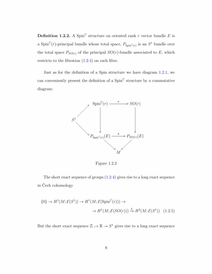
Definition 1.2.2. A SpinC structure on oriented rank r vector bundle E is

a SpinC(r)-principal bundle whose total space, PSpinC(r) is an S1 bundle over

the total space PSO(r) of the principal SO(r)-bundle associated to E, which

restricts to the fibration (1.2.4) on each fiber.

Just as for the definition of a Spin structure we have diagram 1.2.1, we

can conveniently present the definition of a SpinC structure by a commutative

diagram:

SpinC(r)π

> SO(r)

S1

>

>PSpinC(r)(E)

∨π

> PSO(r)(E)∨

M<

>

Figure 1.2.2

The short exact sequence of groups (1.2.4) gives rise to a long exact sequence

in Cech cohomology

0 → H1(M ; E(S1))→ H1(M ; E(SpinC(r)))→

→ H1(M ; E(SO(r)))δ−→ H2(M ; E(S1)) (1.2.5)

But the short exact sequence Z → R S1 gives rise to a long exact sequence

8

in cohomology

H1(M ; E(R))︸ ︷︷ ︸0

→ H1(M ; E(S1))c1−→ H2(M ;Z)→ H2(M ; E(R))︸ ︷︷ ︸

0

→

→ H2(M ; E(S1))W3−−→ H3(M ;Z)→ H3(M ; E(R))︸ ︷︷ ︸

0

(1.2.6)

Since Hk(M ; E(R)) = 0, (1.2.6) shows that H1(M ; E(S1)) is isomorphic

to H2(M ;Z) (the isomorphism is the first Chern class) and H2(M ; E(S1)) is

isomorphic to H3(M ;Z) (the isomorphism is the so-called “integer Stiefel-

Whitney class” W3). The W3 class is the image of w2, the ordinary second

Stiefel-Whitney class, under the Bockstein homomorphism in the cohomology

long exact sequence which arises from the short exact sequence Z ×2→ Z Z2:

· · · → H2(M ;Z)→ H2(M ;Z)→ H2(M ;Z2)β−→ H3(M ;Z)→ · · ·

W3 = β(w2). Now (1.2.5) becomes

0 → H2(M ;Z)→ H1(M ; E(SpinC(r)))→ H1(M ; E(SO(r)))W3−−→ H3(M ;Z)

(1.2.7)

It follows that a vector bundle has a SpinC structure if and only if its W3 class

vanishes. There is also a long exact sequence analogous to (1.2.3) that arises

from the Serre spectral sequence for the fibration SO(r) → PSO(r)(E) M

with Z coefficients. In this case, the E2 page of the spectral sequence is

9

2 H2(SO(r);Z) ∼= Z

1 H1(SO(r);Z) ∼= 0 0 0 0

0 Z H1(M ;Z) H2(M ;Z) H3(M ;Z)

0 1 2 3

There are no non-trivial differentials on the portion of the E2 page shown, so

this fragment survives to the E3 page, where the only non-trivial differential in

the portion of the spectral sequence that is shown is

d0,23 : H2(SO(r);Z)→ H3(M ;Z).

Just as in the discussion concerning Spin structures, there is a filtration of

H2(PSO(r)(E);Z) with successive quotients isomorphic to ker d0,23 and H2(M ;Z).

In other words, there exists 0 ⊂ F ⊂ H2(PSO(r)(E);Z) such that F/0 ∼=

H2(M ;Z) and H2(PSO(r)(E);Z)/F ∼= ker d0,23 . This gives us the long exact

sequence:

H2(M ;Z) → H2(PSO(r)(E);Z)→ H2(SO(r);Z)d0,23−−→ H3(M ;Z) (1.2.8)

By computation on the universal SO(r) bundle SO(r) → ESO(r)

BSO(r), we see that d0,23 (1) = W3(E). Now, BS1 ∼= CP∞, the classifying

space for complex line bundles, or equivalently for orientable rank 2 real vector

bundles, is also the Eilenberg-MacLane space K(Z, 2), hence homotopy classes

of maps X → CP∞, [X,CP∞] ∼= H2(X;Z). Or in other words, S1 bundles

on X are in one-to-one correspondence with elements of H2(X;Z). SpinC

10

structures are S1 bundles over PSO(r)(E) which restrict to

S1 → SpinC(r)→ SO(r),

as in 1.2.2. By (1.2.8) a SpinC structure exists if and only if W3(E) is 0, and in

that case the set of SpinC structures has a free transitive action of H2(M ;Z).

The SpinC story is very much analogous to the one for Spin structures.

Let us consider a few examples of Spin and SpinC structures.

Example 1.2.3. Let M = S1. There are two Spin structures on E = TS1,

the tangent bundle of S1. SO(1) = 1 and Spin(1) = Z2. One Spin structure

has PSpin(1)(TS1) = Z2 × S1 → PSO(1)(TS

1) = 1 × S1 with the map being

the only map Z2 → 1. The other Spin structure is given by the commutative

diagram 1.2.3 where π and the projection from PSpin(1)(TS1) to S1 are given

Spin(1) ∼= Z2π

> SO(1) ∼= 1

Z2

>

>PSpin(1)(TS

1) ∼= S1∨

π> PSO(r)(TS

1) ∼= S1∨

S1 <>

Figure 1.2.3

by z 7→ z2 (where S1 = z ∈ C | |z| = 1 ).

11

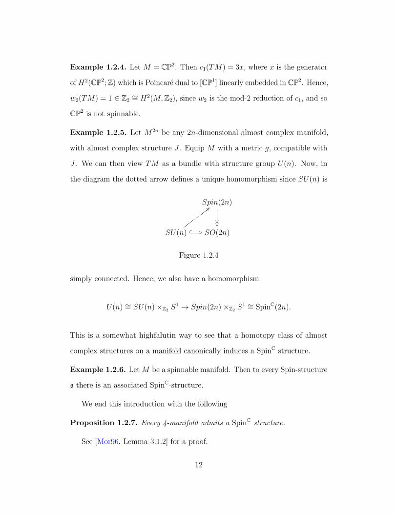
Example 1.2.4. Let M = CP2. Then c1(TM) = 3x, where x is the generator

of H2(CP2;Z) which is Poincare dual to [CP1] linearly embedded in CP2. Hence,

w2(TM) = 1 ∈ Z2∼= H2(M,Z2), since w2 is the mod-2 reduction of c1, and so

CP2 is not spinnable.

Example 1.2.5. Let M2n be any 2n-dimensional almost complex manifold,

with almost complex structure J . Equip M with a metric g, compatible with

J . We can then view TM as a bundle with structure group U(n). Now, in

the diagram the dotted arrow defines a unique homomorphism since SU(n) is

Spin(2n)

SU(n) ⊂ >.....

..........

......>

SO(2n)

∨∨

Figure 1.2.4

simply connected. Hence, we also have a homomorphism

U(n) ∼= SU(n)×Z2 S1 → Spin(2n)×Z2 S

1 ∼= SpinC(2n).

This is a somewhat highfalutin way to see that a homotopy class of almost

complex structures on a manifold canonically induces a SpinC structure.

Example 1.2.6. Let M be a spinnable manifold. Then to every Spin-structure

s there is an associated SpinC-structure.

We end this introduction with the following

Proposition 1.2.7. Every 4-manifold admits a SpinC structure.

See [Mor96, Lemma 3.1.2] for a proof.

12

1.2.2 Clifford bundles and the Dirac operator

Dirac introduced, what we now call, the Dirac operator in [Dir28], to explain

the splitting of the energy levels of the electron in the hydrogen atom, by

introducing a relativistic equation to replace the Schrodinger equation. The

latter cannot possibly be Lorentz invariant, since the Schrodinger equation is

first order in the time variable but second order in the spatial variables. This

led Dirac to search for a first order differential operator which squares to the

Laplacian.

Such an operator must have matrix coefficients and act on vector-valued

functions. For example, let σ1 = ( 0 11 0 ), σ2 = ( 0 −i

i 0 ) σ3 = ( 1 00 −1 ), be the Pauli

matrices, which satisfy σiσj + σjσi = 2δijI, where I is the identity matrix.

Then the operator D =∑3

i=1 σi∂i, acting on functions ψ : R3 → C2 satisfies

D2 = ∆. The operator that Dirac wrote down in [Dir28] is∑4

µ=1 γµ∂µ, where

γµ are 4 by 4 matrices, satisfying, γµγν + γνγµ = 2δµνI. This latter relation

is, of course, the Clifford relation, and is the starting point for the following

definitions and constructions leading to the generalization of the Dirac operator

to a differential operator acting on Clifford bundles.

1.2.3 Weitzenbock Formulas

Since the square of the Dirac operator, D∗D which we can call the Dirac

laplacian has the same principal symbol as the connection laplacian ∇∗∇ the

difference of the two is a differential operator of order at most one. Remarkably,

this difference is in fact a zeroth order operator, expressible in terms of the

curvature. Formulas that express the difference between two second order

13

differential operators that both have the same principal symbol as the laplacian

are usually called Weitzenbock Formulas. A concise exposition of this can

be found in [Tay11b, Section 10.4], [Roe98, Chapter 3], [Bou81a] or [LM89,

Chapter 2 §8]. Less classical but nevertheless helpful expositions can also be

found in [Pet, Lab07].

Indeed, let M be a Riemannian manifold, E →M be a Hermitian vector

bundle, with a metric connection, and also a Clifford module over TM , as

in the previous section. Let D be the Dirac operator on E, φ ∈ Γ(E), and

f ∈ C∞(M). We can directly compute

D∗D(fφ) = f D∗D φ− 2∇grad fφ− (∆f)φ.

But we can also compute ∇∗. Let α ∈ Ω1(M), then

∇∗f(α⊗ φ) = f∇∗(α⊗ φ)− 〈df, α〉φ

and if a vector field V ∈ Γ(TM) is defined by 〈V,W 〉 = α(W ), then

∇∗(α⊗ φ) = −∇V φ− (div V )φ.

Putting these together we see that

(D∗D−∇∗∇)(fφ) = f(D∗D−∇∗∇)φ.

This is a very low-brow way to see that in fact, the difference between the

Dirac laplacian and the connection laplacian is a zeroth order operator. To find

14

an expression for this difference in terms of the curvature, one must perform a

more detailed computation, which can also be found in [Tay11b] or [Roe98].

The result is the following formula due to Lichnerowicz [Lic63]

D∗D = ∇∗∇+ FE +1

4scal (1.2.9)

where FE is an endomorphism of E, which is the Clifford contraction of the

twisting curvature of E.

We can compute FE for concrete Clifford modules. The resulting formulas

are called Weitzenbock or Weitzenbock-Lichnerowicz formulas. For the Spin-

Dirac operator, where Φ ∈ Γ(S) a spinor, we obtain

D∗DΦ = ∇∗∇Φ +s

4Φ. (1.2.10)

While for the SpinC-Dirac operator we obtain

D∗ADA Φ = ∇∗A∇AΦ +1

2F+A · Φ +

s

4Φ (1.2.11)

where, of course, F+A · Φ denotes Clifford multiplication, and A is a connection

on the determinant line bundle of the SpinC structure. On a closed manifold,

we can the integrate by parts to obtain

∫X

|DA Φ|2 dvolg =

∫X

|∇AΦ|2 +1

2

∫X

⟨F+A · Φ,Φ

⟩dvolg +

1

4

∫X

s |Φ|2 dvolg.

(1.2.12)

There are also classic formulas for the Hodge Laplacian. On 1-forms we

15

have the classic Bochner formula [Boc46] for α ∈ Ω1

(dd∗ + d∗d)α = ∇∗∇α + Ric(α, ·). (1.2.13)

For two forms η ∈ Ω2, we have [Bou81a, Bou81b]

(dd∗ + d∗d)η = ∇∗∇η − 2W+(η, ·) +s

3η. (1.2.14)

1.2.4 Differential Geometry in dimension 4

Geometry in dimension 4 enjoys several interesting properties, which we briefly

describe below. The exceptional geometry of dimension 4 can be ascribed to

the fact that the Lie Algebra of SO(4) is the direct sum of two copies of the

Lie Algebra of SO(3), so(4) ∼= so(3)⊕ so(3). We can see this isomorphism by

explicitly describing SU(2)× SU(2) as the double cover of SO(4), and SU(2)

as the double cover of SO(3). In other words, Spin(4) ∼= SU(2)× SU(2) and

Spin(3) ∼= SU(2).

To describe these covering maps, we note that if i, j and k are the unit

quaternions, then a quaternion q = a+ bi+ cj + dk can be written as z + wj,

where z = a + bi and w = c + di are complex numbers. In fact, q 7→ ( z w−w z )

is an isomorphism of the algebra of quaternions H with the subalgebra of 2

by 2 complex matrices of the form ( z w−w z ). Under this isomorphism, ‖q‖2 =

det ( z w−w z ). Then, the unit quaternions are identified with SU(2). The unit

quaternions, and hence SU(2) acts on H by conjugation: for q ∈ H, v ∈ H,

Aq(v) = q · v · q−1. Now, the reals R ⊂ H are left invariant under this action,

and the action preserves the quaternionic norm. So the action by conjugation

16

preserves the orthogonal complement to the reals, which is the 3-dimensional

space of purely imaginary quaternions, which we temporarily denote by R3i,j,k =

ai+ bj + ck | a, b, c ∈ R. Then for q ∈ SU(2), thought of as a unit quaternion,

q 7→ Aq defines a 3-dimensional representation SU(2) → SO(R3i,j,k). To see

that this is the spin representation, we just need to check that the kernel is

q = ±1.

Indeed, if q ∈ SU(2) and Aq(v) = v for v ∈ R3i,j,k, then q commutes with

all the imaginary unit quaternions, and thus, commutes with all quaternions.

But the center of the algebra of quaternions is R ⊂ H, so q ∈ R. Further,

since ‖q‖ = 1, q = ±1 as required. So the action of the unit quaternions

on the purely imaginary quaternions by conjugation, gives rise to the spin

representation of SU(2), and exhibits SU(2) as the double cover (and hence,

the universal cover) of SO(3).

Similarly, if q1 and q2 are two unit quaternions, q1, q2 ∈ H, ‖q1‖ = ‖q2‖ = 1,

and v ∈ H, then (q1, q2) 7→ Aq1,q2 where Aq1,q2(v) = q1 · v · q−12 defines an

orthogonal representation of SU(2) × SU(2). The kernel is ±(1, 1), since if

q1 · v · q−12 = v for any v ∈ H, then in particular, this holds for v = 1, so q1 = q2.

Then as above, q1 = ±1, since q1 commutes with all quaternions, so is in the

center of H and has norm 1. Hence, SU(2) × SU(2) is the double cover of

SO(4).

1.3 Seiberg-Witten equations

In [Wit94], drawing on previous joint work with Nathan Seiberg [SW94],

Edward Witten introduced the remarkable Seiberg-Witten equations. These

17

equations were immediately used to prove heretofore inaccessible results in

4-manifold topology, notably the Thom conjecture [KM94]. In this section we

can now write down the Seiberg-Witten equations and study their solutions.

Plenty of references are now available for this material: the classic is [Mor96],

but [Moo01] may be a bit more digestible for the beginner, and [Sal99] is

very long and comprehensive; finally, [Nic00] (at least the electronic version)

contains topics that are not otherwise available in book form, in particular, a

discussion of gluing formulas in general, and the blow-up formula in particular.

We use the latter in Section 2.5.4 to show non-existence of Einstein metrics on

blow-ups.

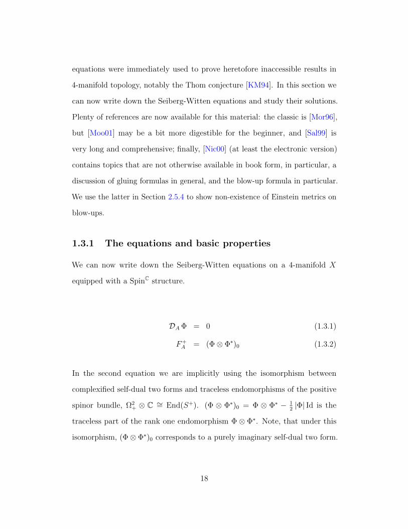
1.3.1 The equations and basic properties

We can now write down the Seiberg-Witten equations on a 4-manifold X

equipped with a SpinC structure.

DA Φ = 0 (1.3.1)

F+A = (Φ⊗ Φ∗)0 (1.3.2)

In the second equation we are implicitly using the isomorphism between

complexified self-dual two forms and traceless endomorphisms of the positive

spinor bundle, Ω2+ ⊗ C ∼= End(S+). (Φ ⊗ Φ∗)0 = Φ ⊗ Φ∗ − 1

2|Φ| Id is the

traceless part of the rank one endomorphism Φ ⊗ Φ∗. Note, that under this

isomorphism, (Φ⊗ Φ∗)0 corresponds to a purely imaginary self-dual two form.

18

It is also necessary to consider the perturbed Seiberg-Witten equations

DA Φ = 0 (1.3.3)

F+A − (Φ⊗ Φ∗)0 = $+ (1.3.4)

where $+ is a self-dual two form.

We can define the Seiberg-Witten map as

SW : A× Γ(S+)→ Ω2+ × Γ(S−) (1.3.5)

SW (A,Φ) =(F+A − (Φ⊗ Φ∗)0,DA Φ

)(1.3.6)

It is important to note that these equations have an infinite dimensional

symmetry group, namely, the group of automorphisms of the principal SpinC-

bundle PCSpin(TM) that cover the identity of the frame bundle PSO(TM) under

π, in the commutative diagram 1.2.1. An automorphism of a SpinC-principal

bundle is given by a smooth map u : M → SpinC. If an automorphism given by

u covers the identity on PSO(TM), then π u : M → SpinC(4)→ SO(4) is the

identity, and so u : M → U(1). Now given a change of gauge u : M → U(1),

(A,Φ) transforms to

u · (A,Φ) = (A− u−1du, uΦ). (1.3.7)

The power of these equations comes from the gained control on the F+A

term in the Weitzenbock formula (1.2.11). Substituting F+A ·Φ = (Φ⊗Φ∗)0Φ =

19

12|Φ|2 Φ into (1.2.11) we obtain

D∗ADAΦ = ∇∗A∇Φ +s

4Φ +

1

4|Φ|2 Φ. (1.3.8)

Note that

〈∇∗A∇AΦ,Φ〉 =1

2∆ |Φ|2 + |∇AΦ|2 . (1.3.9)

So taking the inner product with Φ in (1.3.8), we obtain for a solution of the

Seiberg-Witten equations (1.3.1)

0 = 2∆ |Φ|+ 4 |∇AΦ|2 + s |Φ|2 + |Φ|4 (1.3.10)

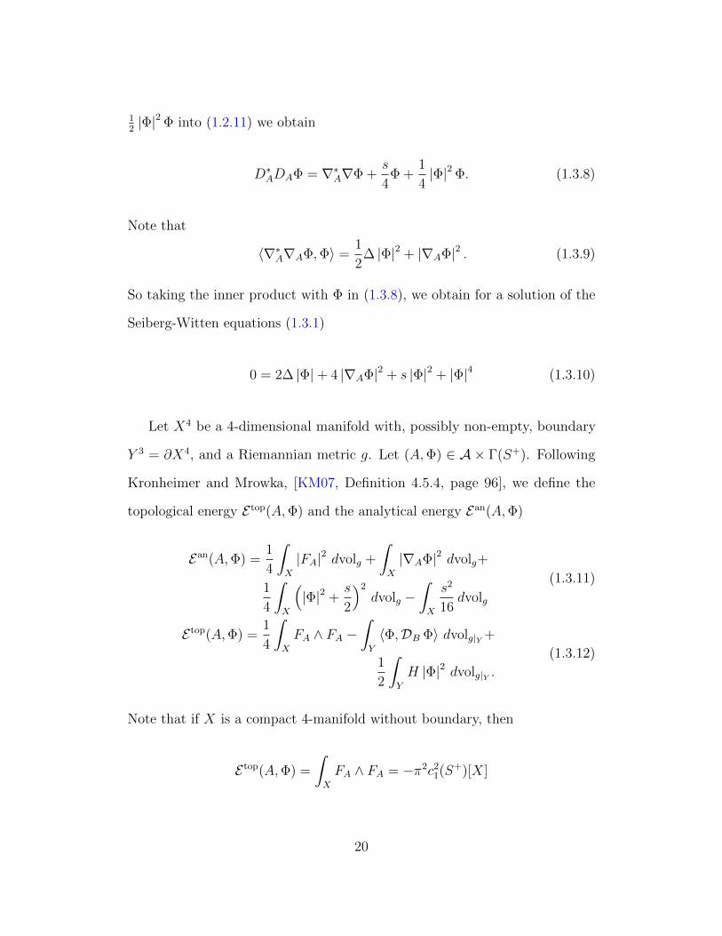
Let X4 be a 4-dimensional manifold with, possibly non-empty, boundary

Y 3 = ∂X4, and a Riemannian metric g. Let (A,Φ) ∈ A × Γ(S+). Following

Kronheimer and Mrowka, [KM07, Definition 4.5.4, page 96], we define the

topological energy E top(A,Φ) and the analytical energy Ean(A,Φ)

Ean(A,Φ) =1

4

∫X

|FA|2 dvolg +

∫X

|∇AΦ|2 dvolg+

1

4

∫X

(|Φ|2 +

s

2

)2

dvolg −∫X

s2

16dvolg

(1.3.11)

E top(A,Φ) =1

4

∫X

FA ∧ FA −∫Y

〈Φ,DB Φ〉 dvolg|Y +

1

2

∫Y

H |Φ|2 dvolg|Y .

(1.3.12)

Note that if X is a compact 4-manifold without boundary, then

E top(A,Φ) =

∫X

FA ∧ FA = −π2c21(S+)[X]

20

is a topological invariant, by Chern-Weil theory.

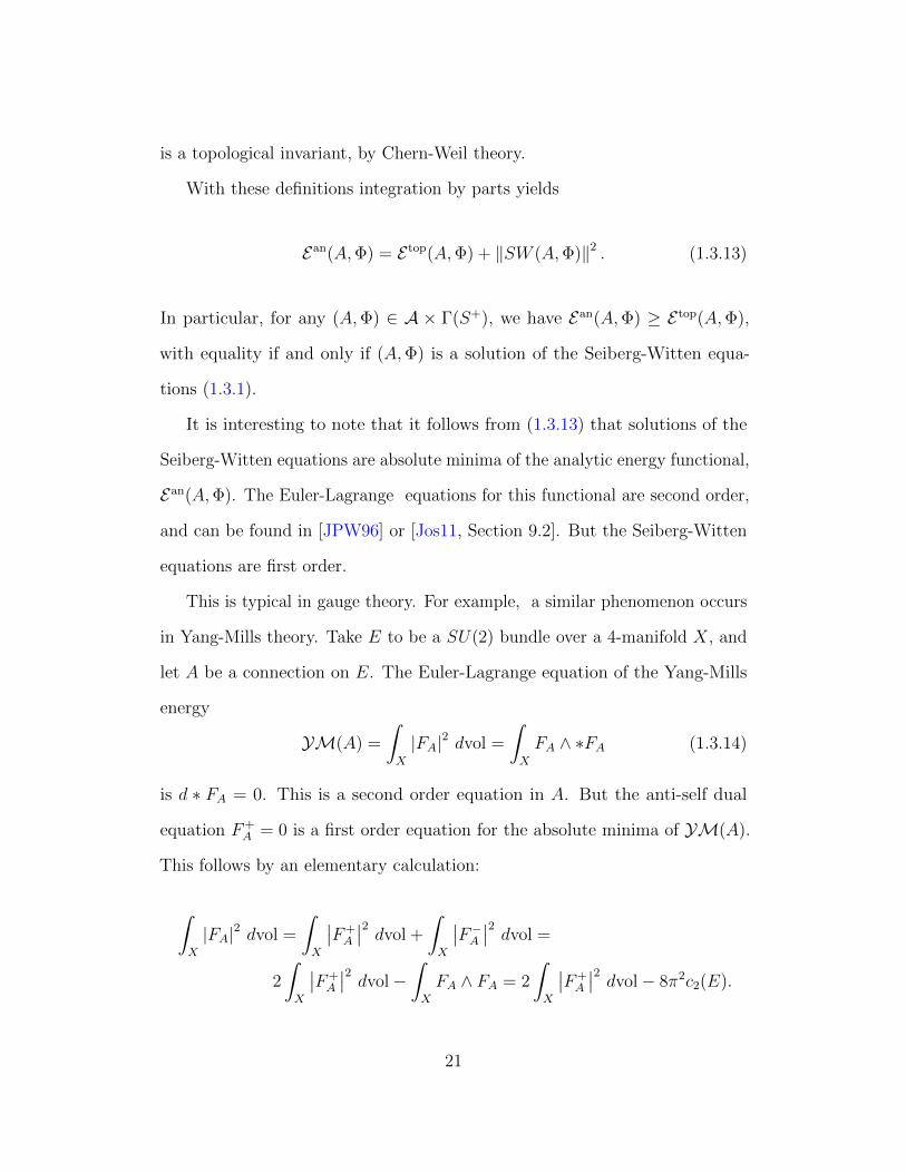
With these definitions integration by parts yields

Ean(A,Φ) = E top(A,Φ) + ‖SW (A,Φ)‖2 . (1.3.13)

In particular, for any (A,Φ) ∈ A × Γ(S+), we have Ean(A,Φ) ≥ E top(A,Φ),

with equality if and only if (A,Φ) is a solution of the Seiberg-Witten equa-

tions (1.3.1).

It is interesting to note that it follows from (1.3.13) that solutions of the

Seiberg-Witten equations are absolute minima of the analytic energy functional,

Ean(A,Φ). The Euler-Lagrange equations for this functional are second order,

and can be found in [JPW96] or [Jos11, Section 9.2]. But the Seiberg-Witten

equations are first order.

This is typical in gauge theory. For example, a similar phenomenon occurs

in Yang-Mills theory. Take E to be a SU(2) bundle over a 4-manifold X, and

let A be a connection on E. The Euler-Lagrange equation of the Yang-Mills

energy

YM(A) =

∫X

|FA|2 dvol =

∫X

FA ∧ ∗FA (1.3.14)

is d ∗ FA = 0. This is a second order equation in A. But the anti-self dual

equation F+A = 0 is a first order equation for the absolute minima of YM(A).

This follows by an elementary calculation:

∫X

|FA|2 dvol =

∫X

∣∣F+A

∣∣2 dvol +

∫X

∣∣F−A ∣∣2 dvol =

2

∫X

∣∣F+A

∣∣2 dvol−∫X

FA ∧ FA = 2

∫X

∣∣F+A

∣∣2 dvol− 8π2c2(E).

21

See [DK90] for an account of the anti-self dual equation, and the four manifold

invariants that arise from it.

To proceed we prove a gauge-fixing lemma. This choice of gauge is known

as Coulomb gauge.

Lemma 1.3.1. Let A0 be a C∞ connection on some Hermitian line bundle on

X. Then for any L2k connection A, there is a L2

k+1 change of gauge u : X → S1,

such that u · A = A0 + α, where α ∈ L2l (T

∗X) and d∗α = 0.

Proof. By (1.3.7), u ·A = A−u−1du, we want to solve d∗(A−A0−u−1du) = 0

for u. Or in other words, d∗(u−1du) = d∗(A − A0) ∈ L2k−1. Now by Hodge

Theory, there is a solution f ∈ L2k+1 to d∗df = d∗(A−A0) (recall the difference

between two connections on a Hermitian line bundle is a purely imaginary

one-form, so f is a purely imaginary function). Let u = ef . Then

d∗(u−1du) = d∗(e−fdef ) = d∗df = d∗(A− A0)

as desired. So the existence of Coulomb gauge is just a consequence of the

solvability of the Poisson equation with right-hand side orthogonal to the locally

constant functions.

Lemma 1.3.2. Let A0, A, α and u be as in the previous lemma. There exists

a constant C such that we can find a further change of gauge v : X → S1 such

that v · A = v · (A0 + α) = A0 + α− v−1dv = A0 + α, with d∗α = 0 and if we

let γ denote the harmonic projection of α, then ‖γ‖L2k< C.

Proof. We can write α = β+γ, where d∗β = d∗γ = dγ = 0 and β is orthogonal

to the harmonic 1-forms. Now suppose γ0 ∈ H1(X) is a harmonic 1-form with

22

periods in 2πZ. In other words, for any loop l : S1 → X,∫lγ0 ∈ 2πZ. Then

there exists a function v0 : X → S1 such that dv0 = γ0. Indeed, after choosing

a basepoint in X, the universal cover of X, integration of the pull-back of γ0 to

X yields a map to iR, v0 : X → iR. Note that dv0 = π∗γ0, where π : X → X.

Since the periods of γ0 are integer multiples of 2π, this map descends to a map

v0 : X → R/2πZ = S1, v0 = exp(v0). By construction, v−10 dv0 = γ0.

Since H1(X)/ γ0 ∈ H1(X) | periods of γ are in 2πZ is a compact torus,

we can write any γ ∈ H1(X) as γ = γ0 + γ1 where γ0 has periods in 2πZ

and ‖γ1‖L2k(X) < C. So we can use v0 constructed above to change gauge to

remove the γ0 term, and we are left with γ = γ1, which has the requisite L2k(X)

bound.

Now we give an argument for the compactness of the space of solutions

to the Seiberg-Witten equations based on an energy bound. This argument

is different from the usual argument, which is based on a C0-bound for the

spinor, which is derived from the Weitzenbock formula, see [Mor96]. However,

this argument is not at all original. For example, a version of this argument for

a manifold with boundary can be found in [KM07]. Further, energy bounds

and compactness, or the lack of compactness, in the case of bubbling, is one of

the most important technical aspects of gauge theory.

The argument below establishes compactness for the space of solutions

modulo gauge to the Seiberg-Witten equations on a closed 4-manifold. Since

the argument is well known, we provide it here since it is a simpler version of

the argument needed to prove Theorem 2.3.1. The main difference is that in

the proof of Theorem 2.3.1, we must consider a sequence of metrics gj , whereas

23

in the current setting, the metric g is fixed.

Proposition 1.3.3. Let s be a SpinC structure, and A0 a fixed smooth connec-

tion on det(s). Let (Aj,Φj) ∈ A× Γ(S+), and SW (A,Φ) = ($+j , 0), for some

perturbations $+j ∈ Ω2

+, with∥∥$+

j

∥∥L21

< C. And assume that Aj = A0 + αj

which αj ∈ L22(Ω1(X)) and Φ ∈ L2

2(S+). Then, there is a sequence of changes

of gauge uj : X → S1, uj ∈ L23, such that uj · (Aj,Φj) has a convergent

subsequence.

Note that the group of L23 changes of gauge is an infinite dimensional Lie

Group thanks to the Sobolev multiplication L23 × L2

3 → L23, and it is thanks

to the Sobolev multiplication L23 × L2

2 → L22 that this Lie Group acts on our

configurations, see A.3.

Before we proceed with the proof of the theorem, we need several Lemmas.

Lemma 1.3.4. Let β ∈ Γ(T ∗X) be a 1-form on a closed Riemannian manifold

(X, g). Suppose β ⊥ H1(X, g). Then

‖β‖L21≤ C (‖dβ‖L2 + ‖d∗β‖L2) . (1.3.15)

Proof. We need to control the L2-norm of the 1-form and its derivative. To

achieve the latter, we note that the Bochner formula for the Hodge laplacian

on 1-forms says

(dd∗ + d∗d)β = ∇∗∇β + Ricg(β, ·)

24

hence,

‖∇β‖2L2 = ‖dβ‖2

L2 + ‖d∗β‖2L2 −

∫X

Ricg(β, β) dvolg

‖∇β‖2L2 ≤ ‖dβ‖2

L2 + ‖d∗β‖2L2 + C ‖β‖2

L2 (1.3.16)

It remains to establish control of the L2-norm of the 1-form itself. Arguing by

contradiction, suppose that the right hand side of (1.3.15) does not control

‖β‖L2 . Then, there exists a sequence βj of 1-forms, orthogonal to H1, with

‖βj‖L2 = 1 and with (‖dβj‖L2 + ‖d∗βj‖L2) → 0. But then (1.3.16) tells us

that ‖βj‖L21< C and so there is a subsequence βjk which weakly converges to

β in L21, and converges strongly in L2. In particular, ‖β‖L2 = 1. But, weak

convergence in L21 implies that dβ = d∗β = 0 so β ∈ H1. On the other hand, β

is also orthogonal to H1, so β = 0, which contradicts ‖β‖L2 = 1.

Proof of Proposition 1.3.3. By equation (1.3.13) we have Ean(Aj,Φj) < C

uniformly in j, and this immediately gives

∥∥FAj

∥∥L2 < C

‖Φj‖L4 < C (1.3.17)∥∥∇AjΦj

∥∥L2 < C all uniformly in j.

By the gauge fixing Lemmas 1.3.1 and 1.3.2 we can assume d∗αj = 0, and

if we write αj = βj + γj where βj is orthogonal to H1(X, g) and γj ∈ H1(X, g),

we can also assume that ‖γj‖L21< C.

Then F+Aj

= F+A0

+ d+βj and since A0 is a fixed connection∥∥F+

A0

∥∥L2 < C

25

uniformly in j. Hence, (1.3.17) gives us ‖d+βj‖L2 < C. But

0 =

∫X

d(β ∧ dβ) =∥∥d+βj

∥∥L2 −

∥∥d−βj∥∥L2 .

Hence, we have ‖dβj‖L2 =√

2 ‖d+βj‖L2 < C. Lemma 1.3.4 then gives us

‖βj‖L21< C. We can pass to a subsequence which converges weakly in L2

1,

βj β ∈ L21. Since ‖γj‖L2

1< C, we can pass to a subsequence which converges

weakly in L21, so γj γ. And hence αj = βj + γj β + β = α converges

weakly in L21. Let A = A0 + α, so Aj converge weakly in L2

1 to A.

Now we establish convergence for the spinor. Equation (1.3.17) gives us an

L4 bound on the spinor and an L2 bound on the covariant derivative of the

spinor, but with a variable connection. We use the following extra argument

to deal with this minor problem. ∇A0Φj = ∇AjΦj − αj ⊗ Φj, so

‖∇A0Φj‖L2 ≤∥∥∇Aj

Φj

∥∥L2 + ‖αj ⊗ Φj‖L2 ≤

C + ‖αj‖L4 ‖Φj‖L4 ≤ C + C ′ ‖αj‖L21‖Φj‖L4 ≤ C ′′

where the first inequality is the triangle inequality, the second inequality is

(1.3.17) and the fact that the L2-norm of the product is controlled by the

product of the L4 norms of the factors by Cauchy-Schwartz, and the third

inequality is the Sobolev embedding L21 → L4 in dimension 4 (see Theorem

A.2). Hence, we have a subsequence Φj weakly convergent in L21, Φj Φ.

After possibly passing to a further subsequence, we then have: FAj, ∇Aj

Φj

and (Φj ⊗ Φ∗j)0 converge weakly in L2, while (Aj,Φj) and the perturbations

$+j $+ converge weakly in L2

1 and hence, strongly in L2. Now, α 7→

26

F+A0+α is a continuous map from L2

1 to L2, and weak convergence is preserved

under continuous maps, hence the weak limit of F+Aj

is F+A . To proceed, we

need to show that the weak limit of ∇AjΦj is ∇AΦ and the weak limit of

(Φj ⊗ Φ∗j)0 is (Φ ⊗ Φ∗)0. Now for the former, note that Aj = A0 + αj so

∇AjΦj = ∇A0Φj + αj ⊗ Φj. Since Φj converges weakly in L2

1 to Φ, ∇A0Φj

converges weakly in L2 to ∇A0Φ. Further, since αj and Φj converge to α and Φ

respectively strongly in L2, αj⊗Φj converges strongly in L1 to α⊗Φ. Similarly,

(Φj ⊗ Φ∗j)0 converges strongly to (Φ⊗ Φ∗)0 in L1 since Φj converges strongly

to Φ in L2. Hence, we can conclude that (A,Φ) solves the Seiberg-Witten

equations, SW (A,Φ) = ($+, 0).

Proposition 1.3.3 says that the set of solutions to the Seiberg-Witten

equations modulo change of gauge is compact. This feature makes Seiberg-

Witten theory considerably simpler than Donaldson’s theory or the theory of

pseudo-holomorphic curves, where solutions can “degenerate” or “bubble,” and

this phenomenon must be understood.

There is actually an L∞ bound for Φ, if (A,Φ) solves the unperturbed

Seiberg-Witten equations.

Proposition 1.3.5. Suppose SW (A,Φ) = 0. Then ‖Φ‖L∞ ≤ max(−s), where

s is the scalar curvature.

Proof. The proof is based on the Weitzenbock formula (1.3.10). Indeed, let

p be a point where |Φ| attains its maximum, then ∆ |Φ|p ≤ 0, so by (1.3.10)

s |Φ|2 + |Φ|4 ≤ 0 and hence, if |Φ|p 6= 0, |Φ|2 ≤ −s ≤ max(−s−), where

f− = min(f, 0), for any function f .

27

1.3.2 The Seiberg-Witten equations on Kahler mani-

folds

On a compact, Kahler manifold, we can directly find the solutions to (1.3.1); in

fact, this computation was done in Section 4 of Witten’s original paper [Wit94],

and [Mor96, Chapter 7] has an excellent discussion, which we follow here.

S+ ∼= Ω0(X;C)⊕ Ω0,2(X;C)

S− ∼= Ω0,1(X;C)

D =√

2(∂ + ∂∗

)where the Dirac operator is for the SpinC-structure associated to the complex

structure and the Chern connection on its determinant line bundle, K−1X .

Φ = (α, β) ∈ Ω0(X;C)⊕ Ω0,2(X;C).

∂A0α + ∂∗β = 0 (1.3.18)

(FA)1,1 =i

4(|α|2 − |β|2)ω (1.3.19)

F 0,2A =

αβ

2(1.3.20)

Theorem 1.3.6. The Seiberg-Witten invariant of a Kahler manifold is non-zero

for the canonical SpinC structure with determinant line bundle the anticanonical

bundle. Therefore, for that SpinC structure, the Seiberg-Witten equations have

a solution on a Kahler manifold with respect to any metric and a generic

perturbation.

28

Chapter 2

Quasiprojective manifolds

Let X be a smooth, projective manifold, D ⊂ X a smooth divisor, and LD its

associated line bundle. Let KX be the canonical bundle and let X = X \D.

Assume that KX ⊗ LD is ample. In [Kob84] it is shown that X admits a

unique, up to scaling, complete Kahler-Einstein metric gKE with negative Ricci

curvature and finite volume.

2.1 Cheng-Yau Holder Spaces

The proof in [Kob84] (also see [TY87] proceeds by using the continuity method

in the Cheng-Yau Holder spaces, introduced in [CY80] by Cheng and Yau to

prove the existence of complete Kahler-Einstein metrics on bounded, strictly

pseudo-convex domains in Cn.

To define the Cheng-Yau Holder spaces we it is first necessary to introduce

“quasi-coordinates.” The model is again the Poincare punctured disk 0 < |z| < 1

29

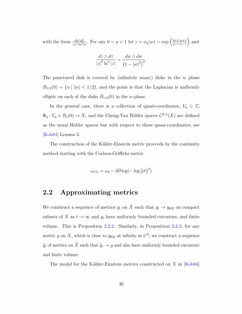
with the form dz∧dz|z|2 ln2|z| . For any 0 < η < 1 let z = φη(w) = exp

(η+1η−1

w+1w−1

)and

dz ∧ dz|z|2 ln2 |z|

=dw ∧ dw(1− |w|2

)2 .

The punctured disk is covered by (infinitely many) disks in the w plane

B1/2(0) = w | |w| < 1/2, and the point is that the Laplacian is uniformly

elliptic on each of the disks B1/2(0) in the w-plane.

In the general case, there is a collection of quasi-coordinates, Vη ⊂ C,

Φη : Vη ×B1(0)→ X, and the Cheng-Yau Holder spaces Ck,λ(X) are defined

as the usual Holder spaces but with respect to these quasi-coordinates, see

[Kob84] Lemma 2.

The construction of the Kahler-Einstein metric proceeds by the continuity

method starting with the Carlson-Griffiths metric

ωCG = ω0 − ∂∂ log(− log ‖σ‖2)

2.2 Approximating metrics

We construct a sequence of metrics gt on X such that gt → gKE on compact

subsets of X as t→∞ and gt have uniformly bounded curvature, and finite

volume. This is Proposition 2.2.2. Similarly, in Proposition 2.2.3, for any

metric g on X, which is close to gKE at infinity in C2, we construct a sequence

gt of metrics on X such that gt → g and also have uniformly bounded curvature

and finite volume.

The model for the Kahler-Einstein metrics constructed on X in [Kob84]

30

is the Poincare metric gH = dz dz|z|2(log |z|)2 on the punctured open disk D =

z | |z| < 1, z 6= 0. As motivation for the construction in Proposition 2.2.2, we

construct a sequence of metrics gt on the unpunctured disk, which converge to gH

on compact subsets of the punctured open disk, have uniformly bounded scalar

curvature, and the volume of a compact subset of the unpunctured open disk

is bounded independent of t. We do this by smoothly transitioning the metric

gH to the flat metric on an annulus of appropriate radius for 1/t2 < |z| < 1/t.

Then we cap off the flat annulus with an appropriate “standard” cap.

Let gE,R = R2 1|z|2dz dz be the flat metric on the punctured plane R2−(0, 0).

Let S1R be a circle of radius R. F : (R2 − (0, 0), gE,R)→ (S1

R ×R, dθ2 + du2),

F (z) = (R arg z,−R ln |z|) is an isometry. Let χ(x) be a smooth function

which satisfies χ(x) = 1 for 0 ≤ x ≤ 1, χ(x) = 0 for 2 ≤ x and is monotonically

decreasing, with χ′(x) and χ′′(x) bounded. Finally, let

gt = (1− χ (− ln |z|/ ln t)) gE,1/ ln t + χ (− ln |z|/ ln t) gH =

1− χ (− ln |z|/ ln t)

|z|2(ln t)2dz dz +

χ (− ln |z|/ ln t)

|z|2(ln |z|)2dz dz =

1

r2

(1− χ) ln2 r + χ ln2 t

ln2 t ln2 rdz dz = f 2dz dz

(2.2.1)

where in the last line we set r = |z|, χ = χ(− ln |z|/ ln t), and the coefficient in

front of dz dz is denoted by f 2 for convenience. gt is equal to gH for |z| > 1/t

and gt is equal to gE,1/ ln t for |z| < 1/t2, and there is a smooth transition region,

Rt = z | 1/t2 < |z| < 1/t. Note that the width, i.e. the distance between

boundary components, of Rt with respect to gH is ln 2, independent of t, and

the width of Rt with respect to gE,1/ ln t is 1, also independent of t. The volume

form of the metric f 2dz dz is i2f 2dz ∧ dz, so the volume (or one might say the

31

area) of Rt with respect to gH is π/ ln t and with respect to gE,1/ ln t is 2π/ ln t.

The scalar curvature of a metric f 2dz dz which is twice the Gaussian

curvature, is (8/f 2) ∂2zz (ln f). So we compute the scalar curvature of gt to

obtain

s = − 2

f 2

(1

r∂r (r∂r ln f) +

1

r2∂2θθ ln f

)=

− ln2 r ln2 t((1− χ) ln2 r + χ ln2 t

)2

(4ρχ′ − ρ2χ′′ + 2(1− χ) + χ′′

)− ln2 r ln2 t(

(1− χ) ln2 r + χ ln2 t)3 ln2 r

(ρχ′ + 2(1− χ)− χ′/ρ

)2

− 2 ln2 t

(1− χ) ln2 r + χ ln2 t

(2.2.2)

where we denote ln r/ ln t by ρ for brevity, and where χ, χ′ and χ′′ are all

evaluated at −ρ. Note that for z ∈ Rt, −2 < ρ < −1. Now let 0 < a ≤ b,

then h(χ) = ab((1−χ)a+χb

)2 is a monotonically decreasing function of χ, which

decreases from b/a to a/b as χ varies from 0 to 1. Hence, by examining (2.2.2)

we see that s is bounded on Rt.

Now to complete the construction, we construct a metric ˜gt on the closed

unit disk. Let ˜gt = gE,1/ ln t for 1/2 < |z| < 1. Let ϕ : z | 1/4 < z < 1/2 →

z | 1/t2 < |z| < 1/2 be a diffeomorphism by scaling radially, and let ˜gt = ϕ∗gt.

Note that for |z| = 1/4, ˜gt(z) = gH(1/2). Finally, let ˜g be an arbitrary metric

on z | |z| ≤ 1/4 that matches gH(1/2) smoothly on the boundary.

The metrics gt and ˜gt glue smoothly on the boundary, since both are equal

to gE,1/ ln t in an open collar around the boundary, yielding a metric gt on

the unpunctured unit disk. By the above computation, scal(gt) is uniformly

bounded, and since gt(z) = gH(z) for |z| > 1/t, gt → gH on compact subsets

32

of D as t→∞. We also have vol(Rt)gt ≤ vol(Rt)gE,1/ ln t+ vol(Rt)gH = 3π/ ln t.

Hence, for K a compact subset of the open, unpunctured disk, vol(K)gt is

uniformly bounded.

Now suppose g is any Riemannian metric on D, which approaches gH in C2

as z → 0. Let

ht = χ (− ln |z|/ ln t) g +(1− χ (− ln |z|/ ln t)

)gH (2.2.3)

This transitions g to gH over the region Rt = z | 1/t2 < |z| < 1/t as before.

scalht is uniformly bounded on Rt, and vol(Rt)ht is uniformly bounded as well.

This motivates a similar construction in the quasiprojective case. The

construction is possible, thanks to the asymptotics of gKE found in [Sch98]. For

the convenience of the reader, we quote the asymptotics from [Sch98, Sch02]:

Theorem 2.2.1 (Schumacher 1998). Let σ be a suitably chosen section of LD,

defining D, and ‖·‖ a suitably chosen Hermitian metric on LD. In suitable local

coordinates (σ, z), ωKE, the Kahler form associated to gKE has the following

asymptotics:

ωKE =

(2h

‖σ‖2 (log ‖σ‖)2

(1 +

µ

(log ‖σ‖)α

))dσ ∧ dσ+

O

(1

‖σ‖ (log ‖σ‖)1+α

)dσ ∧ dz +O

(1

‖σ‖ (log ‖σ‖)1+α

)dσ ∧ dz+

fdz ∧ dz (2.2.4)

where fdz∧dz converges to the Kahler-Einstein metric on D and µ ∈ Ck,λ(X).

These asymptotics are restated as follows in [Sch02]. Let z1 = σ, and

33

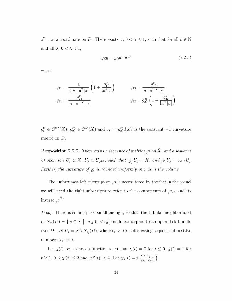
z2 = z, a coordinate on D. There exists α, 0 < α ≤ 1, such that for all k ∈ N

and all λ, 0 < λ < 1,

gKE = gidzidz (2.2.5)

where

g11 =1

2 |σ| ln2 |σ|

(1 +

g011

lnα σ

)g12 =

g012

|σ| ln1+α |σ|

g21 =g0

21

|σ| ln1+α |σ|g22 = g∞22

(1 +

g022

lnα |σ|

)

g0i ∈ Ck,λ(X), g∞22 ∈ C

∞(X) and gD = g∞22dzdz is the constant −1 curvature

metric on D.

Proposition 2.2.2. There exists a sequence of metrics gj on X, and a sequence

of open sets Uj ⊂ X, Uj ⊂ Uj+1, such that⋃j Uj = X, and gj |Uj = gKE|Uj.

Further, the curvature of gj is bounded uniformly in j as is the volume.

The unfortunate left subscript on gj is necessitated by the fact in the sequel

we will need the right subscripts to refer to the components of gj αβ

and its

inverse gβαj

Proof. There is some ε0 > 0 small enough, so that the tubular neighborhood

of Nε0(D) =p ∈ X

∣∣ ‖σ(p)‖ < ε0

is diffeomorphic to an open disk bundle

over D. Let Uj = X \Nεj(D), where εj > 0 is a decreasing sequence of positive

numbers, εj → 0.

Let χ(t) be a smooth function such that χ(t) = 0 for t ≤ 0, χ(t) = 1 for

t ≥ 1, 0 ≤ χ′(t) ≤ 2 and |χ′′(t)| < 4. Let χj(t) = χ(t−εj+1

εj−εj+1

).

34

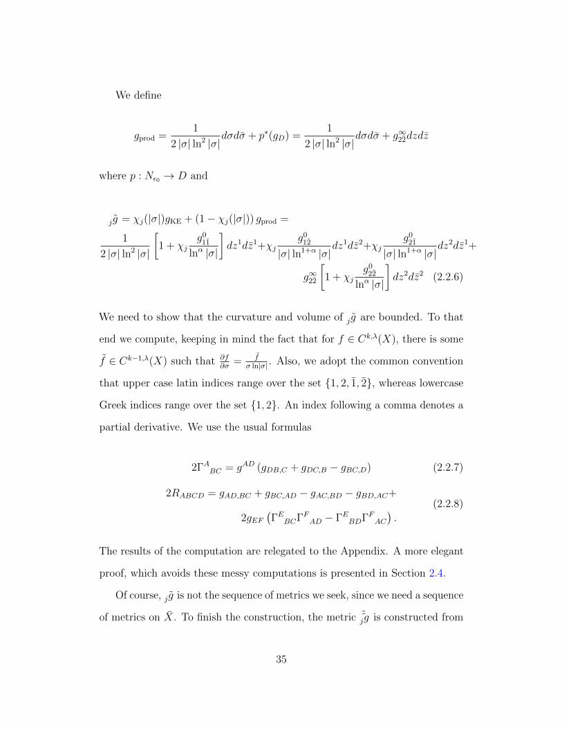
We define

gprod =1

2 |σ| ln2 |σ|dσdσ + p∗(gD) =

1

2 |σ| ln2 |σ|dσdσ + g∞22dzdz

where p : Nε0 → D and

gj = χj(|σ|)gKE + (1− χj(|σ|)) gprod =

1

2 |σ| ln2 |σ|

[1 + χj

g011

lnα |σ|

]dz1dz1+χj

g012

|σ| ln1+α |σ|dz1dz2+χj

g021

|σ| ln1+α |σ|dz2dz1+

g∞22

[1 + χj

g022

lnα |σ|

]dz2dz2 (2.2.6)

We need to show that the curvature and volume of gj are bounded. To that

end we compute, keeping in mind the fact that for f ∈ Ck,λ(X), there is some

f ∈ Ck−1,λ(X) such that ∂f∂σ

= fσ ln|σ| . Also, we adopt the common convention

that upper case latin indices range over the set 1, 2, 1, 2, whereas lowercase

Greek indices range over the set 1, 2. An index following a comma denotes a

partial derivative. We use the usual formulas

2ΓABC = gAD (gDB,C + gDC,B − gBC,D) (2.2.7)

2RABCD = gAD,BC + gBC,AD − gAC,BD − gBD,AC+

2gEF(ΓEBCΓFAD − ΓEBDΓFAC

).

(2.2.8)

The results of the computation are relegated to the Appendix. A more elegant

proof, which avoids these messy computations is presented in Section 2.4.

Of course, gj is not the sequence of metrics we seek, since we need a sequence

of metrics on X. To finish the construction, the metric ˜gj is constructed from

35

gj by transitioning the “Poincare” factor 1/2 |σ| ln2 |σ| to a cylindrical metric as

in the discussion at the beginning of the Section. To complete the construction

of the metric compactification, we take Nε0(D)\Nεj+1, with the cylindrical end,

and glue it back on to Uj+1 with its cylindrical end. Then, we can smoothly

cap off Nε0(D) with an arbitrary metric on the total space of the disk bundle

Nε0(D) which is fixed once and for all throughout the construction.

Proposition 2.2.3. Let g be a metric on X which is C2 close to gKE at

infinity. In other words, for any ε > 0, there is a compact set K ⊂ X, such

that ‖g − gKE‖C2(X\K,gKE) < ε. Then there exists a sequence of metrics gj on

X, and a sequence of open sets Uj ⊂ X, Uj ⊂ Uj+1, such that⋃j Uj = X, and

gj|Uj = g|Uj.

Proof. Take χj and Uj as above. And let gj = χj(|σ|)g+(1−χj(|σ|))gKE. We get

a sequence of metrics such that gj|Uj = g|Uj and gj|(X\Uj+1) = gKE|(X\Uj+1).

Now we can approximate gj by a metric gj on X as in Proposition 2.2.2.

2.3 Existence theory for the Seiberg-Witten

equations

We follow Biquard’s argument [Biq97] and produce an irreducible solution to

the Seiberg-Witten equations (1.3.1) on (X, g) by considering a sequence of

solutions to the perturbed equations on (X, gj), where the gj are the approxi-

mating metrics obtained in Proposition 2.2.3. This argument was also used by

Rollin [Rol02] and Di Cerbo[DC11, DC12].

36

Theorem 2.3.1. As throughout this Chapter, let X be a smooth, projective

manifold, b2+(X) ≥ 2, D ⊂ X a smooth divisor, and LD its associated line

bundle. Let KX be the canonical bundle and let X = X \ D. Assume that

KX ⊗ LD is ample. Let gKE be the unique complete Kahler-Einstein metric of

Ricci curvature −1. Let g be any metric that is C2 close to gKE at infinity as

in Proposition 2.2.3. Then there exists an irreducible ( i. e. Φ 6≡ 0) solution

(A,Φ) ∈ A × S+ on (X, g) in the SpinC structure s which is the restriction

to X of the SpinC structure on X with determinant line bundle KX . Further,

if A0 is a fixed C∞ connection on X, then A = A0 + α, where α ∈ Γ(T ∗X),

α ∈ L21(X, g) and d∗α = 0. Further, sup ‖Φ‖ < C..

The condition b2+(X) ≥ 2 can be relaxed to b2

+(X) ≥ 1, however, we then

need to keep track of chambers in working with the Seiberg-Witten invariant.

Before we proceed with the proof of the theorem, we need several Lemmas.

Lemma 2.3.2. Let β ∈ Γ(T ∗M) be a 1-form on a closed Riemannian manifold

(M, g). Suppose β ⊥ H1(M, g). Then

‖β‖L21(M,g) ≤ C

(‖dβ‖L2(M,g) + ‖d∗β‖L2(M,g)

). (2.3.1)

Proof. We need to control the L2-norm of the 1-form and its derivative. To

achieve the latter, we note that the Bochner formula for the Hodge Laplacian

on 1-forms says

(dd∗ + d∗d)β = ∇∗∇β + Ricg(β, ·)

37

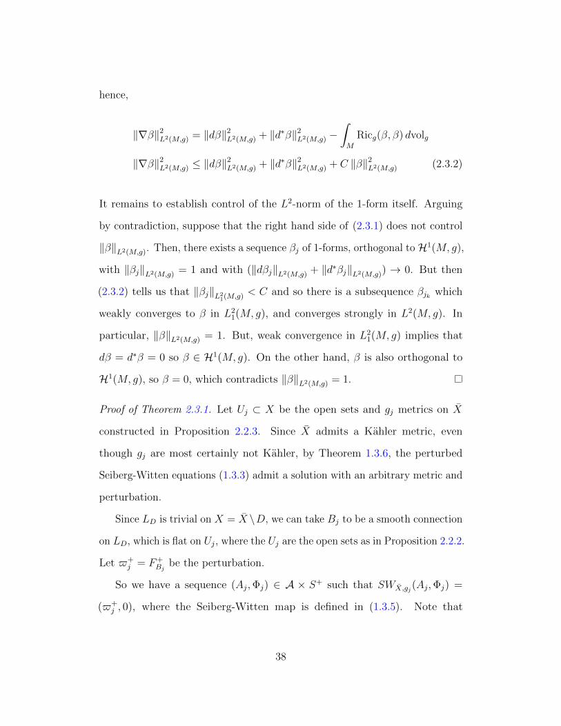
hence,

‖∇β‖2L2(M,g) = ‖dβ‖2

L2(M,g) + ‖d∗β‖2L2(M,g) −

∫M

Ricg(β, β) dvolg

‖∇β‖2L2(M,g) ≤ ‖dβ‖

2L2(M,g) + ‖d∗β‖2

L2(M,g) + C ‖β‖2L2(M,g) (2.3.2)

It remains to establish control of the L2-norm of the 1-form itself. Arguing

by contradiction, suppose that the right hand side of (2.3.1) does not control

‖β‖L2(M,g). Then, there exists a sequence βj of 1-forms, orthogonal to H1(M, g),

with ‖βj‖L2(M,g) = 1 and with (‖dβj‖L2(M,g) + ‖d∗βj‖L2(M,g)) → 0. But then

(2.3.2) tells us that ‖βj‖L21(M,g) < C and so there is a subsequence βjk which

weakly converges to β in L21(M, g), and converges strongly in L2(M, g). In

particular, ‖β‖L2(M,g) = 1. But, weak convergence in L21(M, g) implies that

dβ = d∗β = 0 so β ∈ H1(M, g). On the other hand, β is also orthogonal to

H1(M, g), so β = 0, which contradicts ‖β‖L2(M,g) = 1.

Proof of Theorem 2.3.1. Let Uj ⊂ X be the open sets and gj metrics on X

constructed in Proposition 2.2.3. Since X admits a Kahler metric, even

though gj are most certainly not Kahler, by Theorem 1.3.6, the perturbed

Seiberg-Witten equations (1.3.3) admit a solution with an arbitrary metric and

perturbation.

Since LD is trivial on X = X \D, we can take Bj to be a smooth connection

on LD, which is flat on Uj , where the Uj are the open sets as in Proposition 2.2.2.

Let $+j = F+

Bjbe the perturbation.

So we have a sequence (Aj,Φj) ∈ A × S+ such that SWX,gj(Aj,Φj) =

($+j , 0), where the Seiberg-Witten map is defined in (1.3.5). Note that

38

∥∥$+j

∥∥L21(X,gj)

< C uniformly in j. By equation (1.3.13) we then get

EanX,gj

(Aj,Φj) < C uniformly in j, and this immediately gives

∥∥FAj

∥∥L2(X,gj)

< C

‖Φj‖L4(X,gj) < C∥∥∇AjΦj

∥∥L2(X,gj)

< C all uniformly in j.

Now let us write Aj = A0 + αj, by the gauge fixing Lemma 1.3.1 we can

assume d∗jαj = 0, where d∗j is the adjoint of the exterior derivative with respect

to gj , and by the Hodge decomposition we can further write αj = βj +γj where

βj is orthogonal to H1(X, gj) and γj ∈ H1(X, gj). Further, we can assume that

‖γj‖ < C.

Then F+Aj

= F+A0

+d+βj and since A0 is a fixed connection∥∥F+

A0

∥∥L2(X,gj)

< C

uniformly in j. Hence, (1.3.17) gives us ‖d+βj‖L2(X,gj) < C. But

0 =

∫X

d(β ∧ dβ) =∥∥d+βj

∥∥L2(X,gj)

−∥∥d−βj∥∥L2(X,gj)

. (2.3.3)

Hence, we have ‖dβj‖L2(X,gj) =√

2 ‖d+βj‖L2(X,gj) < C. Lemma 2.3.2 then gives

us ‖βj‖L21(X,gj) < C. By a diagonal argument, we can pass to a subsequence

which converges weakly in L21(X, g), βj β ∈ L2

1(X, g). Indeed, firstly, recall

that by the construction in Proposition 2.2.3, gj|Uj = g|Uj. So ‖βj‖L21(Uk,g)

=

‖βj‖L21(Uk,gk) ≤ ‖βj‖L2

1(X,gk) < C. Define β1,j as a subsequence of βj which

converges weakly in L21(U1, g). Then assuming that for k ≥ 1, βk,j converges

weakly in L21(Uk, g), define βk+1,j as a subsequence of βk,j which converges

weakly in L21(Uk+1, g). Then a subsequence of βj,j β ∈ L2

1(X, g), converges

39

weakly as claimed.

Now we establish convergence for the spinor. (1.3.17) gives us an L4 bound

on the spinor and an L2 bound on the covariant derivative of the spinor, but

with a variable connection, and a variable metric so we need the following extra

argument. ∇A0Φj = ∇AjΦj − αj ⊗ Φj, so

‖∇A0Φj‖L2(X,gj) ≤∥∥∇Aj

Φj

∥∥L2(X,gj)

+ ‖αj ⊗ Φj‖L2(X,gj) ≤

C + ‖αj‖L4(X,gj) ‖Φj‖L4(X,gj) ≤ C + C ′ ‖αj‖L21(X,gj) ‖Φj‖L4(X,gj) ≤ C ′′ (2.3.4)

where the first inequality is the triangle inequality, the second inequality is

(1.3.17) and the fact that the L2-norm of the product is controlled by the

product of the L4 norms of the factors by Cauchy-Schwartz, and the third

inequality is the Sobolev embedding L21 → L4 in dimension 4 (see Theorem

A.2). A diagonalization argument, just as for the 1-forms above, now gives us

a subsequence Φj weakly convergent in L21(X, g).

2.4 Alternate Approach to Existence of Solu-

tions of the Seiberg-Witten equtions

In this section we present an alternative proof of Theorem 2.3.1. Instead of

approximating gKE, the Kahler-Einstein metric on X = X \D, by a smooth

sequence of metrics on X, we approximate gKE by a sequence of orbifold Kahler-

Einstein metrics with orbifold singularity of cone angle 2πβ along D, with

β = 1/p, p ∈ N, β → 0.

40

The definition of an orbifold with singularity along a surface, a review of

differential topology and Hodge theory on orbifolds, and most importantly,

the definition of the Seiberg-Witten invariant in this context, can be found in

[LeB13a]. For the convenience of the reader we quote some of the necessary

results and definitions here. Given X, a smooth, compact 4-manifold, and

D ⊂ X, a smoothly embedded surface, and β = 1/p, an orbifold (X,D, β) is

defined as follows. Near any point q ∈ D, there is a coordinate neighborhood

Uα with coordinates (wα, zα), where U ∩D = (wα, zα) | zα = 0 , and we have

Uα → Uα, (w, ζ) 7→ (w, ζp/ ‖ζ‖p−1). The action on ζ is the standard isometric

Zp action on R2 ∼= C. Uα is an orbifold chart. The transition functions must lift

as diffeomorphisms of R4. In [LeB13a] this is referred to as the “origami” model.

The model more frequently used in holomorphic geometry, is (w, ζ) 7→ (w, ζp).

These two models are related by an appropriate homeomorphism of X to istelf,

which is homotopic to the identity, and differs from the identity only in a

tubular neighborhood of D. Note that ordinarily, an orbifold is defined more

generally, where the finite group may vary from orbifold chart to orbifold chart,

there is no restriction on dimension, and one uses real coordinates rather than

complex ones. However, we state the definition for the application in the sequel.

A smooth object, such as a metric, or a differential form is smooth on the

orbifold (X,D, β), if it is smooth in the orbifold charts Uα and Zp-invariant.

A crucial further concept is one of V -bundle, which is a total space E,

with a projection p : E → X, however, unlike the smooth case, in the orbifold

case the projection is not required to be locally trivial. Rather, we require

that for some fixed vector space, V , there is a system of orbifold charts, such

that there is an isomorphism p−1(Uα)→ (Uα × V )/Zp, where the action of Zp

41

on Uα is the given orbifold action, and the action on V is some linear action.

The transition functions on the overlaps are required to act linearly, as in the

smooth case. Note, however, that the fiber over a singular point may be a

quotient of V . The definition of sections of V -bundles, as well as tensor and

exterior products carry over from the smooth case. A connection on a V -bundle

E is a map ∇ : Γ(E,U) → Γ(E ⊗ T ∗X, U) for any open set U ⊂ X. In our

setting, the finite groups figuring in the definition of orbifold, is Zp over every

singular point. Hence, since L⊗p is then locally trivial, we can define, as in

[LeB13a], corb1 (L) = 1

pc1(L⊗p) ∈ H2(X,Q). The deRham theory and the Hodge

Theorem carry over to this context, as does the Chern-Weil theorem that for

a connection ∇, [ i2πF∇] = corb

1 (L), for a line V -bunlde L, a connection ∇ on

L, and F∇ its curvature. The reader not familiar with these in the orbifold

setting is referred to Section 2 of [LeB13a].

The Seiberg-Witten invariant, in this context is defined assuming X is

almost complex and D is a pseudo-holomorphic curve. The definition of the

Seiberg-Witten invariant in this setting, can be found in Sections 2.4, 2.5, 2.6

and 3 of [LeB13a]. We summarize this construction in the discussion below.

First, we quote the following proposition,

Proposition 2.4.1 ([LeB13a], pg. 17). Let X, D, β be as above: X a smooth,

almost complex 4-manifold, with almost complex structure J0, D ⊂ X a pseudo-

holomorphic curve (with respect to J0), and β = 1/p, p ∈ N, p ≥ 2. Then,

there exists an almost complex structure J on X, which is homotopic to J0,

coincides with J0 along D and outside a tubular neighborhood of D, and is

integrable in a tubular neighborhood of D.

42

This allows us to associate to an almost-complex structure J0 on X, which

by the above without loss of generality we can assume integrable in a tubular

neighborhood of D, an orbifold almost complex structure J on (X,D, β). On

X = X \D, J is simply J0, and on orbifold charts (in the holomorphic geometry

model) around points of D, we take J to be the usual complex structure, with

respect to the orbifold charts. J can also be understood in the usual orbifold

charts (the “origami” model), as is explained in [LeB13a].

Making the almost complex structure integrable in a tubular neighborhood

of D, and working in the holomorphic geometry model, allows one to prove

corb1 (X, J0, D, β) = c1(X, J0) + (β − 1)[D], β = 1/p, p ∈ N

Now, as in Example 1.2.5, outside a tubulur neighborhood of D, the almost

complex structure J determines a SpinC structure s with determinant line

bundle L = det s = Λ0,2. Using the holomorphic geometry model, this can be

extended to the orbifold setting, though now, the bundles Λp,q are V -bundles.

In particular, the SpinC-V -bundles of spinors, just as in the smooth case, are

S+ = Λ0,0 ⊕ Λ0,2 and S− = Λ0,1. If the orbifold metric is Kahler and we take

the Chern connection on L = detS+ = detS− = K−1, then the associated

SpinC-Dirac operator is D =√

2(∂ + ∂∗). The Dirac operator for more general

metrics will differ from the latter by a 0th-order term, and hence, have the

same principal symbol, and hence the same index. The latter can be computed

in the holomorphic geometry model and is 14(χ + σ), where χ is the Euler

characteristic of X and σ is the signature, same as in the smooth case. Note

that in our application, X is a complex manifold, and D is a divisor.

43

With spinors and the Dirac operator carried over to the orbifold setting we

can write down the Seiberg-Witten equations. Note, that the special choice of

orbifold-(almost)-complex structure on (X,D, β), and the resulting choice of

SpinC structure s on the orbifold, is key to computing the index of the Dirac

operator D on the orbifold to be the same as on X, 14(χ+ σ). We then have

the following orbifold version of the Seiberg-Witten invariants, developed in

[LeB13a].

Theorem 2.4.2 ([LeB13a], Proposition 3.2). Let (X, J0) be almost complex,

D ⊂ X a pseudo-holomorphic curve, p ∈ N, p ≥ 2, β = 1/p. Equip the orbifold

(X,D, β) with the orbifold almost complex structure J and corresponding SpinC

structure as in the discussion above. Then for any orbifold metric g, and generic

perturbation $+ the space of solutions to the perturbed Seiberg-Witten equations,

modulo gauge equivalence, is finite. Further, if b+(X) ≥ 2, then the two spaces

of solutions modulo gauge for different choices of metric and perturbation are

cobordant. This allows us to define the mod-2 Seiberg-Witten invariant of

(X,D, β) as the mod-2 count of points in the space of solutions module gauge,

with respect to any metric, and generic perturbation (the perturbations simply

need to be a regular value of the SW map.

Note that if the Seiberg-Witten invariant is non-zero, the above implies the

existence of solutions for any metric and perturbation. Indeed, if there were

no solutions for some perturbation, this perturbation would be a regular point,

and we could use it to compute the invariant, and conclude that it is 0. Of

course, we are not saying that one can use any perturbation to compute the

invariant. Merely, that a solution must exist for any perturbation.

44

The invariant would not be terribly useful, if the non-vanishing results

did not also carry over to the orbifold setting, but fortunately, they do, and

we have the orbifold version of Taubes famous non-vanishing result of the

Seiberg-Witten invariant

Theorem 2.4.3 (Taubes). In the setting of Theorem 2.4.2, let us assume that

X is actually a symplectic orbifold with symplectic form ω, J0 is compatible

with the symplectic structure, and ω restricts as an area form to D. Then,

if b+(X) ≥ 2, the Seiberg-Witten invariant of X, with respect to the SpinC

structure associated to J as above, is non-zero.

Theorems 2.4.2 and 2.4.3 imply the following existence theorem, which we

need to start the proof of Theorem 2.3.1.

Theorem 2.4.4. Let X be a smooth, compact, Kahler 4-manifold, b+ ≥ 2,

D ⊂ X a smooth divisor, p ∈ N, p ≥ 2, β = 1/p. Then for any orbifold metric

g on X, and with the SpinC structure s as above, there exists a solution to the

Seiberg-Witten equations with arbitrary perturbation.

In addition to the above theory of the Seiberg-Witten equations on almost

Kahler manifolds with orbifold singularities along a surface, the other crucial

ingrdient in the proof of existence is an approximation of the Kahler-Einstein

metric gKE on X = X \ D by orbifold, Kahler-Einstein metrics on X with

orbifold singularity along D. This approximation is furnished by the following

theorem due to Henri Guenancia [Gue].

Theorem 2.4.5 (Henri Guenancia). Let X be a smooth, projective complex

manifold, and D a smooth divisor such that KX ⊗ LD > 0. Then there is a

45

sequence of Kahler-Einstein, orbifold metrics gj on X with conical singularity

along D, with cone angle βj going to 0, and gj → gKE on compact subsets of

X = X \D.

Note, that this theorem provides a sequence of Kahler-Einstein conical

metrics; whereas, for our purposes it would be sufficient to have a sequence of

conical metrics, which are merely Kahler, and have Ricci curvature uniformly

bounded below. These can be constructed directly, but instead we quote

Guenancia’s much more powerful result above.

With the approximating conical metrics in hand, we can proceed with the

alternate proof of existence. Firstly, we note that the Poincare type lemma

for 1-forms, Lemma 2.3.2 and the Gauge fixing lemma, Lemma 1.3.2 apply

in the orbifold setting. Indeed, the Poincare type lemma is proved by the

Bochner formula and integration by parts, both of which carry over to the

orbifold setting. The Gauge fixing lemma is proved by Hodge theory, which

again carries over to orbifolds.

Now we can proceed to the proof of existence of solutions to the Seiberg-

Witten equations (1.3.1) on X, with respect to any metric g which is C2-close

to gKE at infinity, Theorem 2.3.1.

Proof of existence. Let gj be the conical KE metrics furnished by Theorem 2.4.5

(decorated with a tilde, since we reserve the designation gj for metrics that we

will construct momentarily). Now let Uj ⊂ X be a sequence of open sets, with⋃Uj = X, Uj ⊂ Uj+1. For definiteness, we can let Uj = ‖s‖ > 1/j , where s

is a defining section for D. Then let χj be a smooth function on X, such that

χj(q) = 1 for q ∈ Uj and χj(q) = 0 for q ∈ Uj+2. Let gj = χjg + (1 − χj)gj.

46

These gj are orbifold metrics on X, which converge to g on compact subsets of

X. Theorem 2.4.4 then furnishes us with an irreducible solution (Aj,Φj) of

the Seiberg-Witten equations with respect to the conical metric gj. Note, that

here Aj is a connection on the V -bundle det(s), where s is the SpinC structure

described above, and Φj ∈ Γ(S+) is a spinor, but also on the orbifold.

Now, just as in the case of a smooth compactification, the solutions have

uniform apriori bounds (1.3.17), namely L2 bounds on the curvature of A, L4

bounds on the spinor Φ, and an L2 bound on∥∥∇Aj

Φj

∥∥L2(X,gj)

. Indeed, these

bounds are a consequence of (1.3.13), which is obtained by integrating by parts

‖SW (Aj,Φj)‖2L2(X,gj). Since Stoke’s Theorem holds for orbifolds, so does the

relation (1.3.13)

EanX,gj

(Aj,Φj) =1

4

∫X

∣∣FAj

∣∣2 dvolg+

∫X

∣∣∇AjΦj

∣∣2 dvolgj+1

4

∫X

(|Φj|2 +

sj2

)2

dvolgj

−∫X

s2j

16dvolgj = E top

X,gj(Aj,Φj) + ‖SW (Aj,Φj)‖2

L2(X,gj) =

1

4

∫X

FAj∧ FAj

+ ‖SW (Aj,Φj)‖2L2(X,gj) .

If SW (Aj,Φj) = $+j , where $+

j is a sequence of perturbations bounded in L2,∥∥$+j

∥∥L2(X,gj)

< C, then we obtain the a priori bounds claimed above. These a

priori bounds, in turn, imply compactness, just as in the smooth case.

Indeed, by the Gauge-Fixing Lemma, if we fix a smooth orbifold connection

A0, then Aj = A0 + αj, and we can assume d∗αj = 0, i. e. we are in Coulomb

gauge. Further, just as in the smooth case, a further change of gauge allows us

to assume that not only d∗αj = 0, but αj = βj + γj, where βj is orthogonal

to H1(X, gj) and γj ∈ H1(X, gj) and ‖γj‖L21< C. Now, F+

Aj= F+

A0+ d+βj,

47

and hence, the uniform L2 bounds on the curvature FAjgives us uniform

bounds on ‖d+βj‖. Since Stokes Theorem holds for orbifolds, equation (2.3.3)

also holds on the orbifold, and we obtain a bound on ‖dβj‖L2(X,gj). Finally,

the Poincare Lemma, then gives us a uniform bound on ‖βj‖L21(X,gj). The

same diagonal argument as in the smooth case allows us to extract a weakly

convergent in L21(X, g) subsequence, which by abuse of notation, we continue

to call βj β. Now, (2.3.4) holds on the orbifold as well, which along with

the discussion which follows this equation in the smooth case gives convergence

on a subsequence for the spinor as well.

Solutions of the Seiberg-Witten equations are actually smooth, as can be

shown by standard elliptic bootstrapping.

We will also need the following classical C0 bound for the spinor.

Proposition 2.4.6. Let (A,Φ) be a solution of the Seiberg-Witten equations

on (X, g). Then ‖Φ‖L∞ ≤ supX −s−, where s− = min(s, 0), where s is the

scalar curvature of g.

Proof. We have equation (1.3.10)

It remains to show that the solution obtained is irreducible, which we do in

the following proposition:

Proposition 2.4.7. The solution obtained above is irreducible, i. e. Φ 6≡ 0.

Proof. First, we need the following uniform lower bound on the L4 norm of

48

the spinor on X.

0 < 4π2c21(KX⊗LD) =

∫X

FAj∧FAj

=

∫X

∣∣∣F+Aj

∣∣∣2 dvolgj−∫X

∣∣∣F−Aj

∣∣∣2 dvolgj =

const ‖Φj‖4L4(X,gj) −

∥∥∥F−Aj

∥∥∥2

L2(X,gj). (2.4.1)

Hence,

0 < δ +1

C

∥∥∥F−Aj

∥∥∥2

L2(X,gj)< ‖Φj‖4

L4(X,gj) .

Let Nj(D) = p ∈ X | ‖σ(p)‖ < ε0 for σ a defining section for D, and let

Uj = X \Nj(D). So that X = Nj

⋃Uj. Then we have

‖Φj‖4L4(Uj ,gj) = ‖Φj‖4

L4(X,gj)−‖Φj‖4L4(Nj(D),gj) ≥ δ−max(s−) vol(Nj(D), gj) > δ/2,

for j sufficiently large, where we used Proposition 2.4.6 for the uniform L∞

bound on the spinor. Thus, we have a uniform lower bound on the L4 norm of

the spinors on Uj, and the proposition follows.

49

2.5 Geometric Consequences

2.5.1 L2-cohomology

To obtain geometric consequences for the existence of solutions to the Seiberg-

Witten equations, we need to quote some facts about L2-cohomology of complete

manifolds. Our exposition follows [Car02, And88].

Let (X, g) be a complete, oriented Riemannian manifold. Let ΩkL2(g) be the

Hilbert completion of the space of smooth k-forms on X such that∫Xα∧∗gα <

∞ with respect to the inner product 〈α, β〉 =∫Xα∧∗gβ. The maximal domain

of the exterior derivative dk on k-forms is defined as

Dk =α ∈ Ωk

L2(g)

∣∣∣ dα ∈ Ωk+1L2(g)

so we have

dk : Dk → Im dk ⊂ Ωk+1L2(g)

and the reduced L2-cohomology groups are defined as usual as the quotient of

the closed forms by the closure of the coboundaries:

HkL2(g) =

α ∈ Ωk

L2(g)

∣∣∣ dkα = 0

Im dk−1

.

Note that under the assumption that X is complete, Im dk−1 is the equal to

the closure of the image of d applied to compactly supported smooth forms.

Further, the harmonic forms are defined as usual as well

Hkg =

α ∈ Ωk

L2(g)

∣∣∣ dα = 0, d∗α = 0

=α ∈ Ωk

L2(g)

∣∣∣ (dd∗ + d∗d)α = 0

50

The Hodge decomposition carries over to this setting:

ΩkL2(g) = Hk

g ⊕ Im dk−1 ⊕ Im d∗gk+1

and so

HkL2(g) = Hk

g .

The Hodge star realizes the Poincare duality isomorphism ∗g : Hkg → Hn−k

g ;

and moreover, if the dimension of X is a multiple of 4, then the Hodge star gives

an isomorphism ∗g : ΩdimX/2

L2(g) → ΩdimX/2

L2(g) which squares to 1. The self-dual and

anti-self-dual forms are then the +1 and the −1 eigenspaces of ∗g on ΩdimX/2

L2(g) .

If HdimX/2g is finite-dimensional, then the difference of the dimensions of the

self-dual and anti-self-dual subspaces is the L2-signature.

Now let L be a line bundle on X, and let (X, g) be a finite volume 4-

manifold. Let A be a connection L, such that FA ∈ Ω2L2(g). Chern-Weil theory

extends to this situation, and we can define c1(L) = i2π

[FA] ∈ H2L2(g). If B is a

different connection, such that α = B − A ∈ D1 ⊂ Ω1L2(g), then FB = FA + dα

and so [FB] = [FA] ∈ H2L2(g). Hence, the L2-Chern class is independent of the

connection, as long as the connections only differ by L2 1-forms in the closure

of the domain of d. Further,

Lemma 2.5.1. c21(L) =

∫XFA ∧ FA is also independent of the connection.

51

Proof.

∫X

FB∧FB =

∫X

(FA+dα)∧(FA+dα) =

∫X

FA∧FA+

∫X

2dα∧FA+dα∧dα =∫X

FA ∧ FA +

∫X

d (α ∧ (2FA + dα)) =

∫X

FA ∧ FA.

Proposition 2.5.2. Let L be a line bundle on (X, g), a finite-volume 4-

manifold, and A a connection on L with FA ∈ Ω2L2(g). Then

∫X

∣∣F+A

∣∣2 dvolg ≥ 4π2(c+1 (L))2

Proof. Since FA ∈ Ω2L2(g), there is a φ ∈ H2

g (so dφ = d∗φ = 0) such that

[FA] = [φ] ∈ H2L2(g), i. e. there is a α ∈ Ω1

L21(g)

such that FA = φ+ dα. Since φ

is harmonic, φ minimizes the L2-norm in its cohomology class, and hence,

∫X

|FA|2 dvolg ≥∫X

|φ|2 dvolg

Now we have

4πc21(L) =

∫X

FA ∧ FA =

∫X

∣∣F+A

∣∣2 dvolg −∫X

∣∣F−A ∣∣2 dvolg∫X

|FA|2 dvolg =

∫X

∣∣F+A

∣∣2 dvolg +

∫X

∣∣F−A ∣∣2 dvolg

so

∫X

∣∣F+A

∣∣2 dvolg =1

2

∫X

|FA|2 dvolg + 2πc21(L) ≥ 1

2

∫X

|φ|2 dvolg + 2πc21(L)

52

But just as above for FA, we have

∫X

∣∣φ+∣∣2 dvolg =

1

2

∫X

|φ|2 dvolg + 2πc21(L)

so ∫X

∣∣F+A

∣∣2 dvolg ≥∫X

∣∣φ+∣∣2 dvolg = 4π2

(c+

1 (L))2.

2.5.2 Scalar curvature estimate

Theorem 2.5.3. As above, let X be a smooth, projective manifold, b2+(X) ≥ 2,

D ⊂ X a smooth divisor, and LD its associated line bundle. Let KX be the

canonical bundle and let X = X \ D. Assume that KX ⊗ LD is ample, so

that we have the unique Kahler-Einstein metric gKE. Then, any metric g on

X which is C2-close to gKE at infinity satisfies the following integral scalar

curvature estimate with equality if and only if g is Kahler with respect to some

complex structure

∫X

s2 dvol ≥ 32π2(c+

1 (K−1X⊗ L−1

D ))2. (2.5.1)

Proof. The proof follows [LeB95a, Biq97, Rol02, DC11, DC12].Theorem 2.3.1

furnishes us with an irreducible solution (A,Φ) ∈ A × Γ(S+) to the Seiberg-

Witten equations (1.3.1) . The Weitzenbock formula (1.3.8) and (1.3.9) gives

us the following pointwise equality for (A,Φ)

1

2∆ |Φ|2 + |∇AΦ|2 +

s

4|Φ|2 +

1

4|Φ|4 = 0.

53

Let Uj be as in the previous section, complements of shrinking tubular neigh-

borhoods of D, then dropping the positive |∇AΦ|2 term and integrating we

obtain

∫Uj

(−s) |Φ|2 dvolg ≥∫Uj

|Φ|4 dvolg + 2

∫Uj

∆ |Φ|2 dvolg =∫Uj

|Φ|4 dvolg + 4

∫∂Uj

〈∇A,nΦ,Φ〉 dvolg|Uj.

Now, since the energy bound gives a bound on |∇AΦ| , the volume of (X, g) is

finite, and the mean curvature of ∂Uj is bounded, we have

limj→∞

∫∂Uj

〈∇A,nΦ,Φ〉 dvolg|Uj= 0 (2.5.2)

so together with the Cauchy-Schwartz inequality we obtain

∫x

s2 dvolg

∫X

|Φ|4 ≥(∫

X

|Φ|4 dvolg

)2

or using the Seiberg-Witten equation for F+A ,

∫X

s2 dvolg ≥∫X

|Φ|4 dvolg = 8

∫X

∣∣F+A

∣∣2 dvolg.

We now obtain the desired estimate by referring to Theorem 2.5.2.

54

2.5.3 Gauss-Bonnet and Hirzebruch

On a closed 4-manifold (X, g), the Chern-Gauss-Bonnet theorem says

χ(X) =1

8π2

∫X

(‖W+‖2 + ‖W−‖2 +

s2

24− 1

2‖Ric0‖2

)dvolg (2.5.3)

where W± are the self-dual and anti-self-dual projections of the Weyl tensor

and Ric0 is the traceless Ricci curvature tensor.

The Hirzebruch signature theorem says

τ(X) =1

12π2

∫X

(‖W+‖2 − ‖W−‖2) dvolg (2.5.4)

These two equations yield

2χ(X)± 3τ =1

4π2

∫X

(2 ‖W±‖2 +

s2

24− 1

2‖Ric0‖2

)dvolg. (2.5.5)

Note that these two formulæ immediately imply the Hitchin-Thorpe inequality

for Einstein manifolds, χ ≥ 32|τ |.

In our case, (X, g) is a finite-volume, complete Riemannian manifold, with

bounded curvature, so we can still consider the integrals in (2.5.3), (2.5.4)

χ(X, g) =1

8π2

∫X

(‖W+‖2 + ‖W−‖2 +

s2

24− 1

2‖Ric0‖2

)dvolg

τ(X, g) =1

12π2

∫X

(‖W+‖2 − ‖W−‖2) dvolg

Theorem 2.5.4. Let X be as above, X = X \D, and let g be a metric which

55

is C2 asymptotic to gKE. Then

χ(X, g) = χ(X)

τ(X, g) = τ(X)− 1

3D ·D

2.5.4 Einstein metrics on blow-ups

An obstruction to the existence of Einstein metrics on blow-ups coming from

Seiberg-Witten theory was first observed in [LeB96], based on the scalar

curvature estimate. This result was successively improved in [LeB98], where a

Weyl curvature estimate was first introduced, and then in [LeB01].

Let X, D ⊂ X, X = X\D be as above, and take p1, . . . , pk ⊂ X k points

outside the divisor D. Let ˜X be the blow-up of X at the k points p1, . . . , pk ,

and let X = ˜X \D. By [FM97, Proposition 2.5], (see [Nic00, Theorem 4.6.7]

for an exposition) if E1, . . . , Ek are the exceptional divisors, then there are

2k SpinC-structures, si1,...,ik , ij = ±1, such that det(s) = K−1X⊗

k⊗l=1

LilEl, such

that the Seiberg-Witten invariant of si1,...,ik is non-zero. We can use this to

prove the following

Proposition 2.5.5. With notation as above, we have the following scalar

curvature estimate

1

32π2

∫X

s2 dvolg ≥(c+

1 (KX ⊗ LD))2

Proof. Follows similarly to the proof of Theorem 2.5.3.

Theorem 2.5.6. With notation as above, if k > 23

(c1(KX) + c1(LD))2, then

56

X does not admit an Einstein metric, which is C2-close to the Kahler-Einstein

metric on X at infinity.

Proof. By Theorem 2.5.4 we have

χ(X, g) = χ(X)− χ(D) + k

τ(X, g) = τ(X)− 1

3c2

1(LD)[X]− k

and by adjunction χ(D) = −c1(D)∪c1(KX⊗LD)[X]. Now let g be an Einstein

metric, i. e. Ric0(g) = 0 in (2.5.3). Then

c21(KX ⊗ LD)[X]− k =

(c2

1(KX) + 2c1(KX)c1(LD) + c21(LD)

)[X]− k

= 2χ(X) + 3τ(X)− 2χ(D)− c21(LD)[X] + 2k − 3k

= 2χ(X, g) + 3τ(X, g)

=1

4π2

∫X

(2 ‖W+‖2 +

s2

24

)dvolg

≥ 1

96π2

∫X

s2 dvolg

≥ 1

3c2

1(KX ⊗ LD)[X]

(2.5.6)

Hence k ≤ 23c2

1(KX ⊗LD). Or in other words, if k > 13c2

1(KX ⊗LD), there is no

Einstein metric on X = X]kCP2 which is C2 asymptotic to the Kahler-Einstein

metric at infinity.

57

Chapter 3

Weyl Curvature Estimates

3.1 Compact Case

In [LeB01] (also see [LeB09b] for an exposition) LeBrun proved the following

Weyl curvature estimate. Let (X, g) be a smooth, compact Riemannian manifold

and s a SpinC structure. Suppose that s admits a solution of the Seiberg-Witten

equations (1.3.1), and let s be the scalar curvature of g and W+ the self-dual

part of the Weyl curvature tensor of g. Then

∫X

(s−√

6 |W+|)2

dx ≥ 72π2c2+(s) (3.1.1)

this is a different estimate than the scalar curvature estimate (2.5.1) one usually

has when working with the Seiberg-Witten equations. The key to obtaining

(3.1.1) is considering what happens to the Seiberg-Witten equations when the

metric is conformally rescaled. To that end, consider g = f−2g, where f is

some non-vanishing function on X. If (A, Φ) is a solution of (1.3.1) with

58

respect to g, then we obtain a solution (A,Φ) to

DAΦ = 0 (3.1.2)

F+A = f(Φ⊗ Φ∗)0 (3.1.3)

(note the appearance of the function f as compared to (1.3.1)).

The Weitzenbock formula (1.2.11) for the SpinC Dirac operator then yields

a formula analogous to (1.3.8)

D∗ADAΦ = ∇∗A∇Φ +s

4Φ + f

1

4‖Φ‖2 Φ (3.1.4)

We then obtain

0 = 2∆ ‖Φ‖+ 4 ‖∇AΦ‖2 + s ‖Φ‖2 + f ‖Φ‖4 , (3.1.5)

again note the appearance of f as compared to (1.3.10).

59

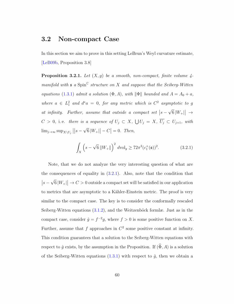
3.2 Non-compact Case

In this section we aim to prove in this setting LeBrun’s Weyl curvature estimate,

[LeB09b, Proposition 3.8]

Proposition 3.2.1. Let (X, g) be a smooth, non-compact, finite volume 4-

manifold with s a SpinC structure on X and suppose that the Seiberg-Witten

equations (1.3.1) admit a solution (Φ, A), with ‖Φ‖ bounded and A = A0 + a,

where a ∈ L21 and d∗a = 0, for any metric which is C2 asymptotic to g

at infinity. Further, assume that outside a compact set∣∣s−√6 |W+|

∣∣ →C > 0, i. e. there is a sequence of Uj ⊂ X,

⋃Uj = X, Uj ⊂ Uj+1, with

limj→∞ supX\Uj

∣∣∣∣s−√6 |W+|∣∣− C∣∣ = 0. Then,

∫X

(s−√

6 ‖W+‖)2

dvolg ≥ 72π2(c+1 (s))2. (3.2.1)

Note, that we do not analyze the very interesting question of what are

the consequences of equality in (3.2.1). Also, note that the condition that∣∣s−√6 |W+|∣∣→ C > 0 outside a compact set will be satisfied in our application

to metrics that are asymptotic to a Kahler-Einstein metric. The proof is very

similar to the compact case. The key is to consider the conformally rescaled

Seiberg-Witten equations (3.1.2), and the Weitzenbock formlæ. Just as in the

compact case, consider g = f−2g, where f > 0 is some positive function on X.

Further, assume that f approaches in C2 some positive constant at infinity.

This condition guarantees that a solution to the Seiberg-Witten equations with

respect to g exists, by the assumption in the Proposition. If (Φ, A) is a solution

of the Seiberg-Witten equations (1.3.1) with respect to g, then we obtain a

60

solution (Φ, A) to the rescaled Seiberg-Witten equations (3.1.2) with respect

to g.

Let us set ψ = (Φ⊗ Φ)0. Then the Weitzenbock formula (1.2.12) yields

∫X

(‖∇ψ‖2 + s ‖ψ‖2 + f ‖ψ‖3) dvolg ≤ 0

We also have the Weitzenbock formula for the Hodge Laplacian (1.2.14) which

yields ∫X

‖∇ψ‖2 dvolg ≥∫X

(−2

√2

3‖W+‖ −

s

3

)‖ψ‖2 dvolg.

These two inequalities added together yield

∫X

((2

3s− 2

√2

3‖W+‖

)‖ψ‖2 + f ‖ψ‖3

)dvolg ≤ 0.

To simplify notation, let φ = 32ψ, and then rewriting the above inequality we

get ∫X

(√6 ‖W+‖ − s

)f−2/3(f 2/3 ‖φ‖2) dvolg ≥

∫X

f ‖φ‖3 dvolg

Now let us apply the Holder inequality with p = 3/2 and q = 3 to obtain

(∫X

∣∣∣s−√6 ‖W+‖∣∣∣3 f−2 dvolg

)1/3(∫X

f ‖φ‖3 dvolg

)2/3

≥∫X

f ‖φ‖3 dvolg

and so ∫X

∣∣∣s−√6 ‖W+‖∣∣∣3 f−2 dvolg ≥

∫X

f ‖φ‖3 dvolg. (3.2.2)

61

The Holder inequality with the same p and q also tells us

(∫X

f 4 dvolg

)1/3(∫X

f ‖φ‖3 dvolg

)2/3

≥∫X

f 3 ‖φ‖2 dvolg. (3.2.3)

Combining (3.2.2) and (3.2.3)

(∫X

f 4 dvolg

)1/3(∫X

∣∣∣s−√6 ‖W+‖∣∣∣3 f−2 dvolg

)2/3

≥∫X

f 2 ‖φ‖2 dvolg.

(3.2.4)

Now we use the rescaled Seiberg-Witten equation (3.1.2), fφ = 3√

2F+A to get

∫X

f 2 ‖φ‖2 dvolg = 18

∫X

∣∣F+A

∣∣2 dvolg ≥ 18(2πc+1 (s))2 = 72π2(c+

1 (s))2,

where the inequality follows by Proposition 2.5.2.

(∫X

f 4 dvolg

)1/3(∫X

∣∣∣s−√6 ‖W+‖∣∣∣3 f−2 dvolg

)2/3

≥ 72π2(c+1 (s))2. (3.2.5)

Now we choose a sequence fj →√∣∣s−√6 ‖W+‖

∣∣ uniformly from above.

Since f 2j ≥

∣∣s−√6 ‖W+‖∣∣, we have

∫X

f 4j dvolg ≥

∫X

∣∣∣s−√6 ‖W+‖∣∣∣2 dvolg =

=

∫X

(f

4/3j

)·(∣∣∣s−√6 ‖W+‖

∣∣∣2 f−4/3j

)dvolg ≥

≥(∫

X

f 4j dvolg

)1/3(∫X

∣∣∣s−√6 ‖W+‖∣∣∣3 f−2

j dvolg

)2/3

where the last inequality follows by once again applying Holder inequality with

62

p = 3/2 and q = 3. The right hand side in the inequality above is the left hand

side in (3.2.5), so we can combine the last inequality with (3.2.5) to obtain

∫X

f 4j ≥ 72π2(c+

1 (s))2. (3.2.6)

Now, since f 4j →

∣∣s−√6 ‖W+‖∣∣2 uniformly on M , we obtain the desired

estimate: ∫X

(s−√

6 ‖W+‖)2

dvolg ≥ 72π2(c+1 (s))2.

Corollary 3.2.2. With (X, g), s as in Proposition 3.2.1, we have

1

4π2

∫X

(s2

24+ 2 |W+|2

)dvolg ≥

2

3

(c+

1 (s))2. (3.2.7)

Proof. Following [LeB01]

9

8

∫X

(s2 + 48 |W+|2

)dvolg =

9

8

(‖s‖2

L2 + 48 ‖W+‖2L2

)(using the L2 norm in R2) =

∥∥∥⟨1, 1/√

8⟩∥∥∥2 ∥∥∥⟨‖s‖L2 ,

√48 ‖W+‖L2

⟩∥∥∥2

(by Cauchy-Schwarz in R2) ≥(⟨

1, 1/√

8⟩·⟨‖s‖L2 ,

√48 ‖W+‖L2

⟩)2

=(‖s‖L2 +

√6 ‖W+‖L2

)2

≥∥∥∥s−√6 |W+|

∥∥∥2

L2

=

∫X

(s−√

6 |W+|)2

dvolg

≥ 72π2(c+

1 (s))2

(3.2.8)

and the inequality follows.

63

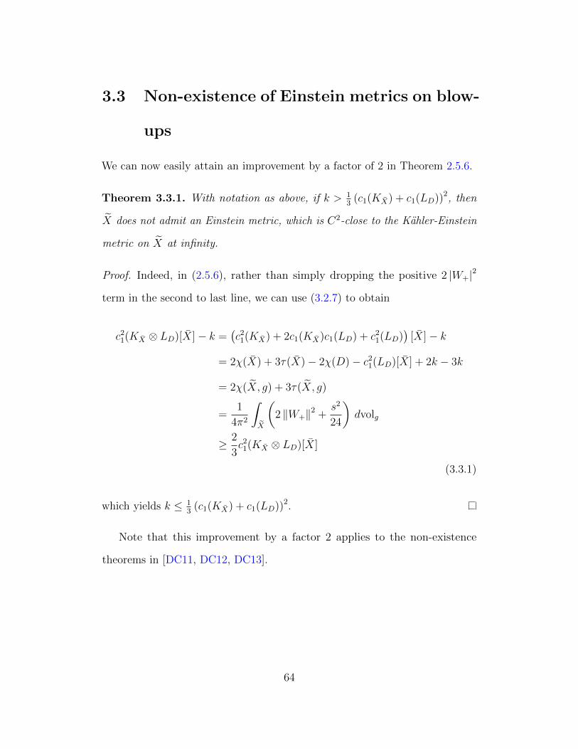
3.3 Non-existence of Einstein metrics on blow-

ups

We can now easily attain an improvement by a factor of 2 in Theorem 2.5.6.

Theorem 3.3.1. With notation as above, if k > 13

(c1(KX) + c1(LD))2, then

X does not admit an Einstein metric, which is C2-close to the Kahler-Einstein

metric on X at infinity.

Proof. Indeed, in (2.5.6), rather than simply dropping the positive 2 |W+|2

term in the second to last line, we can use (3.2.7) to obtain

c21(KX ⊗ LD)[X]− k =

(c2

1(KX) + 2c1(KX)c1(LD) + c21(LD)

)[X]− k

= 2χ(X) + 3τ(X)− 2χ(D)− c21(LD)[X] + 2k − 3k

= 2χ(X, g) + 3τ(X, g)

=1

4π2

∫X

(2 ‖W+‖2 +

s2

24

)dvolg

≥ 2

3c2

1(KX ⊗ LD)[X]

(3.3.1)

which yields k ≤ 13

(c1(KX) + c1(LD))2.

Note that this improvement by a factor 2 applies to the non-existence

theorems in [DC11, DC12, DC13].

64

Appendix A

Analysis

For a general introduction to Sobolev spaces see [Tay11a, Chapter 4], for the L2

theory and [Tay11c, Chapter 13] for the Lp theory. Another excellent reference

is [Eva10], or the Appendix to [DK90]. For the convenience of the reader

we quote the basic definitions of Sobolev spaces and the two basic theorems

regarding them.

Definition A.1. Lpk(Rn) =f ∈ Lp(Rn)

∣∣ ∂mi1,...,imf ∈ Lp(Rn), 0 ≤ m ≤ k

where the partial derivatives are understood in a weak sense. Naturally, the

Lpk-norm is defined as ‖f‖Lpk(Rn) =

∑|α|≤k

∥∥∥∂|α|α f∥∥∥Lp(Rn)

, where α = (i1, . . . , in),

|α| =∑il, is a multi-index. It is easy to see that C∞0 (Rn) is dense in Lpk(Rn),

hence, an a posteriori equivalent definition of Lpk(Rn) is the completion of

C∞0 (Rn) with respect to the Lpk-norm. Further, since multiplication by a com-

pactly supported smooth function sends Lpk(Rn) to itself, by using a partition

of unity, we can define Lpk(M) on a manifold.

Note that in the case p = 2, there is an equivalent definition of L2k using the

65

Fourier transform, ‖f‖L2k(Rn) =

∥∥∥(1 + t2)k/2f(t)∥∥∥L2(Rn)

, where f is the Fourier

transform of f .

Theorem A.2 (Sobolev Embedding). Suppose k > l and 1 ≤ p < q ≤ ∞ and

(k − l)p < n. Then Lpk(Rn) → Lql (Rn) for 1q

= 1p− k−l

nand the embedding is

compact if k > l and k − n/p > l − n/q.

Suppose k−r−αn

= 1p, then Lpk(Rn) → Cr,α(Rn). Where Cr,α(Rn) are the

usual Holder spaces.

The compactness statement is known as the Rellich-Kondrachov Theorem.

These statements also hold on a compact n-dimensional manifold, a compact

n-dimensional manifold with Lipschitz boundary, and a complete Riemannian

manifold with bounded sectional curvature and injectivity radius bounded

away from zero. Note the special cases we need, L21(X

4) → L4(X4) and

L22(X4) → C0(X4) for a compact 4-manifold X4.

Theorem A.3 (Sobolev Multiplication). Suppose 1/p − k/n > 0 and

1/q − l/n > 0 and 0 < m/n + (1/p − k/n) + (1/q − l/n) ≤ 1/r ≤ 1. Then

Lpk × Lql → Lrm. If k/n − 1/p > 0, k ≥ l and k/n − 1/p ≥ l/n − 1/q then

Lpk × Lql → Lql .

Note the particular case we need in dimension 4, L23 × L2

2 → L22 and l ≥ 3,

L2l × L2

l → L2l .

Theorem A.4 (Garding Inequality). Let E and F be two vector bundles over

some manifold X and suppose D : Γ(E) → Γ(F ) is an elliptic differential

operator of order l. Then for s ∈ Γ(E)

‖s‖L2k+l≤ C

(‖Ds‖L2

k+ ‖s‖L2

)66

Further, if s is orthogonal to the kernel of D, then

‖s‖L2k+l≤ C ‖Ds‖L2

k.

67

Bibliography

[AL13] Michael Atiyah and Claude Lebrun, Curvature, cones and character-istic numbers, Math. Proc. Cambridge Philos. Soc. 155 (2013), no. 1,13–37, URL: http://dx.doi.org/10.1017/S0305004113000169.

[And88] Michael T. Anderson, L2 harmonic forms on complete Rieman-nian manifolds, Geometry and analysis on manifolds (Katata/Kyoto,1987), Lecture Notes in Math., vol. 1339, Springer, Berlin, 1988,pp. 1–19, URL: http://dx.doi.org/10.1007/BFb0083043. 50

[Biq97] Olivier Biquard, Metriques d’Einstein a cusps et equations de Seiberg-Witten, J. Reine Angew. Math. 490 (1997), 129–154, URL: http://dx.doi.org/10.1515/crll.1997.490.129. iii, 36, 53

[Boc46] S. Bochner, Vector fields and Ricci curvature, Bull. Amer. Math. Soc.52 (1946), 776–797, URL: http://projecteuclid.org/download/pdf_1/euclid.bams/1183509635. 16

[Bou81a] Jean-Pierre Bourguignon, Formules de Weitzenbock en dimension4, Riemannian geometry in dimension 4 (Paris, 1978/1979), TextesMath., vol. 3, CEDIC, Paris, 1981, pp. 308–333. 14, 16

[Bou81b] , Les varietes de dimension 4 a signature non nulle dont lacourbure est harmonique sont d’Einstein, Invent. Math. 63 (1981),no. 2, 263–286, URL: http://dx.doi.org/10.1007/BF01393878.16

[Car23] Elie Cartan, Sur les varietes a connexion affine et la theorie de larelativite generalisee (premiere partie), Ann. Sci. Ecole Norm. Sup.(3) 40 (1923), 325–412, URL: http://www.numdam.org/item?id=ASENS_1923_3_40__325_0. 1

[Car02] Gilles Carron, L2 harmonic forms on non-compact Riemannian man-ifolds, Surveys in analysis and operator theory (Canberra, 2001),

68

Proc. Centre Math. Appl. Austral. Nat. Univ., vol. 40, Austral. Nat.Univ., Canberra, 2002, pp. 49–59. 50

[CY80] Shiu Yuen Cheng and Shing Tung Yau, On the existence of a completeKahler metric on noncompact complex manifolds and the regularityof Fefferman’s equation, Comm. Pure Appl. Math. 33 (1980), no. 4,507–544, URL: http://dx.doi.org/10.1002/cpa.3160330404. 29

[DC11] Luca Fabrizio Di Cerbo, Seiberg-Witten equations on certain man-ifolds with cusps, New York J. Math. 17 (2011), 491–512, URL:http://nyjm.albany.edu:8000/j/2011/17_491.html. iii, 36, 53,64

[DC12] , Finite-volume complex surfaces without cuspidal Einsteinmetrics, Ann. Global Anal. Geom. 41 (2012), no. 3, 371–380, URL:http://dx.doi.org/10.1007/s10455-011-9289-6. iii, 36, 53, 64

[DC13] , Seiberg-Witten equations on surfaces of logarithmic generaltype, Internat. J. Math. 24 (2013), no. 9, 1350074, 23, URL: http://dx.doi.org/10.1142/S0129167X13500742, arXiv:1112.0694. 64

[Dir28] Paul A.M. Dirac, The quantum theory of the electron, Proceedings ofthe Royal Society of London. Series A. 117 (1928), no. 778, 610–624.13

[DK90] S. K. Donaldson and P. B. Kronheimer, The geometry of four-manifolds, Oxford Mathematical Monographs, The Clarendon PressOxford University Press, New York, 1990, Oxford Science Publica-tions. 2, 22, 65

[Ehr51] Charles Ehresmann, Les connexions infinitesimales dans un espacefibre differentiable, Colloque de topologie (espaces fibres), Bruxelles,1950, Georges Thone, Liege, 1951, pp. 29–55. 1

[Ein16] Albert Einstein, Die grundlage der allgemeinen relativitatstheorie,Annalen der Physik 354 (1916), no. 7, 769–822. 1

[Eva10] Lawrence C. Evans, Partial differential equations, second ed., Gradu-ate Studies in Mathematics, vol. 19, American Mathematical Society,Providence, RI, 2010. 65

[FM97] Robert Friedman and John W. Morgan, Algebraic surfaces andSeiberg-Witten invariants, J. Algebraic Geom. 6 (1997), no. 3, 445–479, arXiv:alg-geom/9502026. 56

69

[Gue] Henri Guenancia, Khler-einstein metrics: from cones to cusps, Toappear. 45

[Hat] Allen Hatcher, Spectral sequences in algebraic topology,http://www.math.cornell.edu/ hatcher/SSAT/SSATpage.html. 5

[JO01] J. D. Jackson and L. B. Okun, Historical roots of gauge invariance,Rev. Mod. Phys. 73 (2001), 663–680. 1

[Jos11] Jurgen Jost, Riemannian geometry and geometric analysis, sixthed., Universitext, Springer, Heidelberg, 2011, URL: http://dx.doi.org/10.1007/978-3-642-21298-7. 21

[JPW96] Jurgen Jost, Xiaowei Peng, and Guofang Wang, Variational aspectsof the Seiberg-Witten functional, Calc. Var. Partial Differential Equa-tions 4 (1996), no. 3, 205–218, URL: http://dx.doi.org/10.1007/BF01254344, arXiv:dg-ga/9504003. 21

[KM94] P. B. Kronheimer and T. S. Mrowka, The genus of embedded surfacesin the projective plane, Math. Res. Lett. 1 (1994), no. 6, 797–808. 18

[KM07] , Floer homology for Seiberg-Witten Monopoles, CambridgeUniversity Press, 2007. 20, 23

[Kob84] Ryoichi Kobayashi, Kahler-Einstein metric on an open algebraicmanifold, Osaka J. Math. 21 (1984), no. 2, 399–418, URL: http://projecteuclid.org/getRecord?id=euclid.ojm/1200777118. 29,30

[Lab07] Mohammed Larbi Labbi, On weitzenbock curvature operators, arXiv:math/0607521. 14

[LeB95a] Claude LeBrun, Einstein metrics and Mostow rigidity, Math. Res.Lett. 2 (1995), no. 1, 1–8. iii, 53

[LeB95b] , Polarized 4-manifolds, extremal Kahler metrics, and Seiberg-Witten theory, Math. Res. Lett. 2 (1995), no. 5, 653–662, URL:http://dx.doi.org/10.4310/MRL.1995.v2.n5.a10.

[LeB96] , Four-manifolds without Einstein metrics, Math. Res. Lett.3 (1996), no. 2, 133–147, URL: http://dx.doi.org/10.4310/MRL.1996.v3.n2.a1. 56

70

[LeB98] , Weyl curvature, Einstein metrics, and Seiberg-Witten theory,Math. Res. Lett. 5 (1998), no. 4, 423–438, URL: http://dx.doi.org/10.4310/MRL.1998.v5.n4.a1. 56

[LeB01] , Ricci curvature, minimal volumes, and Seiberg-Witten theory,Invent. Math. 145 (2001), no. 2, 279–316, URL: http://dx.doi.org/10.1007/s002220100148. 56, 58, 63

[LeB02] , Hyperbolic manifolds, harmonic forms, and Seiberg-Witteninvariants, Proceedings of the Euroconference on Partial Differen-tial Equations and their Applications to Geometry and Physics(Castelvecchio Pascoli, 2000), vol. 91, 2002, pp. 137–154, URL:http://dx.doi.org/10.1023/A:1016222709901.

[LeB03] , Einstein metrics, four-manifolds, and differential topology,Surveys in differential geometry, Vol. VIII (Boston, MA, 2002), Surv.Differ. Geom., VIII, Int. Press, Somerville, MA, 2003, pp. 235–255,URL: http://dx.doi.org/10.4310/SDG.2003.v8.n1.a8.

[LeB09a] , Einstein metrics, four-manifolds, and conformally Kahlergeometry, Surveys in differential geometry. Vol. XIII. Geometry, anal-ysis, and algebraic geometry: forty years of the Journal of DifferentialGeometry, Surv. Differ. Geom., vol. 13, Int. Press, Somerville, MA,2009, pp. 135–147, URL: http://dx.doi.org/10.4310/SDG.2008.v13.n1.a5.

[LeB09b] , Four-manifolds, curvature bounds, and convex geometry,Riemannian topology and geometric structures on manifolds, Progr.Math., vol. 271, Birkhauser Boston, Boston, MA, 2009, pp. 119–152,URL: http://dx.doi.org/10.1007/978-0-8176-4743-8_6. 58, 60

[LeB12] , On Einstein, Hermitian 4-manifolds, J. Differential Geom.90 (2012), no. 2, 277–302, URL: http://projecteuclid.org/

getRecord?id=euclid.jdg/1335230848.

[LeB13a] Claude LeBrun, Edges, orbifolds, and seiberg-witten theory, arXiv:1305.1960. 41, 42, 43, 44

[LeB13b] Claude LeBrun, Einstein manifolds and extremal Kahler metrics, J.Reine Angew. Math. 678 (2013), 69–94.

[Lic63] Andre Lichnerowicz, Spineurs harmoniques, C. R. Acad. Sci. Paris257 (1963), 7–9. 15

71

[LM89] H. Blaine Lawson, Jr. and Marie-Louise Michelsohn, Spin geometry,Princeton Mathematical Series, vol. 38, Princeton University Press,Princeton, NJ, 1989. 3, 14

[Max65] James Clerk Maxwell, A dynamical theory of the electromagneticfield, Philosophical Transactions of the Royal Society of London 155(1865), 459–512. 1

[Moo01] John Douglas Moore, Lectures on Seiberg-Witten invariants, seconded., Lecture Notes in Mathematics, vol. 1629, Springer-Verlag, Berlin,2001. 18

[Mor96] John W. Morgan, The Seiberg-Witten equations and applications tothe topology of smooth four-manifolds, Mathematical Notes, vol. 44,Princeton University Press, Princeton, NJ, 1996. 3, 12, 18, 23, 28

[Nic00] Liviu I. Nicolaescu, Notes on Seiberg-Witten theory, Graduate Studiesin Mathematics, vol. 28, American Mathematical Society, Providence,RI, 2000, URL: http://www3.nd.edu/~lnicolae/swnotes.pdf. 18,56

[Pet] Peter Petersen, Demystifying the weitzenbck curvature operator, URL:http://www.math.ucla.edu/~petersen/BLWformulas.pdf. 14

[Roe98] John Roe, Elliptic operators, topology and asymptotic methods, sec-ond ed., Pitman Research Notes in Mathematics Series, vol. 395,Longman, Harlow, 1998. 14, 15

[Roh52] V. A. Rohlin, New results in the theory of four-dimensional manifolds,Doklady Akad. Nauk SSSR (N.S.) 84 (1952), 221–224. 7

[Rol02] Yann Rollin, Surfaces kahleriennes de volume fini et equations deSeiberg-Witten, Bull. Soc. Math. France 130 (2002), 409–456. 36, 53

[Rol04] , Rigidite d’Einstein du plan hyperbolique complexe, J. ReineAngew. Math. 567 (2004), 175–213, URL: http://dx.doi.org/10.1515/crll.2004.010. iii

[Sal99] Dietmar Salamon, Spin geometry and seiberg-Witten invariants,1999, URL: http://www.math.ethz.ch/~salamon/PREPRINTS/

witsei.pdf. 18

[Sch98] Georg Schumacher, Asymptotics of Kahler-Einstein metrics on quasi-projective manifolds and an extension theorem on holomorphic maps,

72

Math. Ann. 311 (1998), no. 4, 631–645, URL: http://dx.doi.org/10.1007/s002080050203. 33

[Sch02] , Asymptotics of complete Kahler-Einstein metrics—negativityof the holomorphic sectional curvature, Doc. Math. 7 (2002), 653–658(electronic). 33

[SW94] Nathan Seiberg and Edward Witten, Electric-magnetic duality,monopole condensation, and confinement in N = 2 supersymmet-ric Yang-Mills theory, Nuclear Physics B 426 (1994), no. 1, 19–52,arXiv:hep-th/9407087. 17

[Tay11a] Michael E. Taylor, Partial differential equations I. Basic theory, sec-ond ed., Applied Mathematical Sciences, vol. 115, Springer, New York,2011, URL: http://dx.doi.org/10.1007/978-1-4419-7055-8. 65

[Tay11b] , Partial differential equations II. Qualitative studies of lin-ear equations, second ed., Applied Mathematical Sciences, vol. 116,Springer, New York, 2011, URL: http://dx.doi.org/10.1007/

978-1-4419-7052-7. 2, 14, 15

[Tay11c] , Partial differential equations III. Nonlinear equations, seconded., Applied Mathematical Sciences, vol. 117, Springer, New York,2011, URL: http://dx.doi.org/10.1007/978-1-4419-7049-7. 3,65

[TY87] G. Tian and S.-T. Yau, Existence of Kahler-Einstein metrics on com-plete Kahler manifolds and their applications to algebraic geometry,Mathematical aspects of string theory (San Diego, Calif., 1986), Adv.Ser. Math. Phys., vol. 1, World Sci. Publishing, Singapore, 1987,pp. 574–628. 29

[Wey29] Hermann Weyl, Elektron und gravitation. i, Zeitschrift fur Physik AHadrons and Nuclei 56 (1929), no. 5, 330–352. 1

[Wit94] Edward Witten, Monopoles and four-manifolds, Math. Res. Lett. 1(1994), no. 6, 769–796. 17, 28

[YM54] Chen-Ning Yang and Robert L Mills, Conservation of isotopic spinand isotopic gauge invariance, Physical review 96 (1954), no. 1, 191.1

73