water resistivity for western latvia ordovician … resistivity for western latvia ordovician zone...

Water Resistivity for Western Latvia Ordovician Zone Otis P. Armstrong, P.E.

1

Abstract: These considerations are given because of uncertainties in Soviet era well logs. Specifically, a lack of water analysis from which Ordovician water resistivity values could be determined. Water Resistivity is an important factor used to calculate porosity and water saturation. Water samples were available for Cambium age, Figure 1, and lower Devonian age, ( 4 to 8 g/l) but missing for Ordovician and Silurian age rocks. A lack of free flowing Ordovician water, was reported to prevented sampling and analysis. Also, the self potential, SP, data were reported to be less than analytical quality. Compounding the problems of SP data were a lack of mud filtrate resistivity values and uncertainty in chart factors. However, a major shift in SP and deep resistivity, RL, appeared across the Ordovician and Cambrium boundary, in most well logs; while the Normal resistivity Sonde value, RN, remained fairly constant. Also, when making Pickett type plots of Neutron-Gamma Ray deflection vs. log of deep resistivity, there was an improvement in “goodness of fit, R2” for the baseline “Sw = 1”, if separate plots were made for Ordovician and Cambrium sections. Plus the calculated Pickett values of Rw for Ordovician averaged higher than Rw of Cambrium sections. But, a simple analysis of core porosity contradicted the values obtained from the Pickett Plots, SP and sectional resistivity data. This contradiction was resolved by using shale analysis. Details of his novel method are provided in the appendix. In summary, a water resistivity of 0.13 o-m at 68F, 20C, or 56,000 ppm, NaCl Eqiv., is proposed for Ordovician water in this area. This compares to approximately 120g/l or 120,000 ppm for the mid Cambrium section .. Also, this paper presents a method to ascertain the effect of shale in a formation on resistivity derived water saturation values. This was done by introduction of a shale factor, Fs, into Archie’s water saturation equation. The Archie equation is revised to read: Sw =√(FsFRw/Rt) Fs = {5C2}/[1 + 2C(FRw/Sw)*(V/R)s ] Sxo = √(Fs-xoFRmf/Rxo) Fs-xo = {5C2}/[1 + 2C(FRmf/Sxo)*(V/R)s ]

With these equations water saturation can be rapidly interpolated either directly or with aid from a Picket plot, as detailed in the appendix. The primary use here is for plotting effect of shale in Pickett chart.


2

Abstract: 1.1 Overview 1.2 Cambrium Water Mineralization 1.3 Resistivity Ratio between Cambrium and Ordovician Sections 1.4 Ordovician Water Mineralization by SP ratio 1.5 Ordovician Water Mineralization by Pickett Plot 1.6 Ordovician Water by Shale Parameters 1.7 Summary Figure 1. H2O Resistivity by Mineralization @ 75F Mid-west Latvia Cambrium Figure. 2 Determination of Ordovician Rw by SP Data Figure 3 Effect of Rw on need for Shale Analysis Comparison of Wylie Data to Simandoux Equation Figure 4 Effect of Rw on need for Shale Analysis at Large F (low porosity) Comparison by Simandoux Equation Figure 5 Effect of Sw on I =R”@Sw/R”@Sw=1 Comparison of Wylie Data at F = 5 & by Simandoux Equation for F=5 & for F = 125, low porosity Figure 6 Low Open Porosity Effect on Rt for Sw = 50% and 100% at Moderate Shale% Figure 7 Plot of Long Electrical Survey Tool, RL to Determine Rs and RwNormal Electrical Survey Figure 8 Plot of Normal Electrical Survey Tool, Rn to Determine Rs and Rmf Figure 9 Well K15 Pickett Plot for RL with Shale Correction Points Ordv Section Figure 10 Well K15 Pickett Plot for Rn with Shale Correction Points Ordv. Section APPENDIX Appendix Background Appendix Summary A.I.1: Derivation of F sub shale, Fs, Equation from Simandoux Equation A.I.2: Determination of Rs & Rw When F is Known A.I.3. Determination of F from Shale Factors when Rw & Rs are known A.I.4 Sectional Summary APPENDIX II A.II.1 Conductivity Equation Review AII.2 Comparisons of Wylie Core Data to Simandoux Equations A.II.3 Formation Resistance For Picket Plots A.II.4 RESISTIVITY RATIO WITH SHALE CONSIDRATIONS A.II.5 RESISTIVITY INDEX WITH SHALE CONSIDRATIONS A.II.6 PICKETT PLOTS APPENDIX III Discussion of Porosity Factors


3

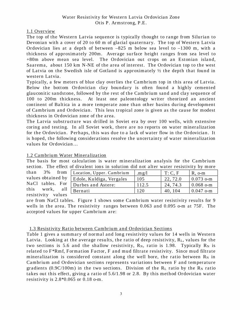
1.1 Overview The top of the Western Latvia sequence is typically thought to range from Silurian to Devonian with a cover of 20 to 60 m of glacial quaternary. The top of Western Latvia Ordovician lies at a depth of between –825 m below sea level to –1300 m, with a thickness of approximately 200m. Average surface height ranges from sea level to +80m above mean sea level. The Ordovician out crops on an Estonian island, Saarema, about 150 km N-NE of the area of interest. The Ordovician top to the west of Latvia on the Swedish isle of Gotland is approximately ½ the depth that found in western Latvia. Typically, a few meters of blue clay overlies the Cambrium top in this area of Latvia. Below the bottom Ordovician clay boundary is often found a highly cemented glauconitic sandstone, followed by the rest of the Cambrium sand and clay sequence of 100 to 200m thickness. At least one paleontology writer theorized an ancient continent of Baltica in a more temperate zone than other basins during development of Cambrium and Ordovician. This less tropical zone is given as the cause for modest thickness in Ordovician zone of the area. The Latvia substructure was drilled in Soviet era by over 100 wells, with extensive coring and testing. In all Soviet work, there are no reports on water mineralization for the Ordovician. Perhaps, this was due to a lack of water flow in the Ordovician. It is hoped, the following considerations resolve the uncertainty of water mineralization values for Ordovician… 1.2 Cambrium Water Mineralization The basis for most calculation is water mineralization analysis for the Cambrium section. The effect of divalent ions in solution did not alter water resistivity by more than 3% from values obtained by NaCl tables. For this work, all resistivity values are from NaCl tables. Figure 1 shows some Cambrium water resistivity results for 9 wells in the area. The resistivity ranges between 0.063 and 0.095 o-m at 75F. The accepted values for upper Cambrium are:

1.3 Resistivity Ratio between Cambrium and Ordovician Sections Table 1 gives a summary of normal and long resistivity values for 14 wells in Western Latvia. Looking at the average results, the ratio of deep resistivity, RL, values for the two sections is 5.6 and the shallow resistivity, RN, ratio is 1.98. Typically RN is related to F*Rmf, Formation Factor, F and mud filtrate resistivity. Since mud filtrate mineralization is considered constant along the well bore, the ratio between RN in Cambrium and Ordovician sections represents variations between F and temperature gradients (0.9C/100m) in the two sections. Division of the RL ratio by the RN ratio takes out this effect, giving a ratio of 5.6/1.98 or 2.8. By this method Ordovician water resistivity is 2.8*0.065 or 0.18 o-m.

Location, Upper. Cambrium .mg/l T: C, F R, o-m Edole, Kuldiga, Vergales 105 22, 72.0 0.073 o-m Durbes and Astere: 112.5 24, 74.3 0.068 o-m Bernati 120 40, 104 0.047 o-m


4

The same result would be obtained if RL ratio were compared between sections for which RN in Cambrium and Ordovician horizons were equal. In which case the ratio between RL for these two sections would be the ratio between water mineralization in Cambrium and Ordovician sections of equal porosity.

Table 1 Average Section Resistivity The ratio of RN/RL, for a given section, typically eliminates formation factors, and the result should be Rmf/Rw. Since Rmf should be the same along the borehole, taking the ratio of Rmf/Rw for Ordovician and Cambrium can give a pseudo water resistivity ratio, which for the below table comes to 2.7, indicating Rw Ordovician of 0.18o-m at an average Cambrium water R of 0.065. When shale and temperature factors are applied, Eqn.A-25, Ordovician water calculates to be 0.14 o-m, see appendix for details. Rw/Rmf = (Rt/Rxo) *[1 + 2C(FRw)*(V/R)s ]/[1 + 2C(FRmf)*(V/R)s ] A25 1.4 Ordovician Water Mineralization by SP ratio The Cambrium in the area of interest, is mostly medium porosity sandstone with intermixed shale, while Ordovician is mostly low porosity carbonates, shale or mixtures. In the case of resistivity, this shift could be influenced by porosity, lithology or changes in both. However, SP data in a thick, HC free bed, is responsive only to changes in shale volume content. So the difference in maximum SP deflections between two clean, thick beds can be related to Ordovician Rw as follows: (-SP/K) = (log Rmf/Rw) = (logRmf – logRw) Eq1 Since the thermal gradient is low and less than 200m between sections, an average K could be assumed effective and Rmf should also be about the same in the two sections. (if SP deflection is not fully developed, flat lined, then bed thickness correction should be applied; SP = SPdef*CFz , where CFz is always greater than or equal to 1.00) CFz = exp[1.245(ln(Ri/Rm))/z’-0.591/z’-0.133], z=bed thickness, ft Eq.1a Comparison of maximum SP’s between Ordovician and Cambrium gives the following simplistic equation for Rw in Ordovician:

Ord Ord Ord Camb Camb Camb

well RL RN Rn/RL RL RN Rn/RL

V50 5.0 20.0 4.0 1.0 6.0 6.0 KAz6d 20.0 15.0 0.8 0.7 5.0 7.1 K5 4.0 3.5 0.9 0.9 7.0 7.8 K4 4.0 4.0 1.0 1.5 5.0 3.3 K3 4.0 4.0 1.0 1.0 5.0 5.0 K13 13.0 70.0 5.4 7.0 20.0 2.9 Ed60 10.0 10.0 1.0 0.9 5.0 5.6 Ed17 14.0 12.0 0.9 1.0 7.0 7.0 D35 8.0 7.0 0.9 3.0 5.0 1.7 D15 16.0 11.0 0.7 1.2 6.0 5.0 D14 16.0 14.0 0.9 1.5 7.0 4.7 D13 5.0 3.0 0.6 0.6 4.0 6.7 B6 15.0 4.0 0.3 2.0 4.0 2.0 B20 8.0 8.0 1.0 3.0 8.0 2.7 avg 10.1 13.3 1.4 1.8 6.7 4.8


5

(Rw)ordv. = alog(log(Rw).cmb +[(SP).ord – (SP).cmb]/K + C) Eq. 2

The chart factor, C, is the offset factor which makes (–SP/K) equal to zero when Rw equals Rmf. Results of this analysis for Cambrium Rw = 0.065 is given in Figure 2, below: The statistical average for this method is 0.21, the result for well K13 was discarded, being 3 times greater than the average. 1.5 Ordovician Water Mineralization by Pickett Plot When the Pickett method was applied to Ordovician section of 7 well logs, 0.13 was the average Rw, with a range of 0.09 to 0.18 o-m. This method made an educated assumption about the porosity range. The Cambrium section average for 4 wells was 0.049 o-m. The method details are given by the Appendix. Briefly it is as follows :use Eq.A35a or b to calculate porosity for F=10, then apply A38 to get ND, and lastly, apply 40a,b to arrive at Rw or Rmf. 1.6 Ordovician Water by Shale Parameters The Appendix proposes to calculate Rw using shale parameters, those results arrive at an Ordovician water salinity of 0.121 o-m at 68F, 0.091 o-m at 93F. This method does not rely on Cambrium water analysis. In this instance, core porosity was used to determine F and plots the product of F and shale volume, Vs, against the ratio F over log resistivity, Eq.A16. The slope and intercept of the regression line provide values of Shale resistivity and aqueous phase resistivity. Figures 6 and 7 plus the below tables of Normal and Long survey tools were taken for well Bernati 2, Ordovician zone using core open porosity. The result for RL is given in Table 2 and Figure 6.

Table 2: B2 Plot Results, RL, The average Ordovician water resistivity calculated by shale equations (column B) is about 0.09, at 40C. This compares to 0.05 (E) when determined by Archie Equation with open porosity, which ignored shale effects.

F= 1/φ2 carbs 0.81/φ2 consol sands A35 Log(φ, v/v) = U – V*ND A38 At F =10 Rw = Rt/10 Rmf = Rxo/10 A40a, b

F/Rt = FVs 2/(5CRs) + 1/(Rw5C2) Eq.A16a

F/Rn = FVs 2/(5CRs) + 1/({Rmf}5C2) Eq.A16b

Rw Rs r2 Rw=RL/Fa Rw=RL/FeRL 0.099 1.61 0.38 Shale eqn Regr plot RL avg 0.091 1.75 na 0.052 0.061 A B C D E F


6

When porosity is increased by (1+Vs), Rw calculates higher, 0.06, (F) when ignoring shale effect, Fs=1. Shale resistivity, is determined from regression equation intercept, Eqn. 14 a & b. However, since shale conductivity theory implies Rs is independent of saturating water solution, then Rs is averaged between the values obtained in Figures 6 & 7 for Rn and RL, results in bottom row of Tables 2&3. Using the average of shale resistivity for Normal and Long Sonde gives an average Rw and Rmf (mud filtrate), bottom row, Tables 2 & 3. Shale resistivity value, Rs, for Ordovician of well B2, when corrected for temperature to 68F is 2.3 o-m. This value is very close to the statistical value of 2.8 for the wells listed in Table 4. The water resistivity value Rw for Ordovician of well B2, when corrected for temperature to 68F is 0.12 o-m. This value is close to the statistical average value of 0.17 for the wells listed in Table 4, and much higher than Cambrium water resistivity. Table 3: B2 Plot Results, Rn

Table 3 provides the results for the same calculations for the normal survey sonde. The normal sonde has

a shorter spacing and investigation depth. The log data did not provide details about mud filtrate resistivity. Mud gravity’s were reported to range between 1.1 and 1.28.

Table 4 gives the values of Rs and Rw determined from 11 well logs of western

Latvia wells. These value were taken by regression using plot of F/R vs F/Vs per Eqn A16a/b. Porosity was from NGR by maximum and minimum porosity, Eqn A38. This method, by default, determines an average shale resistivity.

Table 4 Cambium. & Ordovician Rw & Rs results from Shale Plots

1.7. Summary By most methods, (resistivity ratio, with (2) and without shale factors (2b); SP ratio method (3); Pickett Plot, (PP, 4) and Rw by Shale plots (5&5c), the Ordovician water resistivity was calculated to be considerably more than 0.065o-m for Cambrium age.

Rmf Rs .r2 Rmf=Rn/Fo Rmf=Rn/Fe Rn 0.17 1.87 0.55 Rn avg 0.203 1.75 na 0.071 0.085

Well Cmb Rw Cmb Rs rr Ord Rw Ord Rs rr Ed17op 0.03 0.5 .1 0.21 3.1 .5 B2op 0.06 7.6 .5 0.166 2.46 .77 K13op 0.033 0.76 .54 0.28 1.4 .27 K15op 0.14 3.2 .1 K5op 0.063 0.56 0.03 0.195 4.1 0.82 KD6op 0.024 1.65 0.002 0.13 5.3 0.99 Ed60op 0.03 2.14 0.99 0.159 3.1 0.97 B20op 0.057 7.8 0.999 0.135 2.3 0.91 B24op 0.03 3.2 0.99 0.49 1.7 0.94 AP1op Na Na Na 0.12 2.1 0.83 AP2op Na Na Na 0.18 2.1 0.91 St. Avg 0.041 3.0 0.52 0.17 2.81 0.73


7

R-ratio R-r w/shale SP PP SF core B2 Core B2w/o SF SF avg Avg. All

2 2b 3 4 5 5b 5c #6

Rw Rw Rw Rw-o Rw-Ov= 20C Rw-o @40C Rw- Rw-o

0.18 0.14 0.21 0.13 0.12 0.065 0.17 0.146 The general average of water resistivity comes to 0.146 for all methods, column 6. The method involving the least amount of assumptions is shale factor plot (5) of porosity data. The shale factor, without core method, (5c) assumes a porosity range to determine F. The SP method (3) required an assumption of mud filtrate resistivity to arrive at the offset factor, C. This assumption of mud filtrate resistivity is marginal, given mud density, log resistivity in large caliber zones, and drilling practice, but nevertheless an assumption. The resistivity ratio method (2) neglects shale factor corrections. The appendix shows that shale corrections are more significant at low porosity or high resistivity. When shale factors are considered, Rw calculates lower (2b). The PP, method (4) assumes a porosity range. This “porosity range” is based on core analysis porosity ranges and the general rule that consolidated rock porosity seldom exceeds 28% and the physical principle that residual porosity is found in all but pure minerals. Shale factors and core porosity values indicate only a remote possibility of pure minerals, thus the porosity range of 6% to 28% for PP analysis. The recommended value is an average of methods, 2b, 4, and 5; which equals 0.13o-m at 20C.


8


9

H2O resist, o-m@75F, Camb & Lower;

Depth, m where available

estimated from H20 mineral analysis

1331

1325

1370

1230

1207

997

969

1055

1055

1023

1128

1128

1023 1055

0.0600.0650.0700.0750.0800.0850.0900.0950.100

v46

v46

v49

v49

v47

v47

v49

k14

kp5

kp11 v4

7

v50

v48

v65

v50

v50

v65

v48

Fig 2

Determination of Ordovician Rw by SP Data

0.00

0.10

0.20

0.30

0.40

0.50

0.60

0.70

k13 b20 d35 ed17 d15 k-11 ed60 d14 st. Avg

Rw

Ord

v

Figure 1 H2O Resistivity by Mineralization @ 75F Mid-west Latvia Cambrium


10

Figure 3 Effect of Rw on need for Shale Analysis

Comparison of Wylie Data to Simandoux Equation

1

10

0.1 1 10

RwSqrt(

Fa/F

o) F

a= ~

5

B-data A data S-Pred-B S-pred A

Figure 4

Effect of Rw on need for Shale Analysis at Large F (low porosity) Comparison by Simandoux Equation

1

1.2

1.4

1.6

1.8

2

2.2

2.4

25 75 125 175 225 275

F archie

SQR

T(F/

Fo)

Rw=0.13 (V/R)s=.125 Rw=0.07 V/R=.125

Rw=0.13 V/R=.023 Rw=0.07 V/R=.023


11

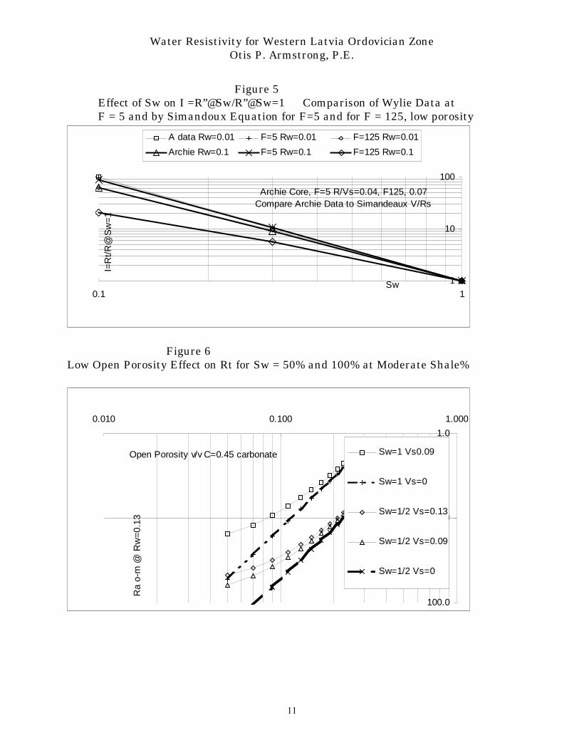
Figure 5

Effect of Sw on I =R”@Sw/R”@Sw=1 Comparison of Wylie Data at F = 5 and by Simandoux Equation for F=5 and for F = 125, low porosity

Archie Core, F=5 R/Vs=0.04, F125, 0.07Compare Archie Data to Simandeaux V/Rs

1

10

100

0.1 1Sw

I=R

t/R@

Sw=1

A data Rw=0.01 F=5 Rw=0.01 F=125 Rw=0.01Archie Rw=0.1 F=5 Rw=0.1 F=125 Rw=0.1

Figure 6 Low Open Porosity Effect on Rt for Sw = 50% and 100% at Moderate Shale%

1.0

10.0

100.0

0.010 0.100 1.000

Open Porosity v/v C=0.45 carbonate

Ra

o-m

@ R

w=0

.13

Sw=1 Vs0.09

Sw=1 Vs=0

Sw=1/2 Vs=0.13

Sw=1/2 Vs=0.09

Sw=1/2 Vs=0


12

Figure 7 Plot of Long Electrical Survey Tool, RL to Determine Rs and Rw

B2 Core Data

0

10

20

30

40

0 10 20 30FVs

F/R

L

Normal Electrical Survey Figure 8

Plot of Normal Electrical Survey Tool, Rn to Determine Rs and Rmf

core data

d, m

996.5

999.5

1006

.0 1068

.2

1086

.010

99.2

1126

.2

0

10

20

30

40

0 10 20 30FVs

F/R

n


13

Figure 9

Well K15 Pickett Plot for RL with Shale Correction Points Ordv Section

R15RL temp corr'd

986

984

980

975

970

965

962960955

950

945940

933

930 925920915

910 906

904

901897

895

892 890886885

881

876

870869

865862860

857

855853

850845842

841840

835

834

830

825820

1.0

10.0

100.0

5 15 25 35 45 55 65

ND, NGR

o-m

SL SL@Sw=1 Sw=0.5 Expon. (SL@Sw=1) Expon. (Sw=0.5)


14

Figure 10

Well K15 Pickett Plot for Rn with Shale Correction Points Ordv. Section

R15Rn temp corr'd

986

984

980

975

970

965

962

960

955

950

945940

933

930925

920915

910

906

904901

897

895892

890

886

885881

876

870869 865

862

860

857

855

853

850845842

841

840

835

834

830

825

820

1.0

10.0

100.0

5 15 25 35 45 55 65

ND, NGR

o-m

Sn Sn@Sw=1 Sw=0.5 Expon. (Sn@Sw=1) Expon. (Sw=0.5)


15

APPENDIX

Appendix Background Application of shale conductivity equations, permitted resolution of a substantial contradiction in water mineralization calculated from core open porosity, and particular attention is presented about this shale method. A good amount of technical literature presents rules for when to not use shale conductivity analysis, perhaps due to complications arising in the basic analysis equations. In the course of review, it seems that that no-one-single-factor is presented to represent the degree of shale effect on conductivity in porous media. This discussion presents a simplified approach using a new variant to the classic Archie conductivity equation, (Sw )2= F*Rw/Rt, namely, adding F sub shale, Fs. (Sw )2= Fo*Fs*Rw/Rt, Fs = {5C2}/[1 + 2C(FoRw/Sw)(V/R)s ] Eqn. A13 S2w-xo=Fo*Fsxo*Rmf/Rxo Fs-xo = {5C2}/[1 + 2C(FoRmf/Sxo)(V/R)s ] Eqn. A14

This single factor is valuable because it allows a rapid estimation of the degree to which shale conductivity pathway affects water saturation values. As Fs approaches one, effects of shale conductivity are reduced on overall conductivity. Also, presented is a method to predict simultaneously, shale and water resistivity for Laterolog. Prediction of shale resistivity is a noted weakness in application of shale analysis, Ref.1. What the Fs term does is to compensate for the increased calculated-resistivity from reduction of total porosity by the shale volume. Shale Analysis increases F by using open porosity, which is, total porosity, reduced by shale volume. For example, a shale section gives a large NGR porosity, although the open porosity is very low. Without the Fs term, the classic Archie equation using open porosity would calculate Rt as an erroneous large number. Appendix Summary Modification of the classic Archie conductivity equation by Fs introduces a new canon of analytical equations. Wylie (p57) initially proposed a similar concept for analysis of shaly sections with SP data by “apparent water resistivity”. Application of Fs introduces two new “apparent conductive fluids” namely, “apparent water” and “apparent mud filtrate” Rw-a = Rw*Fs, & Rmf-a = Rmf*Fs-xo, Eqn A13 & 14, When either Fs or the ratio Fs/Fs-xo deviate significantly from unity, then analytical equations need to use the “apparent water resistivity”, Rw-a and/or the “apparent mud filtrate resistivity” These analytical equations are variants of the two term shale conductivity equation, Simandoux modification of Wylie’s three term shale


16

conductivity equation. The restrictions for dropping this third term should be carefully reviewed, together with the validity of the shale terms. The following two term conductivity equation allows a fast evaluation with the basic constraint that L.H.S. term must be greater than or equal to zero:

{5C2/(Rt) – (2CSw)(V/R)s} = (Sw )2/(FRw) & is > or =0 A14b

{5C2/(Rxo) – (2CSwxo)(V/R)s} = (Swxo )2/(FRmf) & is > or =0 A14c

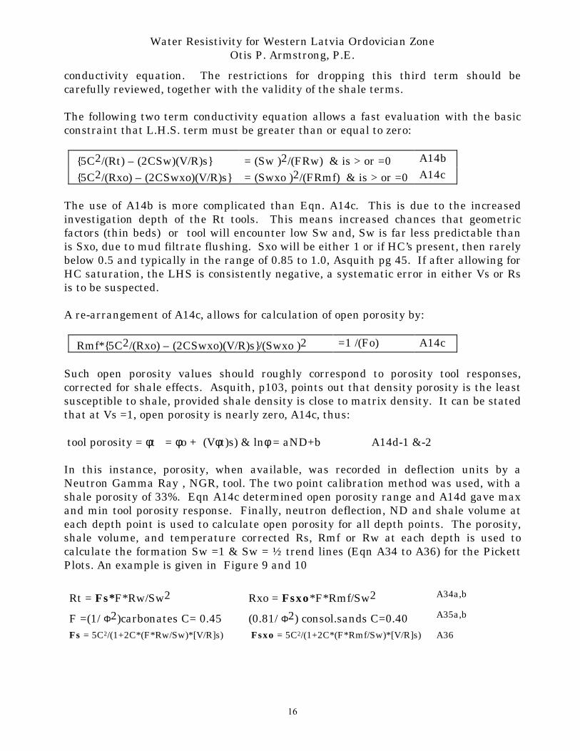
The use of A14b is more complicated than Eqn. A14c. This is due to the increased investigation depth of the Rt tools. This means increased chances that geometric factors (thin beds) or tool will encounter low Sw and, Sw is far less predictable than is Sxo, due to mud filtrate flushing. Sxo will be either 1 or if HC’s present, then rarely below 0.5 and typically in the range of 0.85 to 1.0, Asquith pg 45. If after allowing for HC saturation, the LHS is consistently negative, a systematic error in either Vs or Rs is to be suspected. A re-arrangement of A14c, allows for calculation of open porosity by:

Rmf*{5C2/(Rxo) – (2CSwxo)(V/R)s}/(Swxo )2 =1 /(Fo) A14c

Such open porosity values should roughly correspond to porosity tool responses, corrected for shale effects. Asquith, p103, points out that density porosity is the least susceptible to shale, provided shale density is close to matrix density. It can be stated that at Vs =1, open porosity is nearly zero, A14c, thus: tool porosity = φt = φo + (Vφt)s) & lnφ = aND+b A14d-1 &-2 In this instance, porosity, when available, was recorded in deflection units by a Neutron Gamma Ray , NGR, tool. The two point calibration method was used, with a shale porosity of 33%. Eqn A14c determined open porosity range and A14d gave max and min tool porosity response. Finally, neutron deflection, ND and shale volume at each depth point is used to calculate open porosity for all depth points. The porosity, shale volume, and temperature corrected Rs, Rmf or Rw at each depth is used to calculate the formation Sw =1 & Sw = ½ trend lines (Eqn A34 to A36) for the Pickett Plots. An example is given in Figure 9 and 10

Rt = Fs*F*Rw/Sw2 Rxo = Fsxo*F*Rmf/Sw2 A34a,b

F =(1/ Φ2)carbonates C= 0.45 (0.81/ Φ2) consol.sands C=0.40 A35a,b

Fs = 5C2/(1+2C*(F*Rw/Sw)*[V/R]s) Fsxo = 5C2/(1+2C*(F*Rmf/Sw)*[V/R]s) A36


17

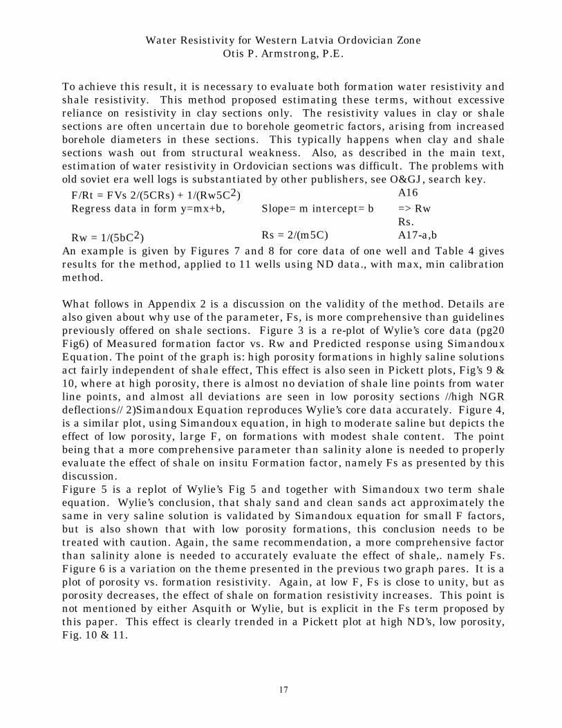
To achieve this result, it is necessary to evaluate both formation water resistivity and shale resistivity. This method proposed estimating these terms, without excessive reliance on resistivity in clay sections only. The resistivity values in clay or shale sections are often uncertain due to borehole geometric factors, arising from increased borehole diameters in these sections. This typically happens when clay and shale sections wash out from structural weakness. Also, as described in the main text, estimation of water resistivity in Ordovician sections was difficult. The problems with old soviet era well logs is substantiated by other publishers, see O&GJ, search key.

F/Rt = FVs 2/(5CRs) + 1/(Rw5C2) A16 Regress data in form y=mx+b, Slope= m intercept= b => Rw

Rs. Rw = 1/(5bC2) Rs = 2/(m5C) A17-a,b

An example is given by Figures 7 and 8 for core data of one well and Table 4 gives results for the method, applied to 11 wells using ND data., with max, min calibration method. What follows in Appendix 2 is a discussion on the validity of the method. Details are also given about why use of the parameter, Fs, is more comprehensive than guidelines previously offered on shale sections. Figure 3 is a re-plot of Wylie’s core data (pg20 Fig6) of Measured formation factor vs. Rw and Predicted response using Simandoux Equation. The point of the graph is: high porosity formations in highly saline solutions act fairly independent of shale effect, This effect is also seen in Pickett plots, Fig’s 9 & 10, where at high porosity, there is almost no deviation of shale line points from water line points, and almost all deviations are seen in low porosity sections //high NGR deflections// 2)Simandoux Equation reproduces Wylie’s core data accurately. Figure 4, is a similar plot, using Simandoux equation, in high to moderate saline but depicts the effect of low porosity, large F, on formations with modest shale content. The point being that a more comprehensive parameter than salinity alone is needed to properly evaluate the effect of shale on insitu Formation factor, namely Fs as presented by this discussion. Figure 5 is a replot of Wylie’s Fig 5 and together with Simandoux two term shale equation. Wylie’s conclusion, that shaly sand and clean sands act approximately the same in very saline solution is validated by Simandoux equation for small F factors, but is also shown that with low porosity formations, this conclusion needs to be treated with caution. Again, the same recommendation, a more comprehensive factor than salinity alone is needed to accurately evaluate the effect of shale,. namely Fs. Figure 6 is a variation on the theme presented in the previous two graph pares. It is a plot of porosity vs. formation resistivity. Again, at low F, Fs is close to unity, but as porosity decreases, the effect of shale on formation resistivity increases. This point is not mentioned by either Asquith or Wylie, but is explicit in the Fs term proposed by this paper. This effect is clearly trended in a Pickett plot at high ND’s, low porosity, Fig. 10 & 11.


18

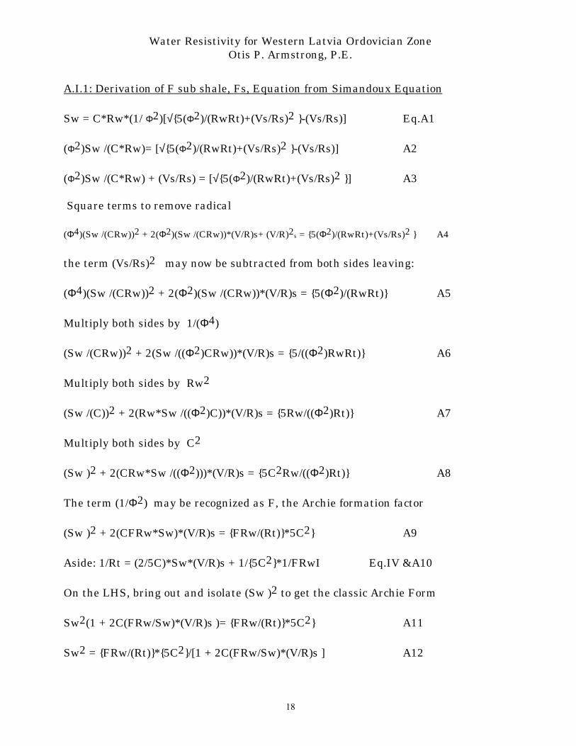
A.I.1: Derivation of F sub shale, Fs, Equation from Simandoux Equation Sw = C*Rw*(1/ Φ2)[√{5(Φ2)/(RwRt)+(Vs/Rs)2 }-(Vs/Rs)] Eq.A1 (Φ2)Sw /(C*Rw)= [√{5(Φ2)/(RwRt)+(Vs/Rs)2 }-(Vs/Rs)] A2 (Φ2)Sw /(C*Rw) + (Vs/Rs) = [√{5(Φ2)/(RwRt)+(Vs/Rs)2 }] A3 Square terms to remove radical (Φ4)(Sw /(CRw))2 + 2(Φ2)(Sw /(CRw))*(V/R)s+ (V/R)2s = {5(Φ2)/(RwRt)+(Vs/Rs)2 } A4 the term (Vs/Rs)2 may now be subtracted from both sides leaving: (Φ4)(Sw /(CRw))2 + 2(Φ2)(Sw /(CRw))*(V/R)s = {5(Φ2)/(RwRt)} A5 Multiply both sides by 1/(Φ4) (Sw /(CRw))2 + 2(Sw /((Φ2)CRw))*(V/R)s = {5/((Φ2)RwRt)} A6 Multiply both sides by Rw2 (Sw /(C))2 + 2(Rw*Sw /((Φ2)C))*(V/R)s = {5Rw/((Φ2)Rt)} A7 Multiply both sides by C2 (Sw )2 + 2(CRw*Sw /((Φ2)))*(V/R)s = {5C2Rw/((Φ2)Rt)} A8 The term (1/Φ2) may be recognized as F, the Archie formation factor (Sw )2 + 2(CFRw*Sw)*(V/R)s = {FRw/(Rt)}*5C2} A9 Aside: 1/Rt = (2/5C)*Sw*(V/R)s + 1/{5C2}*1/FRwI Eq.IV &A10 On the LHS, bring out and isolate (Sw )2 to get the classic Archie Form Sw2(1 + 2C(FRw/Sw)*(V/R)s )= {FRw/(Rt)}*5C2} A11 Sw2 = {FRw/(Rt)}*{5C2}/[1 + 2C(FRw/Sw)*(V/R)s ] A12


19

This is seen as the classic Sw Eqn with, Fs, called F sub shale.

Fs = {5C2}/[1 + 2C(FRw/Sw)*(V/R)s ] A13

Sw2 = Fs*F*Rw/(Rt) A14 An important secondary equation is the conductivity equation, arrived at from A9, starting with dividing both sides by (FRw )to get:

{5C2/(Rt) – (2CSw)(V/R)s} = (Sw )2/(FRw) A14b Equation 14b appears significant in two ways: First, the R.H.S. must always be positive, so the LHS must always be greater than or equal to zero. Thus evaluation of the LHS for sections where Sw=1, should give a check on validity of shale volumes and shale resistivity value. Second, when F becomes large and at low Sw levels, the RHS will approach zero. Which seems to form basis of so called “dual water, (1/Sw = 1/Sw-s+1/Sw-a)” models. For example calculation of Sw using the LHS leads to: Sw-s = 2.5C(R/V)s(1/Rt) A14d Compare A14d to the empirical Sw-s term of dual water Indonesian model:

Sw-s = {Vs(Vs/2-1)}*(Rs/Rt)½ & Vs =(Rs/Rt)α α=1 or 2-(2Rs/Rt)0.25 if Rs/Rt<0.5 The third conclusion from A14b, is that as Vs approaches 1, the RHS must approach zero for the open porosity goes to zero. In this case at Sw=1, then Rs = 0.4/C*(Rt)(Vs) Eqn A14C The results of A14C is that many instances, Rs, is taken simply as resistivity of an adjacent shale bed. This method is exceptionally simple, provided there are no geometrical effects such as washed out bore hole or thin beds, and sectional resistivity represents the type clay intermingled with the formation of interest. Asquith notes that montmorillonite and illite lower resistivity more than kalonite and chlorite shale. The key element of equation A13 and 14, is that permutations of Rt or Rxo may be rapidly calculated for Pickett plots. The method applied here is: given, ND; Neutron log Deflection, Vs, Rs, and Rw, then calculate Rt for Sw=1 and Sw= ½ these 2 points are then plotted at the total porosity, ND point, along with the deep resistivity value. A similar second plot of Rn using Rmf is produced to look for hydrocarbon mobility or for thin beds where the full value of deep resistivity would not develop. An example is given in Figures 9 and 10. The section from 905 to 980 m of Fig’s 9 and 10 bailed at approximately 1 ton oil per day and exhibits an oil static top pressure of about 40 psi above grade.


20

A.I.2: Determination of Rs & Rw When F is Known The conductivity equation for Laterolog may be reduced at Sw=1 to: Rw/Rt (5FC2) = 1 + 2CVs(FRw/Rs) or Eq.A15 F/Rt = FVs 2/(5CRs) + 1/(Rw5C2) Eq.A16 When data is plotted on these x, y coordinates as y=mx+b, then slope m and intercept b will calculate Rw and Rs. Rw = 1/(5bC2) and Rs = 2/(m5C) Eq.A17-a,b A.I.3. Determination of F from Shale Factors when Rw & Rs are known Consider the case of a porous solid mixed and consolidated with modest amounts of clay particles . If one measures the porosity of this solid by resistivity in a saline solution, the calculated porosity of the new solid would be increased, directly in proportion to the fraction of consolidated clay introduced. “In all cases… the effect (of clay or shale) is similar. The clay acts as a separate conductive path additional to that afforded by the saline solution in the rock pores” , Wylie pg.16. This effect was quantified by Wylie with the following conductivity equation: 1/Rt = A*Sw + 1/(F*Rw*I) + B Eq-1 Equating Wylie’s conductivity equation (for Laterolog) to Simandoux equation, Eqn.A10, one arrives at C=0.45 and the following conductivity equation, when Sw=1 : 1/Rt =~ 1/(FRw) + 0.9(V/R)s Eq.A18 F/Rt = 1/Rw + 0.9(F*Vs)/Rs & Rs=0.9/m Eq.A19a,b 1/F = Rw/Rt – 0.90*Rw*(V/R)s A20 or for Rn and Rmf 1/F = Rmf/Rn – 0.90Rmf*(V/R)s A21 A.I.4 Sectional Summary In summary, this appendix proposed an analysis of well log data by the Pickett Plot, (PP) while allowing for considerations about shale levels. The Picket Plot looks for anomalies in resistivity by plotting log of resistivity against Neutron tool deflections, ND. Once anomalies are noted on the PP, it is useful to have an estimate of the degree of water saturation. In most instances, the presence of shale reduces resistivity deflections. This in turn makes hydrocarbon detection more difficult on a PP. It was proposed to add 100% & 50% Sw points to the Picket plot using a re-arranged Simandoux equation.


21

APPENDIX II What follows are considerations on the parametric factors and paradigms related to shale section analysis. The result is to offer a more comprehensive parameter for application of shale analysis. Finally, it contrasts the overly cautious position taken by Asquith: “ if a geologist overestimates shale content, a water bearing zone may calculate like a hydrocarbon zone”. In contrast, if shale factors are ignored, potential hydrocarbon bearing sections may be overlooked. In zones of low shale factor the Simandoux equations calculate exactly like the classic water saturation equations and thus, there is no loss of functionality when applying the proposed method, as contrasted to an overly cautious approach. A.II.1 Conductivity Equation Review Wylie proposed the following conductivity model of porous media with shale acting as a parallel conductor to the water inside the pores. 1/Rt = A*Sw + 1/(F*Rw*I) + B Eq-I Wylie’s term B, represents conductivity thru paths involving clay only. Wylie states that “most often the clay is dispersed and B can be ignored, but that when there are thin or continuous clay streaks, B can be quite large”. The middle term is the standard conductivity term of porous media filled with conducting and non conducting phases. The first term is conductivity of brine filled pores and dispersed clay particles in series. Implicit in this equation is: “shale conductivity acts independent of the immersing water salinity”.. The middle term is the normal conductivity term when shale is ignored. Simandoux refined this concept into a widely accepted equation: Sw = C*Rw*(1/ Φ2)[√{5(Φ2)/(RwRt)+(Vs/Rs)2 }-(Vs/Rs)] Eq-II It was shown that Simandoux equation can be arranged as: 1/Rt = (2/5C)*Sw*(V/R)s + 1/{5C2}*1/{F*Rw*I} Eq-III In this form, it is clear Wylie’s B term was dropped. To the extent this equation is a close model of actual physical process for conductivity in porous media., it is possible to re-arrange the terms to analyze well log data, especially on the Picket plot as shown above. AII.2 Comparisons of Wylie Core Data to Simandoux Equations Wylie and the AAPG manual conclude that shale effects are marginal unless salinity levels exceed 0.3 o-m at 80F. For example, when plotting Wylie’s core analysis data for Burgan Sands, against Simandoux Equation with F~5 and between V/R=0.6 and


22

0.19 respectively, Figure 3, one could conclude that at low Rw values, shale has little effect on calculated Sw values. As is shown in Figure 3, for Rw less than 0.3, both Wylie’s data and Simandoux equation have a resistivity index close to 1. However, this is only true at small values of F. For low porosity formations this is not so. Possibly because the shale conductivity path is a greater % of the total conductive path. Notice when Sw=1 that F: observed, is Rt/Rw, then equation 1 is: Fa/Fo = 1 + 0.9(Fa)(Rw)(V/R)s Eq.IV When Fa/Fo vs F is plotted, Figure 4, it can be seen that at large Formation Factors (right hand side of Fig4), as with many carbonate systems, substantial errors can result, if shale corrections are ignored, even when water resistivity ranges 0.06 to 0,14, even with the modest shale values of Figure 4: Wylie presented some core analysis in the form of I vs Sw. This appendix shows that I can be calculated in terms of the shale factors, in which instance I is called Is, I sub shale. Is = {{1/(Sw2)}/[1 + 2C(FRw/Sw)*(V/R)s ]}*[1 + 2C(FRw)*(V/R)s ] A33 Some important parametric points come from the I sub shale equation: At Rw=0 or nearly 0.00, then Is = I = 1/(Sw2), for any F or (V/R)s At Sw =1 the Is = I = 1 for any F or (V/R)s or Rw As Sw approaches 0.00, I approaches 1/Sw for any F or (V/R)s or Rw As Sw decreases, the effective power of Sw will range between –2 & -1 Increases in either F or (V/R)s can offset any parametric rules for Rw This last point is illustrated by plotting Wylie core studies and a parametric change in F*(V/R)s, Figure 5. Again, to match Wylie’s core data, an F on the order of the Burgan Sands F, 5, is used. Figure 5 shows that with low F values studied by Wylie, there is not a need to correct for shale effects when water resistivity is less than 0.30. However, with modest F values, and (V/R)s, shale correction factors become more important. It is seen in Figure 5 at I = 3, an Sw of 60% is actually 50% and at I = 10, the un-corrected Sw is 32% vs the corrected value of 19%. Another paradigm proposed by Asquith, was “that for shale content to significantly affect log derived water saturations, shale content must be greater than 10 to 15%”. Figure 5 shows this statement to be inaccurate when open porosity falls below about 15%.For example, at 5% open porosity, ignoring shale effect, gives Sw =1, and at 10% open porosity, ignoring shale factors, one arrives at 30% Sw, based on a modest shale factor of between 9 and 13%. The correct parameter to define cut off points is Fs, not simply Vs.


23

A.II.3 Formation Resistance For Picket Plots Once formation water resistance, Rw , is known it is then possible to calculate the Formation Resistance, Rt based on the Simandoux variant of Wylie equation; given an assumption of formation lithology and porosity. (Sw)n = F*’Fs* (Rw/Rt) or Rt = F*’Fs’ (Rw/(Sw)n); Eqn V At Sw = 1.00, then (Sw)n = 1.00 = F’ (Rw/Rt) so Eqn VI Rt = F*’Fs*’ Rw /(Sw)2 F’s relates to porosity & lithology. Eqn VII For Pickett plots the Eqn is arranged to calculate Rt at Sw=1 and Sw = ½ so as to allow judgment of the degree of water saturation, while accounting for shale and open porosity effects. A.II.4 RESISTIVITY RATIO WITH SHALE CONSIDRATIONS One key consideration in log analysis is that formation factors cancel out when considering resistivity ratio’s in the same matrix, but with different fluids. However, when shale are present, Fs cannot cancel as does the standard F, unless Rmf = Rw. As a rule, only small sections of a well ever have zero SP. Typically mud is formulated more saline than formation waters to reduce clay swelling tendency and thereby maintain formation porosity. When Rmf does not equal Rw, or when Sw for the two sections are not equal, Fs does not cancel and consideration should be given to the ratio of Fs. For example, at Sw=1, Sw=1 = Fs*F*Rw/(Rt) = F’s*F*Rmf/Rxo giving: A22 a,b {5C2}/[1 + 2C(FRw/Sw)*(V/R)s ]*F*Rw/(Rt) = {5C2}/[1 + 2C(FRmf/Sw)*(V/R)s ]*F*Rmf/Rxo Since lithology and porosity are considered uniform, radial to the well bore, C and F cancel, leaving: {1}/[1 + 2C(FRw/Sw)*(V/R)s ]*Rw/(Rt) = {1}/[1 + 2C(FRmf/Sw)*(V/R)s ]*Rmf/Rxo Rw/Rmf = (Rt/Rxo) *[1 + 2C(FRw)*(V/R)s ]/[1 + 2C(FRmf)*(V/R)s ] A25 Considering a carbonate situation with F=100, Rw =0.12 Rmf = 0.1, C=0.45, and (V/R)s = 0.11, one arrives at Rw/Rmf = (Rt/Rxo) *[2.06 ]/[1.88] = 1.1 *(Rt/Rxo) Considering a sandstone situation with F=35, Rw =0.06 Rmf = 0.1, C=0.4, and (V/R)s = 0.05, one arrives at Rw/Rmf = (Rt/Rxo) *[1.084 ]/[1.14] = 0.95 *(Rt/Rxo)


24

The Table below uses data from Table 1 to estimate Ordovician water resistivity. These calculations arrive at Rw about 25% less than if shale factors are ignored. Ord Ord Ord Cmb Ord Ord RL Rn Rt/Rxo RL Rn Rt/Rxo avg 10.1 13.3 0.8 1.8 6.7 0.3F's 2.05 3.24 1.07 1.30 Rs 2.20 2.80Vs 0.21 0.12C 0.45 0.40F 90.00 30.00Rw 0.14 0.065Rmf 0.29 0.29V/Rs 0.10 0.04 Rmfc calc'd= 0.29Rwc calc'd= 0.14 A.II.5 RESISTIVITY INDEX WITH SHALE CONSIDRATIONS The resistivity index, I, is an important concept for log analysis. I = R”@”Sw/{R”@”Sw=1} = Rt/Ro = Rt/{FRw} = kSw^(-n) A27 Generally, k=1 and n = 2, although an analysis of Wylie’s’ core analysis for San Andres, Texas carbonate cores gave k=0.5 and n =2 where F =1.25/ϕ2.2 . A28 In the case where shale is involved, I can be defined as follows: Since the resistivity index, I, = {R”@”Sw}/(R”@”Sw=1) A29 Simandoux equation can be recast as: Rt = {5C2}{FRw/(Sw2)}/[1 + 2C(FRw/Sw)*(V/R)s ] A30 (R@Sw=1) = {5C2}{FRw/(1)}/[1 + 2C(FRw/1)*(V/R)s ] A31 {R@Sw} = {5C2}{FRw/(Sw2)}/[1 + 2C(FRw/Sw)*(V/R)s ] A32 Is = {{1/(Sw2)}/[1 + 2C(FRw/Sw)*(V/R)s ]}*[1 + 2C(FRw)*(V/R)s ] A33


25

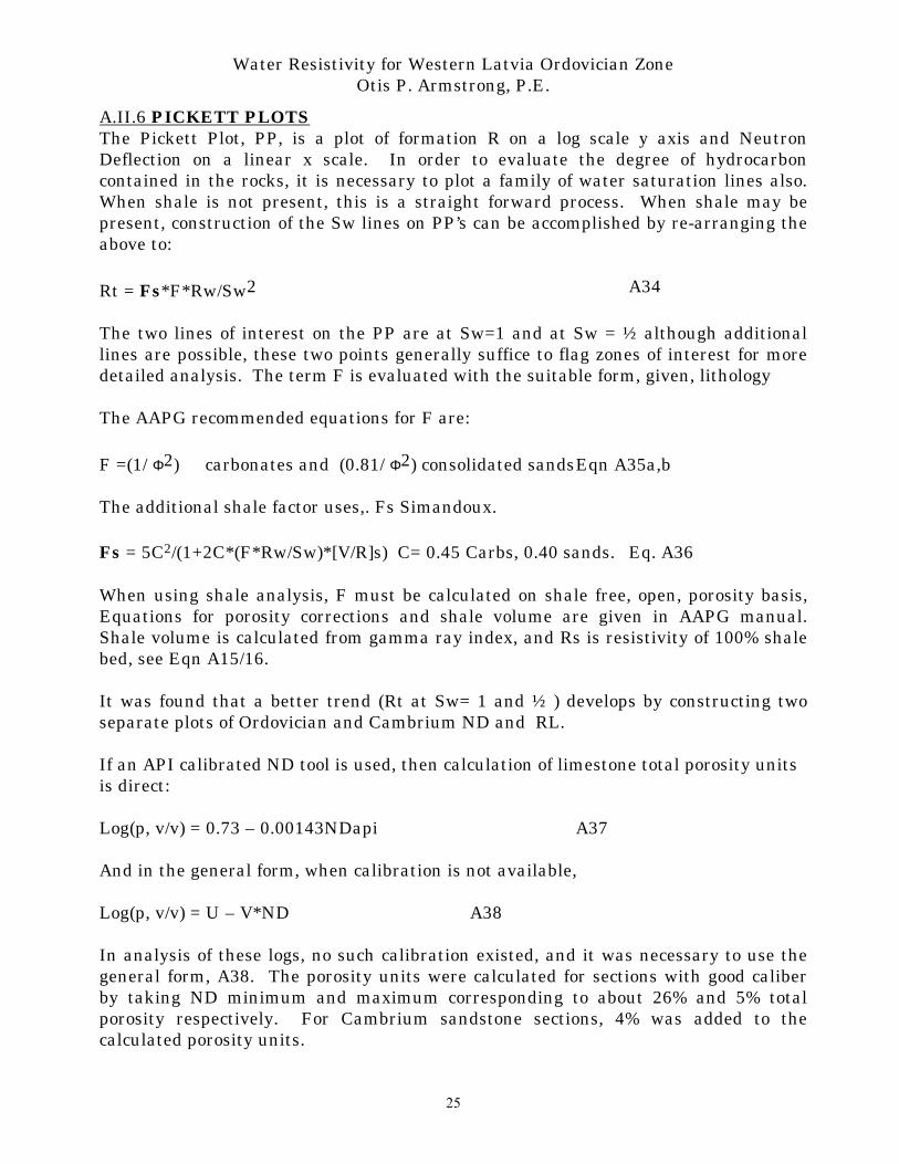
A.II.6 PICKETT PLOTS The Pickett Plot, PP, is a plot of formation R on a log scale y axis and Neutron Deflection on a linear x scale. In order to evaluate the degree of hydrocarbon contained in the rocks, it is necessary to plot a family of water saturation lines also. When shale is not present, this is a straight forward process. When shale may be present, construction of the Sw lines on PP’s can be accomplished by re-arranging the above to: Rt = Fs*F*Rw/Sw2 A34 The two lines of interest on the PP are at Sw=1 and at Sw = ½ although additional lines are possible, these two points generally suffice to flag zones of interest for more detailed analysis. The term F is evaluated with the suitable form, given, lithology The AAPG recommended equations for F are: F =(1/ Φ2) carbonates and (0.81/ Φ2) consolidated sands Eqn A35a,b The additional shale factor uses,. Fs Simandoux. Fs = 5C2/(1+2C*(F*Rw/Sw)*[V/R]s) C= 0.45 Carbs, 0.40 sands. Eq. A36 When using shale analysis, F must be calculated on shale free, open, porosity basis, Equations for porosity corrections and shale volume are given in AAPG manual. Shale volume is calculated from gamma ray index, and Rs is resistivity of 100% shale bed, see Eqn A15/16. It was found that a better trend (Rt at Sw= 1 and ½ ) develops by constructing two separate plots of Ordovician and Cambrium ND and RL. If an API calibrated ND tool is used, then calculation of limestone total porosity units is direct: Log(p, v/v) = 0.73 – 0.00143NDapi A37 And in the general form, when calibration is not available, Log(p, v/v) = U – V*ND A38 In analysis of these logs, no such calibration existed, and it was necessary to use the general form, A38. The porosity units were calculated for sections with good caliber by taking ND minimum and maximum corresponding to about 26% and 5% total porosity respectively. For Cambrium sandstone sections, 4% was added to the calculated porosity units.


26

The basic equations for PP analysis w/o shale factors are as follows: Given a regression line for SW =1 of the form: Log(Rt)= M*ND + B A39 At F =10, Rw = Rt/10, and Rmf = Rxo/10 A40a, b use Eq.A35a or b to calculate porosity for F=10, then apply A38 to get ND, and lastly, apply 40a,b to arrive at Rw or Rmf. When this method was applied to Ordovician section of 7 well logs, the average Rw was 0.13, with a range of 0.09 to 0.18 o-m. This method made an educated assumption about the porosity range. If Rw and Rs are known, as postulated by this paper, then either, the basic Archie or the Fs modification can be used to determine total porosity range and apply A38 to scale open porosity units. Once open porosity units are scaled to ND, then shale corrected R at Sw=1 and ½ points are plotted at each original ND along with log resistivity. For example see Figures 9 and 10. APPENDIX III Discussion of Porosity Factors Simply, there are two types of physical pores: 1) open pores which communicate flow (Vo) and 2) closed pores which do not communicate flow (Vc). Those which do not communicate flow can be by virtue of closure (poorly connected Vugs), by virtue of size (Micro Pores), and capillary action. Differentiation of these two pore types is loosely made by the terms “total porosity, φt” and “open porosity φo”. The total porosity being composed of the sum of the two terms Vo + Vc, which can be said to have a sum of 1, with a total matrix volume (Vt) being sum of solids, open holes and closed holes. Porosity is the fraction of pores to total volume: φt = (1)/Vt & φo = Vo/Vt , so φt/1 = φo/Vo =1/Vt & Vo=(1-Vc) so φo = φt*(1-Vc) In the case of a solid having a uniform pore fabric, with no vugs or micro pores, then open porosity is equal to total porosity. Sometimes, open porosity is taken as φo = φt*(1-Vc) or φo = φt*(1-Vsh). Where Vsh is volume of shale introduced, shale being a consolidated clay. This last equation is Asquith’s simple approach to correct φn-d for shale, pg 188, with results close to that obtained by more detailed methods.


27

Generally, porosity correction formula take the form: φo =φt - φtsVs. This forces the value of open porosity to zero at Vs =1, because tool response, φt , is φts at Vs=1. This correction is necessary because tool porosity response is calculated without regard to shale. Sometimes, shale density (2.4 to 2.8 g/cc) will be about equal to matrix density. In this case, no correction is required to the density porosity response. To a lesser extent, this may hold for sonic porosity, in the case of consolidated shale. Neutron tools respond to hydrogen content and the accepted calibration point for shale ranges between 30 (Schlumberger with 45% porosity adjacent clay, Asquith pg 103) and 33% (Wylie, pg 120). Wylie states that in sedimentary rocks there is virtually no non-effective porosity, i.e. all pores contain water directly interconnected with water in other pores.” However from a producing view point effective porosity is that quantity of pores which can contribute to fluid flow. Water contained by shale cannot contribute to flow due to the very low permeability factor. Likewise “connate water” cannot contribute to flow. Connate water in well log literature is often called Sw-irr. For flow calculations connate water is considered as rock, effective porosity would possibly be φe =(φt - φtsVs)*(1-Sw-irr). Hamada, Ref 15, considers there to be a lack of methodology in electrical logs to differentiate between shale waters and waters on pore walls held by static forces. Pirson17, presented a modified Wylie method (using electrical tools only) and calculates shale hydrated water as: Vws = (Rmf/Rw)Vsh – 1)/(Rmf/Rw-1) & calculate permeabilty by tortuosity method. For Pirsons’ example at Rmf=0.42, Rw=0.06 Vsh=0.71 and Sw=0.542, then Vws =0.497, the free water is 0.542-0.497 = 0.045 and the well completed with water free production. Summary: The proposed term, Fs; Eq. A36 is useful in defining the degree of impact shale factors can have on water saturation calculations. The apparent water (Rw*Fs)or apparent mud filtrate resistivity (Rmf*Fsxo) are useful diagnostic parameters when evaluating validity of ratio methods in shale sections.


28

Discussion of First Generation e-Log Tools Most Latvia e-log data are from a Normal (2 electrode) sonde N2M0.25A, plus a Lateral (3 electrode) sonde A2M0.25N. In some instances a 0.5m spacing was used for a Normal log. Characteristics of these first generation devices are seldom covered in modern geology. Modern logging tool has tools to read Rxo and Rt with a minimum of correction. There are 2 types of correction factors, environmental and geometric. Environmental factors are those factors relating to restivity of: mud Rm, formation Ri, invasion zone Ri, flushed zone Rxo, and shoulder Rs. Geometric factors are those related to hole diameter, sonde diameter, bed thickness, and invasion diameter. In both Normal and Lateral instruments, points A and B are current electrodes and M and N are voltage electrodes. For lateral Sonde AO=(AM+AN)/2 and investigation depth is about AO. Investigation depth is 2AM for the Normal sonde. Both sondes read V= (Ri/4*3.14)(1/AM-1/AN). In a USA Normal arrangement 1/AN is insignificant compared to 1/AM and V is taken as just (Ri/4*3.14)(1/AM). For LV normal sonde this is not the case. A feature of an unfocused sonde is current saturation. For lateral tool borehole correction is not significant for Ra/Rm<50, and Ra/Rm=Rt/Rm for all but extreem values of (s/dh) , sonde spacing/hole diameter. Likewise for the normal sonde borehole correction is not significant for Ra/Rm<10. But in front of a highly resistive beds or when the ratio of (s/dh) to is small, Rt/Rm will always be greater than Ra/Rm. Current saturation appears as the asymptotic value of Ra/Rm or Ra/Rs on departure charts, given a large value of ordinate value, Rt/Rm or Rt/Rs. Readings close to the asymptotic value should be considered unreliable.. For a 4 electrode lateral sonde, current is split: Rmax/Rmud= (8*(AO/dh)2)/(1-(ds/dh)2). For an 8.75” hole and a 75mm sonde of AO=32”, 126= Rmax/Rmud, Fig.9.3, Pirson. For a 3 electrode lateral sonde current is not split and Rmax/Rmud= (4*(AO/dh)2)/(1-(ds/dh)2). For an 8.0” hole and a 3.5” sonde of AO=18’8”, 825= Rmax/Rmud, Fig.2.15, p16, Hilchie. The formula for Normal sonde is Rmax/Rmud= (8*(AM/dh) (AN/dh))/(1-(ds/dh)2) and for Schlumberger sonde of AM=16”, AN=240” and a 3.5” sonde in a 16” hole Rmax/Rmud,=125, Fig 3.8, pg.24 Hilchie. This relationship shows why longer electrode spacing are less effected by hole diameter dh. These relationships allow determination of mud resistivity, given Rmax, dh, and ds or given Rmud, sonde spacing and diameter, determine hole diameter, below table. A short coming of the LV short normal arrangement is the relativly low saturation value, about 1/5 that of the US configuration. Corrections beyond 75% of the saturation value are too large to provide a reliable value. The below table list saturation values for the LV sondes in 8, 10, 16 inch holes.


29

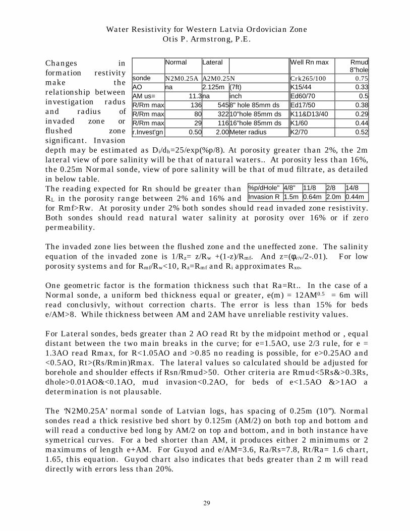
Changes in formation restivity make the relationship between investigation radus and radius of invaded zone or flushed zone significant. Invasion depth may be estimated as Di/dh=25/exp(%p/8). At porosity greater than 2%, the 2m lateral view of pore salinity will be that of natural waters.. At porosity less than 16%, the 0.25m Normal sonde, view of pore salinity will be that of mud filtrate, as detailed in below table. The reading expected for Rn should be greater than RL in the porosity range between 2% and 16% and for Rmf>Rw. At porosity under 2% both sondes should read invaded zone resistivity. Both sondes should read natural water salinity at porosity over 16% or if zero permeability. The invaded zone lies between the flushed zone and the uneffected zone. The salinity equation of the invaded zone is 1/Rz= z/Rw +(1-z)/Rmf. And z=(φv/v/2-.01). For low porosity systems and for Rmf/Rw<10, Rz=Rmf and Ri approximates Rxo. One geometric factor is the formation thickness such that Ra=Rt.. In the case of a Normal sonde, a uniform bed thickness equal or greater, e(m) = 12AM0.5 = 6m will read conclusivly, without correction charts. The error is less than 15% for beds e/AM>8. While thickness between AM and 2AM have unreliable restivity values. For Lateral sondes, beds greater than 2 AO read Rt by the midpoint method or , equal distant between the two main breaks in the curve; for e=1.5AO, use 2/3 rule, for e = 1.3AO read Rmax, for R<1.05AO and >0.85 no reading is possible, for e>0.25AO and <0.5AO, Rt>(Rs/Rmin)Rmax. The lateral values so calculated should be adjusted for borehole and shoulder effects if Rsn/Rmud>50. Other criteria are Rmud<5Rs&>0.3Rs, dhole>0.01AO&<0.1AO, mud invasion<0.2AO, for beds of e<1.5AO &>1AO a determination is not plausable. The ‘N2M0.25A’ normal sonde of Latvian logs, has spacing of 0.25m (10”). Normal sondes read a thick resistive bed short by 0.125m (AM/2) on both top and bottom and will read a conductive bed long by AM/2 on top and bottom, and in both instance have symetrical curves. For a bed shorter than AM, it produces either 2 minimums or 2 maximums of length e+AM. For Guyod and e/AM=3.6, Ra/Rs=7.8, Rt/Ra= 1.6 chart, 1.65, this equation. Guyod chart also indicates that beds greater than 2 m will read directly with errors less than 20%.

Normal Lateral Well Rn max Rmud 8”hole

sonde N2M0.25A A2M0.25N Crk265/100 0.75AO na 2.125m (7ft) K15/44 0.33AM us= 11.3na inch Ed60/70 0.5R/Rm max 136 5458" hole 85mm ds Ed17/50 0.38R/Rm max 80 32210"hole 85mm ds K11&D13/40 0.29R/Rm max 29 11616"hole 85mm ds K1/60 0.44r.Invest'gn 0.50 2.00Meter radius K2/70 0.52

%p/dHole" 4/8" 11/8 2/8 14/8 Invasion R 1.5m 0.64m 2.0m 0.44m


30

Sonde CF type Equation Nlong shoulder Rt/Ra=[(3.149/(e/AM)1.8)ln(Ra/Rs) + 1] e/AM>2 Guy. Fig3p139 N Ri/Rs=exp(3.28+.03Ra/Rs-.08e/AM) Pirson Nshort bore Ri/Rm=a(Ra/Rm)m m=1.28/(AM/dh)0.23

a=0.77+0.036(AM/dh) Sch 1-3AM/dh

Lat Rt/Ra=(a)e^(bRa/Rs) a=1.18-0.376e^(b), b=0.83(e/AO)0.56 . valid: 0.1>e/AO <1

Guy. Fig6p140

Lat shoulder S=3.45-1.53lnT; T=e/AO & A=[(Ra/Rs)/S-1]

Guy. Fig.6.19

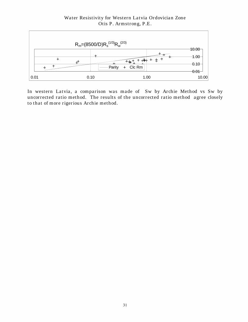
Rt/Rs=35exp(A(1.2T+4)) for e/AO<1 Guy. Fig.6.19 Pirson’s interpretation rules, for the normal sonde are as follows: Schlumberger give a chart for the short normal sonde regressed as follows: Fa=(Rn/Rm)1.22(AM/dh)-0.79(Rmf/Rw)0.33 or logFa=1.22log(Rn/Rm)-0.79log(AM/d)-.0042SP, where SP =-75log(Rmf/Rw)., for Rn/Rmud=7.9, AM/hole,d=2 and SP=-108mv, Fa=20.2, if zone is thought to be HC flushed use F=Fa/Si2, ie at 30% residual HC Si=0.7 & F=40.4.. For 30API oil ROS=%POR, double this for gas or low API and at 45API the values may be halved.. Interpertation of logs run with a short normal depends on the invaded zone, Si=√(FRz/Ri). In the instance only Rsn is reliable, Pirson proposed Sw=F/(aRi/Rmf). Where a =: z(Rmf/Rw-1)+1 and Ri is Rsn corrected for borehole and shoulder effects. It is based on Tixler Sxo eqn for Sw in the rocky mountian area, or Sxo equals root of Sw. The lateral sond will read a thick bed short by AO and also produce a shadow zone of AO length below bed top., and for e<AO will also produce a reflection peak below the bed at distance e+AO. A correction chart of Guyoid, Fig6.19 for Lateral sonde of e/AO <1 for resistive beds is as follows: T=e/AO, For Ra/Rs=2.9, T=0.75, Rt/Rs=10.1 vs 8.4 by chart. Reported valid for Rm>0.3Ra and <5Ra; dh>AO/100 and <AO/5; MN>AO/100 and <AO/5. Another Guyoid Lateral chart, Fig6p140, valid for e/AO<1 & >0.1. for e/AO=0.45, Ra/Rs= 4.14, Rt/Ra=4.2 chart, and 4.65 this equation. The chart below is an empirical fit, Rm=(8500/D)Rs

(1/3)Rw(2/3) of mud resistivity for a variety

of US wells, using predominately natural muds. It was inspired by Guyoids’ comment that Rs/Rm seldom exceeds 3. In this data set the median was 3, but ranged from 77 to 0.4, Depths 14400ft to 2500ft, Rw 0.3 to 0.01, Rs 7.0 to 0.40. In modern practice, the resistivity value of natural muds are modified to improve electric log accuracy. For Laterolog it is ideal for Rmf to equal Rw and for induction logging it is preferred that Rm exceed 3Rw.


31

Rm=(8500/D)Rs(1/3)Rw

(2/3)

0.01

0.10

1.00

10.00

0.01 0.10 1.00 10.00

Parity Clc Rm

In western Latvia, a comparison was made of Sw by Archie Method vs Sw by uncorrected ratio method. The results of the uncorrected ratio method agree closely to that of more rigerious Archie method.


32

References, Basic Materials 1. Special consideration is given to the Geological Specialists of Latvia for their

assistance in providing the basic details and digitized log, in hopes this report gives their work due consideration.

2. Asquith, G.B. Gibson, C.R. 1983, Basic Well Log Analysis, AAPG Tulsa 3. Craft & Hawkins 1957, Reservoir Engineering; Prentice Hall 4. Archie, Choquette, Robinson, et-al 1972, Carbonate Rocks II: Porosity and

Classification of Reservoir Rocks; AAPG Reprint series No.5; Tulsa Ok. 5. Heilander, P. 1982, Well Log Fundamentals, , Penwell Publications, Tulsa. 6. Wylie, M.R.J., 1963 The Fundamentals of Well Log Interpretation, 3rd Ed,

Academic Press, NYC 7. Patnode HW, Wylie, M.R.J, 1950, The Presence of Conductive Solids in Reservoir

Rock as a Factor in Electric Log Interpretation, Trans. AIME 189, 205, 47 8. Poupon A., Loy, ME, Tixier M.P.,1954 A Contribution to Electrical Log Interpretation in

Shaly Sands, Trans. AIME 201, 138, (“ A method for semi quantitative interpretation of E log in Shaly sand sections which are clean in themselves but contain stratified clay or shale)

9. de-Witte, AJ, (Mar4 & April 15, 1957), Saturation and Porosity from Electric Logs in Shaly Sands, O&GJ, 55 ( A method of computing oil saturation and porosity in formations which contain disseminated clay minerals, with simple Nomographs)

10. Simandoux, P, 1963, Mesures dielectriques en milieu poreux, application a mesure des saturations en eau: Eutde du Comportement des Massifs Argileux, "Dielectric Measurements on Porous Media, Application to the Measurement of water saturation, Study of the Behavior of Argillaceous formations,". in Revue de L’institut Francais du Petrole, Vol.18 Supplementary Issue, pp. 193-215 Translated in shaly-sand reprint volume, Part 4, SPWLA, Houston, pp. 97-124.

11. Asquith,G.B. Log Evaluations of Shaly Sandstones, A Practical Guide 1985 AAPG, Tulsa Ok.

12. El-M Shokir E.M,.April 23, 2001 Neural network determines shaly-sand hydrocarbon saturation, O&GJ, Oil&Gas Journal

13. Meehan, D.N. Vogel E.L., 1982, Reservoir Engineering Manual using HP41 pp 227-233, Penwell Publishing, Tulsa OK

14. Poupon A., Loy, Leveaux, J., May 1971, Evaluation of Water Saturation in Shaly Formations, SPWLA 12th Annual Logging Symposium (Presentation of the so called “Indonesia Dual water” model)

15. Hamada G.M. Et-al, Jan 1/01 Low Resistivity Beds May Produce Water Free, O&GJ Tulsa (a review of shale models plus example of E-log failure to detect producible zone, delineated by NMR log)

16. Connelly,W. Krug J. Nov 23/92: Russian Ventures, Western Siberia Opportunities – Evaluating Log and Core Data part 1/5: O&GJ, Tulsa (description of interpretation problems arising from differences between old Soviet era well log format & modern format)

17. Pirson, S.J., Formation Evaluation by Log Interpretation, World Oil GPC, Houston Tx April/May /June 1957, wide range of topics relative to older logs & oil/water mobility in various reservoir rock types, including shaly reserviors & non-wetting rocks

18. Guyod,H. Electrical Well Logging Fundamentals, Mostly reprints from World Oil & Oil Weekly 1944-1952 and one from O&GJ v.50No.31 Dec6/1952.


33

19. Guyod H. Electric Analogue of Resistivity Logging, Geophysics Vol.XXNo.3 July/1955 pp615-629

water resistivity for western latvia ordovician … resistivity for western latvia ordovician zone...

Documents