EUROPEAN COMMISSION

Sustainable Real Exchange Rates

in the New EU Member States:

Is FDI a Mixed Blessing?

Jan Babecký, Aleš Bulíř and Kateřina Šmídková

Economic Papers 368| March 2009

EUROPEAN ECONOMY

Economic Papers are written by the Staff of the Directorate-General for Economic and Financial Affairs, or by experts working in association with them. The Papers are intended to increase awareness of the technical work being done by staff and to seek comments and suggestions for further analysis. The views expressed are the author’s alone and do not necessarily correspond to those of the European Commission. Comments and enquiries should be addressed to: European Commission Directorate-General for Economic and Financial Affairs Publications B-1049 Brussels Belgium E-mail: Ecfin-Info@ec.europa.eu This paper exists in English only and can be downloaded from the website http://ec.europa.eu/economy_finance/publications A great deal of additional information is available on the Internet. It can be accessed through the Europa server (http://europa.eu ) KC-AI-09-368-EN-N ISBN 978-92-79-11179-2 ISSN 1725-3187 DOI 10.2765/25024 © European Communities, 2009

- 2 -

Sustainable Real Exchange Rates in the New EU Member States:

Is FDI a Mixed Blessing? Jan Babecký (Czech National Bank), Aleš Bulíř (International Monetary Fund) and Kateřina

Šmídková (Czech National Bank and Charles University)

Paper prepared for the Workshop: “Five years of an enlarged EU – a positive-sum game”

Brussels, 13-14 November 2008

Abstract This essay focuses on the various macroeconomic opportunities and challenges created by the foreign direct investment (FDI) inflows in the new member states (NMS). We question whether the macroeconomic performance of the NMS is furthered through the FDI’s overall positive impact on the trade balance or whether it can actually worsen the performance. Our findings suggest that in some NMS the integration gain, foreseen by the financial markets, may be reflected in a sustainable appreciation of the real exchange rate. Such real appreciation is in most cases moderate enough to allow for smooth nominal convergence required for to the euro adoption. In some cases, however, this appreciation is very fast, especially in the NMS with a low net external debt and massive FDI inflows, making it challenging to fulfill the Maastricht criteria. The Maastricht criteria may be difficult to meet also in those NMS where FDI has been channeled predominantly into services, housing construction, or nontradable sectors in general. In these countries we observe increasing net external debt without a corresponding improvement in the trade balance and these economies might be required to depreciate their currencies in real terms to sustain the external balance. JEL Classification Numbers: F31, F33, F36, F47 Key words: Foreign direct investment, new EU member states, euro adoption ____________________________

Acknowledgements: During our work we benefited from comments by Ignazio Angeloni, Martin Cincibuch, Zdeněk Čech, Carsten Detken, Balázs Égert, Vítor Gaspar, László Halpern, Katarina Juselius, Jan Kodera, Louis Kuijs, Kirsten Lommatzsch, Martin Mandel, Alessandro Rebucci, Istvan Szekely, Corina Weidinger Sosdean, and participants at seminars at the European Commission, European University Institute, International Monetary Fund, Prague University of Economics, Czech National Bank, and European Central Bank. Disclaimer: The views and opinions expressed here are the authors' only and should not be attributed to the European Commission. They do not necessarily correspond to those of the Czech National Bank or the International Monetary Fund

- 3 -

I. INTRODUCTION

Almost five years after the EU 2004 enlargement, the majority of the twelve new member states (NMS) that joined the EU in May 2004 (the Czech Republic, Cyprus, Estonia, Hungary, Latvia, Lithuania, Malta, Poland, Slovakia, and Slovenia) and in January 2007 (Bulgaria, Romania) are still in the process of catching-up to the EU level of development. Both processes, which are difficult to disentangle empirically, may have serious implications for macroeconomic policies of the NMS. Specifically, these processes may affect both the sustainable real exchange rates (SRER) and the observed ones (RER). Drawing a comprehensive overall picture requires taking into account various monetary frameworks (inflation targeting, hard pegs, currency board) employed by the NMS as well as their speed of the euro area accession (Slovenia, Cyprus, Malta, and Slovakia either have or will have adopted the euro, while the rest are still at least a few years away from that ultimate objective).

Our essay is motivated by a few selected stylized facts regarding the NMS and their real exchange rates. First, the currencies of the NMS currencies have appreciated substantially in real terms during the last decade. On average, the speed of real appreciation was very high at about 5 percent per year. Second, this appreciation either cannot be attributed to or it appears to contradict such frequently used justifications as excessive devaluation at the start of the transition process (Halpern and Wyplosz, 1997); significantly rising total factor productivity in the tradable-good sector due to the Balassa–Samuelson effect (Cincibuch, and Podpiera, 2004); or the external wealth accumulation hypothesis according to which the NMS’ sizable external liabilities require trade surpluses supported by a depreciated real exchange rate (Lane and Milesi-Ferretti, 2002). Third, NMS have received massive inflows of foreign direct investment (FDI) that may have affected investors’ perceptions about the countries’ long-term sustainable external balances.

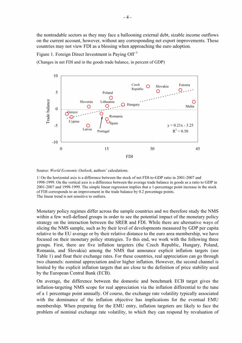
We suggest that FDI is the main culprit in explaining the real exchange rate appreciation, which is otherwise at odds with the above-mentioned traditional explanations for real appreciation (initial disequilibrium, the Balassa–Samuelson effect, and the external wealth accumulation hypothesis). Assuming that export growth and productivity improvements are driven by FDI—as compared to being a simple function of price competitiveness and external demand—contemporaneous capital inflows may signal expected future net export gains consistent with an appreciation in real exchange rates that will be long-lasting and that will sustain external balance. Clearly, the real appreciation is sustainable only if the net export gains are sufficient to prevent the increase of net external debt above some safe threshold. Of course, external debt may grow for a number of reasons, one of which is profit repatriation. The simple relationship between the increase in the stock of FDI and improvements in the trade balance in goods is suggestive—the NMS with the biggest FDI accumulation export more than those with small FDI accumulation (Figure 1).

On the one hand, the NMS that are successful in attracting FDI should be able to appreciate their currencies in real terms without jeopardizing the long-term sustainable development of their economies. On the other hand, fast and strong financial integration with the EU can be a mixed blessing for those NMS that aim at adopting euro soon. For them fast and sustainable medium-term real appreciation may complicate the EMU preparations since it conflicts with the nominal convergence requirements. In contrast, moderate sustainable appreciation may be compatible with the EMU entry preparations in which case financial integration, represented by FDI inflows, is a pure blessing for the recipient NMS. More difficult to appreciate is the impact on those countries that received FDI predominantly into

- 4 -

the nontradable sectors as they may face a ballooning external debt, sizable income outflows on the current account, however, without any corresponding net export improvements. These countries may not view FDI as a blessing when approaching the euro adoption.

Figure 1. Foreign Direct Investment is Paying Off 1/ (Changes in net FDI and in the goods trade balance, in percent of GDP)

y = 0.21x - 3.25R2 = 0.50

-10

-5

0

5

10

0 15 30 4

FDI

Trad

e ba

lanc

e sd

5

Portugal

Czech Republic

SloveniaHungary

Greece

Spain

Poland

Malta

Slovakia Estonia

Cyprus

Latvia

Romania

Lithuania

Source: World Economic Outlook, authors’ calculations.

1/ On the horizontal axis is a difference between the stock of net FDI-to-GDP ratio in 2001-2007 and 1998-1999. On the vertical axis is a difference between the average trade balance in goods as a ratio to GDP in 2001-2007 and 1998-1999. The simple linear regression implies that a 1-percentage point increase in the stock of FDI corresponds to an improvement in the trade balance by 0.2 percentage points. The linear trend is not sensitive to outliers.

Monetary policy regimes differ across the sample countries and we therefore study the NMS within a few well-defined groups in order to see the potential impact of the monetary policy strategy on the interaction between the SRER and FDI. While there are alternative ways of slicing the NMS sample, such as by their level of developments measured by GDP per capita relative to the EU average or by their relative distance to the euro area membership, we have focused on their monetary policy strategies. To this end, we work with the following three groups. First, there are five inflation targeters (the Czech Republic, Hungary, Poland, Romania, and Slovakia) among the NMS that announce explicit inflation targets (see Table 1) and float their exchange rates. For these countries, real appreciation can go through two channels: nominal appreciation and/or higher inflation. However, the second channel is limited by the explicit inflation targets that are close to the definition of price stability used by the European Central Bank (ECB).

On average, the difference between the domestic and benchmark ECB target gives the inflation-targeting NMS scope for real appreciation via the inflation differential to the tune of a 1 percentage point annually. Of course, the exchange rate volatility typically associated with the dominance of the inflation objective has implications for the eventual EMU membership. When preparing for the EMU entry, inflation targeters are likely to face the problem of nominal exchange rate volatility, to which they can respond by revaluation of

- 5 -

central parity of the ERM2 as was done in the past. However, not all countries that have declared inflation targeting as their monetary strategy are the full-fledged inflation targeters, some have employed what is called the inflation targeting “lite” strategy (Carare and Stone, 2003, and Stone, 2003). The lite targeters have a composite objective, typically an inflation target and an exchange rate stability objective and their inflation forecasts are not well anchored in a modeling framework. By intervening in the foreign exchange market they are likely to miss the inflation target more often, but their ERM2 chances could be enhanced by a more stable nominal exchange rate (the long-run real exchange rate dynamics is of course unaffected by the regime choice). Also, inflation targeters are not in the same stage of inflation targeting. For example, Slovakia will exit its inflation targeting strategy and adopt euro in 2009; Romania is an inflation targeting latecomer, having targeted inflation from 2005 and, hence, Romania’s stylized facts may not always correspond fully to the story of our IT group.

Table 1. Announced Inflation Targets

Country (Year of the IT introduction) 2008–09 2010 and beyond

Czech Republic (1998) 3.0 percent (±1 percent) 2.0 percent (±1 percent)

Hungary (2001) 3.0 percent (±1 percent) 3.0 percent (±1 percent)

Poland (1998) 2.5 percent (±1 percent) 2.5 percent (±1 percent)

Romania (2005) 3.8 percent in December 2008

3.5 percent in December 2009 (±1 percent)

Has not been announced

Slovakia (2001) Close, but less than 2 percent Close, but less than 2 percent

The euro area countries (1999)

Close, but less than 2 percent Close, but less than 2 percent

Source: The websites of the Czech National Bank, Magyar Nemzeti Bank, National Bank of Poland, National Bank of Romania, Slovak National Bank, and the European Central Bank. Stone (2003) classified Hungary, Poland, Romania, and Slovakia as lite targeters. The Czech Republic is a full-fledged targeter. The ECB is not formally an inflation targeting central bank, however, it is generally seen as a sophisticated price stability targeter.

Second, there are four NMS (Estonia, Lithuania, Bulgaria, and Latvia) that operate under either a currency board or a hard-peg regime that has not been readjusted for a considerable period of time. These countries have thus only one channel available to appreciate their currency in real terms vis-à-vis the euro, namely a higher inflation differential. As a result, they may have difficulties with the Maastricht criterion for inflation to which the policy response is a lot trickier than that to the volatile nominal exchange rates experienced by the inflation targeters. Note, however, that real appreciation is typically computed in effective terms and if the basket of trading partners is not completely dominated by the euro area countries, even hard-peggers can face some nominal effective exchange rate appreciation.

- 6 -

Third, there are three recent entrants into the euro area (Slovenia, Cyprus, and Malta) among the NMS. (Slovakia will have adopted the euro only on January 1, 2009 and is thus included in the inflation targeting groups instead.) We add also three forerunners (Greece, Spain, and Portugal) to this group in order to draw on their experience when discussing the interaction of FDI and the SRER in the NMS. We select Greece, Portugal and Spain since they are the closest in their GDP levels to the NMS. Other EU members that were significant receivers of FDI, such as Ireland, were already too developed in the time when our sample starts to form a comparable group (Barry, 2000). The size of our sample is thus 15 EU countries when we analyze stylized facts and 13 countries when we compute the SRER (the full data set is not available for Cyprus and Malta).

There are various approaches to assess the interaction of the FDI and SRER. Empirical papers, especially those based on the time-series, single-equation approach, have been inconclusive with respect to the direction of currency misalignment. While currencies were find overvalued using one set of variables, they were often found balanced or undervalued in another. The puzzling ambiguity was explained by Driver and Westaway (2005), who found that alternative methods of computing equilibrium real exchange rates work with different time horizons and hence most of the differences can be explained away by the horizons of the individual studies. Long-term studies have found transition country currencies typically undervalued, whereas medium-term studies have found them mostly overvalued. By choosing different measures of external equilibrium or different speeds of disequilibrium adjustment, the resulting estimates of real equilibrium rates can change easily. We therefore prefer to rely on structural medium-term model of sustainable real exchange rates.

The starting point for our methodology is a theoretical framework that links FDI and the SRER. In the next step, we proceed to a simplified empirical model. Subsequently, we update the overview of the FDI flows/stocks, trade balances, and real exchange rates for our 15 sample countries. We then estimate the SRER model for our restricted sample of 13 EU countries based on an updated set of economic fundamentals comparable to our previous research: net external debt, the stock of net FDI, terms of trade, international interest rates, and domestic and external demand variables. It is worth emphasizing that the set of economic fundamentals that determines SRER is broader than in the typical empirical studies of developed, fully-integrated EU economies, namely, the stock of FDI is added to capture the effects of integration and convergence. To obtain a wide range of plausible SRER estimates we produce them using both the previously estimated elasticities of export and import equations as well as newly produced estimates and calibrations.

We estimate both the current misalignment and future path for the SRER. First, we compute the indicator of misalignment that compares the SRER estimates with the observed values of the real effective exchange rates. This measure can be used to determine whether or not a certain group of the NMS is more prone to overvaluation or undervaluation of their domestic currencies.

Second, we project the SRER trajectory (conditional on the projection of the fundamental economic variables and on the assumption of the sustainable net external debt) five years ahead to pinpoint those countries that may have difficulties with stabilizing both inflation and the nominal exchange rate in the medium-term. Countries with such difficulties are easy to recognize in our framework. One group of affected countries has a sharply downward sloping SRER trajectory implying either fast nominal appreciation, high inflation, or both. The other group has an upward sloping SRER trajectory due to a negative integration gain that would imply a need to either depreciate the domestic currency or deflate the domestic economy by limiting absorption.

- 7 -

Third, we subject our results to robustness tests related to estimated/calibrated parameters as well as exogenous variables projections. This analysis results into interval estimates of both the misalignment indicators and SRER trajectories, allowing us to encompass the various issues relevant for the NMS. For example, it reflects the idea that once the NMS are approaching the EMU entry, their risk premium ought to be reduced by financial markets to reflect their new prominent status of the euro area members. It also tackles the problem of normative nature of the SRER, namely the need to define the sustainable level of net external debt. Given the uncertainty of this level, we prefer to work with alternative trajectories, as opposed to a single targeted debt value. The robustness analysis also illustrates that the NMS may face a less favorable international environment than in the last decade, and hence the real appreciation trends observed so far may not continue in the forthcoming years. Specifically, the analysis shows the potential impact of the current financial crises on the NMS by estimating the impact of falling foreign demand on the SRER.

Somewhat paradoxically, unfavorable external demand developments are likely to limit the tensions between the preparatory process for the euro adoption and the integration gain in the most successful FDI recipients. Should the external trade environment become less advantageous for the NMS, slowing demand for their exports, the scope for the sustainable real appreciation may be limited, offsetting the strong positive impact of FDI on trade balance.

We also suggest that positive FDI effects (the integration gain) are likely to be longer-lasting than the medium-term negative effects of misalignment and than the periods of sharp sustainable real appreciation. Our analysis focuses on the medium-term when the tradeoffs are likely to be the largest. If the impact of the initial, FDI-driven appreciation coincides with the preparatory process for the euro adoption, the integration-gain benefits may be limited in the medium term as the domestic currency may be pegged to the euro at an unfavorable rate or the costs of nominal convergence may be too high. After the period of medium-term adjustment, the integration gain may start playing a dominant role again. The first wave of the euro adopters and forerunners, such as Portugal or Greece, provide useful lessons for the NMS in this respect.

The paper is organized as follows. Section II presents stylized facts regarding the NMS and the control group of the forerunners, the area members that introduced euro prior to the EU 2004 enlargement. Section III discusses various approaches to analyzing the interaction of the FDI and real exchange rates, including the highly aggregated SRER methodology that is the focus of this paper. Section IV outlines a macroeconomic model of the real exchange rate and capital stock determination and its empirical counterpart. Section V describes the data set, the model calibrations and underlying estimates. Section VI shows our empirical results for the SRER model of the NMS and the control group. Section VII concludes by suggesting some policy implications of our findings.

- 8 -

II. STYLIZED FACTS

Looking at our three groups of new member countries—inflation targeters (IT), exchange rate peggers, and euro-area members—we see that the stylized facts do not tell the same story for all the NMS, even though certain trends appear to be common across the whole sample. Our data sample starts in 1995 and goes to 2007 and we use several data sources, all described in the Annex I.

The first common trend is the appreciation of the real effective exchange rate. We show two CPI-based real effective exchange rate calculations, one from the IMF and the other from NiGEM, both moving broadly in the same direction.1 While all sample countries show some real appreciation during 1995-2007, the speed differs a lot across the sample and it does not seem to be correlated with the choice of a particular monetary policy strategy. Overall, sample-period real appreciation ranged between 10 percent in the forerunner countries and the early entrants into the eurozone, and 40-80 percent in the hard-peg and IT countries. Only Slovenia’s estimates differ between the two data sources: while the NiGEM estimate shows a sizable gain in competitiveness (real depreciation) during 2003-07, the IMF estimate shows a marginal loss (real appreciation), the difference being most likely in the definition of the effective nominal exchange rate, each source presumably using a different trade matrix.

Without taking the concept of sustainable real appreciation into account, the differences in real appreciation could lead to a conclusion that the countries with massive real appreciation must have suffered from a loss in price competitiveness generating unsustainably large trade deficits and thus potentially endangering the macroeconomic stability2. However, the sample real GDP growth averaged 5 percent in 2001-07, with only Portugal and Malta lagging significantly. In contrast, the Baltic states, Bulgaria, Romania, and Slovakia grew significantly faster than the average. In constant US dollar per capita terms all countries showed fast growth, in particular during 2001-07. The fastest growth was in the Baltic states that quadrupled their GDP per capita between the early 1990s and 2007. Real appreciation in the NMS did not affect negatively real growth, in part owing to moderate unit labor cost (ULC) growth. The patter growth of unit labor cost (ULC) needs to be separated into the “volatile” 1990s and “stable” 2000s. During 2001-07 ULCs either remained stable or declined marginally in our sample countries, the only notable exception being Romania.

With respect to the trade balances, the modest real appreciation in the forerunner countries and the early entrants into the eurozone seems to worsen their trade balances only marginally. Whereas real appreciation in countries with hard pegs seemed to have worsened 1 NiGEM is the large-scale quarterly macroeconomic model of the world economy created and maintained by the London-based National Institute of Economic and Social Research (http://www.niesr.ac.uk). The model is essentially new-Keynesian in its approach, in that agents are presumed to be forward-looking in some markets, but nominal rigidities slow the process of adjustment to shocks. Linkages between countries take place through trade, financial market interactions, and movements in international stocks of assets.

2 As argued earlier, the Balassa-Samuelson effect and its resulting impact on the productivity growth are not enough to explain the appreciation phenomenon.

- 9 -

their trade balances significantly (most notably in Bulgaria from a small surplus in 1996-97 to staggering -25 percent of GDP in 2007), comparable real appreciation among inflation targeters had no visible negative impact on their trade balances and these actually improved in all of them but Romania, the late convert to inflation targeting.

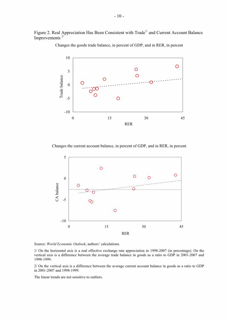
Current account balances deteriorated in most sample countries during 2001-07 and this deterioration was particularly pronounced in Spain and Greece and among hard peggers, the latter showing deficits to the tune of 15-25 percent of GDP. However, the IT group (with the exception of Romania) stabilized current account deficits at around 5 percent of GDP or less, with Romania’s deficit widening to almost 14 percent in 2007. To conclude, there is no clear bi-variate link between the speed of real appreciation and the size of trade and current account balances (Figure 2).

The previous results suggest that we should look at the factors behind the real appreciations more closely to see why in some countries fast real appreciation seems sustainable from the point of view of the external balance, while in others it leads to sizable external deficits. We will argue that FDI inflows may explain a substantial part of this puzzle.

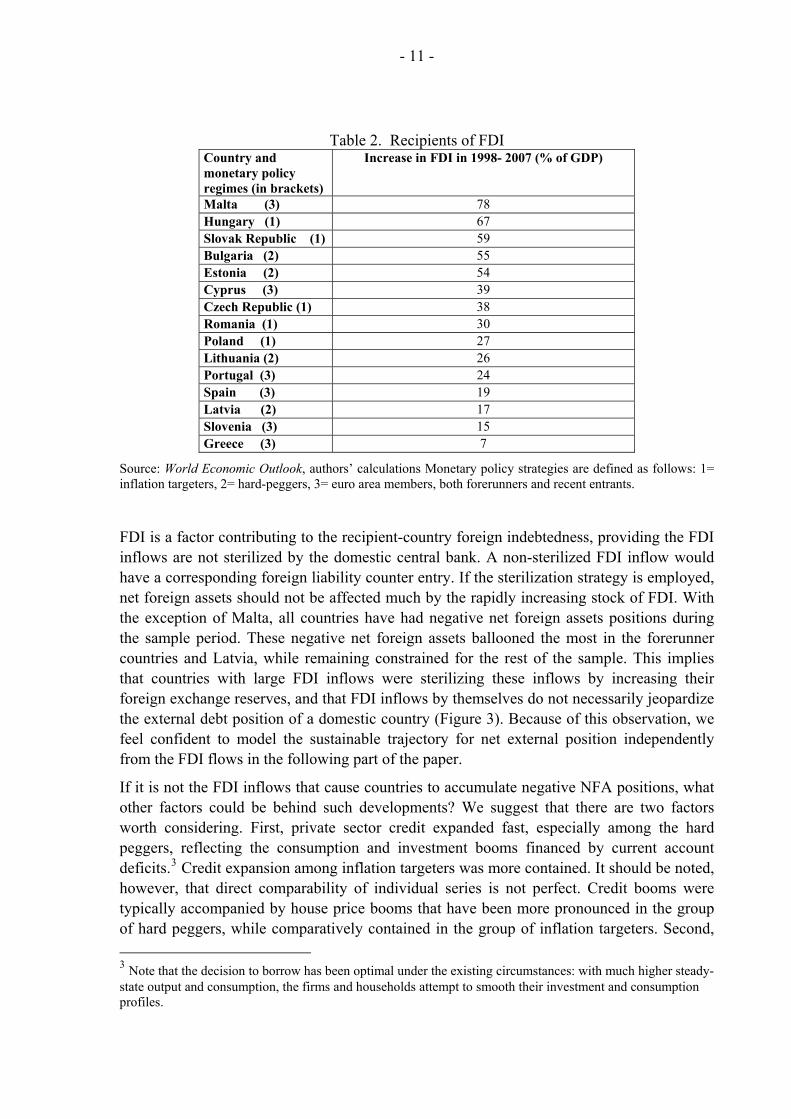
The stock of foreign direct investment grew fast in all countries, with the exception of Greece. However, only seven countries managed to accumulate a stock of FDI in excess of 50 percent of GDP. These countries belong to all three groups of countries—the eurozone, hard peg, and IT: Bulgaria, Cyprus, Czech Republic, Estonia, Hungary, Malta, and Slovakia. Six countries accumulated FDI equivalent to 25-50 percent of GDP, and two countries equivalent to 15-25 percent of GDP. A similar grouping arises when one looks at the increase in the FDI-to-GDP ratio. Seven countries (Bulgaria, Cyprus, Czech Republic, Estonia, Hungary, Malta, and Slovakia) attracted the new FDI of more than 30 percent of their GDP in the observed period (Table 2). From these data, it seems that the potential integration gain is related to neither a particular monetary policy strategy nor a particular exchange rate regime. If anything, there is some weak evidence that inflation targeters and countries outside the euro area were more successful in attracting the FDI. At the same time countries that attracted more FDI seem to exhibit faster real appreciation as well as smaller trade deficits as compared to the rest of the sample. This suggests that in their case, the faster real appreciation might have been sustainable.

- 10 -

Figure 2. Real Appreciation Has Been Consistent with Trade1/ and Current Account Balance Improvements 2/

Changes the goods trade balance, in percent of GDP, and in RER, in percent

-10

-5

0

5

10

0 15 30 4RER

Trad

e ba

lanc

e sd

5

Changes the current account balance, in percent of GDP, and in RER, in percent

-10

-5

0

5

0 15 30

RER

CA b

alan

ce sd

45

Source: World Economic Outlook, authors’ calculations.

1/ On the horizontal axis is a real effective exchange rate appreciation in 1998-2007 (in percentage). On the vertical axis is a difference between the average trade balance in goods as a ratio to GDP in 2001-2007 and 1998-1999.

2/ On the vertical axis is a difference between the average current account balance in goods as a ratio to GDP in 2001-2007 and 1998-1999.

The linear trends are not sensitive to outliers.

- 11 -

Table 2. Recipients of FDI Country and monetary policy regimes (in brackets)

Increase in FDI in 1998- 2007 (% of GDP)

Malta (3) 78 Hungary (1) 67 Slovak Republic (1) 59 Bulgaria (2) 55 Estonia (2) 54 Cyprus (3) 39 Czech Republic (1) 38 Romania (1) 30 Poland (1) 27 Lithuania (2) 26 Portugal (3) 24 Spain (3) 19 Latvia (2) 17 Slovenia (3) 15 Greece (3) 7

Source: World Economic Outlook, authors’ calculations Monetary policy strategies are defined as follows: 1= inflation targeters, 2= hard-peggers, 3= euro area members, both forerunners and recent entrants.

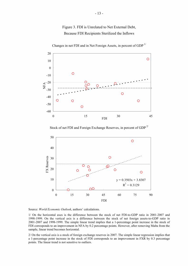
FDI is a factor contributing to the recipient-country foreign indebtedness, providing the FDI inflows are not sterilized by the domestic central bank. A non-sterilized FDI inflow would have a corresponding foreign liability counter entry. If the sterilization strategy is employed, net foreign assets should not be affected much by the rapidly increasing stock of FDI. With the exception of Malta, all countries have had negative net foreign assets positions during the sample period. These negative net foreign assets ballooned the most in the forerunner countries and Latvia, while remaining constrained for the rest of the sample. This implies that countries with large FDI inflows were sterilizing these inflows by increasing their foreign exchange reserves, and that FDI inflows by themselves do not necessarily jeopardize the external debt position of a domestic country (Figure 3). Because of this observation, we feel confident to model the sustainable trajectory for net external position independently from the FDI flows in the following part of the paper.

If it is not the FDI inflows that cause countries to accumulate negative NFA positions, what other factors could be behind such developments? We suggest that there are two factors worth considering. First, private sector credit expanded fast, especially among the hard peggers, reflecting the consumption and investment booms financed by current account deficits.3 Credit expansion among inflation targeters was more contained. It should be noted, however, that direct comparability of individual series is not perfect. Credit booms were typically accompanied by house price booms that have been more pronounced in the group of hard peggers, while comparatively contained in the group of inflation targeters. Second, 3 Note that the decision to borrow has been optimal under the existing circumstances: with much higher steady-state output and consumption, the firms and households attempt to smooth their investment and consumption profiles.

- 12 -

government balances also contributed mildly to the external debt in some cases. On average, central government balances—with the exception of Hungary—showed gradual consolidation, mostly related to the cyclical position of economies in question. Some of the hard peggers ran sizable surpluses, while all inflation targeters ran gradually narrowing deficits.

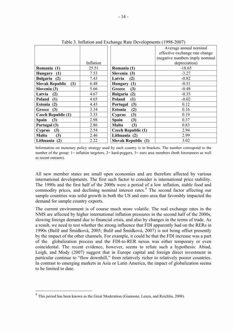
As we noted earlier, the monetary policy strategy may limit the scope for alternative channels to effect the real exchange rate appreciation. Inflation performance in our sample countries, when compared to their nominal effective appreciation rates, may suggests which channels were more important for respective groups (Table 3). While it is clear that there is a tradeoff between the two channels, and that countries with low inflation record exhibit stronger nominal effective appreciation, the link to the selected monetary strategy seems far from straightforward. In addition to reasons mentioned in the introduction (pure versus lite IT and euro versus effective exchange rate), the explanation can be found in the adoption dates of the strategy. For example, the Czech Republic introduced inflation targeting in 1998, while Romania only in 2005 and the inflation record has differed across the sample countries. Two forerunners (Portugal, and Spain), two euro area countries (Cyprus, and Malta) and Lithuania managed to keep their year-on-year inflation under 3 percent on average during 1998-2007. Five countries (Latvia, Poland, Estonia, Greece, and Czech Republic) kept inflation on average between 3 and 5 percent in 1998-2007. The remaining five countries did not keep inflation under the 5 percent level. Peggers brought inflation down quickly in the late 1990s, however, it accelerated above 5 percent in all of them in 2004 or shortly thereafter. Disinflation among inflation targeters was both more gradual and longer lasting—the only substantial acceleration in inflation in this group was recorder by Hungary.

- 13 -

Figure 3. FDI is Unrelated to Net External Debt,

Because FDI Recipients Sterilized the Inflows

Changes in net FDI and in Net Foreign Assets, in percent of GDP 1/

-60

-50

-40

-30

-20

-10

0

10

20

0 15 30FDI

NFA

sd

45

Stock of net FDI and Foreign Exchange Reserves, in percent of GDP 2/

y = 0.3503x + 3.8307R2 = 0.3129

0

10

20

30

40

50

0 15 30 45 60 75 9

FDI

FX R

eser

ves

0

Source: World Economic Outlook, authors’ calculations.

1/ On the horizontal axes is the difference between the stock of net FDI-to-GDP ratio in 2001-2007 and 1998-1999. On the vertical axis is a difference between the stock of net foreign assets-to-GDP ratio in 2001-2007 and 1998-1999. The simple linear trend implies that a 1-percentage point increase in the stock of FDI corresponds to an improvement in NFA by 0.2 percentage points. However, after removing Malta from the sample, linear trend becomes horizontal.

2/ On the vertical axis is a stock of foreign exchange reserves in 2007. The simple linear regression implies that a 1-percentage point increase in the stock of FDI corresponds to an improvement in FXR by 0.3 percentage points. The linear trend is not sensitive to outliers.

- 14 -

Table 3. Inflation and Exchange Rate Developments (1998-2007)

Inflation

Average annual nominal effective exchange rate change

(negative numbers imply nominal depreciation)

Romania (1) 25.51 Romania (1) -18.65 Hungary (1) 7.53 Slovenia (3) -3.27 Bulgaria (2) 7.43 Latvia (2) -0.82 Slovak Republic (1) 6.48 Hungary (1) -0.51 Slovenia (3) 5.66 Greece (3) -0.48 Latvia (2) 4.67 Bulgaria (2) -0.35 Poland (1) 4.65 Poland (1) -0.02 Estonia (2) 4.43 Portugal (3) 0.12 Greece (3) 3.34 Estonia (2) 0.16 Czech Republic (1) 3.33 Cyprus (3) 0.19 Spain (3) 2.98 Spain (3) 0.37 Portugal (3) 2.86 Malta (3) 0.83 Cyprus (3) 2.54 Czech Republic (1) 2.94 Malta (3) 2.46 Lithuania (2) 2.99 Lithuania (2) 2.22 Slovak Republic (1) 3.02

Information on monetary policy strategy used by each country is in brackets. The number correspond to the number of the group: 1= inflation targeters, 2= hard-peggers, 3= euro area members (both forerunners as well as recent entrants).

All new member states are small open economies and are therefore affected by various international developments. The first such factor to consider is international price stability. The 1990s and the first half of the 2000s were a period of a low inflation, stable food and commodity prices, and declining nominal interest rates.4 The second factor affecting our sample countries was solid growth in both the US and euro area that favorably impacted the demand for sample country exports.

The current environment is of course much more volatile. The real exchange rates in the NMS are affected by higher international inflation pressures in the second half of the 2000s, slowing foreign demand due to financial crisis, and also by changes in the terms of trade. As a result, we need to test whether the strong influence that FDI apparently had on the RERs in 1990s (Bulíř and Šmídková, 2005; Bulíř and Šmídková, 2007) is not being offset presently by the impact of the other channels. For example, it could be that the FDI increase was a part of the globalization process and the FDI-to-RER nexus was either temporary or even coincidental. The recent evidence, however, seems to refute such a hypothesis: Abiad, Leigh, and Mody (2007) suggest that in Europe capital and foreign direct investment in particular continue to “flow downhill,” from relatively richer to relatively poorer countries. In contrast to emerging markets in Asia or Latin America, the impact of globalization seems to be limited to date.

4 This period has been known as the Great Moderation (Giannone, Lenza, and Reichlin, 2008).

- 15 -

III. ANALYZING REAL EXCHANGE RATES AND FDI IN NMS

Stylized facts show clearly that NMS must take the interactions between real exchange rates and FDI inflows into account. They cannot assume that real exchange rates will be stable in the process of financial integration with the EU that brings massive FDI inflows to most of the NMS. Neither can they automatically assume that real exchange rate appreciation is sustainable in the medium-term no matter what the net external debt or international environment is. It is therefore important to analyze these interactions and decipher which real exchange rate changes are sustainable and which changes have policy implications for the NMS preparing for the euro adoption.

Our approach, explained in more detail in next part of the paper, defines the SRER as a real exchange rate that ensures a net external debt is sustainable in medium-term. This concept distinguish real exchange rate changes that are due to fundamental factors such as foreign demand for exports, initial external debt and FDI inflows from changes that are due to various short-term factors. The sustainability is a normative concept that depends on our definition of the steady-state level of net external debt. This steady-state level is taken from the empirical study that produced benchmarks for various types of economies. The more the current level of net external debt departs from its steady-state level, the more can real exchange rate deviate from the SRER.

The SRER concept is rooted in the pioneering studies that developed the empirical concept equilibrium (fundamental) real exchange rates (Williamson, 1994). There are various approaches to estimating equilibrium real exchange rates that work with different sets of fundamental variables and different time horizons (Driver and Westaway, 2005). Our approach belongs to the medium-term methodologies that work with both stock as well as flow variables. In comparison to previously applied methodologies, we put more emphasis on the role of FDI. Also, we implement the country-specific definition of sustainable external balance that reflects the fact that countries with favorable initial net external debts and recipients of massive FDI inflows can afford faster real appreciation in the medium-term while countries les lucky (with high initial debt levels or less FDI) face higher risks of overvaluation.

The advantage of the SRER approach is that is provides an aggregated framework for discussion about interaction of the real exchange rates and FDI. Alternative approaches provide an insight into several important issues that go beyond the scope of the SRER concept. First of all, there are alternative hypothesis explaining why the NMS experienced sharp real appreciation of their exchange rates. We have already mentioned the excessive devaluation at the start of the transition process and the Balassa–Samuelson effect that is based on interaction between the tradable and non-tradable sectors. According to various empirical studies, the Balassa-Samuelson effect plays a very limited role in driving real exchange rate appretiation in NMS (Cincibuch and Podpiera, 2004 and Égert, 2002). In addition, recent studies on globalization also claim that global prices are increasingly more important determinants of domestic price-setting behaviour for non-tradable goods (Borio andFilardo, 2006).

Additional complication when the Balassa-Samuelson effect is employed to explain the shar real appreciation in the NMS is the problematic empirical distinction between tradable and nontradable sectors. A firm may produce both types of products, or some notionally tradable goods are not really traded as they are directed primarily at the domestic market. Empirical studies available for the NMS suggest that no clear distinction can be made between tradable

- 16 -

and non-tradable goods, the 'degree of non-tradability' varying between 10 and 85 percent (Čihák and Holub, 2005). Also, Goldstein and Lardy (2005) use the example of car manufacturing in China that is predominantly serving the domestic market. Indeed, sectors producing tradable goods for the domestic market and for export tend to be fairly distinct in most newly industrialized and emerging or development countries.

The second important issue that goes beyond the scope of the SRER model is the non-homogeneity of the FDI. The impact of the FDI on the economy, trade balance and the real exchange rates depends on the capacity of domestic economy to absorb potential benefits and on recipient sectors. Hence, the impact is both country- as well as time-specific.

FDI has grown rapidly throughout the world in the last two decades, especially in developing countries, where it now accounts for almost half of total inflows (Kose et al., 2006). There is a strong presumption that FDI has a positive effect on economic growth and productivity through the transfer of technology and skills and by augmenting the recipient’s domestic capital stock. The aggregate-data support the evidence regarding the positive growth effect of FDI. However, FDI inflows seem to contribute to growth only in countries with a high level of human capital beyond a certain threshold (Borensztein, Degregorio, and Lee, 1998), when countries have well-developed financial markets (Alfaro et al., 2004), or in those with sufficient provision of infrastructure (Kinoshita and Liu, 2007). FDI contributes to economic growth by augmenting capital accumulation (Mody and Murshid, 2005) as evidenced by a strong “crowding-in” effect of FDI on domestic investment in developing countries between 1979 and 1999. Finally, the sectoral composition of FDI matters as positive externalities are realized through interactions between the sector receiving FDI and the rest of the economy. However, the evidence seems to suggest that if FDI is limited to the primary sector, the economy-wide externalities are smaller than if FDI concentrates in the manufacturing sector (Aykut and Sayek, 2007).

Differential effects have been observed for the earlier FDI waves (see, for example, the historic overview in Baldwin and Martin (1999). Specifically, the first wave of FDI in the early 1990s—an example of which is the Volkswagen’s bold purchase of the Czech carmaker Škoda—capitalized on the low wage level and a potential for productivity gains in the NMS (Lansbury, Pain and Šmídková, 1996) and was directed primarily into sectors producing tradable goods and services. In the early 1990s, in part owing to sharply devalued exchange rates in the transition countries, it would not make much sense to invest into nontradable sectors: the purchasing power of domestic population was low and they distrusted domestically produced goods. In a sense, this FDI wave was a repetition of the much earlier wave observed during the pre-WW I period (Baldwin and Martin, 1999). The second wave occurred in the late 1990s and early 2000s, with the process of real convergence well underway. With per capita incomes rising fast and the prospect of the EU accession looming, the flow of FDI was at least partly re-directed into the sectors producing nontradable goods and services. Especially financial services were a big recipient of these inflows, fueling the credit boom (International Monetary Fund, 2008).

Although it could be useful for the reasons mentioned above to distinguish the tradable and non-tradable FDI projects in the SRER model, it is extremely difficult to create a corresponding database. The data and measurement issues seem insurmountable. First, no such aggregate database exists, necessitating using primary sources, classification standards of which differ substantially across countries. Second, all difficulties with defining tradables and non-tradables mentioned in the context of Balassa-Samuelson effect apply here as well. The third issue related to the interaction of the real exchange rates and FDI is the measure of financial integration itself. The degree of financial integration can be measured either by

- 17 -

quantitative indicators that compare volumes of capital inflows to the level of domestic product or by qualitative indicators that estimate price convergence or by (Baltzer, Cappiello, De Santis, and Manganelli 2008). Our choice of the approximation of the integration process is given by the fact that the FDI brings capital, new technologies and management skills in the recipient economies (Sylwester, 2005, and Hunya, Holzner, and Wörz, 2007). The empirical effects of price convergence on exports and imports are not so well established. Similarly, the link between the total capital inflows and productivity of the real economy in the recipient country is supported by empirical studies less than the link between FDI and real economy. Moreover, the FDI stock is more homogenous variable than the total capital inflows.

IV. DERIVING THE EMPIRICAL MODEL OF FDI-DRIVEN REAL EXCHANGE RATES

We motivate the empirical estimates with a simple dynamic model of a small, open economy, the real exchange rate developments of which are affected by foreign direct investment.5 FDI has exercised a powerful effect on transition economies, both by stimulating aggregate supply and by raising permanent income. The two main channels of the impact of FDI on growth are well researched: first, through an increase in total investment and, second, through interaction of the FDI’s more advanced technology with the host’s human capital (Borensztein et al., 1998, and Lim, 2001).6 The literature has offered, however, limited agreement on the quantitative importance of those effects, especially in light of measurement issues and various counteracting processes discussed earlier. In the model below we focus on the former effect of capital accumulation, modeling an overall positive effect of FDI inflows on net exports (Holland and Pain, 1998; for the original presentation of the theoretical model see Bulíř and Šmídková, 2005). Theoretical model In the model—which resembles that of Blanchard (1981)—FDI is equally productive as domestic capital, contributing to capital accumulation. The impact of FDI can be modeled through standard money- and goods-equilibrium schedules, a classical production function, and uncovered interest parity (see also Annex II). Let us denote them as follows, with lower-case variables representing logarithms: (1) Rypm βα −=− , (LM) (2) , (IS) fygcky ρλψδγ ++++= *&

where m is the money supply; p is the price level; y and y* are domestic and world output, respectively (y* is external demand unrelated to the real exchange rate); R and R* are the domestic and world nominal interest rate, respectively; k is the stock of capital, with

5 The model does not incorporate any common-currency effect on trade and income (Frankel and Rose, 2002, or Bun and Klaasen, 2002) as the integration of the accession countries with their EU trading partners is assumed to have progressed towards the EU levels. Therefore, a common currency itself is not expected to bring about a significant integration gain.

6 To the extent the latter channel affects sectoral productivity, it is akin to the Balassa-Samuelson effect.

- 18 -

dtdk

kk 1≡& and t denoting time; c is the real exchange rate; g is the fiscal impulse; and f is

foreign direct investment. Greek characters stand for nonnegative and fixed parameters (all smaller than one). Output is increasing in the stock of foreign direct investment, f, above and beyond the increase in the capital stock, primarily because FDI generates substantial spillovers outside of its sectoral allocation. The IS curve can be thought of as a demand schedule of the usual type (income = consumption + investment + net exports), with g capturing the impact of public consumption and investment on demand and c and y* capturing the impact of external price and demand developments, respectively. (For simplicity, we assume that the impact of private consumption on demand is zero.) The coefficients δ, λ, and ρ can be thought of as the price, income, and FDI elasticities in a reduced-form, net export equation. As such, equation (2) corresponds to the empirical equations estimated below. On the supply side physical output is governed by a classical production function: (3) ky ε= , where , that is, the capital stock, k, is composed of “domestic” capital, i, and “foreign” capital, f, both of which have identical productivity at the margin.

fik +≡

Latecomer countries that have suboptimal capital stock accumulate capital faster than advanced countries with an optimal capital stock. Once the capital stock approaches its optimal level, the accumulation process slows down. Total debt is constrained in a debt accumulation schedule, where total debt is accumulated by FDI inflows and fiscal deficits, decrease with domestic growth, and is predetermined by its initial level. Capital accumulation is thus assumed to be decreasing in the existing stock of capital, the real interest rate, and, owing to crowding out, in total debt, d:

(4) ⎩⎨⎧

−−−=⇒≥−−−=⇒<

dkrtkkkdkrtkkk

ηφθϖηφθο

&

&

**

We have observed that countries with a suboptimal capital stock ( ), that is, latecomers, accumulate capital faster than advanced countries with an optimal capital stock ( , where

*kk <

*kk ≥ ** yk is constant) and, hence, ϖο > . Once the capital stock approaches its optimal level, the accumulation process slows down. Total debt is constrained in a debt accumulation schedule, where total debt is accumulated by FDI inflows and fiscal deficits, g, decrease with domestic growth, and, moreover, each country’s debt is predetermined by its initial level, d : (5) gfydd ικμ ++−= In other words, we assume that foreign investors care about the transition country’s growth prospects, return on FDI, and overall prospects of servicing its obligations (Campos and Kinoshita, 2003 or Bevan and Estrin, 2004). It is reasonable to assume that the other commonly used determinants of FDI inflows (lower wages, market attractiveness, “cultural distance,” and so on) are met in the countries in question.

- 19 -

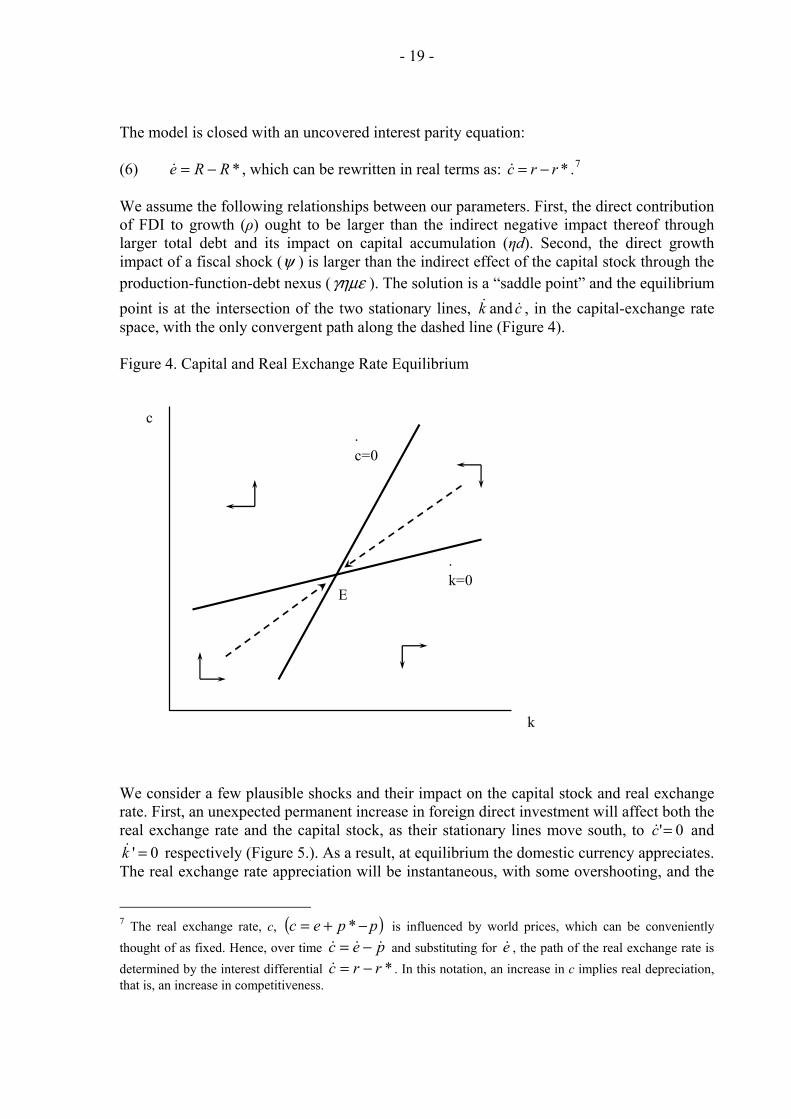
The model is closed with an uncovered interest parity equation: (6) , which can be rewritten in real terms as: .*RRe −=& *rrc −=& 7 We assume the following relationships between our parameters. First, the direct contribution of FDI to growth (ρ) ought to be larger than the indirect negative impact thereof through larger total debt and its impact on capital accumulation (ηd). Second, the direct growth impact of a fiscal shock (ψ ) is larger than the indirect effect of the capital stock through the production-function-debt nexus (γημε ). The solution is a “saddle point” and the equilibrium point is at the intersection of the two stationary lines, k and , in the capital-exchange rate space, with the only convergent path along the dashed line (Figure 4).

& c&

Figure 4. Capital and Real Exchange Rate Equilibrium

E

k

c

.k=0

.c=0

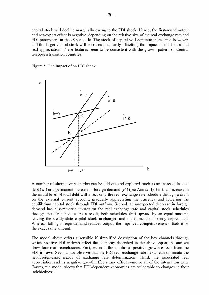
We consider a few plausible shocks and their impact on the capital stock and real exchange rate. First, an unexpected permanent increase in foreign direct investment will affect both the real exchange rate and the capital stock, as their stationary lines move south, to and

respectively (Figure 5.). As a result, at equilibrium the domestic currency appreciates. The real exchange rate appreciation will be instantaneous, with some overshooting, and the

0'=c&' 0k =&

)7 The real exchange rate, c, is influenced by world prices, which can be conveniently

thought of as fixed. Hence, over time and substituting for , the path of the real exchange rate is determined by the interest differential . In this notation, an increase in c implies real depreciation, that is, an increase in competitiveness.

( ppec −+= *pec &&& −=*rrc −=&

e&

- 20 -

capital stock will decline marginally owing to the FDI shock. Hence, the first-round output and net-export effect is negative, depending on the relative size of the real exchange rate and FDI parameters in the IS schedule. The stock of capital will continue increasing, however, and the larger capital stock will boost output, partly offsetting the impact of the first-round real appreciation. These features seem to be consistent with the growth pattern of Central European transition countries.

Figure 5. The Impact of an FDI shock

E'

k

c

.k'=0

.c'=0

.c=0

.k=0

k*k*'

E

A number of alternative scenarios can be laid out and explored, such as an increase in total debt ( d ) or a permanent increase in foreign demand (y*) (see Annex II). First, an increase in the initial level of total debt will affect only the real exchange rate schedule through a drain on the external current account, gradually appreciating the currency and lowering the equilibrium capital stock through FDI outflow. Second, an unexpected decrease in foreign demand has a symmetric impact on the real exchange rate and capital stock schedules through the LM schedule. As a result, both schedules shift upward by an equal amount, leaving the steady-state capital stock unchanged and the domestic currency depreciated. Whereas falling foreign demand reduced output, the improved competitiveness offsets it by the exact same amount. The model above offers a sensible if simplified description of the key channels through which positive FDI inflows affect the economy described in the above equations and we draw four main conclusions. First, we note the additional positive growth effects from the FDI inflows. Second, we observe that the FDI-real exchange rate nexus can dominate the net-foreign-asset nexus of exchange rate determination. Third, the associated real appreciation and its negative growth effects may offset some or all of the integration gain. Fourth, the model shows that FDI-dependent economies are vulnerable to changes in their indebtedness.

- 21 -

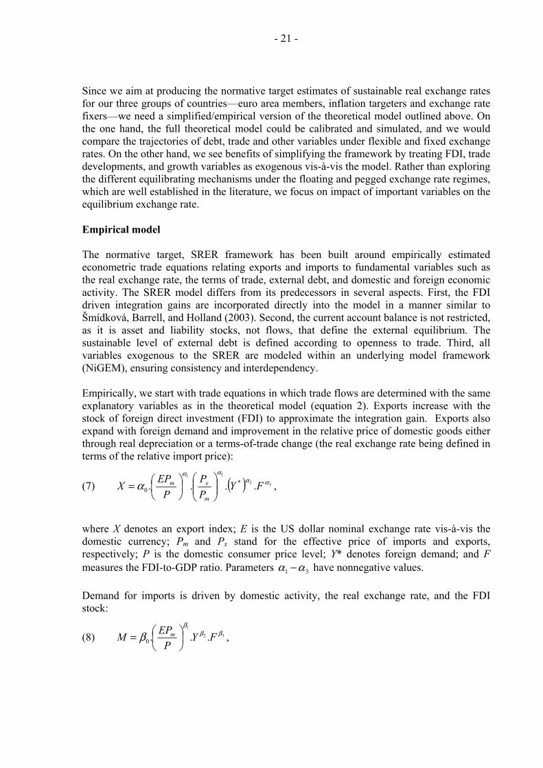
Since we aim at producing the normative target estimates of sustainable real exchange rates for our three groups of countries—euro area members, inflation targeters and exchange rate fixers—we need a simplified/empirical version of the theoretical model outlined above. On the one hand, the full theoretical model could be calibrated and simulated, and we would compare the trajectories of debt, trade and other variables under flexible and fixed exchange rates. On the other hand, we see benefits of simplifying the framework by treating FDI, trade developments, and growth variables as exogenous vis-à-vis the model. Rather than exploring the different equilibrating mechanisms under the floating and pegged exchange rate regimes, which are well established in the literature, we focus on impact of important variables on the equilibrium exchange rate. Empirical model The normative target, SRER framework has been built around empirically estimated econometric trade equations relating exports and imports to fundamental variables such as the real exchange rate, the terms of trade, external debt, and domestic and foreign economic activity. The SRER model differs from its predecessors in several aspects. First, the FDI driven integration gains are incorporated directly into the model in a manner similar to Šmídková, Barrell, and Holland (2003). Second, the current account balance is not restricted, as it is asset and liability stocks, not flows, that define the external equilibrium. The sustainable level of external debt is defined according to openness to trade. Third, all variables exogenous to the SRER are modeled within an underlying model framework (NiGEM), ensuring consistency and interdependency. Empirically, we start with trade equations in which trade flows are determined with the same explanatory variables as in the theoretical model (equation 2). Exports increase with the stock of foreign direct investment (FDI) to approximate the integration gain. Exports also expand with foreign demand and improvement in the relative price of domestic goods either through real depreciation or a terms-of-trade change (the real exchange rate being defined in terms of the relative import price):

(7) ( ) 32

11

.... *0

αααα

α FYPP

PEPX

m

xm⎟⎟⎠

⎞⎜⎜⎝

⎛⎟⎠⎞

⎜⎝⎛= ,

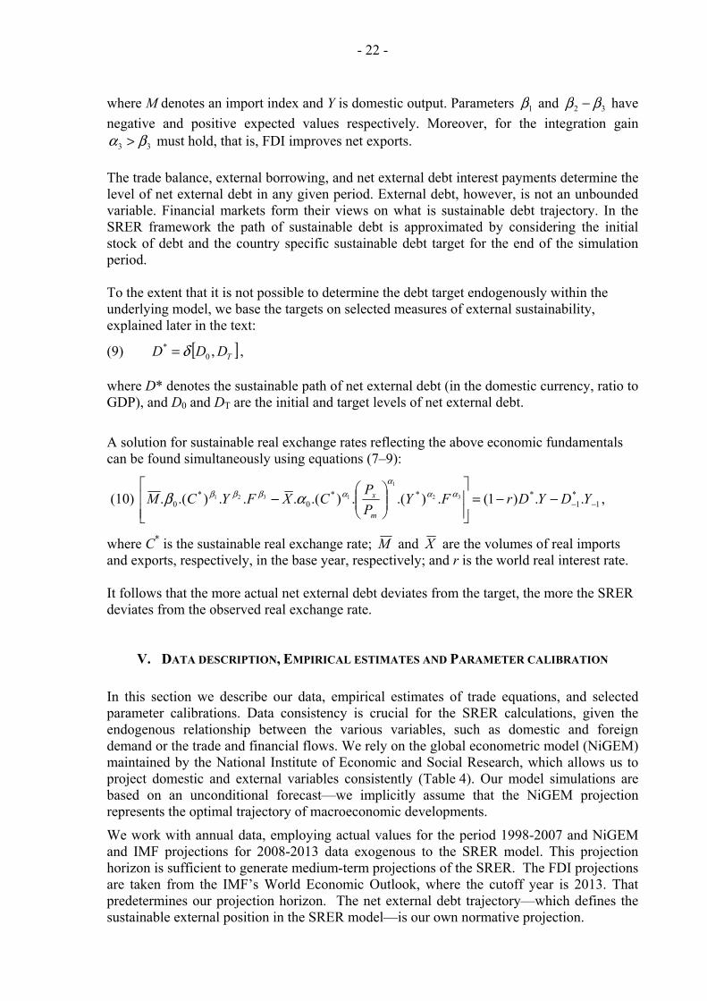
where X denotes an export index; E is the US dollar nominal exchange rate vis-à-vis the domestic currency; Pm and Px stand for the effective price of imports and exports, respectively; P is the domestic consumer price level; Y* denotes foreign demand; and F measures the FDI-to-GDP ratio. Parameters 31 αα − have nonnegative values. Demand for imports is driven by domestic activity, the real exchange rate, and the FDI stock:

(8) 32

1

...0ββ

β

β FYP

EPM m ⎟⎠⎞

⎜⎝⎛= ,

- 22 -

here M denotes an import index and Y is domestic output. Parameters w 1β and 32 ββ − have negative and positive expected values respectively. Moreover, for the integration gain

33 βα > must hold, that is, FDI improves net exports. The trade balance, external borrowing, and net external debt interest payments determine the level of net external debt in any given period. External debt, however, is not an unbounded

ariablev . Financial markets form their views on what is sustainable debt trajectory. In the itial tion

he extent that it is n t possible to determine the debt target endogenously within the underlying model, we base the targets on selected measures of external sustainability,

o of net external debt.

tion for sustainable real exchange rates reflecting the above economic fundamentals

can be found simultaneously using equations (7–9):

SRER framework the path of sustainable debt is approximated by considering the instock of debt and the country specific sustainable debt target for the end of the simulaperiod. To t o

explained later in the text:

(9) [ ]DDD ,* δ= , T0

where D* denotes the sustainable path of net external debt (in the domestic currency, ratio tGDP), and D0 and DT are the initial and target levels

A solu

(10) 1*1

***0

*0 ..)1(.).(.).(...).(. 32

1

1321−−−−=

⎥⎥⎤

⎢⎢⎡

⎟⎟⎠

⎜⎜⎝

⎛− YDYDrFY

PPCXFYCM x αααβββ αβ ,

⎦⎣

⎞

m

α

where C* is the sustainable real exchange rate; M X and are the volumes of real imports nd exports, respectively, in the base year, respectively; and a r is the world real interest rate.

ER

rch, which allows us to

jections are taken from the IMF’s World Economic Outlook, where the cutoff year is 2013. That predetermines our projection horizon. The net external debt trajectory—which defines the sustainable external position in the SRER model—is our own normative projection.

It follows that the more actual net external debt deviates from the target, the more the SRdeviates from the observed real exchange rate.

V. DATA DESCRIPTION, EMPIRICAL ESTIMATES AND PARAMETER CALIBRATION

In this section we describe our data, empirical estimates of trade equations, and selected parameter calibrations. Data consistency is crucial for the SRER calculations, given the endogenous relationship between the various variables, such as domestic and foreign demand or the trade and financial flows. We rely on the global econometric model (NiGEM) maintained by the National Institute of Economic and Social Reseaproject domestic and external variables consistently (Table 4). Our model simulations are based on an unconditional forecast—we implicitly assume that the NiGEM projection represents the optimal trajectory of macroeconomic developments.

We work with annual data, employing actual values for the period 1998-2007 and NiGEM and IMF projections for 2008-2013 data exogenous to the SRER model. This projection horizon is sufficient to generate medium-term projections of the SRER. The FDI pro

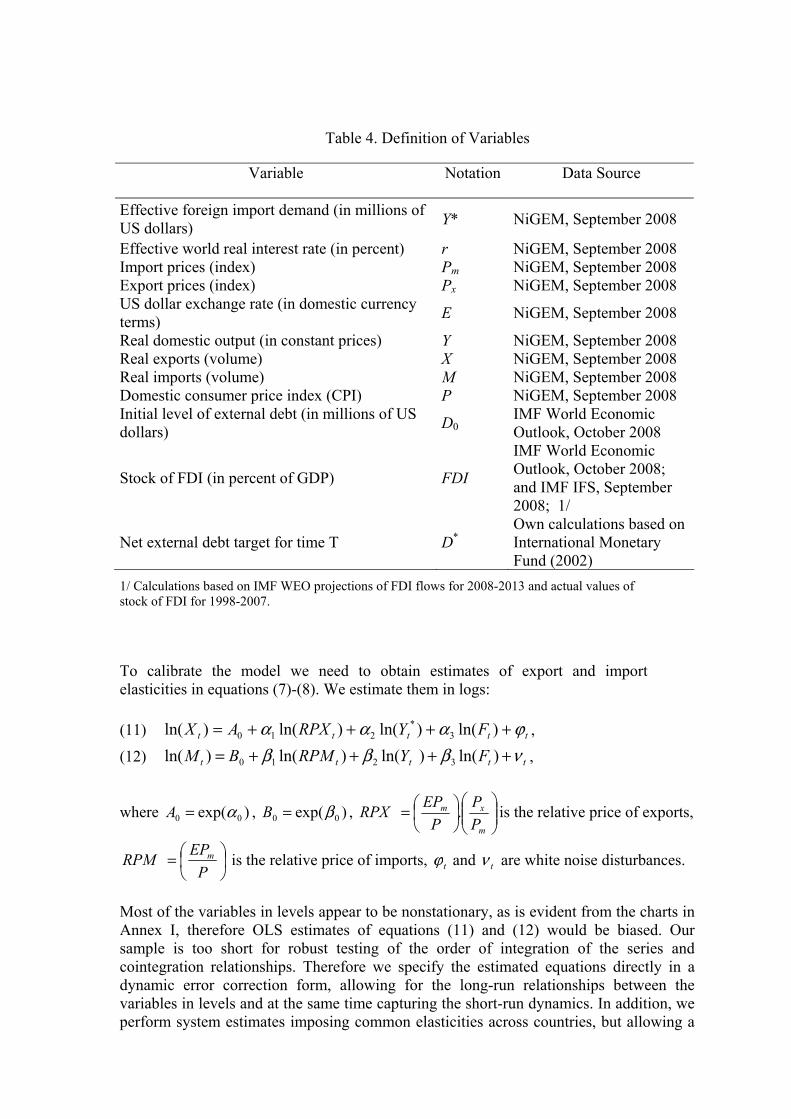
Table 4. Definition of Variables

Variable Notation Data Source

Effective foreign import demand (in millions of US dollars) Y* NiGEM, September 2008

Effective world real interest rate (in percent) r NiGEM, September 2008 Import prices (index) Pm NiGEM, September 2008 Export prices (index) Px NiGEM, September 2008 US dollar exchange rate (in domestic currency terms) E NiGEM, September 2008

Real domestic output (in constant prices) Y NiGEM, September 2008 Real exports (volume) X NiGEM, September 2008 Real imports (volume) M NiGEM, September 2008 Domestic consumer price index (CPI) P NiGEM, September 2008 Initial level of external debt (in millions of US dollars) D0

IMF World Economic Outlook, October 2008

Stock of FDI (in percent of GDP) FDI

IMF World Economic Outlook, October 2008; and IMF IFS, September 2008; 1/

Net external debt target for time T D* Own calculations based on International Monetary Fund (2002)

1/ Calculations based on IMF WEO projections of FDI flows for 2008-2013 and actual values of stock of FDI for 1998-2007.

To calibrate the model we need to obtain estimates of export and import elasticities in equations (7)-(8). We estimate them in logs: (11) , ttttt FYRPXAX ϕααα ++++= )ln()ln()ln()ln( 3

*210

(12) , ttttt FYRPMBM νβββ ++++= )ln()ln()ln()ln( 3210

where )exp( 00 α=A , )exp( 00 β=B , ⎟⎟⎠

⎞⎜⎜⎝

⎛⎟⎠⎞

⎜⎝⎛=

m

xm

PP

PEPRPX . is the relative price of exports,

⎟⎠⎞

⎜⎝⎛=

PEPRPM m is the relative price of imports, tϕ and tν are white noise disturbances.

Most of the variables in levels appear to be nonstationary, as is evident from the charts in Annex I, therefore OLS estimates of equations (11) and (12) would be biased. Our sample is too short for robust testing of the order of integration of the series and cointegration relationships. Therefore we specify the estimated equations directly in a dynamic error correction form, allowing for the long-run relationships between the variables in levels and at the same time capturing the short-run dynamics. In addition, we perform system estimates imposing common elasticities across countries, but allowing a

- 24 -

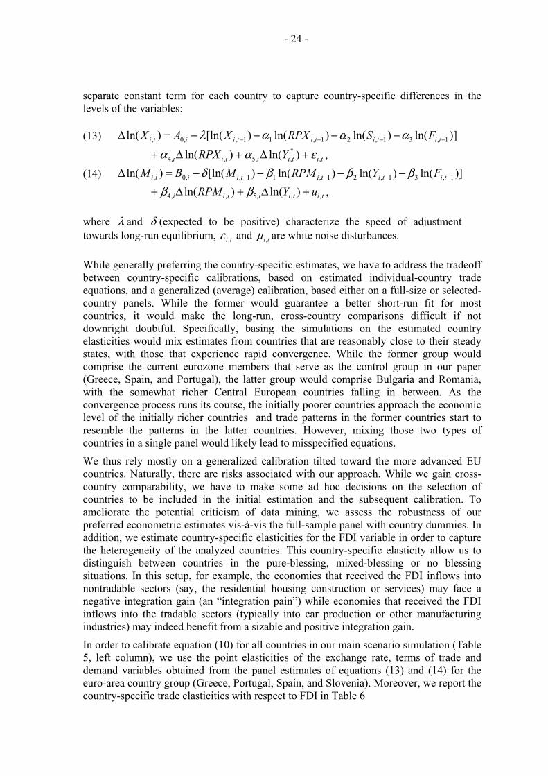
separate constant term for each country to capture country-specific differences in the levels of the variables: (13) )]ln()ln()ln()[ln()ln( 1,31,21,11,,0, −−−− −−−−=Δ titititiiti FSRPXXAX αααλ

, titiitii YRPX ,*,,5,,4 )ln()ln( εαα +Δ+Δ+

(14) )]ln()ln()ln()[ln()ln( 1,31,21,11,,0, −−−− −−−−=Δ titititiiti FYRPMMBM βββδ

titiitii uYRPM ,,,5,,4 )ln()ln( +Δ+Δ+ ββ , where λ and δ (expected to be positive) characterize the speed of adjustment towards long-run equilibrium, ti ,ε and ti ,μ are white noise disturbances. While generally preferring the country-specific estimates, we have to address the tradeoff between country-specific calibrations, based on estimated individual-country trade equations, and a generalized (average) calibration, based either on a full-size or selected-country panels. While the former would guarantee a better short-run fit for most countries, it would make the long-run, cross-country comparisons difficult if not downright doubtful. Specifically, basing the simulations on the estimated country elasticities would mix estimates from countries that are reasonably close to their steady states, with those that experience rapid convergence. While the former group would comprise the current eurozone members that serve as the control group in our paper (Greece, Spain, and Portugal), the latter group would comprise Bulgaria and Romania, with the somewhat richer Central European countries falling in between. As the convergence process runs its course, the initially poorer countries approach the economic level of the initially richer countries and trade patterns in the former countries start to resemble the patterns in the latter countries. However, mixing those two types of countries in a single panel would likely lead to misspecified equations.

We thus rely mostly on a generalized calibration tilted toward the more advanced EU countries. Naturally, there are risks associated with our approach. While we gain cross-country comparability, we have to make some ad hoc decisions on the selection of countries to be included in the initial estimation and the subsequent calibration. To ameliorate the potential criticism of data mining, we assess the robustness of our preferred econometric estimates vis-à-vis the full-sample panel with country dummies. In addition, we estimate country-specific elasticities for the FDI variable in order to capture the heterogeneity of the analyzed countries. This country-specific elasticity allow us to distinguish between countries in the pure-blessing, mixed-blessing or no blessing situations. In this setup, for example, the economies that received the FDI inflows into nontradable sectors (say, the residential housing construction or services) may face a negative integration gain (an “integration pain”) while economies that received the FDI inflows into the tradable sectors (typically into car production or other manufacturing industries) may indeed benefit from a sizable and positive integration gain.

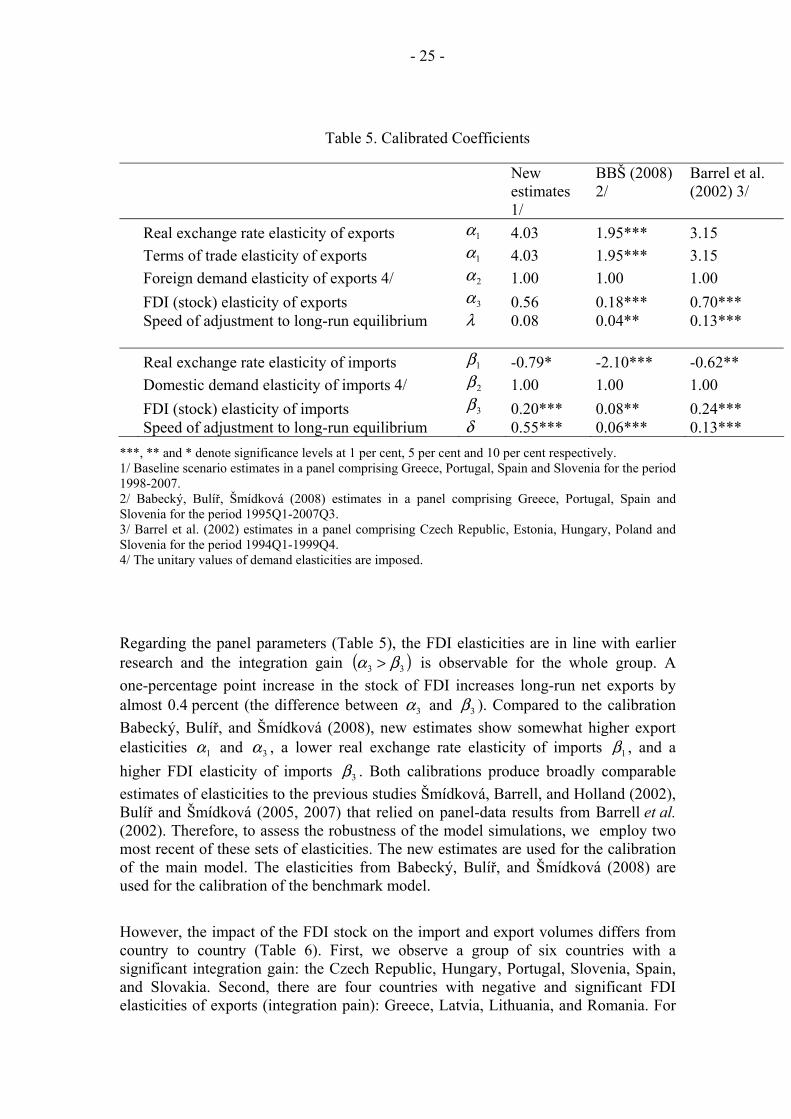
In order to calibrate equation (10) for all countries in our main scenario simulation (Table 5, left column), we use the point elasticities of the exchange rate, terms of trade and demand variables obtained from the panel estimates of equations (13) and (14) for the euro-area country group (Greece, Portugal, Spain, and Slovenia). Moreover, we report the country-specific trade elasticities with respect to FDI in Table 6

- 25 -

Table 5. Calibrated Coefficients

New estimates 1/

BBŠ (2008) 2/

Barrel et al. (2002) 3/

Real exchange rate elasticity of exports 1α 4.03 1.95*** 3.15 Terms of trade elasticity of exports 1α 4.03 1.95*** 3.15 Foreign demand elasticity of exports 4/ 2α 1.00 1.00 1.00 FDI (stock) elasticity of exports 3α 0.56 0.18*** 0.70*** Speed of adjustment to long-run equilibrium λ 0.08 0.04** 0.13*** Real exchange rate elasticity of imports 1β -0.79* -2.10*** -0.62** Domestic demand elasticity of imports 4/ 2β 1.00 1.00 1.00 FDI (stock) elasticity of imports 3β 0.20*** 0.08** 0.24*** Speed of adjustment to long-run equilibrium δ 0.55*** 0.06*** 0.13***

***, ** and * denote significance levels at 1 per cent, 5 per cent and 10 per cent respectively. 1/ Baseline scenario estimates in a panel comprising Greece, Portugal, Spain and Slovenia for the period 1998-2007. 2/ Babecký, Bulíř, Šmídková (2008) estimates in a panel comprising Greece, Portugal, Spain and Slovenia for the period 1995Q1-2007Q3. 3/ Barrel et al. (2002) estimates in a panel comprising Czech Republic, Estonia, Hungary, Poland and Slovenia for the period 1994Q1-1999Q4. 4/ The unitary values of demand elasticities are imposed.

Regarding the panel parameters (Table 5), the FDI elasticities are in line with earlier research and the integration gain ( 33 )βα > is observable for the whole group. A one-percentage point increase in the stock of FDI increases long-run net exports by almost 0.4 percent (the difference between 3α and 3β ). Compared to the calibration Babecký, Bulíř, and Šmídková (2008), new estimates show somewhat higher export elasticities 1α and 3α , a lower real exchange rate elasticity of imports 1β , and a higher FDI elasticity of imports 3β . Both calibrations produce broadly comparable estimates of elasticities to the previous studies Šmídková, Barrell, and Holland (2002), Bulíř and Šmídková (2005, 2007) that relied on panel-data results from Barrell et al. (2002). Therefore, to assess the robustness of the model simulations, we employ two most recent of these sets of elasticities. The new estimates are used for the calibration of the main model. The elasticities from Babecký, Bulíř, and Šmídková (2008) are used for the calibration of the benchmark model.

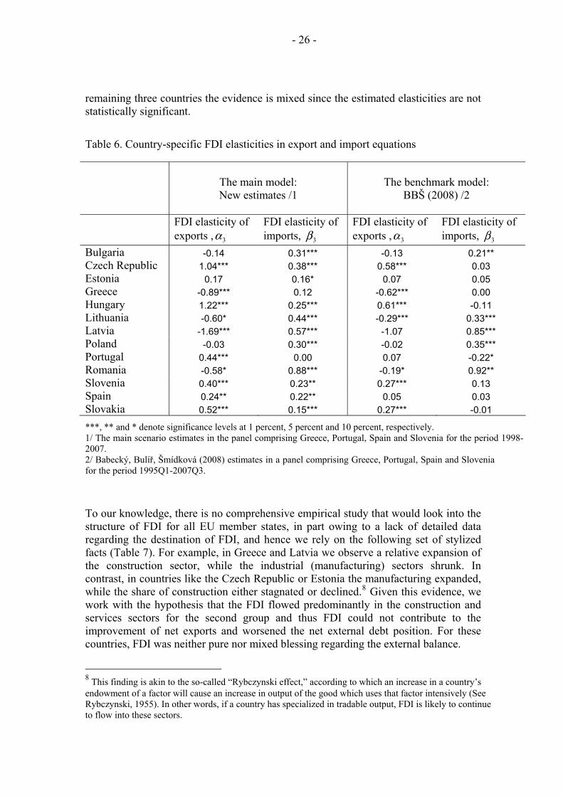
However, the impact of the FDI stock on the import and export volumes differs from country to country (Table 6). First, we observe a group of six countries with a significant integration gain: the Czech Republic, Hungary, Portugal, Slovenia, Spain, and Slovakia. Second, there are four countries with negative and significant FDI elasticities of exports (integration pain): Greece, Latvia, Lithuania, and Romania. For

- 26 -

remaining three countries the evidence is mixed since the estimated elasticities are not statistically significant.

Table 6. Country-specific FDI elasticities in export and import equations

The main model: New estimates /1

The benchmark model:

BBŠ (2008) /2

FDI elasticity of exports , 3α

FDI elasticity of imports, 3β

FDI elasticity of exports , 3α

FDI elasticity of imports, 3β

Bulgaria -0.14 0.31*** -0.13 0.21** Czech Republic 1.04*** 0.38*** 0.58*** 0.03 Estonia 0.17 0.16* 0.07 0.05 Greece -0.89*** 0.12 -0.62*** 0.00 Hungary 1.22*** 0.25*** 0.61*** -0.11 Lithuania -0.60* 0.44*** -0.29*** 0.33*** Latvia -1.69*** 0.57*** -1.07 0.85*** Poland -0.03 0.30*** -0.02 0.35*** Portugal 0.44*** 0.00 0.07 -0.22* Romania -0.58* 0.88*** -0.19* 0.92** Slovenia 0.40*** 0.23** 0.27*** 0.13 Spain 0.24** 0.22** 0.05 0.03 Slovakia 0.52*** 0.15*** 0.27*** -0.01

***, ** and * denote significance levels at 1 percent, 5 percent and 10 percent, respectively. 1/ The main scenario estimates in the panel comprising Greece, Portugal, Spain and Slovenia for the period 1998-2007. 2/ Babecký, Bulíř, Šmídková (2008) estimates in a panel comprising Greece, Portugal, Spain and Slovenia for the period 1995Q1-2007Q3.

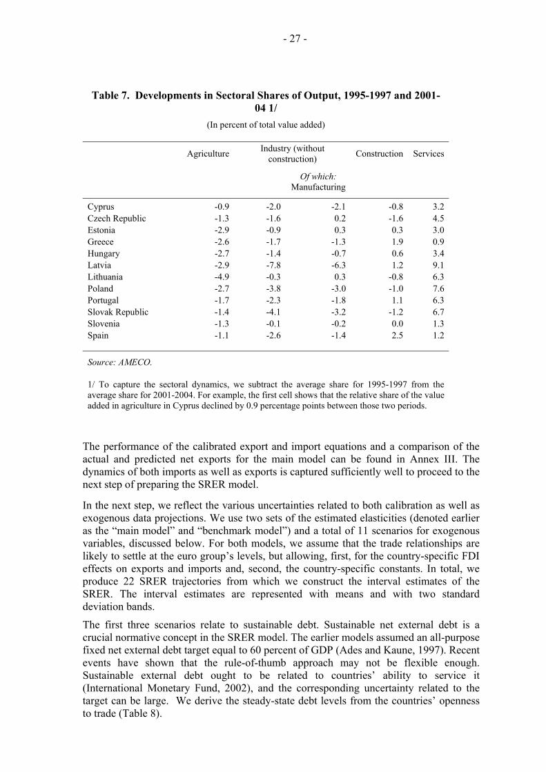
To our knowledge, there is no comprehensive empirical study that would look into the structure of FDI for all EU member states, in part owing to a lack of detailed data regarding the destination of FDI, and hence we rely on the following set of stylized facts (Table 7). For example, in Greece and Latvia we observe a relative expansion of the construction sector, while the industrial (manufacturing) sectors shrunk. In contrast, in countries like the Czech Republic or Estonia the manufacturing expanded, while the share of construction either stagnated or declined.8 Given this evidence, we work with the hypothesis that the FDI flowed predominantly in the construction and services sectors for the second group and thus FDI could not contribute to the improvement of net exports and worsened the net external debt position. For these countries, FDI was neither pure nor mixed blessing regarding the external balance.

8 This finding is akin to the so-called “Rybczynski effect,” according to which an increase in a country’s endowment of a factor will cause an increase in output of the good which uses that factor intensively (See Rybczynski, 1955). In other words, if a country has specialized in tradable output, FDI is likely to continue to flow into these sectors.

- 27 -

Table 7. Developments in Sectoral Shares of Output, 1995-1997 and 2001-04 1/

(In percent of total value added)

Agriculture Industry (without

construction) Construction Services

Of which:

Manufacturing

Cyprus -0.9 -2.0 -2.1 -0.8 3.2 Czech Republic -1.3 -1.6 0.2 -1.6 4.5 Estonia -2.9 -0.9 0.3 0.3 3.0 Greece -2.6 -1.7 -1.3 1.9 0.9 Hungary -2.7 -1.4 -0.7 0.6 3.4 Latvia -2.9 -7.8 -6.3 1.2 9.1 Lithuania -4.9 -0.3 0.3 -0.8 6.3 Poland -2.7 -3.8 -3.0 -1.0 7.6 Portugal -1.7 -2.3 -1.8 1.1 6.3 Slovak Republic -1.4 -4.1 -3.2 -1.2 6.7 Slovenia -1.3 -0.1 -0.2 0.0 1.3 Spain -1.1 -2.6 -1.4 2.5 1.2

Source: AMECO. 1/ To capture the sectoral dynamics, we subtract the average share for 1995-1997 from the average share for 2001-2004. For example, the first cell shows that the relative share of the value added in agriculture in Cyprus declined by 0.9 percentage points between those two periods.

The performance of the calibrated export and import equations and a comparison of the actual and predicted net exports for the main model can be found in Annex III. The dynamics of both imports as well as exports is captured sufficiently well to proceed to the next step of preparing the SRER model.

In the next step, we reflect the various uncertainties related to both calibration as well as exogenous data projections. We use two sets of the estimated elasticities (denoted earlier as the “main model” and “benchmark model”) and a total of 11 scenarios for exogenous variables, discussed below. For both models, we assume that the trade relationships are likely to settle at the euro group’s levels, but allowing, first, for the country-specific FDI effects on exports and imports and, second, the country-specific constants. In total, we produce 22 SRER trajectories from which we construct the interval estimates of the SRER. The interval estimates are represented with means and with two standard deviation bands.

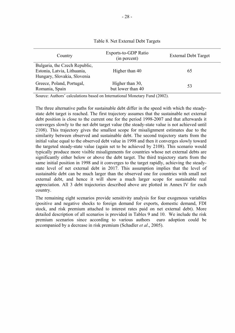
The first three scenarios relate to sustainable debt. Sustainable net external debt is a crucial normative concept in the SRER model. The earlier models assumed an all-purpose fixed net external debt target equal to 60 percent of GDP (Ades and Kaune, 1997). Recent events have shown that the rule-of-thumb approach may not be flexible enough. Sustainable external debt ought to be related to countries’ ability to service it (International Monetary Fund, 2002), and the corresponding uncertainty related to the target can be large. We derive the steady-state debt levels from the countries’ openness to trade (Table 8).

- 28 -

Table 8. Net External Debt Targets

Country Exports-to-GDP Ratio (in percent) External Debt Target

Bulgaria, the Czech Republic, Estonia, Latvia, Lithuania, Hungary, Slovakia, Slovenia

Higher than 40 65

Greece, Poland, Portugal, Romania, Spain

Higher than 30, but lower than 40 53

Source: Authors’ calculations based on International Monetary Fund (2002).

The three alternative paths for sustainable debt differ in the speed with which the steady-state debt target is reached. The first trajectory assumes that the sustainable net external debt position is close to the current one for the period 1998-2007 and that afterwards it converges slowly to the net debt target value (the steady-state value is not achieved until 2108). This trajectory gives the smallest scope for misalignment estimates due to the similarity between observed and sustainable debt. The second trajectory starts from the initial value equal to the observed debt value in 1998 and then it converges slowly toward the targeted steady-state value (again set to be achieved by 2108). This scenario would typically produce more visible misalignments for countries whose net external debts are significantly either below or above the debt target. The third trajectory starts from the same initial position in 1998 and it converges to the target rapidly, achieving the steady-state level of net external debt in 2017. This assumption implies that the level of sustainable debt can be much larger than the observed one for countries with small net external debt, and hence it will show a much larger scope for sustainable real appreciation. All 3 debt trajectories described above are plotted in Annex IV for each country.

The remaining eight scenarios provide sensitivity analysis for four exogenous variables (positive and negative shocks to foreign demand for exports, domestic demand, FDI stock, and risk premium attached to interest rates paid on net external debt). More detailed description of all scenarios is provided in Tables 9 and 10. We include the risk premium scenarios since according to various authors euro adoption could be accompanied by a decrease in risk premium (Schadler et al., 2005).

- 29 -

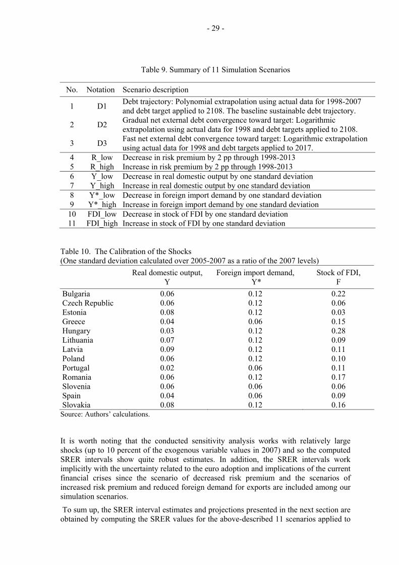
Table 9. Summary of 11 Simulation Scenarios

No. Notation Scenario description

1 D1 Debt trajectory: Polynomial extrapolation using actual data for 1998-2007 and debt target applied to 2108. The baseline sustainable debt trajectory.

2 D2 Gradual net external debt convergence toward target: Logarithmic extrapolation using actual data for 1998 and debt targets applied to 2108.

3 D3 Fast net external debt convergence toward target: Logarithmic extrapolation using actual data for 1998 and debt targets applied to 2017.

4 R_low Decrease in risk premium by 2 pp through 1998-2013 5 R_high Increase in risk premium by 2 pp through 1998-2013 6 Y_low Decrease in real domestic output by one standard deviation 7 Y_high Increase in real domestic output by one standard deviation 8 Y*_low Decrease in foreign import demand by one standard deviation 9 Y*_high Increase in foreign import demand by one standard deviation 10 FDI_low Decrease in stock of FDI by one standard deviation 11 FDI_high Increase in stock of FDI by one standard deviation

Table 10. The Calibration of the Shocks (One standard deviation calculated over 2005-2007 as a ratio of the 2007 levels)

Real domestic output,

Y Foreign import demand,

Y* Stock of FDI,

F Bulgaria 0.06 0.12 0.22 Czech Republic 0.06 0.12 0.06 Estonia 0.08 0.12 0.03 Greece 0.04 0.06 0.15 Hungary 0.03 0.12 0.28 Lithuania 0.07 0.12 0.09 Latvia 0.09 0.12 0.11 Poland 0.06 0.12 0.10 Portugal 0.02 0.06 0.11 Romania 0.06 0.12 0.17 Slovenia 0.06 0.06 0.06 Spain 0.04 0.06 0.09 Slovakia 0.08 0.12 0.16

Source: Authors’ calculations. It is worth noting that the conducted sensitivity analysis works with relatively large shocks (up to 10 percent of the exogenous variable values in 2007) and so the computed SRER intervals show quite robust estimates. In addition, the SRER intervals work implicitly with the uncertainty related to the euro adoption and implications of the current financial crises since the scenario of decreased risk premium and the scenarios of increased risk premium and reduced foreign demand for exports are included among our simulation scenarios.

To sum up, the SRER interval estimates and projections presented in the next section are obtained by computing the SRER values for the above-described 11 scenarios applied to

- 30 -

both model calibrations (main model and benchmark model). We suggest that this interval estimates should be robust to the most sensitive assumptions of our model.

VI. SIMULATION RESULTS

We report three types of simulation results (see Annex V for detailed results). First, for period 1999-2007 we report our indicator for the currency misalignment. Second, we show the SRER projections five years ahead. Third, we report the outcome of one selected scenario simulation—falling foreign demand—that is relevant for the current policy discussion in on the NMS in order to show the potential impact of the financial crisis on the SRER trajectories. Throughout the paper we use the EViews 6 (2007) package and the Gauss-Seidel simulation procedure with the solution period of 1998–2013. Exogenous variables are set equal to the observed values for the in-sample computations (1998–2007) and to the forecasted values for the out-of-sample computations (2008–2013).

Misalignment The misalignment indicator is based on the simulation results from the above-described 22 scenarios, pointing toward real exchange rate overvaluation/undervaluation if the interval is above/below the zero horizontal line. In the case of overvaluation/undervaluation the estimated sustainable real exchange rate is weaker/stronger than the observed one, even after considering various uncertainties related to the model calibration, exogenous variable projections, and normative definition of the debt target.

While most currencies seem to be close to the sustainable level, we identify at least one example of sizable misalignment in every group. Our simulations for the inflation targeting group identify at end-2007 only one country with a significantly overvalued currency (Romania), two countries with a marginally undervalued currencies (Hungary and Poland),9 and two countries without visible currency misalignment (the Czech Republic and Slovakia). Among the hard-peggers, we find three countries with an overvalued currency (Bulgaria, Latvia, and Lithuania) and one country without currency misalignment (Estonia). In the control group of the euro area members, there are three countries without significant currency misalignment (Slovenia, Spain, and Portugal) and one country with an overvalued currency (Greece). Consistent with the often mentioned external trade developments in Spain and Portugal, our simulations indicate that both countries went through a prolonged period of overvaluation following the euro adoption.

From these results we conclude that the current misalignment of currencies may not be a serious problem for the IT group of countries, with the exception of Romania that is anyway a latecomer to inflation targeting. It is also not a problem for the euro area group, with the exception of Greece. The group of hard-peggers, with the exception of Estonia,

9 In both cases the upper band of the misalignment corridor is touching the zero horizontal line, thus suggesting that the domestic currency was not misaligned under some scenarios.

- 31 -

is the group most likely to encounter problems in the year ahead stemming from the overvalued domestic currency.

The SRER projections

The SRER projections are computed for five years ahead in a similar fashion to the misalignment indicator, again relying on the interval indicator based on the 22 simulation scenarios. In our model, the countries with rapidly declining SRER trajectories, that is, sustainable appreciation, can withstand fast real exchange rate appreciation without endangering their development. On the one hand, appreciation is sustainable owing to a favorable set of fundamentals, such as the optimistic projection of FDI inflows, beneficial expected changes in terms of trade, or sustained increase in foreign demand for their exports. On the other hand, these countries may find themselves facing dilemma between the sustainable appreciation benefits and obstacles to the euro adoption. This dilemma refers to the mixed-blessing case of the FDI integration gain defined in the introduction.

Some countries may face only slowly declining or stable SRER trajectories and would not face any policy dilemma because mild sustainable real appreciation would be compatible with the nominal convergence required for the euro area entry. This scenario would be analogous to the pure-blessing case described in the introduction. Alternatively, some countries may face upward sloping SRER trajectories in the model, and hence they will have to deal with policy implications similar to those of the negative integration gain. These countries cannot afford the existing real exchange rate appreciation, because it is not sustainable. Moreover, the nominal convergence required for the euro adoption may not be a feasible option for them in the medium-term.

The SRER projections indicate that for the 2008-2013 period there are three countries (Czech Republic, Bulgaria, Romania) that may face the mixed-blessing type dilemma, because the estimated sustainable real appreciation is more than 2 percent per year annually. The estimates of the average sustainable real appreciation for the 2008-2013 period for the remaining euro candidates are around 1 percent only. This result suggests that the above-mentioned tradeoffs will be faced only by some of the NMS, specifically those who cumulated a large stocks of FDI and are at the same time faced with overall favorable conditions (such as a lower initial level of net external debt, growing external demand, and so on) or those who are in less advanced stages of convergence.

The projected sustainable real appreciation rates are significantly lower as compared to those estimated for the 1999-2007 period (Table 11). First, we observe a visible deceleration in the sustainable real appreciation for six countries (Czech Republic, Hungary, Portugal, Slovak Republic, Slovenia, Spain). While four of them are either in the euro area already or will join soon, the remaining two have yet to enter the ERM2 regime. We interpret this result as an argument that the mixed-blessing problem is not a long-term phenomena. In other words, its relevance is likely to fade away gradually as the convergence process advances further. Second, we identify four countries where the sustainable real appreciation is likely to accelerate (Bulgaria, Estonia, Lithuania, and Poland). Finally, for three countries (Greece, Latvia, and Romania) we observe that the SRERs switch from sustainable depreciation to sustainable appreciation. Countries in the last two groups, with the exception of Greece, are comparatively less advanced in their convergence process and hence may face the above-mentioned tradeoffs in the future.

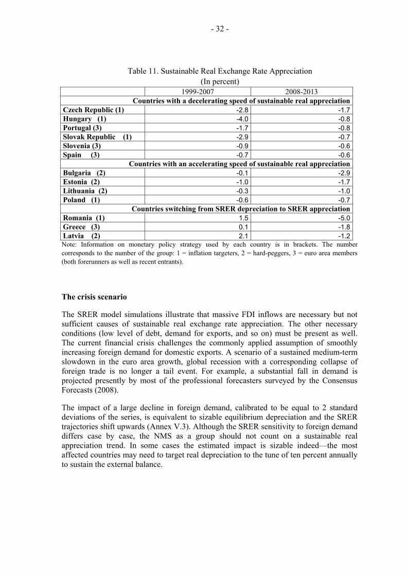
- 32 -

Table 11. Sustainable Real Exchange Rate Appreciation (In percent)

1999-2007 2008-2013 Countries with a decelerating speed of sustainable real appreciation

Czech Republic (1) -2.8 -1.7Hungary (1) -4.0 -0.8Portugal (3) -1.7 -0.8Slovak Republic (1) -2.9 -0.7Slovenia (3) -0.9 -0.6Spain (3) -0.7 -0.6

Countries with an accelerating speed of sustainable real appreciationBulgaria (2) -0.1 -2.9Estonia (2) -1.0 -1.7Lithuania (2) -0.3 -1.0Poland (1) -0.6 -0.7

Countries switching from SRER depreciation to SRER appreciation Romania (1) 1.5 -5.0Greece (3) 0.1 -1.8Latvia (2) 2.1 -1.2Note: Information on monetary policy strategy used by each country is in brackets. The number corresponds to the number of the group: 1 = inflation targeters, 2 = hard-peggers, 3 = euro area members (both forerunners as well as recent entrants).

The crisis scenario

The SRER model simulations illustrate that massive FDI inflows are necessary but not sufficient causes of sustainable real exchange rate appreciation. The other necessary conditions (low level of debt, demand for exports, and so on) must be present as well. The current financial crisis challenges the commonly applied assumption of smoothly increasing foreign demand for domestic exports. A scenario of a sustained medium-term slowdown in the euro area growth, global recession with a corresponding collapse of foreign trade is no longer a tail event. For example, a substantial fall in demand is projected presently by most of the professional forecasters surveyed by the Consensus Forecasts (2008).

The impact of a large decline in foreign demand, calibrated to be equal to 2 standard deviations of the series, is equivalent to sizable equilibrium depreciation and the SRER trajectories shift upwards (Annex V.3). Although the SRER sensitivity to foreign demand differs case by case, the NMS as a group should not count on a sustainable real appreciation trend. In some cases the estimated impact is sizable indeed—the most affected countries may need to target real depreciation to the tune of ten percent annually to sustain the external balance.

- 33 -

VII. POLICY IMPLICATIONS

We asked whether FDI is a mixed blessing for the NMS and we think that it indeed is in many of them. The NMS try to reap the integration gain of massive FDI inflows and simultaneously prepare for the euro adoption. On the upside, the economic literature suggests that the macroeconomic performance may be boosted through the FDI’s positive impact on the trade balance (we call this effect the integration gain) if FDI-financed projects expand the output of either exportable goods or substitutes for foreign imports. On the downside, this integration gain, foreseen by the financial markets, is likely to be reflected in the sharp appreciation of the real exchange rate that is sustainable in the medium-term, owing to the integration gain. The NMS may have lessened their chances to fulfill the Maastricht criteria and to adopt the euro flawlessly and FDI can be indeed a mixed blessing for them.

Not everybody will have such dilemma, though. For some NMS that have experienced only mild integration gains FDI can be a pure blessing as the resulting moderate real appreciation may be just compatible with the Maastricht criteria. Finally, for countries that have received FDI inflows predominantly into nontradable goods and services sectors FDI can be no blessing at all. Such inflows may be associated with a deteriorating trade balance, and consequently, a sustainable path for economic development would require real depreciation. Of course, sustained equilibrium real depreciation is incompatible with the Maastricht criteria and may lessen the chances of the euro adoption even more than the sharp appreciation observed in the first group of countries.

Our results show that the NMS do not form a homogenous group as far as the interaction of the real exchange rates and FDI is concerned. We identify only three NMS that are not euro area members for which FDI has brought a significant integration gain: the Czech Republic, Hungary, and Slovakia. From these three countries, only the Czech Republic is likely to face the mixed blessing policy dilemma since the lack of other necessary factors for this dilemma, such as limited net external debt, seems to offset the integration gain for Hungary and Slovakia. Consequently, the projected sustainable real appreciation is mild for these two countries (Figure 6). On the other side of the spectrum, we identify three countries (Latvia, Lithuania, and Romania) for which FDI can be no blessing at all since these inflows seem to have had a deteriorating impact on their trade balances. The two Baltic countries have strongly overvalued currencies because they have accumulated sizable net external debt without much integration gain.

Medium term appreciation of domestic currencies is not the only roadblock to the euro adoption and the NMS have to assess the alignment of their currencies. Overvalued currencies are expected to contribute to external imbalances, including external debt accumulation. For example, we observe that a fast euro adoption process may not be advisable for Romania and Bulgaria as we project both fast, medium-term real appreciation of the national currencies and their current overvaluation.

On the one hand, a fast real exchange rate appreciation may be sustainable in the case of a strong integration gain and a favorable net external debt level. While such conditions would complicate the process of euro adoption, they would do so only in the medium term. On the other hand, a mild real exchange rate appreciation is not necessarily making the process of euro adoption more sustainable. Such appreciation may be associated with a strong overvaluation in the case of the integration loss and high net external debt. In the latter case, the process of euro

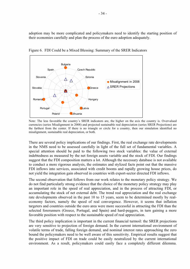
- 34 -

adoption may be more complicated and policymakers need to identify the starting position of their economies carefully and plan the process of the euro adoption adequately.

Figure 6. FDI Could be a Mixed Blessing: Summary of the SRER Indicators

Bulgaria

Czech Republic

Estonia

Greece

Hungary

Latvia

LithuaniaPoland

Portugal

Romania

Slovakia

Slovenia

Spain

Misalignment in 2008SRER Projections

Note: The less favorable the country´s SRER indicators are, the higher on the axis the country is. Overvalued currencies (series Misalignment in 2008) and projected sustainable real depreciation (series SRER Projections) are the farthest from the center. If there is no triangle or circle for a country, then our simulation identified no misalignment, sustainable real depreciation, or both.

There are several policy implications of our findings. First, the real exchange rate developments in the NMS need to be assessed carefully in light of the full set of fundamental variables. A special attention should be paid to the following two stock variables: the value of external indebtedness as measured by the net foreign assets variable and the stock of FDI. Our findings suggest that the FDI composition matters a lot. Although the necessary database is not available to conduct a more rigorous analysis, the estimates and stylized facts point out that the massive FDI inflows into services, associated with credit booms and rapidly growing house prices, do not yield the integration gain observed in countries with export-sector directed FDI inflows.

The second observation that follows from our work relates to the monetary policy strategy. We do not find particularly strong evidence that the choice of the monetary policy strategy may play an important role in the speed of real appreciation, and in the process of attracting FDI, or accumulating the stock of net external debt. The trend real appreciation and the real exchange rate developments observed in the past 10 to 15 years, seem to be determined mostly by real-economy factors, namely the speed of real convergence. However, it seems that inflation targeters and countries outside the euro area were more successful in attracting the FDI than the selected forerunners (Greece, Portugal, and Spain) and hard-peggers, in turn gaining a more favorable position with respect to the sustainable speed of real appreciation.

The third policy implication is important in the current financial turmoil: the SRER projections are very sensitive to projection of foreign demand. In the current international environment of volatile terms of trade, falling foreign demand, and nominal interest rates approaching the zero bound the policymakers need to be well aware of this sensitivity. Empirical results suggest that the positive impact of FDI on trade could be easily neutralized by the current international environment. As a result, policymakers could easily face a completely different dilemma.

- 35 -

Instead thinking about the mixed blessing of FDI, they could be faced with a need to depreciate real exchange rates in order to sustain the external balance.

The fourth issue worth considering for policy makers is the dynamics in the interaction between real exchange rates and the FDI. We have found some support—in this paper and in the relevant literature—for the standard hypotheses regarding the short, medium and long term impact of FDI. First, large foreign capital inflows, irrespective of their nature, tend to appreciate the domestic currency in the short run and/or increase the stock of international foreign exchange rate reserves. Second, FDI inflows, to the extent they stimulate either tradable output or import substitution, have also an appreciating impact on the real sustainable exchange rate that is our approximation of the external equilibrium. This impact is of medium-term nature, and – according to our estimates – is likely to diminish in the long-term when even the advanced stages of convergence are completed. Third, leaving aside the impact on the real equilibrium rate, a more volatile nominal rate in the short run imposes welfare costs of its own. We have certainly observed that countries with sizable and irregular FDI inflows decided to sterilize at least a part of these inflows.

The last policy implication comes from the experience of forerunners, the EU members that adopted euro prior to the EU enlargement and that were relatively close to the NMS and their convergence trajectory. Forerunners did not attract additional FDI after euro adoption. The NMS should keep this in mind and work under assumption that FDI inflows are medium-term rather than long-term phenomena. As a result of diminishing integration gain and rapidly cumulating stock of net external debt, the forerunners went through a prolonged period of overvaluation after euro adoption. This period seems to be over for Portugal and Spain, but not for Greece where FDI inflows were associated with credit and house price booms. The forerunners´ adjustment process to the overvalued currency might be worth analyzing specially for the hard-peggers among the NMS. Inflation targeters might be helped by nominal depreciation in the case they find themselves in a similar situation.

The forerunners experience also brings the attention to the fact that adoption of the euro affects the path of the real equilibrium exchange rate. For example, as we have seen the case in Greece, the post euro risk premium could be a fraction of that before joining the euro area. The Greek long government paper risk premium on long-term Greek government paper was some 500 basis points as compared to the EMU average in the mid 1990s, sharply dropping to about 100 basis points after the drachma was replaced with the euro. Correspondingly, the cost of servicing the existing of stock of debt held by both residents and nonresidents declined dramatically. To put this result differently, for NMS with high risk premia the eventual cost of misaligned currencies could be trivial compared to the immediate benefits of the eurozone membership (Ozkan, Sibert, and Sutherland, 2004; Bulíř and Hurník, 2006; Schadler and others et al., 2005).

- 36 -

REFERENCES

Abiad, Abdul, Daniel Leigh, and Ashoka Mody, 2007, “International Finance and Income Convergence: Europe is Different,” IMF Working Paper, WP/07/64 (Washington, DC: International Monetary Fund). Available via the Internet: http://www.imf.org/external/pubs/ft/wp/2007/wp0764.pdf.

Ades, Alberto, and Federico Kaune, 1997, “A New Measure of Current Account

Sustainability for Developing Countries,” Goldman-Sachs Emerging Markets Economic Research.

Alfaro, Laura, Areendam Chanda, Sebnem Kalemli-Ozcan, and Selin Sayek, 2004, “FDI

and Economic Growth: the Role of Local Financial Markets,” Journal of International Economics, Vol. 64, No. 1, pp. 89–112.

Aykut, Dilek, and Selin Sayek, 2007, “The Role of the Sectoral Composition of FDI on

Growth,” in Do Multinationals Feed Local Development and Growth? edited by Lucia Piscitello and Grazia D. Santangelo (Amsterdam: Elsevier).

Babecký, Jan, Aleš Bulíř, and Kateřina Šmídková, 2008, “Sustainable Real Exchange Rates

when Trade Winds Are Plentiful”, National Institute Economic Review, No. 204 (April), pp. 98–107.

Baldwin, Richard E., and Philippe Martin, 1999, “Two Waves of Globalisation:

Superficial Similarities, Fundamental Differences,” NBER Working Paper No. 6904. Available via the Internet: http://www.nber.org/papers/w6904.pdf.

Baltzer , Markus, Lorenzo Cappiello, Roberto A. De Santis, and Simone Manganelli,

2008 “Measuring Financial Integration in New EU Member States”, ECB Occasional Paper Series No 81.

Barrell, Ray, Dawn Holland, Zoltán M. Jakab, Mihály A. Kovács, Kateřina Šmídková,

Urmas Sepp, and Uroš Čufer, 2002, “An Econometric Macro-model of Transition: Policy Choices in the Pre-Accession Period,” in Proceedings of AMFET'2001 Conference – Modelling Economies in Transition, Krag (Poland), (Lodz: Absolwent).

Barry, Frank, 2000. “Convergence in not Automatic: Lessons from Ireland for Central

and Eastern Europe”, World Economy, Vol. 23, 10, pp. 1379–1394. Bevan, Alan A., and Saul Estrin, 2004, “The Determinants of Foreign Direct Investment

into European Transition Economies,” Journal of Comparative Economics, Vol. 32 (December), pp. 775–787.

Blanchard, Olivier J., 1981, “Output, the Stock Market, and Interest Rates,” American

Economic Review, Vol. 71, No. 1 (March), pp. 132–143.

- 37 -

Borensztein, Eduardo, Jose De Gregorio, and Jong-Wha Lee, 1998, “How Does Foreign Direct Investment Affect Economic Growth?” Journal of International Economics, Vol. 45, No. 1, pp. 115–35.

Borio, Claudio and Andrew Filardo, 2006, “Globalisation and inflation: New cross-country evidence on the global determinants of domestic inflation, BIS. Bulíř, Aleš, and Jaromír Hurník, 2006, “The Maastricht Inflation Criterion: How

Unpleasant Is Purgatory?” Economic Systems, Volume 30, No. 4, pp. 385–404. Bulíř, Aleš, and Kateřina Šmídková, 2007, “Fast Sailing Toward the Euro: Dangers of the

Lee Shore” in Batini, N. (ed.) Monetary Policy in Emerging Markets and Other Developing Countries, New York, Nova Science Publishers, pp. 67–92.

Bulíř, Aleš, and Kateřina Šmídková, 2005, “Sustainable Real Exchange Rates in the New

Accession Countries: What Have We Learned from the Forerunners?” Economic Systems, Vol. 29, No. 2, pp. 163–186.

Bun, Maurice J.G., and Franc J.G.M. Klaasen, 2002, “Has the Euro Increased Trade?”

Tinbergen Institute Discussion Paper, TI 2002-108/2 (Amsterdam: Tinbergen Institute). Available via the Internet: http://www.tinbergen.nl/discussionpapers/02108.pdf.

Campos, Nauro F., and Yuko Kinoshika, 2003, “Why Does FDI Go Where It Goes? New

Evidence from the Transition Economies,” IMF Working Paper, WP/03/228 (Washington, DC: International Monetary Fund). Available via the Internet: http://www.imf.org/external/pubs/cat/longres.cfm?sk=16954.0.

Carare, Alina, and Mark R. Stone, 2003, “Inflation Targeting Regimes,” IMF Working

Paper No. 03/9 (Washington, DC: International Monetary Fund). Available via the internet: http://www.imf.org/external/pubs/ft/wp/2003/wp0309.pdf.

Cincibuch, Martin, and Jiří Podpiera, 2004, “Beyond Balassa-Samuelson: Real

Appreciation in Tradables in Transition Countries,” CNB Working Paper No. 9 (Prague: Czech National Bank.). Available via the Internet: http://www.cnb.cz/en/pdf/CNBWP92004.pdf.

Čihák, Martin and Tomáš Holub, 2005, " Price Convergence in EU-Accession Countries: Evidence from the International Comparison ," Economie Internationale, No. 102, Issue 2, pp. 59-82, 2005 . Consensus Forecasts, 2008, Eastern Europe Consensus Forecasts and G-7 & Western

Europe. Consensus Economics, December 2008. http://www.consensuseconomics.com/

Égert, Balász, 2002, “Estimating the Impact of the Balassa–Samuelson Effect on Inflation

and the Real Exchange Rate During the Transition,” Economic Systems, Vol. 26, pp. 1–16.

- 38 -

EViews, 2007, Version 6, A computer package for estimations and model simulations. http://www.eviews.com/

Frankel, Jeffrey and Andrew Rose, 2002, “An Estimate Of The Effect Of Common

Currencies On Trade And Income,” Quarterly Journal of Economics, Vol. 117(2), pp. 437–466.

Driver, Rebecca, and Peter F. Westaway, 2005, “Concepts of Equilibrium Exchange Rates,” Bank of England Working Paper No. 247 (London: Bank of England). Available via the Internet: http://www.bankofengland.co.uk/workingpapers/wp247.pdf.

Giannone, Domenico, Michele Lenza, and Lucrezia Reichlin, 2008, “Explaining the

Great Moderation: It Is not the Shocks,” ECB Working Paper 865 (Frankfurt: European Central Bank). Available via the Internet: http://www.ecb.int/pub/pdf/scpwps/ecbwp865.pdf.

Goldstein, Morris, and Nicholas R. Lardy, 2005, “China's role in the revived Bretton

Woods system: A Case of Mistaken Identity,” Institute for International Economics Working Paper, WP 05–2 (Washington, DC). Available via the Internet: http://www.petersoninstitute.org/publications/wp/wp05-2.pdf.

Halpern, Lászlo and Charles Wyplosz, 1997, “Equilibrium Exchange Rates in Transition

Economies,” IMF Staff Papers, Vol. 44 (December), pp. 430–461. Holland, Dawn and Nigel Pain, 1998, “The Diffusion of Innovations in Central and

Eastern Europe: A Study of the Determinants and Impact of Foreign Direct Investment,” National Institute of Economic and Social Research Discussion Paper, No. 137. http://www.niesr.ac.uk/pubs/dps/dp137.pdf

Hunya, Gábor, Mario Holzner, and Julia Wörz, 2007, “How to Assess the Impact of FDI

on an Economy,” OECD Concept Paper, http://www.oecd.org/dataoecd/9/0/38937107.pdf

International Monetary Fund, 2002, Assessing Sustainability, (Washington, DC:

International Monetary Fund). Available via the Internet: http://www.imf.org/external/np/pdr/sus/2002/eng/052802.htm.

__________, 2008, “The European Credit Cycle: Diverging Patterns,” in Europe

Regional Economic Outlook, Fall 2008. (Washington, DC: International Monetary Fund). Available via the Internet: http://www.imf.org/External/Pubs/FT/REO/2008/EUR/ENG/ereo1008.pdf.

__________, 2008, World Economic Outlook, October 2008 (Washington, DC:

International Monetary Fund). Available via the Internet: http://www.imf.org/external/pubs/ft/weo/2008/02/pdf/text.pdf.

Yuko Kinoshita, 2008, “Is Foreign Direct Investment a Panacea?” IMF Research

Bulletin, March. Available via the Internet:

- 39 -

http://www.imf.org/External/Pubs/FT/irb/2008/02/index.pdf. Kinoshita, Yuko, and Chia-Hui Liu, 2008, “On the Role of Absorptive Capacity: FDI

Matters to Growth,” William Davidson Institute Working Paper, No. 845. Available via the Internet: http://www.wdi.umich.edu/files/Publications/WorkingPapers/wp845.pdf.

Kose, M. Ayhan, Eswar Prasad, Kenneth Rogoff, and Shang-Jin Wei, 2006, “Financial

Globalization: A Reappraisal,” IMF Working Paper, WP/06/189 (Washington DC: International Monetary Fund). Available via the Internet: www.imf.org/external/pubs/ft/wp/2006/wp06189.pdf.

Lane, Phillip R., and Gian Maria Milesi-Ferretti, 2002, “External Wealth, the Trade

Balance, and the Real Exchange Rate,” European Economic Review, Vol. 46 (June), pp. 1049–1071.

Lansbury, Melanie, Nigel Pain, and Kateřina Šmídková, 1996, “Foreign Direct

Investment in Central Europe Since 1990: An Econometric Study,” National Institute Economic Review, No. 156 (May), pp. 104–114.

Lim, Ewe-Ghee, 2001, “Determinants of, and the Relation Between, Foreign Direct

Investment and Growth: A Summary of the Recent Literature,” IMF Working Paper, WP/01/175 (Washington, DC: International Monetary Fund). Available via the Internet: http://www.imf.org/external/pubs/cat/longres.cfm?sk=15435.0.

Mody, Ashoka, and Antu Panini Murshid, 2005, “Growing Up With Capital Flows,”

Journal of International Economics, Vol. 65, No. 1, pp. 249–66. National Institute Global Econometric Model (NiGEM), 2008, (London: The National

Institute of Economic and Social Research). Ozkan, Gulcin F., Anne Sibert, and Alan Sutherland, 2004, “Monetary Union and the

Maastricht inflation Criterion: The Accession Countries,” Economics of Transition, Vol. 12, No. 4, pp. 635–52.

Rybczynski, Tadeus M., 1955, “Factor Endowment and Relative Commodity Prices,”

Economica, Vol. 22, No. 87, pp.336–41. Schadler, Susan, Paulo Drummond, Louis Kuijs, Zuzana Murgasova, and Rachel van

Elkan, 2005, “Adopting the Euro in Central Europe—Challenges of the Next Step in European Integration,” IMF Occasional Paper, No. 234 (Washington DC: International Monetary Fund).

Stone, Mark R., 2003, “Inflation Targeting Lite,” IMF Working Paper, No. 03/12

(Washington DC: International Monetary Fund). Available via the internet: http://www.imf.org/external/pubs/ft/wp/2003/wp0312.pdf.

- 40 -

Sylwester, Kevin, 2005, “Foreign Direct Investment, Growth and Income Inequality in Less Developed Countries,” International Review of Applied Economics, 19(3), pp. 289–300.

Šmídková, Kateřina, Ray Barrell, and Dawn Holland, 2003, “Estimates of Fundamental Real Exchange Rates for the Five EU Pre-Accession Countries”, Prague Economic Papers, No. 4, pp. 291–318.

Šmídková, Kateřina, Ray Barrell, and Dawn Holland, 2002, “Estimates of FRERs for the

Five EU Accession Countries,” CNB Working Paper, No. 3 (Prague: Czech National Bank). Available via the Internet: http://www.cnb.cz/en/pdf/WP_3_2002.pdf.

Williamson, John, 1994, Estimating Equilibrium Exchange Rates, (Washington DC:

Institute for International Economics).

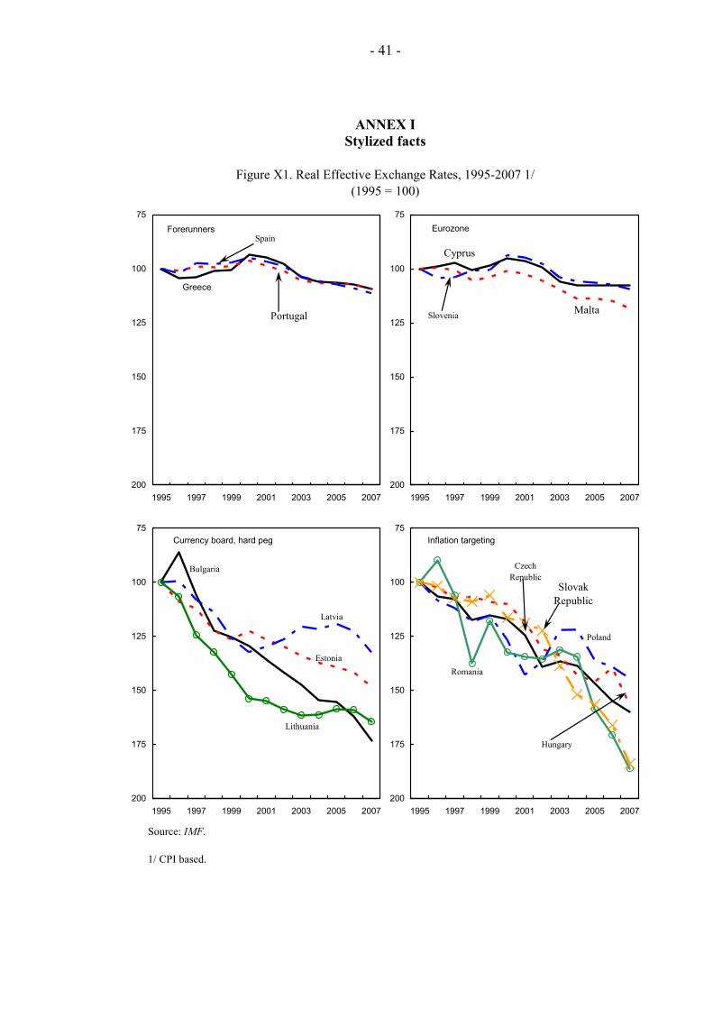
- 41 -

ANNEX I Stylized facts

Figure X1. Real Effective Exchange Rates, 1995-2007 1/

(1995 = 100)

Source: IMF.

1/ CPI based.

Forerunners

Greece

Portugal

Spain

75

100

125

150

175

2001995 1997 1999 2001 2003 2005 2007

Eurozone

Slovenia

Cyprus

Malta

75

100

125

150

175

2001995 1997 1999 2001 2003 2005 2007

Currency board, hard peg

Bulgaria

Estonia

Latvia

Lithuania

75

100

125

150

175

2001995 1997 1999 2001 2003 2005 2007

Inflation targeting

Czech Republic

Hungary

Poland

Romania

Slovak Republic

75

100

125

150

175

2001995 1997 1999 2001 2003 2005 2007

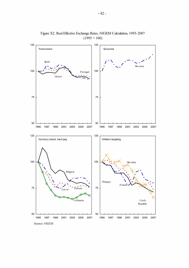
- 42 -

Figure X2. Real Effective Exchange Rates, NIGEM Calculation, 1995-2007(1995 = 100)

Source: NIGEM.

Forerunners

Greece

Portugal

Spain

50

75

100

125

1995 1997 1999 2001 2003 2005 2007

Eurozone

Slovenia

50

75

100

125

1995 1997 1999 2001 2003 2005 2007

Currency board, hard peg

Bulgaria

Estonia Latvia

Lithuania

50

75

100

125

1995 1997 1999 2001 2003 2005 2007

Inflation targeting

Czech Republic

Hungary Poland

Slovakia

50

75

100

125

1995 1997 1999 2001 2003 2005 2007

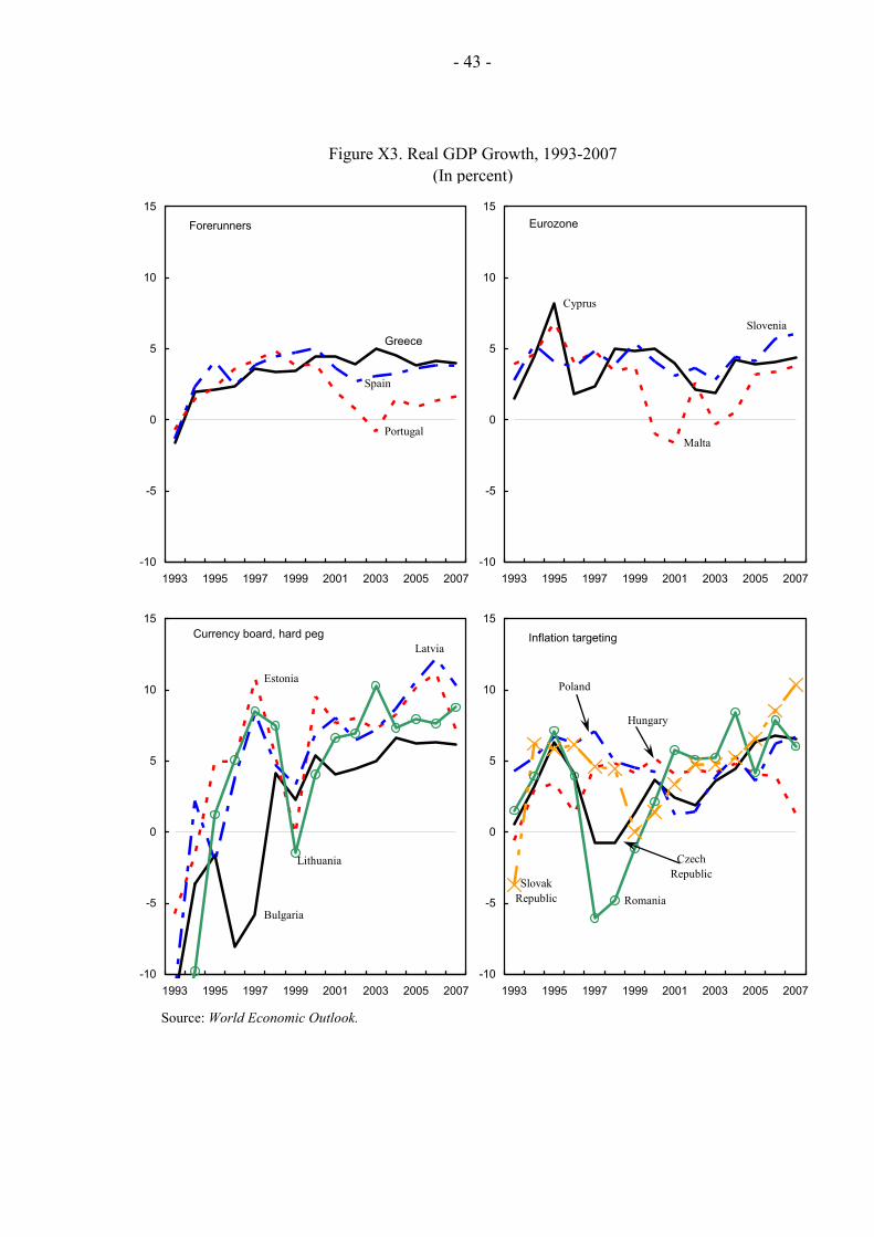
- 43 -

Figure X3. Real GDP Growth, 1993-2007(In percent)

Source: World Economic Outlook.

Forerunners

Greece

Portugal

Spain

-10

-5

0

5

10

15

1993 1995 1997 1999 2001 2003 2005 2007

Eurozone

Cyprus

Malta

Slovenia

-10

-5

0

5

10

15

1993 1995 1997 1999 2001 2003 2005 2007

Currency board, hard peg

Bulgaria

Estonia

Latvia

Lithuania

-10

-5

0

5

10

15

1993 1995 1997 1999 2001 2003 2005 2007

Inflation targeting

Czech Republic

Hungary

Poland

RomaniaSlovak

Republic

-10

-5

0

5

10

15

1993 1995 1997 1999 2001 2003 2005 2007

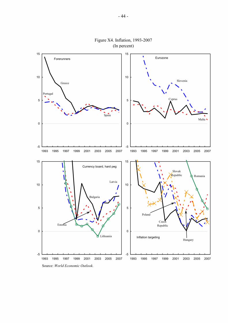
- 44 -

Figure X4. Inflation, 1993-2007(In percent)

Source: World Economic Outlook.

Forerunners

Greece

Portugal

Spain

-5

0

5

10

15

1993 1995 1997 1999 2001 2003 2005 2007

Eurozone

Cyprus

Malta

Slovenia

-5

0

5

10

15

1993 1995 1997 1999 2001 2003 2005 2007

Currency board, hard peg

Bulgaria

Estonia

Latvia

Lithuania

-5

0

5

10

15

1993 1995 1997 1999 2001 2003 2005 2007

Inflation targeting

Czech Republic

Hungary

Poland

RomaniaSlovak

Republic

-5

0

5

10

15

1993 1995 1997 1999 2001 2003 2005 2007

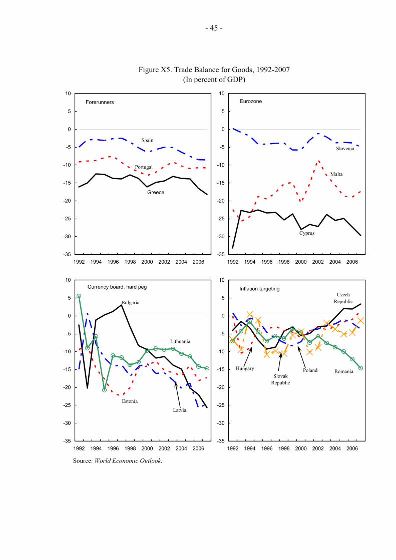
- 45 -

Figure X5. Trade Balance for Goods, 1992-2007(In percent of GDP)

Source: World Economic Outlook.

Forerunners

Greece

Portugal

Spain

-35

-30

-25

-20

-15

-10

-5

0

5

10

1992 1994 1996 1998 2000 2002 2004 2006

Eurozone

Cyprus

Malta

Slovenia

-35

-30

-25

-20

-15

-10

-5

0

5

10

1992 1994 1996 1998 2000 2002 2004 2006

Currency board, hard peg

Bulgaria

Estonia

Latvia

Lithuania

-35

-30

-25

-20

-15

-10

-5

0

5

10

1992 1994 1996 1998 2000 2002 2004 2006

Inflation targetingCzech

Republic

Hungary Poland RomaniaSlovak

Republic

-35

-30

-25

-20

-15

-10

-5

0

5

10

1992 1994 1996 1998 2000 2002 2004 2006

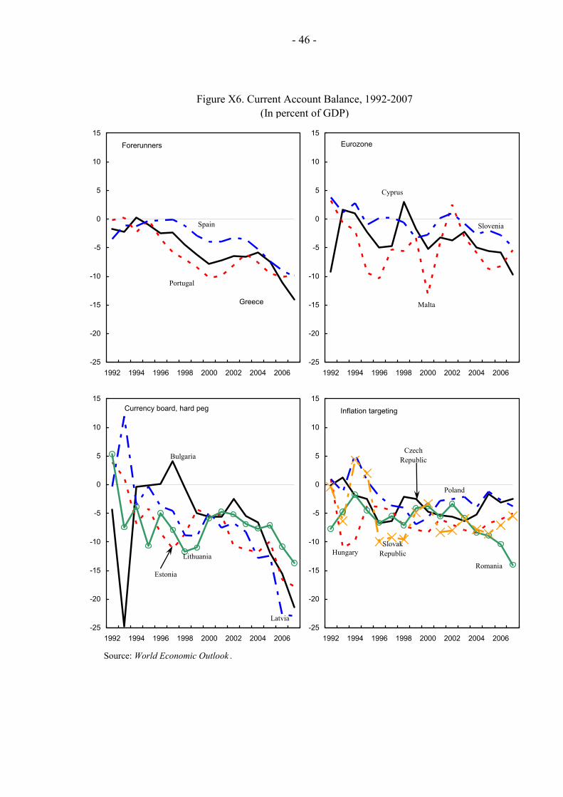
- 46 -

Figure X6. Current Account Balance, 1992-2007(In percent of GDP)

Source: World Economic Outlook .

Forerunners

Greece

Portugal

Spain

-25

-20

-15

-10

-5

0

5

10

15

1992 1994 1996 1998 2000 2002 2004 2006

Eurozone

Cyprus

Malta

Slovenia

-25

-20

-15

-10

-5

0

5

10

15

1992 1994 1996 1998 2000 2002 2004 2006

Currency board, hard peg

Bulgaria

Estonia

Latvia

Lithuania

-25

-20

-15

-10

-5

0

5

10

15

1992 1994 1996 1998 2000 2002 2004 2006

Inflation targeting

Czech Republic

Hungary

Poland

Romania

Slovak Republic

-25

-20

-15

-10

-5

0

5

10

15

1992 1994 1996 1998 2000 2002 2004 2006

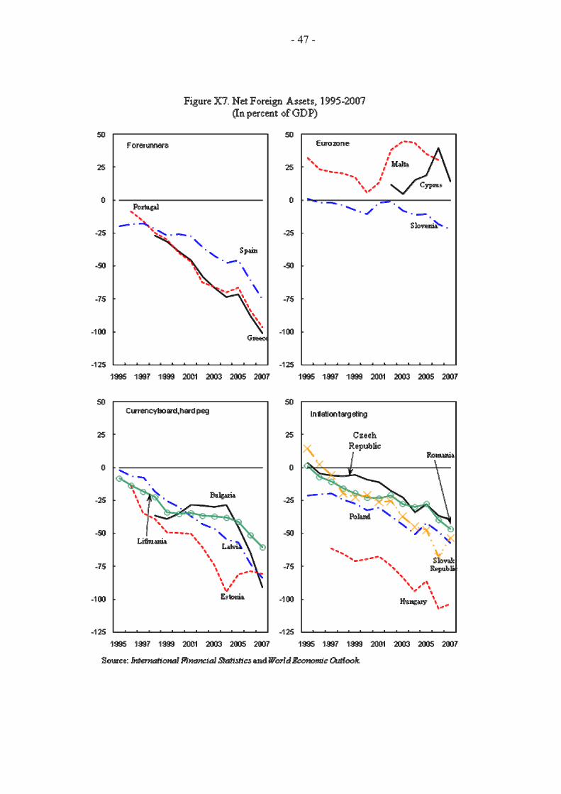
- 47 -

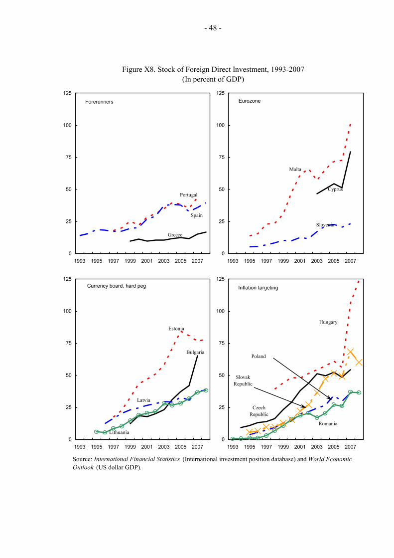
- 48 -

Figure X8. Stock of Foreign Direct Investment, 1993-2007(In percent of GDP)

Source: International Financial Statistics (International investment position database) and World Economic Outlook (US dollar GDP).

Forerunners

Greece

Portugal

Spain

0

25

50

75

100

125

1993 1995 1997 1999 2001 2003 2005 2007

Eurozone

Cyprus

Malta

Slovenia

0

25

50

75

100

125

1993 1995 1997 1999 2001 2003 2005 2007

Currency board, hard peg

Bulgaria

Estonia

Latvia

Lithuania 0

25

50

75

100

125

1993 1995 1997 1999 2001 2003 2005 2007

Inflation targeting

Czech Republic

Hungary

Poland

Romania

Slovak Republic

0

25

50

75

100

125

1993 1995 1997 1999 2001 2003 2005 2007

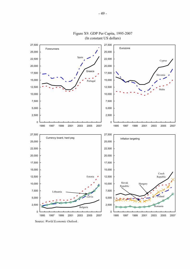
- 49 -

Figure X9. GDP Per Capita, 1995-2007(In constant US dollars)

Source: World Economic Outlook .

Forerunners

Greece

Portugal

Spain

0

2,500

5,000

7,500

10,000

12,500

15,000

17,500

20,000

22,500

25,000

27,500

1995 1997 1999 2001 2003 2005 2007

Eurozone

Cyprus

Malta

Slovenia

0

2,500

5,000

7,500

10,000

12,500

15,000

17,500

20,000

22,500

25,000

27,500

1995 1997 1999 2001 2003 2005 2007

Currency board, hard peg

Bulgaria

Estonia

Latvia

Lithuania

0

2,500

5,000

7,500

10,000

12,500

15,000

17,500

20,000

22,500

25,000

27,500

1995 1997 1999 2001 2003 2005 2007

Inflation targeting

Czech Republic

Hungary

Poland

Romania

Slovak Republic

0

2,500

5,000

7,500

10,000

12,500

15,000

17,500

20,000

22,500

25,000

27,500

1995 1997 1999 2001 2003 2005 2007

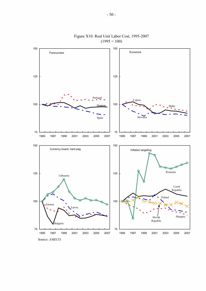
- 50 -

Figure X10. Real Unit Labor Cost, 1995-2007(1995 = 100)

Source: AMECO.

Forerunners

Greece

Portugal

Spain

75

100

125

150

1995 1997 1999 2001 2003 2005 2007

Eurozone

Cyprus

Malta

Slovenia

75

100

125

150

1995 1997 1999 2001 2003 2005 2007

Currency board, hard peg

Bulgaria

Estonia Latvia

Lithuania

75

100

125

150

1995 1997 1999 2001 2003 2005 2007

Inflation targeting

Czech Republic

Hungary

Poland

Romania

Slovak Republic

75

100

125

150

1995 1997 1999 2001 2003 2005 2007

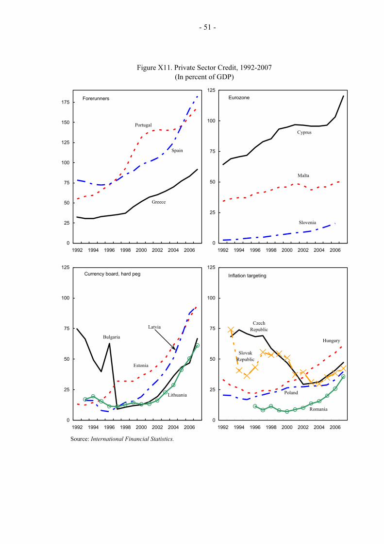
- 51 -

Figure X11. Private Sector Credit, 1992-2007(In percent of GDP)

Source: International Financial Statistics.

Forerunners

Greece

Portugal

Spain

0

25

50

75

100

125

150

175

1992 1994 1996 1998 2000 2002 2004 2006

Eurozone

Cyprus

Malta

Slovenia

0

25

50

75

100

125

1992 1994 1996 1998 2000 2002 2004 2006

Currency board, hard peg

Bulgaria

Estonia

Latvia

Lithuania

0

25

50

75

100

125

1992 1994 1996 1998 2000 2002 2004 2006

Inflation targeting

Czech Republic

Hungary

Poland

Romania

Slovak Republic

0

25

50

75

100

125

1992 1994 1996 1998 2000 2002 2004 2006

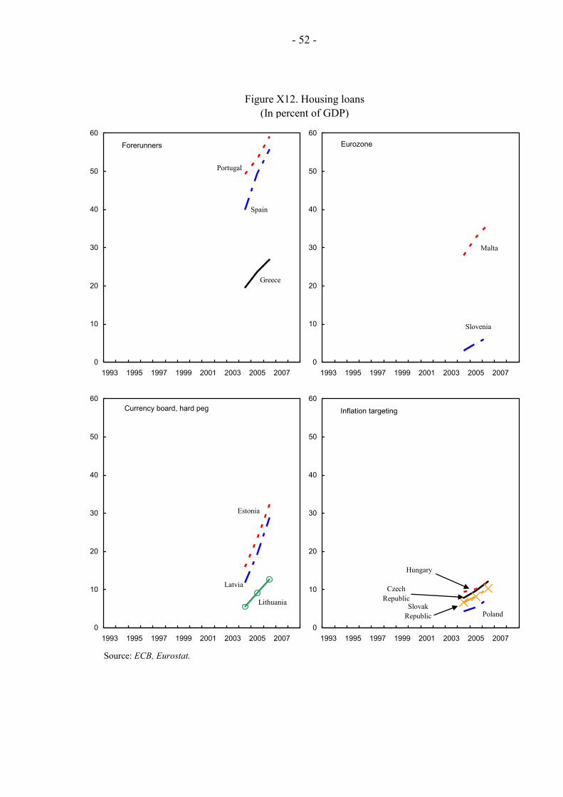
- 52 -

Figure X12. Housing loans(In percent of GDP)

Source: ECB, Eurostat.

Forerunners

Greece

Portugal

Spain

0

10

20

30

40

50

60

1993 1995 1997 1999 2001 2003 2005 2007

Eurozone

Malta

Slovenia

0

10

20

30

40

50

60

1993 1995 1997 1999 2001 2003 2005 2007

Currency board, hard peg

Estonia

Latvia

Lithuania

0

10

20

30

40

50

60

1993 1995 1997 1999 2001 2003 2005 2007

Inflation targeting

Czech Republic

Hungary

Poland Slovak

Republic 0

10

20

30

40

50

60

1993 1995 1997 1999 2001 2003 2005 2007

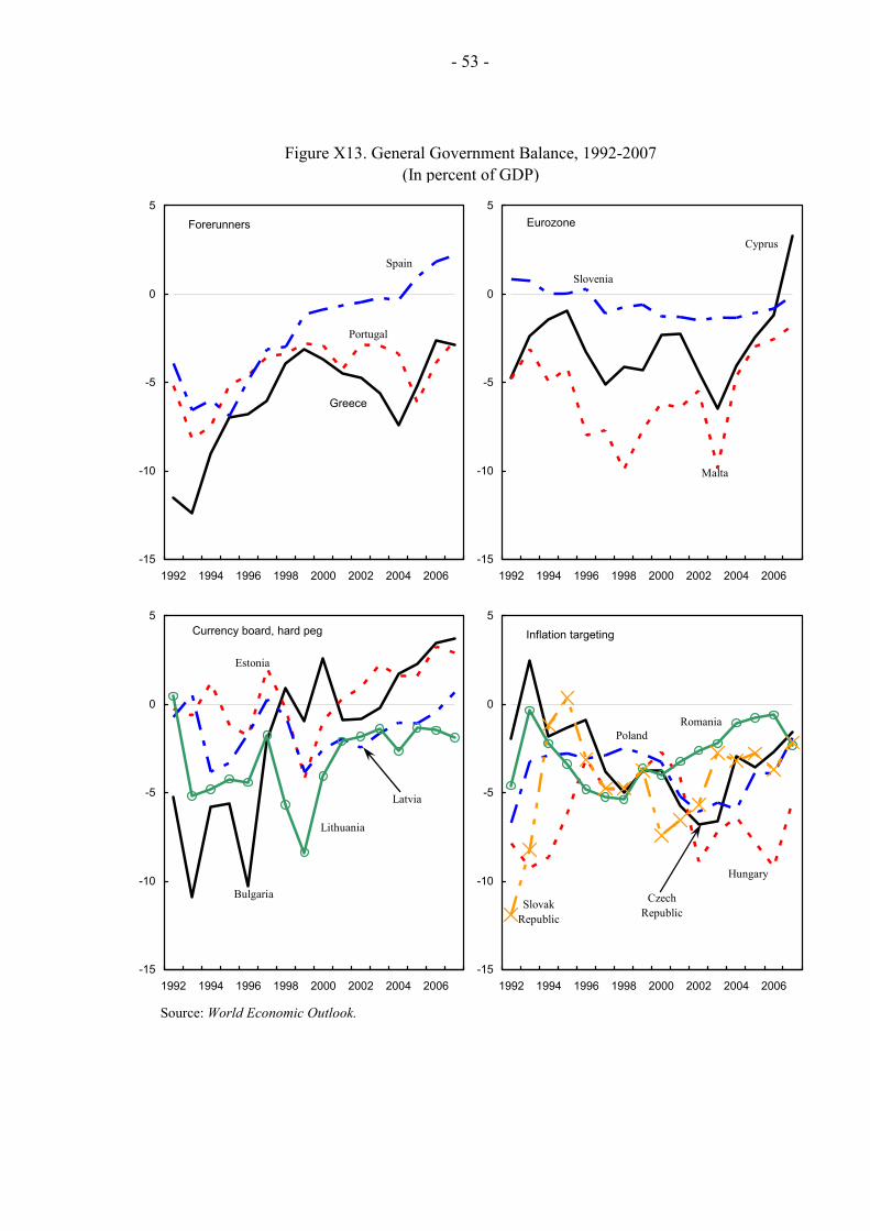
- 53 -

Figure X13. General Government Balance, 1992-2007(In percent of GDP)

Source: World Economic Outlook.

Forerunners

Greece

Portugal

Spain

-15

-10

-5

0

5

1992 1994 1996 1998 2000 2002 2004 2006

Eurozone

Cyprus

Malta

Slovenia

-15

-10

-5

0

5

1992 1994 1996 1998 2000 2002 2004 2006

Currency board, hard peg

Bulgaria

Estonia

Latvia

Lithuania

-15

-10

-5

0

5

1992 1994 1996 1998 2000 2002 2004 2006

Inflation targeting

Czech Republic

Hungary

Poland Romania

Slovak Republic

-15

-10

-5

0

5

1992 1994 1996 1998 2000 2002 2004 2006

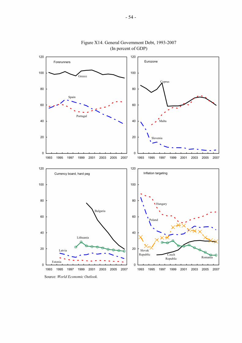
- 54 -

Figure X14. General Government Debt, 1993-2007(In percent of GDP)

Source: World Economic Outlook.

Forerunners

Greece

Portugal

Spain

0

20

40

60

80

100

120

1993 1995 1997 1999 2001 2003 2005 2007

Eurozone

Cyprus

Slovenia

Malta

0

20

40

60

80

100

120

1993 1995 1997 1999 2001 2003 2005 2007

Currency board, hard peg

Bulgaria

Estonia

Latvia

Lithuania

0

20

40

60

80

100

120

1993 1995 1997 1999 2001 2003 2005 2007

Inflation targeting

Czech Republic

Hungary

Poland

Romania

Slovak Republic

0

20

40

60

80

100

120

1993 1995 1997 1999 2001 2003 2005 2007

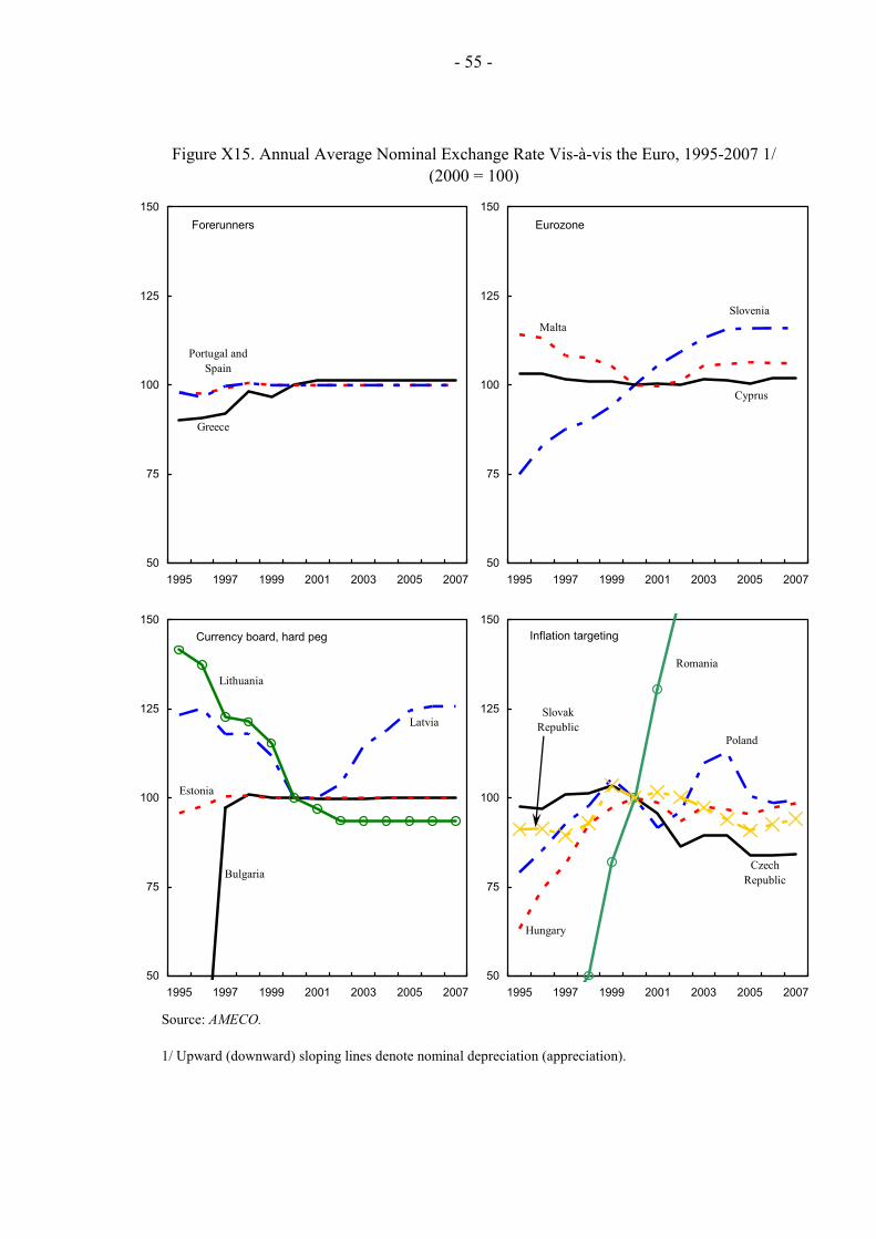
- 55 -

Figure X15. Annual Average Nominal Exchange Rate Vis-à-vis the Euro, 1995-2007 1/(2000 = 100)

Source: AMECO.

1/ Upward (downward) sloping lines denote nominal depreciation (appreciation).

Forerunners

Greece

Portugal and Spain

50

75

100

125

150

1995 1997 1999 2001 2003 2005 2007

Eurozone

Slovenia

Cyprus

Malta

50

75

100

125

150

1995 1997 1999 2001 2003 2005 2007

Currency board, hard peg

Bulgaria

Estonia

Latvia

Lithuania

50

75

100

125

150

1995 1997 1999 2001 2003 2005 2007

Inflation targeting

Czech Republic

Hungary

Poland

Slovak Republic

50

75

100

125

150

1995 1997 1999 2001 2003 2005 2007

Romania

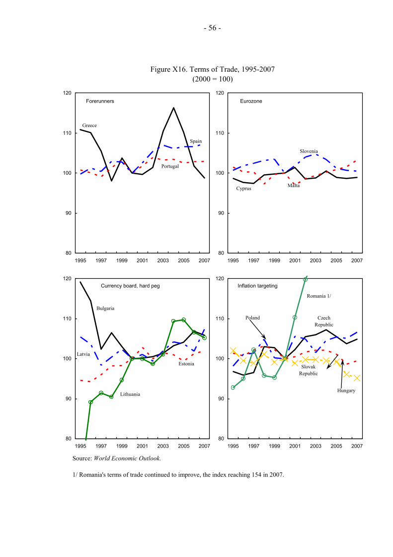
- 56 -

Figure X16. Terms of Trade, 1995-2007(2000 = 100)

Source: World Economic Outlook.

1/ Romania's terms of trade continued to improve, the index reaching 154 in 2007.

Forerunners

Greece

Portugal

Spain

80

90

100

110

120

1995 1997 1999 2001 2003 2005 2007

Eurozone

Slovenia

Cyprus Malta

80

90

100

110

120

1995 1997 1999 2001 2003 2005 2007

Currency board, hard peg

Bulgaria

Estonia

Latvia

Lithuania

80

90

100

110

120

1995 1997 1999 2001 2003 2005 2007

Inflation targeting

Czech Republic

Hungary

Poland

Slovak Republic

80

90

100

110

120

1995 1997 1999 2001 2003 2005 2007

Romania 1/

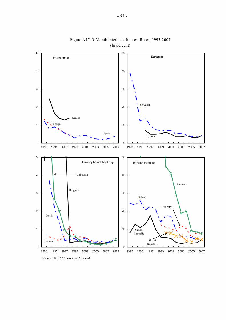
- 57 -

Figure X17. 3-Month Interbank Interest Rates, 1993-2007(In percent)

Source: World Economic Outlook.

Forerunners

Greece

Portugal

Spain

0

10

20

30

40

50

1993 1995 1997 1999 2001 2003 2005 2007

Eurozone

Cyprus

Slovenia

0

10

20

30

40

50

1993 1995 1997 1999 2001 2003 2005 2007

Currency board, hard peg

Bulgaria

Estonia

Latvia

Lithuania

0

10

20

30

40

50

1993 1995 1997 1999 2001 2003 2005 2007

Inflation targeting

Czech Republic

Hungary

Poland

Romania

Slovak Republic

0

10

20

30

40

50

1993 1995 1997 1999 2001 2003 2005 2007

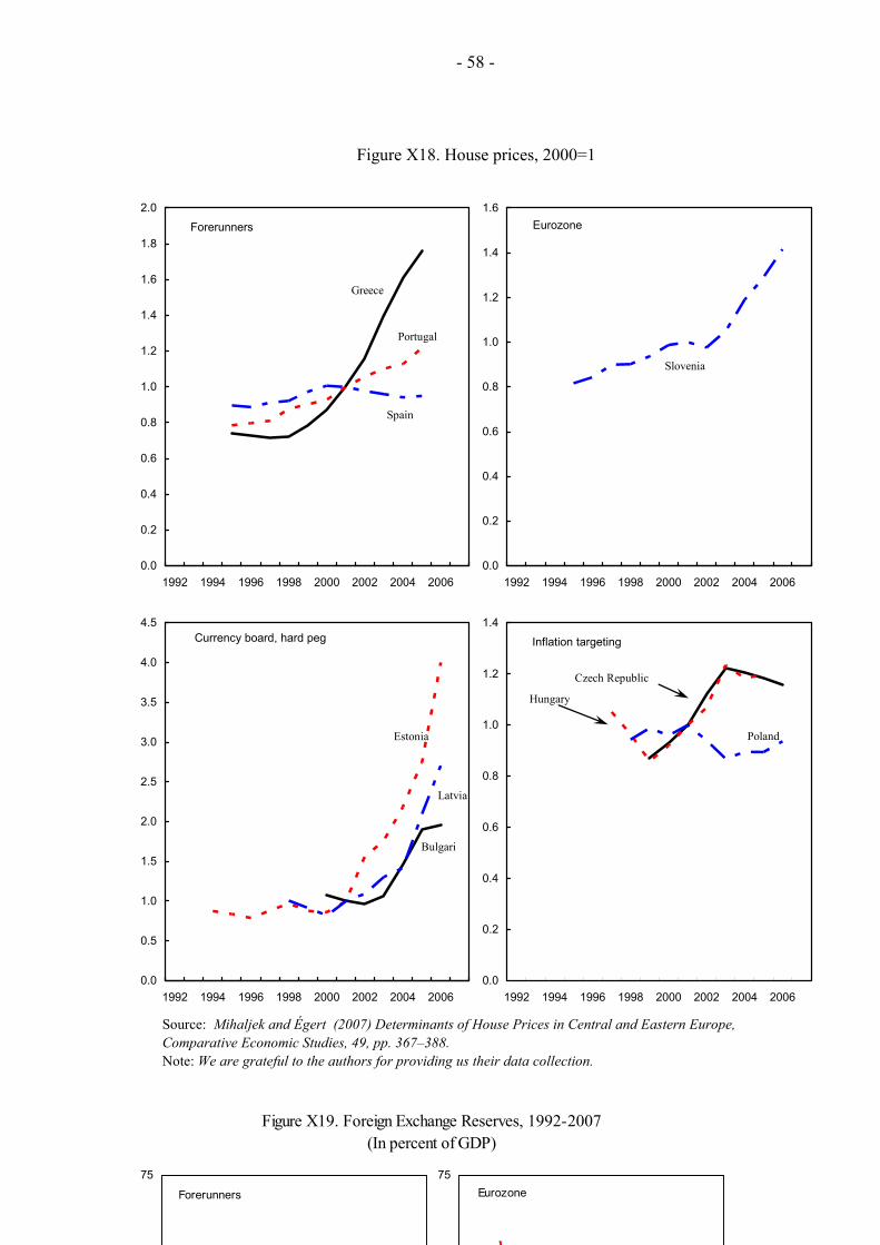
- 58 -

Figure X18. House prices, 2000=1

Source: Mihaljek and Égert (2007) Determinants of House Prices in Central and Eastern Europe, Comparative Economic Studies, 49, pp. 367–388.Note: We are grateful to the authors for providing us their data collection.

Forerunners

Greece

Portugal

Spain

0.0

0.2

0.4

0.6

0.8

1.0

1.2

1.4

1.6

1.8

2.0

1992 1994 1996 1998 2000 2002 2004 2006

Eurozone

Slovenia

0.0

0.2

0.4

0.6

0.8

1.0

1.2

1.4

1.6

1992 1994 1996 1998 2000 2002 2004 2006

Currency board, hard peg

Estonia

Latvia

0.0

0.5

1.0

1.5

2.0

2.5

3.0

3.5

4.0

4.5

1992 1994 1996 1998 2000 2002 2004 2006

Bulgari

Inflation targeting

Hungary

Poland

0.0

0.2

0.4

0.6

0.8

1.0

1.2

1.4

1992 1994 1996 1998 2000 2002 2004 2006

Czech Republic

Figure X19. Foreign Exchange Reserves, 1992-2007(In percent of GDP)

Eurozone75

Forerunners

75

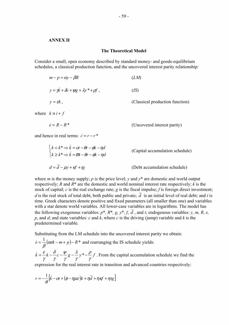
- 59 -

ANNEX II

The Theoretical Model Consider a small, open economy described by standard money- and goods-equilibrium schedules, a classical production function, and the uncovered interest parity relationship: Rypm βα −=− (LM) , (IS) fygcky ρλψδγ ++++= *&

ky ε= , (Classical production function) where fik +≡ (Uncovered interest parity) *RRe −=& and hence in real terms: *rrc −=&

(Capital accumulation schedule) ⎩⎨⎧

−−−=⇒≥−−−=⇒<

dkrtkkkdkrtkkk

ηφθϖηφθο

&

&

**

gfydd ικμ ++−= (Debt accumulation schedule) where m is the money supply; p is the price level; y and y* are domestic and world output respectively; R and R* are the domestic and world nominal interest rate respectively; k is the stock of capital; c is the real exchange rate; g is the fiscal impulse; f is foreign direct investment; d is the real stock of total debt, both public and private; d is an initial level of real debt; and t is time. Greek characters denote positive and fixed parameters (all smaller than one) and variables with a star denote world variables. All lower-case variables are in logarithms. The model has the following exogenous variables: p*, R*, g, y*, f, d , and t; endogenous variables: y, m, R, e, p, and d; and state variables: c and k, where c is the driving (jump) variable and k is the predetermined variable. Substituting from the LM schedule into the uncovered interest parity we obtain:

( ) *1 Rpmke −+−= αεβ

& and rearranging the IS schedule yields:

fygckkγρ

γλ

γψ

γδ

γε −−−−= *& . From the capital accumulation schedule we find the

expression for the real interest rate in transition and advanced countries respectively:

( )[ ]gfdktkr ηιηκηημεφοθ

+++−+−−= &1

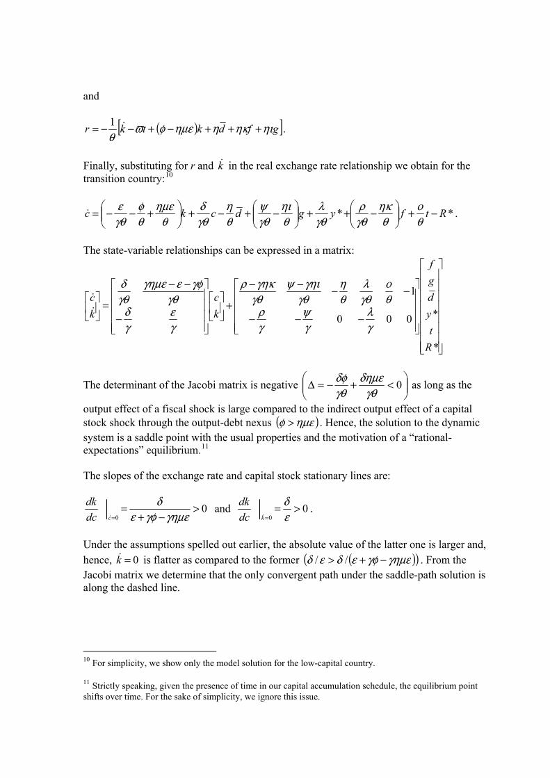
and

( )[ ]gfdktkr ηιηκηημεφϖθ

+++−+−−= &1 .

Finally, substituting for r and in the real exchange rate relationship we obtain for the transition country:

k&10

** Rtfygdckc −+⎟⎟⎠

⎞⎜⎜⎝

⎛ −++⎟⎟⎠

⎞⎜⎜⎝

⎛ −+−+⎟⎟⎠

⎞⎜⎜⎝

⎛ +−−=θο

θηκ

γθρ

γθλ

θηι

γθψ

θη

γθδ

θημε

θφ

γθε

& .

The state-variable relationships can be expressed in a matrix:

⎥⎥⎥⎥⎥⎥⎥⎥

⎦

⎤

⎢⎢⎢⎢⎢⎢⎢⎢

⎣

⎡

⎥⎥⎥⎥

⎦

⎤

⎢⎢⎢⎢

⎣

⎡

−−−

−−−−

+⎥⎦

⎤⎢⎣

⎡

⎥⎥⎥⎥

⎦

⎤

⎢⎢⎢⎢

⎣

⎡

−

−−

=⎥⎦

⎤⎢⎣

⎡

*

*000

1

Rt

ydgf

kc

kc

γλ

γψ

γρ

θο

γθλ

θη

γθγηιψ

γθγηκρ

γε

γδ

γθγφεγημε

γθδ

&&

The determinant of the Jacobi matrix is negative ⎟⎟⎠

⎞⎜⎜⎝

⎛ <+−=Δ 0γθ

δημεγθδφ as long as the

output effect of a fiscal shock is large compared to the indirect output effect of a capital stock shock through the output-debt nexus ( )ημεφ > . Hence, the solution to the dynamic system is a saddle point with the usual properties and the motivation of a “rational-expectations” equilibrium.11 The slopes of the exchange rate and capital stock stationary lines are:

00

>−+

== γημεγφε

δcdc

dk&

and 00

>== ε

δkdc

dk&

.

Under the assumptions spelled out earlier, the absolute value of the latter one is larger and, hence, is flatter as compared to the former 0=k& ( )( )γημεγφεδεδ −+> // . From the Jacobi matrix we determine that the only convergent path under the saddle-path solution is along the dashed line.

10 For simplicity, we show only the model solution for the low-capital country.

11 Strictly speaking, given the presence of time in our capital accumulation schedule, the equilibrium point shifts over time. For the sake of simplicity, we ignore this issue.

- 61 -

The schedule shifts as a result of the FDI, debt, and foreign demand shocks, respectively, as discussed in the text are:

00

<−=∂∂

= δργκη

cfc

& and 0

0<−=

∂∂

= δρ

kfc

&,

00

>=∂∂

= δγη

cdc

& and 0

0=

∂∂

=kdc

&, and

0** 00

<−=∂∂=

∂∂

== δλ

kc yc

yc

&&.

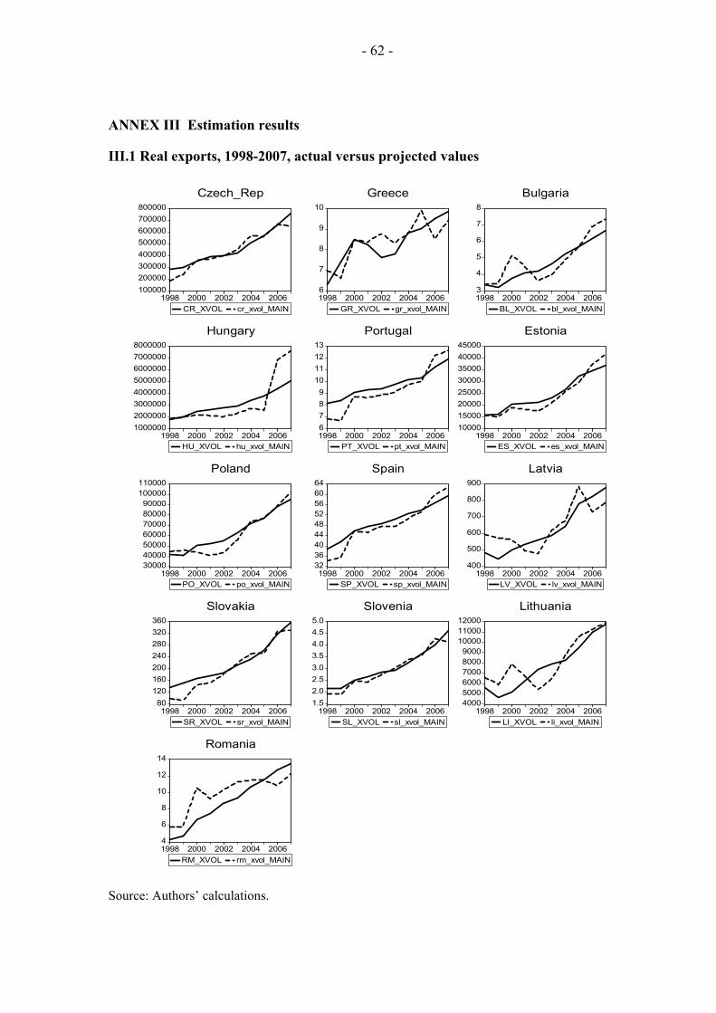
- 62 -

ANNEX III Estimation results

III.1 Real exports, 1998-2007, actual versus projected values

100000200000300000400000500000600000700000800000

1998 2000 2002 2004 2006CR_XVOL cr_xvol_MAIN

Czech_Rep

6

7

8

9

10

1998 2000 2002 2004 2006GR_XVOL gr_xvol_MAIN

Greece

3

4

5

6

7

8

1998 2000 2002 2004 2006BL_XVOL bl_xvol_MAIN

Bulgaria

10000002000000300000040000005000000600000070000008000000

1998 2000 2002 2004 2006HU_XVOL hu_xvol_MAIN

Hungary

6789

10111213

1998 2000 2002 2004 2006PT_XVOL pt_xvol_MAIN

Portugal

1000015000200002500030000350004000045000

1998 2000 2002 2004 2006ES_XVOL es_xvol_MAIN

Estonia

30000400005000060000700008000090000

100000110000

1998 2000 2002 2004 2006PO_XVOL po_xvol_MAIN

Poland

323640444852566064

1998 2000 2002 2004 2006SP_XVOL sp_xvol_MAIN

Spain

400

500

600

700

800

900

1998 2000 2002 2004 2006LV_XVOL lv_xvol_MAIN

Latvia

80120160200240280320360

1998 2000 2002 2004 2006SR_XVOL sr_xvol_MAIN

Slovakia

1.52.02.53.03.54.04.55.0

1998 2000 2002 2004 2006SL_XVOL sl_xvol_MAIN

Slovenia

400050006000700080009000

100001100012000

1998 2000 2002 2004 2006LI_XVOL li_xvol_MAIN

Lithuania

4

6

8

10

12

14

1998 2000 2002 2004 2006RM_XVOL rm_xvol_MAIN

Romania

Source: Authors’ calculations.

- 63 -

Actual values show export volumes (XVOL). Projected values (xvol_MAIN) are based on the main model that uses the new estimates of demand and price elasticities, country-specific FDI elasticities calibrated on 1998-2007 and constant terms calibrated on 2003-2007.

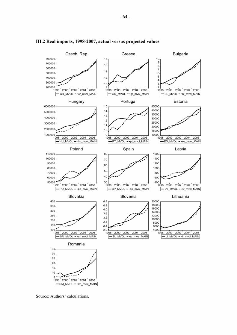
- 64 -

III.2 Real imports, 1998-2007, actual versus projected values

200000

300000

400000

500000

600000

700000

800000

1998 2000 2002 2004 2006CR_MVOL cr_mvol_MAIN

Czech_Rep

910

12

14

16

18

1998 2000 2002 2004 2006GR_MVOL gr_mvol_MAIN

Greece

23456789

10

1998 2000 2002 2004 2006BL_MVOL bl_mvol_MAIN

Bulgaria

1000000

2000000

3000000

4000000

5000000

6000000

1998 2000 2002 2004 2006HU_MVOL hu_mvol_MAIN

Hungary

9

10

11

12

13

14

15

1998 2000 2002 2004 2006PT_MVOL pt_mvol_MAIN

Portugal

1000015000200002500030000350004000045000

1998 2000 2002 2004 2006ES_MVOL es_mvol_MAIN

Estonia

50000

60000

70000

80000

90000

100000

110000

1998 2000 2002 2004 2006PO_MVOL po_mvol_MAIN

Poland

30

40

50

60

70

80

1998 2000 2002 2004 2006SP_MVOL sp_mvol_MAIN

Spain

400

600

800

1000

1200

1400

1600

1998 2000 2002 2004 2006LV_MVOL lv_mvol_MAIN

Latvia

100

150

200

250

300

350

400

1998 2000 2002 2004 2006SR_MVOL sr_mvol_MAIN

Slovakia

2.02.42.83.23.64.04.44.8

1998 2000 2002 2004 2006SL_MVOL sl_mvol_MAIN

Slovenia

400060008000

100001200014000160001800020000

1998 2000 2002 2004 2006LI_MVOL li_mvol_MAIN

Lithuania

5

10

15

20

25

30

35

1998 2000 2002 2004 2006RM_MVOL rm_mvol_MAIN

Romania

Source: Authors’ calculations.

- 65 -

Actual values show export volumes (MVOL). Projected values (mvol_MAIN) are based on the main model that uses the new estimates of demand and price elasticities, country-specific FDI elasticities calibrated on 1998-2007 and constant terms calibrated on 2003-2007.

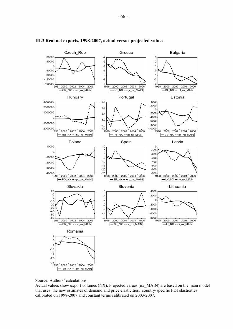
- 66 -

III.3 Real net exports, 1998-2007, actual versus projected values

-160000

-120000

-80000

-40000

0

40000

80000

1998 2000 2002 2004 2006CR_NX cr_nx_MAIN

Czech_Rep

-8

-7

-6

-5

-4

-3

-2

1998 2000 2002 2004 2006GR_NX gr_nx_MAIN

Greece

-3

-2

-1

0

1

2

3

1998 2000 2002 2004 2006BL_NX bl_nx_MAIN

Bulgaria

-2000000

-1000000

0

1000000

2000000

3000000

1998 2000 2002 2004 2006HU_NX hu_nx_MAIN

Hungary

-4.4-4.0

-3.2

-2.4

-1.6

-0.8

1998 2000 2002 2004 2006PT_NX pt_nx_MAIN

Portugal

-10000-8000-6000-4000-2000

020004000

1998 2000 2002 2004 2006ES_NX es_nx_MAIN

Estonia

-40000

-30000

-20000

-10000

0

10000

1998 2000 2002 2004 2006PO_NX po_nx_MAIN

Poland

-25-20-15-10-505

10

1998 2000 2002 2004 2006SP_NX sp_nx_MAIN

Spain

-700-600-500-400-300-200-100

0

1998 2000 2002 2004 2006LV_NX lv_nx_MAIN

Latvia

-60-50-40-30-20-10

01020

1998 2000 2002 2004 2006SR_NX sr_nx_MAIN

Slovakia

-.6

-.4

-.2

.0

.2

.4

.6

1998 2000 2002 2004 2006SL_NX sl_nx_MAIN

Slovenia

-8000

-6000

-4000

-2000

0

2000

4000

1998 2000 2002 2004 2006LI_NX li_nx_MAIN

Lithuania

-25

-20

-15

-10

-5

0

5

1998 2000 2002 2004 2006RM_NX rm_nx_MAIN

Romania

Source: Authors’ calculations. Actual values show export volumes (NX). Projected values (nx_MAIN) are based on the main model that uses the new estimates of demand and price elasticities, country-specific FDI elasticities calibrated on 1998-2007 and constant terms calibrated on 2003-2007.

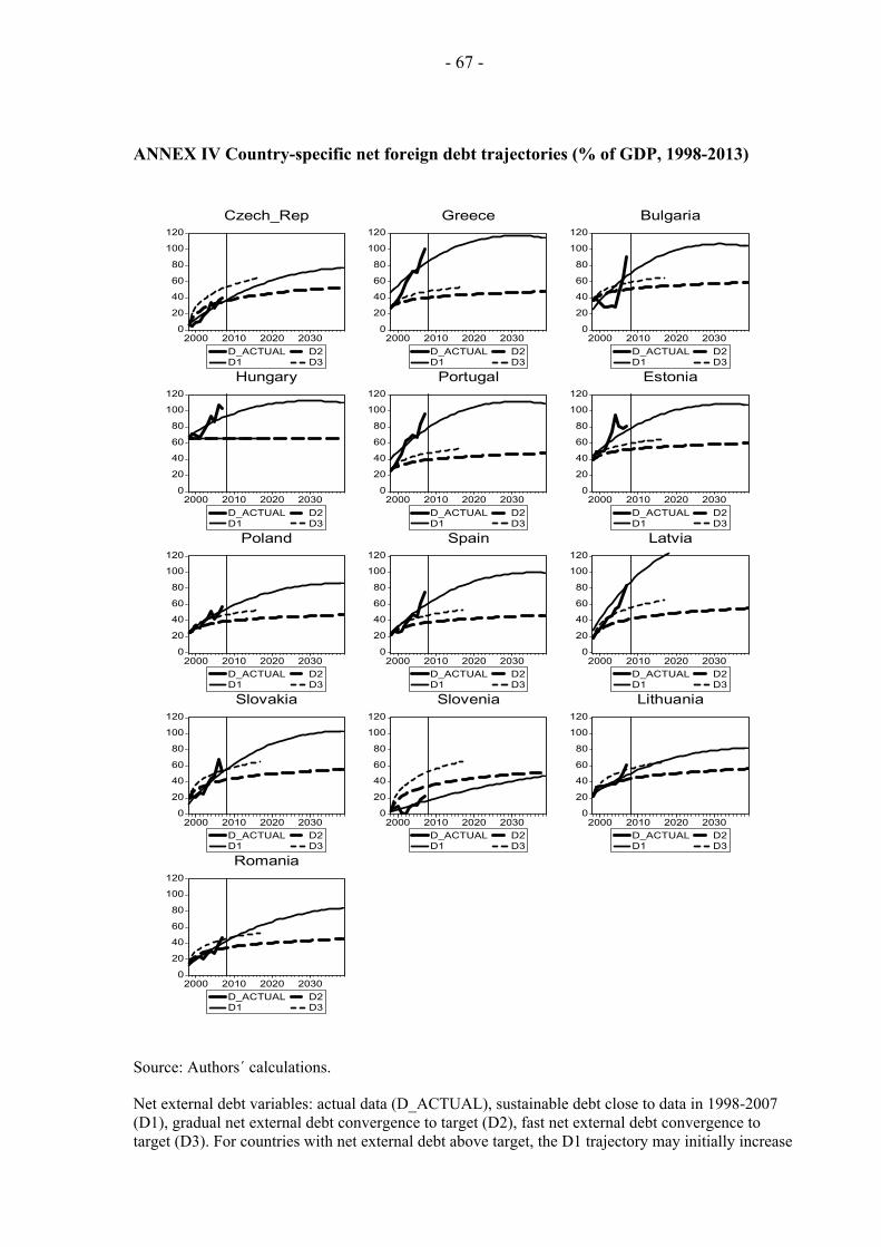
- 67 -

ANNEX IV Country-specific net foreign debt trajectories (% of GDP, 1998-2013)

0

20

40

60

80

100

120

2000 2010 2020 2030D_ACTUALD1

D2D3

Czech_Rep

0

20

40

60

80

100

120

2000 2010 2020 2030D_ACTUALD1

D2D3

Greece

0

20

40

60

80

100

120

2000 2010 2020 2030D_ACTUALD1

D2D3

Bulgaria

0

20

40

60

80

100

120

2000 2010 2020 2030D_ACTUALD1

D2D3

Hungary

0

20

40

60

80

100

120

2000 2010 2020 2030D_ACTUALD1

D2D3

Portugal

0

20

40

60

80

100

120

2000 2010 2020 2030D_ACTUALD1

D2D3

Estonia

0

20

40

60

80

100

120

2000 2010 2020 2030D_ACTUALD1

D2D3

Poland

0

20

40

60

80

100

120

2000 2010 2020 2030D_ACTUALD1

D2D3

Spain

0

20

40

60

80

100

120

2000 2010 2020 2030D_ACTUALD1

D2D3

Latvia

0

20

40

60

80

100

120

2000 2010 2020 2030D_ACTUALD1

D2D3

Slovakia

0

20

40

60

80

100

120

2000 2010 2020 2030D_ACTUALD1

D2D3

Slovenia

0

20

40

60

80

100

120

2000 2010 2020 2030D_ACTUALD1

D2D3

Lithuania

0

20

40

60

80

100

120

2000 2010 2020 2030D_ACTUALD1

D2D3

Romania

Source: Authors´ calculations.

Net external debt variables: actual data (D_ACTUAL), sustainable debt close to data in 1998-2007 (D1), gradual net external debt convergence to target (D2), fast net external debt convergence to target (D3). For countries with net external debt above target, the D1 trajectory may initially increase

- 68 -

above the target, but converges to it in longer horizon, not pictured here.

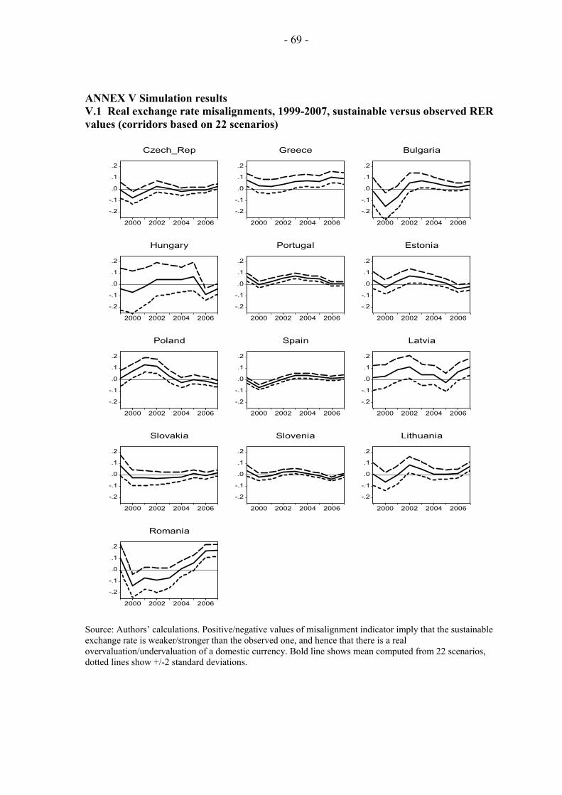
- 69 -

ANNEX V Simulation results V.1 Real exchange rate misalignments, 1999-2007, sustainable versus observed RER values (corridors based on 22 scenarios)

-.2

-.1

.0

.1

.2

2000 2002 2004 2006

Czech_Rep

-.2

-.1

.0

.1

.2

2000 2002 2004 2006

Greece

-.2

-.1

.0

.1

.2

2000 2002 2004 2006

Bulgaria

-.2

-.1

.0

.1

.2

2000 2002 2004 2006

Hungary

-.2

-.1

.0

.1

.2

2000 2002 2004 2006

Portugal

-.2

-.1

.0

.1

.2

2000 2002 2004 2006

Estonia

-.2

-.1

.0

.1

.2

2000 2002 2004 2006

Poland

-.2

-.1

.0

.1

.2

2000 2002 2004 2006

Spain

-.2

-.1

.0

.1

.2

2000 2002 2004 2006

Latvia

-.2

-.1

.0

.1

.2

2000 2002 2004 2006

Slovakia

-.2

-.1

.0

.1

.2

2000 2002 2004 2006

Slovenia

-.2

-.1

.0

.1

.2

2000 2002 2004 2006

Lithuania

-.2

-.1

.0

.1

.2

2000 2002 2004 2006

Romania

Source: Authors’ calculations. Positive/negative values of misalignment indicator imply that the sustainable exchange rate is weaker/stronger than the observed one, and hence that there is a real overvaluation/undervaluation of a domestic currency. Bold line shows mean computed from 22 scenarios, dotted lines show +/-2 standard deviations.

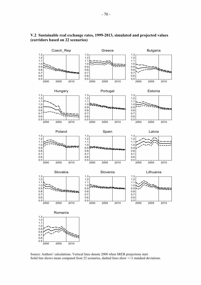
- 70 -

V.2 Sustainable real exchange rates, 1999-2013, simulated and projected values (corridors based on 22 scenarios)

0.50.60.70.80.91.01.11.21.3

2000 2005 2010

Czech_Rep

0.50.60.70.80.91.01.11.21.3

2000 2005 2010

Greece

0.50.60.70.80.91.01.11.21.3

2000 2005 2010

Bulgaria

0.50.60.70.80.91.01.11.21.3

2000 2005 2010

Hungary

0.50.60.70.80.91.01.11.21.3

2000 2005 2010

Portugal

0.50.60.70.80.91.01.11.21.3

2000 2005 2010

Estonia

0.50.60.70.80.91.01.11.21.3

2000 2005 2010

Poland

0.50.60.70.80.91.01.11.21.3

2000 2005 2010

Spain

0.50.60.70.80.91.01.11.21.3

2000 2005 2010

Latvia

0.50.60.70.80.91.01.11.21.3

2000 2005 2010

Slovakia

0.50.60.70.80.91.01.11.21.3

2000 2005 2010

Slovenia

0.50.60.70.80.91.01.11.21.3

2000 2005 2010

Lithuania

0.50.60.70.80.91.01.11.21.3

2000 2005 2010

Romania

Source: Authors’ calculations. Vertical lines denote 2008 when SRER projections start. Solid line shows mean computed from 22 scenarios, dashed lines show +/-2 standard deviations.

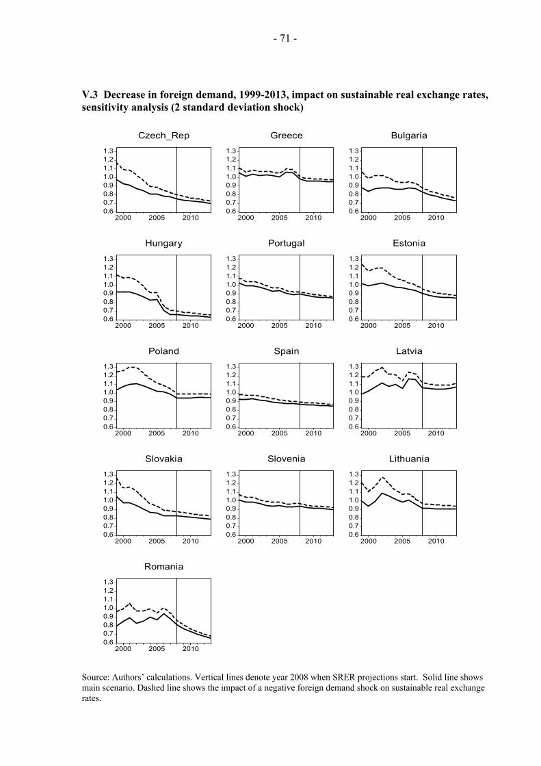
- 71 -

V.3 Decrease in foreign demand, 1999-2013, impact on sustainable real exchange rates, sensitivity analysis (2 standard deviation shock)

0.60.70.80.91.01.11.21.3

2000 2005 2010

Czech_Rep

0.60.70.80.91.01.11.21.3

2000 2005 2010

Greece

0.60.70.80.91.01.11.21.3

2000 2005 2010

Bulgaria

0.60.70.80.91.01.11.21.3

2000 2005 2010

Hungary

0.60.70.80.91.01.11.21.3

2000 2005 2010

Portugal

0.60.70.80.91.01.11.21.3

2000 2005 2010

Estonia

0.60.70.80.91.01.11.21.3

2000 2005 2010

Poland

0.60.70.80.91.01.11.21.3

2000 2005 2010

Spain

0.60.70.80.91.01.11.21.3

2000 2005 2010

Latvia

0.60.70.80.91.01.11.21.3

2000 2005 2010

Slovakia

0.60.70.80.91.01.11.21.3

2000 2005 2010

Slovenia

0.60.70.80.91.01.11.21.3

2000 2005 2010

Lithuania

0.60.70.80.91.01.11.21.3

2000 2005 2010

Romania

Source: Authors’ calculations. Vertical lines denote year 2008 when SRER projections start. Solid line shows main scenario. Dashed line shows the impact of a negative foreign demand shock on sustainable real exchange rates.