peak load energy management by direct load control contracts · peak load energy management by...
TRANSCRIPT

Submitted to Operations Researchmanuscript (Please, provide the manuscript number!)
Peak Load Energy Management by Direct LoadControl Contracts
Ali FattahiAnderson School of Management, University of California, Los Angeles, Los Angeles, California 90095,
Sriram DasuMarshall School of Business, University of Southern California, Los Angeles, Los Angeles, California 90089,
Reza AhmadiAnderson School of Management, University of California, Los Angeles, Los Angeles, California 90095,
Energy firms use demand-response programs such as direct load control contracts (DLCCs) to curtail
electricity consumption during peak load periods. We study contracts that allow utilities to directly reduce
customers’ consumption via remote control devices. Regulators limit the number of times (calls) in a year
a customer’s power consumption can be reduced, the duration of each call, and the total number of hours
of power reduction over the life of the contract. For technical reasons, utilities partition customers that
enroll in DLCCs into groups. To optimally implement DLCCs, utilities have to solve a stochastic dynamic
optimization problem each day that determines how many groups to call and the timing and duration of
each call. This is a provably difficult optimization problem. A practically appealing version of DLCCs is one
in which all calls are restricted to the same duration. Under this restriction, we show that the problem has a
special structure that enables us to find optimal solutions. We develop a near-optimum heuristic procedure
for the general stochastic problem. There are two simplifications in our approximation scheme. First, we
aggregate the groups into a single group, which allows us to reduce the state space. Second, we ignore the
detailed structure of the uncertainty. We refer to the error induced by these two schemes as aggregation
and information error, respectively. The asymptotic relative error, which includes the information error
(O(1/√n)) and the aggregation error (O(1/n)), is shown to be zero. The effectiveness of our proposed
solution procedures is also verified numerically. Finally, applying our heuristic to an industrial instance from
the Southern California region results in approximately 8% saving in the energy generation cost.
Subject classifications: Electric Industries. Dynamic programming. Stochastic Programming.
1

Fattahi, Dasu and Ahmadi: Peak Load Energy Management2 Article submitted to Operations Research; manuscript no. (Please, provide the manuscript number!)
1. Introduction
For energy firms, matching supply and demand is challenging due to variability in demand, large
fluctuations in cost among alternative power generation methods, and the inability to store power.
Power consumption is often weather dependent and varies by hour of day. High demand can cause
grid failure, which is estimated to cost tens of billions of dollars per year.1 Inability to meet demand,
besides being unacceptable, results in significant direct and indirect financial penalties for the
utilities (Taylor and Taylor 2015).
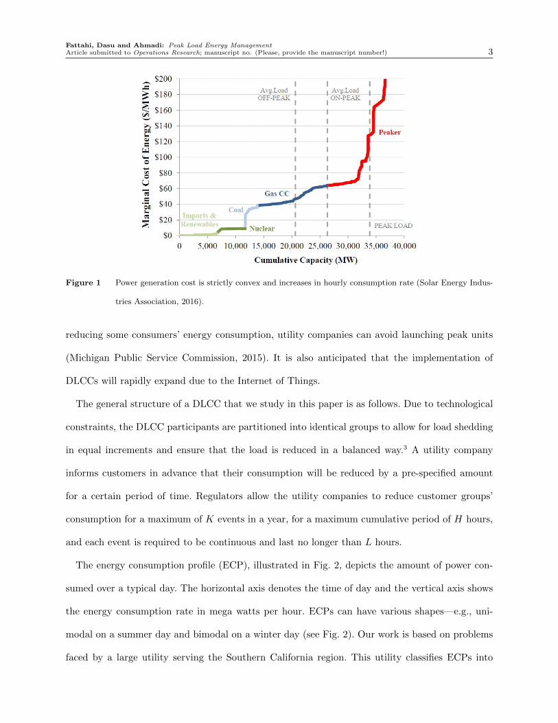
Supply costs are highly non-linear (see Fig. 1, and Meulemeester (2014), Posner (2015), Next-
Kraftwerke-Belgium (2016)). When demand rises above amounts that can be supplied by primary
power generators such as renewable (Alizamir et. al 2016), nuclear, coal, and gas, secondary sources
such as diesel and gasoline-powered generators are used. Peak period refers to the time interval
when demand exceeds primary generators’ capacity and peak units must be activated. As indicated
in Fig. 1, peak units are significantly more expensive. The U.S. Government Accountability Office
finds that the cost of generating electricity during hot summer days is about 10 times higher than
at night. The top 100-highest priced hours in one year account for nearly 20% of the total energy
cost.2 Therefore, dynamic demand management during peak periods is central to matching supply
and demand in this industry.
Utilities have introduced a number of programs that reduce or shift the peak load through a
pricing mechanism (Peura and Bunn 2015, Baldick et. al 2006, Kamat and Oren 2002) or by direct
load control contracts (DLCCs) (Oren and Smith 1992). In this paper, we concentrate on DLCCs,
which are very popular in developed countries and, according to the Federal Energy Regulatory
Commission, in the U.S., “as of 2012, more than 200 utilities across the country offered some type
of direct load control program for residential customers” (Michigan Public Service Commission,
2015). DLCCs permit utility companies to directly reduce a customer’s energy usage using a remote
control device that is installed on site. In residential areas, DLCCs usually target central air
conditioning systems, controlled electric appliances, electric water heaters, and pool pumps. By
Fattahi, Dasu and Ahmadi: Peak Load Energy ManagementArticle submitted to Operations Research; manuscript no. (Please, provide the manuscript number!) 3
Figure 1 Power generation cost is strictly convex and increases in hourly consumption rate (Solar Energy Indus-
tries Association, 2016).
reducing some consumers’ energy consumption, utility companies can avoid launching peak units
(Michigan Public Service Commission, 2015). It is also anticipated that the implementation of
DLCCs will rapidly expand due to the Internet of Things.
The general structure of a DLCC that we study in this paper is as follows. Due to technological
constraints, the DLCC participants are partitioned into identical groups to allow for load shedding
in equal increments and ensure that the load is reduced in a balanced way.3 A utility company
informs customers in advance that their consumption will be reduced by a pre-specified amount
for a certain period of time. Regulators allow the utility companies to reduce customer groups’
consumption for a maximum of K events in a year, for a maximum cumulative period of H hours,
and each event is required to be continuous and last no longer than L hours.
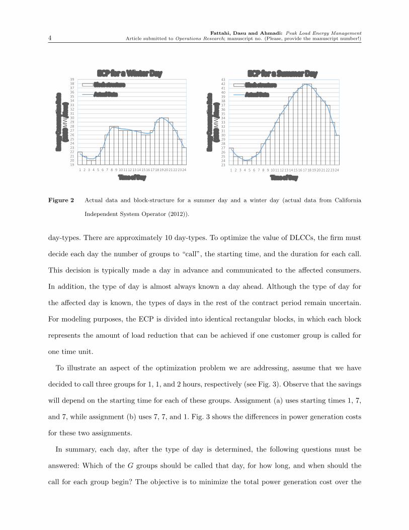
The energy consumption profile (ECP), illustrated in Fig. 2, depicts the amount of power con-
sumed over a typical day. The horizontal axis denotes the time of day and the vertical axis shows
the energy consumption rate in mega watts per hour. ECPs can have various shapes—e.g., uni-
modal on a summer day and bimodal on a winter day (see Fig. 2). Our work is based on problems
faced by a large utility serving the Southern California region. This utility classifies ECPs into
Fattahi, Dasu and Ahmadi: Peak Load Energy Management4 Article submitted to Operations Research; manuscript no. (Please, provide the manuscript number!)
192021222324252627282930313233343536373839
1 2 3 4 5 6 7 8 9 10 11 12 13 14 15 16 17 18 19 20 21 22 23 24
Ener
gy C
onsu
mpt
ion
Rate
(1
000 MW
/Hou
r)
Time of Day
ECP for a Winter DayBlock-structure
Actual Data
232425262728293031323334353637383940414243
1 2 3 4 5 6 7 8 9 10 11 12 13 14 15 16 17 18 19 20 21 22 23 24
Ener
gy C
onsu
mpt
ion
Rate
(1
000 MW
/Hou
r)
Time of Day
ECP for a Summer DayBlock-structure
Actual Data
Figure 2 Actual data and block-structure for a summer day and a winter day (actual data from California
Independent System Operator (2012)).
day-types. There are approximately 10 day-types. To optimize the value of DLCCs, the firm must
decide each day the number of groups to “call”, the starting time, and the duration for each call.
This decision is typically made a day in advance and communicated to the affected consumers.
In addition, the type of day is almost always known a day ahead. Although the type of day for
the affected day is known, the types of days in the rest of the contract period remain uncertain.
For modeling purposes, the ECP is divided into identical rectangular blocks, in which each block
represents the amount of load reduction that can be achieved if one customer group is called for
one time unit.
To illustrate an aspect of the optimization problem we are addressing, assume that we have
decided to call three groups for 1, 1, and 2 hours, respectively (see Fig. 3). Observe that the savings
will depend on the starting time for each of these groups. Assignment (a) uses starting times 1, 7,
and 7, while assignment (b) uses 7, 7, and 1. Fig. 3 shows the differences in power generation costs
for these two assignments.
In summary, each day, after the type of day is determined, the following questions must be
answered: Which of the G groups should be called that day, for how long, and when should the
call for each group begin? The objective is to minimize the total power generation cost over the

Fattahi, Dasu and Ahmadi: Peak Load Energy ManagementArticle submitted to Operations Research; manuscript no. (Please, provide the manuscript number!) 5
1 42 23 14 15 26 17 58 19 1
10 1 0
1
2
3
4
5
1 2 3 4 5 6 7 8 9 10
Ener
gy C
onsu
mpt
ion
Rate
Time of Day
Assignment (b)
0
1
2
3
4
5
1 2 3 4 5 6 7 8 9 10
Ener
gy C
onsu
mpt
ion
Rate
Time of Day
Assignment (a)
Figure 3 An example: Assigning 3 calls with lengthes 1, 1, and 2 to customer groups.
contract horizon, which is equivalent to maximizing the total saving. The constraints are (i) each
group of customers is called no more than K times in a year, (ii) the duration of each call is less
than L hours, (iii) the power reduction must occur over a continuous interval, and (iv) the total
number of hours of load reduction for a group in a year cannot exceed H hours.
We refer to our problem as the general stochastic problem (GSP), in which the uncertainty in the
type of day is modeled via multi-nomial distributions. The GSP can be viewed as a general version
of the revenue management problem (Adelman 2007, Zhang and Adelman 2009, Cooper 2002).
Specifically, with one customer group, the GSP reduces to the well-known revenue management
problem (Jasin and Kumar 2012). The GSP with two groups is weakly NP-complete and with
G groups is strongly NP-complete. The GSP is a finite-horizon stochastic dynamic program with
a 2G-dimensional state space. The state space is the number of available calls and hours for
each group. We present a heuristic approach (HGSP) that is based on two approximations: (i)
ignoring uncertainty which creates information error, and (ii) ignoring group identities which
creates aggregation error. Our analysis of the information error adapts the approach of Jasin
and Kumar (2012). We show that the worst-case relative performance of the information and
aggregation errors are O(1/√n) and O(1/n), respectively, where n denotes the problem size.
The power company that we are working with is interested in a policy in which all calls are of
the same duration. The corresponding problem is referred to as the fixed-length stochastic problem
(FSP). We present a polynomial time algorithm to find an optimal solution to the FSP.
The remainder of the paper is organized as follows. Section 2 presents the mathematical formu-
lation of our problem and establishes its NP-completeness. In Section 3, we present a polynomial

Fattahi, Dasu and Ahmadi: Peak Load Energy Management6 Article submitted to Operations Research; manuscript no. (Please, provide the manuscript number!)
time algorithm to solve the FSP. Sections 4 and 5 present our heuristic approach to solve the GSP,
study its theoretical properties, and establish its worst-case error bounds. In Section 6, we test the
effectiveness of the HGSP and solve an industrial instance of the problem. Finally, we conclude the
paper and offer some directions for future work.
2. Problem Formulation
The GSP is a finite-horizon stochastic dynamic program in which stages correspond to the days
in the planning horizon d= 1, . . . ,D. For a complete list of notations, see Appendix F. The index
d refers to the beginning of a day and, hence, d = 1 is the beginning of the planning horizon.
Uncertainty is induced by day-type ω ∈Ω. The state variables are the remaining number of calls
and hours for each group. As previously stated, a decision is made each day to determine which
groups to call, the duration of the calls, and the starting time for each call.
There are G identical groups that are indexed as g = 1, . . . ,G. Group g can be called on day d
for a duration of ldg hours, satisfying 0≤ ldg ≤L. Let mdg be a binary variable that shows if group
g is called on day d. If ldg > 0, then mdg = 1, and otherwise mdg = 0.
We define vectors Ld = (ld1, . . . , ldG) and Md = (md1, . . . ,mdG), for all d, which respectively
show the duration of calls and whether each group is called on day d. We define vectors Hd =
(hd1, . . . , hdG) and Kd = (kd1, . . . , kdG), for all d, which respectively show the number of calls avail-
able and the duration of time available from each group on day d. At the beginning of the planning
horizon d= 1, we have H1 = (H, . . . ,H) and K1 = (K, . . . ,K), which represent identical contracts
of groups.
Let the augmented vector (Ld,Md) denote a decision on day d. Let Θd denote the set of
feasible decisions on day d. We define Θd := (Ld,Md)| mdg ≤ kdg, ldg ≤ minhdg,L, mdg =
I(ldg), for all g, for all d. Here, I(.) is the indicator function: I(ldg) = 1 if ldg > 0, and otherwise
I(ldg) = 0. The finite-horizon stochastic dynamic program for the GSP is as follows:
Vd(Hd,Kd) = min(Ld,Md)∈Θd
ψ(Ld, ωd) +
E [Vd+1(Hd−Ld,Kd−Md)], ∀d= 1, . . . ,D− 1,
VD(HD,KD) = min(LD,MD)∈ΘD
ψ(LD, ωD), (1)

Fattahi, Dasu and Ahmadi: Peak Load Energy ManagementArticle submitted to Operations Research; manuscript no. (Please, provide the manuscript number!) 7
where, Vd(Hd,Kd) is the optimal cost for days d, d + 1, . . . ,D given Hd available time and Kd
available number of calls. Finally, ψ(Ld, ωd) denotes the minimum cost that one could achieve in
day d, which is found by solving a mixed integer linear programming (MILP) problem (see Section
2.1).
2.1. Single day problem
We present an MILP formulation to obtain ψ(Ld, ωd). This MILP is referred to as the single day
problem (SDP).Each day consists of T time periods—e.g., 24 hours. Let t denote the index for
time periods in a day. We assume that the ECP height is constant during time period t on day
d and is given by function rt : Ω−→ Z+, and hence rt(ωd) is the ECP height in period t and day
d. Moreover, the energy cost in period t and day d depends solely on rt(ωd), which is given by
the function f : Z+ −→R. For each z ∈ Z, z ≥ 1, we define ∂f(z) := f(z)− f(z− 1) and ∂2f(z) :=
∂f(z)− ∂f(z − 1). We assume that the cost function satisfies: (i) f(0) = ∂f(0) = ∂2f(0) = 0, (ii)
∂f(z) > 0, for all z ∈ Z, z ≥ 1, and (iii) ∂2f(z) > 0, for all z ∈ Z, z ≥ 1. Properties (ii) and (iii)
respectively mean that f(z) is strictly increasing in z and that the marginal increase in z is also
strictly increasing in z (as indicated in Fig.1). Finally, note that f does not have index d and/or t
since the energy cost depends solely on the ECP height.
Let binary variables ugt and wgt, for all g and t, be defined as follows: ugt = 1 shows that group g
is on call in period t of day d, and wgt = 1 indicates that group g starts in t. The SDP is formulated
as follows:
ψ(Ld, ωd) = minT∑
t=1
f
[rt(ωd)−
G∑
g=1
ugt
]+ (2)
s.t.T∑
t=1
ugt = ldg, ∀g, (3)
wgt ≥ ugt−ug(t−1), ∀g, t≥ 2, (4)
wg1 ≥ ug1, ∀g, (5)
T∑
t=1
wgt ≤ 1, ∀g, (6)
ugt,wgt ∈ 0,1, ∀g, t, (7)

Fattahi, Dasu and Ahmadi: Peak Load Energy Management8 Article submitted to Operations Research; manuscript no. (Please, provide the manuscript number!)
where, [z]+ := maxz,0. In the objective function (Eq. 2),∑G
g=1 ugt is the number of groups on call
in period t. The ECP height in period t decreases by∑G
g=1 ugt and hence becomes rt(ωd)−∑G
g=1 ugt
if this value is positive, and 0 otherwise. Eq. (3) ensures that group g is called for ldg time units and
Eqs. (4)–(6) guarantee that the reduction occurs over a continuous interval. Eqs. (4)–(5) initialize
the starting time of the calls. Eq. (6) confirms that each group can be called once on day d at most.
We next show that the deterministic version of the GSP, which we refer to as the general
deterministic problem (GDP), is very difficult. The following proposition establishes that special
case of the GDP with two groups is weakly NP-complete and the general case of the GDP is strongly
NP-complete.
Proposition 1. (a) the GDP with G = 2 is weakly NP-complete, and (b) the GDP is strongly
NP-complete.
The proof is standard and follows from a reduction from the partition problem for part (a) and
a reduction from the 3-partition problem in part (b) (see Appendix A). We note that the GDP is
an easier, special case of the GSP because it considers only one realization of day-types; hence, the
GSP is significantly more difficult.
3. Fixed-Length Policy
Due to the ease of implementation, a policy that is used frequently is the fixed-length policy (FLP).
According to this policy, the duration of calls are equal and fixed to L′ hours, where 0≤ L′ ≤ L.
Under the FLP, the energy companies always contract with their customers for H =KL′ hours.
In fact, the constraint on the total hours of energy-consumption reduction is no longer necessary.
We refer to this problem as the fixed-length stochastic problem (FSP), and it includes only the
constraint on the total number of calls per group.
We aggregate the state variables, solve the low-dimensional problem, and disaggregate the solu-
tion. This approach is proven to find an optimal solution for the FSP. The aggregate version of the
FSP is refered to as the aggregate fixed-length stochastic problem (AFSP). Let Kd denote the total
number of calls that we want to assign to groups on day d, and Kd denote the remaining number

Fattahi, Dasu and Ahmadi: Peak Load Energy ManagementArticle submitted to Operations Research; manuscript no. (Please, provide the manuscript number!) 9
of calls at the beginning of day d. Obviously, K1 =GK. On each day d, our decision must satisfy
Kd ≤Kd because we have at most Kd calls to use for the rest of the planning horizon d, d+1, . . . ,D.
Moreover, Kd ≤G, for each day d, because G groups exist and each group can be called at most once
a day. We define the set of feasible decisions for the AFSP as Θafd := Kd ∈Z+|Kd ≤minKd,G,
for all d. Let ψaf(Kd, ωd) be the optimal cost of using Kd on day d. The dynamic programming
(DP) formulation of AFSP is as follows:
Vafd (Kd) = min
Kd∈Θafd
ψaf(Kd, ωd) + E[Vafd+1(Kd−Kd)
], ∀d= 1, · · · ,D− 1,
VafD (KD) = min
KD∈ΘafD
ψaf(KD, ωD), (8)
where, ψaf(Kd, ωd) is the optimal cost of using Kd calls on day d knowing that the day-type is ωd.
We next formulate a mathematical model to determine ψaf(Kd, ωd). This problem is referred to as
the aggregate fixed-length single day problem (AFSDP). Let integer variables st and Rt, for each t,
indicate the number of groups that start reducing their energy consumption at period t, and the
ECP height at period t after customers reduce their energy consumption, respectively. The AFSDP
is formulated as follows:
ψaf(Kd, ωd) = minT∑
t=1
f(Rt), (9)
s.t. Rt ≥ rt(ωd)−minT−L′+1,t∑
t′=max1,t−L′+1st′ , ∀t (10)
T−L′+1∑
t=1
st =Kd (11)
st,Rt ∈Z+, ∀t. (12)
The summation in constraint (10) represents the number of groups that are on call at time t.
Constraint (11) ensures that the total number of groups reducing their consumption on day d is
equal to Kd.
Algorithm 1 presents our approach for solving the FSP. We first solve the AFSDP for all 0≤Kd ≤
GK and ωd ∈Ω and we then solve the AFSP. For each day d, we find a set of calls that is denoted
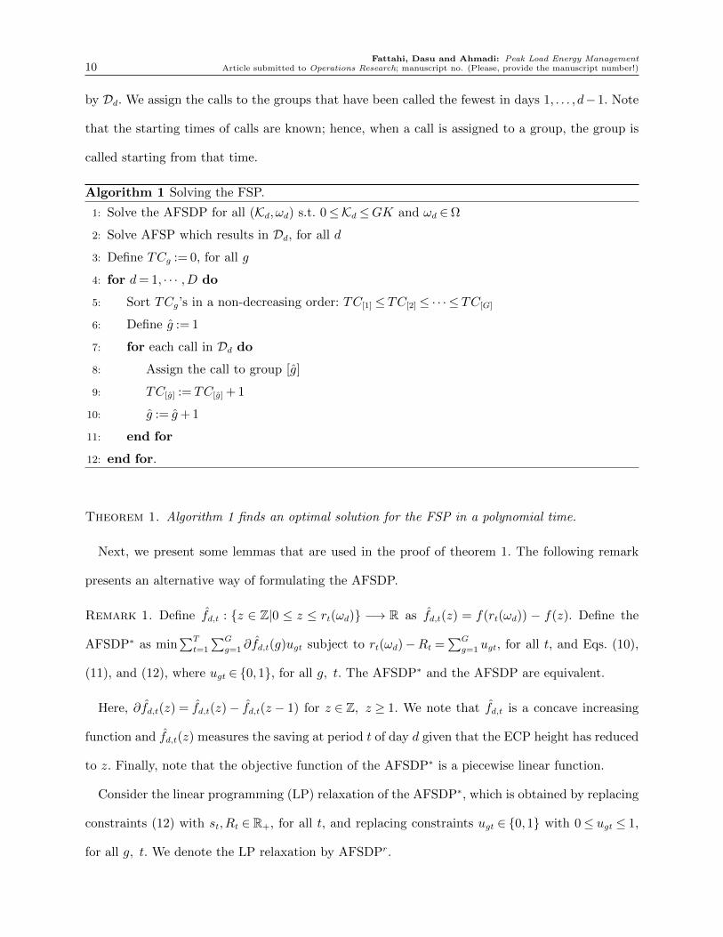
Fattahi, Dasu and Ahmadi: Peak Load Energy Management10 Article submitted to Operations Research; manuscript no. (Please, provide the manuscript number!)
by Dd. We assign the calls to the groups that have been called the fewest in days 1, . . . , d−1. Note
that the starting times of calls are known; hence, when a call is assigned to a group, the group is
called starting from that time.
Algorithm 1 Solving the FSP.
1: Solve the AFSDP for all (Kd, ωd) s.t. 0≤Kd ≤GK and ωd ∈Ω
2: Solve AFSP which results in Dd, for all d
3: Define TCg := 0, for all g
4: for d= 1, · · · ,D do
5: Sort TCg’s in a non-decreasing order: TC[1] ≤ TC[2] ≤ · · · ≤ TC[G]
6: Define g := 1
7: for each call in Dd do
8: Assign the call to group [g]
9: TC[g] := TC[g] + 1
10: g := g+ 1
11: end for
12: end for.
Theorem 1. Algorithm 1 finds an optimal solution for the FSP in a polynomial time.
Next, we present some lemmas that are used in the proof of theorem 1. The following remark
presents an alternative way of formulating the AFSDP.
Remark 1. Define fd,t : z ∈ Z|0 ≤ z ≤ rt(ωd) −→ R as fd,t(z) = f(rt(ωd)) − f(z). Define the
AFSDP∗ as min∑T
t=1
∑G
g=1 ∂fd,t(g)ugt subject to rt(ωd)−Rt =∑G
g=1 ugt, for all t, and Eqs. (10),
(11), and (12), where ugt ∈ 0,1, for all g, t. The AFSDP∗ and the AFSDP are equivalent.
Here, ∂fd,t(z) = fd,t(z)− fd,t(z − 1) for z ∈ Z, z ≥ 1. We note that fd,t is a concave increasing
function and fd,t(z) measures the saving at period t of day d given that the ECP height has reduced
to z. Finally, note that the objective function of the AFSDP∗ is a piecewise linear function.
Consider the linear programming (LP) relaxation of the AFSDP∗, which is obtained by replacing
constraints (12) with st,Rt ∈R+, for all t, and replacing constraints ugt ∈ 0,1 with 0≤ ugt ≤ 1,
for all g, t. We denote the LP relaxation by AFSDPr.

Fattahi, Dasu and Ahmadi: Peak Load Energy ManagementArticle submitted to Operations Research; manuscript no. (Please, provide the manuscript number!) 11
Proposition 2. The AFSDPr solves the AFSDP∗.
Lemma 1. In Algorithm 1, at each iteration d of the for-loop, such that d≤D−1, we have |TCg′−
TCg′′ | ≤ 1 for each pair of groups g′, g′′.
See Appendix B for the proofs. Based on Proposition 2, the AFSDP∗ is solved in a polynomial
time. Moreover, according to Lemma 1, Algorithm 1 assigns calls to groups in an almost balanced
fashion, for all d≤D− 1.
Lemma 2. The solution of Algorithm 1 satisfies TCg ≤K, for all g.
Lemma 2 states that the solution that we obtain by applying Algorithm 1 is feasible.
Proof of Theorem 1. The AFSP is a relaxation of the FSP because the AFSP does not consider
group identities. This means that a feasible solution for the FSP is always feasible for the AFSP;
however, a feasible solution for the AFSP may not be feasible for the FSP. Therefore, to prove the
optimality of the solution, it suffices to show that the obtained solution is feasible for the FSP. For
this, we must prove that the use of for -loop for assigning the solution of each day Dd to groups does
not violate the maximum number of calls per group constraint. This is proven in Lemma 2. Thus,
Algorithm 1 finds an optimal solution for the FSP. Note that once the solution of the AFSDP for
all 0≤Kd ≤GK and ωd ∈Ω is given, which is found in a polynomial time (see Proposition 2), the
rest of the algorithm requires a polynomial time. Therefore, the proof of theorem 1 is complete.
4. General Stochastic Problem (GSP)
Solving the GSP is difficult because of the stochasticity and 2G-dimensional state space. We present
an effective heuristic approach, which is denoted by HGSP, to solve the GSP and show that, for a
sufficiently large problem size, the error is negligible. The main steps of the HGSP are as follows: (1)
aggregating state space to obtain the aggregate general stochastic problem (AGSP), (2) fixing the
number of days of each type to their expected value, to obtain the aggregate general deterministic
problem (AGDP), (3) solving the AGDP in a polynomial time using a DP algorithm, and, (4)
disaggregating the AGDP solution.

Fattahi, Dasu and Ahmadi: Peak Load Energy Management12 Article submitted to Operations Research; manuscript no. (Please, provide the manuscript number!)
To analyze the asymptotic behavior of our heuristic approach for sufficiently large D, K, and
H, we define n∈Z, n≥ 1 to represent the problem size. We consider a series of problems with nD
days, nK calls, and nH hours per group for all n ∈ Z, n≥ 1. We aim to show that our heuristic
approach finds an asymptotically optimal solution to the GSP. Let v(n)GSP denote the optimal saving
for the GSP, v(n)HGSP denote the HGSP saving, v
(n)AGDP denote the optimal saving for the AGDP, and
v(n)AGSP denote the optimal saving for the AGSP, where the problem size is n.
Theorem 2. E[v(n)GSP]− v(n)HGSP =O(
√n) for all n∈Z, n≥ 1.
Thus, as n −→∞, the relative error approaches to zero. The proof of theorem 2 follows from
noting that the difference between E[v(n)GSP] and v
(n)HGSP includes two types of error—information
error and aggregation error—and finding upper bounds on these errors. Information error refers
to the error that is created from replacing random variables with their expected values.
Theorem 3 (Information Error). v(n)AGDP−E[v
(n)AGSP] =O(
√n) for all n∈Z, n≥ 1.
The proof of theorem 3 is deferred to Section 4.1. The second type of error in HGSP is called
aggregation error, which is created from aggregating the state space in step (2).
Theorem 4 (Aggregation Error). There exists a non-negative constant ρ, independent of n,
such that v(n)AGDP− v(n)HGSP ≤ ρ and E[v
(n)AGSP]−E[v
(n)GSP]≤ ρ, for all n∈Z, n≥ 1.
The proof of theorem 4 is deferred to Section 5.3. Theorem 4 states that there exists a constant
upper bound on the aggregation error that does not increase in n; hence, the relative aggregation
error is O( 1n
). Finally, the proof of theorem 2 follows from theorems 3 and 4.
4.1. Information error
Information error is referred to the difference between the optimal value of the AGDP and the
expected optimal value of the AGSP. Here, the AGDP considers pωD days of type ω for each ω ∈Ω,
where pω denotes the proportion of days of type ω (the probability of day-type ω). We assume pωD
is an integer for all ω, which is a reasonable assumption because pωD is the expected number of
days of type ω. We show that the absolute information error is O(√n).

Fattahi, Dasu and Ahmadi: Peak Load Energy ManagementArticle submitted to Operations Research; manuscript no. (Please, provide the manuscript number!) 13
In the AGSP, at the beginning of each day, the day-type is revealed. We want to determine the
total number of calls and hours that should be used for that day. The AGSP is an special case of
finite horizon revenue management problems (see, for example, Jasin and Kumar (2012), Cooper
(2002)). The day-type resembles “customer type,” and the total number of calls and hours that
we use in a day resembles the “offers.” Let “offers” be indexed by j = 1, . . . , J . Different offers
are distinguished by the number of calls, number of hours, and their day-types. In total, we have
J = |Ω|G2L+1 different “offers” from which we can choose one to “make” in a day. We also include
a no-offer scenario that explains the “+1” in the total number of available offers. Each offer can
be used in only one day-type; hence, we use the notation ω(j) to denote the day-type in which
offer j can be used. Once offer j is made, a saving of θj is realized with probability 1, where θj is
found by solving the aggregate single day problem (see Section 5.1). We use index γ = 1, . . . ,Γ to
denote resources. In the AGSP, we have Γ = 2, which are the total number of calls and hours in the
aggregate sense. Let aγj ≥ 0 show the amount of resource γ used when offer j is made, and cγ denote
the total available resource γ at the beginning of the planning horizon. Let aγ := (aγ1, . . . , aγJ) and
aγ,max := maxjaγj for all γ.
To analyze the asymptotic behavior of the error, we use superscript (n) to denote scaling by
factor n, where n∈Z, n≥ 1; hence, the AGSP(n) and the AGDP(n) respectively denote the AGSP
and the AGDP with c(n)γ = ncγ , for all γ, and D(n) = nD. The superscript (n) is dropped whenever
n= 1.
Our analysis of the information error adapts the approach of Jasin and Kumar (2012). They con-
sider a network revenue management problem with uncertain customer choice, where the customer
arrival is modeled via Poisson processes. They show that the expected revenue loss is bounded by
a constant, independent of the problem size, when the problem is re-solved according to a pre-
determined schedule. Whereas in our problem, the day-type, which is analogous to the customer
type is modeled via multi-nomial distributions. We establish that the absolute information error
is O(√n), when the problem is solved once in the beginning of the planning horizon.
Fattahi, Dasu and Ahmadi: Peak Load Energy Management14 Article submitted to Operations Research; manuscript no. (Please, provide the manuscript number!)
The LP relaxation of the AGDP(n) is denoted by the RAGDP(n), which is formulated as follows.
Here, xj denotes the number of times that offer j is made in the planning horizon (xj can be
fractional):
max∑
j
θjxj (13)
s.t.∑
j
aγjxj ≤ ncγ , ∀γ, (14)
∑
j:ω(j)=ω
xj ≤ npωD, ∀ω, (15)
xj ∈R+, ∀j. (16)
Let the optimal solution of the RAGDP(n) be denoted by x∗(n) = (x∗1(n), . . . , x∗J
(n)). Moreover, let
v(n)RAGDP denote the optimal value of the RAGDP(n). Note that x∗(n) = nx∗ for all n≥ 1. Moreover,
v(n)RAGDP provides an upper bound on the optimal value of the AGDP(n).
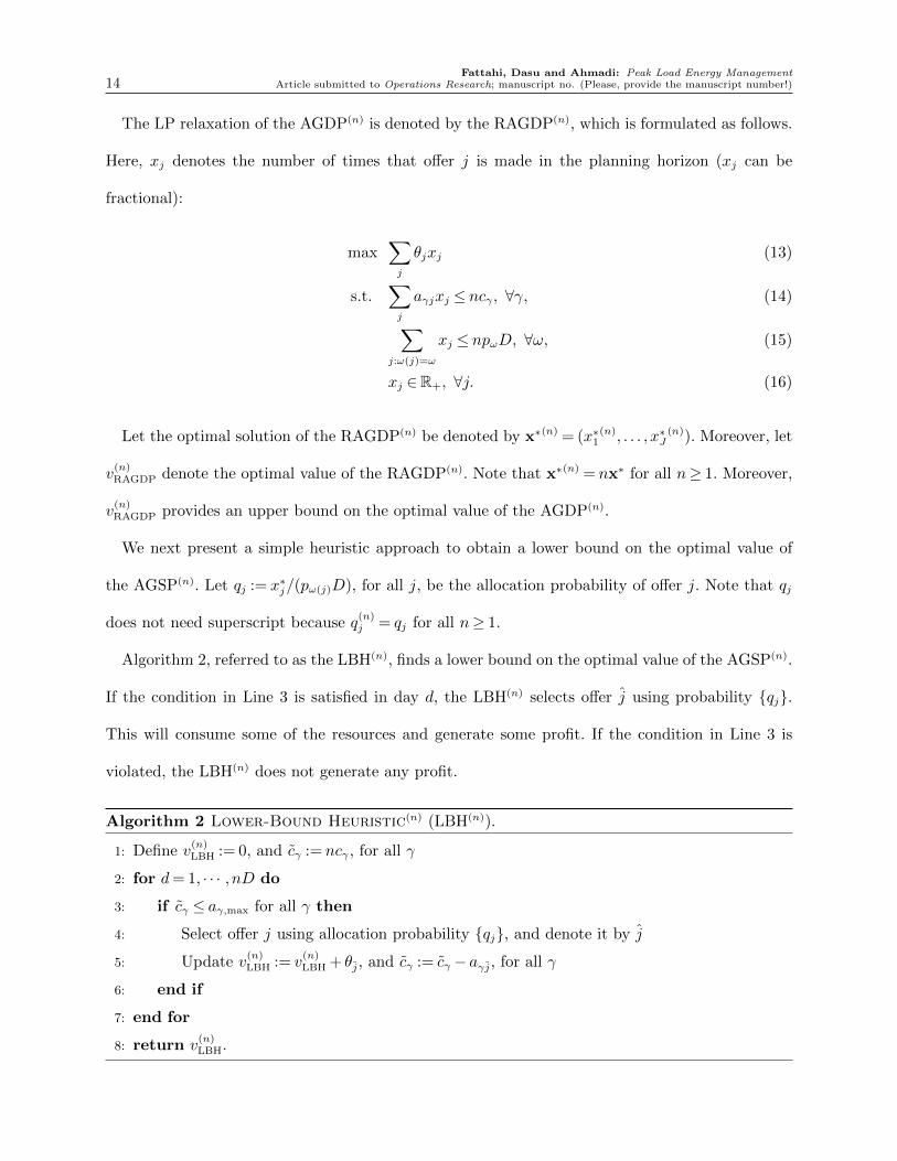
We next present a simple heuristic approach to obtain a lower bound on the optimal value of
the AGSP(n). Let qj := x∗j/(pω(j)D), for all j, be the allocation probability of offer j. Note that qj
does not need superscript because q(n)j = qj for all n≥ 1.
Algorithm 2, referred to as the LBH(n), finds a lower bound on the optimal value of the AGSP(n).
If the condition in Line 3 is satisfied in day d, the LBH(n) selects offer j using probability qj.
This will consume some of the resources and generate some profit. If the condition in Line 3 is
violated, the LBH(n) does not generate any profit.
Algorithm 2 Lower-Bound Heuristic(n) (LBH(n)).
1: Define v(n)LBH := 0, and cγ := ncγ , for all γ
2: for d= 1, · · · , nD do
3: if cγ ≤ aγ,max for all γ then
4: Select offer j using allocation probability qj, and denote it by j
5: Update v(n)LBH := v
(n)LBH + θj, and cγ := cγ − aγj, for all γ
6: end if
7: end for
8: return v(n)LBH.

Fattahi, Dasu and Ahmadi: Peak Load Energy ManagementArticle submitted to Operations Research; manuscript no. (Please, provide the manuscript number!) 15
We introduce an upper-bound heuristic, given in Algorithm 3, in a similar fashion, ignoring
resource constraints. In each day, the UBH(n) selects an offer j with probability qj and realizes
the corresponding profit θj.
Algorithm 3 Upper-Bound Heuristic(n) (UBH(n)).
1: Define v(n)UBH := 0
2: for d= 1, · · · , nD do
3: Select offer j using allocation probability qj, and denote it by j
4: Update v(n)UBH := v
(n)UBH + θj
5: end for
6: return v(n)UBH.
Lemma 3. v(n)AGDP−E[v
(n)AGSP]≤E[v
(n)UBH]−E[v
(n)LBH], for all n∈Z, n≥ 1.
The proof follows from E[v(n)UBH] = v
(n)RAGDP ≥ v(n)AGDP ≥ E[v
(n)AGSP] ≥ E[v
(n)LBH], for all n ∈ Z, n ≥ 1,
and is given in Appendix C. In the remainder, we find an upper bound on E[v(n)UBH]−E[v
(n)LBH] that
is also valid as an upper bound for the information error.
For any realization of the day-types, the LBH(n) and UBH(n) produce equal profits on all days as
long as the condition in Line 3, Algorithm 2, is satisfied. Let d∗(n) denote the minimum of nD and
the last day in which this condition is satisfied. The expected value of profit that is then produced
by the LBH(n) and UBH(n) during days 1,2, . . . , d∗(n) is equivalent. In days d∗(n) + 1, . . . , nD, the
UBH(n) produces profit but the LBH(n) does not. Hence, E[v(n)UBH]−E[v
(n)LBH]≤ θmaxE[nD− d∗(n)],
where θmax := maxjθj. We note that E[d∗(n)] =∑nD
d=1P (d∗(n) ≥ d). Therefore, E[nD − d∗(n)] =
∑nD
d=1P (d∗(n) <d), and we have:
E[v(n)UBH]−E[v
(n)LBH]≤ θmax
nD∑
d=1
P (d∗(n) <d), n∈Z, n≥ 1. (17)
Thus, it remains to obtain an upper bound on P (d∗(n) < d), for all n and d. On each day, after
knowing the day-type, the UBH(n) makes an offer based on probability qj and then some of the
resources are utilized. Although the expected value of the resource usage isaγx∗
D, for all γ and d, the

Fattahi, Dasu and Ahmadi: Peak Load Energy Management16 Article submitted to Operations Research; manuscript no. (Please, provide the manuscript number!)
actual utilization of resource γ on day d isaγx∗
D+ ∆(n)
γ (d), where ∆(n)γ (d) is the deviation from the
expected utilization. We note that ∆(n)γ (d) is a discrete random variable that follows a multi-nomial
distribution with 1 trial and event probability pω(j)qj. Let =d denote the accumulated information
up to day d. Then, ∑d
d′=1 ∆(n)γ (d′)nDd=1 and |∑d
d′=1 ∆(n)γ (d′)|nDd=1 are respectively martingale and
submartingale with respect to filtration =d. Note that E[∑d
d′=1 ∆(n)γ (d′)|=d] = 0, for all n and d.
The following lemma provides an upper bound on the second moment of∑d
d′=1 ∆(n)γ (d′) conditional
on the filtration =d.
Lemma 4. E[(∑d
d′=1 ∆(n)γ (d′))2|=d]≤ 1
4a2γ,maxd, for all γ and d.
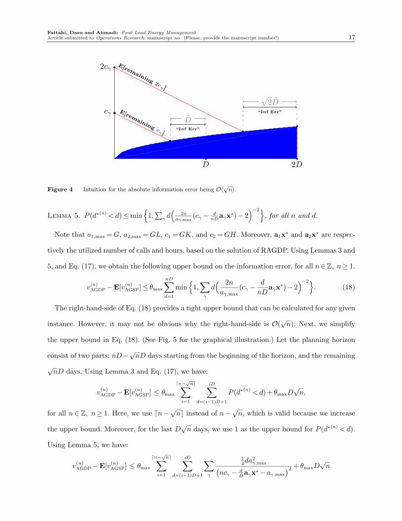
We next provide an intuition for the information error being O(√n) by comparing n = 1 and
n= 2 (see Fig. 4). Consider P (|∑d
d′=1 ∆(n)γ (d′)|> κ) = ϑ, where ϑ is a significantly small positive
number. For this equation to hold for all d, κ must be a linear function of the standard deviation
of |∑d
d′=1 ∆(n)γ (d′)|. Hence, using Lemma 4, κ must be a linear function of
√d. Therefore, in Fig.
4, the shaded area indicates a region where |∑d
d′=1 ∆(n)γ (d′)| would fall with probability 1−ϑ. On
the other hand, consider a resource γ for which the corresponding resource constraint is binding
(a similar argument can be made for the non-binding constraints). Thus, the expected value of
the remaining resource γ decreases linearly in d, from ncγ to 0. We can roughly assume that the
LBH(n) stops offering when the expected value of the remaining resource γ hits the shaded region.
Moreover, the information error is related to the days after this hitting time. The number of days
after the hitting time for n= 1 and n= 2 are D and√
2D, respectively. Therefore, the information
error is O(√n). We next rigorously prove this result.
Given that the LBH(n) makes an offer on day d, the utilization of γ during days 1,2, . . . , d is given
by dD
aγx∗ +
∑d
d′=1 ∆(n)γ (d′). Recall that, for all γ, the total available resource γ at the beginning
of the planning horizon is ncγ . Thus, the condition for LBH(n) to make an offer on day d+ 1 is as
follows:
Condition (†) :d∑
d′=1
∆(n)γ (d′)≤ ncγ −
d
Daγx
∗− aγ,max, for all γ.
In the following lemma, we use condition (†) and Doob’s submartingale inequality to present an
upper bound on P (d∗(n) <d), for all n and d.
Fattahi, Dasu and Ahmadi: Peak Load Energy ManagementArticle submitted to Operations Research; manuscript no. (Please, provide the manuscript number!) 17
2D
2cγ E[remaining 2cγ ]
E[remaining cγ ]
D“Inf Err”
√2D
“Inf Err”
D
cγ
Figure 4 Intuition for the absolute information error being O(√n).
Lemma 5. P (d∗(n) <d)≤min
1,∑
γ d(
2naγ,max
(cγ − dnD
aγx∗)− 2
)−2, for all n and d.
Note that a1,max =G, a2,max =GL, c1 =GK, and c2 =GH. Moreover, a1x∗ and a2x
∗ are respec-
tively the utilized number of calls and hours, based on the solution of RAGDP. Using Lemmas 3 and
5, and Eq. (17), we obtain the following upper bound on the information error, for all n∈Z, n≥ 1.
v(n)AGDP−E[v
(n)AGSP]≤ θmax
nD∑
d=1
min
1,∑
γ
d( 2n
aγ,max
(cγ −d
nDaγx
∗)− 2)−2
. (18)
The right-hand-side of Eq. (18) provides a tight upper bound that can be calculated for any given
instance. However, it may not be obvious why the right-hand-side is O(√n). Next, we simplify
the upper bound in Eq. (18). (See Fig. 5 for the graphical illustration.) Let the planning horizon
consist of two parts: nD−√nD days starting from the beginning of the horizon, and the remaining
√nD days. Using Lemma 3 and Eq. (17), we have:
v(n)AGDP−E[v
(n)AGSP] ≤ θmax
dn−√ne∑
i=1
iD∑
d=(i−1)D+1
P (d∗(n) <d) + θmaxD√n,
for all n ∈ Z, n≥ 1. Here, we use dn−√ne instead of n−√n, which is valid because we increase
the upper bound. Moreover, for the last D√n days, we use 1 as the upper bound for P (d∗(n) <d).
Using Lemma 5, we have:
v(n)AGDP−E[v
(n)AGSP] ≤ θmax
dn−√ne∑
i=1
iD∑
d=(i−1)D+1
∑
γ
14da2γ,max(
ncγ − dD
aγx∗− aγ,max
)2 + θmaxD√n

Fattahi, Dasu and Ahmadi: Peak Load Energy Management18 Article submitted to Operations Research; manuscript no. (Please, provide the manuscript number!)
nD
ncγ
0 D 2D. . . dn−√neD . . .
E[remaining ncγ ]L.B. E[remaining ncγ ]
nD −D√n D√n
∑dn−√nei=1
∑iD
d=(i−1)D+1· · ·
. . .
Figure 5 A graphical illustration of simplifying the upper bound given in Eq. (18).
≤ θmax
dn−√ne∑
i=1
iD∑
d=(i−1)D+1
∑
γ
14da2γ,max(
ncγ − iDDcγ − cγ
)2 + θmaxD√n,
for all n ∈ Z, n≥ 1. We replace aγx∗ by cγ , since aγx
∗ ≤ cγ , for all γ, due to the feasibility of x∗.
We also replace aγ,max by cγ , because logically, aγ,max ≤ cγ , for all γ. Moreover, in the denominator,
we replace d by D, which corresponds to the lower bound on the expected remaining resource γ
that is shown in Fig. 5. Finally, we have:
v(n)AGDP−E[v
(n)AGSP] ≤ 1
4θmax
∑
γ
a2γ,max
c2γ
dn−√ne∑
i=1
1
(n− i− 1)2
iD∑
d=(i−1)D+1
d+ θmaxD√n
≤ 1
4θmaxD
2∑
γ
a2γ,max
c2γ
dn−√ne∑
i=1
i
(n− i− 1)2+ θmaxD
√n (19)
≤ 1
4θmaxD
2∑
γ
a2γ,max
c2γ
∫ n−√n+2
i=1
i
(n− i− 1)2di+ θmaxD
√n (20)
=1
4θmaxD
2∑
γ
a2γ,max
c2γO(√n) + θmaxD
√n. (21)
Eq. (19) follows from∑iD
d=(i−1)D+1 d= iD2− 12(D2−D) and ignoring 1
2(D2−D). In Eq. (20), we
use an integral that is an upper bound for∑dn−√ne
i=1i
(n−i−1)2 . Eq. (21) represents the result of some

Fattahi, Dasu and Ahmadi: Peak Load Energy ManagementArticle submitted to Operations Research; manuscript no. (Please, provide the manuscript number!) 19
standard calculations and shows that the integral in Eq. (20) is O(√n). Therefore, it follows that
v(n)AGDP−E[v
(n)AGSP] =O(
√n).
5. General Deterministic Problem (GDP)
We use a DP approach to formulate the aggregate general deterministic problem. The state vari-
ables are the total remaining time and the total number of available calls, which are denoted
by Hd and Kd, respectively. At the beginning of the planning horizon d= 1, we have H1 =GH
and K1 = GK. Let Hd and Kd denote the total energy consumption reduction time and the
number of calls in day d, respectively. The set of feasible vectors (Hd,Kd) is defined as ΘADd :=
(Hd,Kd)∈Z2
+| Hd ≤minHd,GL, Kd ≤minKd,G
, for all d. After using Hd and Kd in day d,
the remaining time and calls become Hd+1 = Hd−Hd and Kd+1 = Kd−Kd, respectively. The DP
formulation for the AGDP is as follows:
VADd (Hd,Kd) = min
(Hd,Kd)∈ΘADd
ψAD(Hd,Kd, ωd) +VADd+1(Hd−Hd,Kd−Kd), ∀d= 1, · · · ,D− 1,
VADD (HD,KD) = min
(HD,KD)∈ΘADD
ψAD(HD,KD, ωD), (22)
where VADd (Hd,Kd) is the optimal cost of using Hd and Kd in days d, d+ 1, · · · ,D. The stage cost
ψAD(Hd,Kd, ωd) is the optimal value of the aggregate single day problem (ASDP; see Section 5.1),
which is defined as follows. Assign Hd units of energy consumption reduction time to consumers
by, at most, Kd calls to achieve the minimum energy cost on day d. The state space of the AGDP
consists of 2 non-negative integer variables, Hd and Kd, that are upper bounded by GH and GK,
respectively. Therefore, given the solution of the ASDP, the AGDP is solved in a polynomial time.
5.1. Aggregate single day problem (ASDP)
Given Hd and Kd, the ASDP minimizes the total cost in day d by using, at most, Kd calls, and
with a total time ≤Hd. Day-type ωd must be also given as it determines the shape of the ECP for
day d. The ASDP is aggregate in the sense that it ignores the group identities and does not assign
calls to groups.

Fattahi, Dasu and Ahmadi: Peak Load Energy Management20 Article submitted to Operations Research; manuscript no. (Please, provide the manuscript number!)
Recall that a group can be called for at most L units of time during day d. In addition, it
is not logical to call a group for more than T − t+ 1 units starting from period t. Let L(t) :=
minL,T − t+ 1 denote the maximum duration of a call starting from t. We define non-negative
integer variables st`, for all t, `, 1≤ `≤L(t), as the number of calls with duration ` and starting
time t. The ASDP is formulated as follows:
ψAD(Hd,Kd, ωd) = minT∑
t=1
f([rt(ωd)−
minL,t∑
i=1
L(t)∑
`=i
s(t−i+1)`
]+)(23)
s.t.T∑
t=1
L(t)∑
`=1
st` ≤Kd, (24)
T∑
t=1
L(t)∑
`=1
`st` ≤Hd, (25)
st` ∈Z+, ∀t, `, 1≤ `≤L(t). (26)
In the objective function,∑minL,t
i=1
∑L(t)`=i s(t−i+1)` indicates the reduction in the ECP height in
period t. Eqs. (24) and (25) guarantee that the number of calls and the total reduction time are
upper bounded by Kd and Hd, respectively. The ASDP is non-linear; however, as we state in the
following remark, it can be formulated as a MILP problem.
Remark 2. Define the ASDP∗ as min∑Z
z=1∂2f(z)(∑T
t=1 εzt) subject to:
rt(ωd)− z+ 1−(
minL,t∑
i=1
L(t)∑
`=i
s(t−i+1)`
)≤ εzt, ∀z, t, (27)
εzt ≥ 0, ∀z, t, (28)
and Eqs. (24), (25), and (26). The ASDP∗ and the ASDP are equivalent.
The explanation is given in Appendix D.1. Our experiments show that the Cplex MIP solver
is quite efficient for solving the ASDP. Another approach for solving the ASDP is to use a DP
algorithm, which also shows that the ASDP can be solved in a polynomial time.
One could initially solve the ASDP for all (Hd,Kd, ωd) such that 0≤Hd ≤GH, 0≤Kd ≤GK,
and ωd ∈Ω. Thus, the AGDP is solved using a DP algorithm in a polynomial time. We next show
that the AGDP solution can be disaggregated and assigned to groups with a constant absolute
disaggregation error.

Fattahi, Dasu and Ahmadi: Peak Load Energy ManagementArticle submitted to Operations Research; manuscript no. (Please, provide the manuscript number!) 21
5.2. Assigning calls to groups
Let Dd, for all d, denote the set of calls in day d based on the AGDP solution. A call, η ∈ Dd,
is in the form of η = (st(η), |η|) where st(η) ∈ Z+ is the starting time and |η| ∈ Z+ is the length
of the call. For example, D1 = (1,1), (1,4) means that two groups must be called starting from
t= 1 on day 1: one group for 1 hour and the other group for 4 hours. However, it is not known
which two groups must reduce their consumption, hence, D1 = (1,1), (1,4) can be assigned to G
groups in G(G− 1) different ways. In general, given Dd, for all d, there are∏D
d=1G!
(G−|Dd|)!possible
assignments. We also note that a feasible assignment of calls to groups may not exist. We next
present a more efficient approach for assigning calls to groups. The following example shows our
approach.
Example 1. Consider D = 5, G = 4, K = 4, L = 4, and H = 16. Assume that the AGDP solu-
tion is given by: D1 = (1,1), (1,4), (1,3), D2 = (1,2), (1,3), (1,1), (1,4), D3 = (1,1), D4 =
(1,4), (1,4), (1,4), (1,4), and D5 = (1,1), (1,2), (1,4), (1,4). Note that the starting times of all
calls are t= 1. The starting times of calls do not play any role in the disaggregation step, as each
group is assigned one call in a day at most. Once a call is assigned to a group, they can start
reducing their consumption any time during that day.
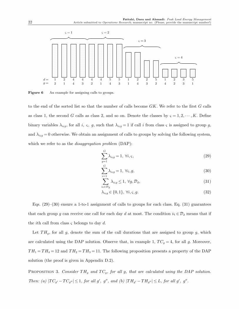
We sort the calls in a non-increasing length order as shown in Fig. 6. The length of a bar shows
the duration of the corresponding call. The first number below the bar indicates the corresponding
day for the call. We divide the calls into classes of size G. This results in 4 classes, which are
denoted by ς = 1,2,3,4. We assign one call from each class to each group. This assignment is always
possible since each class has G calls. An important constraint is that, at most, one call from a day
can be assigned to a group, as without this constraint, the assignment would be straightforward.
In Fig. 6, each group is assigned exactly four calls. The second number below the bar shows the
corresponding group for the call. In the following, we formally state this approach and discuss its
properties.
Assume the AGDP is solved and outputs Dd, for all d, and let D :=⋃D
d=1Dd. Sort the members of
D in a non-increasing length order. If the total number of calls, |D|, is less than GK, add η= (1,0)
Fattahi, Dasu and Ahmadi: Peak Load Energy Management22 Article submitted to Operations Research; manuscript no. (Please, provide the manuscript number!)
d= 1 2 4 4 4 4 5 5 1 2 2 5 1 2 3 5g= 2 1 4 3 2 1 4 3 1 4 3 2 4 2 3 1
ς = 1 ς = 2
ς = 3
ς = 4
Figure 6 An example for assigning calls to groups.
to the end of the sorted list so that the number of calls become GK. We refer to the first G calls
as class 1, the second G calls as class 2, and so on. Denote the classes by ς = 1,2, · · · ,K. Define
binary variables λiςg, for all i, ς, g, such that λiςg = 1 if call i from class ς is assigned to group g,
and λiςg = 0 otherwise. We obtain an assignment of calls to groups by solving the following system,
which we refer to as the disaggregation problem (DAP):
G∑
g=1
λiςg = 1, ∀i, ς, (29)
G∑
i=1
λiςg = 1, ∀ς, g, (30)
∑
iς∈Dd
λiςg ≤ 1, ∀g,Dd, (31)
λiςg ∈ 0,1, ∀i, ς, g. (32)
Eqs. (29)–(30) ensure a 1-to-1 assignment of calls to groups for each class. Eq. (31) guarantees
that each group g can receive one call for each day d at most. The condition iς ∈Dd means that if
the ith call from class ς belongs to day d.
Let THg, for all g, denote the sum of the call durations that are assigned to group g, which
are calculated using the DAP solution. Observe that, in example 1, TCg = 4, for all g. Moreover,
TH1 = TH4 = 12 and TH2 = TH3 = 11. The following proposition presents a property of the DAP
solution (the proof is given in Appendix D.2).
Proposition 3. Consider THg and TCg, for all g, that are calculated using the DAP solution.
Then: (a) |TCg′ −TCg′′ | ≤ 1, for all g′, g′′, and (b) |THg′ −THg′′ | ≤L, for all g′, g′′.

Fattahi, Dasu and Ahmadi: Peak Load Energy ManagementArticle submitted to Operations Research; manuscript no. (Please, provide the manuscript number!) 23
Let Gg, for all g, denote the set of calls that are assigned to group g based on the DAP solution.
Recall that, at most, K calls are assigned to each group because there are K classes. Thus, the
solution satisfies the maximum call per group constraint because |Gg| ≤K for all g.
The total consumption reduction time for group g is THg. We note that the total time per
group constraint may be violated. If THg >H, for some g, we find η ∈ Gg that corresponds to the
minimum saving, and reduce its length. We repeat this process until THg ≤H for all g. The main
steps of our heuristic approach are summarised in Algorithm 4.
Algorithm 4 HGSP heuristic.
1: Solve the ASDP for all (Hd,Kd, ωd) s.t. 0≤Hd ≤GH, 0≤Kd ≤GK, and ωd ∈Ω
2: Solve the AGDP, which results in Dd, for all d
3: Let D :=⋃D
d=1Dd4: Sort the members of D in a non-increasing order of their lengthes
5: Add zeros to the end of the sorted list so that the number of calls become GK
6: Denote the first G calls class 1, the second G calls class 2, and so on
7: Solve the DAP, which results in Gg, for all g
8: for g= 1, · · · ,G do
9: while THg >H do
10: Reduce the length of η ∈ Gg, which corresponds to the least amount of saving
11: end while
12: end for
13: Return Gg, for all g.
Theorem 5. The HGSP always finds a feasible solution to the GDP in a polynomial time.
We next present some results that are used in the proof of theorem 5. We note that the effective-
ness of the HGSP relies heavily on the following issues. First, the DAP must always have a feasible
solution to guarantee that the HGSP can assign calls to groups. Second, the DAP must be solved
in a polynomial time. Let the DAPr denote the LP relaxation of the DAP, which is obtained by
replacing Eq. (32) with 0≤ λiςg ≤ 1, for all i, ς, g.

Fattahi, Dasu and Ahmadi: Peak Load Energy Management24 Article submitted to Operations Research; manuscript no. (Please, provide the manuscript number!)
For a fixed g, let B denote the coefficient matrix for Eq. (30), E1 denote the coefficient matrix
for Eq. (31) with |Dd|= G, and E2 denote the coefficient matrix for Eq. (31) with |Dd|<G. See
Appendix D.3 for a detailed characterization of B, E1, and E2.
Proposition 4. Let Φ := λ ∈ RKG|Bλ = 1K ,E1λ = 1D1,E2λ ≤ 1D2
, λ ≥ 0. Then, Φ is a non-
empty and integral polyhedron.
The proof is given in Appendix D.3. Thus, for a fixed g, one can find an integer solution in Φ in a
polynomial time. In the obtained solution, one call from each class is assigned to g. By eliminating
the assigned calls and group g, the number of groups decreases by 1 while the structure of the
problem is preserved. Hence, by repeating this procedure G times, a feasible solution for the DAP
is found in a polynomial time. Therefore, the proof of theorem 5 is complete.
5.3. Worst-case analysis for the aggregation error
Recall that if THg ≤H, for all g, then the obtained solution is optimal for the GDP; otherwise,
we reduce the duration of some of the calls to achieve THg ≤H, for all g. Let ζsum denote the sum
of the durations of all calls. Proposition 5 states a condition under which the HGSP is guaranteed
to find an optimal solution for the GDP.
Proposition 5. If ζsum ≤G(H −L+ 1), then the HGSP finds an optimal solution for the GDP.
The proof is given in Appendix E.1. If the condition of Proposition 5 does not hold, the HGSP
solution may be infeasible. Recall that if for any g, THg >H, we then reduce the duration of some
of the calls that are assigned to group g.
Next, we prove theorem 4. According to Proposition 3, |TH(n)
g′ − TH(n)
g′′ | ≤ L, for all g′, g′′.
Moreover, one could show, using a contradiction, there exists a group g′ such that TH(n)g ≤ nH.
Hence, by some algebra, we have the following remark.
Remark 3. [TH(n)g −nH]+ ≤L, for all n and g.

Fattahi, Dasu and Ahmadi: Peak Load Energy ManagementArticle submitted to Operations Research; manuscript no. (Please, provide the manuscript number!) 25
Define δ := maxωψAD(1,1, ω); hence, δ is the maximum saving that one could achieve by
assigning a call of length 1 to a group. Therefore, for all n∈Z, n≥ 1, we have:
v(n)AGDP− v(n)HGSP ≤ δ
∑
g
[TH(n)g −nH]+
≤ δGmaxg[TH(n)
g −nH]+
≤ δGL.
This completes the first part of the proof. To prove the second part, note that for any realization
of day-types, we have
v(n)AGDP− v(n)GDP ≤ v
(n)AGDP− v(n)HGSP ≤ δGL,
for all n ∈ Z, n≥ 1, because v(n)HGSP ≤ v(n)GDP. Since this is true for any realization, then E[v
(n)AGSP]−
E[v(n)GSP]≤ δGL, for all n∈Z, n≥ 1. Hence, the proof of theorem 4 is complete.
We next present an alternative approach for the characterization of the aggregation error. Define
the percentage of relative infeasibility as %RI := 100ζsum
∑g [THg −H]
+. Note that if THg ≤H, for
all g, %RI = 0. Moreover, note that although we do not use cost in the definition of %RI, the costs
are considered because the HGSP reduces the duration of calls that are associated with the least
amount of saving.
We present a mathematical model to determine the worse-case %RI for the HGSP. The param-
eters of this model are G, K, H, L∈Z, and we assume they satisfy G≥ 1, K ≥ 1, and H ≥L≥ 2.
Note that the HGSP always finds an optimal solution for the GDP if L = 1. Recall that after
sorting calls, a call is assigned to each group from each class; hence, after the classes are formed,
one can change the order of the calls inside a class. Therefore, the DAP is equivalent to the fol-
lowing problem: change the order of the calls inside the classes such that the following assignment
is feasible: assign the first call from each class to group 1, the second call from each class to group
2, and so on. Let ζiς ∈Z+, for all i, ς, denote the duration of the ith call in class ς. Thus, group g

Fattahi, Dasu and Ahmadi: Peak Load Energy Management26 Article submitted to Operations Research; manuscript no. (Please, provide the manuscript number!)
is assigned ζg1, ζg2, · · · , ζgK and hence THg =∑K
ς=1 ζgς , for all g. Let ζmin,ς , ζmax,ς , for all ς, denote
the minimum and maximum ζiς in class ς. The worst-case %RI problem (WRIP) is as follows:
%WRI = max100
ζsum
G∑
g=1
[(K∑
ς=1
ζgς
)−H
]+(33)
s.t. ζmin,ς ≤ ζiς ≤ ζmax,ς , ∀i, ς, (34)
ζmax,1 ≤L, (35)
ζmin,ς ≥ ζmax,ς+1, ∀ς ≤K − 1, (36)
ζmin,K ≥ 0, (37)
G∑
i=1
K∑
ς=1
ζiς = ζsum, (38)
ζiς , ζmin,ς , ζmax,ς , ζsum ∈R, ∀i, ς. (39)
Eq. (34) ensures that the ζiς is lower bounded by ζmin,ς and upper bounded by ζmax,ς . The first
class includes the largest ζiς , which must be less than or equal to L. This is guaranteed by Eq.
(35). Eq. (36) assures that every call in class ς is at least as big as the maximum duration of the
calls in class ς + 1. Eq. (37) guarantees that the calls in class K have non-negative durations. Eq.
(38) relates the values of ζsum and ζiς .
In the WRIP, we assume ζiς are continuous variables while they must be integers. Hence, one
could assume integral ζiς that may improve the %WRI; however, the WRIP may become more
difficult to solve. A major drawback of the WRIP that makes it very difficult to solve is the
nonlinearity of the objective function. The numerator of the objective function is a piecewise linear
and convex function, and the denominator ζsum is a variable. For a fixed ζsum, one could use
binary variables to convert the WRIP to a MILP problem; however, according to our experiment,
the obtained MILP problem is significantly more difficult. The following proposition presents and
alternative formulation and an effective approach for solving the WRIP in a reasonable time.
Proposition 6. The WRIP is equivalent to the following problem.
%WRI = maxg∗ = 1, · · · ,G,
G(H −L+1)+1≤ ζsum ≤GH.
max 100ζsum
∑g∗
g=1
((∑K
c=1 ζgς
)−H
)
s.t. Eqs. (34)–(39).
(40)
Fattahi, Dasu and Ahmadi: Peak Load Energy ManagementArticle submitted to Operations Research; manuscript no. (Please, provide the manuscript number!) 27
The proof is given in Appendix E.2. We applied Proposition 6 to a real-size problem with G= 20,
K = 100, H = 180, and L= 4, and obtained that the %WRI is 0.56%. Hence, the aggregation error
is significantly small for real-size problems.
6. Computational Experiment
First, we show the quality of our heuristic approach on a set of mid-size problems. Next, we present
the results obtained from applying our heuristic to a real problem which is provided to us by a
large utility company in the Southern California region.
6.1. Error analysis on mid-sized problems
We use the ECPs for a large region of the Southern California from 2012 to 2014. The number of
day-types is set to 5, 10, and 15, and G= 20 and L= 4. We set K = 6n, H = 10n, and D = 20n,
where 1 ≤ n ≤ 5; hence, K varies between 6 and 30, H varies between 10 and 50, and D varies
between 20 and 100. We use a strictly increasing cost function similar to Fig. 1.
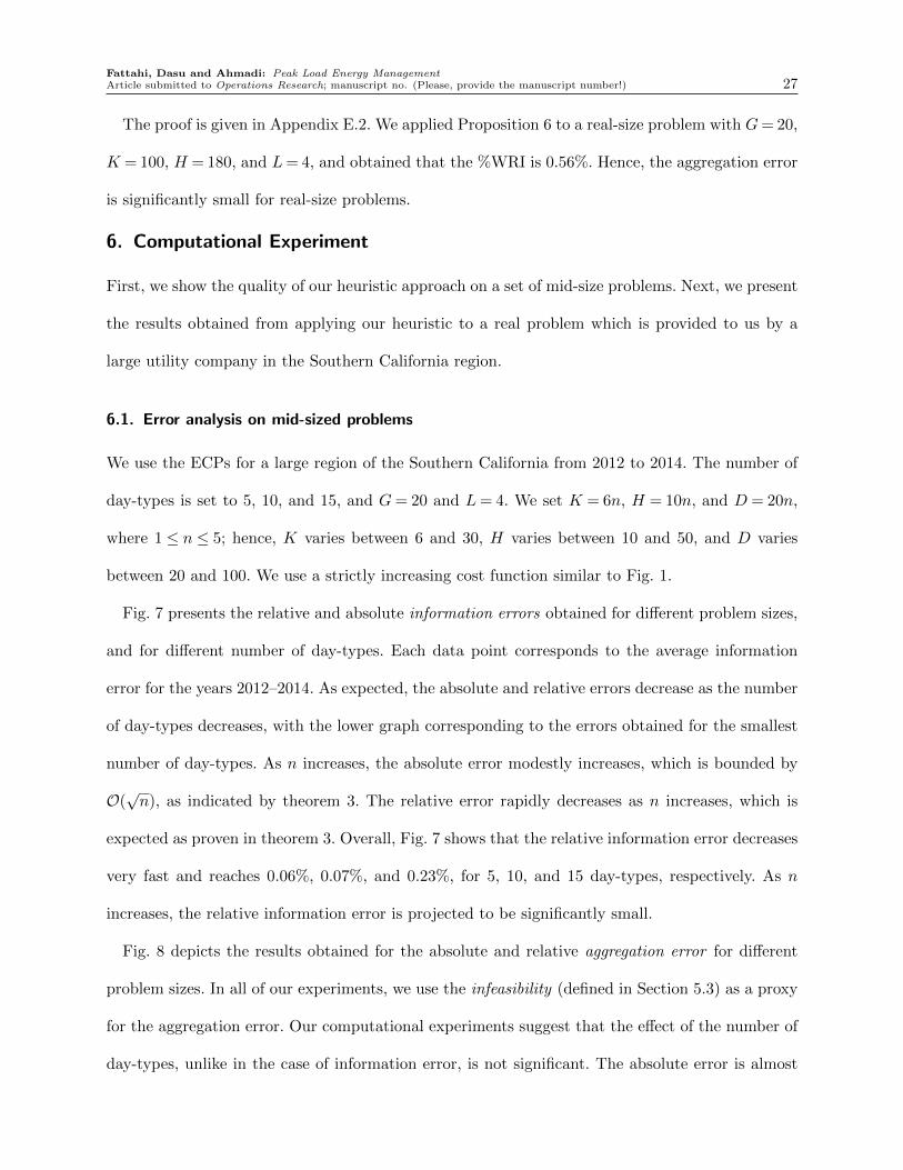
Fig. 7 presents the relative and absolute information errors obtained for different problem sizes,
and for different number of day-types. Each data point corresponds to the average information
error for the years 2012–2014. As expected, the absolute and relative errors decrease as the number
of day-types decreases, with the lower graph corresponding to the errors obtained for the smallest
number of day-types. As n increases, the absolute error modestly increases, which is bounded by
O(√n), as indicated by theorem 3. The relative error rapidly decreases as n increases, which is
expected as proven in theorem 3. Overall, Fig. 7 shows that the relative information error decreases
very fast and reaches 0.06%, 0.07%, and 0.23%, for 5, 10, and 15 day-types, respectively. As n
increases, the relative information error is projected to be significantly small.
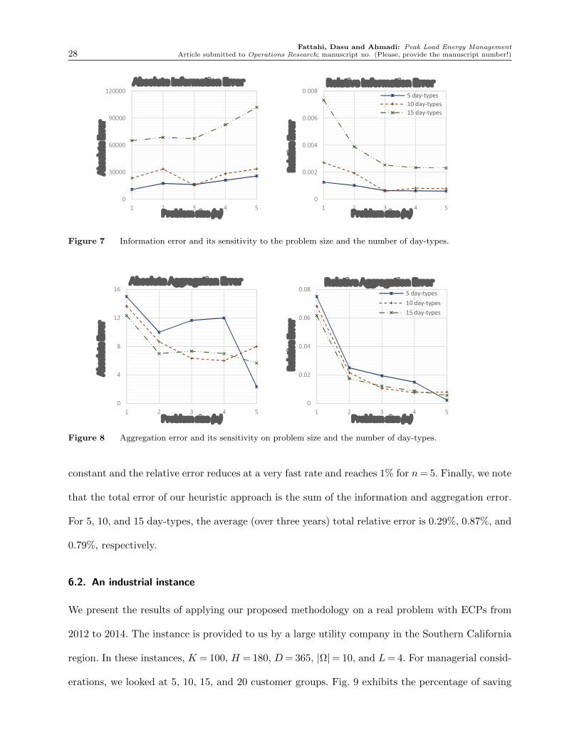
Fig. 8 depicts the results obtained for the absolute and relative aggregation error for different
problem sizes. In all of our experiments, we use the infeasibility (defined in Section 5.3) as a proxy
for the aggregation error. Our computational experiments suggest that the effect of the number of
day-types, unlike in the case of information error, is not significant. The absolute error is almost
Fattahi, Dasu and Ahmadi: Peak Load Energy Management28 Article submitted to Operations Research; manuscript no. (Please, provide the manuscript number!)
0
30000
60000
90000
120000
1 2 3 4 5
Abso
lute
Err
or
Problem size (n)
Absolute Information Error
0
0.002
0.004
0.006
0.008
1 2 3 4 5
Rela
tive
Erro
r
Problem size (n)
Relative Information Error5 day-types10 day-types15 day-types
Figure 7 Information error and its sensitivity to the problem size and the number of day-types.
0
4
8
12
16
1 2 3 4 5
Abso
lute
Err
or
Problem size (n)
Absolute Aggregation Error
0
0.02
0.04
0.06
0.08
1 2 3 4 5
Rela
tive
Erro
r
Problem size (n)
Relative Aggregation Error5 day-types10 day-types15 day-types
Figure 8 Aggregation error and its sensitivity on problem size and the number of day-types.
constant and the relative error reduces at a very fast rate and reaches 1% for n= 5. Finally, we note
that the total error of our heuristic approach is the sum of the information and aggregation error.
For 5, 10, and 15 day-types, the average (over three years) total relative error is 0.29%, 0.87%, and
0.79%, respectively.
6.2. An industrial instance
We present the results of applying our proposed methodology on a real problem with ECPs from
2012 to 2014. The instance is provided to us by a large utility company in the Southern California
region. In these instances, K = 100, H = 180, D= 365, |Ω|= 10, and L= 4. For managerial consid-
erations, we looked at 5, 10, 15, and 20 customer groups. Fig. 9 exhibits the percentage of saving
Fattahi, Dasu and Ahmadi: Peak Load Energy ManagementArticle submitted to Operations Research; manuscript no. (Please, provide the manuscript number!) 29
0.0
2.0
4.0
6.0
8.0
10.0
0 5 10 15 20
% S
avin
g
Number of Groups
Saving in Total Power Cost
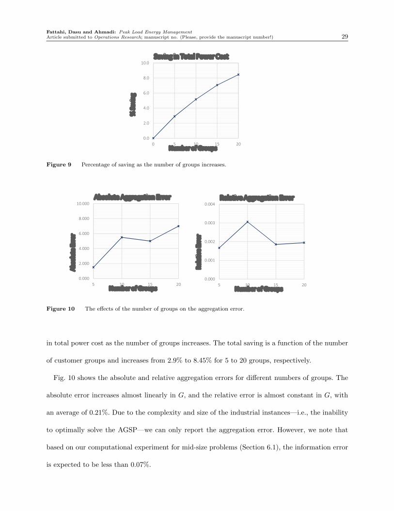
Figure 9 Percentage of saving as the number of groups increases.
0.000
2.000
4.000
6.000
8.000
10.000
5 10 15 20
Abso
lute
Err
or
Number of Groups
Absolute Aggregation Error
0.000
0.001
0.002
0.003
0.004
5 10 15 20
Rela
tive
Erro
r
Number of Groups
Relative Aggregation Error
Figure 10 The effects of the number of groups on the aggregation error.
in total power cost as the number of groups increases. The total saving is a function of the number
of customer groups and increases from 2.9% to 8.45% for 5 to 20 groups, respectively.
Fig. 10 shows the absolute and relative aggregation errors for different numbers of groups. The
absolute error increases almost linearly in G, and the relative error is almost constant in G, with
an average of 0.21%. Due to the complexity and size of the industrial instances—i.e., the inability
to optimally solve the AGSP—we can only report the aggregation error. However, we note that
based on our computational experiment for mid-size problems (Section 6.1), the information error
is expected to be less than 0.07%.

Fattahi, Dasu and Ahmadi: Peak Load Energy Management30 Article submitted to Operations Research; manuscript no. (Please, provide the manuscript number!)
0
5
10
15
20
25
30
35
40
45
3 4 5 7 10
Num
ber o
f Day
s
Number of Groups Called
Frequency distribution of calls
0
5
10
15
20
25
30
35
40
45
9 12 14 17 27 37
Num
ber o
f Day
s
Cumulative Number of Hours Called
Frequency distribution of hours
Figure 11 The frequency distributions of calls and hours.
Our solution scheduled calls for 162 days throughout the year and the frequency distribution of
the daily cumulative calls and hours are shown in Fig. 11. For example, in 35 days, 3 calls per day
are scheduled, and in 20 days, a total of 9 hours per day is assigned to groups.
Finally, we note that the impetus behind DLCCs is to reduce peak load consumption and influ-
ence customers’ energy consumption patterns. Fig. 12 shows the before and after ECP patterns for
the first weeks of winter and summer 2014. In winter, the energy consumption fluctuates between
19 and 29 GW/h, while in summer, it varies between 22 and 36 GW/h. According to our solution,
the summer peak load reduces from 36 to 32 GW/h, which may correspond to a reduction in the
energy production rate from 160 to 80 $/MWh (see Fig. 1).
7. Concluding Remarks
We analyze the problem of efficiently implementing DLCCs used by many utility companies in
developed countries. We optimally solve an special case of the problem in which the lengths of
interventions are equal and fixed. A heuristic approach is proposed based on approximating the
stochasticity, and aggregating the customer groups and forming a representative group. Our heuris-
tic approach is asymptotically optimal and its worst-case relative error is O( 1√n
). The quality of
our heuristic approach under different settings were experimentally verified. An industrial instance
of this problem is thoroughly which results in approximately 8% in the energy generation cost.

Fattahi, Dasu and Ahmadi: Peak Load Energy ManagementArticle submitted to Operations Research; manuscript no. (Please, provide the manuscript number!) 31
15
20
25
30
35
40Winter (January 1-7, 2014)
before
after
Ener
gyCo
nsum
ptio
n Ra
te
(100
0 M
W/H
our)
Ener
gyCo
nsum
ptio
n Ra
te
(100
0 M
W/H
our)
15
20
25
30
35
40Summer (July 1-7, 2014)
Figure 12 The peak load reduction during the first weeks of winter and summer 2014.
Finally, we emphasize that our approach can also be used to efficiently design DLCCs and set
essential contract parameters.
We offer the following directions for future research. First, although we assumed the customer
groups are identical in terms of their demands and contracts, this may not be true in some demand-
response programs. Second, in the DLCCs that were considered in this paper, the peak demand
is eliminated—not shifted—through the scheduled interventions. However, in some programs, in
anticipation of being called for a certain period, a customer group may shift their energy con-
sumption to before and after that period. This phenomenon is referred to as “the shoulder effect”.
Finally, this paper assumes that customers can subscribe to DLCCs only at the beginning of the
planning horizon. However, we note that there are demand-response programs that allow customers
subscribe any time throughout the year. Future research could look at demand-response programs
with non-identical groups, shoulder effects, and/or rolling contracts.

Fattahi, Dasu and Ahmadi: Peak Load Energy Management32 Article submitted to Operations Research; manuscript no. (Please, provide the manuscript number!)
Appendix A: Complexity Proofs
A.1. Proof of Proposition 1(a)
We show that the GDP with G= 2 is as hard as the 2-partition problem, which is known to be
weakly NP-complete (Garey and Johnson 1979). Assume that we are given a general instance of the
2-partition problem consisting of the positive integers α1, α2, . . . , α2D, and A such that∑2D
d=1αd =
2A. The question is: Can α1, α2, . . . , α2D be partitions into two subsets with equal size and equal
number of elements?
Consider the following specific instance of the GDP. Let G= 2 and consider a planning horizon
of 2D days where in day d the height of the ECP is equal to 1 at periods 1, . . . , αd and 0 at periods
αd + 1, . . . , T . Thus, there are 2D ECPs with durations α1, α2, . . . , α2D (see Fig. 13). We assume
T ≥maxd=1,...,2Dαd and L≥maxd=1,...,2Dαd. We assume f(1) = 1 meaning that if we assign αd
to a group, we achieve a saving of αd. Let K =D and H =A.
α1 α2 α2D−1 α2D
1 2 2D− 1 2D
...
days
Figure 13 The ECPs for the planning horizon of 2D days.
Case 1: If the 2-partition has a solution, then the optimal solution of the GDP is obtained by
assigning partitions to groups. The saving that is achieved by this assignment is 2A.
Case 2: If the 2-partition does not have solution, we show that the GDP cannot have a solution
with a total saving of 2A. If the 2-partition does not have solution, then for all partitions with
equal size, there exists Λ> 0 such that the size of the partitions are A−Λ and A+ Λ. Assigning
these partitions to the groups, one could achieve savings of A−Λ and A, respectively. Therefore,
the total saving is 2A−Λ which is strictly less than 2A.
To complete the proof, we note that the GDP with two groups is solved in a pseudo polynomial
time, which implies that the problem is weakly NP-complete.
A.2. Proof of Proposition 1(b)
We show that the GDP is as hard as the 3-partition problem, which is known to be strongly NP-
complete (Garey and Johnson 1979). Assume that we are given a general instance of the 3-partition
problem consisting of positive integers α1, α2, . . . , α3G, and A such that∑3G
d=1αd is divisible by G
and A= 1G
∑3G
d=1αd, and A4≤ αd ≤ A
2, for all d. The question is: Can α1, α2, . . . , α3G be partitioned
into G subsets with equal size and equal number of elements?

Fattahi, Dasu and Ahmadi: Peak Load Energy ManagementArticle submitted to Operations Research; manuscript no. (Please, provide the manuscript number!) 33
Consider the following specific instance of the GDP, with G groups. Let D = 3G, and assume
that the ECP height is 1 in periods 1, . . . , αd and 0 in periods αd + 1, . . . , T , on day d, for all d.
Thus, there are 3G energy consumption periods with durations α1, α2, . . . , α3G. We assume T ≥maxd=1,...,3Gαd and L≥maxd=1,...,3Gαd. We assume f(1) = 1 meaning that if we assign αd to a
group, we achieve a saving of αd. Let K = 3 and H =A.
Case 1: If the 3-partition has a solution, then the optimal solution of the GDP is obtained by
assigning the partitions to groups. The saving that is achieved by this assignment is GA.
Case 2: The 3-partition does not have a solution. Let us partition α1, α2, . . . , α3G intoG subsets with
equal number of elements and assign each set to a group. Hence, each group receives exactly 3 ele-
ments. There exists a positive integer Λ> 0 and groups g′ and g′′ such that∑
d:αd is assigned to g′ αd ≥A+Λ and
∑d:αd is assigned to g′′ αd ≤A−Λ. Therefore, the total saving of this assignment is less than
or equal to GA−Λ and hence is strictly less than GA. Note that this holds for all such partitions
with equal number of elements. Therefore, the optimal solution of the GDP is strictly less than
GA.
Appendix B: FSP Proofs
B.1. Proof of Proposition 2
Let s∗t denote the optimal solution to AFSDPr. If AFSDPr results in a solution in which all s∗t ’s
are integer, then the obtained solution is an optimal solution to AFSDP. Consider the case where
some of the s∗t ’s are fractional. We define, for each t, S∗t :=∑minT−L+1,t
t′=max1,t−L+1 s∗t′ which is the number
of groups who are on call during time period t in the optimal solution. Two or more S∗t ’s must be
fractional. Consider the following linear program (P1).
maxT∑
t=1
∂fd,t(bS∗t c)minT−L+1,t∑
t′=max1,t−L+1st′ , (41)
s.t. Rt ≥ rt(ωd)−minT−L+1,t∑
t′=max1,t−L+1st, ∀t (42)
T−L+1∑
t=1
st =Kd (43)
bS∗t c ≤minT−L+1,t∑
t′=max1,t−L+1st′ ≤ dS∗t e, ∀t, (44)
st ∈R+, ∀t≤ T −L+ 1. (45)
We note that s∗t are feasible for P1. A feasible solution to P1 is also feasible for AFSDPr and
the objective values of AFSDPr and P1 differ by a constant that is independent of st’s. We show
next that all the extreme points of P1 are integer. We note that P1 contains T + 1 constraints

Fattahi, Dasu and Ahmadi: Peak Load Energy Management34 Article submitted to Operations Research; manuscript no. (Please, provide the manuscript number!)
and T −L+ 1 variables. We define ℵt :=∑minT−L+1,t
t′=max1,t−L+1 st′ , for all 1≤ t≤ T . Moreover, we define
ℵ0 :=∑T−L+1
t′=1 st′ , and ℵt := 0, for all t > T .
Assume that T = αL + β, where α is an integer and 0 ≤ β < L. Then, ℵ0 =∑k+1
i=0 ℵj+Li for
j = 1, . . . ,L. Thus constraints corresponding to ℵT−L+1, . . . ,ℵT are redundant constraints. They
are obtained through elementary row operations on the remaining T −L+ 1 constraints. We note
that ℵ0 and ℵ1, . . . ,ℵT are independent of each other as each of them introduces one new variable.
Consider the solution to the following set of equations:
ℵ0 = RHS0 (46)
ℵt = RHSt, ∀t : 1≤ t≤ T −L, (47)
where all the right hand side variables are integers. The solution to this set is easily found, because
ℵ1 = s1, ℵ2 = s1 + s2, and so on. Each constraint introduces exactly one new variable. All the st’s
will be integer.
Any other independent set of T −L+ 1 constraints from the set ℵ0, . . . ,ℵT can be transformed
to the set ℵ0, . . . ,ℵT−L+1 through elementary row operations that does not involve any division,
hence maintaining the integrality of the right hand side. Thus, every extreme point of the polytope
corresponding to P1 is an integer. This implies that there exists a set of integer extreme points
such that their convex combination is s∗, the optimal solution to AFSDPr.
Using property (iii) of the function f , we have, for z′ 6= z′′, ∂fd,t(z′) 6= ∂fd,t(z
′′). Then, if s∗ is
not an extreme point, then there is a strict improvement direction. Hence P1 contains an integer
solution that has a higher objective than that given by s∗. This in turn implies that s∗ is not
optimal to AFSDPr. Thus we proved that AFSDPr yields integer solutions.
B.2. Proof of Lemma 1
We prove this claim using an induction. Before starting the for -loop, we have TCg = 0, for all g.
Assume that in iteration d, we have |TCg′−TCg′′ | ≤ 1, for all g′, g′′. Sort TCg’s in a non-decreasing
order TC[1] ≤ TC[2] ≤ · · · ≤ TC[G]; hence, TC[1] + 1≥ TC[G]. If TC[1] + 1 = TC[G], then there exists
[g] such that TC[1] = · · ·= TC[g]−1 = TC[g]− 1 = · · ·= TC[G]− 1. If TC[1] = TC[G], let [g] = [G] + 1.
Let TC := TC[1]. Then, TC[g] = TC, for all [g] such that [g]< [g], and TC[g] = TC + 1, for all [g]
such that [g]≥ [g].
There exists [g] such that the for -loop assigns a call to each group [g] such that [g] < [g]. Let
[g]min := min[g], [g] and [g]max := max[g], [g]. In iteration d+ 1, we have:
TC[g] =
TC + 1 , ∀[g] : [g]< [g]min
TC , ∀[g] : [g]min ≤ [g]< [g]max, if [g]> [g]
TC + 2 , ∀[g] : [g]min ≤ [g]< [g]max, if [g]< [g]
TC + 1 , ∀[g] : [g]≥ [g]max
Therefore, in iteration d+ 1, we have |TCg′ −TCg′′ | ≤ 1, for all g′, g′′. So, the proof is complete.

Fattahi, Dasu and Ahmadi: Peak Load Energy ManagementArticle submitted to Operations Research; manuscript no. (Please, provide the manuscript number!) 35
B.3. Proof of Lemma 2
According to lemma 1, for d=D− 1, we have |TCg′ −TCg′′ | ≤ 1, for all g′, g′′. Now consider day
D. We assign minKD,G or less but we consider assigning minKD,G because if we can assign
minKD,G to groups, then we can assign smaller values as well. One of the following cases can
happen:
Case 1: KD <G; hence, we assign KD. We claim that in this case each group has at most 1 call
available—i.e., K −TCg ≤ 1, for all g. This claim is proven as follows. Note that at the beginning
of iteration D we have assigned TCg calls to group g, and group g has K − TCg unused calls.
The total unused calls is∑
g(K − TCg) = GK −∑g TCg = KD <G. Assume there exists g such
that K − TCg > 1, then TCg < K − 1. Using Lemma 1, we must have TCg ≤ K − 1, for all g,
with strict inequality for g. Therefore,∑
g TCg <GK−G and hence GK−∑g TCg >G. This is a
contradiction. Thus, each group has at most 1 call available. Therefore, to assign KD, we call each
group g with an available call.
Case 2: KD ≥G; hence, we assign G. We claim that in this case each group has at least 1 call
available—i.e., K − TCg ≥ 1, for all g. We prove this claim by contradiction. Assume there exists
g such that K−TCg < 1. Then, TCg >K− 1. Using Lemma 1, we must have TCg ≥K− 1, for all
g, with strict inequality for g. Therefore,∑
g TCg >GK −G and hence KD =GK −∑g TCg <G.
This is a contradiction. Thus, each group has at least 1 call available. Therefore, to assign G calls,
we call all groups.
Appendix C: Information Error Proofs
C.1. Proof of Lemma 3
We prove the following relationship, for all n∈Z, n≥ 1, which proves the lemma.
E[v(n)UBH] = v
(n)RAGDP ≥ v(n)AGDP ≥E[v
(n)AGSP]≥E[v
(n)LBH].
Note that E[v(n)UBH] =
∑nD
d=1
∑j qjpω(j)θj =
∑j
∑nD
d=1
x∗jDθj = n
∑j θjx
∗j = v
(n)RAGDP, for all n∈Z, n≥
1. Because RAGDP(n) is a relaxation of AGDP(n), then v(n)RAGDP ≥ v(n)AGDP, for all n ∈ Z, n ≥ 1.
Recall that in AGDP(n) we assume that npωD days are from type ω, for all ω. Also, recall that
we assume pωD is integer for all ω. Note that the optimal value of AGDP(n) is concave in the
number of days of type ω, for all ω. Also, using Jensen’s inequality, we have v(n)AGDP ≥E[v
(n)AGSP], for
all n∈Z, n≥ 1. Because LBH(n) provides a feasible solution to AGSP(n), then E[v(n)AGSP]≥E[v
(n)LBH],
for all n∈Z, n≥ 1.

Fattahi, Dasu and Ahmadi: Peak Load Energy Management36 Article submitted to Operations Research; manuscript no. (Please, provide the manuscript number!)
C.2. Proof of Lemma 4
For all γ and d, we have:
E[(∆(n)γ (d))2|=d] =
∑
j
pω(j)qj(aγj −
∑
j′
pω(j′)qj′aγj′)2 ≤ 1
4a2γ,max.
This inequality follows from Popoviciu’s inequality according to which V ar(x)≤ 14(x−x)2, where
x ≤ x ≤ x with probability 1. We note that∑
j pω(j)qj(aγj −∑
j′ pω(j′)qj′aγj′)2 is the variance of
aγ1, . . . , aγJ . Also note that for all j, 0≤ aγj ≤ aγ,max. Hence, the variance does not exceed 14a2γ,max.
To complete the proof, we note that E[(∑d
d′=1 ∆(n)γ (d′))2|=d] =
∑d
d′=1 E[(∆(n)γ (d′))2|=d′ ] because
considering the filtration =d, the error terms, ∆(n)γ (d′), are independent.
C.3. Proof of Lemma 5
The probability P (d∗(n) < d) is found by calculating the probability of the violation of condition
(†) for some resource γ and for some days d < d. Therefore, we have:
P (d∗(n) <d) = P( d∑
d′=1
∆(n)γ (d′)>ncγ −
d
Daγx
∗− aγ,max, for some γ, d < d)
≤∑
γ
P( d∑
d′=1
∆(n)γ (d′)>ncγ −
d
Daγx
∗− aγ,max, for some d≤ d)
Since, d≤ d, we replace d with d in the right-hand-side of the condition; hence, the right-hand-side
becomes a constant (independent of d). Therefore, we can take the maximum of∑d
d′=1 ∆(n)γ (d′)
over d= 1, . . . , d, and hence we have:
P (d∗(n) <d) ≤∑
γ
P(
maxd=1,...,d
d∑
d′=1
∆(n)γ (d′)>ncγ −
d
Daγx
∗− aγ,max
)
≤∑
γ
P(
maxd=1,...,d
∣∣d∑
d′=1
∆(n)γ (d′)
∣∣≥ n(cγ −
d
nDaγx
∗)− aγ,max
)
≤∑
γ
E[(∑d
d′=1 ∆(n)γ (d′)
)2](n(cγ − d
nDaγx∗)− aγ,max
)2 (48)
≤∑
γ
d( 2n
aγ,max
(cγ −d
nDaγx
∗)− 2)−2
(49)
Inequality (48) follows from Doob’s submartingale inequality, and inequality (49) follows from
applying Lemma 4. To complete the proof, we note that P (d∗(n) <d)≤ 1, for all n and d.
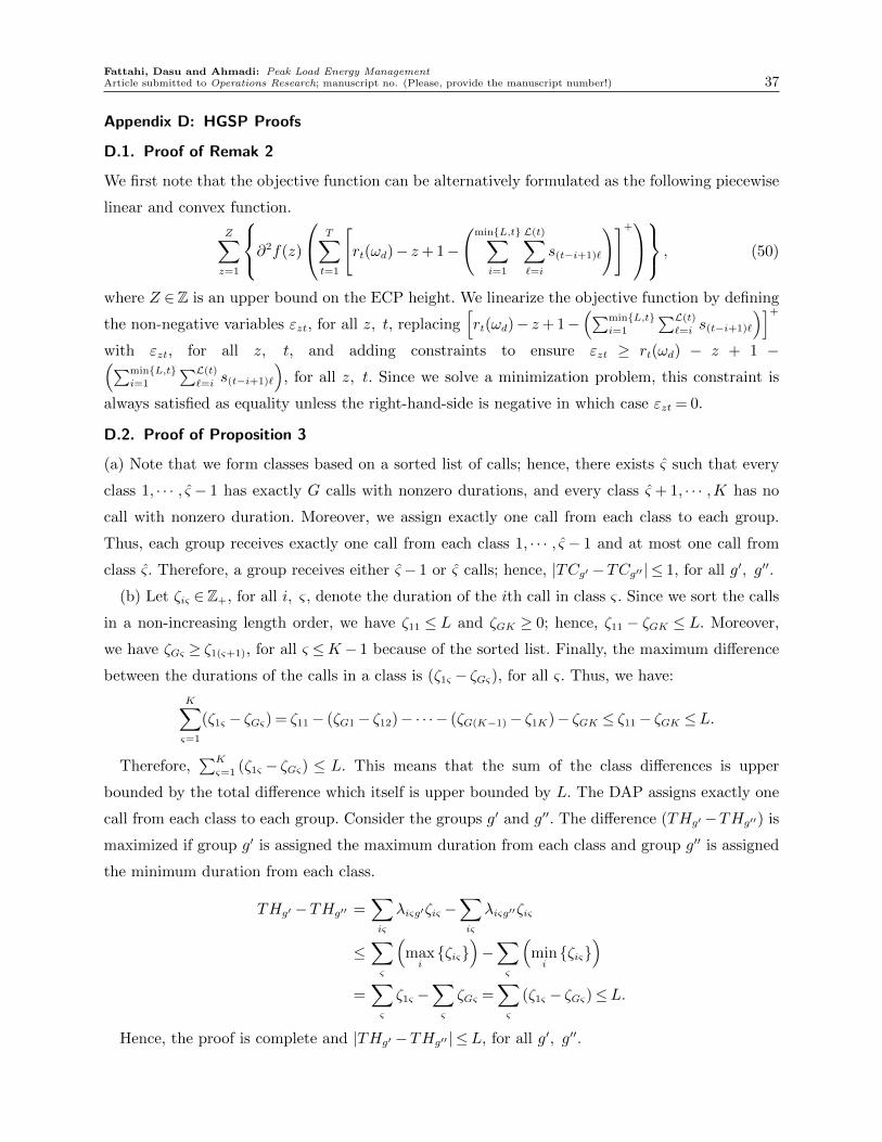
Fattahi, Dasu and Ahmadi: Peak Load Energy ManagementArticle submitted to Operations Research; manuscript no. (Please, provide the manuscript number!) 37
Appendix D: HGSP Proofs
D.1. Proof of Remak 2
We first note that the objective function can be alternatively formulated as the following piecewise
linear and convex function.
Z∑
z=1
∂
2f(z)
T∑
t=1
[rt(ωd)− z+ 1−
(minL,t∑
i=1
L(t)∑
`=i
s(t−i+1)`
)]+ , (50)
where Z ∈Z is an upper bound on the ECP height. We linearize the objective function by defining
the non-negative variables εzt, for all z, t, replacing[rt(ωd)− z+ 1−
(∑minL,ti=1
∑L(t)`=i s(t−i+1)`
)]+
with εzt, for all z, t, and adding constraints to ensure εzt ≥ rt(ωd) − z + 1 −(∑minL,ti=1
∑L(t)`=i s(t−i+1)`
), for all z, t. Since we solve a minimization problem, this constraint is
always satisfied as equality unless the right-hand-side is negative in which case εzt = 0.
D.2. Proof of Proposition 3
(a) Note that we form classes based on a sorted list of calls; hence, there exists ς such that every
class 1, · · · , ς − 1 has exactly G calls with nonzero durations, and every class ς + 1, · · · ,K has no
call with nonzero duration. Moreover, we assign exactly one call from each class to each group.
Thus, each group receives exactly one call from each class 1, · · · , ς − 1 and at most one call from
class ς. Therefore, a group receives either ς − 1 or ς calls; hence, |TCg′ −TCg′′ | ≤ 1, for all g′, g′′.
(b) Let ζiς ∈Z+, for all i, ς, denote the duration of the ith call in class ς. Since we sort the calls
in a non-increasing length order, we have ζ11 ≤ L and ζGK ≥ 0; hence, ζ11 − ζGK ≤ L. Moreover,
we have ζGς ≥ ζ1(ς+1), for all ς ≤K − 1 because of the sorted list. Finally, the maximum difference
between the durations of the calls in a class is (ζ1ς − ζGς), for all ς. Thus, we have:
K∑
ς=1
(ζ1ς − ζGς) = ζ11− (ζG1− ζ12)− · · ·− (ζG(K−1)− ζ1K)− ζGK ≤ ζ11− ζGK ≤L.
Therefore,∑K
ς=1 (ζ1ς − ζGς) ≤ L. This means that the sum of the class differences is upper
bounded by the total difference which itself is upper bounded by L. The DAP assigns exactly one
call from each class to each group. Consider the groups g′ and g′′. The difference (THg′ −THg′′) is
maximized if group g′ is assigned the maximum duration from each class and group g′′ is assigned
the minimum duration from each class.
THg′ −THg′′ =∑
iς
λiςg′ζiς −∑
iς
λiςg′′ζiς
≤∑
ς
(maxiζiς
)−∑
ς
(miniζiς
)
=∑
ς
ζ1ς −∑
ς
ζGς =∑
ς
(ζ1ς − ζGς)≤L.
Hence, the proof is complete and |THg′ −THg′′ | ≤L, for all g′, g′′.

Fattahi, Dasu and Ahmadi: Peak Load Energy Management38 Article submitted to Operations Research; manuscript no. (Please, provide the manuscript number!)
D.3. Proof of Proposition 4
Adding slack variables to Eq. (31), the DAPr is equivalent to the following system of equations.
G∑
g=1
λiςg = 1, ∀i, ς, (51)
G∑
i=1
λiςg = 1, ∀ς, g, (52)
∑
iς∈Dd
λiςg +σgd = 1, ∀g,Dd, (53)
where, λiςg, for all i, ς, g, and σgd, for all g, d, are non-negative continuous variables. We note
that λiςg cannot take a value greater than 1 because the right-hand-side values are 1, all of the
coefficients in the left-hand-sides are 1, and all variables are non-negative and continuous. Thus,
constraint λiςg ≤ 1, for all i, ς, g, is automatically ensured. Thus, the coefficient matrix of DAPr
is a (2KG+DG)× (KG2 +DG)-matrix of zeros and ones as follows.
A=
IKG IKG · · · IKG 0B 0 · · · 0 00 B · · · 0 0...
.... . .
... 00 0 · · · B 0E 0 · · · 00 E · · · 0 IDG...
.... . .
...0 0 · · · E
, BK×KG =
1′G 0 · · · 0
0 1′G · · · 0
......
. . ....
0 0 · · · 1′G
,
and E is a (D×KG)-matrix of zeros and ones. The following remark states that the matrix A has
(DG+ 2KG−K) linearly independent rows and columns. The proof is standard and follows from
performing some elementary operations on A.
Remark 4. The rank of matrix A is (DG+ 2KG−K).
It is seen that B is a matrix of zeros and ones. Each column of B has exactly one 1 and exactly
(K−1) zeros. Moreover, each row of B has exactly G ones and exactly (K−1)G zeros. We similarly
characterize the columns and rows of E in the following remark. The proof is standard and follows
from analyzing Eq. (53).
Remark 5. Matrix E has the following properties: (i) each entry is either 0 or 1, (ii) each column
has exactly one 1, and (iii) each row has at most G ones. Moreover, if D=K, then each row of Ehas exactly G ones.
We partition E into two sub-matrices as follows: E1 consists of the rows of E that have exactly G
ones, and E2 consists of the rows of E that have strictly less than G ones. Let Φ := λ∈RKG|Bλ=
Fattahi, Dasu and Ahmadi: Peak Load Energy ManagementArticle submitted to Operations Research; manuscript no. (Please, provide the manuscript number!) 39
1K ,E1λ = 1D1,E2λ ≤ 1D2
, λ ≥ 0. In the following, we show that Φ is a nonempty and integral
polyhedron.
Adding slack variables to E2λ ≤ 1D2, the coefficient matrix becomes
B 0E1 0E2 ID2
and the right-
hand-side vector is 1(K+D). Recall that each column of B and E has exactly one 1 (see Remark 5);
hence, each column of the coefficient matrix has at most 2 ones. Additionally, if there are 2 ones
in a column of the coefficient matrix, one of them is in the first K rows and the other one is in the
last D rows. Therefore, the coefficient matrix is totally unimodular meaning that every extreme
point of the feasible region is integral and thus the set Φ is an integral polyhedron.
We next prove that Φ is nonempty. Consider the following LP problem: max 0 s.t. λ ∈ Φ. The
dual problem is as follows.
min 1′
Gχ1 + 1′
D1χ2 + 1
′
D2χ3 (54)
s.t.
BE1E2
′ χ1χ2χ3
≥ 0 (55)
χ3≥ 0, (56)
where, χ1, χ2, χ3 are the dual variables. One could see that the dual problem is feasible because
χ1 = 0, χ2 = 0, and χ3 = 0 satisfy the constraints. We need to show that the optimal value for the
dual problem is finite. Consider the relaxation of the dual problem that is obtained by multiplying
Eq. (55) by 1′K+D from the left. This results in the following inequality.
G1KG1D1
ℵ
′ χ1χ2χ3
≥ 0 (57)
where, ℵ ∈RD2 and ℵ ≤G1D2. Thus, the relaxation of the dual problem includes Eqs. (54), (56),
and (57). Note that every feasible solution to the dual problem is also feasible for the relaxation
problem but the converse may not be true. Eq. (57) can be written as follows.
G1′
Kχ1 +G1′
D1χ2 +ℵ′χ3≥ 0
=⇒G(1′
Kχ1 + 1′
D1χ2 + 1
′
D2χ3)−(G1
′
D2χ3−ℵ′χ3
)≥ 0
=⇒ 1′
Kχ1 + 1′
D1χ2 + 1
′
D2χ3≥ 1
G
(G1D2
−ℵ)′χ3
=⇒ 1′
Kχ1 + 1′
D1χ2 + 1
′
D2χ3≥ 0
Thus, the optimal value of the relaxation of the dual problem is bounded below; hence, the
optimal value of the dual problem is bounded. Therefore, since the dual problem has a finite optimal
solution, then the primal problem also has a solution. Thus, we proved that Φ is nonempty.
Fattahi, Dasu and Ahmadi: Peak Load Energy Management40 Article submitted to Operations Research; manuscript no. (Please, provide the manuscript number!)
Appendix E: Aggregation Error Proofs
E.1. Proof of Proposition 5
We show that if ζsum ≤G(H −L+ 1), then THg ≤H, for all g. We use a contradiction as follows.
Assume ζsum ≤G(H −L+ 1) and there exists g′ such that THg′ ≥H + 1. Using Proposition 3(b),
we must have THg ≥H−L+1, for all g. Note that if there exists g′′ such that THg′′ ≤H−L, then
THg′−THg′′ ≥L+1 which contradicts Proposition 3(b). Hence, we showed that THg ≥H−L+1,
for all g. Then, ζsum =∑
g THg >G(H−L+1) which contradicts our earlier assumption. Therefore,
THg ≤H, for all g.
E.2. Proof of Proposition 6
Consider G(H−L+ 1) + 1≤ ζsum ≤GH. We first show that this interval is nonempty if L≥ 2. We
have:
1≤ ζsum−G(H −L+ 1)≤G(L− 1)
The right-hand-side is lower bounded by G. If G= 1, we have at least one feasible point. There-
fore, the interval for ζsum is always nonempty. Using Proposition 5, if ζsum ≤G(H −L+ 1), then
the HGSP solution is optimal and hence %RI = 0. Thus, the optimal value of ζsum must satisfy
G(H − L + 1) + 1 ≤ ζsum ≤ GH. Moreover, since this interval is nonempty and %RI is always
non-negative, we can limit our search to this interval.
Let us fix ζsum and focus on maximizing the numerator of the objective function. We note that,
for some groups, we have THg >H, and for the remaining groups we have THg ≤H. Thus, we can
assume that the groups with THg >H are located first in the list. Therefore, there must exist an
optimal solution that satisfies the following condition: there exists g∗ such that THg >H for all
g≤ g∗ and THg ≤H for all g > g∗. Thus, we can limit our search to finding the optimal g∗.
Appendix F: Notations
Abbreviations:AFSDP Aggregate fixed-length single day problemAFSDP∗ An alternative formulation for the AFSDPAFSDPr The linear programming relaxation of the AFSDP∗
AFSP Aggregate fixed-length stochastic problemAGDP Aggregate general deterministic problemAGSP Aggregate general stochastic problemASDP Aggregate single day problemASDP∗ An alternative formulation for the ASDPDAP Disaggregation problemDAPr The LP relaxation of the DAPDLCC Direct load control contract

Fattahi, Dasu and Ahmadi: Peak Load Energy ManagementArticle submitted to Operations Research; manuscript no. (Please, provide the manuscript number!) 41
DP Dynamic programmingECP Energy consumption profileFLP Fixed-length policyFSP Fixed-length stochastic problemGDP General deterministic problemGSP General stochastic problemHGSP Our heuristic approach for solving the GSPLBH Lower-bound heuristicLP Linear programmingMILP Mixed-integer linear programmingRAGDP The LP relaxation of the AGDPSDP Single day problemUBH Upper-bound heuristicWRIP worst-case %RI problem
Notations:g= 1, . . . ,G Groups.d= 1, . . . ,D Days.t= 1, . . . , T Time periods in a day.ω ∈Ω Day-types.ωd Type of day d.ldg Duration of the call for group g in day d.mdg 1, if group g reduces their consumption in day d (if ldg > 0), and 0 otherwise.hdg Remaining hours that group g can reduce their consumption in days d, . . . ,D.kdg Remaining number of times that group g can be called in days d, . . . ,D.Ld Vector Ld = (ld1, . . . , ldG)Md Vector Md = (md1, . . . ,mdG)Hd Vector Hd = (hd1, . . . , hdG)Kd Vector Kd = (kd1, . . . , kdG)L Upper bound on the duration of a call.H Upper bound on the total duration of the calls for a group in the entire horizon.K Upper bound on the number of the calls for a group in the entire horizon.Θd The set of feasible decisions (Ld,Md) on day d.Θfd The set of feasible decisions under FLP on day d.
Θafd The set of feasible decisions for the AFSP on day d.
Θadd The set of feasible decisions for the AGDP on day d.
I(.) The indicator function, i.e., I(z) = 1 if z > 0 and otherwise I(z) = 0.Vd(Hd,Kd) The optimal cost for days d, d+ 1, . . . ,D given Hd available time and Kd avail-
able number of calls to groups.Vfd(Kd) The optimal cost for days d, d+ 1, . . . ,D under FLP, given Kd available calls.Vafd (Kd) The optimal cost for days d, d+1, . . . ,D for AFSP, given a total of Kd available
calls.Vadd (Hd,Kd) The optimal cost for days d, d+ 1, . . . ,D for the AGDP, given a total of Hd
available hours and Kd available calls.ψ(Ld, ωd) The minimum cost for day d of type ωd using the calls Ld = (ld1, . . . , ldG).ψaf(Kd, ωd) The minimum cost for AFSDP for day d of type ωd using Kd calls.ψad(Hd,Kd, ωd) The minimum cost for the ASDP on day d of type ωd using Hd hours and Kd
calls.rt(ωd) The height of ECP in period t and day d.f(.) Energy cost function.
Fattahi, Dasu and Ahmadi: Peak Load Energy Management42 Article submitted to Operations Research; manuscript no. (Please, provide the manuscript number!)
fd,t(.) Energy saving function at period t of day d. Note: fd,t(z) measures the savingat period t of day d given that the height of the ECP has reduced to z.
∂f(.) The first difference of function f , i.e., ∂f(z) := f(z)− f(z− 1), z ∈Z, z ≥ 1.∂2f(.) The second difference of function f , i.e., ∂2f(z) := ∂f(z)−∂f(z−1), z ∈Z, z ≥
1.ugt 1 if group g is on call in period t of day d, and 0 otherwise.wgt 1 if group g begins reducing their consumption in period t of day d, and 0
otherwise.[.]+ The function that is defined as [z]+ := maxz,0.Kd The total number of calls to be used in day d.Hd The total hours to be used in day d.Kd The number of available calls that can be used in days d, d+ 1, · · · ,D.Hd The available hours that can be used in days d, d+ 1, · · · ,D.st The number of groups that start reducing their energy consumption at period
t in day d.st` The number of calls with duration ` and starting time t.Rt The height of the ECP at period t of day d after the customers reduce their
energy consumption.Dd The set of calls that we must use in day d based on the optimal solution of
AFSP.
D Defined as D :=⋃D
d=1Dd.TCg The total number of calls to group g in the entire planning horizon.THg The sum of the call durations that are assigned to group g in the entire planning
horizon.n problem size, n∈Z, n≥ 1.
v(n)GSP The optimal saving for the GSP where the problem size is n.
v(n)HGSP The HGSP saving where the problem size is n.
v(n)AGDP The optimal saving for the AGDP where the problem size is n.
v(n)AGSP The optimal saving for the AGSP where the problem size is n.
v(n)RAGDP The optimal saving for the RAGDP where the problem size is n.ρ A non-negative constant, independent of n, as the upper bound on the aggre-
gation error.j = 1, . . . , J Offers.qj The allocation probability for offer j.xj The number of times that offer j is made in the planning horizon.
x∗(n) The vector (x∗1(n), . . . , x∗J
(n)) and the optimal solution of the RAGDP(n).γ = 1, . . . ,Γ Resources.aγj The amount of resource γ used when offer j is made.cγ The total available resource γ at the beginning of the planning horizon.aγ The vector (aγ1, . . . , aγJ).aγ,max Defined as maxjaγj for all γ.θj The saving from offer j.θmax Defined as θmax := maxjθj.ω(j) The day-type in which offer j can be used.pω The proportion of days of type ω (the probability of day-type ω).
d∗(n) The minimum of nD and the last day in which the condition (†) is satisfied.∆(n)γ (d) The deviation from the expected resource usage for γ on day d.=d The accumulated information up to day d.E[.] The expected value function.P (.) The probability function.

Fattahi, Dasu and Ahmadi: Peak Load Energy ManagementArticle submitted to Operations Research; manuscript no. (Please, provide the manuscript number!) 43
|.| The cardinality/absolute value function.d.e The ceiling function.L(t) Defined as L(t) := minL,T − t+ 1 which denotes the maximum duration of
a call starting from t.st` The number of calls with duration ` and starting time t.η ∈Dd Calls that are scheduled on day d. A call is in the form of η= (st(η), |η|) where
st(η)∈Z+ is the starting time and |η| ∈Z+ is the length of the call.ς = 1, . . . ,K Classes.λiςg 1 if call i from class ς is assigned to group g, and 0 otherwise.Gg The set of calls that are assigned to group g.B, E1, E2 The coefficient matrices for the DAP.Φ Defined as Φ := λ∈RKG|Bλ= 1K ,E1λ= 1D1
,E2λ≤ 1D2, λ≥ 0.
ζsum The sum of the durations of all calls.δ Defined as δ := maxωψAD(1,1, ω).ζiς The duration of the ith call in class ς.ζmin,ς , ζmax,ς The minimum and maximum ζiς in class ς.%RI Percentage of relative infeasibility%WRI Worst-case for %RI
Acknowledgement
The authors at UCLA would like to thank the UCLA Ziman Center for Real Estates UCLA Ziman
Centers Howard and Irene Levine Program in Housing and Social Responsibility for generous
funding.
Endnotes
1. http://www.sandc.com/en/outages#Solutions
2. http://www.popularmechanics.com/science/energy/a6013/how-a-smarter-grid-can-prevent-
blackouts/
3. Creating identical groups may be somewhat difficult in some situations; however, according to
the energy company we are working with, it is common to assume there are identical groups with
the same contracts and power consumption.
References
Adelman D (2007) Dynamic bid prices in revenue management. Operations Research 55(4):647-661.
Alizamir S, de Vericourt F, Sun P (2016) Efficient feed-in-tariff policies for renewable energy technologies.
Operations Research 64(1):52-66.
Baldick R, Kolos S, Tompaidis S (2006) Interruptible electricity contracts from an electricity retailer’s point
of view: valuation and optimal interruption. Operations Research 54(4):627-642.

Fattahi, Dasu and Ahmadi: Peak Load Energy Management44 Article submitted to Operations Research; manuscript no. (Please, provide the manuscript number!)
California Independent System Operator (2012) www.caiso.com.
Cooper WL (2002) Asymptotic behavior of an allocation policy for revenue management. Operations Research
50(4):720-727.
Garey MR, Johnson DS (1979) Computers and Intractability: A Guide to the Theory of NP-Completeness.
WH Freeman & Co., San Francisco.
Jasin S, Kumar S (2012) A re-solving heuristic with bounded revenue loss for network revenue management
with customer choice. Mathematics of Operations Research 37(2):313-345.
Kamat R, Oren SS (2002) Exotic options for interruptible electricity supply contracts. Operations Research
50(5):835-850.
Meulemeester BD (2014) Capacity payments: expensive solution for a non-existing problem. http://
energypost.eu/capacity-payments-expensive-solution-non-existing-problem/.
Michigan Public Service Commission (2015) Common Demand Response Practices and Program Designs.
https://www.michigan.gov/documents/energy/Common_Practices_Feb22_522983_7.pdf.
Next-Kraftwerke-Belgium (2016) Merit order curve. https://www.next-kraftwerke.be/
Oren SS, Smith SA (1992) Design and management of curtailable electricity service to reduce annual peaks.
Operations Research 40(2):213-228.
Peura H, Bunn DW (2015) Dynamic Pricing of Peak Production. Operations Research 63(6):1262-1279.
Posner B (2015) The Fundamentals of Electricity Markets. https://www.e-education.psu.edu/ebf200wd/
node/151
Solar Energy Industries Association (2016) www.seia.org.
Taylor B, Taylor C (2015) Demand Response: Managing Electric Power Peak Load Short-
ages with Market Mechanisms. http://www.raponline.org/wp-content/uploads/2016/05/
rap-china-demandresponsemanagingpeakloadshortages-2015-mar.pdf.
Zhang D, Adelman D (2009) An approximate dynamic programming approach to network revenue manage-
ment with customer choice. Transportation Science 43(3):381394.