Peak of the day - internship at Deep BlueCapital

Nout Jan Dogterom

June 10, 2016

Bachelor thesis

Supervisor: dr. Robin de Vilderdr. Asma Khedher

Victor Harmsen, MSc

Korteweg-de Vries Instituut voor Wiskunde

Faculteit der Natuurwetenschappen, Wiskunde en Informatica

Universiteit van Amsterdam

Abstract

For this thesis, an internship was followed at Deep Blue Capital. Here, events of stocksexceeding their daily maximum up to that point were investigated with the goal ofdevising a trading strategy based on such events. Additional demands on the eventsyielded promising trading strategies. Alongside, the occurence of events and the per-formance of the algorithm following events were compared between historical data anddata generated according to theoretical models.

Title: Peak of the day - internship at Deep Blue CapitalAuthor: Nout Jan Dogterom, noutjan.dogterom@student.uva.nl, 10386580Supervisor: dr. Robin de Vilderdr. Asma KhedherVictor Harmsen, MScDate: June 10, 2016

Korteweg-de Vries Instituut voor WiskundeUniversiteit van AmsterdamScience Park 904, 1098 XH Amsterdamhttp://www.science.uva.nl/math

2

Contents

1. Introduction 41.1. Stock trading . . . . . . . . . . . . . . . . . . . . . . . . . . . . . . . . . 41.2. My internship . . . . . . . . . . . . . . . . . . . . . . . . . . . . . . . . . 5

2. Mathematical framework of trading 62.1. Background and framework concepts . . . . . . . . . . . . . . . . . . . . 62.2. Data dredging and how not to . . . . . . . . . . . . . . . . . . . . . . . . 92.3. Mathematical models for stock price returns . . . . . . . . . . . . . . . . 10

3. Algorithm and performance analysis 143.1. My first algorithm . . . . . . . . . . . . . . . . . . . . . . . . . . . . . . 143.2. Historical sample data performance . . . . . . . . . . . . . . . . . . . . . 153.3. Theoretical sample data performance . . . . . . . . . . . . . . . . . . . . 21

4. Conclusion 25

5. Popular summary 26

Bibliografie 28

A. Internship 29

B. Matlab code 38

3

1. Introduction

This chapter includes the general subject, some background and my motivation.

1.1. Stock trading

Stocks have been around for ages, and ever since they have been they have offered allsorts of monetary opportunities waiting for speculators to take them. Ever since itsconception, this practice has involved statistics. After all, history has shown us timeand time again that we never know for sure what’ll happen next. Uncertainty is certainlyinvolved.

Historically however, stocks and derivatives trading always remained an inherentlyhuman process: every trade required two parties to agree. Many qualities besides statis-tical rigor could lead to great success (and, obviously, bankruptcy). An outsider mightstill equate stock day trading with men shouting frantically through telephones. Thesemen are a dying breed.

Subsequent and ongoing inventions and improvements of computers, the internet and(big) data analysis have only very recently combined to allow for a new framework inwhich stocks may be traded: via computers executing orders without direct humanintervention. This algorithmic approach has clear benefits. A computer can keep trackof many more time series much more accurately than any human ever could. Theyrequire no reimbursement and can work day and night. And, importantly, armed withthe right statistical knowledge it may make many more, much more calculated choicesthan the shouting men ever could.

The floors no longer flooded. Source: [1]

4

1.2. My internship

The practice of letting a superiorly programmed computer invade a human game withsuch high potential payoff has fascinated me since from well back into my childhood.As the focus in this area lies strongly on quantitive analysis and programming, it inpart fueled my choice for a mathematics bachelor. During an internship at Deep BlueCapital, a trading company owned in part by my internship supervisor Robin de Vilder,I could work on the subject myself for the first time.

The internship consisted of approximately 30 days of full time office work. The overallgoal was to try to create a viable trading algorithm, and compare its results betweenactual data and data generated from theoretical models. Reflection with Robin andVictor Harmsen during an introductory talk yielded a topic to be investigated. Considerthe time series of intraday prices of a stock. What might we expect to happen afterthe stock attains its highest daily value so far? It might stray from its short-term meaneven more or gradually fall back, displaying mean-reversing behaviour. There might bea certain degree of predictability involved in the stock’s price following one such event,as we know short-term mean reversion is often present in financial data.

My goal was to find further conditions, under which stocks display a statisticallysignificant degree of predictability. This could lead to insight in supply and demandof a stock, and in short-term future prices of the stock. This in turn might lead toa (profitable) trading strategy centered around extrema breaches. Alongside, eventoccurence was compared between real life financial data and some time series modelsused to analyze or predict real life data.

5

2. Mathematical framework oftrading

Before a high-level description of the research can be given, it is useful to introduce someof the concepts involved. The first section focusses on the ideas and data manipulationsused in the processing of the data used and by the algorithm. Some attention is paidto data dredging in the second section. The third section treats several theoretical timeseries models sometimes used to model or generate financial data.

2.1. Background and framework concepts

The main goal of the internship was to create a Trading algorithm, an algorithm specify-ing how to trade stocks. An algorithm is broadly defined as a fixed set of steps translatingsome input into some output. A cooking recipe provides an intuitive example fit for anyparent to understand. After programming the idea into a script a computer may executeit and, in this case, trade the way a human might.

Trading algorithms may use current, as well as past, stock prices and trade volumes.These are organised in so-called time series, countable sets of sequentially observed data,in this case stock prices at specified times. They are of the form zt = {z0, z1, . . . }. Notethe time series convention of denoting the whole series by zt, not z.

During the internship, raw data came in the form of two kinds of time series: interdaydata with one value specified for every day, whereas in intraday data the fluctuationoccuring during a day is specified (say, one price for each minute). In time series analysisa certain stock y’s price interday time series as a whole is denoted as yt, and its intradaytime series is denoted as yt. Within the series set t, usually an integer, takes valuescorresponding to the time of day in some form. For example, the amount of minutespast 8 a.m. may be the number used. Intraday time series are denoted yt, and (first)differences ∆yt = yt − yt−1.

Simultaneously, we may regard the movement of a stock y’s price as a stochastic pro-cess, denoted also by y = (δt)t∈{1,...,n}. Stock prices may also be regarded as continuous-time stochastic processes, but this is not very relevant for this thesis as all our data wasdiscrete of nature. The discretization, implicitly declared here, stems from our samplingof the price (once each minute).

Note the difference in notation between the different schools of science: yt for a timeseries analist versus y = (δt)t∈{1,...,n} for a mathematician studying stochastic processes.The former sees the series simply as data, while the latter sees the data as a discretesampling of a realization of the process in which we’re interested. Both notations are

6

used in this thesis. Where data is concerned or theory is firmly in the time series domain,we’ll adopt the time series notation, and likewise stochastic processes will follow theirown notation.

An obvious first demand to any ‘good’ trading algorithm is that it should be prof-itable, at least in expectation. The algorithms look for situations where some aspect ofmarket behaviour may be predicted in expectance, and try to capitalize on what theythink is likely to take place. At Deep Blue, markets are continuously monitored to ex-clude stocks displaying sudden significant movements the algorithms could incorrectlypick up on. Positions in stocks not deemed unsafe are not judged individually beforebeing taken, however. The algorithm should self-sufficiently judge many stock pricemovements covering several orders of magnitude in price. Generalizing the stock timeseries information using the operations below allows the algorithm to treat all stocks inthe same manner.

For example, suppose at time t∗ we may either invest our capital in a stock x withxt∗ = 10 or in a stock y with yt∗ = 100. Suppose it turns out that ∆xt∗+1 = ∆yt∗+1 = 1.Though these increases are identical, investing the same quantity in the 10 dollar stockwould yield us a profit ten times larger! To correct for the different monetary values, werestrict ourselves to looking at returns time series. For a stock y at time t∗, we denotethese by

ry,t∗ =yt∗ − yt∗−1yt∗−1

.

This concept may be applied both intraday and interday. A stock’s past return timeseries will yield its current price from some start price, but this is a calculation involvingmany multiplications. Having this calculation additive is much more convenient. Thelog returns of a series accomplish this. The idea of log returns is based on the well-knownapproximation

log(1 + x) ≈ x,

for small |x|. If we apply this to a returnyt∗−yt∗−1

yt∗−1yields

yt∗ − yt∗−1yt∗−1

≈ log

(1 +

yt∗ − yt∗−1yt∗−1

)= log

(yt∗−1yt∗−1

+yt∗ − yt∗−1yt∗−1

)= log

(yt∗

yt∗−1

).

Hence we define the log return for a stock y at time t∗ as

lry,t∗ = log

(yt∗

yt∗−1

).

This works beautifully, because stock returns are usually very small (< 0.1). Eveninterday returns rarely exceed 0.1. Errors stemming from the use of log returns ratherthan ordinary returns are negligible. The log return of a stock y between two points in

7

time t and t+n is simply∑n

k=1 lry,t+k. It can also be calculated directly as log(yt+n/yt),yielding a nearly identical result because of the approximation. This is powerful, as nowlog returns between any two points in time can easily be calculated. Additionally, thesetime series display normalized and additive behaviour!

The algorithm is concerned with the running daily maximum of a stock. This is, fora certain stock on a certain day at a certain time, defined as the highest price the stockhas attained on that day up until that time. Note that this can be obtained at any timein the day as the current highest value so far, whereas the (ordinary) daily maximumcan only be given after a day has ended. After all, stock price might exceed the runningdaily maximum in the remainder of a day.

There is another issue that we must adress. We are interested in stocks attaining theirextrema, but these events might simply be caused by general market turmoil. In thissituation the extremum in stock price is not caused by performance of the underlyingasset, so behaviour might be different. Take for example a stock surpassing its runningdaily maximum. Often, stocks display mean reversing behaviour, where deviations froma short-term mean are corrected, returning the price to this (lower) mean. If the indexis also doing well however, the stock might simply adjust for that and settle in its newequilibrium level instead of reversing.

To exclude these cases, we focus not just on time series of stock prices, but on specialcorrected time series with the attribute market neutral. Market neutral log returns of astock y with respect to an index i at time t∗ are defined by

mlry,i,t∗ = lry,t∗ − βlri,t∗ .

The parameter β measures the correlation between the stock and the index. It stemsfrom the Capital Asset Pricing Model. A β of 1 indicates the stock is perfectly correlatedwith the index over the most recent period. A somewhat high correlation between stockand index prices is to be expected, as the index price is calculated as the weighed averageof the different stocks it includes. This includes the stock at hand.

In practice, indices cannot be traded. Instead, a future reflecting the level of the indexis used. A future is a standardized forward trade contract. A forward contract is anagreement to trade an asset at a certain price at a certain time, as opposed to right now.

We may use ordinary least squares (OLS) regression to find the value of β. Regressionis concerned with finding the best, usually linear, fit through some data points. Bydoing so dependencies between variables can be discovered, and models made. Ordinaryleast squares regression finds a linear fit. So in this case, the regression we make islry,t = α+ βlri,t + εt. The series εt form form the distances from the data points to theline. These data points are called the residuals. The name OLS stems from the usage ofthe sum of the squared residuals, ε2t . These are minimized over the regression parametersto find the best fit, in this case over α and β. This yields the β value we’re after. Inour regression, we let the length of the part of the time series reflect the period overwhich we want to know the correlation between y and i. So going from lry,t to mlry,i,twe correct the returns of the stock by a part explained by the returns of the index. Weregard our market neutral stock relative to the index, rather than relative to the wholeworld.

8

Ordinary least squares theory states[5] that we may write

β =Cov(lry,t, lri,t)

Var(lri,t).

It is customary to have β reflect the current state of the stock, so only the last 3 months’worth of data points are to be included here. This amounts to around 60 ordinaryworkdays. In calculating our β’s, we require at least 45 days on which both future andstock have a well-defined closing price. Remember that for our international flock ofstocks, closing times vary and the corresponding future value at the time needs to beretrieved manually.

The first 60 days have their β set to the value calculated on the 61st day as anapproximation, as not enough data might be available for them. Note that β dependsboth on day and stock, and we should write βi,t where t reflects its interday place intime. The process of calculating the β in Matlab from price time series is displayed inAppendix B.

Another small subtlety is that of prices. Throughout the analysis, it may be assumedthat a stock has a single, well-defined price at any time. This is not precisely the case,however. Each traded stock has a bid price and an ask price. The bid price is the highestcurrent buy offer. This is the price we could sell at should we sell right now. The askprice is the highest currect sell offer. This is the price we could buy at should we wantto buy at this instant. There is usually a small gap between the prices, with the midprice, the average of the bid and ask prices, inbetween. The mid price is the stock’sprice if we disregard the bid-ask aspect.

Should we decide to buy a stock immediately at a certain time or price, we’ll haveto pay the ask price. Otherwise, prices might have changed by the time our offer fills.Likewise, should we want to sell a stock immediately, we will only receive the currentbid price. At the end of a deal, however, we have some of our assets to trade and wemay ask for or bid at the mid price. For example, Suppose we want to set up a shortfuture position from t = 50 to t = 120. At t = 50 we’ll have to sell the future, receivingonly the bid price at that time. At t = 120, we gradually buy back our futures at thethen-current mid price.

2.2. Data dredging and how not to

Throughout this internship, historical financial data is used to formulate and test atrading strategy. When comparing strategies, a good first measure is to check theirperformance on this historical sample to see how they would fare when given ‘actual’data. It is an alluring continuation of this train of thought to maximize our algorithmover our sample in order to find the best algorithm. This is a statistical fallacy, however.

The overall performance of an algorithm is dependent on its general ability to setup certain trades following certain events, but when testing on historical data it is alsoheavily dependent on the specific realized data at hand. Comparing many algorithms’

9

performance on the same set of data dramatically increases the chance of the top per-frorming algorithms’ performance being a result of this specific data, rather than itsquality. This process of overfitting the data is known as data dredging.

The key difference between data dredging and sound statistical testing is that ratherthan first formulating a hypothesis and then using the data to test it, many hypothesesare (implicitly) considered trying different strategies and parameters against the data,and those apparently significant are returned. Every test has a so-called significancehowever, a necessery accepted percentage of false positives. Because many hypothesesare considered, some are bound to appear significant.

When nonetheless trying to extract effectiveness information from past data, the pref-ered method is to keep part of the data seperate. This is our holdout data, useful forthe out-of-sample test. If our in-sample testing reveals a certain result, we now havemeans to check if the conclusion was not overly data-based. It is essential to alwayshave holdout data ready to check results.

A subtle addition here is that every time holdout data is turned to, it is also mined!

2.3. Mathematical models for stock price returns

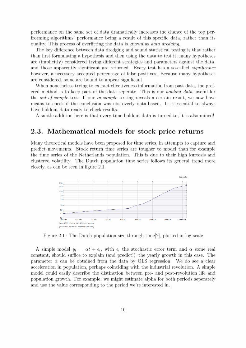
Many theoretical models have been proposed for time series, in attempts to capture andpredict movements. Stock return time series are tougher to model than for examplethe time series of the Netherlands population. This is due to their high kurtosis andclustered volatility. The Dutch population time series follows its general trend moreclosely, as can be seen in figure 2.1.

Figure 2.1.: The Dutch population size through time[2], plotted in log scale

A simple model yt = αt + εt, with εt the stochastic error term and α some realconstant, should suffice to explain (and predict!) the yearly growth in this case. Theparameter α can be obtained from the data by OLS regression. We do see a clearacceleration in population, perhaps coinciding with the industrial revolution. A simplemodel could easily describe the distinction between pre- and post-revolution life andpopulation growth. For example, we might estimate alpha for both periods seperatelyand use the value corresponding to the period we’re interested in.

10

Compare this graph to the historical value of the Dow Jones index shown in figure2.2. A more complex model is needed to generate data similar to the Dow values. Itshould come as no surprise that description, generation and prediction of such data ismuch harder, especially in the long term. A sizeable population of bankrupt traders canattest.

Figure 2.2.: Dow Jones Industrial Average values through time, plotted in log scale

In this section, such beefier models are considered, or merely dipped, into. Our aim forthis thesis is to compare model samples and historical data using our algorithm. Bothquantity (investment size) and quality (return) of trades matter here. The algorithmrelates to running maximum breaches, using the short-term mean reversion present ineconomic data to achieve a degree of predictability. Therefore my hypothesis is thatmodel trade quality will depend strongly on whether mean reversion is present in themodel.

One of the simplest models, no stranger in mathematicians’ circles, is called the Wienerprocess. The Wiener process is the model used to describe Brownian motion, it was notmade to fit financial data! Brownian motion was famously first observed by RobertBrown in 1827, looking at tiny particles bouncing through a microscope. We are inter-ested in the one-dimensional analogue.

A Wiener process in our case is a continuous-time, real-valued stochastic process W .It is characterized by the following properties[3]:

1. W0 = 0

2. The function t→ Wt is continuous in t with probability 1

3. The process has stationary, independent increments

4. The increment Wt+s −Ws is distributed N (0, t)

The Wiener process can be viewed as the limit of rescaled simple (discrete) randomwalks [3]. This allows us to generate samples with a finite time step. In discrete form,the model takes on the form

∆W = ∆Wt ' ε√

∆t,

11

where ε ∼ N (0, 1), and values of ∆Wt are independent for any two time intervals ∆t.As there are no parameters, this model will not get it right often. Its (abundant) useslie outside finance. It does serve as a basis for other models, which is why it is includedhere.

Adding two parameters, which can be fitted to better model diverse (financial) data,results in the generalized Wiener process [4] denoted GW . These parameters are themean change per unit time, the drift rate, and the variance per unit time, the variancerate. This gives the opportunity to include a trend a ∈ R into the model, as wellas adjustable volatility controlled by b ∈ R. In analogue to the Wiener process, it isdescribed algebraically by

∆GW = a∆t+ bε√

∆t,

where ε ∼ N (0, 1) independently for any two values of ∆t.The generalized Wiener process seems a reasonable candidate to model financial time

series, to some extent. One key aspect of stock returns is not present yet, however.Returns in the generalized Wiener are dependent of price level, where this is never thecase for stocks. Instead of a constant trend (and constant rise in expected value) wedesire constant expected returns. This is achieved by the geometric Brownian motionprocess GBB, an expansion of the generalized Wiener process. It is described by

∆GGB = aGGB∆t+ bGGBε√

∆t, or∆y

y= a∆t+ bε

√∆t.

The geometric Brownian motion is widely used to model stock price behaviour[4]. TheBlack-Scholes-Merton option pricing equation is based on this stock price model. How-ever, this model does properly not reflect the excessive volatiliy which is at times presentin financial data.

Another class of model entirely, coming much more from a time series than from astochastic process-angle, is the so-called autoregressive process, or AR(1)[5]. In modelswith an autoregressive component, new values are explained in part by a function of theprevious values. It is described for a stock y at time t∗ by

yt∗ = αyt∗−1 + εt∗ ,

where εt∗ = ε ∼ N (0, σ2) independently, with α ∈ R and σ2 > 0 parameters. A constantmay be included on the right side to model a trend, yielding yt = αyt−1 + β + εt forβ ∈ R. The parameter σ2 describes the volatility, and α prescribes how fast shocks dieout. Note that for α = 1 the shocks do not die out, and we end up with a Wienerprocess. Also note that this simple model does display mean reversion!

As with the Wiener process, the AR is a relatively simple process not really fit tomodel complex time series such as those generated in finance. It is included here forcomparison’s sake and ease of use. An extension, used to model stock returns is GARCH,for General autoregressive conditional heteroskedasticity [6]. The distinctive feat of thismodel is its clustered volatility, allowing us to model the changing volatility occuring infinancial time series. This is achieved by including the previously fixed variance of εt

12

into the model. Mathematically, it is stated for a stock y at time t∗, as

yt∗ = µ+ εt∗

εt∗ ∼ N (0, σ2t∗)

σ2t∗ = a0 + a1ε

2t∗−1 + a2σ

2t∗−1,

with parameters µ ∈ R representing the long-term equilibrium, and a0, a1, a2 ∈ R≥0.These three must be positive as the variance σ2

t cannot be negative for any value of t.Both the previous outcome and the previous parameter value are incorporated in a newvolatility parameter value. This generates a situation where extreme returns (high orlow) in the recent past are indicative of future extreme returns. The same holds true forsmall returns. This is what is meant by clustered volatility.

We use Mathematica to generate series of data from the models. Wherever parametersare involved, these need to be estimated based on our dataset. The generalized Wienerand geometric Brownian processes require only sample drift and variance rates. Sampledrift requires a linear fit on the data, and variance is also estimated in the usual way.For AR processes, linear regression can also be used to estimate the parameters of themodel[5].

However, parameter estimation can also be an involved process. Parameters in theGARCH model are not directly observed, such as the variance in the geometric Brownian.Neither can they be calculated directly using some closed form expression involvingthe data, as the AR process’ parameter φ can be by ordinary least squares. Instead,calculation relies on maximum likelihood.

Given data and a mathematical model with parameters, maximum likelihood seeksto maximize the likelihood function (probability) L(θ|It) of the data occuring, over theparameters. Here θ is a vector including all parameters of the model, and It is the setof information at time t. This optimization yields the parameters most likely to yieldthe data we have. The calculation is different for every model. For an introduction tothe GARCH case, see [6]. The likelihood in terms of the GARCH parameters, assumingnormal conditional returns up until time t, can be written

L(α0, α1, α2, µ|r1, r2, . . . , rt) =1√

2πσ2t

e− (rt−µ)

2

2σ2t1√

2πσ2t−1

e− (rt−1−µ)

2

2σ2t−1 . . .1√

2πσ21

e− (r1−µ)

2

2σ21 .

To make the optimization easier, it is customary to maximize the log of the likelihoodl(θ|It) instead. It may be written

l(α0, α1, α2, µ|r1, r2, . . . , rt) = − t2

log(2π)− 1

2

t∑i=1

log(σ2i )− 1

2

t∑i=1

(ri − µ)2

σ2i

.

We substitute σ2i = α0 + α1ε

2i + α2σ

2i−1 in the latter equation and proceed to take

derivatives to a parameter. We set the derivative equal to 0 to solve for an expressionfor that parameter. Note that the initial volatility value σ2

1 also needs to be estimated,though for time series containing a lot of data its exact value will not matter much. Theoptimizations are not always easy and linear. For this project, we rely on Mathematicato execute them.

13

3. Algorithm and performanceanalysis

The performance of the algorithm I constructed is evaluated. First, it is briefly intro-duced. For a more elaborate explanation on how it was conceived, see the internshipchapter in the appendix. In the second section we analyze performance on the historicalhigh frequency data sample. In the third section we compare this to performance ondata generated according to theoretical models.

3.1. My first algorithm

The algorithm spends most of its time monitoring current and recent past prices forevery stock, looking for what I’ve come to simply call events. It enters a position if andonly if it encounters an event in the data. Because of the specification of an event, bymy research stocks tend to react with a price fall following an event. This price fall iscapitalized on in the span of just around an hour and a half, depending on how fast thestock sells off when the position is closed.

We consider a point (k, i, j) in our time × date × stock-space to be an event for fixedparameters if

• The stock j is, at this time i, at its running daily maximum, e. g. price(k, i, j) >price(p, i, j) ∀p ∈ {0, . . . , k − 1}.

• The stock j has a return of at least 2% over the 30 minutes before time k.

• At time k, bid-ask spread of stock j is at most 0.1%, or 10 basis points.

Dropping the demand of fixed parameters, we may change the minimum rise demand,as well as the time in which this is to take place and the maximum spread at the currenttime. We may also change how long we enter our position after an event, the defaultfrom observation of reaction curves is set at 100 minutes. We expect the collection ofevents to remain largely constant under slight variation of the parameters due to overlap.This serves as a check against data dredging.

The demand of positive return guarantees us only stocks volatile on the short termare included. Without this demand, returns following an event were on average muchsmaller as very slow stocks happening to surpass their running daily maximum werealso included. The demand of low spread asserts that the market to be entered is inequilibrium, with the price not stemming from a sudden drop in supply or demand as

14

often happens early in the morning. This constraint is more practical of nature, as wecould not obtain the stocks at the mid price deemed so attractive if we tried, if thespread is too large.

3.2. Historical sample data performance

Using standard parameters and our (out-of-sample!) data set the algorithm yields thefollowing, promising, euro, profit-to-day graph over all data:

Figure 3.1.: Cumulative profit using the algorithm with default parameters

The largest single loss, clearly visible in the image above on the top right, takesplace on day 382 and indeed seems no more than an unlucky bet: Shorting resultedin a negative return of 10%, one of the most extreme in all of the dataset, over oneof the largest investments. This investment still shrivels in size compared to the totalinvestment, so the largest loss seems in check.

A rule of thumb for profit graphs states that the underlying algorithm is promisingonly if the steepest decline in the graph is less than half of the total height of the graph.Our graph satisfies this rule.

In our sample of around 509 minutes of trading each day, 387 days and 1126 stocks, wehave a total of 2.22 · 108 possible times for events to take place. In these, our algorithmfound 3513 matches. This amounts to a 0.0016% chance for a stock to partake an eventat any given time. Due to the large amounts of data available, enough events may stillbe found.

15

Our bookkeeping variables allow us to check for occurances of skewness in them. Wewant to make sure , one day, stock or time does not have have a controlling impacton the shape of the profit curve. In this case, odds of reproducibility would be lowas we probably data dredged and the algorithm would not work on a different dataset. We prefer a generally uniform distribution of profits and event occurence overthe bookkeeping variables. Events are distributed through the days, intraday time andstocks according to figures 3.2, 3.3 and 3.4, respectively.

Figure 3.2.: Number of events occuring per sample trading day

16

Figure 3.3.: Number of events occuring per sample trading time

Figure 3.4.: Number of events occuring per sample stock

Note that in figure 3.3 a skewness is present towards the morning. This can be

17

explained by the fact that in the morning it is much more likely for a stock to breachits running daily maximum, a prerequisite for an event. This suggests other measuresof short-term average exceeding combined with the other event prerequisites might alsoyield great results, while making more use of the later parts of trading days.

Distribution of events through days and stocks is not completely uniform either. Thisis to be expected, however. Financial markets are infamous for their sudden and extrememovements. Profit is bound not to be made at a constant rate, unless we further splitour investments. The levels of skewness seem acceptable.

We also have access to the distributions of our investments and returns. Both displayedbelow in figures 3.5 and 3.6, respectively. Their respective means are 3.10 · 104 and4.87 · 10−4.

Figure 3.5.: Histogram of all realized investments

The shape of the histogram in figure 3.5 is easily explained. For the majority of ourtrades, less than the set maximum of 100000 euros can be invested in the stock. Becausefor every euro invested in the stock another β euros have to be invested in the future,the total invested per trade may exceed 100000 euros. Some high-volatility stocks haveβ > 1.5 on some days, resulting in a total investment exceeding 250000 euros.

18

Figure 3.6.: Histogram of all realized log returnsx

The most striking aspect of the returns is their average. This should approximatelyequal the average return, total profit divided by total investment. Instead, it is only half.This might be explained by the correlation between small investments and relativelyextreme returns. Both occur in quiet markets: without much action going on, ask andbid volumes are small. This also means demand or supply might drop suddenly. Forexample, a single buy offer might make up most of the ask volume. This results indramatically changed buy or ask prices without the other budging much. The mid pricedoes notice this, and responds to it. This causes artificial volatility the algorithm picksup, resulting in small trades.

On a side note, the series of returns has a kurtosis of over 11. Contrary to what thehistogram might suggest, a normal distribution is an abysmal model for them.

The total investment amounts to 1.09 · 108. This is spread out over 387 days however,and even within those days not all trades occur simultaneously. As can be seen in figure3.7, displaying the total amount invested per sample day, the highest amount investedat any point is 1.50 · 106.

19

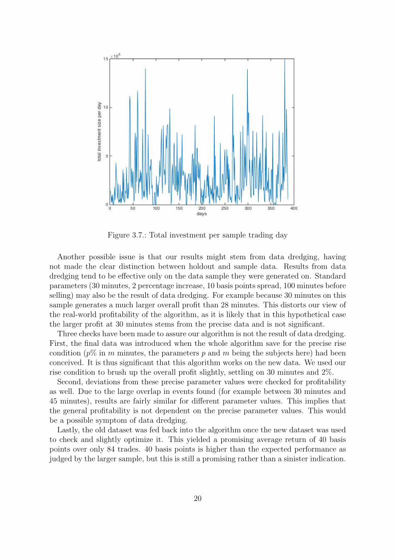
Figure 3.7.: Total investment per sample trading day

Another possible issue is that our results might stem from data dredging, havingnot made the clear distinction between holdout and sample data. Results from datadredging tend to be effective only on the data sample they were generated on. Standardparameters (30 minutes, 2 percentage increase, 10 basis points spread, 100 minutes beforeselling) may also be the result of data dredging. For example because 30 minutes on thissample generates a much larger overall profit than 28 minutes. This distorts our view ofthe real-world profitability of the algorithm, as it is likely that in this hypothetical casethe larger profit at 30 minutes stems from the precise data and is not significant.

Three checks have been made to assure our algorithm is not the result of data dredging.First, the final data was introduced when the whole algorithm save for the precise risecondition (p% in m minutes, the parameters p and m being the subjects here) had beenconceived. It is thus significant that this algorithm works on the new data. We used ourrise condition to brush up the overall profit slightly, settling on 30 minutes and 2%.

Second, deviations from these precise parameter values were checked for profitabilityas well. Due to the large overlap in events found (for example between 30 minutes and45 minutes), results are fairly similar for different parameter values. This implies thatthe general profitability is not dependent on the precise parameter values. This wouldbe a possible symptom of data dredging.

Lastly, the old dataset was fed back into the algorithm once the new dataset was usedto check and slightly optimize it. This yielded a promising average return of 40 basispoints over only 84 trades. 40 basis points is higher than the expected performance asjudged by the larger sample, but this is still a promising rather than a sinister indication.

20

3.3. Theoretical sample data performance

In order to best compare results between the historical and the theoretical data, themetrics used to compare performance with the theoretical data are also calculated forthe historical data. Event quantity is measured by the observed probability of an eventoccurring (mentioned last section, at 0.0016% for the historical data). The (average)response to an event, and specifically the average of all returns 100 minutes after everyevent, measure event quality. This last number will be different from our profit figurebecause trades are not weighed by the amount of shares available. It will also not equalour average return size, because it is calculated slightly differently. The historical datahas an average response of −7.5 basis points 100 minutes after the events. Overall andaverage response to an event are shown below.

Figure 3.8.: Reaction to an event for every event in the historical data

Figure 3.9.: Average reaction to an event in the historical data

21

In the generalized Wiener data sample, 2512 events occur in 509000 moments where anevent could take place, an observed event probability of 0.49%. The unweighed averagereturn over a long position taken after each event is −0.27 basis points.

Figure 3.10.: Reaction to an event for every event in the generalized Wiener data

Figure 3.11.: Average reaction to an event in the generalized Wiener daa

In the geometric Brownian data sample, 1749 events occur, again out of 509000 thatcould have. This amounts to an observed event probability of 0.34%. The unweighedaverage return over a long position taken after each event is 2.3 basis points.

22

Figure 3.12.: Reaction to an event for every event in the geometric Brownian data

Figure 3.13.: Average reaction to an event in the geometric Brownian data

In the GARCH(1,1) data sample, 2615 events occur out of again 509000 possible eventoccurances, an observed event probability of 0.51%. The unweighed average return overa long position taken after each event is 1.16 basis points

23

Figure 3.14.: Reaction to an event for every event in the GARCH(1,1) data

Figure 3.15.: Average reaction to an event in the GARCH(1,1) data

For data generated by all three models, the algorithm clearly does not work well.Events occur much more frequently in all theoretical data (by a factor of magnitude103, conservatively estimated), but no clear-cut response follows an event in any of thetheoretical models. This once again proves computers do not completely define intradaystock prices yet: clear marks of human sentiment can be found in the historical data,exploited by the algorithm but not present in the models taught to our students ofeconometrics. Because of the large size of the data set, it is unlikely that this basicresponse is explained by chance alone.

24

4. Conclusion

By not being able to disprove it using the checks in the previous chapter, we haveasserted that it is possible to make a profitable trading strategy centered around stocksexceeding their running daily maximum. Though averagely a mean reversing trend isvisible in historical stock price data following a running daily maximum pass, this trendis too weak to actively generate a profit trading. Essential additional requirements beforeentering a trade were found to be a steep price increase preceding the maximum breach,and a limit to the spread at the time of purchasing.

Other additions were also considered but did not improve the performane of the algo-rithm on our test samples. These include demanding at least n times the maximum isexceeded in m minutes, demanding there be a new running minimum in the m minutespreceding the running daily maximum breach, applying the algorithm to running min-ima, changing the maximum demand to be only the maximum of the past 3 hours, or amore ‘continuous’ version of the maximum, taking the position a few minutes after themaximum, and cutting our losses by selling as soon as a certain loss is reached.

The algorithm saw many more opportunities to enter positions in data generated ac-cording to theoretical models, but the profit from all those trades seems completelyunpredictable. The algorithm does not reliably generate any profits, or losses indicatingthat ‘shorting the algorithm’, setting up the opposite position following an event, mightyield positive results. The structure of how the market tends to react to running maxi-mum breaches is thus not included in the models, eventhough mean reversion sometimesis in other forms.

Looking back, the main point of improvement in this project would be stricter surveil-lance of what constitutes in sample data, and consequently what exactly the holdoutdata was and when it was to be used. Though no evidence nullifying the conclusionsof this research was found during the research itself, guarding the holdout data morecarefully would have improved the significance of the conclusions.

From this point, the best way to estimate the quality of the algorithm is to programit into a real time paper trading simulator. This would be my next step in research, ifI had more time on my hands. A larger, fresh data set would also shed further light onits profitability. Additional variations of the algorithm could also be devised.

25

5. Popular summary

As possibly the epitome of human progress, we have endowed computers with the abilityto trade stocks for us. Computers do not get tired, never demand a pay raise, keep muchmore detailed track of many more stocks and, importantly, never let emotions get in theirway. But, given the opportunity, by which measure would you have your digital traderarmy trade?

For this thesis I was given an internship at Deep Blue Capital and the opportunityto specify one such algorithm. No actual positions were entered by my algorithm, butthe algorithm was implemented in Matlab and used on a historical data set consistingof prices of over 1100 stocks, over the period August 2014 - February 2016. This helpedformulating and testing it, but obviously offers no guarantees.

In order to let our computers trade, we need to specify what sort of positions itshould enter in certain situations. The computer then scans stock price developmentsaround the world (or whatever part we desire) looking for said situations. My internshipcounselor Robin de Vilder gave me a broad class of situations after which a certaindegree of predictability might be present. These situations are the times at which astock attains the highest value it had so far during the day. We call this highest valueso far the running daily maximum. In such ‘extreme’ situations, a phenomenon calledmean reversion tends to come into play. It tells us here that stocks at their runningdaily maximum tend to revert to their short-term average price, dropping in price in theprocess.

To assure that stocks are indeed out of equilibrium, we also demand that in the timeprior to a stock attaining its running daily maximum, it rises relatively sharply. Beforeentering a position we also check that the highest price the stock is bought for and thelowest price the stock is sold at, the so-called bid and ask prices, do not differ overlymuch. this might indicate market turmoil or prices which are overly volatile due to lowbid and ask volumes, bad times to buy. Using these rules, the algorithm entered around3500 hypothetical positions in the sample data. The cumulative profit of these tradesover the time period August 2014 - February 2016 is shown in the following figure.

26

Figure 5.1.: Cumulative profit using the algorithm with default parameters

Mathematical models have been developed in order to analyze and predict the move-ment of stock prices. Data was generated using these models, and the algorithm wasapplied to that data. The algorithm did not yield favorable results with any of the mod-els’ data, even though a certain degree of mean reversion is present in some of the models.The inherent predictability present in the current markets, used by my algorithm, couldbe concluded to be due to human effects, even while computers dwarf humans in tradevolume.

27

Bibliography

[1] Wired.com, checked 1 april 2016. http://www.wired.com

[2] Wolframalpha.com, checked 1 may 2016.http://www.wolframalpha.com/input/?i=dutch+population+size+through+time

[3] S Lalley, Lecture 5: Brownian Motion, Mathematical Finance 345, 2001.http://www.stat.uchicago.edu/ lalley/Courses/390/Lecture5.pdf

[4] J C Hull, Options, futures and other derivatives - 8th ed, p284-286, Pearson, 2012.

[5] C Heij et al, Econometric methods with applications in business and economics, p558-560, Oxford, 2004

[6] R Reider, Volatility forecasting I: GARCH Models, Time Series Analysis and Statis-tical Arbitrage, 2009. http://cims.nyu.edu/ almgren/timeseries/Vol Forecast1.pdf

28

A. Internship

This chapter contains a week-to-week description of my activities at Deep Blue Capital.I recommend those not active in financial mathematics to scan chapter 2 first. Much ofthe parlance introduced is used here.

Week 1

I started at Deep Blue on February 18th, 2016. After brief introduction to the firm andits employees, I set to work. At my disposal was a data set consisting of several attributes(Bid, ask, and mid prices, as well as ask- and bid-volumes) of a number of Europeanstocks. The corresponding index used to calculate β’s cannot be traded directly (nonecan). We obtain prices corresponding to the index returns from a future representingthe index, also included in the data. Furthermore, the data contained a set of dailyvalues for more attributes for all stocks (opening price, closing price, etcetera) also usedto calculate β.

I started off working towards β-corrected log returns of all stocks, per 5 minutes,using a β calculated seperately for each day and stock. Because the stocks are basedin several different countries, the data was rather non-homogeneous, however. All dayshave measurement points ranging from 8:00 till 18:00, but different stocks start, interruptand stop trading at different times. The array of prices displays a NaN in the case ofsuch an interruption. Making the dataset homogeneous proved the first challenge.

This being the first week I naively tried to hardcode this myself. Mistakes were made,including but not limited to the following. I took the last price of the day for the futureinstead of the price corresponding to the moment the stock stops trading for the day. Itried to catch all the different trading times for different stocks manually. I hardcodedall sorts of numbers that turned out to be variable, such as the number of data pointsper day. The gauging of the β’s also took some work.

Help from Victor resulted in better Matlab code. This generates a 3d array containinga datapoint for each day for each moment for each stock. A serpate array was madecontaining a datapoint for each day for each moment for the future. These arrays stillcontained NaNs. From this we could calculate all β values.

One of β’s properties may be used to check empirically if the retrieved values arecorrect. For a day i, βi minimizes Var(rs−βrf ), taking again the last 59 observations ofboth series. So for x ∈ [0, 2] we may plot Var(rs−xrf ) and see if the minimum is indeedattained at the value of βi This turned out to be the case for several randomly chosendays. A comparison with β’s supplied by Bloomberg did not show large deviationseither. These checks assure results so far were correct.

29

Week 2

Victor gave me a larger data set, with data points for each minute for each stock, takenover more days. The procedure so far was applied to this set, too. Armed with thecorrect β’s, I could calculate market neutral minute-to-minute log returns. Taking thecumulative sum of these returns yielded the standardized and market neutral stock pricedevelopment. Several hickups occurred finalizing this, but a Thursday afternoon provedalmost enough to iron out the details. Many exceptions had to be taken care of, such asthe NaNs still present in the array of corrected series and a stock without valid entriesfor the first 100 days. I noted that some β’s were negative, from which no apparentproblems arose.

From the cumulative market neutral log returns of the stocks, we could now set upa boolean-filled matrix of the same size containing for every moment for every day forevery stock whether or not the stock passes its running daily maximum at that moment.This matrix is the basis of our investigation. We could repeat the proces for both minimaand total extrema, as well as other attributes. But focus was on the maxima.

This opened up many opportunities and questions to research. It may be no largesurprise that the first question I asked myself, in retrospect, is not a very informativeone. I decided to compare the total amount of extrema breaches in a day, to suitableAR(1) and generalized Wiener models. For the Wiener model, I found that the variancerate in the normal does not influence the amount of extrema breaches.

In the AR(1)-model yt = αyt−1+εt, fitting α, which can be done via a simple regressionof yt on yt−1, resulted for every day and every stock in an α greater than 0.99. Greater αresulted in fewer extrema breaches, however taking α > 1 will not result in a stationaryprocess and our data had fewer breaches still, so the model seemed unfit to modelextrema breaches in financial time series.

In the generalized Wiener model, adding a trend to the normal increased the amountof extrema breaches. However, even with no trend, the amount of extrema was muchlarger than that in the data.

Week 3

Figures were made of the running day maxima, for both simulated model and the data.This was done using a single self-written function that simply takes a time series, com-putes the running maxima and plots them. Because the AR-parameters depend on thestock chosen, the stock highest in my data folder, with number 101, was picked to al-low for comparison. A resulting average plot was generated too, for both model andsimulations. A selection is shown below.

30

Figure A.1.: A plot of daily cumulative market neutral log returns for stock 101 for everyday

Figure A.2.: A plot of around 400 simulations, generated using brownian motion

Figure A.3.: A plot of the running maxima of the previously shown BM-generated series

31

Figure A.4.: A plot of the average of the running maxima of the stock

Note that figure A.4 does not just display the square root-like shape we might expect.Instead, there seem extra maximum breaches in the late afternoon. Models additionallyrequired to display this behaviour may need an additional component reflecting afternoonmarket behaviour.

Another question we may ask, using last week’s boolean matrix, is what a stock tendsto do after it reaches a maximum. To visualize this, we plot the average of the cumulativereturns for a certain amount of minutes after a maximum breach, for every maximumbreach in our data set. Doing this for several consecutive minutes, we deduce an ‘averageresponse’, to a maximum breach for all stocks. The result seems surprisingly continuous.

Figure A.5.: A plot of the average reaction to a maximum breach, against the amountof minutes since the breach

This also holds for the event of a minimum breach, though with a smaller rebound:

32

Figure A.6.: A plot of the average reaction to a minimum breach, against the amount ofminutes since the breach

As a followup topic, on Thursday a start was made towards generating such plots formore complex, compound events such as (at least) n maximum breaches in the last mminutes. Several results were gathered for small values of m and n.

Week 4

More time was spent debugging the previously mentioned script. Sadly, once runningthe program showed there is little money to be made using the strategy it implemented,regardless of the combination of m and n. Because so many combinations exist, outliersare bound to be present so a single combination yielding a positive result was not enoughto compensate for the general lack of structure and probably the result of data dredging.

First steps were made towards a more promising idea: demanding a certain price risein addition to attainment of a daily maximum (extremum) before a moment is to bemarked as an event. For example, we might demand that a stock attain its running dailymaximum and was at least 2% lower an hour earlier. This idea quickly became the mainfocus for my trading algorithm, though other algorithms using maximum breakthroughswere considered in weeks 5.

Week 5

Another take at the problem is attempted, marking a (time, day, stock)-pair as an eventonly if the stock is now at an extremum and attained its opposite extremum within acertain amount of minutes ago. For an example, we might set an event to be any stockexceeding its running minimum while having exceeded its running maximum within thelast hour. Again, sadly, no fortunes flow from this strategy, as no clear average behaviourfollows the event.

To find out what might explain seemingly significant results from the algorithmslooking at past events, I made it possible to plot the series from the event till 90 minutes

33

after the event for every event, rather than just the average. This way, an outlierinfluencing the average at a certain time after the event may easily be spotted.

Strongly correlated events were filtered from the results by letting the algorithm skipto the next day immediately after an event has been found. For example, demanding8 rises of the running maximum in the last 10 minutes will find 4 seperate events in astock exceeding its maximum 12 times in a row! This way, extra significance is put onthe movement of the stock after roughly the first time the event took place, as the otherevents strongly correlate with it. This might cause seemingly significant effects in theaverage response, making it a very unwanted effect. In order to remove it, a stock is notconsidered for 40 minutes after an event took place.

To keep track of the distribution of the events over days, stocks and time of days,different lists are created keeping track where each event lies in each of these threedimensions. A histogram shows the vast majority of running maximum breakthroughsoccurs in the first twenty percent of a day. Because spreads are much higher during theopening hour, roughly, a check for low bid-ask spread is added to the event demands.

Events occuring in the last hour of trading also turned out to skew our results, andwere excluded. In these cases, the exchange would close before we could close ourposition. To still have some price for the stock, we kept the price of the now-untradablestock at the price it had right before trading stopped. This might lead to impossibletrade orders, hence the exclusion.

An attempt was made to pour all working code into a single Matlab function requiringonly the data set, so the algorithm could be tested other sets. No other data was availableyet, however.

Week 6

I could only work on my internship for a single afternoon due to Good Friday and some ofmy final exams. The events where a running extremum breakthrough was foreshadowedby its opposing running maximum breakthrough also turned out not to harbour a greatdeal of trading opportunities. A data set was offered by Victor to test the functionmentioned above, but it didn’t suffice as it only contained 14:00-15:30 of every tradingday. Part of this chapter was written, to prevent order and details from being forgotten.

Week 7

This week marked the start of April, during which I worked at Deep Blue almost full timerather than a day and a half a week, as had previously been the case. Simultaneously,the general idea of this thesis crystallized.

I was given a larger dataset by Victor, containing minute-to-minute data of 1126stocks over the course of 387 days. The prepared function to analyze the data at onceturned out not to work. It could not handle the data size increase efficiently. However,it contained a lot of analysis which was not required in the algorithm eventually judgedmost promising. Removing this resulted in a script that translates the 27GB in data

34

to workable matrices in around 20 minutes. This script only needs to be run once afterevery Matlab restart. Versions of the trading algorithm all run in under 20 seconds.

Because companies fail, merge or change structure, a reasonable amount of incom-pleteness was expected in the data. This turned out to be the case, with 220 stocksmissing β values for more than 20 days. The solution is simple however, using all stock-day pairs for which a β can be found rather than excluding irregular stocks. This yieldsus the most valid days, excluding all invalid ones.

By changing the algorithm to not look 90 seperate minutes after an event but only the90th one, I was able to squeeze all data into a single matrix. This allowed the algorithmto work all data at once rather than a sixteenth per run.

Because mid prices behave curiously when bid-ask spreads become large, we decideto add a requirement of ”small spread” on all our potential events. This yields the finalspecification of an event, as discussed in the Results chapter.

Week 8

Due time for a test run of the algorithm. I decided to close the historical deals intwo ways, to double check. Via the cumulative returns array of all stocks, and directlyby buying and selling at the then current prices. This filtered several sign bugs, butdebugging well into week 8 revealed that in cases where a price is left undefined inbetweenevent and closing time the first method skips an inbetween return. This leaves usprefering the second method of setting up the historical deal. It is displayed in Matlabcode appendix A.

At this point, save for some extentions, work on the algorithm was done. I decided toapply the algorithm to data sampled from theoretical models to compare performance.The algorithm in its final shape based on minima breaches was created, but workedmuch worse than the maximum-based version.

A quick test was performed by applying the final algorithm with standard parametersto the previous, smaller minute-to-minute data set. The average sample return per tradeamounted to 36 basis points over 84 events in the data. This is better than I expect thealgorithm to perform on average, but a positive indication.

Week 9

Both Asma and Robin were met with, and their initial feedback on the thesis wasincorporated. Because in its current setup the algorithm trades mainly in the morning,two attempts were made to replace the ‘running daily maximum exceeding’ demand foran event by a more continuous version. First, the running maximum was required onlyto be of the past 3 hours. This yielded a weaker average response, evaporating possibleprofits.

The second idea is perhaps best explained by figure A.7. We replace the runningmaximum by a ‘falling maximum’, dropping by 0.1% every minute. This way, moreevents take place later in the day.

35

Figure A.7.: a stock’s daily falling maximum

Compared to the standard version of the algorithm these changes only add about 100events and no notable profit, discouraging their addition.

Instead of entering a position right at the maximum, a version I implemented waited5 more minutes to see if another maximum took place. This attempt to weed out thecases where the stock goes up instead of down did not work out.

Another version concerned itself with just the stock returns, rather than their marketneutral transforms. It performed significantly less well on the sample data, indicatingmarket neutral is the way to go.

Victor also generated the results of applying the algorithm to the data set. By back-tracing individual events several explanations for the differences between our resultswere found. I looked back 29 rather than 30 minutes and sold after 100 rather than 90minutes, for example. We also used slightly different β values. The algorithm survivedthe test.

Week 10

Versions of the algorithm were created that close the position at either a certain profitor loss. The first case prevents a possibly worse loss, the second case cashes in beforethe profit potentially evaporates. This led to returns such as those displayed in A.8.

36

Figure A.8.: Returns when positions are closed whenever 2% loss is reached

All of these versions had lower return and profit than the original algorithm. Strivingto keep the algorithm as minimal as possible to avoid data dredging, I decided not toadd the changes to the algorithm.

Furthermore, sample data of the three discussed theoretical models was generated.Adapted versions of the algorithm were written to analyze the generated sample data.

37

B. Matlab code

Data and structure setup

The following script was run to gather the data from a folder of tables of past values.Data is gathered into matrices which allow for a relatively high-level description of thealgorithm.

import_list = dir(’/Users/Nout/Documents/Stage’);

% Importing all symbols by name from the folder

symbols = [];

for d = 1 : length(import_list)

name = import_list(d).name;

if length(strfind(name, ’day’)) > 0

pos = strfind(name, ’-’);

symbols = [symbols, str2num(name(1 : pos - 1))];

end

end

clearvars import_list name pos;

% Remove the futures (id’s 29 and 45) from the symbols list

symbols(find(symbols == 29)) = [];

symbols(find(symbols == 45)) = [];

% Import intraday future data to classify days and times

fu_sym = 45;

fu1m = importdata(strcat(int2str(fu_sym), ’-data_1min.dat’));

fu1m = fu1m.data;

dates = unique(floor(fu1m(:, 1)));

nr_t = length(find(floor(fu1m(:, 1)) == dates(1)));

nr_d = length(dates);

nr_s = length(symbols);

38

% Generate a matrix for each required interday attribute. 15 at most.

T_closes = zeros(nr_d, nr_s) * NaN;

price_closes = zeros(nr_d, nr_s) * NaN;

for j = 1 : nr_s

st_day = importdata(strcat(int2str(symbols(j)), ’-data_day.dat’));

if isfield(st_day,’data’)

st_day = st_day.data;

[l, b] = size(st_day);

if l == nr_d && b == 15

T_closes(:, j) = st_day(:, 4);

price_closes(:, j) = st_day(:, 5);

end

end

end

% Generating future close prices. Checking an interval to evade NaNs

fu_closes = zeros(nr_d, nr_s) * NaN;

indices2 = find(fu1m(:, 2) > 0);

for i = 1 : nr_d

for j = 1 : nr_s

indices = find(abs(T_closes(i, j) - fu1m(:, 1)) < 2 / (24 * 60));

indices = intersect(indices, indices2);

if ~isempty(indices)

X = [fu1m(indices, 2), abs(T_closes(i, j) - fu1m(indices, 1))];

X = sortrows(X, 2);

fu_closes(i, j) = X(1, 1);

end

end

end

clearvars indices indices2 X st_day

39

% Generating stock prices and quantities for each day and moment

sts_mids = zeros(nr_t, nr_d, nr_s) * NaN;

sts_bids = zeros(nr_t, nr_d, nr_s) * NaN;

sts_asks = zeros(nr_t, nr_d, nr_s) * NaN;

sts_bid_vs = zeros(nr_t, nr_d, nr_s) * NaN;

sts_ask_vs = zeros(nr_t, nr_d, nr_s) * NaN;

for j = 1:nr_s

st1m = importdata(strcat(int2str(symbols(j)), ’-data_1min.dat’));

if isfield(st1m, ’data’)

st1m = st1m.data;

[l, b] = size(st1m);

if l == nr_t * nr_d && b == 6

for i = 1 : nr_d

sts_mids(:, i, j) = st1m((i - 1) * nr_t + 1 : i * nr_t, 2);

sts_bids(:, i, j) = st1m((i - 1) * nr_t + 1 : i * nr_t, 3);

sts_asks(:, i, j) = st1m((i - 1) * nr_t + 1 : i * nr_t, 4);

sts_bid_vs(:, i, j) = st1m((i - 1) * nr_t + 1 : i * nr_t, 5);

sts_ask_vs(:, i, j) = st1m((i - 1) * nr_t + 1 : i * nr_t, 6);

end

end

end

end

% Generating future prices and quantities for each day and moment

fu_mids = zeros(nr_t, nr_d) * NaN;

fu_bids = zeros(nr_t, nr_d) * NaN;

fu_asks = zeros(nr_t, nr_d) * NaN;

fu_bid_vs = zeros(nr_t, nr_d) * NaN;

fu_ask_vs = zeros(nr_t, nr_d) * NaN;

for i = 1 : nr_d

fu_mids(:,i) = fu1m((i - 1) * nr_t + 1 : i * nr_t, 2);

fu_bids(:,i) = fu1m((i - 1) * nr_t + 1 : i * nr_t, 3);

fu_asks(:,i) = fu1m((i - 1) * nr_t + 1 : i * nr_t, 4);

fu_bid_vs(:,i) = fu1m((i - 1) * nr_t + 1 : i * nr_t, 5);

fu_ask_vs(:,i) = fu1m((i - 1) * nr_t + 1 : i * nr_t, 6);

end

clearvars st1m

40

% Generating interday log returns to calculate betas.

logreturnssts = zeros(nr_d - 1, nr_s);

logreturnsfu = zeros(nr_d - 1, nr_s);

for i = 1 : nr_d - 1

logreturnssts(i, :) = log(price_closes(i + 1, :) ./ price_closes(i, :));

logreturnsfu(i, :) = log(fu_closes(i + 1, :) ./ fu_closes(i, :));

end

% Generating betas. We require 45 valid days, that is no NaNs in the log

% returns, in the last 60 days. beta is NaN if this is not the case.

betas = zeros(nr_d, nr_s);

for i = 61 : nr_d

for j = 1 : nr_s

st_3mnth = logreturnssts(i - 60 : i - 2, j);

fu_3mnth = logreturnsfu(i - 60 : i - 2, j);

nans_st = isnan(st_3mnth);

nans_fu = isnan(fu_3mnth);

nans = nans_st + nans_fu;

st_3mnth(find(nans)) = [];

fu_3mnth(find(nans)) = [];

if length(st_3mnth) > 45

temp_cov = cov(st_3mnth, fu_3mnth);

betas(i,j) = temp_cov(2,1)/temp_cov(2,2);

else

betas(i,j) = NaN;

end

end

end

for i = 1 : 60

betas(i, :) = betas(61, :);

end

clearvars nans nans_fu nans_st st_3mnth fu_3mnth temp_cov

41

% Generating intraday log returns and spreads.

intraday_logreturnsst = zeros(nr_t - 1, nr_d, nr_s);

intraday_logreturnsfu = zeros(nr_t - 1, nr_d);

intraday_spreadsst = log(sts_asks ./ sts_bids);

for k = 1 : nr_t - 1

intraday_logreturnsst(k, :, :) = log(sts_mids(k + 1, :, :) ./ sts_mids(k, :, :));

intraday_logreturnsfu(k, :) = log(fu_mids(k + 1, :) ./ fu_mids(k, :));

end

% Generating market neutral series using intraday log returns. NaNs are

% converted to zeros here, so the cumulative sums aren’t messed up.

marneut = zeros(nr_t - 1, nr_d, nr_s);

for i = 1 : nr_d

for j = 1 : nr_s

marneut(:, i, j) = intraday_logreturnsst(:, i, j)

- betas(i, j) * intraday_logreturnsfu(:, i);

for k = 1 : nr_t - 1

if isnan(marneut(k,i,j))

marneut(k, i, j) = 0;

end

end

end

end

% Generating cumulative market neutral series, to locate maximum breaches.

marneut_csum = zeros(nr_t - 1, nr_d, nr_s);

for i = 1 : nr_d

for j = 1 : nr_s

marneut_csum(:,i,j) = cumsum(marneut(:,i,j));

end

end

42

% Generating running daily maxima.

maximum_bool = zeros(nr_t - 1, nr_d, nr_s);

for i = 1 : nr_d

for j = 1 : nr_s

dagmax = 0;

for k = 2 : nr_t - 1

price = marneut_csum(k, i, j);

if price > dagmax

maximum_bool(k, i, j) = 1;

dagmax = price;

end

end

end

end

clearvars price dagmin dagmax b d i j k l fu1m

43

Trading algorithm

The algorithm below uses the output of the previous script, checking for events andresponding appropriately.

% Event = at least min_change in last mins_before and at most max_spread in

% current bid-ask spread. At an occerance we short st - beta * fu for

% mins_later minutes.

mins_before = 30;

min_change = 0.02;

max_spread = 0.001;

mins_after = 100;

% ---- setting bookkeeping variables -----

investments = [];

logret_invests = [];

total_investment = 0;

total_profit = 0;

profit_per_day = zeros(nr_d, 1);

picked_per_day = zeros(nr_d, 1);

picked_per_time = zeros(nr_t - 1, 1);

picked_per_stock = zeros(nr_s, 1);

44

% Browse all time x day x stock scouting events.

for i = 1 : nr_d

for j = 1 : nr_s

k = 1;

while k < nr_t - 120

if maximum_bool(k, i, j) == 1

t_passed = min(k - 1, mins_before - 1);

change_last_minutes = marneut_csum(k, i, j)

- marneut_csum(k - t_passed, i, j);

% Check for event

if change_last_minutes > min_change

&& intraday_spreadsst(k + 1, i, j) < max_spread

%-------- SETTING UP THE DEAL --------

% Look mins_after minutes after the transgression. Buy

% the available amount of stucks, limited at 100k euro.

nr_available = min(sts_bid_vs(k + 1, i, j),

floor(100000 / sts_bids(k + 1, i, j)));

% Short log return stock

sell_price_st = sts_bids(k + 1, i, j);

buy_price_st = sts_mids(k + mins_after + 1, i, j);

logret_invest_st = log(sell_price_st/buy_price_st);

% Long log return future

sell_price_fu = fu_asks(k + mins_after + 1, i);

buy_price_fu = fu_mids(k + 1, i);

logret_invest_fu = log(sell_price_fu/buy_price_fu);

% Weighed total log return

logret_invest = logret_invest_st

+ betas(i, j) * logret_invest_fu;

invest_size = nr_available * sell_price_st * (1 + abs(betas(i, j)));

invest_profit = invest_size * logret_invest;

45

%----- MAKING THE DEAL IF NO NANS OCCUR -----

if ~isnan(logret_invest)

% Updating bookkeeping variables:

picked_per_time(k) = picked_per_time(k) + 1;

picked_per_stock(j) = picked_per_stock(j) + 1;

picked_per_day(i) = picked_per_day(i) + 1;

investments = [investments; invest_size];

logret_invests = [logret_invests; logret_invest];

total_investment = total_investment + invest_size;

total_profit = total_profit + invest_profit;

profit_per_day(i) = profit_per_day(i) + invest_profit;

end

k = k + max(40, mins_before);

end

end

k = k + 1;

end

end

% Print i to check progress

i

end

% Quick summary

matches_in_data = length(logret_invests)

realistic_profits = total_profit/total_investment*10^4

% Generate profit graph

plot(cumsum(profit_per_day))

clearvars mins_before min_change max_spread mins_after change_last_minutes ...

t_passed nr_available sell_price_fu sell_price_st buy_price_fu buy_price_st ...

logret_invest_st logret_invest_fu logret_invest invest_size invest_profit ...

k i j

46