pebble - european commission : cordis · pebble, fp7-ict-2009-6.3, #248537, deliverable d2.3 i...
TRANSCRIPT
PEBBLE Positive-Energy Buildings through Better controL
dEcisions 248537, FP7-ICT-2009-6.3
Deliverable D2.3:
Simulation Model Improvements
Deliverable Version: D2.3, v.1.4
Document Identifier: pebble_wp2_deliverable_2-3_v1.4
Preparation Date: November 7, 2011
Document Status: Final
Author(s): M. F. Pichler, A. Dröscher, H. Schranzhofer, Ana Contantin, Max Huber, G. Giannakis, N. Exizidou, and D.V. Rovas
Dissemination Level: PP - Restricted to other programme participants (including the Commission Services)
Project funded by the European Community in the 7th Framework Programme
ICT for Sustainable Growth
Deliverable D2.3 Simulation Model Improvements
v. 1.4, 7/11/2011
Final
PEBBLE, FP7-ICT-2009-6.3, #248537, Deliverable D2.3 i
Deliverable Summary Sheet
Deliverable Details Type of Document: Deliverable
Document Reference #: D2.3
Title: Simulation Model Improvements
Version Number: 1.4
Preparation Date: November 7, 2011
Delivery Date: January 9, 2012
Author(s): M. F. Pichler, A. Dröscher, H. Schranzhofer, Ana Contantin, Max Huber, G. Giannakis, N. Exizidou, and D.V. Rovas
Document Identifier: pebble_wp2_deliverable_2-3_v1.4
Document Status: Final
Dissemination Level: PP - Restricted to other programme participants (including the Commission Services)
Project Details Project Acronym: PEBBLE
Project Title: Positive-Energy Buildings through Better controL dEcisions
Project Number: 248537
Call Identifier: FP7-ICT-2009-6.3
Call Theme: ICT for Energy Efficiency
Project Coordinator: Technical University of Crete (TUC)
Participating Partners:
Technical University of Crete (Coordinator, GR); Fraunhofer-Gesellschaft zur Förderung der Angewandten Forschung e.V.(DE); Rheinisch-Westfälische Technische Hochschule Aachen (DE); Technische Universität Graz (AU); Association pour la Recherche et le Developpement des Methodes et Processus Industriels - ARMINES (FR); CSEM Centre Suisse d’Electronique et de Microtechnique SA - Recherche et Dévelopement (CH); SAIA-Burgess Controls AG (CH)
Instrument: STREP
Contract Start Date: January 1, 2010
Duration: 36 Months
Deliverable D2.3 Simulation Model Improvements
v. 1.4, 7/11/2011
Final
PEBBLE, FP7-ICT-2009-6.3, #248537, Deliverable D2.3 ii
Deliverable D2.3: Short Description Work undertaken on WP2, on developing thermal simulation models is presented. The work moves in two directions: the first is the improvement of model accuracy by suitable calculations and the second is the development and evaluation of model-reduction techniques, for the creation of computationally-efficient thermal simulation models, with “just enough” accuracy, to be utilized in conjunction with the building optimization and control algorithms developed in D3.1.
Keywords: Thermal simulation model, Building modeling, validation, model-order reduction, CAO.
Deliverable D2.3: Revision History Version: Date: Status: Comments
1.0 19/12/2011 Draft HS: First version including all three parts
1.1 20/12/2011 Draft DVR: Edited the document for clarity, included new version for TUC building.
1.2 28/12/2011 Draft DVR, HS: Included text modifications
1.3 2/1/2012 Draft GG, DVR: Included TUC time constant
1.4 5/1/2012 Se
Copyright notice © 2012 PEBBLE Consortium Partners. All rights reserved. PEBBLE is an FP7 Project supported by the European Commission under contract #248537. For more information on the project, its partners, and contributors please see http://www.pebble-fp7.eu. You are permitted to copy and distribute verbatim copies of this document, containing this copyright notice, but modifying this document is not allowed. All contents are reserved by default and may not be disclosed to third parties without the written consent of the PEBBLE partners, except as mandated by the European Commission contract, for reviewing and dissemination purposes. All trademarks and other rights on third party products mentioned in this document are acknowledged and owned by the respective holders. The information contained in this document represents the views of PEBBLE members as of the date they are published. The PEBBLE consortium does not guarantee that any information contained herein is error-free, or up to date, nor makes warranties, express, implied, or statutory, by publishing this document.
Deliverable D2.3 Simulation Model Improvements
v. 1.4, 7/11/2011
Final
PEBBLE, FP7-ICT-2009-6.3, #248537, Deliverable D2.3 iii
Table of Contents Table of Contents ......................................................................................................................... iii List of Figures .............................................................................................................................. vi List of Tables .............................................................................................................................. viii Abbreviations and Acronyms ....................................................................................................... ix
A Introduction ......................................................................................................................... 1 A.1. Introduction ........................................................................................................................... 2
B FIBP Building Simulation .................................................................................................. 4 B.1. Introduction ........................................................................................................................... 5 B.2. Changes and improvements of the model ............................................................................. 5
B.2.1 Constructive changes made to the building model ....................................................... 5 B.2.1.1 Thermally Activated Building Systems (TABS) ................................................................ 5 B.2.1.2 Window size and shape .................................................................................................... 5 B.2.1.3 Duct system for the mechanical ventilation ..................................................................... 5
B.2.2 General parameter changes ........................................................................................... 6 B.2.3 Improvement and Refinements ..................................................................................... 6
B.2.3.1 Natural Ventilation via window opening dependent on CO2 concentration ..................... 6 B.2.3.2 Estimation of illumination................................................................................................ 6
B.3. Predictive data & data assimilation with the real building ................................................... 7 B.3.1 Predictive data and their modeling ............................................................................... 7
B.3.1.1 Occupancy and user behavior ......................................................................................... 7 B.3.1.2 Weather data .................................................................................................................... 8
B.3.2 Model assimilation ........................................................................................................ 8 B.3.2.1 Initial Conditions and settling phase ............................................................................... 8 B.3.2.2 Initial conditions and model settling for TRNSYS ............................................................ 9
B.3.3 The building time constant ........................................................................................... 9 B.3.3.1 Measuring of the building time constant ........................................................................ 10 B.3.3.2 General simulation parameters ..................................................................................... 10 B.3.3.3 Conditions and analysis for free floating and empty building ....................................... 10 B.3.3.4 General empirical model to fit data ............................................................................... 11 B.3.3.5 Further simulation results for the building time constant and interpretation ................ 12
B.4. Model complexity and calculation time .............................................................................. 12 B.4.1 Embedded MATLAB (Type155) in TRNSYS ............................................................ 12
B.4.1.1 Shared functionality and controllers in the building model ........................................... 12 B.4.1.2 Characteristic zones and interface with MATLAB ......................................................... 13
B.4.2 Calculation time .......................................................................................................... 13 B.4.2.1 Report on the calculation time of the building simulation ............................................. 14 B.4.2.2 Model Simplifications .................................................................................................... 15 B.4.2.3 Parameter importance ................................................................................................... 16
B.4.3 Model Reduction and issues for the real application .................................................. 16 B.4.3.1 Building model for further tests and real application .................................................... 16 B.4.3.2 Parallel simulations ....................................................................................................... 17
B.5. Preparation for integrative tests and expected energy savings ............................................ 17
Deliverable D2.3 Simulation Model Improvements
v. 1.4, 7/11/2011
Final
PEBBLE, FP7-ICT-2009-6.3, #248537, Deliverable D2.3 iv
B.5.1 Simulation set-up and connection with CAO ............................................................. 17 B.5.2 Heating energy saving potential via open shading over weekend .............................. 18
B.5.2.1 General conditions ......................................................................................................... 19 B.5.2.2 Scenarios and calculation of the energy savings ........................................................... 19 B.5.2.3 Potential energy savings ................................................................................................ 20
B.6. Summary and conclusion .................................................................................................... 21 References ................................................................................................................................... 22 Appendix 1 .................................................................................................................................. 24
C RWTH Building Simulation ............................................................................................. 26 C.1. Introduction ......................................................................................................................... 27 C.2. Model Improvement ............................................................................................................ 27
C.2.1 Zoning – Towers concept ............................................................................................ 27 C.2.2 Concrete Core Activation............................................................................................ 28 C.2.3 Façade Ventilation Units ............................................................................................. 29
C.3. Validation of models ........................................................................................................... 31 C.4. Predictive Models ............................................................................................................... 33
C.4.1 User behavior .............................................................................................................. 33 C.4.2 Weather ....................................................................................................................... 34
C.5. Connection with CAO ......................................................................................................... 34 C.5.1 Setting-up the CAO-Dymola Co-Simulation .............................................................. 34
C.6. Conclusion, Summary and Outlook .................................................................................... 36 C.7. References ........................................................................................................................... 37
D TUC Building Simulation ................................................................................................. 38 D.1. Introduction ......................................................................................................................... 39 D.2. Model Reduction ................................................................................................................. 39
D.2.1 HVAC system ............................................................................................................. 39 D.2.1.1 HVAC models description .............................................................................................. 39 D.2.1.2 Zone Air Temperature Results ........................................................................................ 40 D.2.1.3 Simulation Runtime ........................................................................................................ 41
D.2.2 Dividing the whole building to 3 sub-buildings ......................................................... 42 D.2.2.1 Boundary Conditions ..................................................................................................... 43 D.2.2.2 Parallel Simulations ...................................................................................................... 46 D.2.2.3 Simulation Runtime ........................................................................................................ 48 D.2.2.4 Shading Calculations ..................................................................................................... 50
D.3. Model Improvements .......................................................................................................... 50 D.3.1 Wall thickness and Zone volume ................................................................................ 50 D.3.2 Thermal Zones ............................................................................................................ 50
D.3.2.1 Zoning the corridors to compute correctly the solar gains ............................................ 50 D.3.2.2 Zone Air Temperature Results ........................................................................................ 51
D.3.3 CFD Analysis .............................................................................................................. 52 D.3.3.1 External CFD analysis ................................................................................................... 52 D.3.3.2 Internal CFD Analysis ................................................................................................... 56
D.4. Predictive Data and Data Assimilation ............................................................................... 60
Deliverable D2.3 Simulation Model Improvements
v. 1.4, 7/11/2011
Final
PEBBLE, FP7-ICT-2009-6.3, #248537, Deliverable D2.3 v
D.4.1 Model assimilation ...................................................................................................... 60 D.4.2 The building time constant ......................................................................................... 60
D.4.2.1 General simulation parameters ..................................................................................... 61 D.5. Conclusion, Summary and Outlook .................................................................................... 62 References ................................................................................................................................... 63
Deliverable D2.3 Simulation Model Improvements
v. 1.4, 7/11/2011
Final
PEBBLE, FP7-ICT-2009-6.3, #248537, Deliverable D2.3 vi
List of Figures FIGURE B.1: OCCUPANCY PATTERN ............................................................................................................... 7 FIGURE B.2: GROUND TEMPERATURE BELOW BASE SLAB MEASURED IN 2003 [8].......................................... 9 FIGURE B.3: BUILDING TIME CONSTANT SHADING OPEN, OCCUPANCY=0; AND EXTERNAL CONDITIONS ...... 11 FIGURE B.4: MODULAR ZONE INTERFACE BETWEEN MATLAB AND TRNSYS TYPE155 ............................ 13 FIGURE B.5: SIMULATION PERFORMANCE, TOTAL TRNSYS CALCULATION TIME ........................................ 14 FIGURE B.6: SIMULATION PERFORMANCE, TYPE56, TYPE155 CALCULATION TIME ...................................... 15 FIGURE B.7: SHADING EFFECT FROM A NEARBY BUILDING AND THE CONCRETE CONSTRUCTION ABOVE THE
TERRACE ................................................................................................................................. 17 FIGURE B.8: SIMULATION SET-UP ................................................................................................................ 18 FIGURE B.9: THEORETICAL ENERGY SAVINGS IN EACH ZONE OF THE TOWER FOR THE FIRST THREE DAYS (B),
(C), (D) FOR SHADING OPEN AFTER A SUNNY WEEKEND (A) .................................................... 20 FIGURE B.10: INTERNAL AND SOLAR GAINS ................................................................................................ 25 FIGURE B.11: BUILDING TIME CONSTANT; WITH OCCUPANCY ...................................................................... 25 FIGURE C.1: FLOOR PLAN FOR 2ND FLOOR .................................................................................................... 27 FIGURE C.2: CAPILLARY TUBE MAT ............................................................................................................. 28 FIGURE C.3: PIPE LAYING NORTH-WEST CORNER 2ND FLOOR ........................................................................ 28 FIGURE C.4: CCA – MODEL......................................................................................................................... 29 FIGURE C.5: DIAGRAM FVU ....................................................................................................................... 29 FIGURE C.6: CONCEPT FOR SOFTWARE IN THE LOOP OPTIMIZING OF CONTROL STRATEGY FOR FVU ............ 30 FIGURE C.7: ROOM MODEL WITH TECHNICAL EQUIPMENT AND INTERNAL GAINS ........................................ 30 FIGURE C.8: COMPARISON BETWEEN THE MEASURED AND SIMULATED FREE FLOWING AIR TEMPERATURE IN
ROOM FOR THE 4TH OF DECEMBER (LEFT) AND FIVE DAYS OF DECEMBER (RIGHT) ................... 31 FIGURE C.9: SIMULATED AND MEASURED RETURN TEMPERATURE FROM A GEOTHERMAL FIELD ................. 32 FIGURE C.10: SIMULATED AND MEASURED FLOW TEMPERATURE FOR A HEAT PUMP .................................... 32 FIGURE C.11: INTERNAL GAINS FOR ONE PERSON OFFICE ............................................................................ 33 FIGURE C.12: BCVTB MODEL FOR THE CONNECTION OF DYMOLA WITH MATLAB ................................... 35 FIGURE C.13: SIMULATION SET-UP IN DYMOLA ........................................................................................... 35 FIGURE D.1 GROUND FLOOR (LEFT) AND FIRST FLOOR (RIGHT) PLAN VIEWS ............................................... 39 FIGURE D.2 SIMULATED AIR TEMPERATURE VALUES (OFFICE 1) - COMPARING DETAILED MODEL WITH
IDEAL LOADS MODEL .............................................................................................................. 40 FIGURE D.3 SIMULATED AIR TEMPERATURE VALUES (OFFICE 4) - COMPARING DETAILED MODEL WITH
IDEAL LOADS MODEL .............................................................................................................. 41 FIGURE D.4 SIMULATED AIR TEMPERATURE VALUES (OFFICE 11) - COMPARING DETAILED MODEL WITH
IDEAL LOADS MODEL .............................................................................................................. 41 FIGURE D.5 PERCENTAGE OF REDUCTION IN SIMULATION RUNTIME CAUSED BY THE REPLACEMENT OF THE
DETAILED HVAC MODEL WITH THE IDEAL LOAD MODEL FOR DIFFERENT RUN PERIODS ......... 42 FIGURE D.6 PERCENTAGE OF REDUCTION IN SIMULATION RUNTIME CAUSED BY THE REPLACEMENT OF THE
DETAILED HVAC MODEL WITH THE IDEAL LOAD MODEL FOR DIFFERENT RUN PERIODS ......... 42 FIGURE D.7 DIVIDING THE WHOLE BUILDING TO 3 SUB-BUILDINGS ............................................................. 43 FIGURE D.8 SIMULATED AIR TEMPERATURE VALUES IN OFFICE 11- WHOLE BUILDING MODEL AND SUB-
BUILDING:2 MODEL ................................................................................................................. 44 FIGURE D.9 SIMULATED AIR TEMPERATURE VALUES IN OFFICE 9- WHOLE BUILDING MODEL AND SUB-
BUILDING:3 MODEL ................................................................................................................. 44 FIGURE D.10 ARCHITECTURE OF THE CONNECTION BETWEEN THE SUB-BUILDINGS .................................... 45 FIGURE D.11 PTOLEMY MODEL: DESCRIBING THE DATA FLOW FOR A PARALLEL SIMULATION ...................... 48 FIGURE D.12 SIMULATION RUNTIMES FOR THE PARALLEL SIMULATION (DYNAMIC CONNECTION) AND THE
WHOLE BUILDING .................................................................................................................... 49
Deliverable D2.3 Simulation Model Improvements
v. 1.4, 7/11/2011
Final
PEBBLE, FP7-ICT-2009-6.3, #248537, Deliverable D2.3 vii
FIGURE D.13 AGGREGATE RESULTS WITH RESPECT TO THE MODEL REDUCTION RUNTIME ........................... 49 FIGURE D.14 THE ADDITION OF VIRTUAL PARTITION TO CREATE CONVEX ZONES ......................................... 50 FIGURE D.15 CONVEX ZONES IN THE MAIN CORRIDOR OF GROUND FLOOR (LEFT) AND THE MAIN CORRIDOR
OF FIRST FLOOR (RIGHT) .......................................................................................................... 51 FIGURE D.16 SIMULATED AIR TEMPERATURE VALUES IN THE MAIN CORRIDOR OF FIRST FLOOR AFTER THE
ADDITION OF THE VIRTUAL PARTITION ..................................................................................... 51 FIGURE D.17 SIMULATED AIR TEMPERATURE VALUES IN THE MAIN CORRIDOR OF GROUND FLOOR AFTER
THE ADDITION OF THE VIRTUAL PARTITION .............................................................................. 52 FIGURE D.18 EXAMPLE OF UNIFORM AND NON-UNIFORM GRID SPACING TYPE ............................................ 53 FIGURE D.19 RESIDUALS AND CELL MONITOR............................................................................................ 53 FIGURE D.20 AIR VELOCITY CONTOURS (M/S) ............................................................................................ 54 FIGURE D.21 AIR VELOCITY (M/S) .............................................................................................................. 54 FIGURE D.22 VELOCITY (M/S) ..................................................................................................................... 54 FIGURE D.23 GENERATION OF EDDIES AT THE BACK SIDE OF THE BUILDING ................................................ 55 FIGURE D.24 AIR VELOCITY (M/S) .............................................................................................................. 55 FIGURE D.25 STATIC PRESSURE CONTOURS(PA) ........................................................................................ 55 FIGURE D.26 DEPENDENT VALUE RESIDUALS REACHING THE DESIRED TERMINATION RESIDUALS ............... 56 FIGURE D.27 3D CONTOURS TEMPERATURE RESULTS IN OFFICE 11 (OC) ...................................................... 57 FIGURE D.28 FILLED TEMPERATURE CONTOURS RESULTS IN OFFICE 11 (OC) ............................................... 57 FIGURE D.29 VELOCITY VECTORS OF AIR MOVING IN AND OUT THROUGH AN OPEN WINDOW ...................... 58 FIGURE D.30 FILLED TEMPERATURE CONTOURS RESULTS IN OFFICE 10 (OC) ............................................... 58 FIGURE D.31 THE OPERATION OF THE COOLING SYSTEM IN OFFICE 10 ......................................................... 59 FIGURE D.32 DEPENDENT VALUE RESIDUALS REACHING THE DESIRED TERMINATION RESIDUALS ............... 59 FIGURE D.33 FILLED TEMPERATURE CONTOURS RESULTS IN OFFICE 1 (OC) ................................................. 60 FIGURE D.34: TIME CONSTANT FOR REPRESENTATIVE THERMAL ZONES OF TUC BUILDING ........................ 61
Deliverable D2.3 Simulation Model Improvements
v. 1.4, 7/11/2011
Final
PEBBLE, FP7-ICT-2009-6.3, #248537, Deliverable D2.3 viii
List of Tables TABLE B.1: BUILDING-TIME-CONSTANT SHADING OPEN, FIT INTERVAL: [490, 1100] ................................... 11 TABLE B.2: BUILDING-TIME-CONSTANT SHADING OPEN, FIT INTERVAL: [490, 1000] ................................... 24 TABLE B.3: BUILDING TIME CONSTANT, SHADING CLOSED; FIT INTERVAL: [490,1100] ................................ 24 TABLE B.4: BUILDING TIME CONSTANT, SHADING CLOSED, FIT INTERVAL: [490, 1000] ............................... 24 TABLE B.5: BUILDING TIME CONSTANT NO SHADING, FIT INTERVAL: [490,1000] ......................................... 25 TABLE D.1 SIMULATION RUNTIMES FOR EACH SUB-BUILDING, THE PARALLEL SIMULATION (DYNAMIC
CONNECTION) AND THE WHOLE BUILDING ............................................................................... 48 TABLE D.2: BUILDING-TIME-CONSTANT SHADING OPEN, FIT INTERVAL: [720, 1500] ................................... 62
Deliverable D2.3 Simulation Model Improvements
v. 1.4, 7/11/2011
Final
PEBBLE, FP7-ICT-2009-6.3, #248537, Deliverable D2.3 ix
Abbreviations and Acronyms
BCVTB Building Controls Virtual Test Bed
BO&C Building Optimization and Control
CAO Cognitive adaptive optimization
CCA Concrete core activation
CFD Computational Fluid Dynamics
COMIS Conjunction of Multizone Infiltration Specialists
COSMO A numerical weather prediction model
EBC Institute for Energy Efficient Buildings and Indoor Climate
E.ON ERC E.ON Energy Research Center
FVU Façade ventilation unit
HVAC Heating, Ventilation and Air Conditioning
NRPE Non Renewable Primary Energy
PB Performance Bound
RWTH Rheinisch-Westfälische Technische Hochschule
TABS Thermally Activated Building Systems
TRNFLOW Integration of the multizone air flow model COMIS into the thermal building module of TRNSYS (Type 56)
TRNSYS TRaNsient SYstem Simulation program
VM Virtual Machine
VE Virtual Experiment
ZUB Centre for Sustainable Building
Deliverable D2.3 Simulation Model Improvements
v. 1.4, 7/11/2011
Final
PEBBLE, FP7-ICT-2009-6.3, #248537, Deliverable D2.3 Page 1 of 63
A Introduction
Deliverable D2.3 Simulation Model Improvements
v. 1.4, 7/11/2011
Final
PEBBLE, FP7-ICT-2009-6.3, #248537, Deliverable D2.3 Page 2 of 63
A.1. Introduction The following document is an extra deliverable (D2.3) not included in the initial work plan (Description of Work) of the PEBBLE Project. It was introduced as a result of the 1st year review meeting, where it was decided that the duration of Work Package 2 (WP2) was to be prolonged until the end of Y2. The reason for the extension was that the need for continued close cooperation between WP2 and WP3, as issues that arose during the execution of work on WP3 necessitated adjustments to the building simulation models and vice versa. Human resources problems arising during Y1 of the project execution had the consequence that not all person months could be allotted during the initial time period. This additional effort was used on Y2 to the benefit of the project and to ensure successful attainment of its objectives. These efforts are documented partly on D2.2 and, mainly, on this deliverable D2.3. In this extra deliverable D2.3, work and achievements on WP2 since the delivery of D2.2 (latest version was delivered at the end of April 2011) are documented. These include the description of further modeling refinements on the thermal simulation models and also, model-order and computational-complexity reduction of the models. This is particularly important as the building optimization and control algorithms require successive evaluation of the thermal simulation models, and the successful design of effective control strategies hinges upon the ability to evaluate many possible configurations (“cost function evaluations.”) As in many other fields, there is a relative trade-off between computational complexity and accuracy. In this deliverable potential model refinements and reduction methods are evaluated with respect to the influence on the accuracy of the simulation results and the impact (positive or negative) to the computational effort. The work presented aims at providing a comprehensive guide so that depending on the relative importance between computational time and accuracy decisions on refinements/reductions can be made. Work completed in the duration of WP2 includes: (i) setting up of a building database for the three demonstration buildings that includes all available and relevant information about the buildings, respectively (including construction, technical equipment, etc. as well as boundary conditions such as climate data, occupancy, etc.); (ii) building up thermal simulation models for the three demonstration buildings (documented in D2.1); and, (iii) proper use of the models in the further work including the cognitive adaptive optimization (CAO) control algorithms validation. The methodological approach along with lessons learnt and problems that were faced are described in D2.2. Additional work necessary for the validation and model-improvements are described in this report. Especially for the Aachen building validation was a challenging task as the building was not finished at the time (the actual move-in date was at the end of Nov 2011) and hence no measured data were available. Alternative approaches for validating the model were found and their further development is described in the respective chapter of this report. While D2.2 concentrated on model validation, in this report one will find a stronger link to WP3 which – as already mentioned – is crucial in order to achieve a successful implementation of the WP3 issues in the project: the interface requirements from WP3 have to be accounted for in the set-up of the models from WP2. Likewise, the deliverables related to building optimization and control (BO&C), especially D3.2 and the subsequently D3.3 are closely connected with this report. Topics such as computational time, parallel simulations, the building time constant, etc. might only be identified as important as they are when referring to the intrinsic purpose of the model design which becomes clear when relating to the optimization algorithms dealt with in D3.2 and D3.3. Just like the first two deliverables of WP2, this one is structured in three main sections: one for each demonstration building. As the final work done for the respective buildings differ to some extent because of the different situations they are in, the structure within the main sections was not forced to be the same but adapted to the relevant chapters. However, the key topics that are dealt with in different order and with different weight are:
Deliverable D2.3 Simulation Model Improvements
v. 1.4, 7/11/2011
Final
PEBBLE, FP7-ICT-2009-6.3, #248537, Deliverable D2.3 Page 3 of 63
• model improvements: refinements in the construction (e.g. ceiling TABS for the Kassel building, model for the façade ventilation unit for the Aachen building, zoning with better respect to solar gains for the Chania building) as well as reduction in terms of system equipment (HVAC system in Chania) and "cut-out" of "Towers" from the whole building in Kassel and Aachen • assessment of the simulation runtime in various scenarios • model assimilation: in order to provide proper initial conditions for the simulation in the context of the optimization algorithm • forecasted data: the two data types that are to be forecasted when using the optimization algorithm are weather and occupancy. Forecast still causes troubles, especially as it requires an extra interface to some database or similar, however, simple approaches are shown and discussed • a glimpse on how the building models are employed in the framework of the optimization algorithms with reference to D3.3 for details Every main section is framed by a short introduction and a summary, conclusion and outlook respectively that deals with the issues related to the particular demonstration buildings. As pointed out by the Project Officer, one main interest of the reader of this report might be which problems were faced and which lessons were learned. Therefore, these issues are addressed in the report wherever it is applicable, in particular in the overall conclusion. As this report is an "add-on" to D2.2 and some important information for the understanding of D2.3 is not recapitulated herein it is strongly recommended to first read D2.1 and, especially, D2.2. .
Deliverable D2.3 Simulation Model Improvements
v. 1.4, 7/11/2011
Final
PEBBLE, FP7-ICT-2009-6.3, #248537, Deliverable D2.3 Page 4 of 63
B FIBP Building Simulation
Deliverable D2.3 Simulation Model Improvements
v. 1.4, 7/11/2011
Final
PEBBLE, FP7-ICT-2009-6.3, #248537, Deliverable D2.3 Page 5 of 63
B.1. Introduction This part of the report deals with the building model designed for the Centre for Sustainable Building (ZUB) in Kassel. It completes the description of the building model designed in TRNSYS and is the basis, first, for integrative tests with the optimization algorithm reported in [19] and, second, for any future integrative tests in due course of the project. The current TRNSYS building model, the "Tower", already described in the former project report [5], is the main object of this report. This report tries to complete the description of the TRNSYS building model constructed for the ZUB in Kassel and tailored to simulation based controller design in connection with an optimization algorithm. Certain changes and refinements made to the model are described herein. The calculation time is investigated and so is the building time constant which is relevant to define the settling time for the building model. Furthermore, other topics of relevance for future simulations in connection with the optimization algorithm are discussed. Finally the report describes the set-up for integrative tests with the optimization algorithm and deals with simulation scenarios relevant for further integrative tests to estimate the expected energy saving performance.
B.2. Changes and improvements of the model The current TRNSYS building model, the "Tower", described in [5], is the object of this report. This section describes certain changes and refinements of the model, and deals with issues such as simulation time and parallel simulation scenarios relevant for further integrative tests. In addition, the concept of using one or more Tower models instead of a big building model for the whole building is described. The few constructive and minor parameter changes made for this last version of the Tower are described next.
B.2.1 Constructive changes made to the building model Since the last model version only minor constructive changes were made. B.2.1.1 Thermally Activated Building Systems (TABS) The last version of the Tower comprised TABS in the soil – the base-slab for utilization of ground coolness – and in the floor of each storey to be used as floor heating or cooling. In TRNSYS TABS are named active layers. The real building, however, has TABS in the floor and in the ceiling on each storey. Although experimental results [11] did not indicate a significant difference when employing either of them, it is not a priory clear which system performs better for cooling or heating of a thermal zone. According to [9] the floor system should be more dynamic than the ceiling system. Therefore, an additional active layer in each ceiling was implemented to enable both options for the optimization algorithm. This required changes in a few thermal zones because the overall geometric measures must be preserved. Except for this, the inserted active layers are very similar to those described in [5], especially the pipe parameters and the pipe spacing parameters are exactly the same. B.2.1.2 Window size and shape After a revision of the Tower building model it was found that the window area of each office is approximately 2 m² to large. The reason for that was on the one hand a simplification of the shape of the frame, and on the other hand neglecting the thickness of the slabs between the storeys. To make up this shortcoming the real frame of the windows was reproduced and the thickness of the slabs was considered and reproduced as a certain wall type. B.2.1.3 Duct system for the mechanical ventilation The mechanical ventilation system of the real building is reported in [9] and in [11]. Based on
Deliverable D2.3 Simulation Model Improvements
v. 1.4, 7/11/2011
Final
PEBBLE, FP7-ICT-2009-6.3, #248537, Deliverable D2.3 Page 6 of 63
these descriptions the first duct section was implemented in the Tower. Because the Tower is only a cut-out from the whole building model the mechanical ventilation system could not be designed and parameterized as the real system. The role of the mechanical ventilation system is still a passive one because it is not clear yet how to scale down the operation of the real system to the Tower building model.
B.2.2 General parameter changes There were only minor parameter changes in addition to parameter changes required due to constructive changes, such as the window area. Final parameter adaptions on the control part of the building model will be needed when it comes to commissioning and extended integrative tests for the real building.
B.2.3 Improvement and Refinements B.2.3.1 Natural Ventilation via window opening dependent on CO2 concentration In addition to any other rules defined in [5] leading to window opening, such as night ventilation for cooling purposes, windows might be opened to sustain good air quality. There are essentially two options to assure a good air quality in living space: mechanical ventilation and natural ventilation. Mechanical ventilation in the real building in Kassel is switched off during summer; hence, the users themselves have to care for a good air quality. Discomfort due to decreased air quality can be measured in terms of CO2 levels. High concentration leads to a noticeable increase of discomfort and a decrease of productivity. The CO2 gain per person is 7.7 mg in one second, calculated according to [2]. The ambient CO2 concentration is assumed 380 ppm (570 ppmw) and the set comfort limit is 606 ppm (920 ppmw). A semiautomatic window control by the occupants, depending on the CO2 level in a room, should maintain the air quality in summer.1 Based on the assumption from above natural ventilation via window opening is realized for the model in summer regardless of the outside temperature; this will be explained in the following. The realized parameterization leads to the following semiautomatic window opening as CO2 levels rise due to occupancy: • Open window: if the concentration rises above 606 ppm (920 ppmw) • Close window: if the concentration falls below 435 ppm (660 ppmw) This semiautomatic opening schedule is applied in addition to any window opening due to night ventilation, etc. B.2.3.2 Estimation of illumination TRNSYS does not provide direct values for natural illumination in thermal zones. A working environment requires a certain level of illumination; at the planning phase of the ZUB 300 lux were required [10]. Any artificial lightening to maintain this illumination increases the internal gains and certainly the energy consumption. There exists the possibility to link TRNSYS with additional software to calculate the illumination in detail, but this would further increase the calculation time and a detailed analysis of the illumination is not required because the additional gains due to artificial lightening are low. The general concept of daylight-factor allows calculation of the illumination in a room based on the outside global radiation, but this way external shading cannot be taken into account. To account for this shortcoming the general concept of daylight-factor was extended. The solar
1 It is termed semiautomatic since the opening and closing action is assumed to be carried out by the occupants.
Deliverable D2.3 Simulation Model Improvements
v. 1.4, 7/11/2011
Final
PEBBLE, FP7-ICT-2009-6.3, #248537, Deliverable D2.3 Page 7 of 63
radiation entering a room from the direction of the windows facade (southern direction), provided by the 3D radiation model, is used to estimate the natural illumination inside, in the middle of each room at approximately half height. This radiation is already alleviated by the current external shading. Compared to the general concept of daylight-factor the daylight-factor in use has to be different. Artificial lightening leading to additional internal gains of 10 W/m² is controlled applying the following rules: • Office rooms: illumination level < 300 lux artificial lights on [8] • Atrium: illumination level < 100 lux artificial lights on.
B.3. Predictive data & data assimilation with the real building The simulation-assisted predictive control requires a model, an optimization algorithm and a set of predictive data of exogenous variables such as weather data and the building occupancy. A few integrative tests with the optimization algorithm were already performed, for more see [19]. During these so called virtual experiments (VE), the weather and occupancy data assumed for simulations to find optimal controllers, were exactly met during the subsequent simulations for testing an optimal controller. This ideal or persistence prediction does not present reality; however, it is commonly applied to evaluate theoretical energy saving potentials.
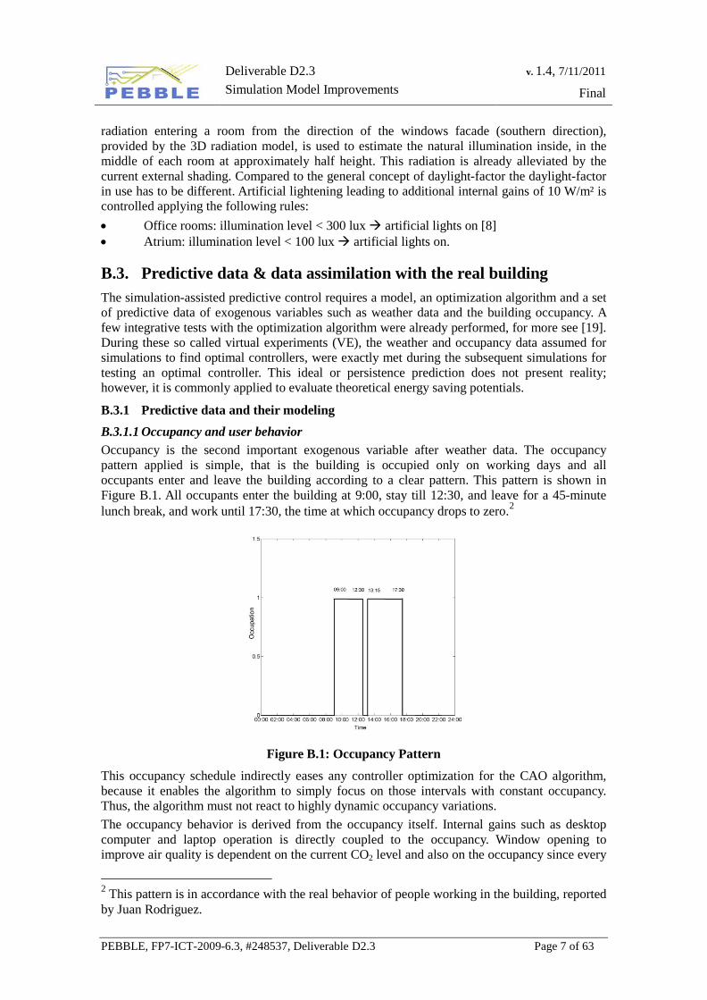
B.3.1 Predictive data and their modeling B.3.1.1 Occupancy and user behavior Occupancy is the second important exogenous variable after weather data. The occupancy pattern applied is simple, that is the building is occupied only on working days and all occupants enter and leave the building according to a clear pattern. This pattern is shown in Figure B.1. All occupants enter the building at 9:00, stay till 12:30, and leave for a 45-minute lunch break, and work until 17:30, the time at which occupancy drops to zero.2
Figure B.1: Occupancy Pattern
This occupancy schedule indirectly eases any controller optimization for the CAO algorithm, because it enables the algorithm to simply focus on those intervals with constant occupancy. Thus, the algorithm must not react to highly dynamic occupancy variations. The occupancy behavior is derived from the occupancy itself. Internal gains such as desktop computer and laptop operation is directly coupled to the occupancy. Window opening to improve air quality is dependent on the current CO2 level and also on the occupancy since every
2 This pattern is in accordance with the real behavior of people working in the building, reported by Juan Rodriguez.
Deliverable D2.3 Simulation Model Improvements
v. 1.4, 7/11/2011
Final
PEBBLE, FP7-ICT-2009-6.3, #248537, Deliverable D2.3 Page 8 of 63
occupant increases the CO2 level, see B.2.3. During periods with occupancy, artificial lightening gains are switched on and off depending on the illumination in the room, see B.2.3.2. B.3.1.2 Weather data Weather data represent the most crucial exogenous variable in the predictive control scheme. Supply with accurate real weather forecast data is not been realized in the current project. In [9] numerical weather data from COSMO-7 (a numerical weather prediction model) have been used for weather prediction, which was updated every 12 hours for a horizon of three days. Local mean anomalies were corrected using a linear Kalman filter, incorporating on-site weather measurements. Predictive control with persistence weather predictions (tomorrow as today) clearly showed less Non Renewable Primary Energy (NRPE) saving potential than predictive control with real weather predictions; the respective additional NRPE use with respect to a performance bound (PB), has been found to be more than twice with persistence predictions. For details on weather predictions see [4, 12, 13] and especially in the context of building simulation see [14]. Incorporation of weather data as described above requires collaboration with a local meteorological institute. This was not considered in the beginning. Ideally, an additional locally installed weather station is utilized to make correlation calculations and calibrate the forecast data from the local institute for the site. Since none of the consortium partner can cover the topic weather forecast as described in the first paragraph the only remaining solution is persistence prediction. Weather data for the building in Kassel are recorded at site and saved in a database to be supplied for simulations. The weather data comprises information on air temperature and –pressure, wind speed and -direction, relative humidity, global and diffuse –radiation. When deciding upon the control strategy for the next day, the measured weather data from the previous day before shall be used.
B.3.2 Model assimilation Reliable and accurate enough results for the continuous building simulation, evoked by the optimization algorithm of the predictive control see [19], depend on two things, first the building model itself with all needed parameters, and second, the initial conditions of the building model. The building model and the validation of the model reported in the former deliverable [5] misses the model assimilation procedure, which is discussed herein. B.3.2.1 Initial Conditions and settling phase Assume a controller design for the next day (control horizon = 24 hours) given a prediction horizon of one day (prediction horizon = 24 hours). The building state at the beginning of the next day (the beginning of the next control horizon) must be approximated to guarantee according initial conditions. One approach is to prepend the simulation period (prediction horizon) by a so called settling phase and use past measurement results to thermally adjust the building model to the current stage. This could be done with an increases time step to limit the calculation time. Another suitable and less calculation time consuming approach is employment of initial conditions for the thermal masses. These conditions could be generated from past measurement results from sensors in the real building. Variations of the model output due to inaccurate initial conditions increase the scenario uncertainties. Ideally, the building simulation period is not greater than the prediction horizon in order to keep the calculation time low; however, this is only possible if initial conditions of thermal masses from the building model can be set directly for the used simulation software. Although, this procedure is an approximation, because in reality the thermal building masses never show a uniform temperature profile, it is assumed that averaged values from that past will lead to suitable initial conditions, but this would require a detailed investigation. There exists a problem of heterogeneity between the measurement data available from building sensors, and internal states provided by the building simulation environment. Harmonizing this
Deliverable D2.3 Simulation Model Improvements
v. 1.4, 7/11/2011
Final
PEBBLE, FP7-ICT-2009-6.3, #248537, Deliverable D2.3 Page 9 of 63
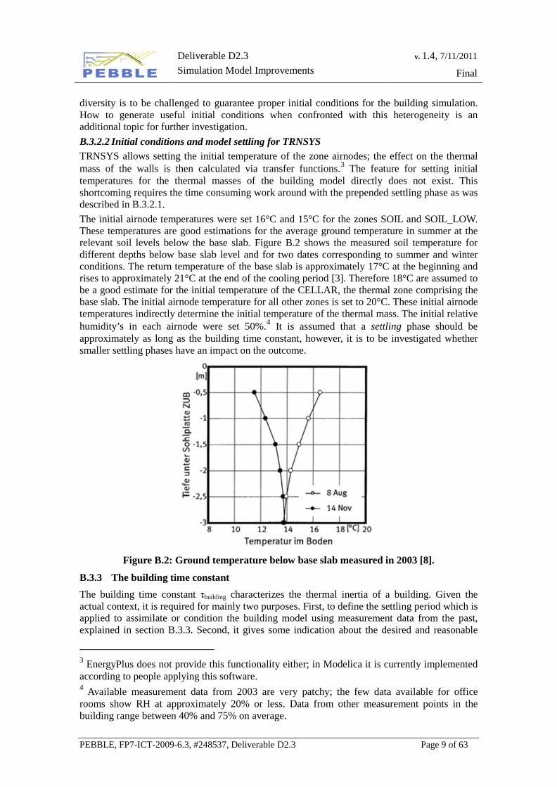
diversity is to be challenged to guarantee proper initial conditions for the building simulation. How to generate useful initial conditions when confronted with this heterogeneity is an additional topic for further investigation. B.3.2.2 Initial conditions and model settling for TRNSYS TRNSYS allows setting the initial temperature of the zone airnodes; the effect on the thermal mass of the walls is then calculated via transfer functions.3 The feature for setting initial temperatures for the thermal masses of the building model directly does not exist. This shortcoming requires the time consuming work around with the prepended settling phase as was described in B.3.2.1. The initial airnode temperatures were set 16°C and 15°C for the zones SOIL and SOIL_LOW. These temperatures are good estimations for the average ground temperature in summer at the relevant soil levels below the base slab. Figure B.2 shows the measured soil temperature for different depths below base slab level and for two dates corresponding to summer and winter conditions. The return temperature of the base slab is approximately 17°C at the beginning and rises to approximately 21°C at the end of the cooling period [3]. Therefore 18°C are assumed to be a good estimate for the initial temperature of the CELLAR, the thermal zone comprising the base slab. The initial airnode temperature for all other zones is set to 20°C. These initial airnode temperatures indirectly determine the initial temperature of the thermal mass. The initial relative humidity’s in each airnode were set 50%.4 It is assumed that a settling phase should be approximately as long as the building time constant, however, it is to be investigated whether smaller settling phases have an impact on the outcome.
Figure B.2: Ground temperature below base slab measured in 2003 [8].
B.3.3 The building time constant The building time constant τbuilding characterizes the thermal inertia of a building. Given the actual context, it is required for mainly two purposes. First, to define the settling period which is applied to assimilate or condition the building model using measurement data from the past, explained in section B.3.3. Second, it gives some indication about the desired and reasonable
3 EnergyPlus does not provide this functionality either; in Modelica it is currently implemented according to people applying this software. 4 Available measurement data from 2003 are very patchy; the few data available for office rooms show RH at approximately 20% or less. Data from other measurement points in the building range between 40% and 75% on average.
Deliverable D2.3 Simulation Model Improvements
v. 1.4, 7/11/2011
Final
PEBBLE, FP7-ICT-2009-6.3, #248537, Deliverable D2.3 Page 10 of 63
prediction horizon of the MPC scheme. B.3.3.1 Measuring of the building time constant As in classical control theory this time constant may be measured applying a temperature step function:
𝑓(𝑡) = Θ�𝑡𝑠𝑡𝑒𝑝� ∗ 𝑇Θ; Θ is the step function and 𝑇Θ the upper set temperature. This could be realized via heating of a “test-room” until the relevant building volume has reached the temperature 𝑇Θ > 𝑇�𝑎𝑚𝑏𝑖𝑒𝑛𝑡, to assure defined initial conditions. Subsequently, the time-development of the temperature must be recorded while the “test-room” is free floating, i.e. it is necessary to exclude additional heating or cooling. Real measurement of the building time constant is a challenging and energy consuming endeavor, in fact it is not performable. Uncertainties involved are all external variables such as the weather conditions, the internal gains and the occupancy behavior. One approach to obtain this constant is to calculate it analytically but this requires many other constants, part of which is not known. Virtual measuring of τbuilding using simulations is less demanding than real measuring. The constant can be measured only indirectly via the temperature, which changes continuously due to interaction with the environment making it difficult to define constant boundary conditions. Because these are never constant in reality, natural weather data are used instead of artificial ambient boundary conditions. Literature values from practice for τbuilding can be used for comparison with obtained results. A typical value for heavy weight construction is 100 hours, for measurement procedure compare also with [7] (52 et seqq.), [1] (p. 26). The definition of τbuilding according to [15, 16] is
𝜏𝑏𝑢𝑖𝑙𝑑𝑖𝑛𝑔 =𝐶
𝐿𝑇 + 𝐿𝑉 ;
here 𝐶 is the effective heat capacitance of the building, 𝐿𝑇 is the transmission conductance and 𝐿𝑉 is the ventilation conductance. Subsequently, measuring of τbuilding for the Tower, the simplified building model of the building in Kassel is conducted. This is done using TRNSYS and real weather data from 2003. B.3.3.2 General simulation parameters To measure τbuilding a certain simulation interval in winter of 2003 was picked. In this computer experiment the settling phase is to heat up the test rooms to a certain temperature, then the test rooms are switched to free floating and the temperature transient is recorded.
• Time interval [289,2000] in hours or [13th January 0:00, 25th March 07:00] • Step size = 1 h • Settling period: 200 h, ideal heating or cooling to 50°C for the test zones
The set temperature for the three office rooms (R007, R107, and R207) is set to 𝑇Θ= 50°C, for the other zones it is set to the measured values back then in 2003. During the settling period ideal heating or cooling is applied. After the settling, all zones are free floating. The conditions during this time are given below. B.3.3.3 Conditions and analysis for free floating and empty building Interaction of the building is only due to the internal gains given below and the prevalent weather data. • Shading completely open • Internal gains:
o CELLAR: 4 x 150 W (server room) o Constant conditions: AT009, AT109, AT209: each 250/3 W = 83.33 W; o Occupancy = 0, no natural or mechanical ventilation
Deliverable D2.3 Simulation Model Improvements
v. 1.4, 7/11/2011
Final
PEBBLE, FP7-ICT-2009-6.3, #248537, Deliverable D2.3 Page 11 of 63
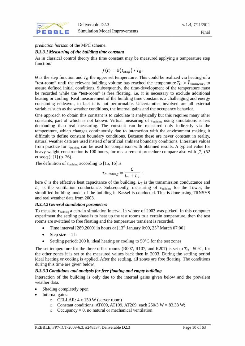
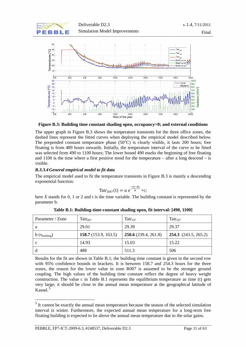
Figure B.3: Building time constant shading open, occupancy=0; and external conditions
The upper graph in Figure B.3 shows the temperature transients for the three office zones, the dashed lines represent the fitted curves when deploying the empirical model described below. The prepended constant temperature phase (50°C) is clearly visible, it lasts 200 hours; free floating is from 489 hours onwards. Initially, the temperature interval of the curve to be fitted was selected from 490 to 1100 hours; The lower bound 490 marks the beginning of free floating and 1100 is the time where a first positive trend for the temperature – after a long descend – is visible. B.3.3.4 General empirical model to fit data The empirical model used to fit the temperature transients in Figure B.3 is mainly a descending exponential function:
Tair𝑋07(t) = 𝑎 𝑒−(t−d)
𝑏 +c; here X stands for 0, 1 or 2 and t is the time variable. The building constant is represented by the parameter b.
Table B.1: Building-time-constant shading open, fit interval: [490, 1100]
Parameter / Zone Tair007 Tair107 Tair207
a 29.01 29.39 29.37
b (τbuilding) 158.7 (153.9, 163.5) 250.6 (239.4, 261.8) 254.3 (243.5, 265.2)
c 14.93 15.03 15.22
d 488 511.3 506
Results for the fit are shown in Table B.1; the building time constant is given in the second row with 95% confidence bounds in brackets. It is between 158.7 and 254.3 hours for the three zones, the reason for the lower value in zone R007 is assumed to be the stronger ground coupling. The high values of the building time constant reflect the degree of heavy weight construction. The value c in Table B.1 represents the equilibrium temperature as time (t) gets very large; it should be close to the annual mean temperature at the geographical latitude of Kassel.5
5 It cannot be exactly the annual mean temperature because the season of the selected simulation interval is winter. Furthermore, the expected annual mean temperature for a long-term free floating building is expected to lie above the annual mean temperature due to the solar gains.
Deliverable D2.3 Simulation Model Improvements
v. 1.4, 7/11/2011
Final
PEBBLE, FP7-ICT-2009-6.3, #248537, Deliverable D2.3 Page 12 of 63
B.3.3.5 Further simulation results for the building time constant and interpretation In addition to the reported results, simulation experiments with minor variations provide further results for discussion. Detailed results can be found in Appendix 1. Because it is not straight forward to decide at which point in time the positive temperature trend after the continuous descend starts, an additional fit with an altered interval was conducted. Reduction of the fit interval to [490-1000] leads to τbuilding of 171, 327 and 332 hours for the three zones, respectively. This equals an increase of τbuilding between approximately 8 and 30%. In the analysis above the occupancy was neglected; however, simulation experiments with occupancy don’t change the results remarkably. This might be because higher internal gains, and window opening to keep CO2 levels acceptable, compensate each other to some degree. Entirely closed shading happens to increase τbuilding by approximates 5-10% which is not what was intuitively expected. Comparison of the results with other simulation results relating to the building in Kassel in [7] (page 54, τbuilding estimated is 140 h) shows, that the found range for τbuilding is valid. However, the results in [7] refer to moderate night ventilation, compared to very low thermal coupling prevalent for results found herein. The building time constant is by far greater than the reliable period for weather forecast data. Thus, the constraint to define a reasonable prediction horizon is given by the reliability of the weather predictions, rather than the building time constant.
B.4. Model complexity and calculation time The building model design, parameters and the validation of the model were dealt with in the former deliverable [5]. The data involved in the building simulation and model assimilation is discussed in 0. This section describes the complexity of the building model in TRNSYS and reports on the calculation time.
B.4.1 Embedded MATLAB (Type155) in TRNSYS The general Type to be used for any building simulation in TRNSYS is Type56. A Type in TRNSYS is something like a template or a functional block which requires parameterization. Furthermore, any Type has input and output variables. Input variables for Type56 are for example mass flow rates, set temperatures, climate data etc., and output variables are for example energy consumption, actual temperature, CO2 level concentration, etc. Many repeatedly existing input variables (mass flow rate, internal gains, clothing factor, etc.) have to be controlled depending on other variables. MATLAB is predestined to be used for this task which requires a modular approach. B.4.1.1 Shared functionality and controllers in the building model The building model (the TRNSYS simulation) comprises two parts, the building model itself – passive devices such as walls and roofs – and active devices such as TABS and operable windows compare with [6]. Controls related to active devices being part of the model require input variables. Active and passive devices from Type56 generate output variables. The Tower model comprises nine thermal zones; a few zones have only passive devices but some have passive and active devices. Each active device requires a control. These controls could be assembled in TRNSYS using a number of Types for each active device. Although similar control tasks may exist, each active device requires its own controller. This fact is unpleasant for flexibility and an extension of the model. Vector and matrix elements in MATLAB provide an elegant way to solve multiple but similar control tasks. Further, the possibility for quick extension or modification of the initially simplified big building model, was a major constraint when designing controls and providing initial parameters for the building model. Because MATLAB provides the optimal solution to simply handle and extend the mentioned control tasks, a MATLAB instance embedded in TRNSYS is used. This is depicted in Figure B.4. The details about the applied modular approach to handle input- and output- connection for the embedded MATLAB instance is
Deliverable D2.3 Simulation Model Improvements
v. 1.4, 7/11/2011
Final
PEBBLE, FP7-ICT-2009-6.3, #248537, Deliverable D2.3 Page 13 of 63
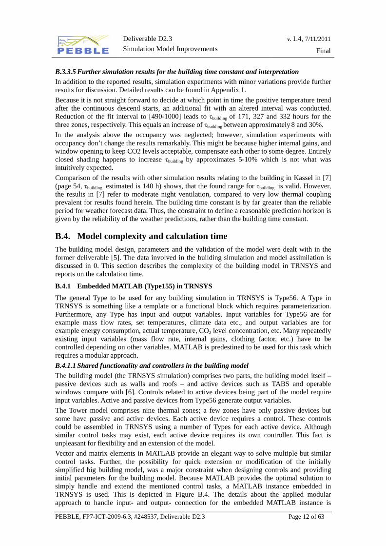
described in detail in the next subsection. B.4.1.2 Characteristic zones and interface with MATLAB The majority of functionality related to controlling of devices being part of the building is realized in MATLAB because it provides an elegant way to solve multiple but similar control tasks. The lower part in Figure B.4 shows the embedded MATLAB instance being part of the TRNSYS simulation; compare also with Figure B.8. The TRNSYS Type155 – which is essentially a functional block with inputs and outputs in TRNSYS – enables the connection between TRNSYS and MATLAB. A MATLAB script file is defined in Type155. This script has its own workspace and an input and output array, serving as interface between the pure TRNSYS environment and MATLAB. The input and output arrays correspond with the inputs and outputs of the TRNSYS Type155.
MATLAB environment
MATLAB (instance 2)
Weather data
Type155-control
Type56-TRNFLOW
Lnterface Basement
Lnterface Atrium
Lnterface hffice
from TRNSYS
to TRNSYS
Output data R107
Input data R107
Figure B.4: Modular zone interface between MATLAB and TRNSYS Type155
To connect the embedded MATLAB (Type155) efficiently with Type56 a structured approach is needed. Three scaffoldings, in terms of relevant input and output parameters and variables were predefined as thermal zones: a Basement-, an Atrium, and an Office zone I/O interface. Each thermal zone of the building was assigned one of these three I/O interfaces. This modular interface concept is shown in Figure B.4 for two thermal zones. The upper small arrow pointing to the right corner of the rectangle “Lnterface Basement” represents Input data from TRNSYS for a basement zone, the arrow leaving this rectangle represents the Output data from MATLAB to TRNSYS for this thermal zone. Similarly Input and Output data exchange is depicted for an Office zone “Lnterface hffice”. The gray area of the rectangles represents data manipulation and output data generation, e.g. a predefined set temperature for a thermal zone and the actual room temperature from the input data of this zone are used to determine the mass flow rate of the floor heating, this flow rate is sent as output back to TRNSYS. This modular interface concept allows for systematic and structured extension from the Tower to a model similar to it, or to the big building model with more thermal zones. Further, it provides a certain standardized interface for thermal zones between TRNSYS and MATLAB for future work.
B.4.2 Calculation time Simulation run-time of the building simulation depends on a few circumstances:
Deliverable D2.3 Simulation Model Improvements
v. 1.4, 7/11/2011
Final
PEBBLE, FP7-ICT-2009-6.3, #248537, Deliverable D2.3 Page 14 of 63
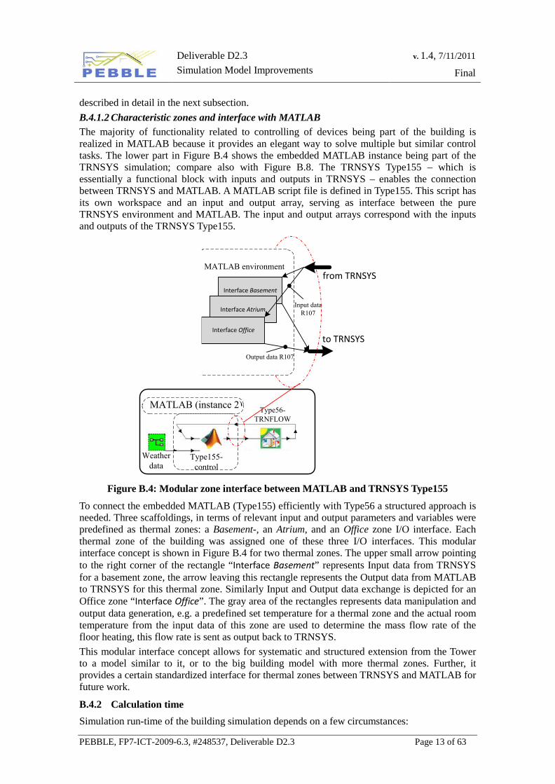
• CPU and Memory performance • Prediction horizon • Model complexity • Model assimilation procedure The first point refers to financial issues and developments in the computer hardware sector. In general, a reasonable prediction horizon will be chosen, first, dependent on the thermal building time constant and second, restricted by the accuracy of weather predictions. However, any prediction accuracy of relevant exogenous conditions will naturally limit the prediction horizon via their decreasing accuracy as the prediction horizon increases. The model complexity is closely linked to the required accuracy and reliability of the results for energy demand, level of comfort, etc. The optimal trade-off between model complexity and accuracy of simulation results has to be found. At current stage there is still an optimization potential, that is, it is assumed that the model complexity can be reduced; to which degree requires more detailed analysis. Actually the model assimilation procedure, compare with 0, requires a great deal of calculation time in the TRNSYS building simulation. B.4.2.1 Report on the calculation time of the building simulation Figure B.5 shows the TRNSYS Calculation Time on the vertical axis against the simulation Time Step on the horizontal axis, for a simulation of the Tower over an interval of four and seven days (96 hours and 168 hours). Error bars shown refer to 3%, found after repeated simulations. When including a prepended settling phase as discussed in 0 a minimum simulation period of 168 hours is assumed to be required. The three curves in Figure B.5 are smoothed polygons. The basis data of these curves show the calculation time dependency on the Time Step. The blue and the red line show the total TRNSYS calculation time for a simulation interval of 96 and 168 hours. For 168 hours an additional simulation series was conducted, with detailed short wave radiation mode switched on in all relevant zones in TRNSYS. The impact of the detailed model becomes clearly visible for a Time Step of 0.125 hours. For all curves there is a strong dependence on the Time Step. Data source for the calculation time was the list file, which is an automatically generated file after a TRNSYS simulation. The list file is an execution report; it contains all generated TRNSYS messages and is the first place to check when the simulation fails to run. In addition, it provides information about the initial parameters such as start and stop time and the Time Step and a detailed report on the total TRNSYS Calculation Time.
Figure B.5: Simulation performance, total TRNSYS calculation time
Deliverable D2.3 Simulation Model Improvements
v. 1.4, 7/11/2011
Final
PEBBLE, FP7-ICT-2009-6.3, #248537, Deliverable D2.3 Page 15 of 63
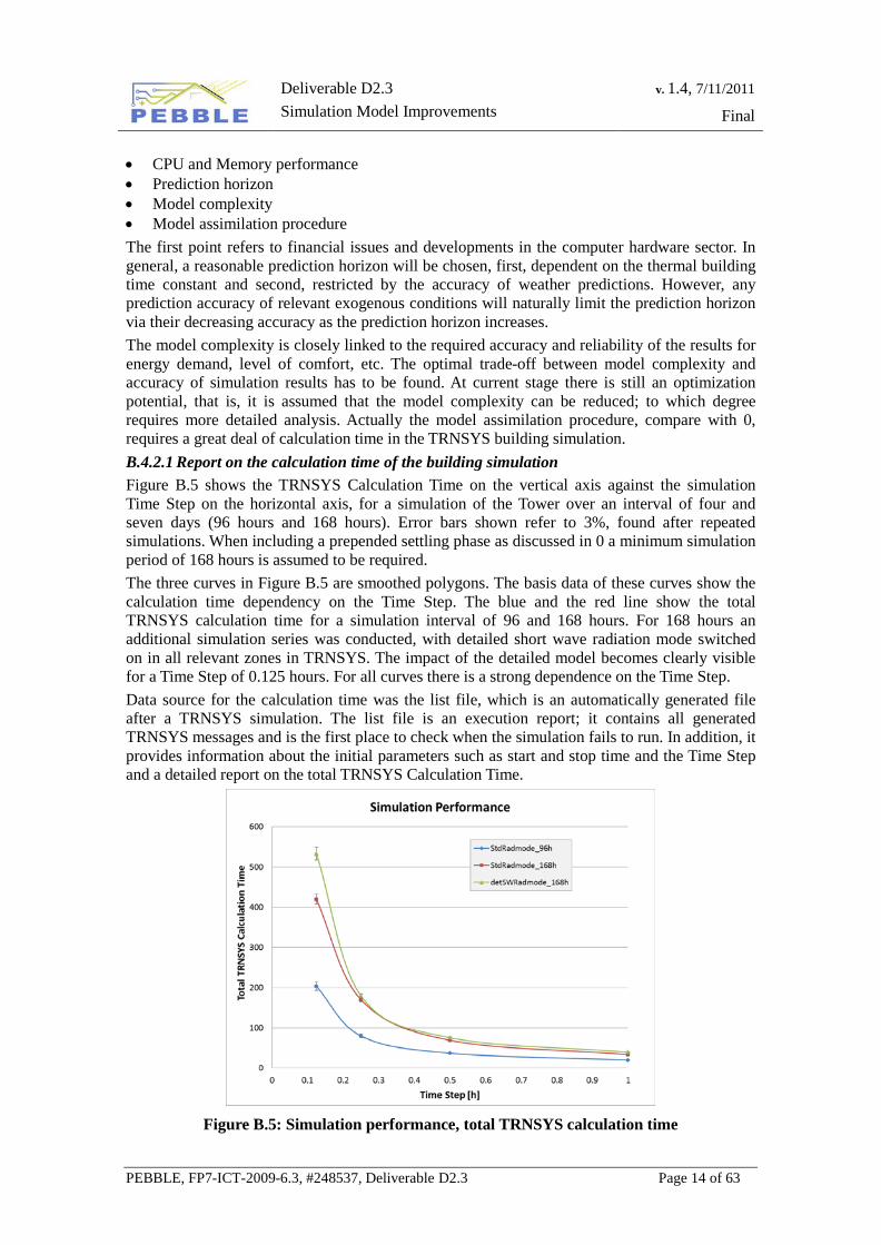
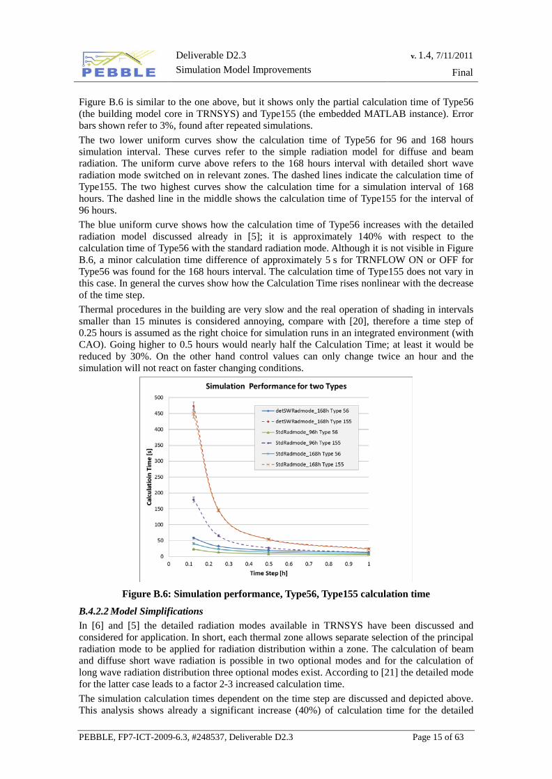
Figure B.6 is similar to the one above, but it shows only the partial calculation time of Type56 (the building model core in TRNSYS) and Type155 (the embedded MATLAB instance). Error bars shown refer to 3%, found after repeated simulations. The two lower uniform curves show the calculation time of Type56 for 96 and 168 hours simulation interval. These curves refer to the simple radiation model for diffuse and beam radiation. The uniform curve above refers to the 168 hours interval with detailed short wave radiation mode switched on in relevant zones. The dashed lines indicate the calculation time of Type155. The two highest curves show the calculation time for a simulation interval of 168 hours. The dashed line in the middle shows the calculation time of Type155 for the interval of 96 hours. The blue uniform curve shows how the calculation time of Type56 increases with the detailed radiation model discussed already in [5]; it is approximately 140% with respect to the calculation time of Type56 with the standard radiation mode. Although it is not visible in Figure B.6, a minor calculation time difference of approximately 5 s for TRNFLOW ON or OFF for Type56 was found for the 168 hours interval. The calculation time of Type155 does not vary in this case. In general the curves show how the Calculation Time rises nonlinear with the decrease of the time step. Thermal procedures in the building are very slow and the real operation of shading in intervals smaller than 15 minutes is considered annoying, compare with [20], therefore a time step of 0.25 hours is assumed as the right choice for simulation runs in an integrated environment (with CAO). Going higher to 0.5 hours would nearly half the Calculation Time; at least it would be reduced by 30%. On the other hand control values can only change twice an hour and the simulation will not react on faster changing conditions.
Figure B.6: Simulation performance, Type56, Type155 calculation time
B.4.2.2 Model Simplifications In [6] and [5] the detailed radiation modes available in TRNSYS have been discussed and considered for application. In short, each thermal zone allows separate selection of the principal radiation mode to be applied for radiation distribution within a zone. The calculation of beam and diffuse short wave radiation is possible in two optional modes and for the calculation of long wave radiation distribution three optional modes exist. According to [21] the detailed mode for the latter case leads to a factor 2-3 increased calculation time. The simulation calculation times dependent on the time step are discussed and depicted above. This analysis shows already a significant increase (40%) of calculation time for the detailed
Deliverable D2.3 Simulation Model Improvements
v. 1.4, 7/11/2011
Final
PEBBLE, FP7-ICT-2009-6.3, #248537, Deliverable D2.3 Page 16 of 63
short wave radiation mode compared to the standard mode. The detailed long wave mode, for which an even higher calculation time increase is expected, was not analyzed. It is only required for location dependent comfort evaluation and this degree of detail is not necessary in the given case. The intention to keep the calculation time low and reduce it if possible, and the limited advantages of the detailed radiation modes for the purpose of the building model lead to the decision to disregard the detailed modes. B.4.2.3 Parameter importance A general question is: how does any parameter uncertainty propagate through the model? This relative contribution of a parameter uncertainty to the model output leads to the importance of a parameter. Via a ranking of the importance of a parameter it will be possible to classify parameters according to their relevance. Subsequently, it will be possible to select parameters requiring attention for individual adaption, if the concept is applied to a different building. All the other parameters will be given suitable default values. General sensitivities and a robustness analysis for a rather simple building model used for a MPC controller can be found in [17]. In this research model parameters for window U-values, g-values, and the thermal building mass have been varied by ± 10 %, and wall U-values have been varied by ± 15 %. The impact on the results for energy savings were within a few percentages compared to the undisturbed base case. The impact on the amount of comfort violations was maximum 9%. A detailed analysis of model parameters for a complex model is involved and requires an iterative process which initiates with a first screening process ranking the importance of the different parameters. Following this crude first stage more elaborated techniques may be applied to analyze the model uncertainty [14]. Although the Tower model is already a simplification of a complex building model it sustains a high degree of functional complexity. Therefore, the approach described above was not applied because it is cumbersome and time consuming. The potential results of the described analysis, however, might be of help also for reducing the complexity of the model. In this way a calculation time reduction and isolation of the most important parameters could be achieved. Therefore, this procedure is an interesting subject for future research on applicability and required adaptions of the applied predictive control scheme to different buildings.
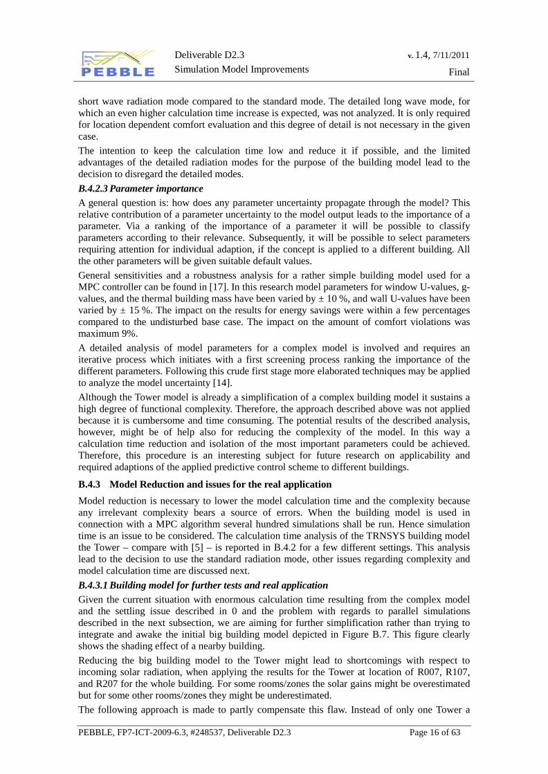
B.4.3 Model Reduction and issues for the real application Model reduction is necessary to lower the model calculation time and the complexity because any irrelevant complexity bears a source of errors. When the building model is used in connection with a MPC algorithm several hundred simulations shall be run. Hence simulation time is an issue to be considered. The calculation time analysis of the TRNSYS building model the Tower – compare with [5] – is reported in B.4.2 for a few different settings. This analysis lead to the decision to use the standard radiation mode, other issues regarding complexity and model calculation time are discussed next. B.4.3.1 Building model for further tests and real application Given the current situation with enormous calculation time resulting from the complex model and the settling issue described in 0 and the problem with regards to parallel simulations described in the next subsection, we are aiming for further simplification rather than trying to integrate and awake the initial big building model depicted in Figure B.7. This figure clearly shows the shading effect of a nearby building. Reducing the big building model to the Tower might lead to shortcomings with respect to incoming solar radiation, when applying the results for the Tower at location of R007, R107, and R207 for the whole building. For some rooms/zones the solar gains might be overestimated but for some other rooms/zones they might be underestimated. The following approach is made to partly compensate this flaw. Instead of only one Tower a
Deliverable D2.3 Simulation Model Improvements
v. 1.4, 7/11/2011
Final
PEBBLE, FP7-ICT-2009-6.3, #248537, Deliverable D2.3 Page 17 of 63
second Tower for the building simulation located towards the western end of the building is incorporated in addition to the existing Tower. These two Towers provide results for a few thermal zones at two slightly different locations, which will be facilitated to derive control schemes for thermal zones that will not be simulated. This can be achieved using according weight factors.
Figure B.7: Shading effect from a nearby building and the concrete construction above the
terrace
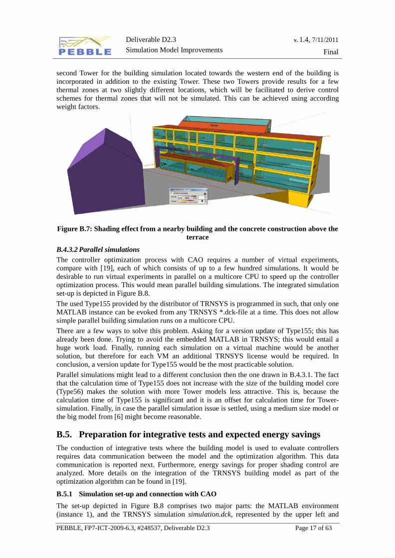
B.4.3.2 Parallel simulations The controller optimization process with CAO requires a number of virtual experiments, compare with [19], each of which consists of up to a few hundred simulations. It would be desirable to run virtual experiments in parallel on a multicore CPU to speed up the controller optimization process. This would mean parallel building simulations. The integrated simulation set-up is depicted in Figure B.8. The used Type155 provided by the distributor of TRNSYS is programmed in such, that only one MATLAB instance can be evoked from any TRNSYS *.dck-file at a time. This does not allow simple parallel building simulation runs on a multicore CPU. There are a few ways to solve this problem. Asking for a version update of Type155; this has already been done. Trying to avoid the embedded MATLAB in TRNSYS; this would entail a huge work load. Finally, running each simulation on a virtual machine would be another solution, but therefore for each VM an additional TRNSYS license would be required. In conclusion, a version update for Type155 would be the most practicable solution. Parallel simulations might lead to a different conclusion then the one drawn in B.4.3.1. The fact that the calculation time of Type155 does not increase with the size of the building model core (Type56) makes the solution with more Tower models less attractive. This is, because the calculation time of Type155 is significant and it is an offset for calculation time for Tower-simulation. Finally, in case the parallel simulation issue is settled, using a medium size model or the big model from [6] might become reasonable.
B.5. Preparation for integrative tests and expected energy savings The conduction of integrative tests where the building model is used to evaluate controllers requires data communication between the model and the optimization algorithm. This data communication is reported next. Furthermore, energy savings for proper shading control are analyzed. More details on the integration of the TRNSYS building model as part of the optimization algorithm can be found in [19].
B.5.1 Simulation set-up and connection with CAO The set-up depicted in Figure B.8 comprises two major parts: the MATLAB environment (instance 1), and the TRNSYS simulation simulation.dck, represented by the upper left and
Deliverable D2.3 Simulation Model Improvements
v. 1.4, 7/11/2011
Final
PEBBLE, FP7-ICT-2009-6.3, #248537, Deliverable D2.3 Page 18 of 63
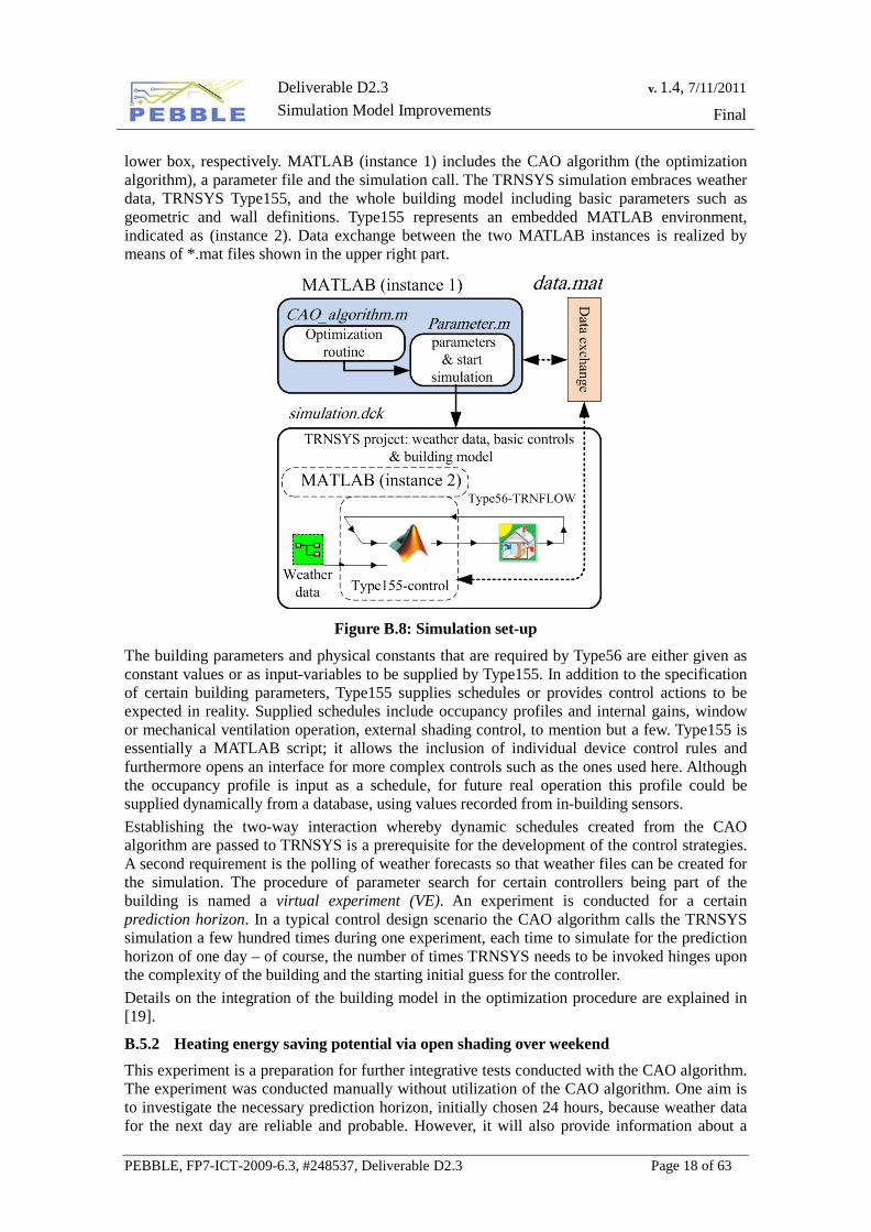
lower box, respectively. MATLAB (instance 1) includes the CAO algorithm (the optimization algorithm), a parameter file and the simulation call. The TRNSYS simulation embraces weather data, TRNSYS Type155, and the whole building model including basic parameters such as geometric and wall definitions. Type155 represents an embedded MATLAB environment, indicated as (instance 2). Data exchange between the two MATLAB instances is realized by means of *.mat files shown in the upper right part.
Figure B.8: Simulation set-up
The building parameters and physical constants that are required by Type56 are either given as constant values or as input-variables to be supplied by Type155. In addition to the specification of certain building parameters, Type155 supplies schedules or provides control actions to be expected in reality. Supplied schedules include occupancy profiles and internal gains, window or mechanical ventilation operation, external shading control, to mention but a few. Type155 is essentially a MATLAB script; it allows the inclusion of individual device control rules and furthermore opens an interface for more complex controls such as the ones used here. Although the occupancy profile is input as a schedule, for future real operation this profile could be supplied dynamically from a database, using values recorded from in-building sensors. Establishing the two-way interaction whereby dynamic schedules created from the CAO algorithm are passed to TRNSYS is a prerequisite for the development of the control strategies. A second requirement is the polling of weather forecasts so that weather files can be created for the simulation. The procedure of parameter search for certain controllers being part of the building is named a virtual experiment (VE). An experiment is conducted for a certain prediction horizon. In a typical control design scenario the CAO algorithm calls the TRNSYS simulation a few hundred times during one experiment, each time to simulate for the prediction horizon of one day – of course, the number of times TRNSYS needs to be invoked hinges upon the complexity of the building and the starting initial guess for the controller. Details on the integration of the building model in the optimization procedure are explained in [19].
B.5.2 Heating energy saving potential via open shading over weekend This experiment is a preparation for further integrative tests conducted with the CAO algorithm. The experiment was conducted manually without utilization of the CAO algorithm. One aim is to investigate the necessary prediction horizon, initially chosen 24 hours, because weather data for the next day are reliable and probable. However, it will also provide information about a
Deliverable D2.3 Simulation Model Improvements
v. 1.4, 7/11/2011
Final
PEBBLE, FP7-ICT-2009-6.3, #248537, Deliverable D2.3 Page 19 of 63
theoretical energy saving potential in the heating period as is explained next. In the following experiment the potential heating energy savings for proper shading control is examined in a simple way. Assume a sunny bank holiday or weekend in the heating period with no occupancy. Practically it can happen that shading without elaborated automatic control mechanisms is closed over the weekend for certain rooms. The impact, in terms of missed solar radiation as potential thermal heat source to the building increases with the window fraction of a building. For the ZUB building in Kassel, the fraction of south facing windows is extremely high and therefore it is crucial to operate the shading accordingly. The potential saving of energy was obtained by taking the difference between a base case and a simulation with varied values for the shading variable. In total three scenarios were investigated and are explained in detail in B.5.2.2. B.5.2.1 General conditions The general conditions for this analysis include a settling period which is followed by a measuring period. The length of these periods and other conditions are as follows: • Settling period 168 hours [1537-1704], to measured temperatures (ideal heating/cooling) • Measuring period [1705-1824] (the time after settling) • Set temperature heating in measuring period = 21°C in zone R007, R107, R207 (ideal
heating, no cooling) • Occupancy such as in Figure B.1 • Climate data are real weather data from 2003 in Kassel, Figure B.9. graph (a) B.5.2.2 Scenarios and calculation of the energy savings Three different scenarios were investigated. In order to find a theoretical heating energy saving potential a base case simulation and a second simulation with different shading operation were conducted for each scenario. The major difference between any base case and the additional simulation is the shading parameter. • Shading CLOSED = additional extinction of solar radiation by 70% • Shading OPEN = no additional extinction Calculation of the potential energy savings is exemplified for the first scenario: For the base case, shading was OPEN the whole measuring period; during the second simulation it was CLOSED for the measuring period. Subtracting the heating energy demand of this simulation from the demand of the base case leads to the result shown in Figure B.9 (b). Results for the other scenarios are obtained in a similar way, but the OPEN/CLOSED periods given in the list below are different. While for the first and the second scenario heating is continuously in operation, it is interrupted during the “virtual weekend” for the third scenario. 1. Scenario; potential heating energy savings shows plot (b)
Base case: Continuous heating to 21°C and shading completely OPEN for the measuring period. Variation for the second simulation: shading completely CLOSED for the measuring period.
2. Scenario; potential heating energy savings shows Plot (c) Base case: Continuous heating to 21°C and shading completely OPEN for the measuring period. Variation for the second simulation: shading CLOSED for the “virtual weekend”.
3. Scenario; potential heating energy savings shows Plot (d) Base case: Continuous heating to 21°C during the measuring period except for the “virtual weekend” which is free floating, shading completely OPEN for the measuring period. Variation for the second simulation: shading CLOSED for the “virtual weekend”.
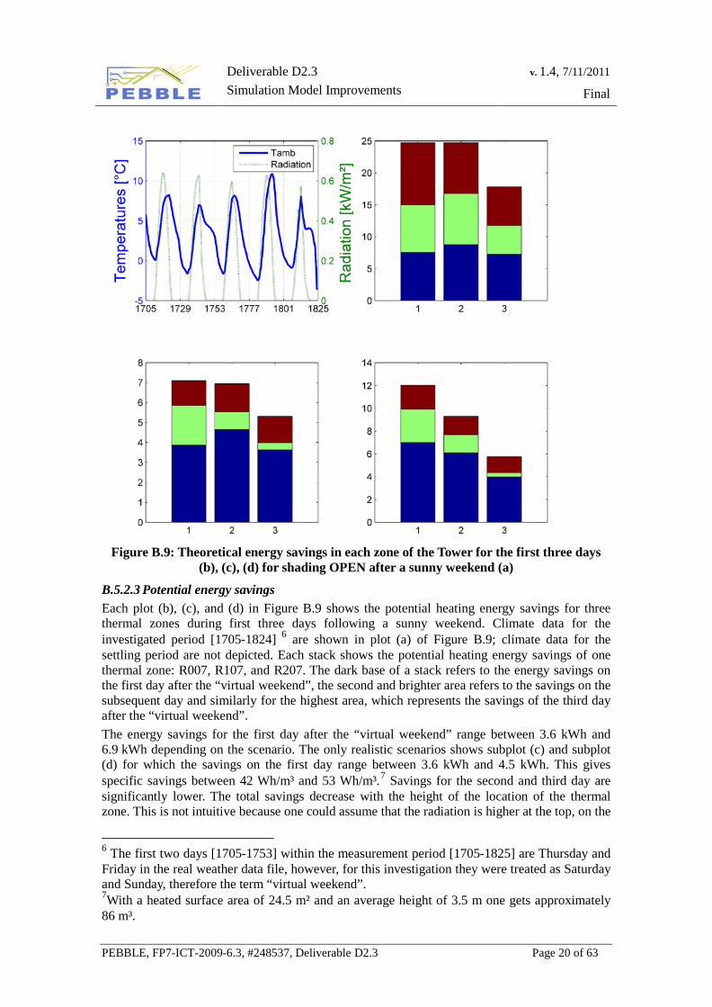
Deliverable D2.3 Simulation Model Improvements
v. 1.4, 7/11/2011
Final
PEBBLE, FP7-ICT-2009-6.3, #248537, Deliverable D2.3 Page 20 of 63
Figure B.9: Theoretical energy savings in each zone of the Tower for the first three days
(b), (c), (d) for shading OPEN after a sunny weekend (a)
B.5.2.3 Potential energy savings Each plot (b), (c), and (d) in Figure B.9 shows the potential heating energy savings for three thermal zones during first three days following a sunny weekend. Climate data for the investigated period [1705-1824] 6 are shown in plot (a) of Figure B.9; climate data for the settling period are not depicted. Each stack shows the potential heating energy savings of one thermal zone: R007, R107, and R207. The dark base of a stack refers to the energy savings on the first day after the “virtual weekend”, the second and brighter area refers to the savings on the subsequent day and similarly for the highest area, which represents the savings of the third day after the “virtual weekend”. The energy savings for the first day after the “virtual weekend” range between 3.6 kWh and 6.9 kWh depending on the scenario. The only realistic scenarios shows subplot (c) and subplot (d) for which the savings on the first day range between 3.6 kWh and 4.5 kWh. This gives specific savings between 42 Wh/m³ and 53 Wh/m³.7 Savings for the second and third day are significantly lower. The total savings decrease with the height of the location of the thermal zone. This is not intuitive because one could assume that the radiation is higher at the top, on the
6 The first two days [1705-1753] within the measurement period [1705-1825] are Thursday and Friday in the real weather data file, however, for this investigation they were treated as Saturday and Sunday, therefore the term “virtual weekend”. 7With a heated surface area of 24.5 m² and an average height of 3.5 m one gets approximately 86 m³.
Deliverable D2.3 Simulation Model Improvements
v. 1.4, 7/11/2011
Final
PEBBLE, FP7-ICT-2009-6.3, #248537, Deliverable D2.3 Page 21 of 63
other hand heat transfer from the lower floor to the top floor could overcompensate this effect. The dependence of the heating load on the global radiation has been reported also in [9]. A prediction horizon of at least 48 hours would be the prerequisite to benefit partly from these potential energy savings; however, 72 hours would be desirable. This way the optimization algorithm could design a controller, acting as is described for the first or the second scenario. Assume this is the case, the maximum achievable energy savings for the first three days are shown in graph (c) or (d), depending on whether heating is on or off over the weekend. These saving are obtained for ideal weather prediction; with real weather forecast data the savings will be lower. However, these results give evidence how important an automated operation of shading devices can be.
B.6. Summary and conclusion In B.2 minor changes and refinements made in the modeling of the physical building in Kassel are reported. Refinements are the modeling of manual window opening dependent on varying CO2 levels due to human respiration, and the estimation of natural internal illumination and derived additional internal gains caused by possible artificial lightening. Predictive data for the real building address an important part in this report. A simple occupancy schedule was introduced which should ease the controller design. The forecast weather data supply is very basic, compared to other research projects dealing with predictive and model based controller design. However, given the actual equipment at site persistence prediction is the best possible solution, since the required framework for optimal provision with forecast weather data at site, was not foreseen even in the project proposal. For any future work, in the context of predictive controller design for buildings, the establishment of a universal interface with a local meteorological institute must be considered. The topic model assimilation untouched so far, turns out to be crucial. Compared to building simulations for other purposes an additional difficulty is the continuously required assimilation with new measurement data from the real building. The building time constant provides an estimation of how long the procedure of assimilation via a prepended settling period has to last. The other optional way to assimilate the building via initial values for the thermal masses is currently not possible in TRNSYS. Data availability and heterogeneity between real sensor values and values available from the model make it impossible to conclude anything with regards to the impact on the accuracy now. The settling interval for the building in Kassel should be ideally 168 hours. An interface to tackle simulation of complex buildings with many similar zones was explained in B.4. The modular concept of this interface provides a flexible solution for modification of any building model. The calculation time analysis led to the decision to use a time step of 0.25 hours (maximum 0.5 hours) and the standard radiation mode during simulations. It showed relatively high calculation times for Type155, the embedded MATLAB environment. This indicates that the MATLAB source code should be improved if possible. The influence of TRNFLOW on the calculation time can be neglected. There are three options now for the model to be applied for the real application. The concept with one or two towers or an extended model very similar to the big building model might be used. Which one to use, depends on a solution with regards to parallel simulation. So far only the Tower model can be used, but even in this case parallel simulations are desirable. In B.5 the simulation set-up in connection with CAO was explained, more details on that can be found in [19]. First tests considering possible solutions of CAO but without application of CAO indicated possible energy savings and gave an idea how long to choose the prediction horizon. The results for optimal shading control over a sunny weekend are a theoretical heating energy saving potential of approximately 47 Wh/m³ on Monday. This result indicates a prediction horizon of 72 hours could be reasonable; however, the accuracy of forecast weather data decreases with time. Since persistence predictions are used in the current project 24 hours are sufficient.
Deliverable D2.3 Simulation Model Improvements
v. 1.4, 7/11/2011
Final
PEBBLE, FP7-ICT-2009-6.3, #248537, Deliverable D2.3 Page 22 of 63
References [1] Barbara Beigelböck. Abschätzung des energieeinsparungspotentials durch simulation einer raumtemperaturregelung mit hilfe von modellbasierten prädiktiven regelalgorithmen unter verwendung einer idealen wettervorhersage. Master’s thesis, FH Pinkafeld, 2009. [2] T. Braun, A.Röhler gen. Riemer, and F. Weber. Kurzlehrbuch Physiologie. ELSEVIER, 2006. [3] Centre for Sustainable Building. Measurement data for evaluation, 2003. [4] T.G. Doeswijk and K.J. Keesman. IMPROVING LOCAL WEATHER FORECASTS FOR AGRICULTURAL APPLICATIONS. In Proceedings of the Second IASTED International Multi-Conference, SIGNAL AND IMAGE PROCESSING, 2005. [5] Angela Dröscher, Martin Pichler, Hermann Schranzhofer, Ana Constantin, N. Exizidou, G. Giannakis, and D. Rovas. D2.2 Validation Results of the Models (Draft Version). Technical report, 2011. [6] Angela Dröscher, Hermann Schranzhofer, Juan Rodríguez Santiago, Ana Constantin, Rita Streblow, Dirk Müller, N. Exizidou, G. Giannakis, and D. Rovas. D2.1 Integrated Thermal Simulation Models for the Three Buildings. Technical report, 2010. [7] Lucia Ehricke. Rechnerische untersuchung der wirkung einer intensiven nachtlüftung auf das sommerliche wärmeverhalten des bürogebäudes des zentrums für umweltbewusstes bauen. Master’s thesis, Universität Kassel, Universität Kassel Fachgebiete Bauphysik / TGA, Gottschalkstr. 28, 34109 Kassel, März 2003. [8] de Saldanha Michael Sager Christina Hauser Gerd, Hausladen Gerhard. Forscher drin, forschung dran. zentrum für umweltbewusstes bauen - kassel konzept - planung - bau. Technical report, Biologie, Energie, Umwelt BEO, 2002. [9] Rösler Martin Schmidt Dietrich Hauser Gerd, Kaiser Jan. Energetische optimierung, vermessung und dokumentation für das demonstrationsgebäude des zentrums für umweltbewusstes bauen. Technical report, Universität Kassel, Dezember 2004. [10] Schmidt Dietrich Hauser Gerd, Kaiser Jan. Technical measurement investigations of an office building characterised by low energy use and high thermal comfort. 7th Nordic Symposium on Building Physics in the Nordic Countries, Proceedings, page 8, 2005. * very good. [11] K. Katrin Schlegel. Dokumentation und analyse eines innovativen forschungs und demonstrationsgebäudes. Master’s thesis, 2001. [12] Karel J. Keesman, Diederik Peters, and Leo J.S. Lukasse. Optimal climate control of a storage facility using local weather forecasts. Control Engineering Practice, 11:505–516, 2003. [13] L. Lukasse, J. van Maldegem, E. Dierkes, A.J. van der Voort, J. de Kramer-Cuppen, and G. van der Kolk. ANTICIPATING FUTURE WEATHER AND ENERGY TARIFFS FOR OPTIMAL CONTROL OF INDOOR CLIMATE. In International Congress of Refrigeration, 2007, Beijing, 2007. [14] Ali M. Malkawi, Godfried Augenbroe, and et al. Advanced Building Simulation. Spon Press, 2004. [15] ÖNORM. Energieeffizienz von Gebäuden – Berechnung des Heizenergiebedarfs (ISO/DIS 13790:2005), 2005. [16] ÖNORM. Wärmeschutz im Hochbau; Teil 6: Grundlagen und Nachweisverfahren Heizwärmebedarf und Kühlbedarf, 2006. [17] Frauke Oldewurtel, Dimitrios Gyalistras, Markus Gwerder, Colin N. Jones, Alessandra Parisio, Vanessa Stauch, Beat Lehmann, and Manfred Morari. Increasing energy efficiency in building climate control using weather forecasts and model predictive control. 2010. ***. [18] Dimitrios Rovas. PEBBLE Deliverable 3.2. Technical report, Technical University of

Deliverable D2.3 Simulation Model Improvements
v. 1.4, 7/11/2011
Final
PEBBLE, FP7-ICT-2009-6.3, #248537, Deliverable D2.3 Page 23 of 63
Crete, 2011. [19] Dimitrios Rovas. PEBBLE Deliverable 3.3. Technical report, Technical University of Crete, 2011. [20] Matthias Schuss. Implementation of a predictive simulation-based controller for environmental systems in buildings. PhD thesis, Technische Universität Wien, 2011. [21] TRNSYS Coordinator Thermal Energy System Specialists, LLC 22 North Carroll Street – suite 370 Madison, WI 53703 – U.S.A. A TRaNsient SYstems Simulation Program – TRNSYS 17.00.0019, 2010.
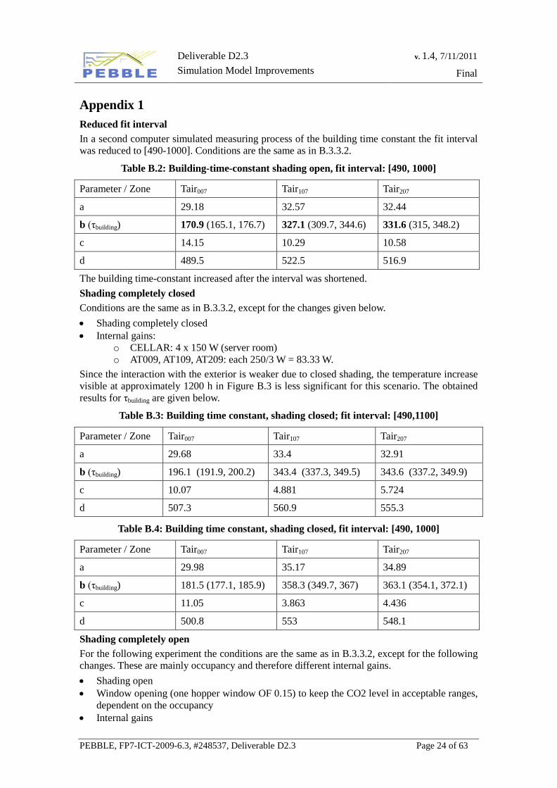
Deliverable D2.3 Simulation Model Improvements
v. 1.4, 7/11/2011
Final
PEBBLE, FP7-ICT-2009-6.3, #248537, Deliverable D2.3 Page 24 of 63
Appendix 1 Reduced fit interval In a second computer simulated measuring process of the building time constant the fit interval was reduced to [490-1000]. Conditions are the same as in B.3.3.2.
Table B.2: Building-time-constant shading open, fit interval: [490, 1000]
Parameter / Zone Tair007 Tair107 Tair207
a 29.18 32.57 32.44
b (τbuilding) 170.9 (165.1, 176.7) 327.1 (309.7, 344.6) 331.6 (315, 348.2)
c 14.15 10.29 10.58
d 489.5 522.5 516.9
The building time-constant increased after the interval was shortened. Shading completely closed Conditions are the same as in B.3.3.2, except for the changes given below. • Shading completely closed • Internal gains:
o CELLAR: 4 x 150 W (server room) o AT009, AT109, AT209: each 250/3 W = 83.33 W.
Since the interaction with the exterior is weaker due to closed shading, the temperature increase visible at approximately 1200 h in Figure B.3 is less significant for this scenario. The obtained results for τbuilding are given below.
Table B.3: Building time constant, shading closed; fit interval: [490,1100]
Parameter / Zone Tair007 Tair107 Tair207
a 29.68 33.4 32.91
b (τbuilding) 196.1 (191.9, 200.2) 343.4 (337.3, 349.5) 343.6 (337.2, 349.9)
c 10.07 4.881 5.724
d 507.3 560.9 555.3
Table B.4: Building time constant, shading closed, fit interval: [490, 1000]
Parameter / Zone Tair007 Tair107 Tair207
a 29.98 35.17 34.89
b (τbuilding) 181.5 (177.1, 185.9) 358.3 (349.7, 367) 363.1 (354.1, 372.1)
c 11.05 3.863 4.436
d 500.8 553 548.1
Shading completely open For the following experiment the conditions are the same as in B.3.3.2, except for the following changes. These are mainly occupancy and therefore different internal gains. • Shading open • Window opening (one hopper window OF 0.15) to keep the CO2 level in acceptable ranges,
dependent on the occupancy • Internal gains
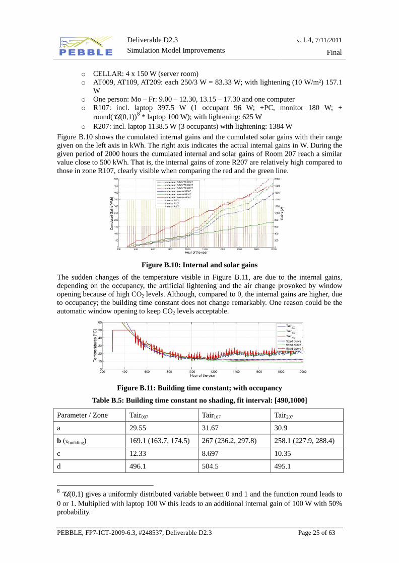
Deliverable D2.3 Simulation Model Improvements
v. 1.4, 7/11/2011
Final
PEBBLE, FP7-ICT-2009-6.3, #248537, Deliverable D2.3 Page 25 of 63
o CELLAR: 4 x 150 W (server room) o AT009, AT109, AT209: each 250/3 W = 83.33 W; with lightening (10 W/m²) 157.1
W o One person: Mo – Fr: 9.00 – 12.30, 13.15 – 17.30 and one computer o R107: incl. laptop 397.5 W (1 occupant 96 W; +PC, monitor 180 W; +
round(U(0,1))8 * laptop 100 W); with lightening: 625 W o R207: incl. laptop 1138.5 W (3 occupants) with lightening: 1384 W
Figure B.10 shows the cumulated internal gains and the cumulated solar gains with their range given on the left axis in kWh. The right axis indicates the actual internal gains in W. During the given period of 2000 hours the cumulated internal and solar gains of Room 207 reach a similar value close to 500 kWh. That is, the internal gains of zone R207 are relatively high compared to those in zone R107, clearly visible when comparing the red and the green line.
Figure B.10: Internal and solar gains
The sudden changes of the temperature visible in Figure B.11, are due to the internal gains, depending on the occupancy, the artificial lightening and the air change provoked by window opening because of high CO2 levels. Although, compared to 0, the internal gains are higher, due to occupancy; the building time constant does not change remarkably. One reason could be the automatic window opening to keep CO2 levels acceptable.
Figure B.11: Building time constant; with occupancy
Table B.5: Building time constant no shading, fit interval: [490,1000]
Parameter / Zone Tair007 Tair107 Tair207
a 29.55 31.67 30.9
b (τbuilding) 169.1 (163.7, 174.5) 267 (236.2, 297.8) 258.1 (227.9, 288.4)
c 12.33 8.697 10.35
d 496.1 504.5 495.1
8 U(0,1) gives a uniformly distributed variable between 0 and 1 and the function round leads to 0 or 1. Multiplied with laptop 100 W this leads to an additional internal gain of 100 W with 50% probability.
Deliverable D2.3 Simulation Model Improvements
v. 1.4, 7/11/2011
Final
PEBBLE, FP7-ICT-2009-6.3, #248537, Deliverable D2.3 Page 26 of 63
C RWTH Building Simulation
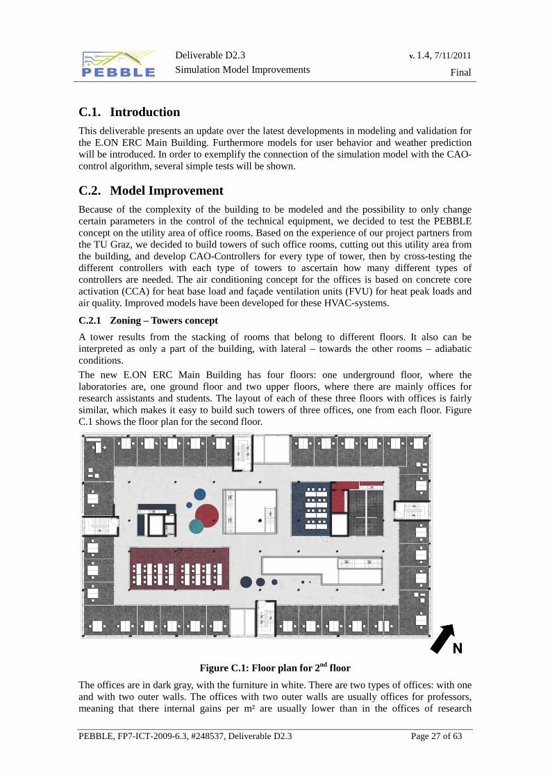
Deliverable D2.3 Simulation Model Improvements
v. 1.4, 7/11/2011
Final
PEBBLE, FP7-ICT-2009-6.3, #248537, Deliverable D2.3 Page 27 of 63
C.1. Introduction This deliverable presents an update over the latest developments in modeling and validation for the E.ON ERC Main Building. Furthermore models for user behavior and weather prediction will be introduced. In order to exemplify the connection of the simulation model with the CAO- control algorithm, several simple tests will be shown.
C.2. Model Improvement Because of the complexity of the building to be modeled and the possibility to only change certain parameters in the control of the technical equipment, we decided to test the PEBBLE concept on the utility area of office rooms. Based on the experience of our project partners from the TU Graz, we decided to build towers of such office rooms, cutting out this utility area from the building, and develop CAO-Controllers for every type of tower, then by cross-testing the different controllers with each type of towers to ascertain how many different types of controllers are needed. The air conditioning concept for the offices is based on concrete core activation (CCA) for heat base load and façade ventilation units (FVU) for heat peak loads and air quality. Improved models have been developed for these HVAC-systems.
C.2.1 Zoning – Towers concept A tower results from the stacking of rooms that belong to different floors. It also can be interpreted as only a part of the building, with lateral – towards the other rooms – adiabatic conditions. The new E.ON ERC Main Building has four floors: one underground floor, where the laboratories are, one ground floor and two upper floors, where there are mainly offices for research assistants and students. The layout of each of these three floors with offices is fairly similar, which makes it easy to build such towers of three offices, one from each floor. Figure C.1 shows the floor plan for the second floor.
Figure C.1: Floor plan for 2nd floor
The offices are in dark gray, with the furniture in white. There are two types of offices: with one and with two outer walls. The offices with two outer walls are usually offices for professors, meaning that there internal gains per m² are usually lower than in the offices of research
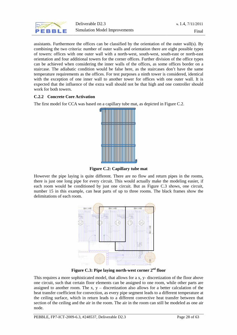
Deliverable D2.3 Simulation Model Improvements
v. 1.4, 7/11/2011
Final
PEBBLE, FP7-ICT-2009-6.3, #248537, Deliverable D2.3 Page 28 of 63
assistants. Furthermore the offices can be classified by the orientation of the outer wall(s). By combining the two criteria: number of outer walls and orientation there are eight possible types of towers: offices with one outer wall with a north-west, south-west, south-east or north-east orientation and four additional towers for the corner offices. Further division of the office types can be achieved when considering the inner walls of the offices, as some offices border on a staircase. The adiabatic condition would be false here, as the staircases don’t have the same temperature requirements as the offices. For test purposes a ninth tower is considered, identical with the exception of one inner wall to another tower for offices with one outer wall. It is expected that the influence of the extra wall should not be that high and one controller should work for both towers.
C.2.2 Concrete Core Activation The first model for CCA was based on a capillary tube mat, as depicted in Figure C.2.
Figure C.2: Capillary tube mat
However the pipe laying is quite different. There are no flow and return pipes in the rooms, there is just one long pipe for every circuit. This would actually make the modeling easier, if each room would be conditioned by just one circuit. But as Figure C.3 shows, one circuit, number 15 in this example, can heat parts of up to three rooms. The black frames show the delimitations of each room.
Figure C.3: Pipe laying north-west corner 2nd floor
This requires a more sophisticated model, that allows for a x, y- discretization of the floor above one circuit, such that certain floor elements can be assigned to one room, while other parts are assigned to another room. The x, y – discretization also allows for a better calculation of the heat transfer coefficient for convection, as every pipe segment leads to a different temperature at the ceiling surface, which in return leads to a different convective heat transfer between that section of the ceiling and the air in the room. The air in the room can still be modeled as one air node.
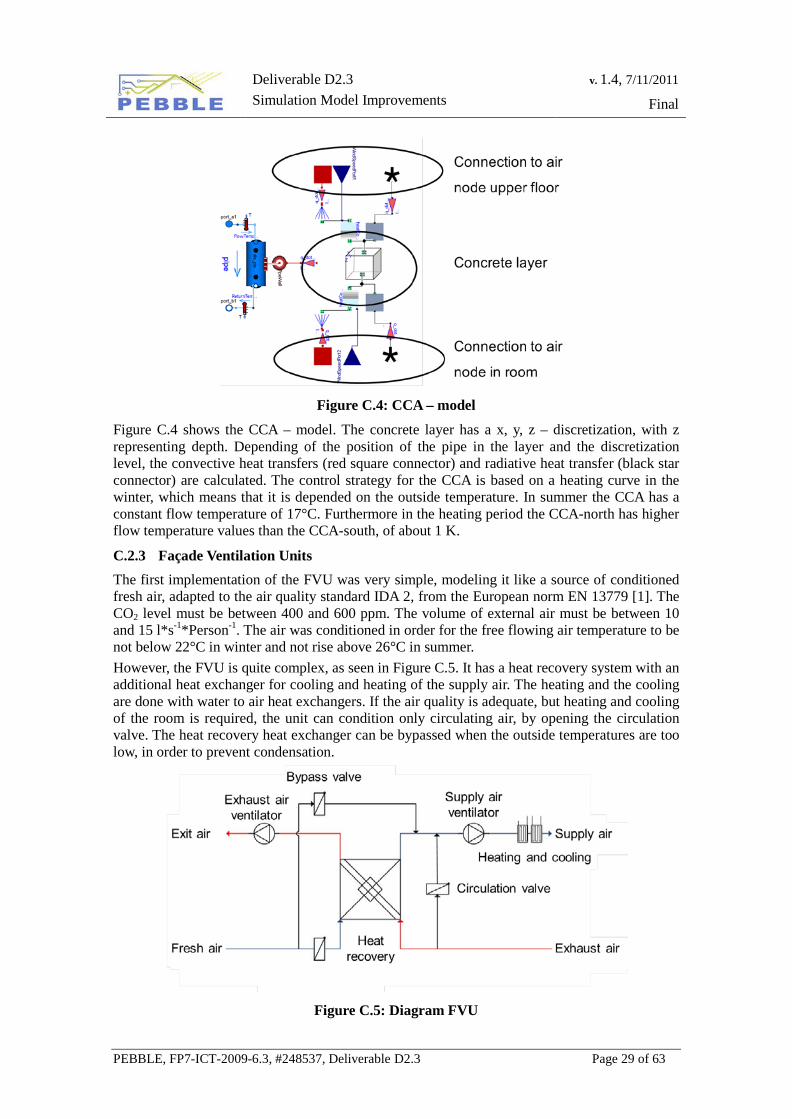
Deliverable D2.3 Simulation Model Improvements
v. 1.4, 7/11/2011
Final
PEBBLE, FP7-ICT-2009-6.3, #248537, Deliverable D2.3 Page 29 of 63
Figure C.4: CCA – model
Figure C.4 shows the CCA – model. The concrete layer has a x, y, z – discretization, with z representing depth. Depending of the position of the pipe in the layer and the discretization level, the convective heat transfers (red square connector) and radiative heat transfer (black star connector) are calculated. The control strategy for the CCA is based on a heating curve in the winter, which means that it is depended on the outside temperature. In summer the CCA has a constant flow temperature of 17°C. Furthermore in the heating period the CCA-north has higher flow temperature values than the CCA-south, of about 1 K.
C.2.3 Façade Ventilation Units The first implementation of the FVU was very simple, modeling it like a source of conditioned fresh air, adapted to the air quality standard IDA 2, from the European norm EN 13779 [1]. The CO2 level must be between 400 and 600 ppm. The volume of external air must be between 10 and 15 l*s-1*Person-1. The air was conditioned in order for the free flowing air temperature to be not below 22°C in winter and not rise above 26°C in summer. However, the FVU is quite complex, as seen in Figure C.5. It has a heat recovery system with an additional heat exchanger for cooling and heating of the supply air. The heating and the cooling are done with water to air heat exchangers. If the air quality is adequate, but heating and cooling of the room is required, the unit can condition only circulating air, by opening the circulation valve. The heat recovery heat exchanger can be bypassed when the outside temperatures are too low, in order to prevent condensation.
Figure C.5: Diagram FVU
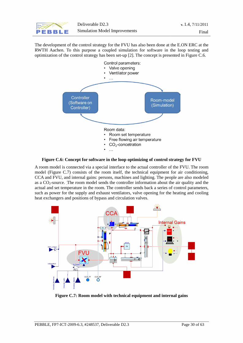
Deliverable D2.3 Simulation Model Improvements
v. 1.4, 7/11/2011
Final
PEBBLE, FP7-ICT-2009-6.3, #248537, Deliverable D2.3 Page 30 of 63
The development of the control strategy for the FVU has also been done at the E.ON ERC at the RWTH Aachen. To this purpose a coupled simulation for software in the loop testing and optimization of the control strategy has been set-up [2]. The concept is presented in Figure C.6.
Figure C.6: Concept for software in the loop optimizing of control strategy for FVU
A room model is connected via a special interface to the actual controller of the FVU. The room model (Figure C.7) consists of the room itself, the technical equipment for air conditioning, CCA and FVU, and internal gains: persons, machines and lighting. The people are also modeled as a CO2-source. .The room model sends the controller information about the air quality and the actual and set temperature in the room. The controller sends back a series of control parameters, such as power for the supply and exhaust ventilators, valve opening for the heating and cooling heat exchangers and positions of bypass and circulation valves.
Figure C.7: Room model with technical equipment and internal gains
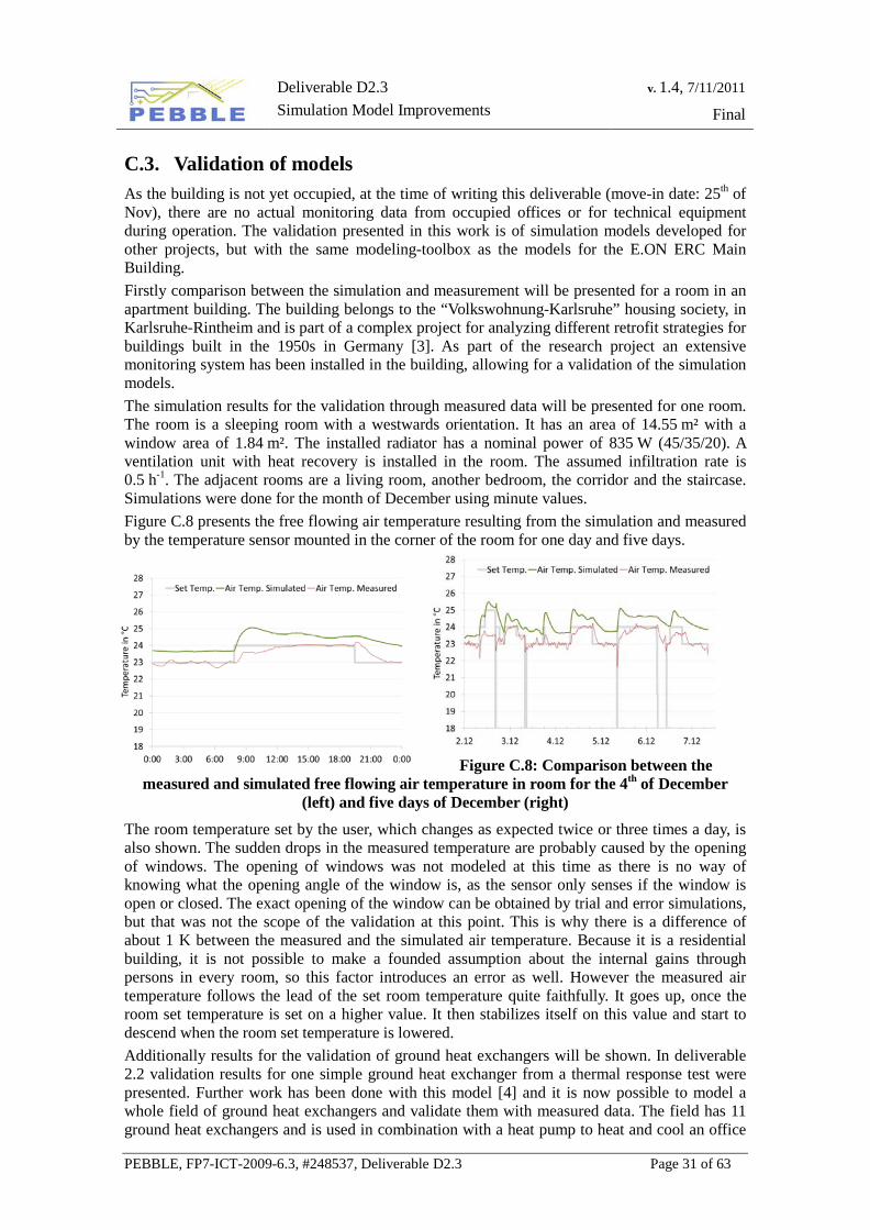
Deliverable D2.3 Simulation Model Improvements
v. 1.4, 7/11/2011
Final
PEBBLE, FP7-ICT-2009-6.3, #248537, Deliverable D2.3 Page 31 of 63
C.3. Validation of models As the building is not yet occupied, at the time of writing this deliverable (move-in date: 25th of Nov), there are no actual monitoring data from occupied offices or for technical equipment during operation. The validation presented in this work is of simulation models developed for other projects, but with the same modeling-toolbox as the models for the E.ON ERC Main Building. Firstly comparison between the simulation and measurement will be presented for a room in an apartment building. The building belongs to the “Volkswohnung-Karlsruhe” housing society, in Karlsruhe-Rintheim and is part of a complex project for analyzing different retrofit strategies for buildings built in the 1950s in Germany [3]. As part of the research project an extensive monitoring system has been installed in the building, allowing for a validation of the simulation models. The simulation results for the validation through measured data will be presented for one room. The room is a sleeping room with a westwards orientation. It has an area of 14.55 m² with a window area of 1.84 m². The installed radiator has a nominal power of 835 W (45/35/20). A ventilation unit with heat recovery is installed in the room. The assumed infiltration rate is 0.5 h-1. The adjacent rooms are a living room, another bedroom, the corridor and the staircase. Simulations were done for the month of December using minute values. Figure C.8 presents the free flowing air temperature resulting from the simulation and measured by the temperature sensor mounted in the corner of the room for one day and five days.
Figure C.8: Comparison between the
measured and simulated free flowing air temperature in room for the 4th of December (left) and five days of December (right)
The room temperature set by the user, which changes as expected twice or three times a day, is also shown. The sudden drops in the measured temperature are probably caused by the opening of windows. The opening of windows was not modeled at this time as there is no way of knowing what the opening angle of the window is, as the sensor only senses if the window is open or closed. The exact opening of the window can be obtained by trial and error simulations, but that was not the scope of the validation at this point. This is why there is a difference of about 1 K between the measured and the simulated air temperature. Because it is a residential building, it is not possible to make a founded assumption about the internal gains through persons in every room, so this factor introduces an error as well. However the measured air temperature follows the lead of the set room temperature quite faithfully. It goes up, once the room set temperature is set on a higher value. It then stabilizes itself on this value and start to descend when the room set temperature is lowered. Additionally results for the validation of ground heat exchangers will be shown. In deliverable 2.2 validation results for one simple ground heat exchanger from a thermal response test were presented. Further work has been done with this model [4] and it is now possible to model a whole field of ground heat exchangers and validate them with measured data. The field has 11 ground heat exchangers and is used in combination with a heat pump to heat and cool an office
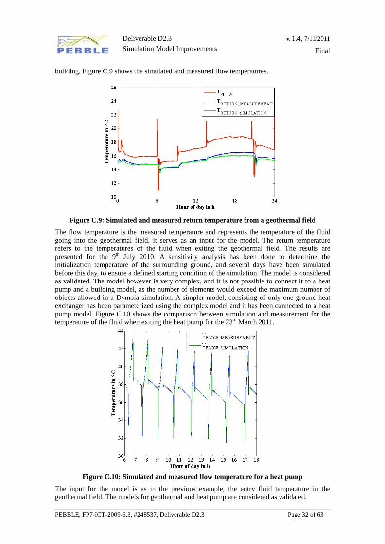
Deliverable D2.3 Simulation Model Improvements
v. 1.4, 7/11/2011
Final
PEBBLE, FP7-ICT-2009-6.3, #248537, Deliverable D2.3 Page 32 of 63
building. Figure C.9 shows the simulated and measured flow temperatures.
Figure C.9: Simulated and measured return temperature from a geothermal field
The flow temperature is the measured temperature and represents the temperature of the fluid going into the geothermal field. It serves as an input for the model. The return temperature refers to the temperatures of the fluid when exiting the geothermal field. The results are presented for the 9th July 2010. A sensitivity analysis has been done to determine the initialization temperature of the surrounding ground, and several days have been simulated before this day, to ensure a defined starting condition of the simulation. The model is considered as validated. The model however is very complex, and it is not possible to connect it to a heat pump and a building model, as the number of elements would exceed the maximum number of objects allowed in a Dymola simulation. A simpler model, consisting of only one ground heat exchanger has been parameterized using the complex model and it has been connected to a heat pump model. Figure C.10 shows the comparison between simulation and measurement for the temperature of the fluid when exiting the heat pump for the 23rd March 2011.
Figure C.10: Simulated and measured flow temperature for a heat pump
The input for the model is as in the previous example, the entry fluid temperature in the geothermal field. The models for geothermal and heat pump are considered as validated.
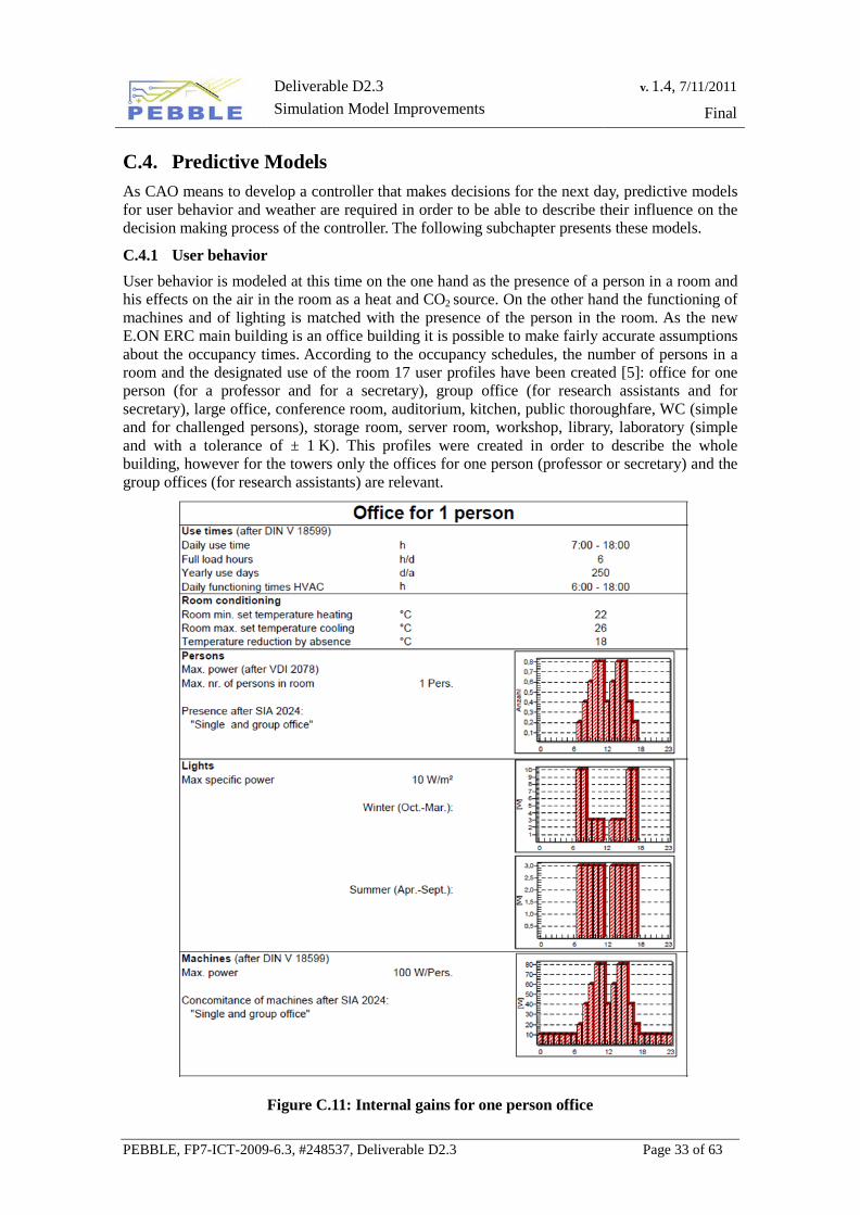
Deliverable D2.3 Simulation Model Improvements
v. 1.4, 7/11/2011
Final
PEBBLE, FP7-ICT-2009-6.3, #248537, Deliverable D2.3 Page 33 of 63
C.4. Predictive Models As CAO means to develop a controller that makes decisions for the next day, predictive models for user behavior and weather are required in order to be able to describe their influence on the decision making process of the controller. The following subchapter presents these models.
C.4.1 User behavior User behavior is modeled at this time on the one hand as the presence of a person in a room and his effects on the air in the room as a heat and CO2 source. On the other hand the functioning of machines and of lighting is matched with the presence of the person in the room. As the new E.ON ERC main building is an office building it is possible to make fairly accurate assumptions about the occupancy times. According to the occupancy schedules, the number of persons in a room and the designated use of the room 17 user profiles have been created [5]: office for one person (for a professor and for a secretary), group office (for research assistants and for secretary), large office, conference room, auditorium, kitchen, public thoroughfare, WC (simple and for challenged persons), storage room, server room, workshop, library, laboratory (simple and with a tolerance of ± 1 K). This profiles were created in order to describe the whole building, however for the towers only the offices for one person (professor or secretary) and the group offices (for research assistants) are relevant.
Figure C.11: Internal gains for one person office
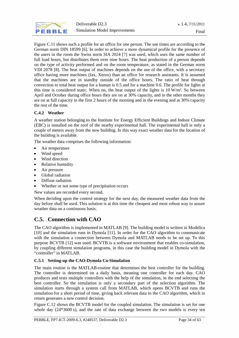
Deliverable D2.3 Simulation Model Improvements
v. 1.4, 7/11/2011
Final
PEBBLE, FP7-ICT-2009-6.3, #248537, Deliverable D2.3 Page 34 of 63
Figure C.11 shows such a profile for an office for one person. The use times are according to the German norm DIN 18599 [6]. In order to achieve a more dynamical profile for the presence of the users in the room the Swiss norm SIA 2024 [7] was used, which uses the same number of full load hours, but distributes them over nine hours. The heat production of a person depends on the type of activity performed and on the room temperature, as stated in the German norm VDI 2078 [8]. The heat output of machines depends on the use of the office, with a secretary office having more machines (fax, Xerox) than an office for research assistants. It is assumed that the machines are in standby outside of the office hours. The ratio of heat through convection to total heat output for a human is 0.5 and for a machine 0.6. The profile for lights at this time is considered static. When on, the heat output of the lights is 10 W/m². So between April and October during office hours they are on at 30% capacity, and in the other months they are on at full capacity in the first 2 hours of the morning and in the evening and at 30% capacity the rest of the time.
C.4.2 Weather A weather station belonging to the Institute for Energy Efficient Buildings and Indoor Climate (EBC) is installed on the roof of the nearby experimental hall. The experimental hall is only a couple of meters away from the new building. In this way exact weather data for the location of the building is available. The weather data comprises the following information: • Air temperature • Wind speed • Wind direction • Relative humidity • Air pressure • Global radiation • Diffuse radiation • Whether or not some type of precipitation occurs New values are recorded every second. When deciding upon the control strategy for the next day, the measured weather data from the day before shall be used. This solution is at this time the cheapest and most robust way to assure weather data on a continuous basis.
C.5. Connection with CAO The CAO algorithm is implemented in MATLAB [9]. The building model is written in Modelica [10] and the simulation runs in Dymola [11]. In order for the CAO algorithm to communicate with the simulation a connection between Dymola and MATLAB needs to be set up. To this purpose BCVTB [12] was used. BCVTB is a software environment that enables co-simulation, by coupling different simulation programs, in this case the building model in Dymola with the “controller” in MATLAB.
C.5.1 Setting-up the CAO-Dymola Co-Simulation The main routine is the MATLAB-routine that determines the best controller for the building. The controller is determined on a daily basis, meaning one controller for each day. CAO produces and tests multiple controllers with the help of the simulation, in the end selecting the best controller. So the simulation is only a secondary part of the selection algorithm. The simulation starts through a system call from MATLAB, which opens BCVTB and runs the simulation for a short period of time, giving back relevant data to the CAO algorithm, which in return generates a new control decision. Figure C.12 shows the BCVTB model for the coupled simulation. The simulation is set for one whole day (24*3600 s), and the rate of data exchange between the two models is every ten
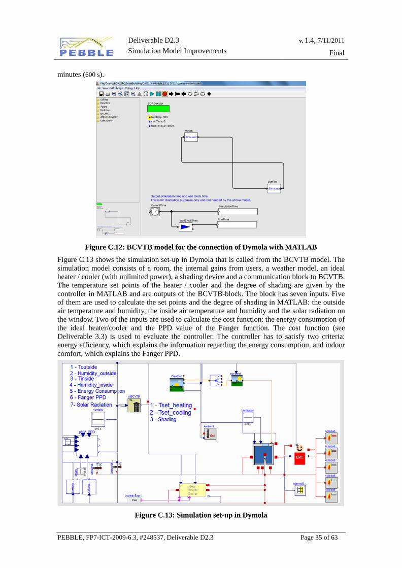
Deliverable D2.3 Simulation Model Improvements
v. 1.4, 7/11/2011
Final
PEBBLE, FP7-ICT-2009-6.3, #248537, Deliverable D2.3 Page 35 of 63
minutes (600 s).
Figure C.12: BCVTB model for the connection of Dymola with MATLAB
Figure C.13 shows the simulation set-up in Dymola that is called from the BCVTB model. The simulation model consists of a room, the internal gains from users, a weather model, an ideal heater / cooler (with unlimited power), a shading device and a communication block to BCVTB. The temperature set points of the heater / cooler and the degree of shading are given by the controller in MATLAB and are outputs of the BCVTB-block. The block has seven inputs. Five of them are used to calculate the set points and the degree of shading in MATLAB: the outside air temperature and humidity, the inside air temperature and humidity and the solar radiation on the window. Two of the inputs are used to calculate the cost function: the energy consumption of the ideal heater/cooler and the PPD value of the Fanger function. The cost function (see Deliverable 3.3) is used to evaluate the controller. The controller has to satisfy two criteria: energy efficiency, which explains the information regarding the energy consumption, and indoor comfort, which explains the Fanger PPD.
Figure C.13: Simulation set-up in Dymola
Deliverable D2.3 Simulation Model Improvements
v. 1.4, 7/11/2011
Final
PEBBLE, FP7-ICT-2009-6.3, #248537, Deliverable D2.3 Page 36 of 63
C.6. Conclusion, Summary and Outlook The goal of this deliverable was to show the developments of the thermal simulation models since Deliverable 2.2. The models have been extended to include more exact models for the FVU and the CCA. Also the decision has been made to only focus on office spaces and group them in towers of three offices, each with a different orientation. Validation work for the model components was done with data from other research projects, as the building has only been occupied since the end of November. The employed predictive models for user behavior and weather have been presented. The basics of connecting the Dymola simulation with the CAO algorithm were highlighted. Further details about the CAO connection to the Dymola model and exemplary results can be found in D3.3. As a next step the model should be validated as soon as data from the monitoring system is available. In parallel controllers for the different types of towers will be developed and compared to one another in order to obtain the optimal number of different controllers.
Deliverable D2.3 Simulation Model Improvements
v. 1.4, 7/11/2011
Final
PEBBLE, FP7-ICT-2009-6.3, #248537, Deliverable D2.3 Page 37 of 63
C.7. References [1] DIN EN 13779, Ventilation for non-residential buildings – Performance requirements for
ventilation and room-conditioning systems, Beuth Verlag, 2007. [2] Huber, M., Constantin, A., Müller, D., Optimierung der Regelungsstrategie für ein
Fassadenlüftungsgerät mit Hilfe von Simulation, DKV-Tagung, Aachen 2011 [3] Calì, D., Osterhage, T. and Mueller, D., Field study of retrofit solutions for residential
housing, E.ON Energy Research Center, RWTH Aachen University, 2010 [4] Comanns, T., Modellierung und Simulation eines LowEx-Gebäudes in der
objektorinetierten Programmiersprache Modelica, student thesis, E.ON Energy Research Center, RWTH Aachen University, 2011
[5] Chivite, A., Energetische Bilanzierung der E.ON ERC Hauptgebäude, student thesis, E.ON Energy Research Center, RWTH Aachen University, 2011
[6] DIN 18599, Energy efficiency of buildings – Calculation of the net, final and primary energy demand for heating, cooling, ventilation, domestic hot water and lighting, part 1, Beuth Verlag, 2007
[7] SIA 2024, Standard-Nutzungsbedingungen für Energie- und Gebäudetechnik, Verlag SIA 2006
[8] VDI 2078, Cooling Load Calculation of Air-conditioned Rooms (VDI Cooling Load Regulations), Beuth Verlag, 1996
[9] MATLAB, Version 2010b, MathWorks, 2010 [10] Modelica, Version 3.2, Modelica Association, 2010. [11] Dymola, Version 7.4, Dynamic Modeling Laboratory, Dassault Systems AB, 2010. [12] BCVTB, Building Controls Virtual Test Bed, Laurence Berkley National Laboratory, 2011
Deliverable D2.3 Simulation Model Improvements
v. 1.4, 7/11/2011
Final
PEBBLE, FP7-ICT-2009-6.3, #248537, Deliverable D2.3 Page 38 of 63
D TUC Building Simulation
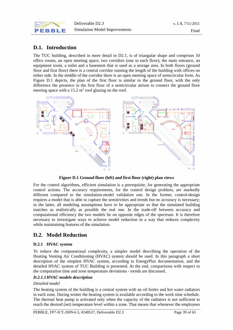
Deliverable D2.3 Simulation Model Improvements
v. 1.4, 7/11/2011
Final
PEBBLE, FP7-ICT-2009-6.3, #248537, Deliverable D2.3 Page 39 of 63
D.1. Introduction The TUC building, described in more detail in D2.1, is of triangular shape and comprises 10 office rooms, an open meeting space, two corridors (one in each floor), the main entrance, an equipment room, a toilet and a basement that is used as a storage area. In both floors (ground floor and first floor) there is a central corridor running the length of the building with offices on either side. In the middle of the corridor there is an open meeting space of semicircular form. As Figure D.1 depicts, the plan of the first floor is similar to the ground floor, with the only difference the presence in the first floor of a semicircular atrium to connect the ground floor meeting space with a 15.2 m2 roof glazing on the roof.
Figure D.1 Ground floor (left) and first floor (right) plan views
For the control algorithms, efficient simulation is a prerequisite, for generating the appropriate control actions. The accuracy requirements, for the control design problem, are markedly different compared to the simulation-model validation one. In the former, control-design requires a model that is able to capture the sensitivities and trends but no accuracy is necessary; in the latter, all modeling assumptions have to be appropriate so that the simulated building matches as realistically as possible the real one. In the trade-off between accuracy and computational efficiency the two models lie on opposite edges of the spectrum. It is therefore necessary to investigate ways to achieve model reduction in a way that reduces complexity while maintaining features of the simulation.
D.2. Model Reduction D.2.1 HVAC system To reduce the computational complexity, a simpler model describing the operation of the Heating Venting Air Conditioning (HVAC) system should be used. In this paragraph a short description of the simplest HVAC system, according to EnergyPlus documentation, and the detailed HVAC system of TUC Building is presented. At the end, comparisons with respect to the computation time and zone temperature deviations - trends are discussed. D.2.1.1 HVAC models description Detailed model The heating system of the building is a central system with an oil boiler and hot water radiators in each zone. During winter the heating system is available according to the work time schedule. The thermal heat pump is activated only when the capacity of the radiators is not sufficient to reach the desired (set) temperature level within a zone. That means that whenever the employees
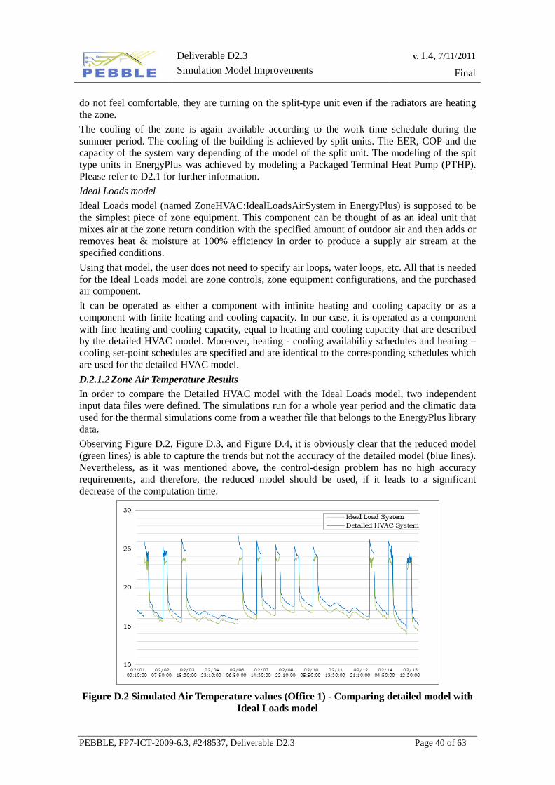
Deliverable D2.3 Simulation Model Improvements
v. 1.4, 7/11/2011
Final
PEBBLE, FP7-ICT-2009-6.3, #248537, Deliverable D2.3 Page 40 of 63
do not feel comfortable, they are turning on the split-type unit even if the radiators are heating the zone. The cooling of the zone is again available according to the work time schedule during the summer period. The cooling of the building is achieved by split units. The EER, COP and the capacity of the system vary depending of the model of the split unit. The modeling of the spit type units in EnergyPlus was achieved by modeling a Packaged Terminal Heat Pump (PTHP). Please refer to D2.1 for further information. Ideal Loads model Ideal Loads model (named ZoneHVAC:IdealLoadsAirSystem in EnergyPlus) is supposed to be the simplest piece of zone equipment. This component can be thought of as an ideal unit that mixes air at the zone return condition with the specified amount of outdoor air and then adds or removes heat & moisture at 100% efficiency in order to produce a supply air stream at the specified conditions. Using that model, the user does not need to specify air loops, water loops, etc. All that is needed for the Ideal Loads model are zone controls, zone equipment configurations, and the purchased air component. It can be operated as either a component with infinite heating and cooling capacity or as a component with finite heating and cooling capacity. In our case, it is operated as a component with fine heating and cooling capacity, equal to heating and cooling capacity that are described by the detailed HVAC model. Moreover, heating - cooling availability schedules and heating – cooling set-point schedules are specified and are identical to the corresponding schedules which are used for the detailed HVAC model. D.2.1.2 Zone Air Temperature Results In order to compare the Detailed HVAC model with the Ideal Loads model, two independent input data files were defined. The simulations run for a whole year period and the climatic data used for the thermal simulations come from a weather file that belongs to the EnergyPlus library data. Observing Figure D.2, Figure D.3, and Figure D.4, it is obviously clear that the reduced model (green lines) is able to capture the trends but not the accuracy of the detailed model (blue lines). Nevertheless, as it was mentioned above, the control-design problem has no high accuracy requirements, and therefore, the reduced model should be used, if it leads to a significant decrease of the computation time.
Figure D.2 Simulated Air Temperature values (Office 1) - Comparing detailed model with
Ideal Loads model
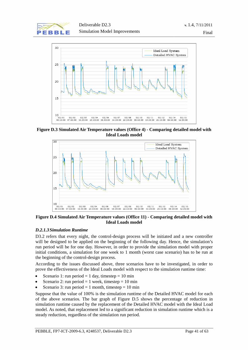
Deliverable D2.3 Simulation Model Improvements
v. 1.4, 7/11/2011
Final
PEBBLE, FP7-ICT-2009-6.3, #248537, Deliverable D2.3 Page 41 of 63
Figure D.3 Simulated Air Temperature values (Office 4) - Comparing detailed model with
Ideal Loads model
Figure D.4 Simulated Air Temperature values (Office 11) - Comparing detailed model with
Ideal Loads model
D.2.1.3 Simulation Runtime D3.2 refers that every night, the control-design process will be initiated and a new controller will be designed to be applied on the beginning of the following day. Hence, the simulation’s run period will be for one day. However, in order to provide the simulation model with proper initial conditions, a simulation for one week to 1 month (worst case scenario) has to be run at the beginning of the control-design process. According to the issues discussed above, three scenarios have to be investigated, in order to prove the effectiveness of the Ideal Loads model with respect to the simulation runtime time: • Scenario 1: run period = 1 day, timestep = 10 min • Scenario 2: run period = 1 week, timestep = 10 min • Scenario 3: run period = 1 month, timestep = 10 min Suppose that the value of 100% is the simulation runtime of the Detailed HVAC model for each of the above scenarios. The bar graph of Figure D.5 shows the percentage of reduction in simulation runtime caused by the replacement of the Detailed HVAC model with the Ideal Load model. As noted, that replacement led to a significant reduction in simulation runtime which is a steady reduction, regardless of the simulation run period.
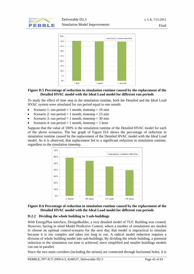
Deliverable D2.3 Simulation Model Improvements
v. 1.4, 7/11/2011
Final
PEBBLE, FP7-ICT-2009-6.3, #248537, Deliverable D2.3 Page 42 of 63
Figure D.5 Percentage of reduction in simulation runtime caused by the replacement of the
Detailed HVAC model with the Ideal Load model for different run periods
To study the effect of time step in the simulation runtime, both the Detailed and the Ideal Load HVAC system were simulated for run period equal to one month: • Scenario 1: run period = 1 month, timestep = 10 min • Scenario 2: run period = 1 month, timestep = 15 min • Scenario 3: run period = 1 month, timestep = 30 min • Scenario 4: run period = 1 month, timestep = 1 hour Suppose that the value of 100% is the simulation runtime of the Detailed HVAC model for each of the above scenarios. The bar graph of Figure D.6 shows the percentage of reduction in simulation runtime caused by the replacement of the Detailed HVAC model with the Ideal Load model. As it is observed, that replacement led to a significant reduction in simulation runtime, regardless to the simulation timestep.
Figure D.6 Percentage of reduction in simulation runtime caused by the replacement of the
Detailed HVAC model with the Ideal Load model for different run periods
D.2.2 Dividing the whole building to 3 sub-buildings With EnergyPlus interface, DesignBuilder, a very detailed model of TUC Building was created. However, having in mind Model Predictive Control, where a number of simulations are needed to choose an optimal control-scenario for the next day, that model is impractical to simulate because it is too complex and takes too long to run. A radical model reduction requires a division of whole building model into sub-buildings. By dividing the whole building, a potential reduction to the simulation run time is achieved, since simplified and smaller buildings models can run in parallel. Since the two main corridors (including the atrium) are connected through horizontal holes, it is
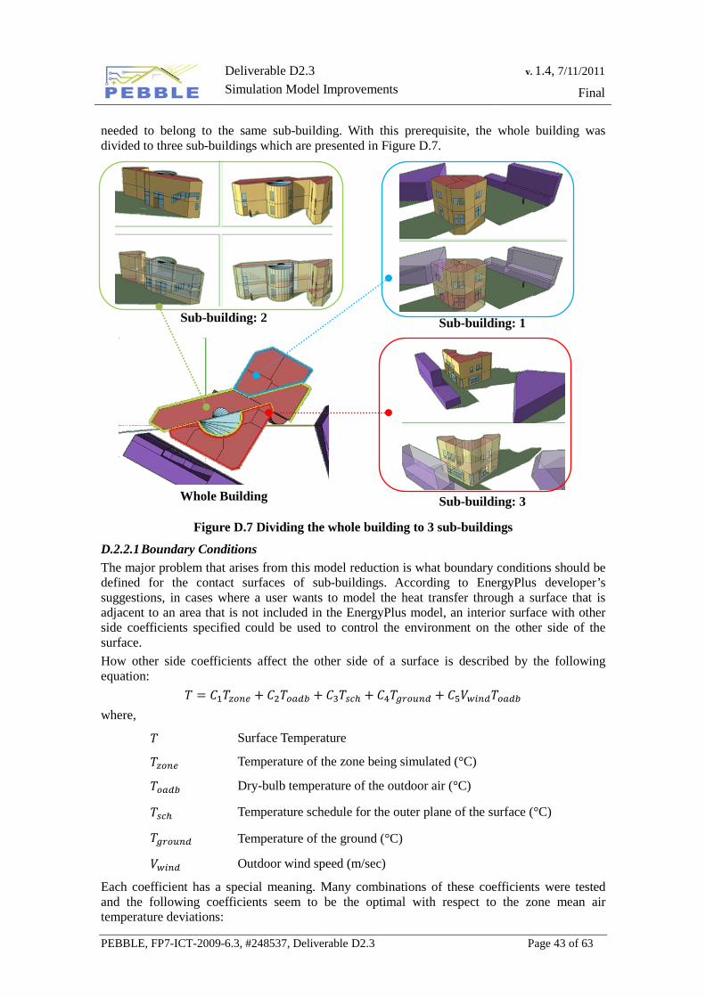
Deliverable D2.3 Simulation Model Improvements
v. 1.4, 7/11/2011
Final
PEBBLE, FP7-ICT-2009-6.3, #248537, Deliverable D2.3 Page 43 of 63
needed to belong to the same sub-building. With this prerequisite, the whole building was divided to three sub-buildings which are presented in Figure D.7.
Sub-building: 2
Sub-building: 1
Whole Building
Sub-building: 3
Figure D.7 Dividing the whole building to 3 sub-buildings
D.2.2.1 Boundary Conditions The major problem that arises from this model reduction is what boundary conditions should be defined for the contact surfaces of sub-buildings. According to EnergyPlus developer’s suggestions, in cases where a user wants to model the heat transfer through a surface that is adjacent to an area that is not included in the EnergyPlus model, an interior surface with other side coefficients specified could be used to control the environment on the other side of the surface. How other side coefficients affect the other side of a surface is described by the following equation:
𝑇 = 𝐶1𝑇𝑧𝑜𝑛𝑒 + 𝐶2𝑇𝑜𝑎𝑑𝑏 + 𝐶3𝑇𝑠𝑐ℎ + 𝐶4𝑇𝑔𝑟𝑜𝑢𝑛𝑑 + 𝐶5𝑉𝑤𝑖𝑛𝑑𝑇𝑜𝑎𝑑𝑏 where,
𝑇 Surface Temperature
𝑇𝑧𝑜𝑛𝑒 Temperature of the zone being simulated (°C)
𝑇𝑜𝑎𝑑𝑏 Dry-bulb temperature of the outdoor air (°C)
𝑇𝑠𝑐ℎ Temperature schedule for the outer plane of the surface (°C)
𝑇𝑔𝑟𝑜𝑢𝑛𝑑 Temperature of the ground (°C)
𝑉𝑤𝑖𝑛𝑑 Outdoor wind speed (m/sec)
Each coefficient has a special meaning. Many combinations of these coefficients were tested and the following coefficients seem to be the optimal with respect to the zone mean air temperature deviations:
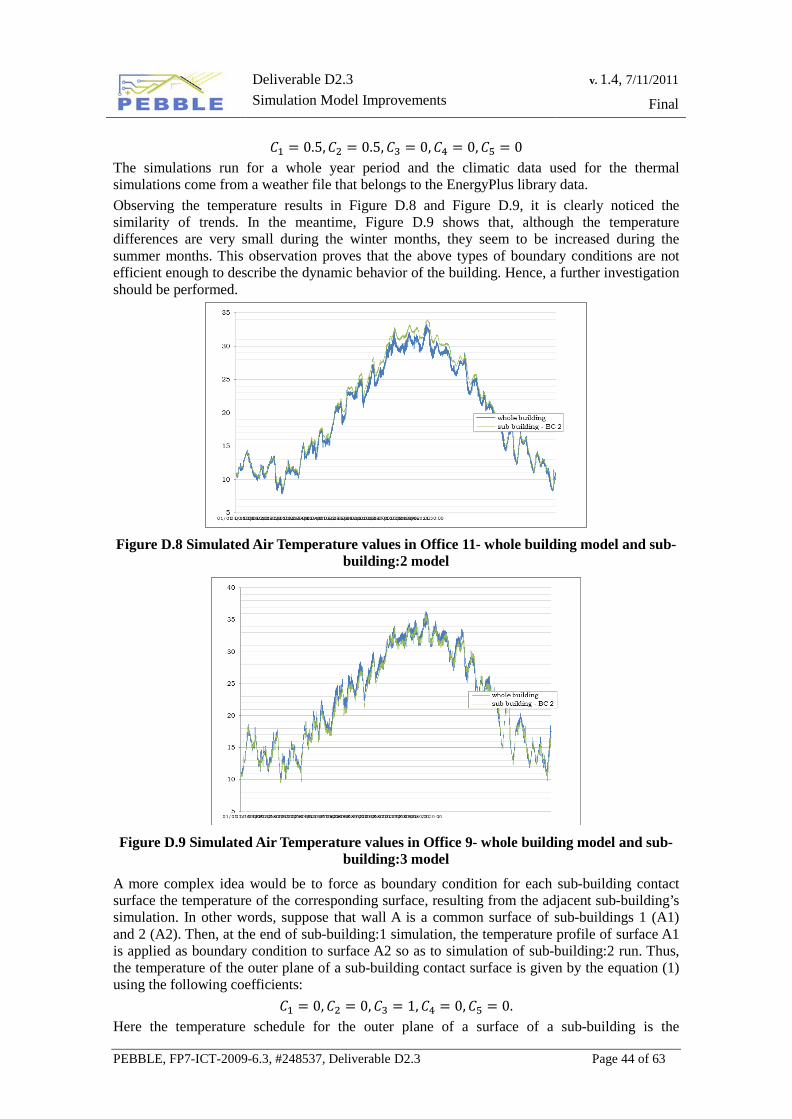
Deliverable D2.3 Simulation Model Improvements
v. 1.4, 7/11/2011
Final
PEBBLE, FP7-ICT-2009-6.3, #248537, Deliverable D2.3 Page 44 of 63
𝐶1 = 0.5,𝐶2 = 0.5,𝐶3 = 0,𝐶4 = 0,𝐶5 = 0 The simulations run for a whole year period and the climatic data used for the thermal simulations come from a weather file that belongs to the EnergyPlus library data. Observing the temperature results in Figure D.8 and Figure D.9, it is clearly noticed the similarity of trends. In the meantime, Figure D.9 shows that, although the temperature differences are very small during the winter months, they seem to be increased during the summer months. This observation proves that the above types of boundary conditions are not efficient enough to describe the dynamic behavior of the building. Hence, a further investigation should be performed.
Figure D.8 Simulated Air Temperature values in Office 11- whole building model and sub-
building:2 model
Figure D.9 Simulated Air Temperature values in Office 9- whole building model and sub-
building:3 model
A more complex idea would be to force as boundary condition for each sub-building contact surface the temperature of the corresponding surface, resulting from the adjacent sub-building’s simulation. In other words, suppose that wall A is a common surface of sub-buildings 1 (A1) and 2 (A2). Then, at the end of sub-building:1 simulation, the temperature profile of surface A1 is applied as boundary condition to surface A2 so as to simulation of sub-building:2 run. Thus, the temperature of the outer plane of a sub-building contact surface is given by the equation (1) using the following coefficients:
𝐶1 = 0,𝐶2 = 0,𝐶3 = 1,𝐶4 = 0,𝐶5 = 0. Here the temperature schedule for the outer plane of a surface of a sub-building is the
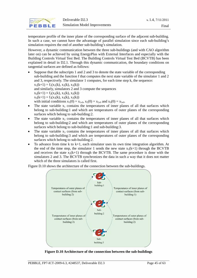
Deliverable D2.3 Simulation Model Improvements
v. 1.4, 7/11/2011
Final
PEBBLE, FP7-ICT-2009-6.3, #248537, Deliverable D2.3 Page 45 of 63
temperature profile of the inner plane of the corresponding surface of the adjacent sub-building. In such a case, we cannot have the advantage of parallel simulation since each sub-building’s simulation requires the end of another sub-building’s simulation. However, a dynamic communication between the three sub-buildings (and with CAO algorithm later on) can be achieved by using EnergyPlus with External Interfaces and especially with the Building Controls Virtual Test Bed. The Building Controls Virtual Test Bed (BCVTB) has been explained in detail in D2.1. Through this dynamic communication, the boundary conditions on tangential surfaces are defined as follows: • Suppose that the subscripts 1 and 2 and 3 to denote the state variable of the corresponding
sub-building and the function f that computes the next state variable of the simulator 1 and 2 and 3, respectively. The simulator 1 computes, for each time step k, the sequence: x1(k+1) = f1(x1(k), x2(k), x3(k)) and similarly, simulators 2 and 3 compute the sequences x2(k+1) = f2(x2(k), x1(k), x2(k)) x3(k+1) = f3(x3(k), x3(k), x2(k)) with initial conditions x1(0) = x1,0, x2(0) = x2,0 and x3(0) = x3,0.
• The state variable x1 contains the temperatures of inner planes of all that surfaces which belong to sub-building:1 and which are temperatures of outer planes of the corresponding surfaces which belong to sub-building:2.
• The state variable x2 contains the temperatures of inner planes of all that surfaces which belong to sub-building:2 and which are temperatures of outer planes of the corresponding surfaces which belong to sub-building:1 and sub-building:3.
• The state variable x3 contains the temperatures of inner planes of all that surfaces which belong to sub-building:3 and which are temperatures of outer planes of the corresponding surfaces which belong to sub-building:2.
• To advance from time k to k+1, each simulator uses its own time integration algorithm. At the end of the time step, the simulator 1 sends the new state x1(k+1) through the BCVTB and receives the state x2(k+1) through the BCVTB. The same procedure is done with the simulators 2 and 3. The BCVTB synchronizes the data in such a way that it does not matter which of the three simulators is called first.
Figure D.10 shows the architecture of the connection between the sub-buildings.
Figure D.10 Architecture of the connection between the sub-buildings
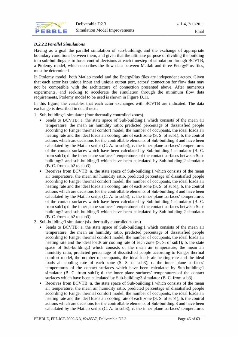
Deliverable D2.3 Simulation Model Improvements
v. 1.4, 7/11/2011
Final
PEBBLE, FP7-ICT-2009-6.3, #248537, Deliverable D2.3 Page 46 of 63
D.2.2.2 Parallel Simulations Having as a goal the parallel simulation of sub-buildings and the exchange of appropriate boundary conditions between them, and given that the ultimate purpose of dividing the building into sub-buildings is to force control decisions at each timestep of simulation through BCVTB, a Ptolemy model, which describes the flow data between Matlab and three EnergyPlus files, must be determined. In Ptolemy model, both Matlab model and the EnergyPlus files are independent actors. Given that each actor has unique input and unique output port, actors’ connection for flow data may not be compatible with the architecture of connection presented above. After numerous experiments, and seeking to accelerate the simulation through the minimum flow data requirements, Ptolemy model to be used is shown in Figure D.11. In this figure, the variables that each actor exchanges with BCVTB are indicated. The data exchange is described in detail next: 1. Sub-building:1 simulator (four thermally controlled zones)
• Sends to BCVTB: a. the state space of Sub-building:1 which consists of the mean air temperature, the mean air humidity ratio, predicted percentage of dissatisfied people according to Fanger thermal comfort model, the number of occupants, the ideal loads air heating rate and the ideal loads air cooling rate of each zone (S. S. of sub1); b. the control actions which are decisions for the controllable elements of Sub-building:3 and have been calculated by the Matlab script (C. A. to sub3); c. the inner plane surfaces’ temperatures of the contact surfaces which have been calculated by Sub-building:1 simulator (B. C. from sub1); d. the inner plane surfaces’ temperatures of the contact surfaces between Sub-building:2 and sub-building:3 which have been calculated by Sub-building:2 simulator (B. C. from sub2 to sub3).
• Receives from BCVTB: a. the state space of Sub-building:1 which consists of the mean air temperature, the mean air humidity ratio, predicted percentage of dissatisfied people according to Fanger thermal comfort model, the number of occupants, the ideal loads air heating rate and the ideal loads air cooling rate of each zone (S. S. of sub1); b. the control actions which are decisions for the controllable elements of Sub-building:3 and have been calculated by the Matlab script (C. A. to sub3); c. the inner plane surfaces’ temperatures of the contact surfaces which have been calculated by Sub-building:1 simulator (B. C. from sub1); d. the inner plane surfaces’ temperatures of the contact surfaces between Sub-building:2 and sub-building:3 which have been calculated by Sub-building:2 simulator (B. C. from sub2 to sub3).
2. Sub-building:3 simulator (six thermally controlled zones) • Sends to BCVTB: a. the state space of Sub-building:1 which consists of the mean air
temperature, the mean air humidity ratio, predicted percentage of dissatisfied people according to Fanger thermal comfort model, the number of occupants, the ideal loads air heating rate and the ideal loads air cooling rate of each zone (S. S. of sub1); b. the state space of Sub-building:3 which consists of the mean air temperature, the mean air humidity ratio, predicted percentage of dissatisfied people according to Fanger thermal comfort model, the number of occupants, the ideal loads air heating rate and the ideal loads air cooling rate of each zone (S. S. of sub3); c. the inner plane surfaces’ temperatures of the contact surfaces which have been calculated by Sub-building:1 simulator (B. C. from sub1); d. the inner plane surfaces’ temperatures of the contact surfaces which have been calculated by Sub-building:3 simulator (B. C. from sub3).
• Receives from BCVTB: a. the state space of Sub-building:1 which consists of the mean air temperature, the mean air humidity ratio, predicted percentage of dissatisfied people according to Fanger thermal comfort model, the number of occupants, the ideal loads air heating rate and the ideal loads air cooling rate of each zone (S. S. of sub1); b. the control actions which are decisions for the controllable elements of Sub-building:3 and have been calculated by the Matlab script (C. A. to sub3); c. the inner plane surfaces’ temperatures
Deliverable D2.3 Simulation Model Improvements
v. 1.4, 7/11/2011
Final
PEBBLE, FP7-ICT-2009-6.3, #248537, Deliverable D2.3 Page 47 of 63
of the contact surfaces which have been calculated by Sub-building:1 simulator (B. C. from sub1); d. the inner plane surfaces’ temperatures of the contact surfaces between Sub-building:2 and sub-building:3 which have been calculated by Sub-building:2 simulator (B. C. from sub2 to sub3).
3. Sub-building:2 simulator • Receives from BCVTB: a. the state space of Sub-building:1 which consists of the mean
air temperature, the mean air humidity ratio, predicted percentage of dissatisfied people according to Fanger thermal comfort model, the number of occupants, the ideal loads air heating rate and the ideal loads air cooling rate of each zone (S. S. of sub1); b. the state space of Sub-building:3 which consists of the mean air temperature, the mean air humidity ratio, predicted percentage of dissatisfied people according to Fanger thermal comfort model, the number of occupants, the ideal loads air heating rate and the ideal loads air cooling rate of each zone (S. S. of sub3); c. the inner plane surfaces’ temperatures of the contact surfaces which have been calculated by Sub-building:1 simulator (B. C. from sub1); d. the inner plane surfaces’ temperatures of the contact surfaces which have been calculated by Sub-building:3 simulator (B. C. from sub3).
• Receives from BCVTB: a. the state space of Sub-building:1 which consists of the mean air temperature, the mean air humidity ratio, predicted percentage of dissatisfied people according to Fanger thermal comfort model, the number of occupants, the ideal loads air heating rate and the ideal loads air cooling rate of each zone (S. S. of sub1); a. the state space of Sub-building:3 which consists of the mean air temperature, the mean air humidity ratio, predicted percentage of dissatisfied people according to Fanger thermal comfort model, the number of occupants, the ideal loads air heating rate and the ideal loads air cooling rate of each zone (S. S. of sub3); c. the inner plane surfaces’ temperatures of the contact surfaces which have been calculated by Sub-building:2 simulator (B. C. from sub2).
4. “Matlab Script: Calculating control actions” simulator • Sends to BCVTB: a. the state space of Sub-building:1 which consists of the mean air
temperature, the mean air humidity ratio, predicted percentage of dissatisfied people according to Fanger thermal comfort model, the number of occupants, the ideal loads air heating rate and the ideal loads air cooling rate of each zone (S. S. of sub1); b. the control actions which are decisions for the controllable elements of Sub-building:3 and have been calculated by the Matlab script (C. A. to sub3); c. the inner plane surfaces’ temperatures of the contact surfaces which have been calculated by Sub-building:2 simulator (B. C. from sub2).
• Receives from BCVTB: a. the state space of Sub-building:1 which consists of the mean air temperature, the mean air humidity ratio, predicted percentage of dissatisfied people according to Fanger thermal comfort model, the number of occupants, the ideal loads air heating rate and the ideal loads air cooling rate of each zone (S. S. of sub1); b. the state space of Sub-building:3 which consists of the mean air temperature, the mean air humidity ratio, predicted percentage of dissatisfied people according to Fanger thermal comfort model, the number of occupants, the ideal loads air heating rate and the ideal loads air cooling rate of each zone (S. S. of sub3); c. the inner plane surfaces’ temperatures of the contact surfaces which have been calculated by Sub-building:1 simulator (B. C. from sub1); d. the inner plane surfaces’ temperatures of the contact surfaces which have been calculated by Sub-building:3 simulator (B. C. from sub3).
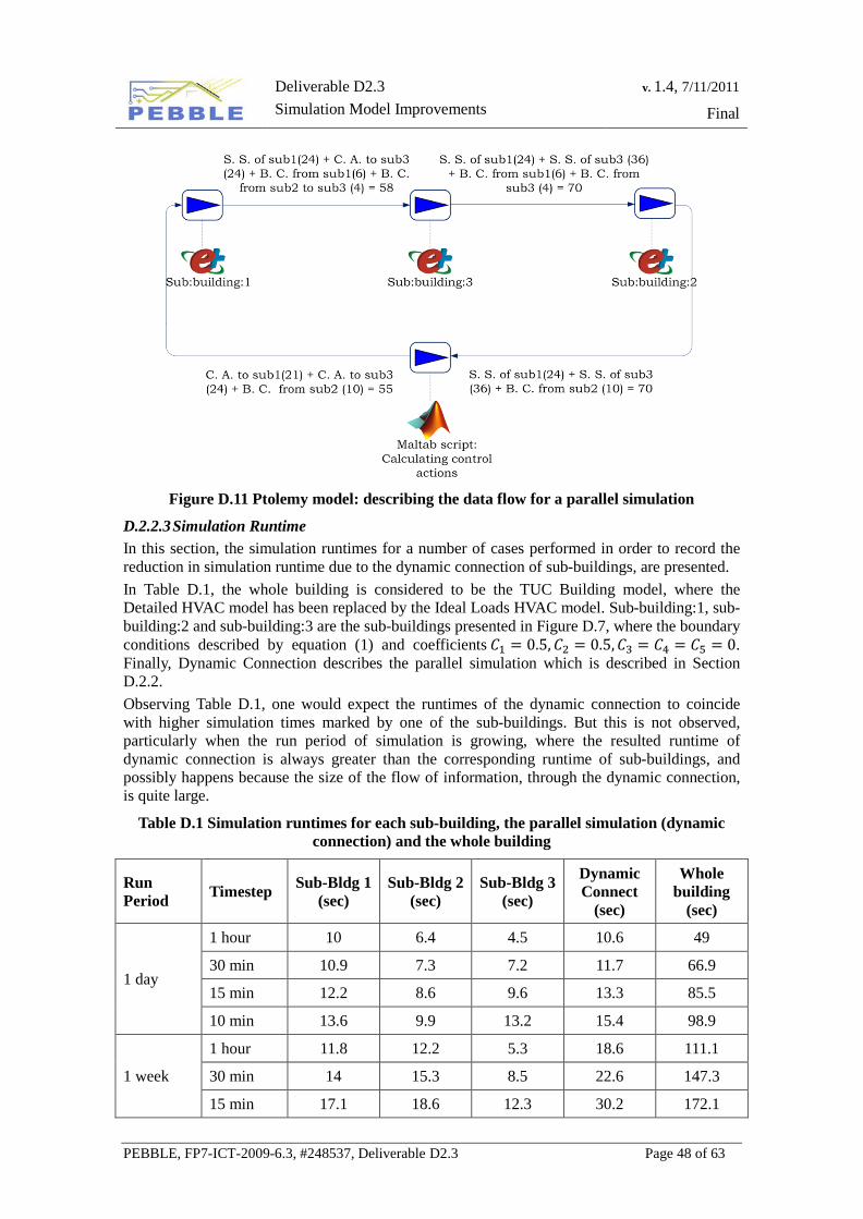
Deliverable D2.3 Simulation Model Improvements
v. 1.4, 7/11/2011
Final
PEBBLE, FP7-ICT-2009-6.3, #248537, Deliverable D2.3 Page 48 of 63
Figure D.11 Ptolemy model: describing the data flow for a parallel simulation
D.2.2.3 Simulation Runtime In this section, the simulation runtimes for a number of cases performed in order to record the reduction in simulation runtime due to the dynamic connection of sub-buildings, are presented. In Table D.1, the whole building is considered to be the TUC Building model, where the Detailed HVAC model has been replaced by the Ideal Loads HVAC model. Sub-building:1, sub-building:2 and sub-building:3 are the sub-buildings presented in Figure D.7, where the boundary conditions described by equation (1) and coefficients 𝐶1 = 0.5,𝐶2 = 0.5,𝐶3 = 𝐶4 = 𝐶5 = 0. Finally, Dynamic Connection describes the parallel simulation which is described in Section D.2.2. Observing Table D.1, one would expect the runtimes of the dynamic connection to coincide with higher simulation times marked by one of the sub-buildings. But this is not observed, particularly when the run period of simulation is growing, where the resulted runtime of dynamic connection is always greater than the corresponding runtime of sub-buildings, and possibly happens because the size of the flow of information, through the dynamic connection, is quite large.
Table D.1 Simulation runtimes for each sub-building, the parallel simulation (dynamic connection) and the whole building
Run Period Timestep Sub-Bldg 1
(sec) Sub-Bldg 2
(sec) Sub-Bldg 3
(sec)
Dynamic Connect
(sec)
Whole building
(sec)
1 day
1 hour 10 6.4 4.5 10.6 49
30 min 10.9 7.3 7.2 11.7 66.9
15 min 12.2 8.6 9.6 13.3 85.5
10 min 13.6 9.9 13.2 15.4 98.9
1 week
1 hour 11.8 12.2 5.3 18.6 111.1
30 min 14 15.3 8.5 22.6 147.3
15 min 17.1 18.6 12.3 30.2 172.1
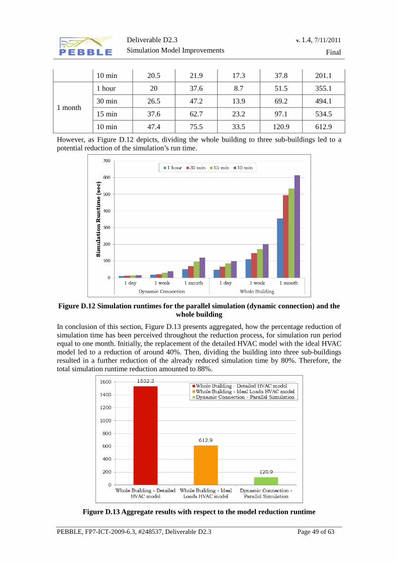
Deliverable D2.3 Simulation Model Improvements
v. 1.4, 7/11/2011
Final
PEBBLE, FP7-ICT-2009-6.3, #248537, Deliverable D2.3 Page 49 of 63
10 min 20.5 21.9 17.3 37.8 201.1
1 month
1 hour 20 37.6 8.7 51.5 355.1
30 min 26.5 47.2 13.9 69.2 494.1
15 min 37.6 62.7 23.2 97.1 534.5
10 min 47.4 75.5 33.5 120.9 612.9
However, as Figure D.12 depicts, dividing the whole building to three sub-buildings led to a potential reduction of the simulation’s run time.
Figure D.12 Simulation runtimes for the parallel simulation (dynamic connection) and the
whole building
In conclusion of this section, Figure D.13 presents aggregated, how the percentage reduction of simulation time has been perceived throughout the reduction process, for simulation run period equal to one month. Initially, the replacement of the detailed HVAC model with the ideal HVAC model led to a reduction of around 40%. Then, dividing the building into three sub-buildings resulted in a further reduction of the already reduced simulation time by 80%. Therefore, the total simulation runtime reduction amounted to 88%.
Figure D.13 Aggregate results with respect to the model reduction runtime
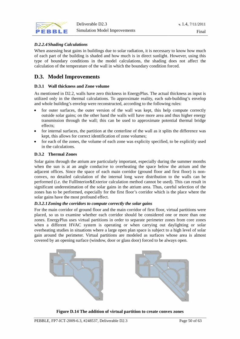
Deliverable D2.3 Simulation Model Improvements
v. 1.4, 7/11/2011
Final
PEBBLE, FP7-ICT-2009-6.3, #248537, Deliverable D2.3 Page 50 of 63
D.2.2.4 Shading Calculations When assessing heat gains in buildings due to solar radiation, it is necessary to know how much of each part of the building is shaded and how much is in direct sunlight. However, using this type of boundary conditions in the model calculations, the shading does not affect the calculation of the temperature of the wall in which the boundary condition forced.
D.3. Model Improvements D.3.1 Wall thickness and Zone volume As mentioned in D2.2, walls have zero thickness in EnergyPlus. The actual thickness as input is utilized only in the thermal calculations. To approximate reality, each sub-building’s envelop and whole building’s envelop were reconstructed, according to the following rules: • for outer surfaces, the outer version of the wall was kept, this help compute correctly
outside solar gains; on the other hand the walls will have more area and thus higher energy transmission through the wall; this can be used to approximate potential thermal bridge effects;
• for internal surfaces, the partition at the centerline of the wall as it splits the difference was kept, this allows for correct identification of zone volumes;
• for each of the zones, the volume of each zone was explicity specified, to be explicitly used in the calculations.
D.3.2 Thermal Zones Solar gains through the atrium are particularly important, especially during the summer months when the sun is at an angle conducive to overheating the space below the atrium and the adjacent offices. Since the space of each main corridor (ground floor and first floor) is non-convex, no detailed calculation of the internal long wave distribution to the walls can be performed (i.e. the FullInterior&Exterior calculation method cannot be used). This can result in significant underestimation of the solar gains in the atrium area. Thus, careful selection of the zones has to be performed, especially for the first floor’s corridor which is the place where the solar gains have the most profound effect. D.3.2.1 Zoning the corridors to compute correctly the solar gains For the main corridor of ground floor and the main corridor of first floor, virtual partitions were placed, so us to examine whether each corridor should be considered one or more than one zones. EnergyPlus uses virtual partitions in order to separate perimeter zones from core zones when a different HVAC system is operating or when carrying out daylighting or solar overheating studies in situations where a large open plan space is subject to a high level of solar gain around the perimeter. Virtual partitions are modeled as surfaces whose area is almost covered by an opening surface (window, door or glass door) forced to be always open.
Figure D.14 The addition of virtual partition to create convex zones
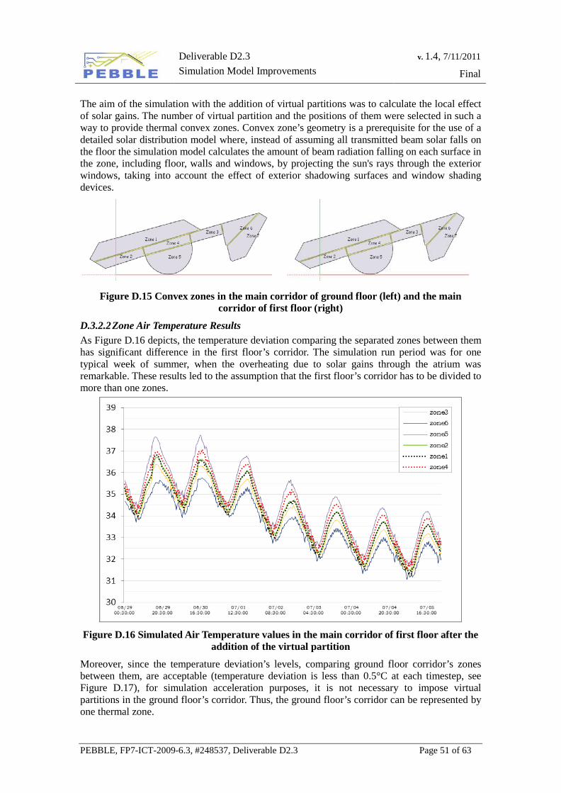
Deliverable D2.3 Simulation Model Improvements
v. 1.4, 7/11/2011
Final
PEBBLE, FP7-ICT-2009-6.3, #248537, Deliverable D2.3 Page 51 of 63
The aim of the simulation with the addition of virtual partitions was to calculate the local effect of solar gains. The number of virtual partition and the positions of them were selected in such a way to provide thermal convex zones. Convex zone’s geometry is a prerequisite for the use of a detailed solar distribution model where, instead of assuming all transmitted beam solar falls on the floor the simulation model calculates the amount of beam radiation falling on each surface in the zone, including floor, walls and windows, by projecting the sun's rays through the exterior windows, taking into account the effect of exterior shadowing surfaces and window shading devices.
Figure D.15 Convex zones in the main corridor of ground floor (left) and the main corridor of first floor (right)
D.3.2.2 Zone Air Temperature Results As Figure D.16 depicts, the temperature deviation comparing the separated zones between them has significant difference in the first floor’s corridor. The simulation run period was for one typical week of summer, when the overheating due to solar gains through the atrium was remarkable. These results led to the assumption that the first floor’s corridor has to be divided to more than one zones.
Figure D.16 Simulated Air Temperature values in the main corridor of first floor after the
addition of the virtual partition
Moreover, since the temperature deviation’s levels, comparing ground floor corridor’s zones between them, are acceptable (temperature deviation is less than 0.5°C at each timestep, see Figure D.17), for simulation acceleration purposes, it is not necessary to impose virtual partitions in the ground floor’s corridor. Thus, the ground floor’s corridor can be represented by one thermal zone.
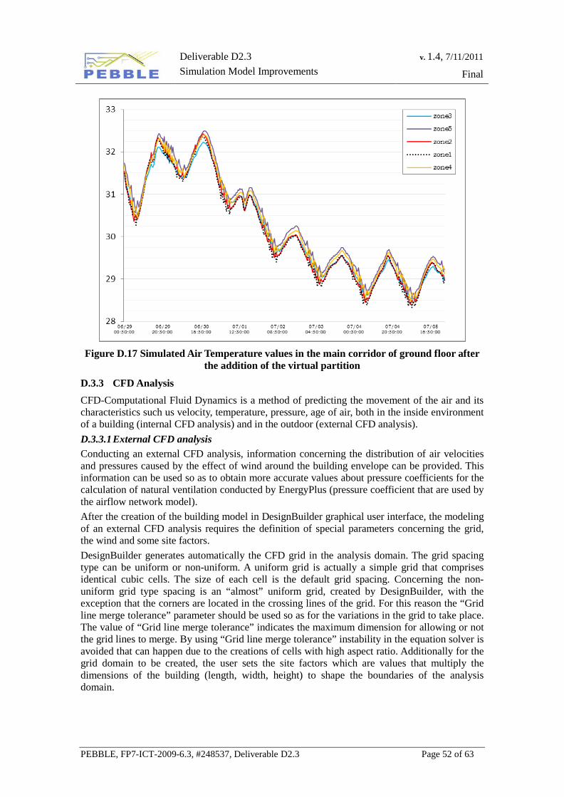
Deliverable D2.3 Simulation Model Improvements
v. 1.4, 7/11/2011
Final
PEBBLE, FP7-ICT-2009-6.3, #248537, Deliverable D2.3 Page 52 of 63
Figure D.17 Simulated Air Temperature values in the main corridor of ground floor after
the addition of the virtual partition
D.3.3 CFD Analysis CFD-Computational Fluid Dynamics is a method of predicting the movement of the air and its characteristics such us velocity, temperature, pressure, age of air, both in the inside environment of a building (internal CFD analysis) and in the outdoor (external CFD analysis). D.3.3.1 External CFD analysis Conducting an external CFD analysis, information concerning the distribution of air velocities and pressures caused by the effect of wind around the building envelope can be provided. This information can be used so as to obtain more accurate values about pressure coefficients for the calculation of natural ventilation conducted by EnergyPlus (pressure coefficient that are used by the airflow network model). After the creation of the building model in DesignBuilder graphical user interface, the modeling of an external CFD analysis requires the definition of special parameters concerning the grid, the wind and some site factors. DesignBuilder generates automatically the CFD grid in the analysis domain. The grid spacing type can be uniform or non-uniform. A uniform grid is actually a simple grid that comprises identical cubic cells. The size of each cell is the default grid spacing. Concerning the non-uniform grid type spacing is an “almost” uniform grid, created by DesignBuilder, with the exception that the corners are located in the crossing lines of the grid. For this reason the “Grid line merge tolerance” parameter should be used so as for the variations in the grid to take place. The value of “Grid line merge tolerance” indicates the maximum dimension for allowing or not the grid lines to merge. By using “Grid line merge tolerance” instability in the equation solver is avoided that can happen due to the creations of cells with high aspect ratio. Additionally for the grid domain to be created, the user sets the site factors which are values that multiply the dimensions of the building (length, width, height) to shape the boundaries of the analysis domain.

Deliverable D2.3 Simulation Model Improvements
v. 1.4, 7/11/2011
Final
PEBBLE, FP7-ICT-2009-6.3, #248537, Deliverable D2.3 Page 53 of 63
Figure D.18 Example of uniform and non-uniform grid spacing type
By default DesignBuilder creates a Cartesian grid which is non-uniform. The lines are parallel with the major axis but because it is a non-uniform grid it can be edited changing the space between the lines. Setting up the external analysis a non-uniform grid was selected with a default grid spacing of 0.5m and a grid line merge tolerance value of 0.1m. The wind velocity was set to 15m/s with 90° direction and suburban exposure. After 4000 iterations the solution is not converged but the residuals for almost all the dependent variables except mass reach 10-4 which is considered to produce quite accurate results.
Figure D.19 Residuals and Cell Monitor
From Figure D.20 until Figure D.24 the distribution of air around the building structures is depicted. The velocity falls into smaller values as the air is moving towards the building. This phenomenon is depicted in blue color for a velocity of 0m/s. The velocity values rise as the distance from the building becomes bigger with the maximum velocity to reach the value of 16.3m/s. Observing Figure D.24 one can easily notice that neighbor buildings act as obstacles in the wind movement.
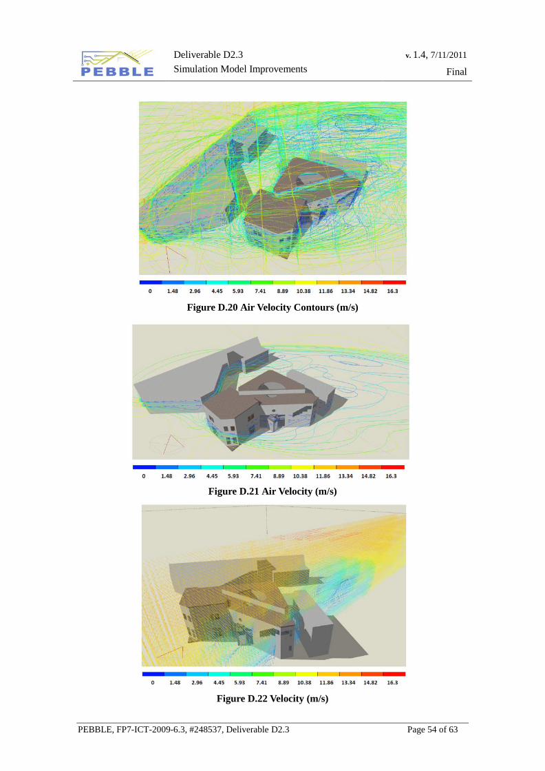
Deliverable D2.3 Simulation Model Improvements
v. 1.4, 7/11/2011
Final
PEBBLE, FP7-ICT-2009-6.3, #248537, Deliverable D2.3 Page 54 of 63
Figure D.20 Air Velocity Contours (m/s)
Figure D.21 Air Velocity (m/s)
Figure D.22 Velocity (m/s)
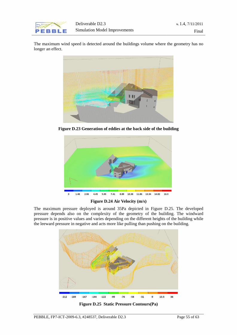
Deliverable D2.3 Simulation Model Improvements
v. 1.4, 7/11/2011
Final
PEBBLE, FP7-ICT-2009-6.3, #248537, Deliverable D2.3 Page 55 of 63
The maximum wind speed is detected around the buildings volume where the geometry has no longer an effect.
Figure D.23 Generation of eddies at the back side of the building
Figure D.24 Air Velocity (m/s)
The maximum pressure deployed is around 35Pa depicted in Figure D.25. The developed pressure depends also on the complexity of the geometry of the building. The windward pressure is in positive values and varies depending on the different heights of the building while the leeward pressure in negative and acts more like pulling than pushing on the building.
Figure D.25 Static Pressure Contours(Pa)
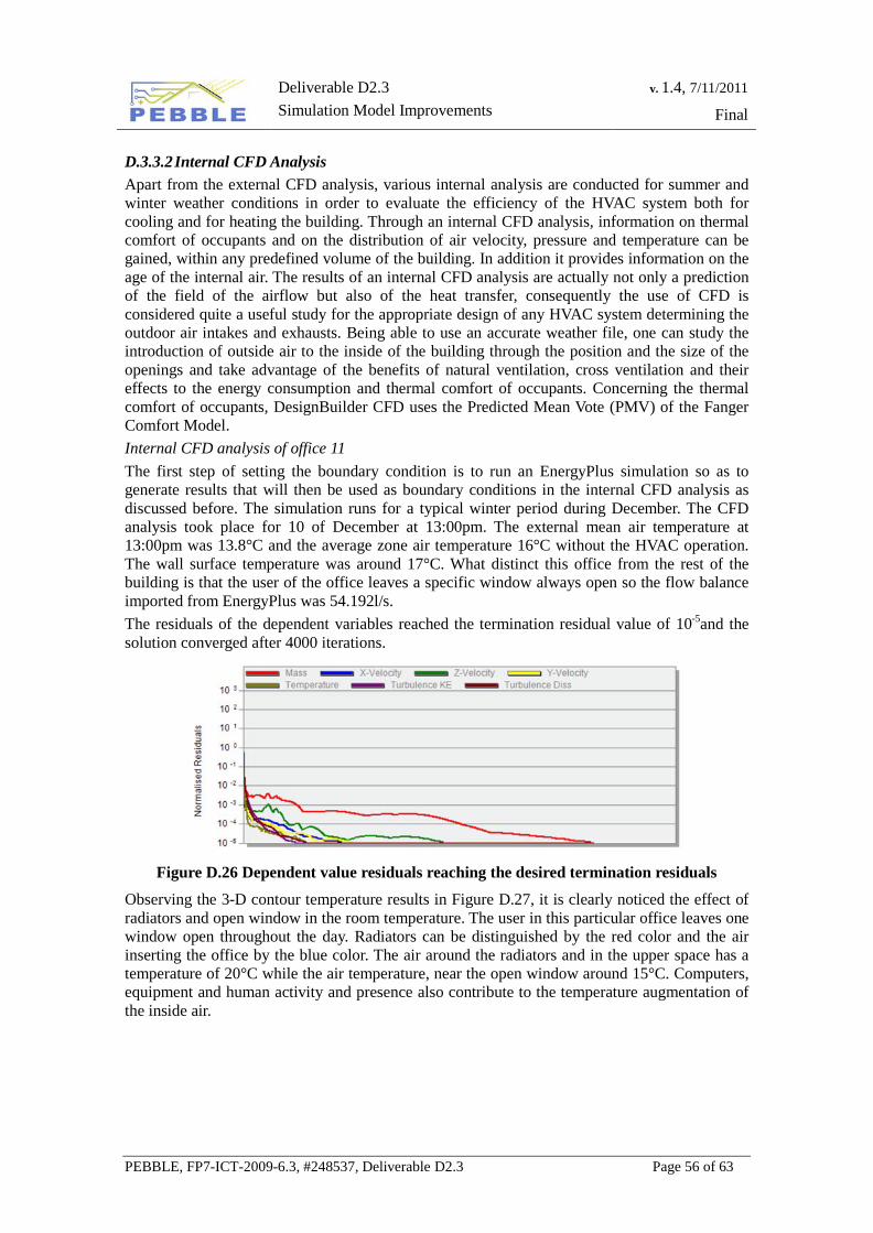
Deliverable D2.3 Simulation Model Improvements
v. 1.4, 7/11/2011
Final
PEBBLE, FP7-ICT-2009-6.3, #248537, Deliverable D2.3 Page 56 of 63
D.3.3.2 Internal CFD Analysis Apart from the external CFD analysis, various internal analysis are conducted for summer and winter weather conditions in order to evaluate the efficiency of the HVAC system both for cooling and for heating the building. Through an internal CFD analysis, information on thermal comfort of occupants and on the distribution of air velocity, pressure and temperature can be gained, within any predefined volume of the building. In addition it provides information on the age of the internal air. The results of an internal CFD analysis are actually not only a prediction of the field of the airflow but also of the heat transfer, consequently the use of CFD is considered quite a useful study for the appropriate design of any HVAC system determining the outdoor air intakes and exhausts. Being able to use an accurate weather file, one can study the introduction of outside air to the inside of the building through the position and the size of the openings and take advantage of the benefits of natural ventilation, cross ventilation and their effects to the energy consumption and thermal comfort of occupants. Concerning the thermal comfort of occupants, DesignBuilder CFD uses the Predicted Mean Vote (PMV) of the Fanger Comfort Model. Internal CFD analysis of office 11 The first step of setting the boundary condition is to run an EnergyPlus simulation so as to generate results that will then be used as boundary conditions in the internal CFD analysis as discussed before. The simulation runs for a typical winter period during December. The CFD analysis took place for 10 of December at 13:00pm. The external mean air temperature at 13:00pm was 13.8°C and the average zone air temperature 16°C without the HVAC operation. The wall surface temperature was around 17°C. What distinct this office from the rest of the building is that the user of the office leaves a specific window always open so the flow balance imported from EnergyPlus was 54.192l/s. The residuals of the dependent variables reached the termination residual value of 10-5and the solution converged after 4000 iterations.
Figure D.26 Dependent value residuals reaching the desired termination residuals
Observing the 3-D contour temperature results in Figure D.27, it is clearly noticed the effect of radiators and open window in the room temperature. The user in this particular office leaves one window open throughout the day. Radiators can be distinguished by the red color and the air inserting the office by the blue color. The air around the radiators and in the upper space has a temperature of 20°C while the air temperature, near the open window around 15°C. Computers, equipment and human activity and presence also contribute to the temperature augmentation of the inside air.
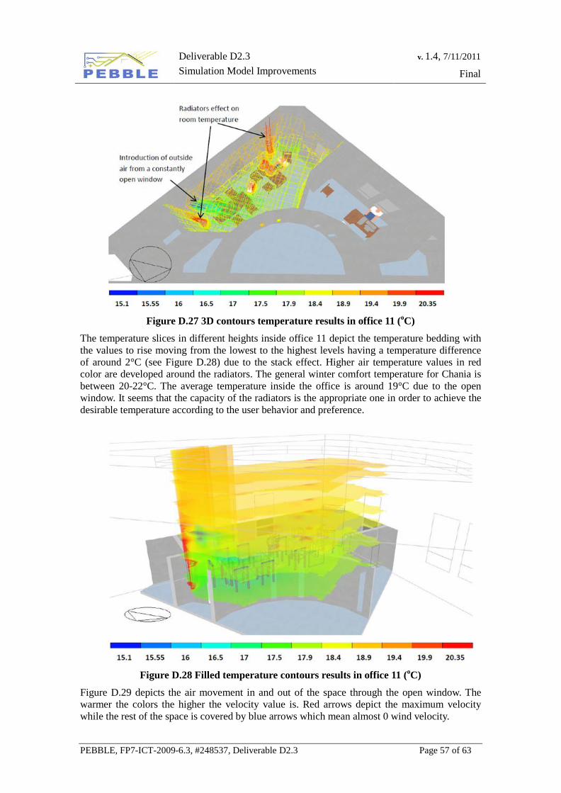
Deliverable D2.3 Simulation Model Improvements
v. 1.4, 7/11/2011
Final
PEBBLE, FP7-ICT-2009-6.3, #248537, Deliverable D2.3 Page 57 of 63
Figure D.27 3D contours temperature results in office 11 (oC)
The temperature slices in different heights inside office 11 depict the temperature bedding with the values to rise moving from the lowest to the highest levels having a temperature difference of around 2°C (see Figure D.28) due to the stack effect. Higher air temperature values in red color are developed around the radiators. The general winter comfort temperature for Chania is between 20-22°C. The average temperature inside the office is around 19°C due to the open window. It seems that the capacity of the radiators is the appropriate one in order to achieve the desirable temperature according to the user behavior and preference.
Figure D.28 Filled temperature contours results in office 11 (oC)
Figure D.29 depicts the air movement in and out of the space through the open window. The warmer the colors the higher the velocity value is. Red arrows depict the maximum velocity while the rest of the space is covered by blue arrows which mean almost 0 wind velocity.
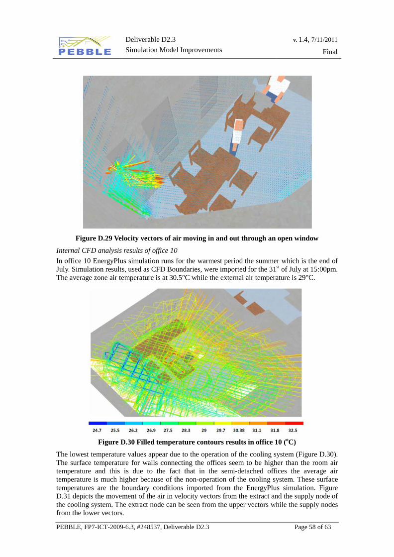
Deliverable D2.3 Simulation Model Improvements
v. 1.4, 7/11/2011
Final
PEBBLE, FP7-ICT-2009-6.3, #248537, Deliverable D2.3 Page 58 of 63
Figure D.29 Velocity vectors of air moving in and out through an open window
Internal CFD analysis results of office 10 In office 10 EnergyPlus simulation runs for the warmest period the summer which is the end of July. Simulation results, used as CFD Boundaries, were imported for the 31st of July at 15:00pm. The average zone air temperature is at 30.5°C while the external air temperature is 29°C.
Figure D.30 Filled temperature contours results in office 10 (oC)
The lowest temperature values appear due to the operation of the cooling system (Figure D.30). The surface temperature for walls connecting the offices seem to be higher than the room air temperature and this is due to the fact that in the semi-detached offices the average air temperature is much higher because of the non-operation of the cooling system. These surface temperatures are the boundary conditions imported from the EnergyPlus simulation. Figure D.31 depicts the movement of the air in velocity vectors from the extract and the supply node of the cooling system. The extract node can be seen from the upper vectors while the supply nodes from the lower vectors.
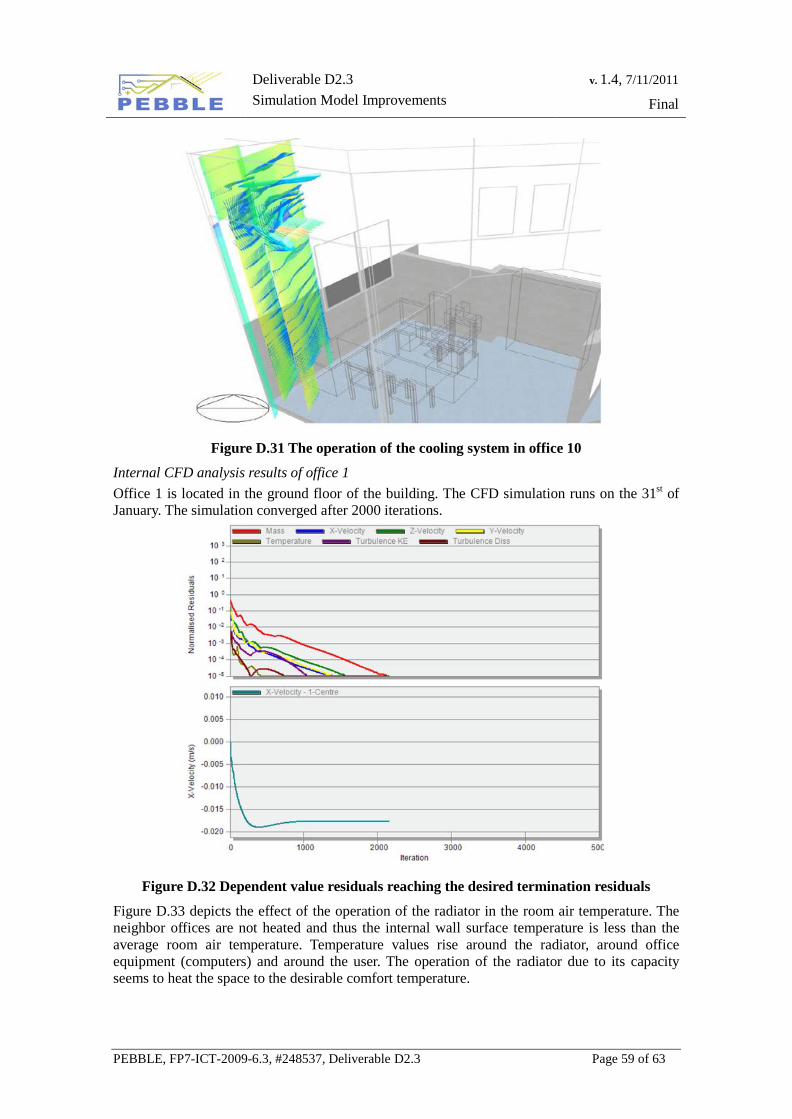
Deliverable D2.3 Simulation Model Improvements
v. 1.4, 7/11/2011
Final
PEBBLE, FP7-ICT-2009-6.3, #248537, Deliverable D2.3 Page 59 of 63
Figure D.31 The operation of the cooling system in office 10
Internal CFD analysis results of office 1 Office 1 is located in the ground floor of the building. The CFD simulation runs on the 31st of January. The simulation converged after 2000 iterations.
Figure D.32 Dependent value residuals reaching the desired termination residuals
Figure D.33 depicts the effect of the operation of the radiator in the room air temperature. The neighbor offices are not heated and thus the internal wall surface temperature is less than the average room air temperature. Temperature values rise around the radiator, around office equipment (computers) and around the user. The operation of the radiator due to its capacity seems to heat the space to the desirable comfort temperature.
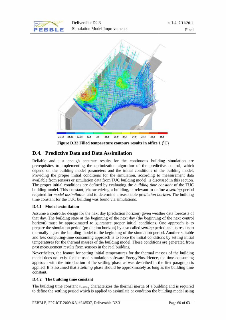
Deliverable D2.3 Simulation Model Improvements
v. 1.4, 7/11/2011
Final
PEBBLE, FP7-ICT-2009-6.3, #248537, Deliverable D2.3 Page 60 of 63
Figure D.33 Filled temperature contours results in office 1 (oC)
D.4. Predictive Data and Data Assimilation Reliable and just enough accurate results for the continuous building simulation are prerequisites to implementing the optimization algorithm of the predictive control, which depend on the building model parameters and the initial conditions of the building model. Providing the proper initial conditions for the simulation, according to measurement data available from sensors or simulation data from TUC building model, is discussed in this section. The proper initial conditions are defined by evaluating the building time constant of the TUC building model. This constant, characterizing a building, is relevant to define a settling period required for model assimilation and to determine a reasonable prediction horizon. The building time constant for the TUC building was found via simulations.
D.4.1 Model assimilation Assume a controller design for the next day (prediction horizon) given weather data forecasts of that day. The building state at the beginning of the next day (the beginning of the next control horizon) must be approximated to guarantee proper initial conditions. One approach is to prepare the simulation period (prediction horizon) by a so called settling period and its results to thermally adjust the building model to the beginning of the simulation period. Another suitable and less computing-time consuming approach is to force the initial conditions by setting initial temperatures for the thermal masses of the building model. These conditions are generated from past measurement results from sensors in the real building. Nevertheless, the feature for setting initial temperatures for the thermal masses of the building model does not exist for the used simulation software EnergyPlus. Hence, the time consuming approach with the introduction of the settling phase as was described in the first paragraph is applied. It is assumed that a settling phase should be approximately as long as the building time constant.
D.4.2 The building time constant The building time constant τbuilding characterizes the thermal inertia of a building and is required to define the settling period which is applied to assimilate or condition the building model using
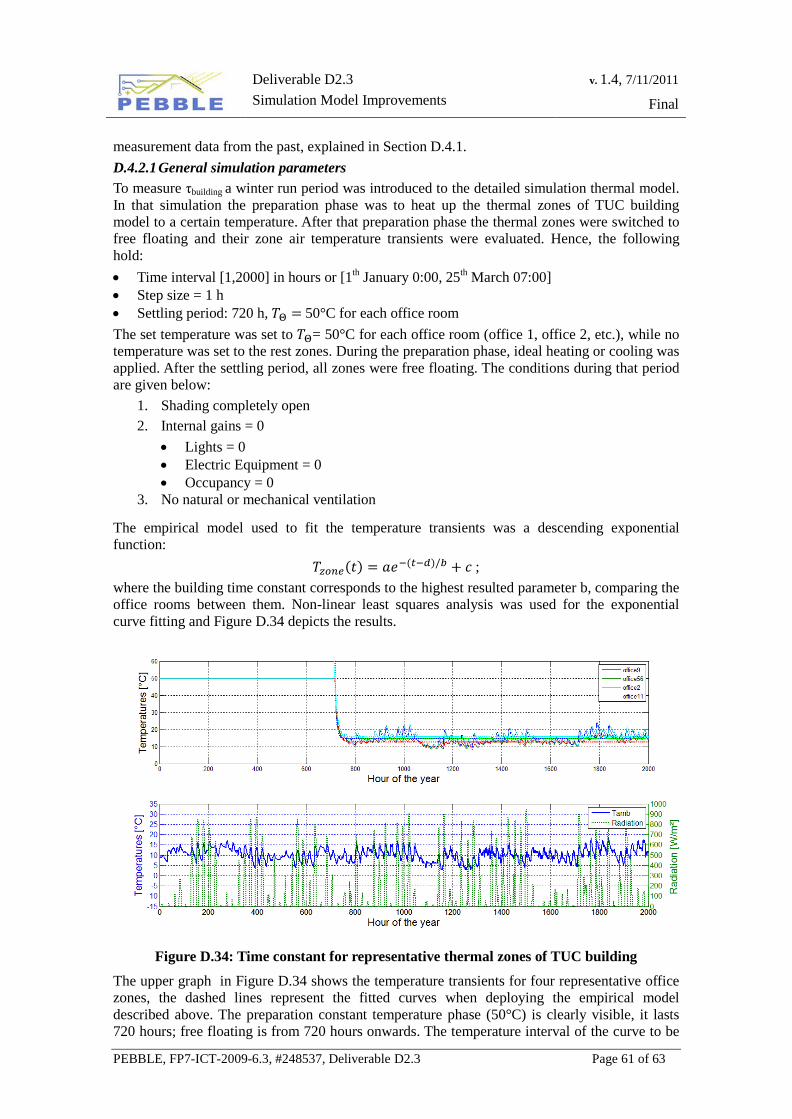
Deliverable D2.3 Simulation Model Improvements
v. 1.4, 7/11/2011
Final
PEBBLE, FP7-ICT-2009-6.3, #248537, Deliverable D2.3 Page 61 of 63
measurement data from the past, explained in Section D.4.1. D.4.2.1 General simulation parameters To measure τbuilding a winter run period was introduced to the detailed simulation thermal model. In that simulation the preparation phase was to heat up the thermal zones of TUC building model to a certain temperature. After that preparation phase the thermal zones were switched to free floating and their zone air temperature transients were evaluated. Hence, the following hold: • Time interval [1,2000] in hours or [1th January 0:00, 25th March 07:00] • Step size = 1 h • Settling period: 720 h, 𝑇Θ = 50°C for each office room The set temperature was set to 𝑇Θ= 50°C for each office room (office 1, office 2, etc.), while no temperature was set to the rest zones. During the preparation phase, ideal heating or cooling was applied. After the settling period, all zones were free floating. The conditions during that period are given below:
1. Shading completely open 2. Internal gains = 0
• Lights = 0 • Electric Equipment = 0 • Occupancy = 0
3. No natural or mechanical ventilation
The empirical model used to fit the temperature transients was a descending exponential function:
𝑇𝑧𝑜𝑛𝑒(𝑡) = 𝑎𝑒−(𝑡−𝑑)/𝑏 + 𝑐 ; where the building time constant corresponds to the highest resulted parameter b, comparing the office rooms between them. Non-linear least squares analysis was used for the exponential curve fitting and Figure D.34 depicts the results.
Figure D.34: Time constant for representative thermal zones of TUC building
The upper graph in Figure D.34 shows the temperature transients for four representative office zones, the dashed lines represent the fitted curves when deploying the empirical model described above. The preparation constant temperature phase (50°C) is clearly visible, it lasts 720 hours; free floating is from 720 hours onwards. The temperature interval of the curve to be
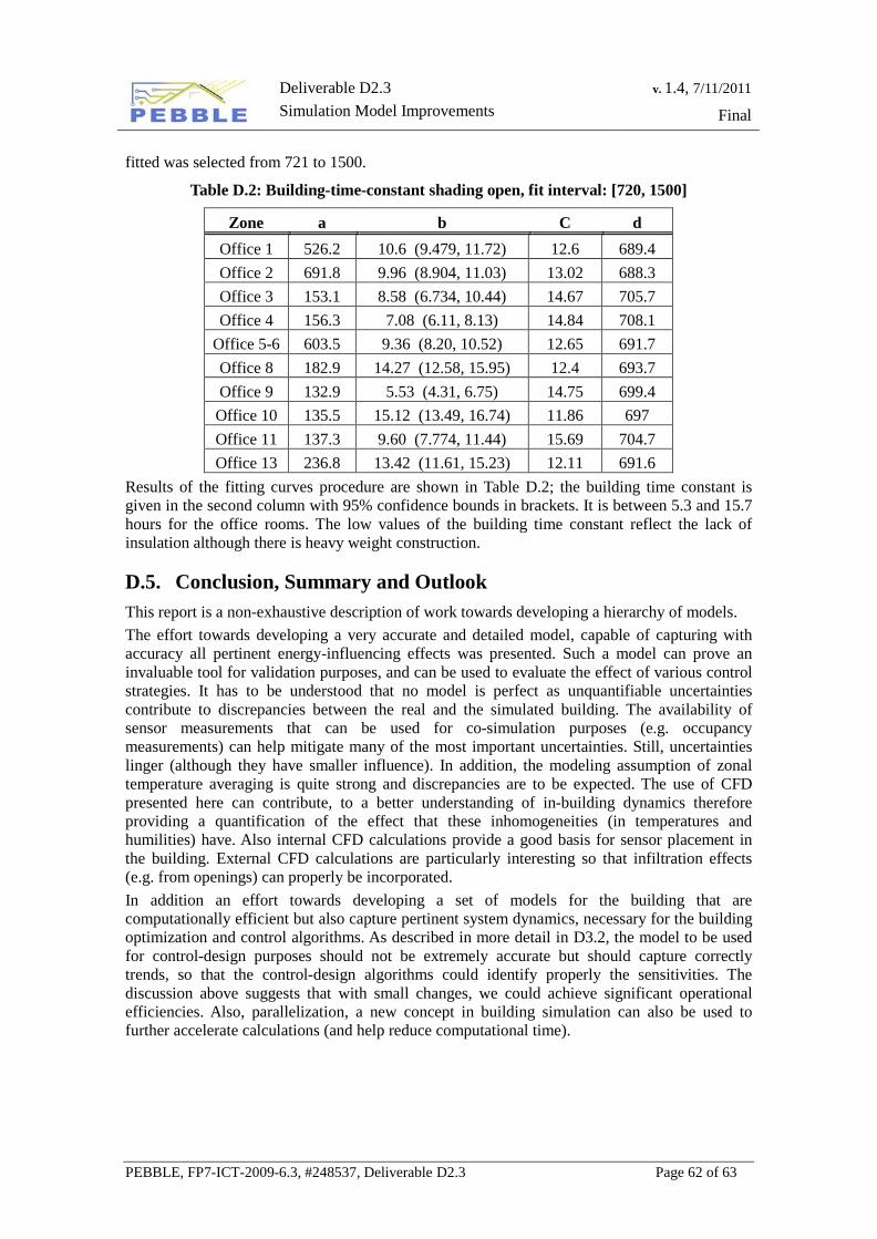
Deliverable D2.3 Simulation Model Improvements
v. 1.4, 7/11/2011
Final
PEBBLE, FP7-ICT-2009-6.3, #248537, Deliverable D2.3 Page 62 of 63
fitted was selected from 721 to 1500.
Table D.2: Building-time-constant shading open, fit interval: [720, 1500]
Zone a b C d Office 1 526.2 10.6 (9.479, 11.72) 12.6 689.4 Office 2 691.8 9.96 (8.904, 11.03) 13.02 688.3 Office 3 153.1 8.58 (6.734, 10.44) 14.67 705.7 Office 4 156.3 7.08 (6.11, 8.13) 14.84 708.1
Office 5-6 603.5 9.36 (8.20, 10.52) 12.65 691.7 Office 8 182.9 14.27 (12.58, 15.95) 12.4 693.7 Office 9 132.9 5.53 (4.31, 6.75) 14.75 699.4 Office 10 135.5 15.12 (13.49, 16.74) 11.86 697 Office 11 137.3 9.60 (7.774, 11.44) 15.69 704.7 Office 13 236.8 13.42 (11.61, 15.23) 12.11 691.6
Results of the fitting curves procedure are shown in Table D.2; the building time constant is given in the second column with 95% confidence bounds in brackets. It is between 5.3 and 15.7 hours for the office rooms. The low values of the building time constant reflect the lack of insulation although there is heavy weight construction.
D.5. Conclusion, Summary and Outlook This report is a non-exhaustive description of work towards developing a hierarchy of models. The effort towards developing a very accurate and detailed model, capable of capturing with accuracy all pertinent energy-influencing effects was presented. Such a model can prove an invaluable tool for validation purposes, and can be used to evaluate the effect of various control strategies. It has to be understood that no model is perfect as unquantifiable uncertainties contribute to discrepancies between the real and the simulated building. The availability of sensor measurements that can be used for co-simulation purposes (e.g. occupancy measurements) can help mitigate many of the most important uncertainties. Still, uncertainties linger (although they have smaller influence). In addition, the modeling assumption of zonal temperature averaging is quite strong and discrepancies are to be expected. The use of CFD presented here can contribute, to a better understanding of in-building dynamics therefore providing a quantification of the effect that these inhomogeneities (in temperatures and humilities) have. Also internal CFD calculations provide a good basis for sensor placement in the building. External CFD calculations are particularly interesting so that infiltration effects (e.g. from openings) can properly be incorporated. In addition an effort towards developing a set of models for the building that are computationally efficient but also capture pertinent system dynamics, necessary for the building optimization and control algorithms. As described in more detail in D3.2, the model to be used for control-design purposes should not be extremely accurate but should capture correctly trends, so that the control-design algorithms could identify properly the sensitivities. The discussion above suggests that with small changes, we could achieve significant operational efficiencies. Also, parallelization, a new concept in building simulation can also be used to further accelerate calculations (and help reduce computational time).
Deliverable D2.3 Simulation Model Improvements
v. 1.4, 7/11/2011
Final
PEBBLE, FP7-ICT-2009-6.3, #248537, Deliverable D2.3 Page 63 of 63
References [1] DIN EN 13779, Ventilation for non-residential buildings – Performance requirements for
ventilation and room-conditioning systems, Beuth Verlag, 2007. [2] Angela Dröscher, Martin Pichler, Hermann Schranzhofer, Ana Constantin, N. Exizidou,
G. Giannakis, and D. Rovas. D2.2 Validation Results of the Models (Draft Version). Technical report, 2011.
[3] Frauke Oldewurtel, Dimitrios Gyalistras, Markus Gwerder, Colin N. Jones, Alessandra Parisio, Vanessa Stauch, Beat Lehmann, and Manfred Morari. Increasing energy efficiency in building climate control using weather forecasts and model predictive control. 2010.
[4] G. Kontes, G. Giannakis, E. Kosmatopoulos, and D.V. Rovas. PEBBLE Deliverable 3.2. Technical report, Technical University of Crete, 2011.
[5] DIN 18599, Energy efficiency of buildings – Calculation of the net, final and primary energy demand for heating, cooling, ventilation, domestic hot water and lighting, part 1, Beuth Verlag, 2007
[6] VDI 2078, Cooling Load Calculation of Air-conditioned Rooms (VDI Cooling Load Regulations), Beuth Verlag, 1996
[7] MATLAB, Version 2010b, MathWorks, 2010 [8] BCVTB, Building Controls Virtual Test Bed, Lawrence-Berkley National Laboratory. [9] G. Kontes, G. Giannakis, E. Kosmatopoulos and D.V. Rovas. PEBBLE Deliverable 3.3.
Technical report, Technical University of Crete, 2011.