pedestrian safety analysis through effective exposure
TRANSCRIPT

University of Central Florida University of Central Florida
STARS STARS
Electronic Theses and Dissertations, 2004-2019
2017
Pedestrian Safety Analysis through Effective Exposure Measures Pedestrian Safety Analysis through Effective Exposure Measures
and Examination of Injury Severity and Examination of Injury Severity
Md Imran Shah University of Central Florida
Part of the Civil Engineering Commons
Find similar works at: https://stars.library.ucf.edu/etd
University of Central Florida Libraries http://library.ucf.edu
This Masters Thesis (Open Access) is brought to you for free and open access by STARS. It has been accepted for
inclusion in Electronic Theses and Dissertations, 2004-2019 by an authorized administrator of STARS. For more
information, please contact [email protected].
STARS Citation STARS Citation Shah, Md Imran, "Pedestrian Safety Analysis through Effective Exposure Measures and Examination of Injury Severity" (2017). Electronic Theses and Dissertations, 2004-2019. 5365. https://stars.library.ucf.edu/etd/5365

PEDESTRIAN SAFETY ANALYSIS THROUGH EFFECTIVE EXPOSURE
MEASURES AND EXAMINATION OF INJURY SEVERITY
by
MD IMRAN SHAH
B.S. Bangladesh University of Engineering & Technology, 2014
A thesis submitted in partial fulfillment of the requirements
for the degree of Master of Science
in the Department of Civil, Environmental and Construction Engineering
in the College of Engineering and Computer Science
at the University of Central Florida
Orlando, Florida
Spring Term
2017
Major Professor: Mohamed A. Abdel-Aty

ii
© 2017 Md Imran Shah

iii
ABSTRACT
Pedestrians are considered the most vulnerable road users who are directly exposed to
traffic crashes. In 2014, there were 4,884 pedestrians killed and 65,000 injured in the United
States. Pedestrian safety is a growing concern in the development of sustainable transportation
system. But often it is found that safety analysis suffers from lack of accurate pedestrian trip
information. In such cases, determining effective exposure measures is the most appropriate
safety analysis approach. Also it is very important to clearly understand the relationship between
pedestrian injury severity and the factors contributing to higher injury severity. Accurate safety
analysis can play a vital role in the development of appropriate safety countermeasures and
policies for pedestrians.
Since pedestrian volume data is the most important information in safety analysis but
rarely available, the first part of the study aims at identifying surrogate measures for pedestrian
exposure at intersections. A two-step process is implemented: the first step is the development of
Tobit and Generalized Linear Models for predicting pedestrian trips (i.e., exposure models). In
the second step, Negative Binomial and Zero Inflated Negative Binomial crash models were
developed using the predicted pedestrian trips. The results indicate that among various exposure
models the Tobit model performs the best in describing pedestrian exposure. The identified
exposure relevant factors are the presence of schools, car-ownership, pavement condition,
sidewalk width, bus ridership, intersection control type and presence of sidewalk barrier. The t-
test and Wilcoxon signed-rank test results show that there is no significant difference between
the observed and the predicted pedestrian trips. The process implemented can help in estimating
reliable safety performance functions even when pedestrian trip data is unavailable.

iv
The second part of the study focuses on analyzing pedestrian injury severity for the nine
counties in Central Florida. The study region covers the Orlando area which has the second-
worst pedestrian death rate in the country. Since the dependent variable ‘Injury’ is ordinal, an
‘Ordered Logit’ model was developed to identify the factors of pedestrian injury severity. The
explanatory variables can be classified as pedestrian/driver characteristics (e.g., age, gender,
etc.), roadway traffic and geometric conditions (e.g.: shoulder presence, roadway speed etc.) and
crash environment (e.g., light, road surface, work zone, etc.) characteristics. The results show
that drug/alcohol involvement, pedestrians in a hurry, roadway speed limit 40 mph or more, dark
condition (lighted and unlighted) and presence of elder pedestrians are the primary contributing
factors of severe pedestrian crashes in Central Florida. Crashes within the presence of
intersections and local roads result in lower injury severity. The area under the ROC (Receiver
Operating Characteristic) curve has a value of 0.75 that indicates the model performs reasonably
well. Finally the study validated the model using k-fold cross validation method. The results
could be useful for transportation officials for further pedestrian safety analysis and taking the
appropriate safety interventions.
Walking is cost-effective, environmentally friendly and possesses significant health
benefits. In order to get these benefits from walking, the most important task is to ensure safer
roads for pedestrians.

v
ACKNOWLEDGMENTS
I would first like to express my gratitude to my thesis advisor and the committee chair
Professor Dr. Mohamed Abdel-Aty; Chair, Department of Civil, Environmental & Construction
Engineering, Univeristy of Central Florida. He kept the door always open whenever there arose
any difficulty in conducting the study or writing the thesis manual. The continous monitoring of
the work and the valauble inspiration from Professor Abdel-Aty made it possible to complete the
study successfully.
I must acknowledge the relentless support and guidance provided by Dr. Jaeyoung Lee in
conducting the research work. Withuout the literature and technical support provided by Dr. Lee,
it was hardly possible to finish the study. I would like to thank the thesis committee members Dr.
Naveen Eluru and Dr. Jaeyoung Lee for their valuable time and review. Also I would like to
thank all my wonderful colleaugues for their support and inspiration that helped me keeping the
right track. I have learned a lot during my acdemic life at UCF from this tranporation research
group. I’m grateful to the University of Central Florida, College of Graduate Studies for their
financial support and amendments they provided in pursuing the Masters degree.
Finally, I must express my very profound gratitude to my parents, my wife and friends
for providing me with unfailing support and continuous encouragement. Special thanks goes to
my mother who amzingly guided and inspired me throughout my whole life. This
accomplishment would not have been possible without her invaluable efforts.
Thank you
Md Imran Shah

vi
TABLE OF CONTENTS
LIST OF FIGURES ..................................................................................................................... viii
LIST OF TABLES ......................................................................................................................... ix
LIST OF ABBREVIATIONS ......................................................................................................... x
CHAPTER 1. INTRODUCTION ................................................................................................... 1
1.1 Overview ............................................................................................................................... 1
1.2 Pedestrian Exposure Measurement ....................................................................................... 2
1.3 Pedestrian Injury Severity Analysis ...................................................................................... 4
1.4 Research Objectives & Tasks Performed .............................................................................. 5
1.5 Thesis Outline ....................................................................................................................... 7
CHAPTER 2. LITERATURE REVIEW ........................................................................................ 9
2.1 Brief Statistics of Pedestrian Crash Representing the Current Situation .............................. 9
2.2 Importance of Safe Walking ............................................................................................... 13
2.3 Studies Related to Pedestrian Exposure .............................................................................. 14
2.4 Review of Modeling Techniques & Variables for the Exposure Study .............................. 16
2.5 Studies on Pedestrian Injury Severity ................................................................................. 18
2.6 Appropriate Modeling Technique for Injury Severity ........................................................ 19
CHAPTER 3. RESEARCH METHODOLOGIES ....................................................................... 21
3.1 Methods Used for Exposure Models ................................................................................... 21
3.2 Statistical Test to Compare Observed and Predicted Pedestrian Trips ............................... 25
3.3 Methods Used to Develop Crash Models ............................................................................ 26
3.4 Methodologies Used in Injury Severity Analysis ............................................................... 28
3.5 k-fold Cross Validation ....................................................................................................... 30
CHAPTER 4. DATA PREPARATION ........................................................................................ 31
4.1 Data Collection Source for the Exposure Analysis ............................................................. 31
4.2 Data Processing for the Exposure Analysis ........................................................................ 34

vii
4.3 Data Processing for Injury Severity Analysis ..................................................................... 37
CHAPTER 5. DATA ANALYSES AND MODEL RESULTS ................................................... 40
5.1 Exposure Analysis Results .................................................................................................. 40
5.2 Statistical Test Results Comparing Observed & Predicted Pedestrian Trips ...................... 45
5.3 Results of the Crash Models Developed using Predicted Pedestrian Trips ........................ 46
5.4 Injury Severity Analysis Results ......................................................................................... 47
5.5 k fold cross validation result ............................................................................................... 54
CHAPTER 6. CONCLUSIONS AND RECOMMENDATIONS ................................................ 56
REFERENCES .............................................................................................................................. 61

viii
LIST OF FIGURES
Figure 1. Exposed Pedestrian (source: Joe Raedle / Getty Images) ............................................... 2
Figure 2. Pedestrian Crossing Intersection (source: Chris Urso/Tribune) ...................................... 3
Figure 3. Pedestrian Struck by Car (source: KMGH / The Denver Channel) ................................ 4
Figure 4. Thesis Organization Flow Chart ...................................................................................... 8
Figure 5. Pedestrian Death Rate over Last Decade (source: FARS) ............................................ 10
Figure 6. Pedestrian Crash Statistics (source: The Miley Legal Group/NHTSA) ........................ 11
Figure 7. Florida is the most Dangerous State for Pedestrians (source: FARS/obrella.com) ....... 12
Figure 8. Safe Walking Tips (source: St. Paul Public Schools Transportation Department) ....... 13
Figure 9. Histogram of Pedestrian Trips Distribution .................................................................. 34
Figure 10. Histogram of Pedestrian Trips Distribution ................................................................ 35
Figure 11. Crash mapping using GIS ............................................................................................ 36
Figure 12. Intersection near School with Crossing Guard (source: Dreams-time) ....................... 42
Figure 13. Public Transit in Central Florida (source: LYNX) ...................................................... 43
Figure 14. Pedestrian Sidewalk Barrier (source: goldengate.org) ................................................ 44
Figure 15. Alcohol leads to Fatality (source: Mother Jones / NHTSA) ....................................... 50
Figure 16. Pedestrian under Dark Condition (Source: Getty Images) .......................................... 51
Figure 17. Pedestrians walking in a Hurry (source: Inhabitat) ..................................................... 52
Figure 18. Impact of vehicle Speed on Pedestrian Fatality (Source: saferspeedarea.org.nz) ....... 53
Figure 19. Elder Pedestrian Requires Special Assistant (source: Chip Latherland/NY Times) ... 54

ix
LIST OF TABLES
Table 1. List of Variables and Data Sources................................................................................. 32
Table 2. Pearson correlations coefficient of some selected explanatory variables ....................... 36
Table 3. Variables Available for Injury Severity Analysis ........................................................... 38
Table 4. Comparison of the exposure models developed ............................................................. 41
Table 5. Tobit model result (Best exposure model obtained) ....................................................... 41
Table 6. Statistical test to compare observed and predicted pedestrian trips................................ 45
Table 7. NB crash model using predicted trips from exposure model.......................................... 46
Table 8. NB crash model using original pedestrian trips as exposure .......................................... 46
Table 9. Comparison of developed crash models ......................................................................... 47
Table 10. Model Fit Statistics of ‘Ordered Logit’ Model ............................................................. 48
Table 11. Significant Explanatory Variables of Injury Severity Analysis .................................... 48
Table 12. Association of Predicted Probabilities and Observed Response .................................. 48
Table 13. c Statistics for 10 fold Cross Validation ....................................................................... 55
Table 14. Lift Table Created for Injury Severity Profile .............................................................. 55
Table 15. Engineering/ITS Based Safety Countermeasures (FHWA, 2014)................................ 58

x
LIST OF ABBREVIATIONS
AIC Akaike Information Criterion
AUC Area Under Curve
BIC Bayesian Information Criterion
CARS Crash Analysis Reporting System
DHSMV Department of Highway Safety & Motor Vehicle
FDOT Florida Department of Transportation
FHWA Federal Highway Administration
FT Feet
GLM Generalized Linear Modeling
IIHS Insurance Institute for Highway Safety
ITS Intelligent Transportation System
MAD Mean Absolute Deviation
MLE Maximum Likelihood Estimation
MPH Mile Per Hour
MSE Mean Square Error
NB Negative Binomial

xi
NHTSA National Highway Traffic Safety Administration
NZTA New Zealand Transport Agency
OLS Ordinary Least Squares
PCA Principal Component Analysis
RMSE Root Mean Square Error
ROC Receiver Operating Characteristics
T4A Transportation for America
TRB Transportation Research Board
UCF University of Central Florida
US United States
WHO World Health Organization
ZINB Zero Inflated Negative Binomial

1
CHAPTER 1. INTRODUCTION
1.1 Overview
Being classified as vulnerable road users, pedestrians are recognized as the worst victims
of traffic crashes. In 2014, there were 4,884 pedestrians killed and 65,000 injured on roads that
indicate on average, a pedestrian was killed every 2 hours and injured every 8 minutes (NHTSA,
2014). The proportion of pedestrian fatalities has steadily increased from 11% to 14% over the
past decade. The number describes the importance of addressing the safety of pedestrians and
raising awareness among the people about safe walking. Walking is one of the basic activities in
human daily life that can contribute important health and economic benefits. According to the
New Zealand Transport Agency the total health benefit of walking was estimated to be $2.6 per
each kilometer walked (NZTA, 2010; Rahul and Verma, 2013). Walking is cost-effective and
environmentally friendly that can reduce rates of chronic disease and ameliorate rising health
care costs (Lee and Buchner, 2008). The extensive research in the sustainable transportation
systems improvement increased the significance of pedestrian safety and sustainable pedestrian
facilities. Several studies have shown pedestrian volume to be a significant measure for
pedestrian exposure estimation (Raford and Ragland, 2005; Tobey et al., 1983). But in many
studies pedestrian exposure has been observed as a measurement issue in the development of
pedestrian safety models. So it has been a challenge for the researchers to carry out proper safety
analysis due to the unavailability or inaccurate pedestrian volume data. Again the injury severity
levels of pedestrians are relatively high compared to those in motor vehicle crashes. The reason
behind this is unlike the passengers or drivers in motor vehicle crashes, pedestrians are directly
exposed to the impact of traffic crashes. Therefore, the significance of understanding relationship
between pedestrian injury severity level and the factors must be addressed by the traffic

2
engineers, planners and decision makers in order develop proper safety countermeasures as well
as education and enforcement interventions. Individual region based safety analysis approach
along with statewide policy analysis can help improve the safety of pedestrians.
1.2 Pedestrian Exposure Measurement
It has been a common practice in exposure science and environmental epidemiology to
collect detailed and precise micro-environment data in which an individual stays or moves
(Lassarre et al., 2007). Scientific crash risk analysis incorporates individual’s activity-travel
pattern as an exposure measurement. The underlying theory is that crash data as points-in-
networks along with disaggregate exposure data can identify hazardous crash locations where
road safety improvements can be made.
Figure 1. Exposed Pedestrian (source: Joe Raedle / Getty Images)
The first part of the study aims at identifying the exposure factors to pedestrian crashes at
intersections. Intersections are among the significant pedestrian crash occurring locations. In
2014 there were 923 (18.9%) pedestrian fatalities occurred at or near intersections in the US. It is

3
obvious that the number of people walking on the road (i.e., pedestrian trips) is one of the best
measures of exposure for pedestrians (Davis and Braaksma, 1988; Qin and Ivan, 2001; Lam et
al., 2014). However, it is difficult to continuously measure the pedestrian trips at all locations as
it involves using significant amount of resources. This study aims at addressing the situation
when it is difficult to collect pedestrian trip data. The objective of this study is to analyze
surrogate measures for pedestrian exposure to traffic crashes at intersections including the use of
socio-demographic, land-use and geometric characteristics of the surrounding environment. The
two-step process implemented in the study involves developing the exposure models first and
then the crash models.
Figure 2. Pedestrian Crossing Intersection (source: Chris Urso/Tribune)
The exposure models were developed using Tobit and Generalized Linear Modeling
(GLM) methods that predict the pedestrian trips. After identifying the best exposure model,
Negative Binomial (NB) and Zero Inflated Negative Binomial (ZINB) crash models were
developed using the predicted pedestrian trips as an exposure variable. The method can be
described as an integrated pedestrian safety analysis around intersections (micro-level) with

4
macro-level data from census block groups. The study contributes to the research area of
pedestrian safety through identifying the best exposure for pedestrian crashes at intersections and
developing a process of safety analysis for locations where pedestrian data is not available.
Proper knowledge of exposure factors can help transportation officials to develop safer roads for
pedestrians through implementing the right safety interventions.
1.3 Pedestrian Injury Severity Analysis
The second part of the study focuses on analyzing pedestrian injury severity for the nine
counties in Central Florida. The nine counties are Marion, Sumter, Lake, Seminole, Orange,
Osceola, Polk, Hardee and Highlands. Central Florida has been known as a high risk zone for the
people walking on roads. Every year more than 1100 Central Floridians are struck by cars and at
least 900 suffer what police call ‘incapacitating’ injuries. The number of fatality ranges from 80
to 100 each year (FL-DHSMV, 2011-2015). It must be mentioned that the transportation system
in Central Florida is mostly auto oriented. Public transportation system is also not much popular
in this region. Very few people are seen walking on the road for purely commuting purpose.
Figure 3. Pedestrian Struck by Car (source: KMGH / The Denver Channel)

5
Despite these facts the death rate of pedestrian seems to be rising each year. The study
region covers the Orlando area which has the second worst pedestrian death rate in the country.
In this study an ‘Ordered Logit’ model was developed to identify the pedestrian injury severity
factors since the dependent variable ‘Injury’ is ordinal in nature. The explanatory variables can
be classified as pedestrian/driver characteristics (e.g., age, gender, etc.), roadway traffic and
geometric conditions (e.g.: shoulder presence, roadway speed etc.) and crash environment (e.g.,
light, road surface, work zone, etc.) characteristics. The results show that drug/alcohol
involvement, pedestrians in a hurry, roadway speed limit more than 40 mph, dark condition
(lighted and unlighted) and presence of elder pedestrians are the primary contributing factors of
severe pedestrian crashes in Central Florida. On the other hand crashes occuring within the
presence of intersections and local roads are associated with lower injury severity. The area
under the ROC (Receiver Operating Characteristic) curve has a value of 0.75 that indicates the
model performs reasonably well. Finally the study validated the model using k-fold cross
validation method. The outcome of the validation shows that the validation dataset has a ROC
value of 0.72 (close to original c value) that indicates the model is good enough in describing the
relationship between injury severity and the factors contributing to it. The results could be useful
for transportation officials for further pedestrian safety analysis and taking the appropriate safety
interventions for the pedestrian crashes in Central Florida. The study also recommends some
safety countermeasures that can be adopted to make the traffic system in Central Florida more
pedestrian friendly.
1.4 Research Objectives & Tasks Performed
Based on the understanding of the pedestrian safety problem the main objectives of the study
can be listed as follows:

6
Identification of pedestrian exposure factors at intersection using surrogate safety
analysis.
Developing pedestrian safety analysis process where pedestrian volume data is not
available.
Modeling pedestrian crash risk at intersection including socio-demographic, land use
pattern and geometric characteristics of the surrounding environment.
Application of Zero Inflated Negative Binomial model in census block group level
(MICROSCOPIC) pedestrian safety analysis.
Identification of significant factors contributing to severe pedestrian injuries in the
Central Florida region.
Application of ‘Ordered Logit’ model in injury severity analysis in the Central Florida
using the FDOT crash database.
Identification of appropriate pedestrian safety improvement countermeasures based on
the analysis results.
In order to achieve these objectives the following tasks were performed:
Collection of socio-demographic, geometric and land use data of the area under analysis.
The crash data were obtained from FDOT crash database.
Development of statistical models such as Tobit or Generalized Linear model for
exposure, Negative Binomial or Zero Inflated Negative Binomial for crash models,
Ordered Logit for injury severity.
Application of statistical tests to determine whether the performances of the developed
models are good enough to reach a conclusion.

7
Recommendation of appropriate safety countermeasures that can be adopted to improve
the safety of people walking on roads.
1.5 Thesis Outline
The thesis has been organized according to the specific need. There are six chapters in the
manuscript each of which is targeted for specific purpose. Chapter One contains general
introduction of the thesis, the characteristic problem, objective, scope and all other
introductory information. Chapter Two includes a brief literature review of the previous
studies related to pedestrian exposure and injury severity. Critical review of the modeling
techniques and the explanatory variables are also included in this chapter. Chapter Three
describes the research methodologies followed in the thesis. It includes the concepts of all the
statistical procedure adopted in this study. Chapter Four includes detail procedure of
preparing the data for the model development. All the data preparation tools & techniques are
presented in this section. Chapter Five shows the modeling results of the exposure study and
the injury severity analysis. The explanations of the outcomes are presented in this section.
Chapter Six provides the recommended safety countermeasures that can be adopted for the
improvement of pedestrian safety based on the model results. Some possible future
extensions of the current study are also included in this chapter.

8
Figure 4. Thesis Organization Flow Chart
Chapter One: Introduction
Chapter Two: Literature Review
Chapter Three: Research
Methodologies
Chapter Four: Data Preparation
Chapter Five: Data Analyses & Model
Results
Chapter Six: Conclusions &
Recommendations

9
CHAPTER 2. LITERATURE REVIEW
The safety researchers are recently getting concerned about the traffic crashes involving
pedestrians due to the increasing number of pedestrian injuries/fatalities in the past decade.
Although many of the earlier research focused primarily on vehicle occupants but now a days
non-motorist safety studies are drawing the attention of the transportation experts. Because of
this there has been extensive research studies conducted to ensure the safe movement of
pedestrians. Researchers are trying to figure out proper safety analysis process for pedestrian
safety. Some of the major concerns are rare pedestrian crash events, difficulty in counting
number of pedestrian trips, difficulty in understanding complex behavioral nature of pedestrians
etc. Many previous studies have examined different risk factors associated with the walking
related crash and injury severity to improve motorized vehicle and roadway design, enhance
control strategies at conflict locations, design good pedestrian facilities, and formulate driver and
pedestrian education programs. Before proceeding to the actual study a brief review of the
previous studies has been carried out to better understand the underlying procedure of pedestrian
safety analysis.
2.1 Brief Statistics of Pedestrian Crash Representing the Current Situation
A brief review of the recent pedestrian crash statistics in the United States shows that
pedestrian safety should be prioritized on top of all other traffic safety issues. In 2015, 5,376
people were killed in pedestrian/motor vehicle crashes indicating nearly 15 people every day of
the year (NHTSA 2015). This represents the highest number of pedestrians killed in one year
since 1996. In spite of total traffic fatalities in the United States being reduced by nearly 18
percent from 2006 to 2015, pedestrian fatalities increased by 12 percent during the same ten year

10
period. There were an estimated 70,000 pedestrians injured in 2015, compared to 61,000 in 2006
indicating nearly 15 percent increase over ten years. These statistics are based on the reported
crashes by the police officer. Analyzing hospital records of injury severity shows that only a
fraction of pedestrian crashes causing injury are ever recorded by the police.
Figure 5. Pedestrian Death Rate over Last Decade (source: FARS)
The National Highway Traffic Safety Administration (NHTSA) and the Insurance Institute
for Highway Safety (IIHS) fact sheets provide detailed information of the age, gender, location
of pedestrian crash etc. Some of the more noteworthy trends or numbers are mentioned below:
In 2014, 70 percent of pedestrian killed were males.
The average age of pedestrian killed is 47 and the average age of those injured is 37.
More than 26 percent pedestrian fatalities occurred between 6.00 p.m. and 8:59 p.m.
Almost three out of every four pedestrian fatalities occur in urban areas.
34 percent of pedestrians killed had a blood alcohol concentration of 0.08 g/dL or higher.
14 percent of drivers in a pedestrian crash had a blood alcohol concentration of 0.08 g/dL
or higher.

11
California (697), Florida (588), and Texas (476) lead the nation in total pedestrian
fatalities.
Figure 6. Pedestrian Crash Statistics (source: The Miley Legal Group/NHTSA)
Among the fifty states in the country, Florida has been ranked as the most dangerous state
for pedestrians by Transportation for America (T4A, 2011). The top four locations of
pedestrian crashes were identified as Orlando/Kissimmee, Tampa/St. Petersburg/Clearwater,
Jacksonville, and Miami/Fort Lauderdale/Pompano. Based on the 2014 statistics the
Pedestrian Fatalities per 100,000 Population is 2.96 in Florida where the nationwide average
value is 1.53 (NHTSA, 2014). It is high time for the transportation officials in the state of
Florida to take an in depth look at the safety of pedestrians.

12
Figure 7. Florida is the most Dangerous State for Pedestrians (source: FARS/obrella.com)
Pedestrians account for 14 percent of all traffic fatalities but only 10.9 percent of trips
which indicates pedestrians are over-represented in the crash data (FHWA, 2014). The reason
behind this remains unclear since there is no reliable source of exposure data. Transportation
professionals face difficulty in getting an accurate estimation of how many miles people walk
each year or how many minutes/hours people spend walking/crossing the street (and thus how
long they are exposed to motor vehicle traffic). It is difficult to evaluate if there is any safety
improvement can be made without a better understanding of how many people are walking,
where they are walking, and how far/often they are walking. A reduction in pedestrian crashes
could be attributed to fewer people walking in general, or to improvements in facilities, law
enforcement, education, and behavior.

13
2.2 Importance of Safe Walking
The statistics of pedestrian crash and injury severity presents a wide range of questions:
Is walking more risky than other travel modes? Is walking safe? Who are getting killed in
pedestrian crashes, where, when, and why? Walking is a common and basic mode of transport in
all societies around the world. It can be virtually said that every trip begins and ends with
walking. Walking comprises the sole mode of transport on some trips, whether a long trip or a
short stroll to a shop. There are many well established health and environmental benefits of
walking such as increasing physical activity can lead to reduced cardiovascular and obesity-
related diseases.
Figure 8. Safe Walking Tips (source: St. Paul Public Schools Transportation Department)

14
Walking is considered a healthy and inherently safe activity for tens of millions of people
every year. Reduction in physical activity is a major contributor to the hundreds of thousands of
deaths caused by heart attacks and strokes. In the year 2000 the number of deaths caused by poor
diet and physical inactivity increased by approximately 66,000 which accounts for about 15.2
percent of the total number of deaths (Jacobs et al., 2004). Many countries have started
implementing policies to promote walking as an important mode of transport. Unfortunately, in
some conditions increasing walking activities can lead to higher risk of road traffic crashes and
injury. Pedestrians are increasingly susceptible to road traffic injury because of the dramatic
growth in the number of motor vehicles and the frequency of their use around the world. Also
there is a general negligence of pedestrian needs in roadway design and land-use planning that
increase the pedestrian vulnerability. Reduction or elimination of the risks faced by pedestrians is
an important and achievable policy goal. It is unlikely to accept pedestrian collisions as
inevitable since they are both predictable and preventable with appropriate safety
countermeasures.
2.3 Studies Related to Pedestrian Exposure
Lee et al. (2015) applied different exposure variables for pedestrians and found that the
product of ‘Log of population’ and ‘Log of Vehicle-Miles-Traveled (VMT)’ is the best exposure
for ‘Pedestrian crashes per crash location ZIP code area’, whereas ‘Log of population’ is the best
exposure variable for ‘Crash-involved pedestrians per residence ZIP’. The authors combined hot
zones from where vulnerable pedestrians originated with hot zones where many pedestrian
crashes occur. It was expected that the proposed screening method would be helpful for the
practitioners to suggest appropriate safety treatments for pedestrian crashes.

15
Ukkusuri et al. (2011) developed a random-parameter negative binomial model of
pedestrian crash frequencies for New York City at the census tract level. The model found that
the proportion of uneducated population, Black or Hispanic neighborhood areas, commercial
areas, school areas, intersection operation characteristics, type of access control in the roads and
number of lanes have positive impacts on pedestrian crashes. Based on the results the authors
emphasized the focus on improved policy framework to improve pedestrian safety.
Lee and Abdel-Aty (2005) made a comprehensive study on vehicle-pedestrian crashes at
intersections in Florida. The study followed Keall’s method (1995) to develop a logical
expression of pedestrian exposure to crash risk using the individual walking trip data collected
from the household travel survey. The proposed exposure reflected different walking patterns by
different age groups of pedestrians. In spite of applying certain assumptions and adjustments it
was quite hard for the authors to identify pedestrian exposure.
Miranda-Moreno et al. (2011) analyzed two important relationships between land
development and pedestrian which are: (a) between the land-use and pedestrian activities, and (b)
between the risk exposure (pedestrian and vehicle activities) and the pedestrian crash frequency.
The authors concluded that the land-use pattern affects the pedestrian activity level with limited
direct effect on pedestrian safety. Land-use affects the pedestrian volume, which is an important
component of exposure to risk. The authors also found a non-linear relationship between the
exposure and the crash count. These outcomes and the difficulty in identifying the pedestrian
exposure data mentioned by Lee and Abdel-Aty (2005) helped in justifying models that include
exposure related variables.
16
Abdel-Aty et al. (2007) analyzed the safety of students around schools and found that
middle and high school children are involved in crashes more frequently than younger children.
It confirmed that school-aged children are exposed to high crash risk near schools. The authors
figured out that driver's age, gender, alcohol use, pedestrian's/bicyclist's age, number of lanes,
median type, speed limits, and speed ratio are correlated with the frequency of crashes. These
pedestrians and bicyclists’ demographic factors and geometric characteristics of the roads
adjacent to schools are expected to be considered in determining safety interventions of school
districts. The study presented an example of combining two approaches to safety improvement
including identification of locations with pedestrian safety problems and evaluating specific
safety interventions.
2.4 Review of Modeling Techniques & Variables for the Exposure Study
It has been observed in recent studies that the application of zero-inflated model in traffic
safety analysis is questionable to many researchers (Kweon, 2011; Lord et al., 2005; Lord et al.,
2007). The basic dual-state assumption for crash occurrence has been criticized specifically for
micro-level analysis. Although the criticism may be acknowledged for micro-level analysis of
vehicle crash count, it may not be applicable for the cases of pedestrian crashes. Since there may
be cases where no pedestrian activity is observed due to the absence of walking infrastructure
and for the same reason expected number of zero pedestrian crash is possible. In such
circumstances the dual state representation can describe the excess zero cases in terms of
exogenous variables. Hence, the present study considers the application of both single-state
(negative binomial) and dual-state model (zero inflated negative binomial) for analyzing
pedestrian crashes at the micro-level. It is obvious that developing negative binomial models
without considering the excess zeroes may result in biased estimates.
17
In order to select the variables to be used in the suggested exposure model several
previous studies have been analyzed. Previous researchers have shown that the volume of
pedestrians is a significant exposure measure that has a positive impact on the occurrence of
vehicle-pedestrian collisions (Davis and Braaksma, 1988; Qin and Ivan, 2001; Lam et al., 2014;
Ukkusuri et al., 2011; Lee and Abdel-Aty, 2005). Another significant exposure measure is
vehicular traffic that has significant impact on vehicle-pedestrian collisions (Lee and Abdel-Aty,
2005; Van den Bossche et al., 2005; Wier et al., 2009). The effects of land-use pattern have long
been examined by researchers as well (Wier et al., 2009; Cervero, 1996; Graham and Stephens,
2008). It was found by Wier et al. (Wier et al., 2009) that the frequency of pedestrian crashes is
relatively larger in commercial and residential areas. Lam et al. (2014) found that public
transport facilities are significant in pedestrian collisions because of the fact that pedestrians are
most often in a hurry to board buses or cross roads immediately after getting off. There exist
quite a lot of studies that describe the impact of demographic and socio-economic characteristics
on pedestrian safety (Graham and Stephens, 2008; Loo and Yao, 2010). Most of the studies
found that pedestrian safety is a greater concern in socially deprived areas.
Although previous researchers put their effort to explain pedestrian exposure to risk,
there are very few studies that identified the exact pedestrian exposure factors specifically at
intersections. Another issue is the reliability of pedestrian volume data. There are many cases
where pedestrian volume data is not available or accurate enough to do a safety analysis. A
reliable process of identifying surrogate measures for pedestrian exposure needs to be established
in such cases. Apart from these issues, the application of Zero Inflated Negative Binomial model
at micro-level safety analysis has been questionable to many authors (Kweon, 2011; Lord et al.,
2005; Lord et al., 2007) although some authors adopted it in macro-level analysis (Cai et al.,

18
2016). The current study is inspired by these aforementioned research questions. It investigates
them with respect to socio-demographic, land-use and geometric characteristics of the ambient
environment. The study included similar variables that have been used in previous studies, and
also new variables have been included that could possibly affect pedestrian safety analysis.
2.5 Studies on Pedestrian Injury Severity
Eluru et al. (2008) applied the mixed generalized ordered response model for examining
pedestrian and bicyclist injury severity level in traffic crashes in the USA using the 2004 General
Estimates System (GES) database. The author classified the factors responsible to injury severity
into following six categories: (1) characteristics of the pedestrians such as gender, age, alcohol-
drug involvement (2) driver characteristics such as age, alcohol involvement (3) characteristics
of the vehicle such as vehicle type, speed (4) roadway characteristics such as road classification,
speed limit (5) environmental factors such as crash time, weather conditions, and (6) crash
characteristics such as vehicle motion prior to accident. It was found that the general pattern and
the relative magnitude of elasticity effects of injury severity determinants are similar for
pedestrians and bicyclists. The study also identified several factors involved in non-motorist
injury severity including individual age (elder people injury severity is high), roadway speed
limit (higher roadway speed leads to higher injury levels), crash locations (signalized
intersections are less injury prone relative to other locations), and time-of-day (the dark period of
day leads to higher injury severity). The authors expected the results obtained can be useful for
training & education, traffic regulation and control, and planning of pedestrian/bicycle facilities.
Saunier et al. (2013) showed that crash data segmentation into homogenous subset helps
better understand the sophisticated relationship between the injury severity and the contributing

19
factors related to the demographics, built environment, geometric design and driver, pedestrian
& vehicle characteristics. The author found that alcohol involvement, pedestrian age, driver
lighting conditions, location type, driver age, vehicle type, and several built environment
characteristics influence the likelihood of fatal crashes. Based on the identified risk factors the
research provides recommendations for traffic engineers, policy makers, and law enforcement in
order to reduce the severity of pedestrian–vehicle collisions.
Kim et al. (2010) applied a mixed logit model to evaluate the effect of several potential
risk factors on the injury severity of pedestrians while considering for possible unobserved
heterogeneity specifically unobserved pedestrian-related factors (e.g., physical health, strength,
behavior). The authors used pedestrian crashes from 1997 to 2000 in North Carolina and their
findings unveiled several significant factors affecting the likelihood of fatal injuries for
pedestrians. For instance, darkness without streetlights, trucks, freeways, and speeding were
found to increase the probability of fatalities by 400%, 370%, 330%, and 360%, respectively.
Zhou et al. (2016) compared three proposed ordered-response models and showed that
the partial proportional odds (PPO) model outperforms the conventional ordered (proportional
odds—PO) model and generalized ordered logit model (GOLM). The author recognized many
variables associated with severe injuries such as older pedestrians (more than 65 years old),
pedestrians not wearing contrasting clothing, adult drivers (16–24), drunk drivers, time of day
(20:00 to 05:00), divided highways, multilane highways, darkness, and heavy vehicles.
2.6 Appropriate Modeling Technique for Injury Severity
It can be said from the data structure point of view that injury severity levels are
inherently ordered. The adjacent ordered outcomes are expected to share some common trend

20
depending on their proximity to each other. The closer they are the larger trend they share (Train,
2009). It potentially indicates that adjacent response alternatives could also share some
unobservable effects. With respect to this fact, some of the standard unordered response models
could provide inconsistent estimates when applied to ordered response outcomes since they are
built on the assumption that unobserved effects are independent across alternatives. It suggests
that it is a critical step to select the modeling framework that accounts for the ordinal nature of
response outcomes of the injury severity. There has been extensive use of the ordered modeling
framework to analyze the injury severity of traffic crashes. (Quddus et al., 2009; Abdel-Aty,
2003; Eluru and Bhat, 2007; Wang and Abdel-Aty, 2008; Zhu and Srinivasan, 2011).

21
CHAPTER 3. RESEARCH METHODOLOGIES
The study followed several statistical procedures to identify the pedestrian exposure and
analyzed the crash frequency based on different model building techniques. The reason behind
this is to identify the most appropriate modeling technique that works best with pedestrian
exposure determination. Based on the data structure appropriate statistical modeling technique
has been adopted for the injury severity analysis. Validation of the injury severity model has
been performed using a data mining technique. Below are brief descriptions of the statistical
techniques that are adopted in this study:
3.1 Methods Used for Exposure Models
3.1.1 Generalized Linear Model (GLM):
Generalized Linear Models (GLM) is a general class of statistical models that includes many
commonly used models as special cases. The equation of GLM is given by:
Y =∑ 𝛽𝑖𝑥𝑖𝑚𝑖=1 + 𝜀𝑖 (1)
Where ∑ 𝛽𝑖𝑥𝑖𝑚𝑖=1 = 𝜂 (𝑠𝑎𝑦) is the linear predictor and 𝜀𝑖 is the error term. There are three
components to any GLM.
Random Component: It represents the probability distribution of the response variable
(Y). In the generalized linear model, the assumptions of independent and normal distribution of
the components of Y are relaxed. It allows the distribution to be any distribution that belongs to
the exponential family of distributions. This includes distributions such as Normal, Poisson,
Gamma and Binomial distributions.

22
Systematic Component: It refers to the explanatory variables (X1, X2, ... Xk) in the model.
The linear combinations of the explanatory variables are called linear predictor in a linear
regression or in a logistic regression.
Link Function, η or g(μ): Link function explains the link between random and systematic
components. It indicates how the expected value of the response relates to the linear predictor of
explanatory variables. Instead of modeling the mean, µ = E (y) directly as a function of the linear
predictor η, some function g(µ) of µ is modeled. Thus, the model becomes g (µ) = η =∑ 𝛽𝑖𝑥𝑖𝑚𝑖=1 +
𝜀𝑖. Where, the function g (·) is called a link function (Glosup, 2005).
There are some assumptions adopted in the generalized linear model
The response cases (i.e. Y1, Y2, ..., Yn) are independently distributed.
It is not necessary that the dependent variable Yi be normally distributed, but typically it
assumes a distribution from an exponential family (e.g. binomial, poisson, multinomial,
normal etc.)
Instead of assuming a linear relationship between the dependent variable and the
independent variables, Generalized Linear Model assumes linear relationship between the
transformed response in terms of the link function and the explanatory variables; e.g., for
binary logistic regression logit(π) = β0 + βX.
The explanatory (independent) variables can have power terms or some other nonlinear
transformations of the original explanatory variables.
Generalized Linear Model does not require to satisfy the homogeneity of variance since it
is not even possible in many cases given the model structure, and over-dispersion (when
the observed variance is larger than what the model assumes) maybe present.

23
The error structure is not necessarily to be independent or normally distributed.
The technique relies on large-sample approximations since it uses maximum likelihood
estimation (MLE) rather than ordinary least squares (OLS) to estimate the parameters.
Sufficiently large sample ensures Goodness-of-fit of the model. A heuristic rule is that
not more than 20% of the expected cells counts are less than 5.
The current study followed linear regression of generalized linear model to identify the
exposure factors which models how mean expected value of a continuous response variable
depends on a set of explanatory variables (McCullagh, 1984).
3.1.2 Tobit Model
Occasionally, dependent variables are encountered that are censored in. Their
measurements are clustered at a lower threshold (left censored), an upper threshold (right
censored), or both. Note that censored data are the result of observations beyond the censor limit
being recorded at the limit whereas truncated data are the result of data beyond the truncation
limit being discarded. When encountering censored or truncated data, there are at least three
reasons for not simply conducting an analysis on all nonzero observations:
(1) It is apparent that by focusing solely on the non-zero observations some potentially useful
information is ignored; (2) ignoring some sample elements would affect the degrees of freedom
and the t- and F-statistics; and (3) a simple procedure for obtaining efficient and/or
asymptotically consistent estimators by confining the analysis to the positive subsample is
lacking (Washington et al., 2010).
In order to handle any negative prediction of pedestrian trips, the Tobit model was used to
identify the exposure. The Tobit model is a statistical model used to describe the relationship

24
between a non-negative dependent variable (censored dependent variables) yi and an independent
variable (or vector) xi. The Tobit model which is introduced by James Tobin (1958) takes the
form:
yi*=βxi+εi, i = 1, 2, …, N (2)
and, yi = {𝑦𝑖∗ 𝑖𝑓 𝑦𝑖
∗ ≥ 0
0 𝑖𝑓 𝑦𝑖∗ < 0
(3)
where yi* is a latent variable that is observed only when positive, N is the number of
observations, yi is the dependent variable, xi is a vector of explanatory variables, β is a vector of
estimable parameters and εi is a normally and independently distributed error term with zero
mean and constant variance σ2
(Washington et al., 2010).
3.1.3 Variable importance for exposure model using Random Forest
The important explanatory variables in the exposure model were determined using
Random Forest procedure. The first step of this process is to fit a random forest to the data.
During the fitting process the out-of-bag error (a method of measuring the prediction error of
random forests) for each data point is recorded and averaged over the forest. In order to measure
the importance of the j-th feature after training, the values of the j-th feature are permuted among
the training data and the out-of-bag error is again estimated on this perturbed data set. The
difference in out-of-bag error before and after the permutation is averaged over all trees to
determine the importance score for the j-th feature. Finally, the score is normalized by the
standard deviation of these differences. Features with higher score values are ranked as more
important than the others (Breiman, 2001).
25
3.1.4 Variable importance for exposure model using Principal Component Analysis (PCA)
Principal Component Analysis (PCA) aims at compressing the size of the data set by
extracting the most important information from the data table. It analyzes the structure of the
observations and the variables, and then computes new variables called principal components
which are obtained as linear combinations of the original variables (Washington et al., 2010).
The first principal component is required to have the largest possible variance. The second
component that is uncorrelated with the first component captures most information not captured
by the first component. PCA maximizes the variance of the elements of z=xu, such that uu'=1
where z=[z1,z2,…..zn], x=[x1,x2,….xn] and u=[u1,u2,….un]'. The solution is obtained by solving
the equation (R-λI) u=0, where R is the sample correlation matrix of the original variables x, λ is
the eigen-value and u is the eigen-vector.
3.2 Statistical Test to Compare Observed and Predicted Pedestrian Trips
3.2.1 Paired sample t-test:
Paired sample t-test is a statistical technique that is used to compare two population
means in the case of two samples that are correlated. It is a parametric test procedure that
assumes the population to be normally distributed. Paired sample t-test is used in ‘before-after’
studies, or when the samples are the matched pairs, or when it is a case-control study. The null
hypothesis states that the mean of two paired samples are equal. The following formula is used to
calculate the statistics of the test:
𝑡 =�̅�
√𝑠2/𝑛 (4)

26
Where d bar is the mean difference between two samples, s² is the sample variance, n is the
sample size and t is the test statistics with n-1 degrees of freedom.
3.2.2 Wilcoxon Signed-Rank Test:
The study compared the observed and predicted pedestrian trips using the Wilcoxon
Signed-Rank test. It is a non-parametric test procedure that can analyze matched-pair data based
on differences to assess whether their populations mean ranks differ. The method does not
require assuming the population to be normally distributed. The null hypothesis is that the
difference between the pairs follows a symmetric distribution around zero. The absolute values
are ranked and the test statistic is calculated by adding the ranks for either the positive or the
negative values (Woolson, 2008).
3.3 Methods Used to Develop Crash Models
3.3.1 Negative Binomial (NB) Model:
Since the beginning of crash frequency analysis the Poisson model has been the most
accepted by the researchers (Lord and Mannering, 2010). The basic assumption of Poisson
model is equal mean and variance of the distribution. However, crash data are often over-
dispersed. Because the Poisson model is not capable of dealing with the over-dispersed crash
data, the Poisson models are not popularly used in traffic safety field nowadays. The NB model
relaxes the equal mean variance assumption of the Poisson model. The NB model can generally
account over-dispersion resulting from unobserved heterogeneity and temporal dependency, but
may be improper for accounting for the over-dispersion caused by excess zero counts (Rose et al.,
2006). The negative binomial distribution has an extra parameter εi than the Poisson regression

27
that adjusts the variance independently from the mean. The error term εi that considers over-
dispersion parameter to the mean of the Poisson model according to the following equation:
λi = exp (βxi) exp(εi) (5)
Where λi is the expected number of Poisson distribution for entity i, xi is a set of explanatory
variables, and βi is the corresponding parameter. Here the distribution of the error term exp(εi) is
normally assumed to be gamma-distributed with mean 1 and variance α. It makes the variance of
the crash frequency distribution λi (1 + αλi) which is not equal to the mean λi. The NB model for
the crash count yi of entity is given by:
P (yi) = Γ(𝑦𝑖+
1
𝑎)
Γ(𝑦𝑖+1) Γ(1
𝑎)(𝛼𝜆𝑖
1+𝛼𝜆𝑖)𝑦𝑖(
1
1+𝛼𝜆𝑖)1
𝛼 (6)
where yi is the number of crashes yi of entity i and Γ(•) refers to the gamma function.
3.3.2 Zero-Inflated Negative Binomial (ZINB) model:
The zero-inflated models assume that the data have a mixture with a degenerate
distribution whose mass is concentrated at zero (Lambert, 1992). The first part of the mixture is
the extra zero counts and the second part is for the usual single state model conditional on the
excess zeros (Cai et al., 2016). The zero-inflated NB model can be regarded as an extension of
the traditional NB specification as:
yi ~ {0, 𝑤ℎ𝑒𝑛 𝑝𝑟𝑜𝑏𝑎𝑏𝑖𝑙𝑖𝑡𝑦 𝑝𝑖
𝑁𝐵,𝑤ℎ𝑒𝑛 𝑝𝑟𝑜𝑏𝑎𝑏𝑖𝑙𝑖𝑡𝑦 1 − 𝑝𝑖 (7)
The logistic regression model is employed to estimate pi,

28
pi = exp(𝛽
𝑖
′𝑥𝑖)
1+exp(𝛽𝑖
′𝑥𝑖)
(8)
where βi is the corresponding parameter. Substituting Eq. (7) into Eq. (8) we can define ZINB
model for crash counts yi of entity i as:
P(yi) =
{
𝑝𝑖 + (1 − 𝑝𝑖)(1
1+𝛼𝜆𝑖)1
𝛼, 𝑦𝑖 = 0
(1 − 𝑝𝑖)Γ(𝑦𝑖+
1
𝑎)
Γ(𝑦𝑖+1) Γ(1
𝑎)(𝛼𝜆𝑖
1+𝛼𝜆𝑖)𝑦𝑖(
1
1+𝛼𝜆𝑖)1
𝛼, 𝑦𝑖 > 0 (9)
Initially, all the explanatory variables were used directly to predict the pedestrian trips
GLM and Tobit models. Next the Random Forests process has been applied before running the
GLM and Tobit models to identify the important variables in the dataset that should be given
priority. Finally, Principal Component Analysis has been applied before running the GLM and
Tobit models to the explanatory variables to find out the components that are related to specific
group of variables. After the exposure model has been identified the corresponding predicted
pedestrian trips were calculated. Finally using the predicted pedestrian trips, crash models were
developed following the negative binomial and zero-inflated negative binomial modeling
techniques.
3.4 Methodologies Used in Injury Severity Analysis
This study adopted prominent approach of discrete choice models for the pedestrian
injury severity analysis. The injury severity levels in CARS database have been combined into a
three point scale from the lowest to the highest level (1 = possible injury, 2 = injury, 3 = fatal
injury). An ordered-response model appears to be the most appropriate approach. The ordered
logit model is based on the cumulative probabilities of the response variable. It is assumed that

29
the logit of each cumulative probability is a linear function of the explanatory variables with the
regression coefficients being constant across outcome categories.
Let Yi be an ordinal response variable with M categories for the i-th subject, alongside
with a vector of covariates xi. A regression model establishes a relationship between the
covariates and the set of probabilities of the categories pmi=Pr(Yi =ym | xi), m=1,…,M. It is a
common practice that regression models for ordinal responses refer to the convenient one-to one
transformations such as the cumulative probabilities gmi=Pr(Yi ≤ym | xi), m=1,…,M instead of
being expressed in terms of probabilities of the categories. The model specifies only M-1
cumulative probabilities since the final cumulative probability is necessarily equal to 1 (Williams,
2006). An ordered logit model for an ordinal response Yi with M categories is defined by a set of
M-1 equations where the cumulative probabilities gmi=Pr(Yi ≤ym | xi) are related to a linear
predictor β'xi =β0+ β1x1i+ β2x2i+… through the logit function:
logit(gmi) = log(gmi/(1- gmi )) = αm - β'xi, m = 1,2,…,M-1 (10)
The parameters αm, called thresholds or cut points, are in increasing order (α1 < α2 < … <
αc-1). It is not possible to simultaneously estimate the overall intercept β0 and all the M-1
thresholds: in fact, adding an arbitrary constant to the overall intercept β0 can be counteracted by
adding the same constant to each threshold αm. This identification problem is usually solved by
either omitting the overall constant from the linear predictor (i.e. β0 = 0) or fixing the first
threshold to zero (i.e. α1= 0). The vector of the slopes β is not indexed by the category index m,
thus the effects of the covariates are constant across response categories. This feature is called
the parallel regression assumption: indeed, plotting logit(gmi) against a covariate yields M-1
parallel lines (or parallel curves in case of a non-linear specification, e.g. polynomial regression).

30
In model (1) the minus before β implies that increasing a covariate with a positive slope is
associated with a shift towards the right-end of the response scale, namely a rise of the
probabilities of the higher categories. Some authors write the model with a plus before β, in that
case the interpretation of the effects of the covariates is reversed.
From equation (1), the cumulative probability for category c is
gmi = exp(αm - β'xi)/(1+ exp(αm - β'xi))=1/(1+ exp(-αm + β'xi)) (11)
3.5 k-fold Cross Validation
The purpose of cross-validation is to determine how well a given statistical learning
procedure can be expected to perform on independent data; in this case, the actual estimate of the
test MSE is of interest. This approach involves randomly dividing the set of observations into k
groups, or folds, of approximately equal size. The first fold is treated as a validation set, and the
method is fit on the remaining k − 1 folds. The mean squared error, MSE1, is then computed on
the observations in the held-out fold. This procedure is repeated k times; each time, a different
group of observations is treated as a validation set. This process results in k estimates of the test
error, MSE1,MSE2, . . . ,MSEk. The k-fold CV estimate is computed by averaging these values,
𝐶𝑉(𝑘) =1
𝑘∑ 𝑀𝑆𝐸𝑖𝑘𝑖=1 (12)
It must be mentioned that there is a bias-variance trade-off associated with the choice of k
in k-fold cross-validation. Typically, given these considerations, one performs k-fold cross-
validation using k = 5 or k = 10, as these values have been shown empirically to yield test error
rate estimates that suffer neither from excessively high bias nor from very high variance (James
et al., 2013). An AUC score is calculated for each runs, and then calculate average AUC.

31
CHAPTER 4. DATA PREPARATION
4.1 Data Collection Source for the Exposure Analysis
The explanatory variables were classified into three categories namely ‘Demographic and
Socioeconomic’, ‘Land-use’, and ‘Traffic and Geometric’. There were in total of 134
intersections in Orange and Seminole Counties of Central Florida that were used for the analysis.
The data were collected for each intersection from various data sources. Geographic Information
Systems (GIS) and SAS software were used to extract and process the data. In order to extract
the data, a circular area (referred as “buffer” in this paper) with the intersection as center was
defined to extract the data for each specific variable category.
4.1.1 U.S. Census Bureau
American Community Survey data that is a 5 year estimates was used in this study. A
buffer size of 0.25-mile radius was defined to extract the census data from the American Fact
Finder database. The buffer size was chosen with 0.25 miles radius since over the past 2 decades,
0.25 miles (400 m or a 5-minute walk) has been assumed to be the distance that “the average
American will walk rather than drive”(Boer et al., 2007; Yang and Diez-Roux, 2012).
4.1.2 Florida Department of Revenue Property Tax Oversight Program
The database provides land-use pattern of District 5, Florida from which the land-use of
the study area was extracted from the department of revenue land-use code. Similar to the census
variables a buffer size of 0.25-mile radius was used for extracting the data.

32
4.1.3 LYNX
In order to find the bus ridership and number of bus stops around intersections the LYNX
GIS database was used. LYNX is the official company that operates the public transport system
in the study area. The buffer size is same as FDOT GIS data.
Table 1. List of Variables and Data Sources
Category Variable Name Data Source
Demographic &
Socioeconomic
Population U.S. Census
Bureau Age: Below 15 years
Age: 15 to 30 years
Age: 31 to 45 years
Age: 46 to 60 years
Age: 61 to 75 years
Age: Above 75 years
Education: Less than or equal to high school
Education: Greater than high school
Household size: Less than or equal to 4 persons
Household size: Greater than 4 persons
Commuters: Walking
Commuters: Public transit
Household car ownership: Less than two vehicles
Household car ownership: Greater than or equal to two
vehicles Household below poverty line
Proportion of unemployed people
Land-use Pattern Residential Area Florida
Department of
Revenue
Commercial Area
Industrial Area
Agricultural Area
School Area

33
Category Variable Name Data Source
Bar Area Property Tax
Oversight
Program
Hotel Area
Geometric &
Traffic
Number of Intersection legs Florida
Department of
Transportation
(FDOT)
Roadway
Characteristics
Inventory
Intersection control type
No of lanes on the major road
No of lanes on the minor road
AADT
Maximum speed limit around intersection
Average median width
Average pavement condition
Average sidewalk width
Presence of sidewalk barrier
Pedestrian crash counts (2013-2015)
Number of bus riders Lynx GIS Data
Number of bus stops around intersection
4.1.4 FDOT Roadway Characteristics Inventory (RCI) Data
FDOT Roadway Characteristics Inventory is a useful data source of traffic crashes, road
infrastructure and traffic characteristics. The crash data was extracted from the 2013-2015 crash
database produced by the Florida Department of Transportation (FDOT) Safety Office. Since
crashes are not reported exactly at the intersection a circular buffer size of 50 ft. radius from the
stop bar (the pavement marking line behind which vehicles stop at intersections) of the
intersection is defined to extract the number of crashes. The traffic and geometric characteristics
data were extracted from the FDOT RCI (Roadway Characteristics Inventory). In order to extract
traffic and geometric data a buffer size of 100 ft. radius was defined.

34
4.2 Data Processing for the Exposure Analysis
Figure 9 shows the pedestrian trips distribution of the 134 intersections in the dataset. It
can be seen from the distribution that most of the intersections have a volume ranging 20-60 trips
(more than 50%). The average number of pedestrian trips of an intersection is around 56 trips.
The distribution is positively skewed with the peak towards the right. The pedestrian volume
count was taken from eight-hour turning movement of a typical weekday. The hours of
pedestrian counting operations are 7 A.M - 9 A.M, 11 A.M - 1 P.M and 4 P.M-8 P.M.
Figure 9. Histogram of Pedestrian Trips Distribution
Mean:
Std Deviation:
Skewness:
Kurtosis:
55.833
44.786
1.443
3.193

35
Figure 10. Histogram of Pedestrian Trips Distribution
Mean:
Std
Deviation:
Skewness:
Kurtosis:
0.563
1.128
3.178
12.17
These counts were prepared for Florida Department of Transportation District 5 that also
includes traffic volume along with pedestrian trips. It was considered that if a pedestrian crossed
any of the one legs of the intersection in any direction that will be taken as one pedestrian count.
The total number of pedestrian over the eight hours was taken as the dependent variable of the
exposure model.
Figure 10 shows the pedestrian crash frequency distribution of the intersections selected
for the analysis. It can be seen that most of the intersections have zero pedestrian crashes (around
66%) which shows pedestrian crashes are rare events. The average number of crashes of an
intersection is 0.563. Again the distribution is positively skewed with the peak towards right. The
crashes within the 50 ft distance of the intersection are considered as the crash frequency of that
particular intersection since the crash may not exactly be reported at the intersection.

36
The correlation between the dependent variable and explanatory variables used in the
Tobit model were cheked before the modeling process. It was found that the explanatory
variables are not much correlated with each other.
Figure 11. Crash mapping using GIS
A threshold value of 0.4 was considered while selecting the explanatory variables. The
variables having correlation value above the threshold were not included in the model. In the
modelling process the explanatory variable with the smallest correlation value was included first
in the model and the variables with relatively smaller correlation values were given preference in
the model. Table 2 shows the correlation values of some selected explanatory variables.
Table 2. Pearson correlations coefficient of some selected explanatory variables
Variable
s
Trips Crash TEV Walk Pub
Trn
Pop
Den
Emp
Den
Res
Area
Com
Area
No
Vehicle Trips 1.00 0.23 0.22 0.01 0.14 0.38 0.34 -0.11 0.28 0.39
Crash 0.23 1.00 -0.01 0.20 -0.01 0.39 0.37 -0.12 0.43 0.20

37
TEV= Total Entering Vehicle at the Intersection, Walk= Number of Commuter by Walking, Pub
Trn = Number of Commuter by Public Transit, Emp Den = Employment Density, Res Area=
Residential Area around Interction, Com Area= Commertial Area around Interction, No
Vehicle= Number of Household with No Vehicle.
4.3 Data Processing for Injury Severity Analysis
The datasets developed for injury severity analysis were obtained from Florida
Department of Transportation (FDOT). The crash information is collected by the FDOT Safety
Office or the Crash Analysis Reporting System (CARS) for the purpose of identifying,
evaluating, or planning safety enhancements on Florida's roadways and to develop highway
safety improvement projects. The data source includes three types of files named ‘Crash System
Information’, ‘Occupancy Information’ and ‘Vehicle Information’ for crashes occurring on
‘State Highway System’. The same files are available for crashes not occurring on ‘State
Highway System’. The crash records for the 9 counties in Central Florida were collected and
processed for the model development. The final dataset contains 1105 observations and 35
variables. The following steps were followed to develop the final model data.
The crash records involving ‘Single Vehicle’, ‘Pedestrian’ and those which
occurred within the 9 counties in Central Florida were sorted from the ‘Crash
System Information’ file.
The ‘Crash System Information’, ‘Occupancy Information’ and ‘Vehicle
Information’ files include a common identifier variable named ‘CRASHNUM’.
The crash records form first step were matched from the other two files
‘Occupancy Information’ and ‘Vehicle Information’ using the ‘CRASHNUM’

38
variable in order to extract the information of vehicle and person in the crash. The
extracted information was merged with the original crash information for ‘State
Highway System’ crashes.
The previous three steps were repeated for crashes not occurring on ‘State
Highway System’ and the two files obtained were combined to get the pedestrian
crashes occurred in Central Florida.
The same procedure was followed for the 2014 crash information. The combined
data of 2013 and 2014 crash records make the final dataset for the model.
The model dataset includes ‘Un-coded’ or ‘Unknown’ values for many variables
which were removed before proceeding to the model development.
The dependent variable ‘INJURY’ was divided into three categories named as
‘Minor Injury’, ‘Major Injury’ and ‘Fatal’. The dependent variable has inherent
ordinal nature.
Table 3. Variables Available for Injury Severity Analysis
Variable Description
FL_WRNGWAY =1, if the crash involves wrong way driving. =0, otherwise.
FL_SPEEDNG =1, if the crash involves over speeding. =0, otherwise.
FL_CMV =1, if the crash involves commercial vehicle (CMV)=0, otherwise
FL_LANEDEP =1, if the crash involves lane departure event. =0, otherwise.
FL_AGGRSV =1, if the crash involves aggressive driving. =0, otherwise.
Alc_drg =1, if the crash involves aggressive driving. =0, otherwise.
FLAG_DIST =1, if the crash involves driver distraction. =0, otherwise.
Weekend =1, if the crash occurred during weekends. =0, otherwise.
Local_Rd =1, if the crash occurred in local road. =0, otherwise.
Unpaved_Shldr =1, if the road with unpaved shoulder. =0, otherwise.

39
Variable Description
Curb_Shldr =1, if the road with curb shoulder. =0, otherwise.
Dusk_Dawn =1, if the crash occurred during dusk or dawn. =0, otherwise.
Lighted_Dark =1, if the crash occurred in street lighted dark condition. =0, otherwise.
UnLighted_Dark =1, if the crash under dark condition without light. =0, otherwise.
Road_Wet =1, if the road surface condition is wet. =0, otherwise
TwoWay_ntdiv =1, if the roadway is two way not divided. =0, otherwise
DrAct_frow =1, if the driver failed to give right of way to pedestrian. =0, otherwise
workzone_true =1, if the crash occurred within work zone. =0, otherwise
Ped_CrossRd =1, if the pedestrian was crossing road during crash. =0, otherwise
Ped_dash =1, if the pedestrian involved in crash was in a hurry. =0, otherwise
Ped_fos =1, if the pedestrian involved in crash failed to obey sign. =0, otherwise
vbody_car =1, if the vehicle involved in crash is passenger car. =0, otherwise
vbody_vanpick =1, if the vehicle involved in crash is van or pickup. =0, otherwise
vbody_utility =1, if the vehicle involved in crash is utility type. =0, otherwise
vmov_tright =1, if the vehicle was turning right during crash. =0, otherwise
drivage_16_20 =1, if the driver involved in crash aged 16 to 20. =0, otherwise
drivage_21_25 =1, if the driver involved in crash aged 21 to 25. =0, otherwise
drivage_26_35 =1, if the driver involved in crash aged 26 to 35. =0, otherwise
drivage_36_50 =1, if the driver involved in crash aged 36 to 50. =0, otherwise
drivage_51_65 =1, if the driver involved in crash aged 51 to 65. =0, otherwise
drivage_66_plus =1, if the driver involved in crash aged more than 66. =0, otherwise
hitrun_yes =1, if the driver hit & run during crash. =0, otherwise
rdspeed_40Plus =1, if the roadway speed limit is above 40. =0, otherwise
Ped_elder =1, if the crash involved elder pedestrian (age above 65). =0, otherwise
Before developing the actual model the correlations among the explanatory variables
were tested. It was observed that the correlation among the explanatory variables were not
significant.

40
CHAPTER 5. DATA ANALYSES AND MODEL RESULTS
5.1 Exposure Analysis Results
There were six exposure models in total developed in this study. Since the modeling
technique is different (GLM vs Tobit) it is unsuitable to compare the Akaike Information
Criterion (AIC) or Bayesian Information Criterion (BIC) to find the best model. In order to
compare the models, the Mean Absolute Deviation (MAD) and Root Mean Square Error
(RMSE) were calculated for each model using the following formulas:
𝑀𝐴𝐷 = ∑ |𝑦𝑝𝑟𝑒𝑑−𝑦𝑜𝑏𝑠|𝑛𝑖=1
𝑛 (12)
𝑅𝑀𝑆𝐸 = √∑ (𝑦𝑝𝑟𝑒𝑑−𝑦𝑜𝑏𝑠)
2𝑛𝑖=1
𝑛 (13)
MAD and RMSE can measure the differences between values predicted by a model and
the values actually observed. The model with lower MAD and RMSE value is considered to be
relatively accurate than the other models. It was found that the models developed by using
significant variables from the random forests process and principal component analysis did not
perform well. It was also found that compared to GLM, Tobit models performed better in every
case. Table 3 below provides list of all the models developed and compared in terms of MAD
and RMSE.
Table 4 shows that the Tobit model using all variables performs best with the lowest
MAD and RMSE values. The Tobit model also handles any negative predicted pedestrian trips
with the value zero since the lower bound is set at 0. In this study the significance level of
identifying exposure is relaxed to 10% since the exposure factor identification is the primary
objective rather than the value of the parameters.

41
Table 4. Comparison of the exposure models developed
Model Type (Exposure) MAD RMSE
Exposure Model (GLM) Using All Variables 28.91 42.12
Exposure Model (GLM) Using PCA Variables 34.21 46.26
Exposure Model (GLM) Using Random Forests Variables 32.06 45.40
Exposure Model (Tobit) Using All Variables 27.69 41.99
Exposure Model (Tobit) Using RF Variables 30.76 45.43
Exposure Model (Tobit) Using PCA Variables 32.61 46.24
Table 5 presents the significant factors obtained from the best Tobit model to predict the
pedestrian trips.
Table 5. Tobit model result (Best exposure model obtained)
Parameter Estimate Std Err p-value
Intercept -128.298 36.361 0.0004
Presence of school near intersection (1=yes, 0=no) 22.386 8.664 0.0098
Household car ownership (Number of households with
less than two vehicles within buffer of 0.25 miles radius)
81.096 22.884 0.0004
Pavement condition (1= very poor, …, 5= very good) 11.165 6.697 0.0955
Sidewalk width (Average value of all legs) 7.355 1.989 0.0002
Bus ridership (Number of bus user within buffer of 0.25
miles radius)
0.183 0.068 0.0075
Intersection control type (1=signal, 0=stop) 39.428 11.467 0.0006
Presence of sidewalk barrier (1=yes, 0=no) 26.196 9.976 0.0086
σ (see Equation (4)) 44.852 2.905 <.0001
The exposure factors obtained in the Tobit model are described in the following section:

42
Presence of school near intersection (1= yes, 0=no):
There are more pedestrian activity near schools due to parent’s drop off and pick up,
children walking along the route in groups, etc. Intersections near schools are expected to have
higher pedestrian exposure especially at the start and ending times of schools. In this study the
school is used as a dummy variable and the positive coefficient in the model demonstrates that
the presence of schools around the intersection contributes to higher exposure of pedestrians at
intersections.
Figure 12. Intersection near School with Crossing Guard (source: Dreams-time)
Household car ownership: (Number of households with less than two vehicles within the buffer
of 0.25-mile radius):
Households with less than two vehicles (0 or 1 vehicle) are another significant source of
pedestrian activities. Car ownership is directly related to household income level that reflects the
socio-economic impact on pedestrian activity. It is obvious that household members with no
vehicles satisfy their transportation needs by means of public transportation or walking. Also for
households with only one vehicle it may not be possible to accommodate all the members with

43
one vehicle due to different travel schedules and trip purposes. The result shows that the more
frequent the number of such households, more pedestrians exposed at the intersections.
Bus ridership (Number of bus users within the buffer of 0.25-mile radius):
Daily Bus users walk through the route and intersections reaching the bus stops. The
distance between home and bus stops leads the bus riders walk the route and cross intersections.
Figure 13. Public Transit in Central Florida (source: LYNX)
Most of the bus stops are at a certain distance from the intersection (100-200 ft.) which may lead
the pedestrian to be exposed at the intersections. It is likely to be true that these bus users are
exposed to intersections two times a day during ride-on and ride-off.
Pavement condition (1= very poor, …, 5= very good):
Better pavement condition around the intersection provides more accessibility for
pedestrian walking. The model in this study includes the variable in the scale of 1 to 5 where 1
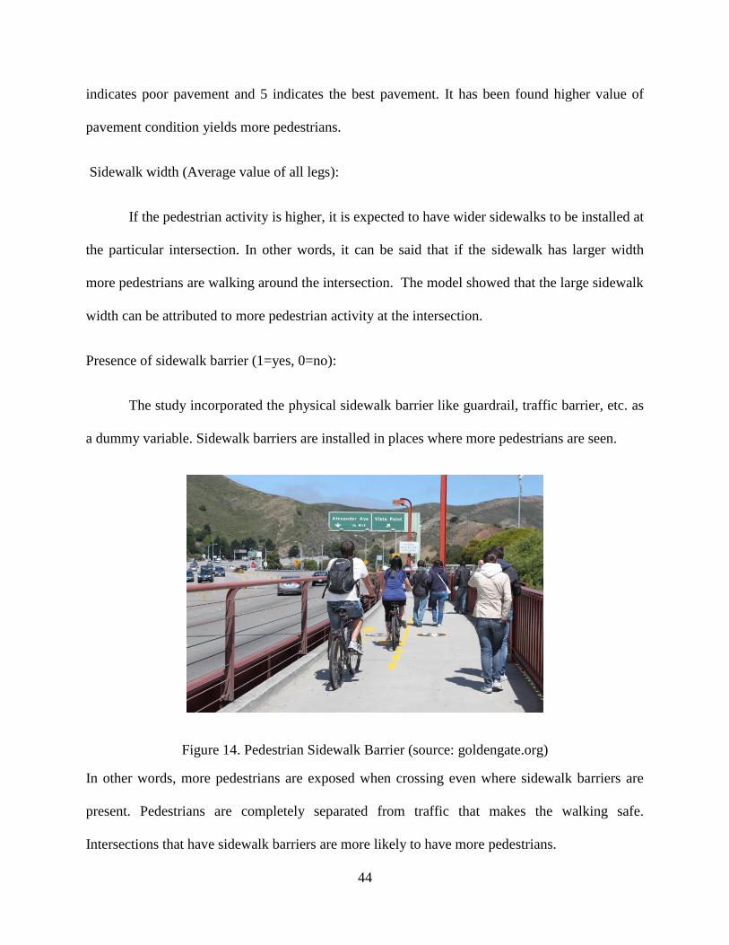
44
indicates poor pavement and 5 indicates the best pavement. It has been found higher value of
pavement condition yields more pedestrians.
Sidewalk width (Average value of all legs):
If the pedestrian activity is higher, it is expected to have wider sidewalks to be installed at
the particular intersection. In other words, it can be said that if the sidewalk has larger width
more pedestrians are walking around the intersection. The model showed that the large sidewalk
width can be attributed to more pedestrian activity at the intersection.
Presence of sidewalk barrier (1=yes, 0=no):
The study incorporated the physical sidewalk barrier like guardrail, traffic barrier, etc. as
a dummy variable. Sidewalk barriers are installed in places where more pedestrians are seen.
Figure 14. Pedestrian Sidewalk Barrier (source: goldengate.org)
In other words, more pedestrians are exposed when crossing even where sidewalk barriers are
present. Pedestrians are completely separated from traffic that makes the walking safe.
Intersections that have sidewalk barriers are more likely to have more pedestrians.

45
Intersection control type (1=signal, 0=stop):
Signalized intersection control type leads to increasing pedestrian activity since it is
relatively safer than the other control types. The study included intersection control type as a
dummy variable and the positive coefficient indicates that if the control type is signal it is more
likely to have higher pedestrian exposure.
5.2 Statistical Test Results Comparing Observed & Predicted Pedestrian Trips
Most of the models identified almost similar significant exposure-related variables that
have been described in the previous section. The predicted pedestrian trips were calculated using
the best exposure model. In order to check the significance of the difference between observed
pedestrian trips and predicted pedestrian trips, both t-test and Wilcoxon signed-rank test were
performed. The results of the tests are shown in Table 6.
Table 6. Statistical test to compare observed and predicted pedestrian trips
Test Statistic p-Value
Student's (t) -1.596 0.1173
Signed Rank (S) -160 0.1013
The results of both tests yielded a p-value greater than 0.05, which indicates there is no
significant difference between the mean of the observed pedestrian trips and the predicted
pedestrian trips. It implies that the predicted pedestrian trips could be used in lieu of the actual
pedestrian trips if there were no pedestrian counts available in the study area.

46
5.3 Results of the Crash Models Developed using Predicted Pedestrian Trips
Using the predicted pedestrian trips from the Tobit model, Negative Binomial and ZINB
crash models were developed. In these models pedestrian trips have been used as exposure to
predict the number of crash at a particular intersection. In order to evaluate how the predicted
pedestrian trips perform relative to observed pedestrian trips, a similar type of crash model was
developed using the original observed pedestrian trips as exposure. The Negative Binomial crash
models are described in Table 7 and Table 8.
Table 7. NB crash model using predicted trips from exposure model
Parameter Estimate Standard
Error
p-value
Intercept -0.962 0.254 0.0002
Predicted Pedestrian Trips 0.0166 0.004 <.0001
Dispersion 0.851 0.276 .
Table 8. NB crash model using original pedestrian trips as exposure
Parameter Estimate Standard Error p-value
Intercept -0.667 0.179 0.0002
Original Pedestrian Trips 0.010 0.002 <.0001
Dispersion 0.728 0.259 .
All the developed models are summarized in Table 9 based on AIC and BIC values.
Table 9 shows that the crash models from observed and predicted pedestrian trips have
almost the same AIC and BIC values for both modeling techniques. It indicates that the predicted
pedestrian trips performed almost the same as the original pedestrian trips in the crash models.
Thus the approach of surrogate measures for pedestrian exposure is justified here. It was also
found that the NB crash model performed slightly better than the ZINB model in terms of AIC

47
and BIC values although the dataset contained almost 66% of intersections with no pedestrian
crashes. In this two-step safety analysis not only the predicted crashes but also the predicted
volume of pedestrian trips can be obtained.
Table 9. Comparison of developed crash models
Negative Binomial (NB) Crash Models AIC BIC
NB using predicted trips from pedestrian exposure model (Tobit
model using all variables)
349.04 357.73
NB using observed pedestrian trips 351.25 359.99
Zero-Inflated Negative Binomial (ZINB) Crash Models AIC BIC
ZINB using predicted trips from pedestrian exposure model (Tobit
model using all variables)
351.04 362.63
ZINB using observed pedestrian trips 352.79 367.28
5.4 Injury Severity Analysis Results
The response profile of the pedestrian injury severity is inherently ordered that lead to the
application of ‘Ordered Logit’ model. The results of the ‘Ordered Logit’ model are summarized
in Table 10, 11, 12. The log likelihood value of the model is 1303.51 which is the smallest
possible value obtained after using different combinations of the explanatory variables. Also
there is a reduction in the log likelihood value with the presence of covariates along with the
intercept. In this analysis a significance level α = 0.05 is taken to define the significant factors.

48
Table 10. Model Fit Statistics of ‘Ordered Logit’ Model
Criterion Intercept Only Intercept & Covariates
Covariates AIC 1526.606 1327.513
SC 1536.175 1384.926
-2 Log L 1522.606 1303.513
Table 11. Significant Explanatory Variables of Injury Severity Analysis
Parameter Estimate Standard
Error
p-value
Intercept -3.112 0.219 <.0001
Intercept -1.081 0.186 <.0001
Intersection Presence (1=yes, 0=No) -0.330 0.154 0.0317
Crash in Local Rd (1=yes, 0=No) -0.895 0.182 <.0001
Alcohol/Drug Involve (1=yes, 0=No) 1.393 0.213 <.0001
Lighted Dark Condition (1=yes, 0=No) 0.515 0.194 0.0079
Unlighted Dark Condition (1=yes, 0=No) 1.026 0.192 <.0001
Pedestrian in a Hurry (1=yes, 0=No) 0.546 0.190 0.0041
Road Speed 40 mph or more (1=yes, 0=No) 0.612 0.171 0.0003
Elder Pedestrian Involve (1=yes, 0=No) 0.766 0.239 0.0013
Table 12. Association of Predicted Probabilities and Observed Response
Percent Concordant 73.8 Somers' D 0.499
Percent Discordant 23.9 Gamma 0.511
Percent Tied 2.3 Tau-a 0.259
Pairs 202531 c 0.750

49
Table 12 shows that 73.8 percentage of pairs where the observation with the desired
outcome (event) has a higher predicted probability than the observation without the outcome
(non-event). The model has a c-statistics (Area under ROC) curve value of 0.75 which indicates
the model performs reasonably well in distinguishing fatal, severe injury and minor injury. The
next section provides a brief explanation of the explanatory variables obtained in Table 11.
Intersection Presence (1=yes, 0=No):
It can be observed from the model that pedestrian injury severity levels tend to have
lower order (possible or minor injury) if there is intersection involvement associated with the
crash. In other words it can be said that the injury severity is higher if the crash location is other
than intersection (midblock, driveway access etc.). The effect can be explained in the way that
when any vehicle approaches the intersection, it usually gets slow down either to follow the
signal/signs or to negotiate the turning movement. Besides the drivers are more careful to yield
the pedestrians at the intersection (Zajac and Ivan, 2003). It results in the reduction of number of
vehicle-pedestrian conflicts at the intersection. On the other hand, the impact of vehicle
pedestrian collision is relatively higher due to high speed and continuous movement for the crash
locations other than intersection. The resulting collision leads to higher injury for such locations.
Crash in Local Rd (1=yes, 0=No):
The functional classification of road system is defined as interstate, freeway, arterial,
collector and local. It is obvious that the presence of pedestrian (so the pedestrian crash) is rare in
interstate and freeway roads. The pedestrian injury severity for the crashes occurring in local
road has lower order relative to other road system. Since the vehicle travelling speed in local
roads is relatively low and the roads are narrow with relatively high volume of traffic, the crash

50
is relatively less severe. The driver pedestrian interaction in local roads is relatively safe than the
other road system since drivers obviously expect the presence of pedestrian. The higher co-
efficient value for the road system variable indicates that the injury is highly severe for the
pedestrian crashes occurring other than local roads.
Alcohol/Drug Involve (1=yes, 0=No):
The model shows that alcohol drug has the highest co-efficient value in magnitude
compared to other variables. It implies that Alcohol drug involvement in crashes is the most
important factor responsible for higher injury severity of pedestrians. Pedestrians under the
influence of drug or alcohol may accidently fall on the roadway from the sidewalk and stuck
with the vehicle heavily since they have less control over their brain.
Figure 15. Alcohol leads to Fatality (source: Mother Jones / NHTSA)
They may be less careful while walking on the road and during night condition the situation get
worsen. Even if the drivers are careful they can hardly do anything if a pedestrian under alcohol
comes suddenly in front of the vehicle. The resulting injury severity is incapacitating or fatal.

51
Lighted Dark Condition (1=yes, 0=No):
Light condition plays a significant role in pedestrian crash severity. During the day it is
easy to see the pedestrian walking or crossing on the road but it becomes hard for the drivers to
screen the pedestrians during the night if they are not wearing any reflective clothes or shoes.
Unless the drivers approach close to the pedestrian even with the presence of street light or other
source of light, they couldn’t realize if there is actually a pedestrian walking.
Unlighted Dark Condition (1=yes, 0=No):
The crashes are more severe if there is no source of light under dark condition. It must be
mentioned that the impact of the unlighted dark condition on injury severity is higher than the
impact of lighted dark condition. The higher value of the co-efficient for the unlighted dark
variable confirms this in the model.
Figure 16. Pedestrian under Dark Condition (Source: Getty Images)
Obviously the situation is worst for the unlighted dark condition to detect the pedestrians. In
Central Florida the majority of the streets are unlighted and the vehicle light is the only source.
But the vehicle light is more focused on directing the roadway direction rather than the

52
pedestrian detection. The resulting pedestrian vehicle collision causes injury severity of higher
order (incapacitating, fatal).
Pedestrian in Hassle:
The injury severity of pedestrian depends a lot on the action of pedestrian during the
crash. If the pedestrians are aware of the surrounding environment there is less chance of a crash.
Even if the crash occurs there is more likely to happen minor injury. The variable pedestrian in
hassle describes that if the pedestrians were in a hurry during the crash occurrence the resulting
injury severity is of higher order. It also shows that the injury severity is higher for pedestrian in
hassle relative to other improper action such as failure to yield right-of-way, failure to obey
traffic signs, signals etc.
Figure 17. Pedestrians walking in a Hurry (source: Inhabitat)
It is obvious that the pedestrian in hassle is less attentive on walking which may cause improper
road crossing, jump off the sidewalk, sudden fall on roadway etc. It indicates that pedestrian in a
hurry may lead to many other action that may results in crash and higher injury severity.

53
Pedestrians are known as vulnerable road users which increase to a higher level of vulnerability
when they rush on road.
Road Speed 40 mph or more (1=yes, 0=No):
Roadway speed limit is a relative measurement of vehicle traveling on road. More often it
is seen that vehicles are travelling at a higher speed than the specified limit of the roadway
section. The variable ‘rdspeed40plus’ shows that there is an increased probability of higher
injury particularly incapacitating and fatal injuries. Waiz et al. (1983) reported that the reduction
of the speed limit from 60 to 50 km/h in Zurich was accompanied by a reduction of 20% in
pedestrian casualties and a 25% decrease in pedestrian fatalities.
Figure 18. Impact of vehicle Speed on Pedestrian Fatality (Source: saferspeedarea.org.nz)
In Central Florida region vehicle with roadway speed limit more than 40 may cause a serious
threat to the safety of people walking on the road.

54
Elder Pedestrian Involve (1=yes, 0=No):
Central Florida has a higher proportion of people aged more than 65. These people may
be reluctant to drive or walk on the road for their commuting. The elder pedestrians exposed to
high speed vehicle are more vulnerable to injury severity. It can be seen from the model that the
crashes where elderly pedestrians are involved results in higher injury severity. The health
condition of elder pedestrian is more vulnerable to higher injury. Moreover the elder pedestrians
while walking on the road are less likely to pay attention of the surrounding environment.
Figure 19. Elder Pedestrian Requires Special Assistant (source: Chip Latherland/NY Times)
5.5 k fold cross validation result
The primary purpose of the ordered logit model is to identify the contributing factors of
higher pedestrian injury severity rather than predicting the injury. Although it is not essential to
validate the model since the data used are the actual crash data but in order to evaluate modeling
performance 10-fold cross validation method was adopted. The k-fold cross validation method

55
calculated the area under ROC curve (c value) for each of the 10 subsets and the average c value
is obtained to see whether it significantly drops from the actual model c statistics that uses all the
training data. The result obtained in the 10-fold cross validation is summarized in Table 13.
Table 13. c Statistics for 10 fold Cross Validation
Optimistic c Optimism Correction Corrected c
0.7517 0.0242 0.7275
The table shows that the average c value of the 10-subset of the original data is 0.72
where the original value of the c statistics is 0.75. The difference is much smaller indicating the
model performed reasonably well in representing pedestrian injury severity.
Table 14. Lift Table Created for Injury Severity Profile
Injury Severity
No=0 Yes=1 Total
Minor Injury =1 125
11.31
575
52.04
700
63.35
Major Injury=2 97
8.78
197
17.83
294
26.61
Fatal=3 80
7.24
31
2.81
111
10.05
Total 302
27.33
803
72.67
1105
100.00
Table 14 shows the lift table for the injury severity profile. It can be seen from the table
that the model can correctly classify 803 observations out of 1105 data sample which indicates
the model performs moderately well in injury severity distinguishing.

56
CHAPTER 6. CONCLUSIONS AND RECOMMENDATIONS
Over the past decades, practitioners have adopted various approaches to develop
knowledge and guidelines for pedestrian safety. Recently, many researchers have focused on
pedestrians’ safety by identifying risk factors. However, depending only on crash counts without
considering the underlying risk factors may provide limited and even biased information about
where safety measures are needed and what measures would be the best to be used to improve
pedestrian safety (Wang et al., 2016).
In the exposure estimation part of this study, a systemic approach has been developed
that uses pedestrian surrogate measures in terms of exposure information. The two-steps
procedure described in the study can be utilized in cases where it is difficult to collect the
pedestrian volume data. The study recommends using the two-steps procedure as it provides
important exposure information to better understand the pedestrian activity and crash frequency
relation. The study applied negative binomial and zero-inflated negative binomial models in
micro-level pedestrian safety analysis and found that the negative binomial model performed
slightly better. Apart from these, the identification of the factors affecting pedestrian exposure
such as the presence of school, car-ownership, pavement condition, sidewalk width, bus
ridership, intersection control type, and presence of sidewalk barrier was another important
contribution of the study to the pedestrian safety research approach. The study emphasizes
focusing on these factors while determining the safety measures for pedestrians. For example, if
there is a school near an intersection, strict enforcement of speeding and traffic calming is
required, and also pedestrian education programs should be promoted for the school children
(Abdel-Aty et al., 2007).

57
There are several possible extensions of this study that could be made in the future. The
proposed two-steps procedure in this study involves two consecutive modeling processes. The
first model estimates the number of pedestrians; and the second model estimates pedestrian crash
counts using the predicted pedestrian counts from the first model. Nevertheless, the procedure
has a limitation as the result can be biased due to the accumulated errors from the first step. It is
possible that the issue can be overcome by adopting simultaneous modeling approach. The
influential area around each intersection (buffer size) considered in the study for extracting
socio-economic and land-use variables was determined based on the average walking distance
(Boer et al., 2007; Yang and Diez-Roux, 2012). However, it is common to have a longer trip
distance than the average walking distance. It may be possible that the variables found to be
insignificant in the current study may become significant using other buffer sizes. The study can
be done using different buffer sizes to identify other significant factors. In such case mixed
models or random variables would be better approach for the analysis.
The injury severity analysis part of the study recognizes the responsible conditions or
factors for severe pedestrian injury severity in Central Florida. Based on the identified
contributing factors it would be helpful to select the appropriate countermeasures to alleviate
pedestrian injury severity of this region. The results may also be useful in the region based
pedestrian safety policy evaluation. However, the study can further be extended in several ways.
More complex modeling techniques such as mixed ordered logit model or random effects model
can be applied to see if the model results remain similar. It is obvious that many of the pedestrian
crashes are not reported to the police. The results obtained in the safety studies are approximate
since there could be more information that is lost due to this unwillingness of crash reporting.
The injury severity study can be further extended including several crash databases specifically

58
combining the safety office crash data and hospital records. The explanatory variables used in
the model can further be combined to identify any other significant factor that may cause severe
pedestrian injury.
Based on the study it is recommended that proper safety measures be taken before the
condition get worse. The following safety measures can be adopted depending on the cost and
desired efficiency to improve pedestrian safety (Table 15).
Infrastructure Measures:
Table 15. Engineering/ITS Based Safety Countermeasures (FHWA, 2014).
Engineering/ITS based Countermeasures Cost Efficiency
Advanced Yield Markings for Motorists Low High
In-roadway Knockdown Signs Low
Pedestrian Countdown Signals with Animated Eyes Medium
Danish Offset High
Median Refuge High
Portable Speed Trailer High
Pedestrian Activated Flashing Yellow High
Pedestrian Call buttons that Confirm Call (Visible/Audible confirmation) Low Medium
Turning Vehicles Yield to Pedestrians Low
ITS No-Turn on Red Signs Medium
ITS Automatic Pedestrian Detection Devices High

59
Engineering/ITS based Countermeasures Cost Efficiency
Warning Signs for Motorists Low Low
High Visibility Crosswalk Treatment Medium
Pedestrian Channelization High
Smart Lighting High
Educational Measures:
Intensifying road safety awareness and publicity campaign including pragmatic measures
to improve and correct road user behaviors through public motivational programs.
Education can help to bring about a climate of concern and develop sympathetic attitudes
towards effective interventions.
Road Safety Education for school children of various age groups.
Enhancing programs of law enforcement with public information and education
campaigns.
Enforcement Measures:
Strong, but fair and targeted, enforcement is critical to the safe and efficient use of road
system. Traffic law enforcement requires professional skills that are different from other
types of police work.
Effective enforcement of laws and sanctions against alcohol/drugs impaired drivers and
to bring about changes in attitudes of drivers towards safe operations.

60
Combined with enforcement, road safety publicity campaigns improve road user behavior
and reduce road accident.
An information briefing, educating police forces about the issue and importance of
specific enforcement measures.
Extensive public information and advertising.
It is expected that the study can be a good platform for further analysis of pedestrian safety
not only at intersections but also on segments with surrounding environments. The injury
severity analysis results and the methodologies implemented in the study including surrogate
exposure variables can estimate reliable safety performance functions for pedestrian crashes even
though pedestrian trip data is not available. With the reliable pedestrian safety performance
functions, it would be possible to identify crash hotspots for pedestrians and provide appropriate
countermeasures to prevent pedestrian crashes.

61
REFERENCES
[1] NHTSA. Traffic Safety Facts: Pedestrian Data, May 2016.
https://crashstats.nhtsa.dot.gov/Api/Public/ViewPublication/812270. Accessed December 16,
2016.
[2] NZTA. Economic Evaluation Manual. http://www.nzta.govt.nz/assets/resources/economic-
evaluation-manual/volume-2/docs/eem2-july-2010.pdf. Accessed February 26,2017.
[3] Rahul, T., and Verma, A. Economic impact of non-motorized transportation in Indian cities.
Research in transportation economics, Vol. 38, No. 1, 2013, pp. 22-34.
[4] Lee, I.-M., and Buchner, D. M. The importance of walking to public health. Medicine and
science in sports and exercise, Vol. 40, No. 7 Suppl, 2008, pp. S512-518.
[5] Raford, N., and Ragland, D. R. Pedestrian volume modeling for traffic safety and exposure
analysis. Safe Transportation Research & Education Center, 2005.
[6] Tobey, H., Knoblauch, R. L., and Shunamen, E. Pedestrian Trip Making Characteristics and
Exposure Measures. Final Report. Federal Highway Administration, Office of Safety and Traffic
Operations, 1983.
[7] Lassarre, S., Papadimitriou, E., Yannis, G., and Golias, J. Measuring accident risk exposure
for pedestrians in different micro-environments. Accident Analysis & Prevention, Vol. 39, No. 6,
2007, pp. 1226-1238.
[8] Davis, D. G., and Braaksma, J. P. Adjusting for luggage-laden pedestrians in airport
terminals. Transportation Research Part A: General, Vol. 22, No. 5, 1988, pp. 375-388.

62
[9] Qin, X., and Ivan, J. Estimating pedestrian exposure prediction model in rural areas.
Transportation Research Record: Journal of the Transportation Research Board, No. 1773,
2001, pp. 89-96.
[10] Lam, W. W., Yao, S., and Loo, B. P. Pedestrian exposure measures: A time-space
framework. Travel Behaviour and Society, Vol. 1, No. 1, 2014, pp. 22-30.
[11] FL-DHSMV. Crash Facts. https://www.flhsmv.gov/resources/crash-citation-reports/.
Accessed December 29, 2016.
[12] T4A. Transportation for America. http://t4america.org/2011/05/27/newspapers-across-the-
country-call-for-increased-pedestrian-safety-following-dangerous-by-design-rankings/. Accessed
07 January 2017.
[13] FHWA. Pedestrian Safety Countermeasures Deployment and Evaluation.
https://safety.fhwa.dot.gov/ped_bike/pssp/background/psafety.cfm. Accessed 24 January, 2017.
[14] Jacobs, P., Klarenbach, S., Ohinmaa, A., Golmohammadi, K., Demeter, S., and
Schopflocher, D. Chronic diseases in Alberta: cost of treatment and investment in prevention.
Citeseer, 2004.
[15] Lee, J., Abdel-Aty, M., Choi, K., and Huang, H. Multi-level hot zone identification for
pedestrian safety. Accident Analysis & Prevention, Vol. 76, 2015, pp. 64-73.
[16] Ukkusuri, S., Hasan, S., and Aziz, H. Random parameter model used to explain effects of
built-environment characteristics on pedestrian crash frequency. Transportation Research
Record: Journal of the Transportation Research Board, No. 2237, 2011, pp. 98-106.

63
[17] Lee, C., and Abdel-Aty, M. Comprehensive analysis of vehicle–pedestrian crashes at
intersections in Florida. Accident Analysis & Prevention, Vol. 37, No. 4, 2005, pp. 775-786.
[18] Keall, M. D. Pedestrian exposure to risk of road accident in New Zealand. Accident Analysis
& Prevention, Vol. 27, No. 5, 1995, pp. 729-740.
[19] Miranda-Moreno, L. F., Morency, P., and El-Geneidy, A. M. The link between built
environment, pedestrian activity and pedestrian–vehicle collision occurrence at signalized
intersections. Accident Analysis & Prevention, Vol. 43, No. 5, 2011, pp. 1624-1634.
[20] Abdel-Aty, M., Chundi, S. S., and Lee, C. Geo-spatial and log-linear analysis of pedestrian
and bicyclist crashes involving school-aged children. Journal of safety research, Vol. 38, No. 5,
2007, pp. 571-579.
[21] Kweon, Y.-J. Development of crash prediction models with individual vehicular data.
Transportation research part C: emerging technologies, Vol. 19, No. 6, 2011, pp. 1353-1363.
[22] Lord, D., Washington, S. P., and Ivan, J. N. Poisson, Poisson-gamma and zero-inflated
regression models of motor vehicle crashes: balancing statistical fit and theory. Accident
Analysis & Prevention, Vol. 37, No. 1, 2005, pp. 35-46.
[23] Lord, D., Washington, S., and Ivan, J. N. Further notes on the application of zero-inflated
models in highway safety. Accident Analysis & Prevention, Vol. 39, No. 1, 2007, pp. 53-57.
[24] Van den Bossche, F., Wets, G., and Brijs, T. Role of exposure in analysis of road accidents:
a Belgian case study. Transportation Research Record: Journal of the Transportation Research
Board, No. 1908, 2005, pp. 96-103.

64
[25] Wier, M., Weintraub, J., Humphreys, E. H., Seto, E., and Bhatia, R. An area-level model of
vehicle-pedestrian injury collisions with implications for land use and transportation planning.
Accident Analysis & Prevention, Vol. 41, No. 1, 2009, pp. 137-145.
[26] Cervero, R. Mixed land-uses and commuting: evidence from the American Housing Survey.
Transportation Research Part A: Policy and Practice, Vol. 30, No. 5, 1996, pp. 361-377.
[27] Graham, D. J., and Stephens, D. A. Decomposing the impact of deprivation on child
pedestrian casualties in England. Accident Analysis & Prevention, Vol. 40, No. 4, 2008, pp.
1351-1364.
[28] Loo, B., and Yao, S. Area deprivation and traffic casualties: the case of Hong Kong.In
Transportation and Urban Sustainability: Proceedings of the 15th International Conference of
Hong Kong Society for Transportation Studies, HKSTS 2010, Hong Kong Society for
Transportation Studies., 2010.
[29] Cai, Q., Lee, J., Eluru, N., and Abdel-Aty, M. Macro-level pedestrian and bicycle crash
analysis: incorporating spatial spillover effects in dual state count models. Accident Analysis &
Prevention, Vol. 93, 2016, pp. 14-22.
[30] Eluru, N., Bhat, C. R., and Hensher, D. A. A mixed generalized ordered response model for
examining pedestrian and bicyclist injury severity level in traffic crashes. Accident Analysis &
Prevention, Vol. 40, No. 3, 2008, pp. 1033-1054.
[31] Mohamed, M. G., Saunier, N., Miranda-Moreno, L. F., and Ukkusuri, S. V. A clustering
regression approach: A comprehensive injury severity analysis of pedestrian–vehicle crashes in
New York, US and Montreal, Canada. Safety science, Vol. 54, 2013, pp. 27-37.

65
[32] Kim, J.-K., Ulfarsson, G. F., Shankar, V. N., and Mannering, F. L. A note on modeling
pedestrian-injury severity in motor-vehicle crashes with the mixed logit model. Accident
Analysis & Prevention, Vol. 42, No. 6, 2010, pp. 1751-1758.
[33] Pour-Rouholamin, M., and Zhou, H. Investigating the risk factors associated with pedestrian
injury severity in Illinois. Journal of safety research, Vol. 57, 2016, pp. 9-17.
[34] Train, K. E. Discrete choice methods with simulation. Cambridge university press, 2009.
[35] Quddus, M. A., Wang, C., and Ison, S. G. Road traffic congestion and crash severity:
econometric analysis using ordered response models. Journal of Transportation Engineering,
Vol. 136, No. 5, 2009, pp. 424-435.
[36] Abdel-Aty, M. Analysis of driver injury severity levels at multiple locations using ordered
probit models. Journal of safety research, Vol. 34, No. 5, 2003, pp. 597-603.
[37] Eluru, N., and Bhat, C. R. A joint econometric analysis of seat belt use and crash-related
injury severity. Accident Analysis & Prevention, Vol. 39, No. 5, 2007, pp. 1037-1049.
[38] Wang, X., and Abdel-Aty, M. Analysis of left-turn crash injury severity by conflicting
pattern using partial proportional odds models. Accident Analysis & Prevention, Vol. 40, No. 5,
2008, pp. 1674-1682.
[39] Zhu, X., and Srinivasan, S. A comprehensive analysis of factors influencing the injury
severity of large-truck crashes. Accident Analysis & Prevention, Vol. 43, No. 1, 2011, pp. 49-57.
[40] Glosup, J. Generalized linear models: An applied approach.In, Taylor & Francis, 2005.
66
[41] McCullagh, P. Generalized linear models. European Journal of Operational Research, Vol.
16, No. 3, 1984, pp. 285-292.
[42] Washington, S. P., Karlaftis, M. G., and Mannering, F. Statistical and econometric methods
for transportation data analysis. CRC press, 2010.
[43] Breiman, L. Random forests. Machine learning, Vol. 45, No. 1, 2001, pp. 5-32.
[44] Woolson, R. Wilcoxon Signed‐Rank Test. Wiley Encyclopedia of Clinical Trials, 2008.
[45] Lord, D., and Mannering, F. The statistical analysis of crash-frequency data: a review and
assessment of methodological alternatives. Transportation Research Part A: Policy and
Practice, Vol. 44, No. 5, 2010, pp. 291-305.
[46] Rose, C. E., Martin, S. W., Wannemuehler, K. A., and Plikaytis, B. D. On the use of zero-
inflated and hurdle models for modeling vaccine adverse event count data. Journal of
biopharmaceutical statistics, Vol. 16, No. 4, 2006, pp. 463-481.
[47] Lambert, D. Zero-inflated Poisson regression, with an application to defects in
manufacturing. Technometrics, Vol. 34, No. 1, 1992, pp. 1-14.
[48] Williams, R. Generalized ordered logit/partial proportional odds models for ordinal
dependent variables. Stata Journal, Vol. 6, No. 1, 2006, p. 58.
[49] James, G., Witten, D., Hastie, T., and Tibshirani, R. An introduction to statistical learning.
Springer, 2013.

67
[50] Boer, R., Zheng, Y., Overton, A., Ridgeway, G. K., and Cohen, D. A. Neighborhood design
and walking trips in ten US metropolitan areas. American journal of preventive medicine, Vol.
32, No. 4, 2007, pp. 298-304.
[51] Yang, Y., and Diez-Roux, A. V. Walking distance by trip purpose and population
subgroups. American journal of preventive medicine, Vol. 43, No. 1, 2012, pp. 11-19.
[52] Zajac, S. S., and Ivan, J. N. Factors influencing injury severity of motor vehicle–crossing
pedestrian crashes in rural Connecticut. Accident Analysis & Prevention, Vol. 35, No. 3, 2003,
pp. 369-379.
[53] Waiz, F. H., Hoefliger, M., and Fehlmann, W. Speed limit reduction from 60 to 50 km/h and
pedestrian injuries.In, SAE Technical Paper, 1983.
[54] Wang, Y., Sharda, S., and Wang, H. A Systemic Safety Analysis of Pedestrian Crashes:
Lessons Learned.In Transportation Research Board 95th Annual Meeting Compendium of
Papers, 2016.