1

Peer Pressure in Corporate Earnings Management*

Constantin Charles, Markus Schmid#, and Felix von Meyerinck

Swiss Institute of Banking and Finance, University of St. Gallen, CH-9000 St. Gallen, Switzerland

This Version: June 2017

Preliminary first draft: Please do not cite without the authors’ consent

Abstract

We show that peer firms play an important role in shaping corporate earnings management de-

cisions. To overcome identification issues in isolating peer effects, we use fund flow-induced

selling pressure by passive open-end equity mutual funds as exogenous shocks to firms’ stock

prices. Managers respond to such exogenous price shocks by adjusting earnings management

policies. We then measure individual firms’ reactions to changes in earnings management at

peer firms as a result of such exogenous price shocks. The documented peer effect in earnings

management is not only statistically, but also economically significant. Our results are robust to

alternative measures of fund flow-induced selling pressure and earnings management, and to

estimating instrumental variables regressions in which we instrument peer firms’ earnings man-

agement with mutual fund flow-induced selling pressure.

JEL Classification: G32, L14

Keywords: Peer effects; Earnings reporting; Discretionary accruals; Mutual fund flows; Price pressure

_____________________________

* We are grateful to Martin Brown, John Chalmers, Jasmin Gider, Andreas Kaeck, and Naciye Sekerci,

conference participants at the 2017 annual conference of the Swiss Society for Financial Market Research

(SGF) in Zurich and the 2017 French Finance Association (AFFI) conference in Valence, and seminar par-

ticipants at Technical University of Munich, University of St. Gallen, and University of Sussex for helpful

comments and discussions. Part of this research was completed while Schmid and von Meyerinck were

visiting Stern School of Business at New York University. Corresponding author: Tel.: +41-71-224-7042; E-mail: markus.schmid@unisg.ch.

Address: Swiss Institute of Banking and Finance, University of St. Gallen, 9000 St. Gallen, Switzerland.

2

1. Introduction

Corporate earnings are an important source of information not only for company sharehold-

ers, but also for a broader audience, including competitors, other investors, analysts, and regulators.

Yet managers have a certain degree of discretion over reported earnings. They can (and do) affect

the informativeness of earnings and the transparency of financial reporting by engaging in earnings

management. While there is a large literature on within-firm and firm-specific monitoring-related

determinants of earnings management1, managers might change earnings management policies just

because other managers do so as well. The existence of peer effects in earnings management would

thus imply that the transparency and earnings quality of entire industries improves or deteriorates

simply because certain companies in the industry change their earnings management policies, ef-

fectively leading others to follow suit.

There are several reasons why we expect to find peer effects in corporate earnings manage-

ment. First, for an individual firm, the optimal (and acceptable) amount of earnings management

is difficult to determine. Hence, firms might rationally resort to copying their peers, consistent with

the literature on herding (e.g., Banerjee, 1992) and the literature on informational cascades (e.g.,

Bikhchandani, Hirshleifer, and Welch, 1992). Second, firms are compared to their peers on a reg-

ular basis and compete for investor, analyst, and general public goodwill and recognition. Consist-

ently, Hameed, Morck, Shen, and Yeung (2015) show that analysts are disproportionally more

likely to follow firms with fundamentals that correlate more with those of their industry peers.

Muslu, Rebello, and Xu (2014) document significant return comovement of stocks covered by the

same analysts. Thus, an individual firm’s desirable (and acceptable) level of earnings management

is likely to depend on the earnings management of other firms in its peer group. Indeed, in a recent

1 See DeAngelo (1981); Watts and Zimmerman (1986); DeFond and Park (1997); Nissim and Penman (2001); Leuz,

Nanda, and Wysocki (2003); Irani and Oesch (2016).

3

survey of 169 CFOs, Dichev, Graham, Harvey, and Rajgopal (2013) show that CFOs themselves

state that peer comparisons are one of the most useful red flags in detecting earnings management

at individual firms. Finally, managers are evaluated against peer firm managers by internal as well

as external parties. Most importantly, managerial compensation is often based on financial perfor-

mance measures relative to a peer group (Aggarwal and Samwick, 1999; Antón, Ederer, Giné, and

Schmalz, 2016). Furthermore, theoretical (Zwiebel, 1995) and empirical (Jenter and Kanaan, 2015)

research suggests that managerial turnover depends on performance relative to a peer group. Hence,

managers may engage in earnings management out of reputational, compensation, and career con-

cerns if managers at peer firms do so as well.

Identifying peer effects in corporate earnings management is empirically challenging as earn-

ings management is an endogenous choice variable. Moreover, we face an identification challenge

that is common to nearly all papers on peer effects. This challenge comes from a special type of

endogeneity referred to as the “reflection problem” (Manski, 1993; Leary and Roberts, 2014). The

concern is that there might be a self-selection of firms into peer groups. In the context of our study,

shared unobservable characteristics or preferences of peer group members might determine earn-

ings management of all members of the peer group, and thus lead to a correlation of earnings man-

agement within a peer group. To overcome this identification problem, we need an exogenous

event that affects earnings management at one firm in the peer group, but does not directly affect

earnings management at other firms within the peer group. We use fund flow-induced selling pres-

sure by passive (i.e., equity index) mutual funds as an exogenous shock to stock prices (e.g., Coval

and Stafford, 2007; Khan, Kogan, and Serafeim, 2012). We first empirically show that such shocks

have an economically and statistically significant effect on the affected firms’ stock returns. For

individual firms, these shocks come as a surprise since the selling of shares by passive mutual funds

is not driven by firm fundamentals, but by liquidity needs of passive fund investors. Managers

4

respond to such exogenous price shocks by reducing earnings management, which we measure

with discretionary accruals from the modified Jones model (Dechow, Sloan, and Sweeney, 1995).

An explanation for this finding is that monitoring by the board, analysts, investors, and short sellers

increases following the sudden price shock. In response to the increased scrutiny, managers reduce

earnings management.2 Models such as the one proposed by Fishman and Hagerty (1992) suggest

that market prices of company stock help to guide managerial decision making. It follows that

changes in the market price of company stock have real effects since managers respond by recon-

sidering their operating and financing policies (Khan, Kogan, and Serafeim, 2012). Our findings

are thus consistent with the idea that managers respond to increased price pressure by revising their

earnings management policies.

While fund flow-induced selling pressure triggers a reduction in discretionary accruals at the

firm experiencing fund flow-induced selling pressure, it is unlikely to directly affect discretionary

accruals at other firms in the peer group. Our firm-level measure of mutual fund flow-induced

selling pressure is caused by simultaneous outflows at many different passive mutual funds. We

exclusively rely on passive mutual funds to ensure that these flows are not driven by investor pref-

erences for individual firms, but rather by liquidity needs of investors. As assets under management

fluctuate, passive fund managers buy and sell shares with constant portfolio weights, in order to

minimize the tracking error of the fund. Consequently, our measure of fund flow-induced price

pressure is unlikely to be related to individual firm fundamentals, even less so to peer firm funda-

mentals.

2 Analyzing the effect of (exogenous) variation in the threat of short selling, Grullon, Michenaud, and Weston (2015)

find that short selling leads to negative abnormal returns. Using the same setting, Massa, Zhang, and Zhang (2015) and

Fang, Huang, and Karpoff (2016) both find evidence for a disciplining effect of short selling on earnings management.

5

To eventually analyze whether firms adapt their earnings management to the earnings man-

agement of peer firms, we need to identify a firm’s peer group. To this end, we rely on the text-

based network industry classifications (TNIC) of Hoberg and Phillips (2016). These industry clas-

sifications use textual analysis to measure similarity of products mentioned in the product descrip-

tions provided by firms in their 10-K filings and have been shown to be superior to simple and

static industry classifications such as the Standard Industry Classification (SIC) scheme. In fact,

recent papers on corporate peer effects also rely on TNIC to define peer groups (Foucault and

Fresard, 2014; Cao, Liang, Zhan, 2016). We then regress a firm’s discretionary accruals in a given

year on the fraction of peer firms that experience selling pressure, controlling for average peer firm

characteristics, selling pressure at the sample firm, sample firm characteristics, and year and firm

fixed effects. Our results suggest that a larger fraction of peer firms experiencing selling pressure

triggers a significant reduction in discretionary accruals at our sample firms. This result is not only

statistically, but also economically significant. A one standard deviation increase in the fraction of

peer firms experiencing fund flow-induced selling pressure is associated with a decrease in discre-

tionary accruals by about 20% of mean discretionary accruals. We also estimate instrumental var-

iables (IV) regressions in which we instrument peer firms’ discretionary accruals with the fraction

of peer firms that experience selling pressure. The advantage of this setting is that we can directly

assess to which extent firms react to their peers’ actions as opposed to their peers’ characteristics.

In the previously mentioned setting, it is not possible to disentangle the two effects as the coeffi-

cient captures both. The coefficient on instrumented peer firm discretionary accruals is positive and

highly significant, suggesting that firms respond to changes in earnings management of their peers

by changing their earnings management in the same direction. The economic magnitude of this

peer effect is sizeable: a one standard deviation change in peer firms’ (instrumented) discretionary

6

accruals is associated with a change in discretionary accruals at individual firms of approximately

18-21% of the unconditional mean discretionary accruals.

One concern of our analyses is that sample firms may experience fund flow-induced selling

pressure themselves, and hence our identified change in earnings management could be a first-

order effect of a stock price shock rather than a peer effect. To mitigate this concern, we drop all

firms that experience contemporaneous or lagged selling pressure and find similar results. In fur-

ther tests, we use alternative measures of mutual fund flow-induced selling pressure, alternative

peer group definitions based on three-digit SIC industries, and alternative measures of earnings

management, including the Jones (1991) model, the modified Dechow-Dichev model (McNichols,

2004) augmented with firm fixed effects (Lee and Masulis, 2009), and the discretionary revenue

model of Stubben (2010). In all these robustness checks, we continue to find that individual firms

follow their peer firms’ earnings management policies. Finally, we show that firms are especially

sensitive to changes in earnings management of large, profitable, and geographically close peers.

These findings are consistent with the notion that certain firms within a peer group play a more

important role in shaping earnings management policies at individual firms.

Our study contributes to three different streams of research. First, we contribute to the liter-

ature on corporate peer effects. A growing body of research aims at identifying the role that peer

effects play for firm value and corporate policies. Cohen and Frazzini (2008) show that stock re-

turns predict returns of economically linked firms. Hsu, Reed, and Rocholl (2010) find that Initial

Public Offerings are associated with negative stock price effects and a deterioration of future op-

erating performance at the peer firms. Servaes and Tamayo (2014) show that leveraged buyouts

lead to reduced capital spending, free cash flows, and cash holdings and at the same time increased

7

leverage, payout, and more takeover defenses at industry peers. Kaustia and Rantala (2015) docu-

ment that companies are more likely to split their stocks if peer firms have done so recently. Cao,

Liang, and Zhan (2016) show that firms react to their peers’ commitment to undertake corporate

social responsibility policies by adopting similar policies. Gleason, Jenkins, and Johnson (2008)

show that earnings restatements lead to significant share price declines at peer firms. Fracassi

(2016) and Shue (2013) find that CEOs with close ties are more likely to adopt similar operating

and financing policies. Leary and Roberts (2014) show that firms’ financing decisions are re-

sponses to financing decisions and characteristics of peer firms. Peer effects have also been docu-

mented to influence the structure of executive compensation contracts (Bizjak, Lemmon, and

Naveen, 2008; Bizjak, Lemmon, and Ngyuen, 2011). Our paper contributes to the corporate peer

effects literature by showing that peer firms shape individual firms’ earnings management deci-

sions, a previously undocumented domain.

Second, we contribute to the vast literature on the determinants of earnings management,

which has found a substantial number of factors to be correlated with earnings management.

Among them are operating and financial characteristics of a firm (e.g., Watts and Zimmerman,

1986; DeFond and Park, 1997; Nissim and Penman, 2001), audit quality (e.g., DeAngelo, 1981),

as well as external monitoring by financial analysts and short sellers (e.g., Massa, Zhang, and

Zhang, 2015; Fang, Huang, and Karpoff, 2016; Irani and Oesch, 2016) and investor protection

(e.g., Leuz, Nanda, and Wysocki, 2003).3 Our paper contributes to this literature by providing am-

ple evidence that peer firms’ earnings management policies are an important determinant of indi-

vidual firm’s earnings management policies. Moreover, we provide evidence that larger peers,

3 For an overview of the earnings management literature see Healy and Wahlen (1999) and Dechow, Ge, and Schrand

(2010).

8

more profitable peers, and geographically close peers play a more pronounced role in shaping a

firm’s earnings management decisions.

Finally, we contribute to the literature on mutual fund flow-induced price pressure. Coval

and Stafford (2007) propose mutual fund flow-induced selling pressure as a measure to identify

short-term misvaluations of stocks; they show that investors who trade against constrained mutual

funds earn significant returns for providing liquidity. Khan, Kogan, and Serafeim (2012) use pur-

chase price pressure induced by mutual fund inflows to identify short-term stock overvaluations.

They argue that managers can identify and actively exploit deviations of share prices from the

fundamental value since the probability for Seasoned Equity Offerings, insider selling transactions,

and stock-based acquisitions increase following positive price pressure. Edmans, Goldstein, and

Jiang (2012) look at mutual fund selling pressure and find that companies are more likely to become

a takeover target when subject to selling pressure. More recently, Henning, Oesch, and Schmid

(2016) use mutual fund selling pressure to identify whether stock valuations influence the issuance

of company news and find that managers hold back negative news in response to mutual fund-

induced selling pressure. We contribute to this literature by documenting that managers respond to

negative stock price shocks by reducing earnings management and thereby increasing transparency.

To the best of our knowledge, we are also the first paper to use mutual fund flow-induced selling

pressure to identify peer effects. Finally, in the construction of our selling pressure measures, we

focus on flows in and out of passive funds only which are naturally not driven by firm fundamen-

tals.

The remainder of the paper is structured as follows. In Section 2, we describe the data, vari-

ables, and construction of our sample. Section 3 reports our analysis of peer effects in corporate

earnings management. Section 4 concludes.

9

2. Sample Selection, Data, and Variables

In this section, we first outline the estimation of the selling pressure and earnings manage-

ment measures that we use throughout the remainder of the paper. Then we detail the construction

of the sample and the selection of peer groups. Lastly, we discuss sample characteristics.

2.1 Measures of passive mutual fund selling pressure

Coval and Stafford (2007) show that transactions of mutual funds caused by capital flows in

and out of the funds result in institutional price pressure if a substantial fraction of the securities

are simultaneously sold or acquired by mutual funds. Subsequent papers have used mutual fund

flow-induced price pressure to identify ex-post misvaluations of stocks resulting from a short-lived

mismatch of demand and supply of shares (e.g., Edmans, Goldstein, and Jiang, 2012; Khan, Kogan,

and Serafeim, 2012).

These papers implicitly assume that all funds scale their portfolio holdings following capital

in- or outflows, thereby maintaining constant portfolio weights. In reality, however, this assump-

tion may not hold for all funds. Fund managers might selectively adjust fund holdings following a

sudden shock to fund flows and the resulting fund holdings might therefore reflect a preference for

certain investments. It follows that results of previous research might be driven by mutual fund

managers’ preferences for firms with certain fundamental characteristics.

We address this problem by solely relying on changes in holdings of passive mutual funds

for the construction of our measures of fund flow-induced selling pressure. While maintaining the

desirable properties of this measure, the limitation to passive funds comes with several advantages.

First, passive equity mutual funds control significant amounts of capital and invest into a wide

array of firms. Thereby, our restriction to this group of funds still allows a substantial number of

10

firms to experience fund flow-induced price pressure. Second, passive fund flows are unlikely to

be driven by investor appetite for the fundamentals of individual firms held by a fund. Arguably,

fund flows in and out of passive investment vehicles are driven by capital needs of investors or by

the performance of the overall market. Moreover, an investor willing to trade on firm fundamentals

will trade in individual securities directly and not via a fund (much less a passive fund). Third,

passive fund flows are unlikely to be driven by fund manager preferences for firms with certain

fundamentals. Passive fund managers attempt to minimize costs and the tracking error relative to

a benchmark rather than attempt to maximize total return. In contrast to actively managed funds,

buying and selling decisions of passive funds are thus triggered by funds’ in- and outflows and not

by fundamentals of the firms in which the funds are invested. Fourth, managers of passive funds

do not directly engage in monitoring of their holding companies (Dyck, Morse, and Zingales,

2010). Using passive funds to estimate mutual fund flow-induced selling pressure therefore helps

us to rule out a direct monitoring channel as an explanation for our results.4

We closely follow Coval and Stafford (2007) and Khan, Kogan, and Serafeim (2012) in the

construction of our measures of mutual fund flow-induced selling pressure with the exception that

we only use passive mutual funds. As a starting point, we gather data on all open-end US equity

funds contained in the mutual fund database of the Center for Research in Security Prices (CRSP).

We then identify passive funds as funds that are either classified as Exchange Traded Funds (ETFs)

or as index funds in the CRSP mutual fund database. Similar to Chang, Solomon, and Westerfield

(2016), we further classify funds as passive if the fund name contains variations of “Index Fund”,

“Idx Fund”, “ETF”, “S&P 500”, or “NASDAQ 100”.

4 Note that we find negative stock price shocks to be associated with reductions in earnings management. Hence, a

reduction in monitoring associated with fund managers decreasing their stakes in a firm is expected to result in deteri-

oration of reporting quality (i.e., more earnings management) and hence goes against our results.

11

The construction of the passive fund flow-induced price pressure measure requires data on

fund in- and outflows and data on changes in fund holdings. We start by estimating in- and outflows

for our sample of passive funds using data from the CRSP mutual fund database, which allows us

to infer fund flows on a monthly level. Specifically, fund j’s flow in month s is defined as

𝐹𝑙𝑜𝑤𝑗,𝑠 = {𝑇𝑁𝐴𝑗,𝑠 − 𝑇𝑁𝐴𝑗,𝑠−1 ∗ (1 + 𝑅𝑗,𝑠)}/𝑇𝑁𝐴𝑗,𝑠−1 (1)

where 𝑇𝑁𝐴𝑗,𝑠 is fund j’s total net assets in month s and 𝑅𝑗,𝑠 is fund j’s return from month s-1 to

month s. Intuitively, the in- or outflow of a fund in a month is the change in total net assets that is

not due to the return on investment of the fund’s aggregate holdings over the previous month. We

estimate quarterly flows as the sum of monthly flows, since funds file granular holding data only

on a quarterly level with the SEC.

For each resulting fund-quarter observation, we obtain data on a fund’s quarterly holdings

from Thomson Financial. At this stage we follow Lou (2012), who constructs a sample similar to

ours, and impose several restrictions to ensure satisfactory data quality. First, we exclude all funds

that report an investment objective code indicating “international”, “municipal bonds”, “bond &

preferred”, or “metals” in Thomson Financial. Second, we require the aggregate value of equity

holdings of a fund in a quarter in Thomson Financial to be within the range of 75% and 120% of

the fund’s total net assets reported in Thomson Financial.5 Third, total net assets reported in Thom-

son Financial for a fund in a given quarter may not differ by more than a factor of two from those

reported in the CRSP mutual fund database. Fourth, all fund-quarters with total net assets of less

than $1 million in either the Thomson Financial or the CRSP mutual fund database are excluded.

5 This requirement also mitigates concerns that our sample includes synthetic passive mutual funds. Synthetic funds

do not induce any trading pressure in the underlying stocks in response to significant in- or outflows as they replicate

the stock index return by holding equity index futures contracts and bonds.

12

For the remaining observations, we cross-check the data on fund-quarter-holding level with data

from the CRSP daily stock file as of the holding’s reporting date. Specifically, we require that the

share price and the number of shares outstanding reported in Thomson Financial do not differ by

more than 30% from those reported in CRSP. Finally, shares held by a single fund in a given firm

may not exceed the total number of shares outstanding in CRSP. The resulting sample contains

quarterly fund flows as well the corresponding holding positions for each fund-quarter, which are

the necessary inputs to calculate our two continuous trading pressure measures.

Pressure_CS is equivalent to PRESSURE_1 used in Coval and Stafford (2007) and Pres-

sure_KKS is equivalent to the pressure measure used in Khan, Kogan, and Serafeim (2012), with

the difference that we only rely on passive mutual funds to construct both measures. Specifically,

Pressure_CS is defined for firm i in quarter t as:

𝑃𝑟𝑒𝑠𝑠𝑢𝑟𝑒_𝐶𝑆𝑖,𝑡

={∑ (max (0, 𝛥𝐻𝑜𝑙𝑑𝑖𝑛𝑔𝑠𝑗,𝑖,𝑡|𝐹𝑙𝑜𝑤𝑗,𝑡 > 𝑃𝑒𝑟𝑐𝑒𝑛𝑡𝑖𝑙𝑒(90𝑡ℎ)) − 𝑗 ∑ (max (0, −𝛥𝐻𝑜𝑙𝑑𝑖𝑛𝑔𝑠𝑗,𝑖,𝑡|𝐹𝑙𝑜𝑤𝑗,𝑡 < 𝑃𝑒𝑟𝑐𝑒𝑛𝑡𝑖𝑙𝑒(10𝑡ℎ))𝑗 }

𝐴𝑣𝑔𝑉𝑜𝑙𝑢𝑚𝑒𝑖,𝑡−2:𝑡−1 (2)

where 𝛥𝐻𝑜𝑙𝑑𝑖𝑛𝑔𝑠𝑗,𝑖,𝑡 is fund j’s change in shares held of firm i from quarter t-1 to t. Percentiles of

fund flows are calculated across all funds for every quarter separately. 𝐴𝑣𝑔 𝑉𝑜𝑙𝑢𝑚𝑒𝑖,𝑡−2:𝑡−1 is firm

i’s average trading volume of quarters t-2 and t-1. Pressure_KKS is defined similarly:

𝑃𝑟𝑒𝑠𝑠𝑢𝑟𝑒_𝐾𝐾𝑆𝑖,𝑡

={∑ (max (0, 𝛥𝐻𝑜𝑙𝑑𝑖𝑛𝑔𝑠𝑗,𝑖,𝑡|𝐹𝑙𝑜𝑤𝑗,𝑡 > 𝑃𝑒𝑟𝑐𝑒𝑛𝑡𝑖𝑙𝑒(90𝑡ℎ)) − 𝑗 ∑ (max (0, −𝛥𝐻𝑜𝑙𝑑𝑖𝑛𝑔𝑠𝑗,𝑖,𝑡|𝐹𝑙𝑜𝑤𝑗,𝑡 < 𝑃𝑒𝑟𝑐𝑒𝑛𝑡𝑖𝑙𝑒(10𝑡ℎ))𝑗 }

𝑆ℎ𝑎𝑟𝑒𝑠 𝑂𝑢𝑡𝑠𝑡𝑎𝑛𝑑𝑖𝑛𝑔𝑖,𝑡−1(3)

13

where the numerator is identical to that of Pressure_CS and the denominator is firm i’s shares

outstanding in quarter t-1. Intuitively, Pressure_CS and Pressure_KKS both measure the mismatch

of demand and supply of firm i’s shares by funds with extreme flows. If funds with large inflows

buy shares of firm i and funds with large outflows do not sell these shares, the measures are positive

and indicate buying pressure. In contrast, if funds with large outflows sell shares of firm i and funds

with large inflows do not buy these shares, the measures are negative and indicate selling pressure.

Throughout the paper, we report results based on both the Coval and Stafford (2007) and the Khan,

Kogan, and Serafeim (2012) measures.

We also construct UPressure, which is an “unforced” trading pressure measure following

Khan, Kogan, and Serafeim (2012):

𝑈𝑃𝑟𝑒𝑠𝑠𝑢𝑟𝑒𝑖,𝑡 =∑ (𝛥𝐻𝑜𝑙𝑑𝑖𝑛𝑔𝑠𝑗,𝑖,𝑡|𝑃𝑒𝑟𝑐𝑒𝑛𝑡𝑖𝑙𝑒(10𝑡ℎ) ≤ 𝐹𝑙𝑜𝑤𝑗,𝑡 ≤ 𝑃𝑒𝑟𝑐𝑒𝑛𝑡𝑖𝑙𝑒(90𝑡ℎ))𝑗

𝑆ℎ𝑎𝑟𝑒𝑠 𝑂𝑢𝑡𝑠𝑡𝑎𝑛𝑑𝑖𝑛𝑔𝑖,𝑡−1

(4)

This measure captures the net buying/selling of firm i’s shares across all passive funds that

experience neither large inflows nor large outflows. For each quarter, we calculate the deciles of

Pressure_CS, Pressure_KKS, and UPressure. Our exclusive use of passive funds already mitigates

concerns that changes in the holdings of any fund are associated with firm fundamentals. To further

address these concerns, we only define a firm-quarter as a quarter with selling pressure if Pres-

sure_CS (or alternatively, Pressure_KKS) is in the lowest decile and UPressure is in one of the

four middle deciles (4, 5, 6, or 7). This ensures that we do not classify firm-quarters as selling

pressure quarters if there is net selling across all funds in our sample, since this might indicate

14

information-driven selling.6 Variable definitions of these and all other variables used throughout

the study can be found in Table A.1 in the appendix.

2.2 Does mutual fund flow-induced selling pressure affect stock returns?

The sample, which we use throughout the paper, is the result of a three-way merge between

Compustat, CRSP, and our mutual fund selling pressure data. The latter comes in firm-quarter

observations and is available from Q1 2000 to Q4 2014. Depending on the analysis, it is supple-

mented with annual variables from Compustat or quarterly control variables from Compustat and

quarterly stock return data from CRSP. We relegate a detailed sample selection description of the

firm-year panel used in the peer analysis to Section 2.4, and show variable definitions and descrip-

tive statistics of the quarterly sample in the appendix (Tables A.1 and A.2).

In this sub-section, we test whether sell-offs of passive mutual funds trigger drops in stock

prices at the firms experiencing flow-induced selling pressure. Previous papers have already doc-

umented such a relationship (Coval and Stafford, 2007; Edmans, Goldstein, and Jiang, 2012), but

as we deviate from prior research by relying on passive mutual funds only in the estimation of

mutual fund selling pressure, we attempt to confirm such a relationship in our sample. Preliminary

evidence on the relation between passive mutual fund flow-induced selling pressure and quarterly

stock returns is provided in Figure 1. It displays the cumulative average abnormal returns starting

three quarters before the pressure quarter for firms that experience only one quarter with fund flow-

induced selling pressure during our sample period.7 The figure shows that our measure of passive

6 We check whether selling pressure clusters in certain sub-periods of our sample (e.g., the financial crisis of 2007-

2009) or whether it follows certain seasonal patterns. We find this not to be the case. Figure A.1 in the appendix shows

the distribution of selling pressure over our sample period. 7 We only include firms that experience exactly one quarter of selling pressure to ensure that the documented effect in

the figure is not confounded by other shocks and that it is not driven by a small subsample of firms that experience

selling pressure frequently.

15

mutual fund selling pressure is associated with negative abnormal returns in the event quarter

(t = 0). The cumulative abnormal return drops from about 0% in quarter t = -1 to -4% in t = 0

(statistically significant at the 1% level). The quarters following the pressure quarter also exhibit

negative abnormal returns, albeit on a statistically and economically lower level.

We also test whether the relation between selling pressure of passive funds and abnormal

quarterly returns holds up in a multivariate setting, but for brevity we only present these results in

the appendix. We estimate OLS regressions of quarterly abnormal returns on a dummy variable

whether a firm experiences passive mutual fund selling pressure in a quarter, lagged firm charac-

teristics (the natural logarithm of market capitalization, the market to book ratio, ROA, leverage,

and the lagged abnormal return), as well as time and firm fixed effects. Quarterly abnormal returns

are estimated by subtracting the mean quarterly return of the universe of firms held by passive

mutual funds in our sample from the quarterly return of a firm. Alternatively, we adjust a firm’s

quarterly return by subtracting either the CRSP equally weighted return (including distributions)

or the CRSP value weighted return (including distributions). For each firm-quarter, we construct a

firm’s market capitalization from CRSP as a proxy for firm size, the market to book ratio as a proxy

for growth opportunities, ROA as a profitability measure, and book leverage as a measure of capital

structure. Data to construct all these variables comes from the Compustat quarterly and CRSP daily

datasets. Throughout the paper, we winsorize all non-logarithmized variables at the 1% and 99%

level and cluster standard errors at the firm level. The summary statistics of this quarterly return

sample are presented in Table A.2 in the appendix. Most importantly, all three mean abnormal

quarterly sample returns are close to zero and around 4.3% of all firm-quarters in our sample are

quarters with mutual fund selling pressure.

Regression results are reported in appendix Table A.3. We report results for all three alter-

native quarterly abnormal returns. In Columns 1 and 2, we obtain excess returns by subtracting the

16

mean quarterly return of the universe of firms held by passive mutual funds in our sample in that

quarter, in Columns 3 and 4 by subtracting the CRSP equally weighted return including distribu-

tions, and in Columns 5 and 6, by subtracting the CRSP value weighted return including distribu-

tions from the firm’s quarterly return. Columns 1, 3, and 5 report results based on Pressure_CS

and Columns 2, 4, and 6 based on Pressure_KKS. The results across all six columns confirm that

our measure of passive mutual fund-selling pressure is associated with negative and significant

abnormal stock returns. Moreover, selling pressure of passive mutual funds has a sizable impact

on the market value of equity, indicating a quarterly change that ranges from about -0.9% to -1.2%

in this multivariate setting.

2.3 Measures of earnings management

In order to measure the extent of earnings management, we estimate the discretionary portion

of accruals, as is common in the literature (e.g., Massa, Zhang, and Zhang, 2015; Fang, Huang, and

Karpoff, 2016). Our primary measure of earnings management are discretionary accruals from the

modified Jones model (Dechow, Sloan, and Sweeney, 1995). We start by estimating the non-dis-

cretionary (expected) amount of accruals for each firm-year. To do so, we run the following re-

gression for the universe of firms in Compustat in every fiscal year t for every Fama-French 48

industry with at least 20 firms in fiscal years t-4 through t:

𝑇𝑜𝑡𝑎𝑙 𝐴𝑐𝑐𝑟𝑢𝑎𝑙𝑠𝑖,𝑡

𝑇𝑜𝑡𝑎𝑙 𝐴𝑠𝑠𝑒𝑡𝑠𝑖,𝑡−1

= 𝛽1

1

𝑇𝑜𝑡𝑎𝑙 𝐴𝑠𝑠𝑒𝑡𝑠𝑖,𝑡−1

+ 𝛽2

∆𝑅𝑒𝑣𝑖,𝑡

𝑇𝑜𝑡𝑎𝑙 𝐴𝑠𝑠𝑒𝑡𝑠𝑖,𝑡−1

+ 𝛽3

𝑃𝑃&𝐸𝑖,𝑡

𝑇𝑜𝑡𝑎𝑙 𝐴𝑠𝑠𝑒𝑡𝑠𝑖,𝑡−1

+ 𝜀𝑖,𝑡 (5)

Total accruals are estimated as the difference between net income and cash flow from oper-

ations. Essentially, accruals are the accounting correction for differences between earnings and

cash flows. In these regressions, accruals are modeled as a function of revenue growth and gross

17

PP&E (scaled by lagged total assets). Revenue growth generally leads to more accruals since not

all sales are collected in cash. High PP&E leads to higher depreciation, which is a non-cash charge.

We use the coefficient estimates obtained from estimating equation (5) to predict the non-discre-

tionary accruals for each firm in each fiscal year with the following equation:

𝑇𝑜𝑡𝑎𝑙 𝐴𝑐𝑐𝑟𝑢𝑎𝑙𝑠̂

𝑖,𝑡

𝑇𝑜𝑡𝑎𝑙 𝐴𝑠𝑠𝑒𝑡𝑠𝑖,𝑡−1

= �̂�1

1

𝑇𝑜𝑡𝑎𝑙 𝐴𝑠𝑠𝑒𝑡𝑠𝑖,𝑡−1

+ �̂�2

∆𝑅𝑒𝑣𝑖,𝑡 − ∆𝐴𝑐𝑐𝑡𝑠 𝑅𝑒𝑐𝑒𝑖𝑣𝑖,𝑡

𝑇𝑜𝑡𝑎𝑙 𝐴𝑠𝑠𝑒𝑡𝑠𝑖,𝑡−1

+ �̂�3

𝑃𝑃&𝐸𝑖,𝑡

𝑇𝑜𝑡𝑎𝑙 𝐴𝑠𝑠𝑒𝑡𝑠𝑖,𝑡−1

(6)

In this equation, the growth in accounts receivable is subtracted from the growth in revenue

to account for the fact that revenues are, to some extent, discretionary. Managers can use accounts

receivable to aggressively recognize revenue, thereby increasing accruals.

The predicted accruals from equation (6) are subtracted from a firm’s actual accruals in a

fiscal year. The resulting difference is our measure of discretionary accruals, i.e., the portion of

total accruals that cannot be explained by changes in a firm’s economic environment. Firms with

aggressive revenue recognition and firms that understate depreciation have more actual than pre-

dicted accruals. Therefore, discretionary accruals from the modified Jones model are signed. Pos-

itive values imply income-increasing earnings management.

We also estimate discretionary accruals from the Jones (1991) model in its original form.

The procedure is the same as for the modified Jones model outlined above, with the exception that

non-discretionary accruals are predicted with equation (5), i.e., the same equation used to estimate

the coefficients. This understates earnings management as the model ignores any earnings man-

agement that takes place through aggressive revenue recognition with, for example, credit sales.

As a third measure of earnings management, we calculate discretionary accruals from the

modified Dechow-Dichev model (Dechow and Dichev, 2002; McNichols, 2004), augmented with

18

firm fixed effects as proposed by Lee and Masulis (2009). The procedure to estimate these discre-

tionary accruals is similar to that of the modified Jones model, but non-discretionary accruals are

predicted with a different regression. We estimate the following regression, including firm fixed

effects, for our entire panel of firm-years:

𝐶𝑢𝑟𝑟𝑒𝑛𝑡 𝐴𝑐𝑐𝑟𝑢𝑎𝑙𝑠𝑖,𝑡

𝑇𝑜𝑡𝑎𝑙 𝐴𝑠𝑠𝑒𝑡𝑠𝑖,𝑡−1:𝑡

= 𝛼𝑖 + 𝛽1

𝐶𝐹𝑂𝑖,𝑡−1

𝑇𝑜𝑡𝑎𝑙 𝐴𝑠𝑠𝑒𝑡𝑠𝑖,𝑡−1:𝑡

+ 𝛽2

𝐶𝐹𝑂𝑖,𝑡

𝑇𝑜𝑡𝑎𝑙 𝐴𝑠𝑠𝑒𝑡𝑠𝑖,𝑡−1:𝑡

+ 𝛽3

𝐶𝐹𝑂𝑖,𝑡+1

𝑇𝑜𝑡𝑎𝑙 𝐴𝑠𝑠𝑒𝑡𝑠𝑖,𝑡−1:𝑡

+ 𝛽4

∆𝑅𝑒𝑣𝑖,𝑡

𝑇𝑜𝑡𝑎𝑙 𝐴𝑠𝑠𝑒𝑡𝑠𝑖,𝑡−1:𝑡

+ 𝛽5

𝑃𝑃&𝐸𝑖,𝑡

𝑇𝑜𝑡𝑎𝑙 𝐴𝑠𝑠𝑒𝑡𝑠𝑖,𝑡−1:𝑡

+ 𝜀𝑖,𝑡 (7)

Since accruals are the accounting correction for differences between earnings and cash flows,

the intuition of this model is that cash flows and accruals will eventually map into each other. In

the short-term, however, they may differ substantially. Consequently, current accruals are modeled

as a function of cash flows from operations (CFO) from fiscal years t-1, t, and t+1, controlling for

revenue growth and PP&E. The construction of all variables is as in Lee and Masulis (2009), and

all variables are scaled by the average of total assets between fiscal years t-1 and t. The estimation

of discretionary accruals with firm fixed effects allows for some firms to have consistently higher

accruals than other firms. The estimated coefficients are used to predict non-discretionary accruals,

which are subtracted from actual accruals to isolate the discretionary portion of accruals. In contrast

to the Jones (1991) model and its variations, the modified Dechow-Dichev model is not signed.

Deviations in both directions imply earnings management, and therefore we take the absolute value

of discretionary accruals to estimate the extent of earnings management.

Finally, as our fourth measure, we construct discretionary revenues (as opposed to discre-

tionary accruals) from Stubben’s (2010) revenue model as implemented in Hope, Thomas, and

19

Vyas (2013). In this model, changes in accounts receivable are estimated as a function of revenue

growth. We estimate the following regression in every fiscal year t for every Fama-French 48 in-

dustry with at least 20 firms in fiscal years t-4 through t:

∆𝐴𝑐𝑐𝑡𝑠 𝑅𝑒𝑐𝑒𝑖𝑣𝑖,𝑡

𝑇𝑜𝑡𝑎𝑙 𝐴𝑠𝑠𝑒𝑡𝑠𝑖,𝑡−1

= 𝛽1 + 𝛽2

∆𝑅𝑒𝑣𝑖,𝑡

𝑇𝑜𝑡𝑎𝑙 𝐴𝑠𝑠𝑒𝑡𝑠𝑖,𝑡−1

+ 𝜀𝑖,𝑡 (8)

We use the coefficient estimates from equation (8) to predict changes in accounts receivable,

subtract these predicted changes from actual changes in accounts receivable, and take the absolute

value of this difference. Firms that engage in revenue management (e.g., through aggressive reve-

nue recognition) have a larger discrepancy between the predicted and the actual change in accounts

receivable. The model serves as a useful robustness check for our results since it focuses on only

one component of earnings – revenues – and thus reduces the noise of the estimation. Stubben

(2010) finds that the model is less likely to falsely indicate earnings management when compared

to accrual models such as the Jones (1991) model.

2.4 Sample construction and summary statistics

Data availability on the mutual fund flow-induced selling pressure variables restricts the sam-

ple period to Q1 2000 to Q4 2014. We exclude utilities and financial firms (SIC codes 4900-4949

and 6000-6999, respectively), since the regulation in these industries affects disclosure require-

ments, accounting rules, and the accrual generation process (Fang, Huang, and Karpoff, 2016). We

construct our main sample by combining data on passive mutual fund flow-induced selling pressure

with data on earnings management. Our measures of earnings management are estimated on the

firm-year level. In contrast, fund data and the resulting selling pressure variables are computed on

the quarterly level. Hence, we aggregate quarterly selling pressure dummies into annual frequency.

20

Specifically, we follow Khan, Kogan, and Serafeim (2012) and construct a dummy variable that is

equal to one if a firm experienced selling pressure in any of the four calendar quarters preceding

the fiscal year end. For each firm-year, we also construct a firm’s market capitalization as a proxy

for firm size, the market to book ratio as a proxy for growth opportunities, ROA as a profitability

measure, and book leverage as a measure of capital structure using data from Compustat and CRSP.

To identify each firm’s peer group, we rely on the text-based network industry classifications

(TNIC) of Hoberg and Phillips (2016).8 These industry classifications use textual analysis to meas-

ure similarity of products mentioned in the product descriptions provided by firms in their 10-K

filings. TNIC have a number of desirable features, which make them superior to alternative industry

classification schemes such as the SIC, Fama-French industries, or the North American Industry

Classification System (NAICS) to identify a firm’s peer group.9 Specifically, Hoberg and Phillips

(2016) show that firms identified as peers with TNIC are mentioned as actual peer firms by man-

agers themselves. The TNIC also allow for a continuous change of a peer group over time. Finally,

in this classification scheme, two firms that are peers must not share an identical set of peers (i.e.,

this classification does not assume transitivity). Not surprisingly, recent papers on corporate peer

effects also rely on TNIC to define peer groups (Foucault and Fresard, 2014; Cao, Liang, Zhan,

2016). To be included in our sample, we require a firm to have at least three peers identified using

TNIC in a fiscal year.

Descriptive statistics of our sample are reported in Table 1. Individual firm characteristics

are reported in Panel A. Further, we average all firm characteristics across a peer group and report

summary statistics of these averages in Panel B. For a firm-year to be included in our sample, we

8 These industry classifications can be downloaded at http://hobergphillips.usc.edu/. We are grateful to Gerard Hoberg

and Gordon Phillips for making these data available. 9 In robustness tests, we find that our peer effect results hold when using alternative industry classification schemes

(3-digit SIC codes and FF48 industries).

21

require non-missing values for discretionary accruals from the modified Jones model as our main

measure of earnings management, selling pressure, and the control variables resulting in a sample

size of 35,086 firm-years. The mean and median discretionary accruals estimates from the modified

Jones and Jones models are positive, albeit small, and indicate that firms tend to engage in income-

increasing earnings management. In terms of economic magnitude, the average firm has discre-

tionary accruals estimated with the modified Jones model that amount to 1.1% of total assets. In

contrast to the discretionary accruals estimated using variants of the Jones model, the modified

Dechow-Dichev model is an unsigned measure, which is why mean and median of the distribution

are substantially larger. Finally, the discretionary revenues of approximately 3.1% of total assets

indicate that, on average, firms do engage in revenue management. The distributions of the earnings

management measures are in line with previous literature (e.g., Lee and Masulis, 2009; Fang,

Huang, and Karpoff, 2016; Irani and Oesch, 2016). Further, individual firms in our annual sample

have a market capitalization of approx. $3bn, a market to book ratio of around 2.9, return on assets

of 5.2%, and maintain a financial (book) leverage ratio of 28.2% of total assets. Peer group averages

of these variables, reported in Panel B, are very similar. On average, peer groups are comprised of

almost 59 firms (median: 31), and around 15% of firms in a peer group are subject to mutual fund-

induced selling pressure in a given year. This proportion is similar to the firm-level occurrence of

selling pressure. The average distance between a firm and its peer group is 1,914 km (approx. 1,189

miles). Note that summary statistics of peer groups are calculated on values that are already aver-

aged across the peer group. Thus, percentiles and standard deviations cannot be compared to indi-

vidual firm-level summary statistics.

22

3. Empirical Results

So far, we have shown that disposals of shares by passive mutual funds in response to flow-

induced selling pressure trigger a reduction in stock prices. In the next step, we investigate whether

firms respond to such (unexpected) price shocks by adjusting their earnings management as one

would expect from the findings of Massa, Zhang, and Zhang (2015) and Fang, Huang, and Karpoff

(2016). After establishing this relationship, we exploit exogenous changes in earnings management

at peer firms triggered by fund flow-induced selling pressure to show that firms adjust earnings

management policies in response to changes in earnings management at peer firms.

3.1 Does selling pressure affect earnings management?

In this sub-section, we analyze the effect of selling pressure on earnings management. To

this end, we estimate OLS regressions of the signed value of discretionary accruals from the mod-

ified Jones model on our selling pressure dummy variables. Results are presented in Table 2. All

regressions include the full set of control variables and firm as well as year fixed effects. We borrow

the set of control variables from Fang, Huang, and Karpoff (2016). Standard errors are clustered

on the firm level. Columns 1 and 2 report results based on Pressure_CS and Pressure_KKS as the

respective measure of mutual fund flow-induced selling pressure. The results in Column 1 show

that if a firm experienced selling pressure in any of the four quarters preceding the fiscal year end,

discretionary accruals are on average 0.601 percentage points lower at the fiscal year end. This

accounts for a 54.2% (= 0.601/1.109) reduction in income-increasing earnings management com-

pared to the unconditional mean of discretionary accruals. Results in Column 2 are slightly weaker

in terms of statistical and economic significance, yet still indicate a reduction of 35.5% (=

0.394/1.109) of the unconditional mean earnings management. An explanation for this finding is

23

that monitoring by internal as well as external parties increases if a firm is subject to selling pres-

sure. As we have shown in Section 2.2, firms experience strong negative abnormal returns in selling

pressure quarters, and these negative returns persist during the following two quarters. Board mem-

bers, analysts, investors, and short sellers might increase their monitoring due to these unexpected

shocks to the share price. In response to this increased monitoring, managers reduce earnings man-

agement. Another potential explanation for this finding is that managers are unable to identify the

source of the stock price shock (since it is unrelated to firm-level fundamentals), and attribute the

shock to attacks by short sellers. In line with this idea, Grullon, Michenaud, and Weston (2015)

find that increased short selling leads to negative abnormal returns. Massa, Zhang, and Zhang

(2015) and Fang, Huang, and Karpoff (2016) both find that increased short selling disciplines man-

agers and reduces their incentives to manipulate earnings.

The results in Columns 3 and 4 of Table 2 test for the concern that the continuous pressure

measures used to construct the selling pressure dummy, described in Section 2.1, might overesti-

mate mutual fund flow-induced selling pressure. This concern arises because the maximum func-

tion in equations (2) and (3) mechanically ensures that only positive changes in holdings are taken

into account for funds with large inflows, and only negative changes in holdings are taken into

account for funds with large outflows. By excluding the maximum function from the equation, we

allow for a netting of the buying and selling of a single stock across funds with large flows within

a quarter, as well as for situations in which all funds in the sample either buy or sell a single stock.

Our results are robust to this adjustment and remain similar to those in Columns 1 and 2. Finally,

in Columns 5 and 6, we address the concern that a small subsample of firms might be driving our

results. Most of the firms in our sample do not experience selling pressure very often.10 Therefore,

10 For a distribution of the number of selling pressure quarters per firm see Table A.4 in the appendix.

24

it is possible that the results from our baseline regressions in Columns 1 and 2 are driven by a small

fraction of firms that experience selling pressure frequently. To mitigate this concern, we exclude

all firms that experience selling pressure in more than two fiscal years during our sample period,

and rerun the regressions reported in Columns 1 and 2. This retains over 80% of firms in our sam-

ple, indicating that for a majority of our firms fund-induced selling pressure is indeed a rare event.

The coefficients on the selling pressure dummy variable in Columns 5 and 6 are larger than those

obtained in our baseline regressions in Columns 1 and 2, indicating that firms respond more

strongly if selling pressure is a comparatively rarer event. Furthermore, these findings reject the

hypothesis that firms in the tail of the selling pressure distribution drive our results. Rather, these

findings support the idea that as selling pressure becomes more salient, managers reduce earnings

management even more. Overall, the coefficient estimates on the mutual fund selling pressure var-

iables in Table 2 suggest that financial markets have a disciplining effect on managers. Earnings

management is significantly reduced in response to a reduction of the stock price identified by our

measure of fund flow-induced selling pressure.

In further tests, we check whether our results are robust to alternating the measures of earn-

ings management and provide the results in Table A.5 in the appendix. In Columns 1 and 2 of Table

A.5, we replace the discretionary accruals from the modified Jones model with those from the Jones

model in its original form. Given the mechanical relation between the two models, we expect the

results to be similar to those from Table 2. However, in some instances the Jones model may un-

derstate earnings management (Dechow, Sloan, and Sweeney, 1995). Indeed, our results are

slightly attenuated but still economically and statistically significant when compared to the baseline

regression. In Columns 3 and 4 of Table A.5, we test for the robustness of our results using a

different approach to estimating discretionary accruals. The unsigned discretionary accruals from

the modified Dechow-Dichev model are a function of past, present, and future cash flows. As such,

25

this model focuses on earnings management from short-term accruals and neglects long-term earn-

ings management (Dechow, Ge, and Schrand, 2010). The significant negative coefficients on the

selling pressure dummy show that our previous results also hold when we calculate discretionary

accruals using this alternative model. Finally, in Columns 5 and 6 of Table A.5, we replace the

dependent variable with discretionary revenues from the Stubben (2010) model. Similar to the pre-

vious findings, the results indicate that selling pressure is associated with a significant reduction in

earnings management.

The question is to what extent our results uncover a causal effect of the reduction in share

prices on earnings management. In the end, the causality of the results in Table 2 depends on the

ability of our measure of mutual fund flow-induced selling pressure to detect exogenous shocks to

the share price. We believe that our results are difficult to reconcile with a story based on reverse

causality. Such a story would require that reductions in earnings management lead a substantial

number of funds to divest their holdings in the respective firm and trigger outflows only at funds

with holdings in firms that reduce earnings management. Given our exclusive use of passive mutual

funds to estimate selling pressure, simultaneous and strategic selling of substantial amounts of

shares of companies that recently reduced their earnings management seems to be an unlikely ex-

planation in the first place, even more so if these strategic divestures have to lead to substantial

outflows on the fund-level. In addition, all our models account for year and firm fixed effects.

These fixed effects help us to rule out alternative stories that could potentially explain our results,

for example that all or most firms suffer stock price drops at certain points in time because investors

withdraw substantial amounts from mutual funds in general. Moreover, the construction of the

selling pressure measures takes into account the general level of fund flows at a given point in time.

Finally, the measures only classify a firm as being under price pressure if the selling of its shares

by funds with large outflows is high compared to other companies in a given quarter and if no other

26

fund is stepping in to purchase the shares. It follows that we cannot fully rule out alternative ex-

planations, but we believe that our measures identify plausibly exogenous shocks to firms’ share

prices. Therefore, our results help to establish a causal disciplining effect of capital markets on

corporate earnings management.

3.2 Peer effects

As virtually all peer effects papers do, we face an identification challenge commonly referred

to as the “reflection problem” in the literature (Manski, 1993; Leary and Roberts, 2014). The en-

dogeneity problem stems from a potential self-selection of firms into peer groups: unobservable

characteristics or preferences of peer group members might determine earnings management of all

members of the peer group, and thus lead to a correlation of earnings management within a peer

group. To overcome this identification problem, we require an exogenous event that affects earn-

ings management at one firm in the peer group, but does not directly affect earnings management

at other firms within the peer group. Arguably, our measure of passive mutual fund flow-induced

selling pressure represents such an exogenous shock. It triggers a reduction in discretionary accru-

als at the firm experiencing fund flow-induced selling pressure, but is unlikely to directly affect

discretionary accruals at other firms in the peer group. Our measure of mutual fund flow-induced

selling pressure is caused by outflows at many different passive funds. As argued in Section 2.1,

these flows are plausibly exogenous to the affected firms and hence unlikely to be related to firm

fundamentals, even less so to peer firm fundamentals.

To examine whether firms adapt their earnings management to changes in earnings manage-

ment at peer firms, we exploit the disciplining effect of exogenous mutual fund flow-induced sell-

ing pressure on peer firms’ earnings management. To this end, we regress a firm’s discretionary

accruals on the fraction of peer firms that experience selling pressure. We control for average peer

27

firm characteristics, for selling pressure at the sample firm, and for the sample firm’s characteris-

tics. We also include year and firm fixed effects. The results of this regression, using Pressure_CS

and Pressure_KKS as the respective measure of mutual fund flow-induced selling pressure, are

presented in Columns 1 and 2 of Table 3. The results in both specifications suggest that a larger

fraction of peers experiencing selling pressure triggers a significant reduction in discretionary ac-

cruals at our sample firms. These results are not only statistically, but also economically significant.

A one standard deviation increase in the fraction of peer firms experiencing fund flow-induced

selling pressure is associated with a decrease in discretionary accruals of approximately 0.23 per-

centage points at individual firms, representing 20% of mean discretionary accruals. Thus, if peer

firms reduce earnings management, individual firms do so as well.

A major concern with our analysis is that sample firms may experience fund flow-induced

selling pressure themselves and hence our identified reduction in discretionary accruals could be a

first-order effect of a stock price shock, as identified in Section 3.1, rather than a peer effect. We

control for the occurrence of selling pressure at individual firms in all regressions to mitigate this

concern. Alternatively, we exclude all observations of firms experiencing contemporaneous or one-

year lagged selling pressure. Thus, we retain only firms that do not experience selling pressure in

fiscal years t and t-1. This ensures that firms are not reacting to selling pressure on their own stock.

The drawback of this approach is that it substantially reduces sample size (by about 45%). The

results from estimating our baseline peer effect regressions for this reduced sample are reported in

Columns 3 and 4 of Table 3. While the coefficients on the fraction of peer firms that experience

selling pressure remain similar in magnitude, the statistical significance is reduced and the coeffi-

cient in Column 4 turns insignificant at conventional levels. The coefficient in Column 3 is still

significant at the 5% level. Overall, these findings confirm our previous findings.

28

3.3 Actions vs. characteristics

Our results so far suggest that there are peer effects in corporate earnings management, es-

pecially with respect to reductions in earnings management. According to Manski (1993) and Leary

and Roberts (2014), there is a second aspect of the identification challenge in identifying peer ef-

fects, namely the difficulty to determine the channels through which peer effects operate. Specifi-

cally, it is unclear whether firms respond to the actions (i.e., changes in earnings management) or

to the characteristics (e.g., profitability, size, or growth opportunities) of their peer firms. An im-

portant distinction between the two channels is that responses to the actions of peers create “social

multipliers” while responses to the characteristics do not (Ahern, Duchin, and Shumway, 2014). In

a setting like ours, disentangling these two channels is challenging as the coefficient on the fraction

of peers experiencing selling pressure in Table 3 captures both effects (Leary and Roberts, 2014).

Hence, we follow a procedure similar to Leary and Roberts (2014) with the aim to disentangle

these two channels. We begin by noting that the coefficients on the peer firm control variables are

largely insignificant across the specifications in Table 3. This suggests that peer characteristics

only play a limited role in explaining earnings management at our sample firms. In a more sophis-

ticated test, we check under which circumstances firms adjust their earnings management if peer

firms experience selling pressure. We are especially interested whether a firm reduces earnings

management if a large fraction of peers experiences selling pressure but, on average, these peers

do not change their earnings management. To this end, we sort our sample firms into 25 two-way

sorted buckets: First, we form quintiles based on the fraction of peer firms that experience fund

flow-induced selling pressure, conditional on one firm in the peer group being shocked. Second,

we form quintiles based on the average change in discretionary accruals at peer firms. For each of

the resulting 25 buckets, we present the firm’s average change in discretionary accruals in Table 4.

29

Entries in each row show changes in discretionary accruals of a firm, holding fixed the frac-

tion of shocked peer firms, while varying the change in discretionary accruals of peer firms across

the five columns. For instance, the entry in Row 5 and Column 3 shows the change in discretionary

accruals for firms for which a large fraction of peer firms experiences selling pressure (Quintile 5),

and for which the change in discretionary accruals of these peer firms is in the middle quintile

(Quintile 3), and thus roughly zero. Indeed, changes in discretionary accruals of firms in this bucket

(-0.210) are statistically indistinguishable from zero. In fact, this is true for four out of the five

entries in Column 3. Further, a test for the difference in means between Rows 1 and 5 is insignifi-

cant across all columns expect for Column 5. In contrast, we find a monotonic increase in the

change in discretionary accruals across columns suggesting that our sample firms’ change in dis-

cretionary accruals is closely linked to peer firms’ change in discretionary accruals. Consistently,

a test for the difference in means between Columns 1 and 5 is significant at the 1% level across all

five rows. Our interpretation of these results is as follows: Regardless of the fraction of shocked

peer firms, a firm only adjust its earnings management if peer firms also adjust earnings manage-

ment. Further, if peer firms do adjust earnings management, individual firms adjust it in the same

direction as their peers. This suggests that firms especially respond to the actions of their peers.

While we acknowledge that these conclusions are based on results of univariate tests, we believe

that they add to our understanding of how peer effects in earnings management materialize.

3.4 Instrumental variables regressions

In an attempt to isolate the response of firms to the actions of their peers as opposed to their

characteristics in a multivariate setting, we estimate instrumental variables (IV) regressions. Such

an IV setting also allows us to assess the economic magnitude of the response to peer firms’ actions.

30

We instrument peer firms’ average discretionary accruals with the fraction of peer firms that expe-

rience selling pressure. To qualify as a valid instrument, the fraction of peer firms that experience

selling pressure must satisfy both the exclusion restriction and the relevance condition. The exclu-

sion restriction requires that the fraction of firm i’s peers experiencing selling pressure is not cor-

related with firm i’s discretionary accruals, except through its effect on the endogenous variable,

the average discretionary accruals of firm i’s peers. As discussed in Sections 2.1 and 3.1, our pas-

sive mutual fund selling pressure measure captures plausibly exogenous shocks that are uncorre-

lated to firm characteristics. Thus, it seems unlikely that omitted peer firm characteristics are cor-

related with firm i’s discretionary accruals as well as the exogenous peer firm shocks. Further, as

shown in Table 4, firms adjust discretionary accruals in response to peer firm shocks only if peer

firms also adjust their discretionary accruals. Finally, the coefficients on peer group averages in

Table 3 are largely insignificant. Jointly, these findings lend strong support to the exclusion re-

striction of our instrument. The relevance condition requires that the fraction of firms in a peer

group experiencing mutual fund selling pressure is significantly correlated with the average discre-

tionary accruals of the peer group. This assumption is testable and we report the coefficient esti-

mates on our instrument from the first-stage regression at the bottom of Table 5. Across all speci-

fications, the coefficient on our instrument is highly significant, with t-statistics between -6.6 and

-9.5, confirming instrument relevance.

The results from the second-stage regressions are also reported in Table 5. Column 1 reports

the results from an IV regression in which the selling pressure variables are based on Pressure_CS

and Column 2 reports the results based on Pressure_KKS. In Columns 1 and 2, the coefficient on

the instrumented peer firm accruals measure is 0.83 and 0.86 with a t-statistic of 3.01 and 3.80,

respectively, confirming that firms follow the earnings management policies of their peer firms. In

31

terms of economic magnitude, we find that a one standard deviation decrease in peer firms’ (in-

strumented) discretionary accruals is associated with a decrease in discretionary accruals at indi-

vidual firms of approximately 21% (Column 1) and 18% (Column 2) of the unconditional mean

discretionary accruals.

In Columns 3 and 4, we drop all firms that experience selling pressure in fiscal years t or t-1

to mitigate concerns of correlated selling pressure or a first-order selling pressure effect at our

sample firms. In this more restrictive sample we obtain virtually identical results. In summary, the

results in this section further support the notion that firms increase (decrease) earnings management

if their peers increase (decrease) earnings management.

3.5 Robustness

We also consider several robustness checks for our results and, for brevity, present them in

the appendix. Since our previous analyses indicate that especially peer firms’ actions are relevant

determinants of individual firms’ earnings management policies, we focus on the instrumental var-

iables setting of Table 5 in our robustness tests. This setting provides a test for responses to peer

firms’ actions because we can test how individual firms respond to the average level of earnings

management at peer firms (as opposed to the average occurrence of selling pressure at peer firms,

as analyzed in Table 3).

In our first test, we calculate the pressure measures excluding the maximum function of equa-

tions (2) and (3) to mitigate the concern that we are overestimating selling pressure. Then we run

the same regressions as in Table 5 with variables based on these updated pressure measures. The

results are shown in Table A.5 and are very similar to those presented in Table 5, both in terms of

statistical as well as economic significance.

32

Next, we ensure that our results are not driven by our choice of peer group definition. Instead

of relying on the text-based network industry classifications (TNIC) of Hoberg and Phillips (2016),

we define a peer group as all firms within the same three-digit SIC industry. TNIC industries are

designed to match three-digit SIC industries in terms of granularity, thus allowing a direct compar-

ison of our results for both peer group definitions. As for our analyses using TNIC, we require a

firm to have at least three peers. The results of the IV regressions from Table 5 for this new defi-

nition of peer groups are presented in Table A.6. We find that the sample size is slightly larger

when we use three-digit SIC industries, since all firms within an industry are defined as peers.

Other than that, the results in Table A.6 are virtually identical to those in Table 5.

Finally, we check for the robustness of our results using three alternative measures of earn-

ings management. To this end, we rerun the regression from Column 1 of Table 5 and replace the

earnings management measure with (1) the signed discretionary accruals from the Jones (1991)

model in its original form, (2) the absolute value of discretionary accruals from the modified

Dechow-Dichev (FDD) model augmented with firm fixed effects, as suggested by Lee and Masulis

(2009), and (3) the absolute value of discretionary revenues from the Stubben (2010) revenue

model. The results of these regressions are presented in Table A.7. The coefficient on the instru-

mented measure of peer firm earnings management is positive and significant at the 1% level in all

three columns, further supporting our finding that individual firms follow peer firms in their earn-

ings management policies.

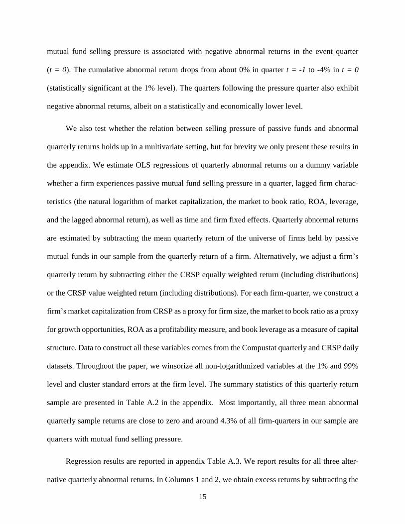
3.6 Cross-sectional tests: Which peers matter?

Up to now, we have treated all firms in a peer group as equally important. In this sub-section,

we are interested in determining whether there are certain peers within a peer group that are more

33

important in shaping earnings management policies at individual firms. For instance, larger, more

profitable, and geographically closer peers might be a more relevant or salient benchmark for in-

dividual firms. Leary and Roberts (2014) show that in the context of capital structure, less success-

ful firms tend to mimic the financing decisions of more successful peers.

In each fiscal year, we split each firm’s peer group along the median of three characteristics:

total assets, ROA, and geographical distance to the sample firm.11 Thus, for each peer group in

each fiscal year, we are able to identify the peer-subgroups of large (small) peers, profitable (un-

profitable) peers, and close (distant) peers. We then calculate the average discretionary accruals

and the fraction of selling pressure for all peer-subgroups. Similar to the IV regressions performed

in Section 3.4, we instrument average peer-subgroup discretionary accruals with the peer-subgroup

fraction of selling pressure. In the second stage, we regress individual firms’ discretionary accruals

on instrumented discretionary accruals from both peer-subgroups, controlling for individual as well

as peer group characteristics and year fixed effects. The results of these regressions are presented

in Table 6. We note that the coefficient on the instrument in the first-stage regressions is significant

at the 1% level for all peer-subgroups across all three columns. In the second stage, however, the

coefficients on the instrumented peer firm discretionary accruals are only significant for the peer-

subgroups consisting of large peers (Column 1), profitable peers (Column 2), and geographically

close peers (Column 3). These findings are consistent with the idea that within a peer group, certain

peer firms matter more than others in shaping earnings management policies at individual firms.

As expected, firms are more likely to observe and replicate actions taken by more visible (i.e.,

larger), more successful (i.e., larger and more profitable), and geographically closer peers.

11 We calculate the median separately for each peer group in each fiscal year to allow for differences in levels across

peer groups and time.

34

4. Conclusion

In this paper, we analyze whether there are peer effects in corporate earnings management.

We overcome the identification problem common to nearly all peer effect papers by using fund

flow-induced selling pressure by passive mutual funds as an exogenous negative shock to stock

prices (e.g., Coval and Stafford, 2007; Khan, Kogan, and Serafeim, 2012). We empirically confirm

that such a shock significantly affects firms’ stock returns. We then show that managers respond

to such exogenous price shocks by adjusting earnings management policies. Specifically, we find

that managers reduce earnings management following significant negative abnormal returns due to

increased monitoring. While fund flow-induced selling pressure triggers a reduction in discretion-

ary accruals at the firm experiencing fund flow-induced selling pressure, it is unlikely to directly

affect discretionary accruals at other firms in the peer group.

To identify peer effects, we regress a firm’s discretionary accruals in a fiscal year on the

fraction of peer firms that experience selling pressure, controlling for average peer firm character-

istics, selling pressure at the sample firm, sample firm characteristics, and year and firm fixed ef-

fects. We define peer groups based on the text-based network industry classifications (TNIC) of

Hoberg and Phillips (2016). The results of such regressions suggest that a larger fraction of peer

firms experiencing selling pressure is associated with a significant reduction in discretionary ac-

cruals at our sample firms. Specifically, we find a one standard deviation increase in the fraction

of peer firms experiencing fund flow-induced selling pressure to be associated with a decrease in

discretionary accruals by about 20% of mean discretionary accruals – an economically meaningful

effect. To also determine how firms respond to changes in earnings management of their peers, we

estimate instrumental variables (IV) regressions in which we instrument peer firms’ discretionary

accruals with the fraction of peer firms that experience selling pressure. We find individual firms’

discretionary accruals to be significantly related peer firms’ discretionary accruals. Finally, we

35

show that firms react mostly to changes in earnings management of large, profitable, and geograph-

ically close peers.

36

References

Ahern, K., R. Duchin, and T. Shumway, 2014, Peer effects in risk aversion and trust, Review of

Financial Studies 27, 3213-3240.

Banerjee, A., 1992, A simple model of herd behavior, Quarterly Journal of Economics 107, 797-

817.

Bikhchandani, S., D. Hirshleifer, and I. Welch, 1992, A theory of fads, fashion, custom, and cul-

tural change as informational cascades, Journal of Political Economy 100, 992-1026.

Bizjak, J., M. Lemmon, and L. Naveen, 2008, Does the use of peer groups contribute to higher pay

and less efficient compensation?, Journal of Financial Economics 90, 152-168.

Bizjak, J., M. Lemmon, and T. Nguyen, 2011, Are all CEOs above average? An empirical analysis

of compensation peer groups and pay design, Journal of Financial Economics 100, 538-555.

Cao, J., H. Liang, and X. Zhan, 2016, Peer effects of corporate social responsibility, Working Pa-

per, Chinese University of Hong Kong.

Chang, T., D. Solomon, and M. Westerfield, 2016, Looking for someone to blame: Delegation,

cognitive dissonance, and the disposition effect, Journal of Finance 71, 267-302.

Cohen, L., and A. Frazzini, 2008, Economic links and predictable returns, Journal of Finance 63,

1977-2011.

Coval, J., and E. Stafford, 2007, Asset fire sales (and purchases) in equity markets, Journal of

Financial Economics 86, 479-512.

Das, S., and H. Zhang, 2003, Rounding-up in reported EPS, behavioral thresholds, and earnings

management, Journal of Accounting and Economics 35, 31-50.

DeAngelo, L., 1981, Auditor independence, ‘low balling’, and disclosure regulation, Journal of

Accounting and Economics 3, 113-127.

Dechow, P., and I. Dichev, 2002, The quality of accruals and earnings: The role of accrual estima-

tion errors, Accounting Review 77, 35-59.

Dechow, P., R. Sloan, and A. Sweeney, 1995, Detecting earnings management, Accounting Review

70, 193-225.

Dechow, P., W. Ge, and C. Schrand, 2010, Understanding earnings quality: A review of the prox-

ies, their determinants and their consequences, Journal of Accounting and Economics 50, 344-401.

DeFond, M., and C. Park, 1997, Smoothing income in anticipation of future earnings, Journal of

Accounting and Economics 23, 115-139.

Dichev, I., J. Graham, C. Harvey, and S. Rajgopal, 2013, Earnings quality: Evidence from the field,

Journal of Accounting and Economics 56, 1-33.

Dyck, A., A. Morse, and L. Zingales, 2010, Who blows the whistle on corporate fraud?, Journal

of Finance 65, 2213-2253.

37

Edmans, A., I. Goldstein, and W. Jiang, 2012, The real effects of financial markets: The impact of

prices on takeovers, Journal of Finance 67, 933-971.

Fang, V., A. Huang, and J. Karpoff, 2016, Short selling and earnings management: A controlled

experiment, Journal of Finance 71, 1251-1294.

Fishman, M., and K. Hagerty, 1992, Insider trading and the efficiency of stock prices, Rand Journal

of Economics 23, 106-122.

Foucault, T., and L. Fresard, 2014, Learning from peers' stock prices and corporate investment,

Journal of Financial Economics 111, 554-577.

Fracassi, C., 2016, Corporate finance policies and social networks, Management Science, forth-

coming.

Gleason, C., N. Jenkins, and W. Johnson, 2008, The contagion effects of accounting restatements,

Accounting Review 83, 83-100.

Grullon, G., S. Michenaud, and J. Weston, 2015, The real effects of short-selling constraints, Re-

view of Financial Studies 28, 1737-1767.

Hameed, A., R. Morck, J. Shen, and B. Yeung, 2015, Information, analysts, and stock return

comovement, Review of Financial Studies 28, 3153-3187.

Healy, P., and J. Wahlen, 1999, A review of the earnings management literature and its implications

for standard setting, Accounting Horizons 13, 365-383.

Henning, L., D. Oesch, and M. Schmid, 2016, Stock underpricing and firm news disclosure, Work-

ing Paper, University of St. Gallen.

Hoberg, G., G. Phillips, and N. Prabhala, 2014, Product market threats, payouts, and financial flex-

ibility, Journal of Finance 69, 293-324.

Hoberg, G., and G. Phillips, 2016, Text-based network industries and endogenous product differ-

entiation, Journal of Political Economy 124, 1423-1465.

Hope, O., W. Thomas, and D. Vyas, 2013, Financial reporting quality of U.S. private and public

firms, Accounting Review 88, 1715-1742.

Hsu, H.-C, A. Reed, and J. Rocholl, 2010, The new game in town: Competitive effects of IPOs,

Journal of Finance 65, 495-528.

Irani, R., and D. Oesch, 2016, Analyst coverage and real earnings management: Quasi-experi-

mental evidence, Journal of Financial and Quantitative Analysis 51, 589-627.

Jenter, D., and F. Kanaan, 2015, CEO turnover and relative performance evaluation, Journal of

Finance 70, 2155-2183.

Jones, J., 1991, Earnings management during import relief investigations, Journal of Accounting

Research 29, 193-228.

38

Kaustia, M., and V. Rantala, 2015, Social learning and corporate peer effects, Journal of Financial

Economics 117, 653-669.

Khan, M., L. Kogan, and G. Serafeim, 2012, Mutual fund trading pressure: Firm-level stock price

impact and timing of SEOs, Journal of Finance 67, 1371-1395.

Leary, M., and M. Roberts, 2014, Do peer firms affect corporate financial policy?, Journal of Fi-

nance 69, 139-178.

Lee, G., and R. Masulis, 2009, Seasoned equity offerings: Quality of accounting information and

expected flotation costs, Journal of Financial Economics 92, 443-469.

Leuz, C., D. Nanda, and P. Wysocki, 2003, Earnings management and investor protection: An

international comparison, Journal of Financial Economics 69, 505-527.

Lou, D., 2012, A flow-based explanation for return predictability, Review of Financial Studies 25,

3457-3489.

Manski, C., 1993, Identification of endogenous social effects: The reflection problem, Review of

Economic Studies 60, 531-542.

Massa, M., B. Zhang, and H. Zhang, 2015, The invisible hand of short selling: Does short selling

discipline earnings management?, Review of Financial Studies 28, 1701-1736.

McNichols, M., 2004, Discussion of the quality of accruals and earnings: The role of accrual esti-

mation errors, Accounting Review 77, 61-69.

Morsfield, S., and C. Tan, 2006, Do venture capitalists influence the decision to manage earnings

in initial public offerings?, Accounting Review 81, 1119-1150.

Muslu, V., M. Rebello, and Y. Xu, 2014, Sell-side analyst research and stock comovement, Journal

of Accounting Research 52, 911-954.

Nissim, D., and S. Penman, 2001, Ratio analysis and equity valuation: From research to practice,

Review of Accounting Studies 6, 109-154.

Servaes, H., and A. Tamayo, 2014, How do industry peers respond to control threats?, Management

Science 60, 380-399.

Shue, K., 2013, Executive networks and firm policies: Evidence from the random assignment of

MBA peers, Review of Financial Studies 26, 1401-1442.

Stubben, S., 2010, Discretionary revenues as a measure of earnings management, Accounting Re-

view 85, 695-717.

Watts, R., and J. Zimmerman, 1986, Positive accounting theory, Englewood Cliffs, NJ, Prentice-

Hall.

Zwiebel, J., 1995, Corporate conservatism and relative compensation, Journal of Political Econ-

omy 103, 1-25.

39

Figure 1: Cumulative average abnormal return around pressure quarters

This figure displays the quarterly cumulative average abnormal return in percent around selling pressure quarters. The sample includes firm-quarters

of all non-financial and non-utility firms from Compustat Quarterly for the period 2000 to 2014 with CRSP share code 10 or 11, for which passive

mutual fund flow-induced selling pressure can be calculated and for which at least three peers can be identified. Peers are identified using the text-

based industry classifications of Hoberg and Phillips (2016). For each firm-quarter observation, the abnormal return is calculated as a firm’s quarterly

return minus the mean quarterly return of the universe of firms held by passive mutual funds in the sample in that quarter. Cumulative average abnormal

returns are the running sum of the average abnormal returns starting in t-3. Selling pressure occurs in quarter t = 0. The time increments are in quarters.

To ensure that t = 0 is the only quarter with selling pressure, the figure only displays the average abnormal return of firms that experience exactly one

quarter of selling pressure. A calendar quarter is defined as a selling pressure quarter if Pressure_CS is in the lowest decile and UPressure is in one of

the middle four deciles (4, 5, 6 or 7). Pressure_CS is calculated as in Coval and Stafford (2007) and UPressure as in Khan, Kogan, and Serafeim (2012)

using data on holdings of passive funds from the CRSP and Thomson mutual fund databases.

40

Table 1: Summary statistics

This table reports selected summary statistics. The sample includes firm-years of all non-financial and non-utility firms from Compustat for the period

2000 to 2014 with CRSP share code 10 or 11, for which passive mutual fund flow-induced selling pressure can be calculated and for which at least

three peers can be identified. Peers are identified using the text-based industry classifications of Hoberg and Phillips (2016). Firm-specific character-

istics reported in Panel A are individual firm characteristics, while peer group averages reported in Panel B are calculated as the mean across all firms

in a peer group for a given characteristic. Discretionary accruals are in % of total assets from the modified Jones model (Dechow, Sloan, and Sweeney,

1995), the Jones (1991) model, the modified Dechow-Dichev (FDD) model augmented with firm fixed effects (Lee and Masulis, 2009). Discretionary

revenues in % of total assets are from the Stubben (2010) revenue model. Fraction with selling pressure is the average of all selling pressure dummies

for a peer group in a fiscal year. The selling pressure dummy is equal to one if a firm experienced selling pressure in any of the four calendar quarters

preceding the fiscal year end, and zero otherwise. A calendar quarter is defined as a selling pressure quarter if Pressure_CS (Pressure_KKS) is in the

lowest decile and UPressure is in one of the middle four deciles (4, 5, 6, or 7). Pressure_CS is calculated as PRESSURE_1 in Coval and Stafford

(2007), and Pressure_KKS and UPressure as in Khan, Kogan, and Serafeim (2012) using data on holdings of passive funds from the CRSP and

Thomson mutual fund databases. Discretionary accruals, discretionary revenues, market capitalization, market to book, ROA, and leverage are as of

the fiscal year end. All non-logarithmized variables are winsorized at the 1% and 99% level. Detailed variable definitions can be found in Table A.1 in

the appendix.

Mean p25 p50 p75 Std. Dev. N

Panel A: Firm-specific characteristics

Modified Jones model (in % of total assets) 1.109 -5.291 0.865 7.848 16.382 35,086

Jones model 1.180 -5.318 0.887 7.991 16.633 35,086

Modified Dechow-Dichev (FDD) model 4.712 1.486 3.233 6.124 4.926 32,231

Revenue model 3.095 0.755 1.762 3.775 3.909 35,076

Selling pressure (CS) (dummy) 0.139 0.000 0.000 0.000 0.346 35,086

Selling pressure (KKS) (dummy) 0.142 0.000 0.000 0.000 0.349 35,086

Market cap ($millions) 2,972.006 128.497 448.278 1,610.498 8,777.966 35,086

Market to book 2.877 1.167 2.020 3.502 4.102 35,086

ROA 0.052 0.028 0.106 0.164 0.224 35,086

Leverage 0.282 0.005 0.208 0.443 0.309 35,086

Panel B: Peer group averages

Number of peers 58.642 12.000 31.000 78.000 67.218 35,086

Modified Jones model (in % of total assets) 0.311 -2.971 0.088 3.325 6.371 35,086

Jones model 0.436 -2.911 0.139 3.450 6.381 35,086

Modified Dechow-Dichev (FDD) model 4.686 3.545 4.472 5.613 1.728 35,015

Revenue model 3.016 2.123 2.825 3.577 1.417 35,086

Fraction with selling pressure (CS) 0.145 0.045 0.125 0.208 0.128 35,086

Fraction with selling pressure (KKS) 0.151 0.053 0.130 0.215 0.128 35,086

Market cap ($millions) 3,391.101 1,421.237 2,559.762 4,291.613 3,138.647 35,086

Market to book 2.977 1.951 2.723 3.831 1.611 35,086

ROA 0.042 0.010 0.092 0.139 0.144 35,086

Leverage 0.275 0.160 0.246 0.368 0.148 35,086

Geographical distance (km) 1913.988 1464.628 1842.991 2240.002 742.822 35,086

41

Table 2: Selling pressure and earnings management

This table reports results from fixed effects regressions of discretionary accruals on passive mutual fund flow-induced selling pressure. The sample includes firm-years of all non-financial and non-

utility firms from Compustat for the period 2000 to 2014 with CRSP share code 10 or 11, for which passive mutual fund flow-induced selling pressure can be calculated and for which at least three

peers can be identified. Peers are identified using the text-based industry classifications of Hoberg and Phillips (2016). The dependent variable in all specifications is the signed value of discretionary

accruals in % of total assets from the modified Jones model (Dechow, Sloan, and Sweeney, 1995). In all specifications, the selling pressure dummy is equal to one if a firm experienced selling pressure

in any of the four calendar quarters preceding the fiscal year end, and zero otherwise. A calendar quarter is defined as a selling pressure quarter if Pressure_CS (Pressure_KKS) is in the lowest decile

and UPressure is in one of the middle four deciles (4, 5, 6, or 7). Pressure_CS is calculated as PRESSURE_1 in Coval and Stafford (2007), and Pressure_KKS and UPressure as in Khan, Kogan, and

Serafeim (2012) using data on holdings of passive funds from the CRSP and Thomson mutual fund databases. In Columns 3 and 4, Pressure_CS and Pressure_KKS are calculated excluding the max

function of equations (2) and (3), respectively. In Columns 5 and 6, firms that experience more than two quarters of selling pressure during the sample period are excluded. Discretionary accruals,

market capitalization, market to book, ROA, and leverage are as of the fiscal year end. All non-logarithmized variables are winsorized at the 1% and 99% level. Detailed variable definitions can be

found in Table A.1 in the appendix. All regressions include firm and year fixed effects. Standard errors are clustered at the firm level. t-values are shown below the coefficients in parentheses. *, **,

and ***, indicate statistical significance of a two-sided test at the 10%, 5%, and 1% level, respectively.

Dep. Var.: Discretionary accruals from the modified Jones model

Max 2 shocks of selling pressure

(1) (2) (3) (4) (5) (6)

Selling pressure calculated with: Pressure_CS Pressure_KKS Pressure_CS (no max) Pressure_KKS (no max) Pressure_CS Pressure_KKS

Selling pressure (dummy) -0.601*** -0.394* -0.492** -0.394* -0.960*** -0.654**

(-2.803) (-1.857) (-2.268) (-1.843) (-3.026) (-2.047)

Log(market cap) 0.461** 0.459** 0.459** 0.460** 0.578** 0.615**

(2.211) (2.203) (2.201) (2.205) (2.438) (2.570)

Market to book 0.069* 0.069* 0.069* 0.069* 0.068 0.075

(1.776) (1.773) (1.776) (1.772) (1.498) (1.608)

ROA 22.864*** 22.874*** 22.868*** 22.873*** 22.539*** 22.379***

(15.510) (15.512) (15.510) (15.511) (13.946) (13.568)

Leverage -2.720*** -2.712*** -2.721*** -2.711*** -2.805*** -3.167***

(-3.642) (-3.631) (-3.642) (-3.630) (-3.350) (-3.623)

Firm fixed effects Yes Yes Yes Yes Yes Yes

Year fixed effects Yes Yes Yes Yes Yes Yes

Observations 35,086 35,086 35,086 35,086 27,171 26,510

R-squared 0.051 0.051 0.051 0.051 0.053 0.053

Number of firms 5,641 5,641 5,641 5,641 4,996 4,941

42

Table 3: Peer effects in corporate earnings management

This table reports results on peer effects in earnings management from fixed effects regressions of firms’ discretionary accruals in a given year on the

fraction of peer firms that experience selling pressure, controlling for average peer group averages, selling pressure at individual firms, and individual

firm characteristics. The sample includes firm-years of all non-financial and non-utility firms from Compustat for the period 2000 to 2014 with CRSP

share code 10 or 11, for which passive mutual fund flow-induced selling pressure can be calculated and for which at least three peers can be identified.

Peers are identified using the text-based industry classifications of Hoberg and Phillips (2016). The dependent variable in all specifications is the signed

value of discretionary accruals in % of total assets from the modified Jones model (Dechow, Sloan, and Sweeney, 1995). Firm-specific characteristics

are individual firm characteristics, while peer group averages are calculated as the mean across all firms in a peer group for a given characteristic.

Fraction with selling pressure is the average of all selling pressure dummies for a peer group in a fiscal year. The selling pressure dummy is equal to

one if a firm experienced selling pressure in any of the four calendar quarters preceding the fiscal year end, and zero otherwise. A calendar quarter is

defined as a selling pressure quarter if Pressure_CS (Pressure_KKS) is in the lowest decile and UPressure is in one of the middle four deciles (4, 5, 6,

or 7). Pressure_CS is calculated as PRESSURE_1 in Coval and Stafford (2007), and Pressure_KKS and UPressure as in Khan, Kogan, and Serafeim

(2012) using data on holdings of passive funds from the CRSP and Thomson mutual fund databases. In Columns 3 and 4, only firms that do not

experience selling pressure in years t and t-1 are retained in the sample. Therefore, the selling pressure dummy is omitted. Discretionary accruals,

market capitalization, market to book, ROA, and leverage are as of the fiscal year end. All non-logarithmized variables are winsorized at the 1% and

99% level. Detailed variable definitions can be found in Table A.1 in the appendix. All regressions include firm and year fixed effects. Standard errors

are clustered at the firm level. t-values are shown below the coefficients in parentheses. *, **, and ***, indicate statistical significance of a two-sided

test at the 10%, 5%, and 1% level, respectively.

Dep. Var.: Discretionary accruals from the modified Jones model

Only firms without shock in t and t-1

(1) (2) (3) (4)

Selling pressure calculated with: Pressure_CS Pressure_KKS Pressure_CS Pressure_KKS

Peer group averages

Fraction with selling pressure -1.779** -1.798** -2.033** -1.590

(-2.460) (-2.468) (-2.064) (-1.602)

Log(market cap) 0.306 0.308 -0.039 0.059

(1.513) (1.526) (-0.139) (0.218)

Market to book 0.151* 0.152** 0.163 0.185

(1.957) (1.970) (1.433) (1.643)

ROA 3.510* 3.567* 4.073 2.755

(1.653) (1.681) (1.461) (1.007)

Leverage 1.592 1.612 1.213 0.608

(1.288) (1.305) (0.722) (0.362)

Firm-specific characteristics

Selling pressure (dummy) -0.518** -0.315 omitted omitted

(-2.396) (-1.472)

Log(market cap) 0.420** 0.419** 0.513** 0.584**

(1.975) (1.971) (1.968) (2.229)

Market to book 0.065* 0.065* -0.021 -0.014

(1.680) (1.681) (-0.384) (-0.247)

ROA 22.460*** 22.465*** 19.910*** 19.116***

(15.071) (15.069) (10.212) (9.653)

Leverage -2.781*** -2.772*** -5.512*** -5.831***

(-3.710) (-3.699) (-5.940) (-6.125)

Firm fixed effects Yes Yes Yes Yes

Year fixed effects Yes Yes Yes Yes

Observations 35,086 35,086 19,423 19,258

R-squared 0.052 0.052 0.046 0.044

Number of firms 5,641 5,641 4,324 4,330

43

Table 4: Disentangling actions and characteristics

This table reports the change in discretionary accruals, from fiscal year t-1 to t, for 25 different buckets of firms. Buckets are formed along two

dimensions: (1) quintiles of the fraction of peer firms experiencing a shock, given that one peer firm is shocked (displayed vertically), and (2) quintiles

of the average change in discretionary accruals of peer firms (displayed horizontally). The entries are the average change in discretionary accruals for

firms placed in the respective bucket. Signed discretionary accruals are in % of total assets from the modified Jones model (Dechow, Sloan, and

Sweeney, 1995). The sample includes firm-years of all non-financial and non-utility firms from Compustat for the period 2000 to 2014 with CRSP

share code 10 or 11, for which passive mutual fund flow-induced selling pressure can be calculated and for which at least three peers can be identified.

Peers are identified using the text-based industry classifications of Hoberg and Phillips (2016). Results of tests for differences in means between

columns 5 and 1 and rows 5 and 1 are displayed. t-values are shown in parentheses. *, **, and ***, indicate statistical significance of a two-sided test

at the 10%, 5%, and 1% level, respectively.

Peer Firm Average Discretionary Accruals Change - Quintiles

Fraction of Peer Firms

Shocked - Quintiles 1 2 3 4 5 5 - 1

1 -7.055 *** -2.931 *** -0.023 2.292 *** 6.504 *** 13.559 ***

(-9.122) (-4.515) (-0.038) (3.367) (8.246)

2 -6.696 *** -2.160 *** 0.452 2.271 *** 6.412 *** 13.108 ***

(-9.669) (-4.24) (0.896) (4.166) (9.313)

3 -6.133 *** -2.177 *** 0.794 1.831 *** 4.893 *** 11.026 ***

(-7.968) (-3.711) (1.385) (3.144) (6.945)

4 -6.456 *** -1.111 ** 0.882 * 1.076 * 4.273 *** 10.729 ***

(-8.847) (-2.019) (1.645) (1.745) (6.544)

5 -7.180 *** -1.971 *** 0.210 0.845 4.526 *** 11.706 ***

(-10.326) (-3.253) (0.364) (1.279) (6.178)

5 - 1 -0.125 0.960 0.233 -1.446 -1.978 *

44

Table 5: Instrumental variables regressions of peer effects in corporate earnings management

This table reports results from instrumental variable regressions of discretionary accruals on peer firms’ instrumented discretionary accruals. The

sample includes firm-years of all non-financial and non-utility firms from Compustat for the period 2000 to 2014 with CRSP share code 10 or 11, for

which passive mutual fund flow-induced selling pressure can be calculated and for which at least three peers can be identified. Peers are identified

using the text-based industry classifications of Hoberg and Phillips (2016). The dependent variable in all specifications is the signed value of discre-

tionary accruals in % of total assets from the modified Jones model (Dechow, Sloan, and Sweeney, 1995). Firm-specific characteristics are individual

firm characteristics, while peer group averages are calculated as the mean across all firms in a peer group for a given characteristic. Fraction with

selling pressure is the average of all selling pressure dummies for a peer group in a fiscal year. Fraction with selling pressure is the instrument for the

endogenous variable, which is the peer group average value of discretionary accruals from the modified Jones model. The coefficient on the instrument

from the first-stage is reported at the bottom of the table. The selling pressure dummy is equal to one if a firm experienced selling pressure in any of

the four calendar quarters preceding the fiscal year end, and zero otherwise. A calendar quarter is defined as a selling pressure quarter if Pressure_CS

(Pressure_KKS) is in the lowest decile and UPressure is in one of the middle four deciles (4, 5, 6, or 7). Pressure_CS is calculated as PRESSURE_1

in Coval and Stafford (2007), and Pressure_KKS and UPressure as in Khan, Kogan, and Serafeim (2012) using data on holdings of passive funds from

the CRSP and Thomson mutual fund databases. In Columns 3 and 4, only firms that do not experience selling pressure in years t and t-1 are retained

in the sample. Therefore, the selling pressure dummy is omitted. Discretionary accruals, market capitalization, market to book, ROA, and leverage are

as of the fiscal year end. All non-logarithmized variables are winsorized at the 1% and 99% level. Detailed variable definitions can be found in Table

A.1 in the appendix. All regressions include year fixed effects. Standard errors are clustered at the firm level. t-values are shown below the coefficients

in parentheses. *, **, and ***, indicate statistical significance of a two-sided test at the 10%, 5%, and 1% level, respectively.

Dep. Var.: Discretionary accruals from the modified Jones model

Only firms without shock in t and t-1

(1) (2) (3) (4)

Selling Pressure calculated with: Pressure_CS Pressure_KKS Pressure_CS Pressure_KKS

Peer group averages

Discretionary accruals 0.834*** 0.861*** 0.867*** 0.910***

(3.005) (3.798) (2.916) (3.151)

Log(market cap) 0.606*** 0.597*** 0.336 0.306

(3.248) (3.293) (1.253) (1.149)

Market to book -0.022 -0.030 -0.132 -0.103

(-0.214) (-0.325) (-1.125) (-0.875)

ROA -18.323*** -18.679*** -16.976*** -17.253***

(-4.900) (-5.961) (-6.146) (-6.430)

Leverage 2.313 2.149 1.618 1.288

(1.363) (1.476) (0.803) (0.678)

Firm-specific characteristics

Selling pressure (dummy) -0.254 -0.509** omitted omitted

(-1.139) (-2.289)

Log(market cap) -0.387*** -0.371*** -0.265*** -0.245***

(-5.408) (-5.235) (-3.079) (-2.871)

Market to book 0.043 0.042 -0.027 -0.022

(1.323) (1.304) (-0.589) (-0.494)

ROA 17.754*** 17.715*** 14.462*** 14.484***

(18.997) (19.342) (13.147) (13.175)

Leverage -2.581*** -2.583*** -3.086*** -3.298***

(-6.048) (-6.084) (-5.662) (-6.019)

First-stage instrument

Peer firm fraction with selling pressure -2.626*** -3.285*** -3.156*** -3.364***

(-7.690) (-9.521) (-6.662) (-6.982)

Firm fixed effects No No No No

Year fixed effects Yes Yes Yes Yes

Observations 35,086 35,086 19,423 19,258

R-squared 0.121 0.120 0.111 0.109

Number of firms 5,641 5,641 4,324 4,330

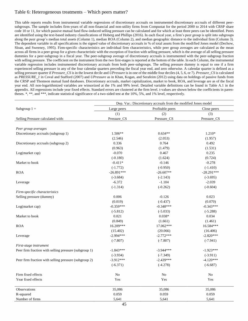
45

Table 6: Heterogeneous treatments – Which peers matter?

This table reports results from instrumental variable regressions of discretionary accruals on instrumented discretionary accruals of different peer-

subgroups. The sample includes firm-years of all non-financial and non-utility firms from Compustat for the period 2000 to 2014 with CRSP share

code 10 or 11, for which passive mutual fund flow-induced selling pressure can be calculated and for which at least three peers can be identified. Peers

are identified using the text-based industry classifications of Hoberg and Phillips (2016). In each fiscal year, a firm’s peer group is split into subgroups

along the peer group’s median total assets (Column 1), median ROA (Column 2), and median geographic distance to the individual firm (Column 3).

The dependent variable in all specifications is the signed value of discretionary accruals in % of total assets from the modified Jones model (Dechow,

Sloan, and Sweeney, 1995). Firm-specific characteristics are individual firm characteristics, while peer group averages are calculated as the mean

across all firms in a peer group for a given characteristic with the exception of fraction with selling pressure, which is the average of all selling pressure

dummies for a peer-subgroup in a fiscal year. The peer-subgroup average of discretionary accruals is instrumented with the peer-subgroup fraction

with selling pressure. The coefficient on the instrument from the two first-stages is reported at the bottom of the table. In each Column, the instrumental

variable regression includes instrumented discretionary accruals from both peer-subgroups. The selling pressure dummy is equal to one if a firm

experienced selling pressure in any of the four calendar quarters preceding the fiscal year end, and zero otherwise. A calendar quarter is defined as a

selling pressure quarter if Pressure_CS is in the lowest decile and UPressure is in one of the middle four deciles (4, 5, 6, or 7). Pressure_CS is calculated

as PRESSURE_1 in Coval and Stafford (2007) and UPressure as in Khan, Kogan, and Serafeim (2012) using data on holdings of passive funds from

the CRSP and Thomson mutual fund databases. Discretionary accruals, market capitalization, market to book, ROA, and leverage are as of the fiscal

year end. All non-logarithmized variables are winsorized at the 1% and 99% level. Detailed variable definitions can be found in Table A.1 in the

appendix. All regressions include year fixed effects. Standard errors are clustered at the firm level. t-values are shown below the coefficients in paren-

theses. *, **, and ***, indicate statistical significance of a two-sided test at the 10%, 5%, and 1% level, respectively.

Dep. Var.: Discretionary accruals from the modified Jones model

Subgroup 1 = Large peers Profitable peers Close peers

(1) (2) (3)

Selling Pressure calculated with: Pressure_CS Pressure_CS Pressure_CS

Peer group averages

Discretionary accruals (subgroup 1) 1.506** 0.634** 1.210*

(2.546) (2.053) (1.957)

Discretionary accruals (subgroup 2) 0.336 0.764 0.492

(0.963) (1.479) (1.531)

Log(market cap) -0.070 0.467 0.235

(-0.180) (1.624) (0.724)

Market to book -0.411* -0.146 -0.278

(-1.772) (-0.950) (-1.410)

ROA -26.891*** -26.607** -28.291***

(-3.684) (-2.143) (-3.695)

Leverage -6.372 -1.104 -2.039

(-1.314) (-0.262) (-0.604)

Firm-specific characteristics

Selling pressure (dummy) 0.006 -0.126 0.023

(0.019) (-0.437) (0.070)

Log(market cap) -0.359*** -0.348*** -0.343***

(-5.812) (-5.033) (-5.288)

Market to book 0.021 0.038* 0.034

(0.849) (1.661) (1.461)

ROA 16.209*** 17.062*** 16.584***

(15.402) (20.066) (16.406)

Leverage -2.994*** -2.772*** -2.820***

(-7.807) (-7.807) (-7.941)

First-stage instrument

Peer firm fraction with selling pressure (subgroup 1) -1.843*** -3.944*** -1.923***

(-3.934) (-7.349) (-3.911)

Peer firm fraction with selling pressure (subgroup 2) -3.912*** -2.439*** -4.120***

(-6.371) (-4.278) (-6.687)

Firm fixed effects No No No

Year fixed effects Yes Yes Yes

Observations 35,086 35,086 35,086

R-squared 0.059 0.059 0.059

Number of firms 5,641 5,641 5,641

46

Appendix

Figure A.1.: Distribution of selling pressure quarters during the sample period

This figure displays the distribution of selling pressure over the sample period. The sample includes firm-quarters of all non-financial and non-utility

firms from Compustat for the period 2000 to 2014 with CRSP share code 10 or 11, for which passive mutual fund flow-induced selling pressure can

be calculated and for which at least three peers can be identified. Peers are identified using the text-based industry classifications of Hoberg and Phillips

(2016). Time increments are in calendar quarters. In each calendar quarter, the density of firms that experience selling pressure is displayed. A calendar

quarter is defined as a selling pressure quarter if Pressure_CS is in the lowest decile and UPressure is in one of the middle four deciles (4, 5, 6 or 7).

Pressure_CS is calculated as PRESSURE_1 in Coval and Stafford (2007) and UPressure as in Khan, Kogan, and Serafeim (2012) using data on holdings

of passive funds from the CRSP and Thomson mutual fund databases. The red vertical lines indicate the fourth calendar quarter of each year.

47

Table A.1: Variable definitions

Variable Definition

Selling pressure measures

Selling pressure (dummy) using Pressure_CS

in quarterly sample

A dummy variable that equals one if there is selling pressure in the calendar quarter, and zero otherwise.

A calendar quarter is defined as a selling pressure quarter if Pressure_CS is in the lowest decile and UPres-

sure is in one of the middle four deciles (4, 5, 6 or 7). Deciles are calculated for every quarter separately.

Pressure_CS is constructed as PRESSURE_1 in Coval and Stafford (2007) and UPressure as in Khan,

Kogan, and Serafeim (2012). Only the holdings of passive funds are used to construct these measures.

Selling pressure (dummy) using Pressure_KKS

in quarterly sample

A dummy variable that equals one if there is selling pressure in the calendar quarter, and zero otherwise.

A calendar quarter is defined as a selling pressure quarter if Pressure_KKS is in the lowest decile and

UPressure is in one of the middle four deciles (4, 5, 6 or 7). Deciles are calculated for every quarter sepa-

rately. Pressure_KKS and UPressure are constructed like the pressure measures used in Khan, Kogan, and

Serafeim (2012). Only the holdings of passive funds are used to construct these measures.

Selling pressure (dummy) using Pressure_CS

in yearly sample

A dummy variable that equals one if there was selling pressure in any of the four calendar quarters preced-

ing the fiscal year end, and zero otherwise. A calendar quarter is defined as a selling pressure quarter if

Pressure_CS is in the lowest decile and UPressure is in one of the middle four deciles (4, 5, 6 or 7). Deciles

are calculated for every quarter separately. Pressure_CS is constructed as PRESSURE_1 in Coval and

Stafford (2007) and UPressure as in Khan, Kogan, and Serafeim (2012). Only the holdings of passive

funds are used to construct these measures.

Selling pressure (dummy) using Pressure_KKS

in yearly sample

A dummy variable that equals one if there was selling pressure in any of the four calendar quarters preced-

ing the fiscal year end, and zero otherwise. A calendar quarter is defined as a selling pressure quarter if

Pressure_KKS is in the lowest decile and UPressure is in one of the middle four deciles (4, 5, 6 or 7).

Deciles are calculated for every quarter separately. Pressure_KKS and UPressure are constructed like the

pressure measures used in Khan, Kogan, and Serafeim (2012). Only the holdings of passive funds are used

to construct these measures.

Fraction with selling pressure

using Pressure_CS

The fraction of firms in a peer group that experience selling pressure in a fiscal year. For each peer group

in each fiscal year, the average of all yearly selling pressure dummies (based on Pressure_CS) is calculated.

This variable is bounded by zero and one.

Fraction with selling pressure

using Pressure_KKS

The fraction of firms in a peer group that experience selling pressure in a fiscal year. For each peer group

in each fiscal year, the average of all yearly selling pressure dummies (based on Pressure_KKS) is calcu-

lated. This variable is bounded by zero and one.

48

Earnings management measures

Modified Jones model Signed value of discretionary accruals from the modified Jones model (Dechow, Sloan, and

Sweeney,1995), constructed as in Irani and Oesch (2016). Discretionary accruals are the difference be-

tween a firm's actual accruals and its predicted accruals from the modified Jones model. The model is run

for each fiscal year and Fama-French 48 industry separately. A minimum of 20 observations per fiscal

year-industry regression is required for years t through t-4. This variable is in % of total assets.

Jones model Signed value of discretionary accruals from the Jones (1991) model, constructed as in Irani and Oesch

(2016). Discretionary accruals are the difference between a firm's actual accruals and its predicted accruals

from the Jones (1991) model. The model is run for each fiscal year and Fama-French 48 industry sepa-

rately. A minimum of 20 observations per fiscal year-industry regression is required for years t through t-

4. This variable is in % of total assets.

Modified Dechow-Dichev model Absolute value of discretionary accruals from the modified Dechow-Dichev model (McNichols, 2004)

augmented with firm fixed effects, constructed as in Lee and Masulis (2009). Discretionary accruals are

the difference between a firm's actual accruals and its predicted accruals from the modified Dechow-

Dichev model augmented with firm fixed effects in the estimation of accruals. The fixed effects model is

run only once over the entire panel of firms. This variable is in % of total assets.

Revenue model Absolute value of discretionary revenues from the Stubben (2010) revenue model, constructed as in Hope,

Thomas, and Vyas (2013). Discretionary revenues are the difference between a firm’s actual change in

accounts receivable and its predicted change in accounts receivable from the model. The model is run for

each fiscal year and Fama-French 48 industry separately. A minimum of 20 observations per fiscal year-

industry regression is required for years t through t-4. This variable is in % of total assets.

Control variables

Log(market cap) in quarterly sample Natural logarithm of the market value of equity. The market value of equity is calculated with data from

CRSP, by multiplying the closing price with the number of shares outstanding on the last trading day of

the fiscal quarter. Log(market cap) quarterly = ln(1000*shrout*abs(prc)).

Market to book in quarterly sample Market value of equity divided by the book value of equity at the end of the fiscal quarter. The market

value of equity is calculated with data from CRSP, by multiplying the closing price with the number of

shares outstanding on the last trading day of the fiscal quarter. Market value of equity in $ =

abs(prc)*shrout*1,000. Book value of equity is from Compustat, as of the end of the fiscal quarter. Book

value of equity in $ = ceqq*1,000,000.

ROA in quarterly sample Operating income before depreciation of the fiscal quarter scaled by the book value of assets at the end of

the fiscal quarter. ROA quarterly = oibdpq/atq.

49

Leverage in quarterly sample Leverage as of the end of the fiscal quarter, calculated as in Fang, Huang, and Karpoff (2016). Long-term

debt plus debt in current liabilities is divided by the sum of long-term debt, debt in current liabilities, and

total shareholder's equity.

Leverage quarterly = (dlttq + dlcq)/(dlttq + dlcq + seqq).

Log(market cap) in yearly sample Natural logarithm of the market value of equity as of the fiscal year end. Market value of equity is calcu-

lated with data from CRSP, by multiplying the closing price with the number of shares outstanding on the

last trading day of the fiscal year. Log(market cap) = ln(1000*shrout*abs(prc))

Market to book in yearly sample Market value of equity divided by the book value of equity as of the fiscal year end. Market value of equity

is calculated with data from CRSP, by multiplying the closing price with the number of shares outstanding

on the last trading day of the fiscal year. Market value of equity in $ = abs(prc)*shrout*1,000. Book value

of equity is from Compustat, as of the fiscal year end. Book value of equity in $ = ceq*1,000,000

ROA in yearly sample Operating income before depreciation scaled by the book value of assets at the fiscal year end. ROA =

oibdp/at

Leverage in yearly sample Leverage as of the fiscal year end, calculated as in Fang, Huang, and Karpoff (2016). Long-term debt plus

debt in current liabilities is divided by the sum of long-term debt, debt in current liabilities, and total share-

holder's equity.

Leverage = (dltt + dlc)/(dltt + dlc + seq)

Abnormal returns

Return - Sample mean return Abnormal quarterly return in % measured as the firm's quarterly return minus the mean quarterly return of

all firms in the sample. Return data is from CRSP.

Return - CRSP equally weighted return Abnormal quarterly return in % measured as the firm's quarterly return minus the CRSP equally weighted

return including distributions. Return data is from CRSP.

Return - CRSP value weighted return Abnormal quarterly return in % measured as the firm's quarterly return minus the CRSP value weighted

return including distributions. Return data is from CRSP.

50

Table A.2: Summary statistics of quarterly data

This table reports selected summary statistics for the firm-quarter sample. The sample includes firm-quarters of all non-financial and non-utility firms

from Compustat for the period 2000 to 2014 with CRSP share code 10 or 11, for which passive mutual fund flow-induced selling pressure can be

calculated and for which at least three peers can be identified. Peers are identified using the text-based industry classifications of Hoberg and Phillips

(2016). The three abnormal returns are market-adjusted quarterly abnormal returns. A firm’s quarterly return is adjusted by subtracting either (1) the

mean quarterly return of the universe of firms held by passive mutual funds in our sample, (2) the CRSP equally weighted return including distributions,

or (3) the CRSP value weighted return including distributions. The selling pressure dummy is equal to one if a firm experiences selling pressure in a

quarter, and zero otherwise. A calendar quarter is defined as a selling pressure quarter if Pressure_CS (Pressure_KKS) is in the lowest decile and

UPressure is in one of the middle four deciles (4, 5, 6, or 7). Pressure_CS is calculated as PRESSURE_1 in Coval and Stafford (2007), and Pres-

sure_KKS and UPressure as in Khan, Kogan, and Serafeim (2012) using data on holdings of passive funds from the CRSP and Thomson mutual fund

databases. Abnormal returns, market capitalization, market to book, ROA, and leverage are as of the end of the fiscal quarter. Selling pressure dummies

are as of the end of the most recent calendar quarter. All non-logarithmized variables are winsorized at the 1% and 99% level. Detailed variable

definitions can be found in Table A.1 in the appendix.

Mean p25 p50 p75 Std. Dev. N

Abnormal return (in %)

Return - Sample mean return -0.263 -11.201 -1.110 9.044 19.433 146,535

Return - CRSP equally weighted return -0.048 -10.892 -0.778 9.212 19.498 146,535

Return - CRSP value weighted return 0.619 -10.098 -0.222 9.768 19.722 146,535

Selling pressure dummies

Selling pressure (CS) (dummy) 0.043 0.000 0.000 0.000 0.203 146,535

Selling pressure (KKS) (dummy) 0.043 0.000 0.000 0.000 0.204 146,535

Controls

Market cap ($millions) 3,050.494 132.318 461.621 1,660.800 8,964.997 146,535

Market to book 2.983 1.196 2.048 3.555 4.352 146,535

ROA 0.016 0.007 0.028 0.044 0.057 146,535

Leverage 0.283 0.007 0.216 0.446 0.302 146,535

51

Table A.3: Selling pressure and stock returns

This table reports results from fixed effects regressions of firms’ abnormal returns on quarterly selling pressure. The sample includes firm-quarters of all non-financial and non-utility firms from

Compustat for the period 2000 to 2014 with CRSP share code 10 or 11, for which passive mutual fund flow-induced selling pressure can be calculated and for which at least three peers can be identified.

Peers are identified using the text-based industry classifications of Hoberg and Phillips (2016). In all specifications, the dependent variable is the market-adjusted quarterly abnormal return. In Columns

1 and 2, the quarterly abnormal return in % is calculated as a firm’s quarterly return minus the mean quarterly return of the universe of firms held by passive mutual funds in the sample in that quarter.

In Columns 3 and 4, the quarterly abnormal return is calculated as a firm’s quarterly return minus the CRSP equally weighted return including distributions. In Columns 5 and 6, the quarterly abnormal

return is calculated as a firm’s quarterly return minus the CRSP value weighted return including distributions. In all specifications, the selling pressure dummy is equal to one if a firm experiences

selling pressure in that quarter, and zero otherwise. A calendar quarter is defined as a selling pressure quarter if Pressure_CS (Pressure_KKS) is in the lowest decile and UPressure is in one of the

middle four deciles (4, 5, 6, or 7). Pressure_CS is calculated as PRESSURE_1 in Coval and Stafford (2007), and Pressure_KKS and UPressure as in Khan, Kogan, and Serafeim (2012) using data on

holdings of passive funds from the CRSP and Thomson mutual fund databases. The selling pressure dummy is contemporaneous and all control variables are lagged by one quarter. Abnormal returns,

market capitalization, market to book, ROA, and leverage are as of the end of the lagged fiscal quarter. Selling pressure dummies are as of the end of the most recent calendar quarter. All non-

logarithmized variables are winsorized at the 1% and 99% level. Detailed variable definitions can be found in Table A.1 in the appendix. All regressions include firm and year-quarter fixed effects.

Standard errors are clustered at the firm level. t-values are shown below the coefficients in parentheses. *, **, and ***, indicate statistical significance of a two-sided test at the 10%, 5%, and 1% level,

respectively.

Dep. Var.: Abnormal return

Abnormal return by subtracting Sample mean CRSP EW CRSP VW

(1) (2) (3) (4) (5) (6)

Selling pressure calculated with: Pressure_CS Pressure_KKS Pressure_CS Pressure_KKS Pressure_CS Pressure_KKS

Selling pressure (dummy) -0.920*** -1.197*** -0.919*** -1.196*** -0.916*** -1.183***

(-3.637) (-4.734) (-3.638) (-4.732) (-3.629) (-4.683)

Log(market cap) -5.863*** -5.855*** -5.851*** -5.844*** -5.831*** -5.824***

(-64.660) (-64.562) (-64.555) (-64.457) (-64.397) (-64.301)

Market to book 0.028* 0.028* 0.027* 0.028* 0.027* 0.027*

(1.893) (1.901) (1.852) (1.861) (1.834) (1.843)

ROA 51.981*** 52.010*** 52.003*** 52.032*** 52.195*** 52.224***

(30.018) (30.036) (30.041) (30.059) (30.181) (30.199)

Leverage -1.844*** -1.839*** -1.851*** -1.847*** -1.808*** -1.804***

(-5.614) (-5.601) (-5.638) (-5.625) (-5.513) (-5.499)

Lagged abnormal return 0.008*** 0.008*** 0.008*** 0.008*** 0.008*** 0.008***

(2.912) (2.899) (2.945) (2.933) (2.924) (2.912)

Firm fixed effects Yes Yes Yes Yes Yes Yes

Year-quarter fixed effects Yes Yes Yes Yes Yes Yes

Observations 137,252 137,252 137,252 137,252 137,252 137,252

R-squared 0.038 0.038 0.043 0.043 0.067 0.067

Number of firms 5,461 5,461 5,461 5,461 5,461 5,461

52

Table A.4: Frequency distribution of selling pressure quarters per firm

This table reports the number of selling pressure quarters each distinct firm experiences during the sample period. The sample includes firm-quarters

of all non-financial and non-utility firms from Compustat for the period 2000 to 2014 with CRSP share code 10 or 11, for which passive mutual fund

flow-induced selling pressure can be calculated and for which at least three peers can be identified. Peers are identified using the text-based industry

classifications of Hoberg and Phillips (2016). A calendar quarter is defined as a selling pressure quarter if Pressure_CS is in the lowest decile and

UPressure is in one of the middle four deciles (4, 5, 6, or 7). Pressure_CS is calculated as PRESSURE_1 in Coval and Stafford (2007) and UPressure

as in Khan, Kogan, and Serafeim (2012) using data on holdings of passive funds from the CRSP and Thomson mutual fund databases.

Number of quarters with selling pressure per firm N % Cumulative %

0 2,892 51.27 51.27

1 1,101 19.52 70.79

2 665 11.79 82.57

3 409 7.25 89.82

4 221 3.92 93.74

5 138 2.45 96.19

6 84 1.49 97.68

7 50 0.89 98.56

8 30 0.53 99.10

9 21 0.37 99.47

10 17 0.30 99.77

11 7 0.12 99.89

12 3 0.05 99.95

13 2 0.04 99.98

14 1 0.02 100

Total 5,641 100 -

53

Table A.5: Selling pressure and earnings management – robustness to earnings management measure

This table reports results from fixed effects regressions of alternative measures of earnings management on passive mutual fund flow-induced selling pressure. The sample includes firm-years of all

non-financial and non-utility firms from Compustat for the period 2000 to 2014 with CRSP share code 10 or 11, for which passive mutual fund flow-induced selling pressure can be calculated and for

which at least three peers can be identified. Peers are identified using the text-based industry classifications of Hoberg and Phillips (2016). In Columns 1 and 2, the dependent variable is the signed value

of discretionary accruals in % of total assets from the Jones (1991) model, in Columns 3 and 4 it is the absolute value of discretionary accruals from the modified Dechow-Dichev (FDD) model

augmented with firm fixed effects (Lee and Masulis, 2009), and in Columns 5 and 6 it is the absolute value of discretionary revenues from the Stubben (2010) revenue model. In all specifications, the

selling pressure dummy is equal to one if a firm experienced selling pressure in any of the four calendar quarters preceding the fiscal year end, and zero otherwise. A calendar quarter is defined as a

selling pressure quarter if Pressure_CS (Pressure_KKS) is in the lowest decile and UPressure is in one of the middle four deciles (4, 5, 6, or 7). Pressure_CS is calculated as PRESSURE_1 in Coval

and Stafford (2007), and Pressure_KKS and UPressure as in Khan, Kogan, and Serafeim (2012) using data on holdings of passive funds from the CRSP and Thomson mutual fund databases. Discre-

tionary accruals, discretionary revenues, market capitalization, market to book, ROA, and leverage are as of the fiscal year end. All non-logarithmized variables are winsorized at the 1% and 99% level.

Detailed variable definitions can be found in Table A.1 in the appendix. All regressions include firm and year fixed effects. Standard errors are clustered at the firm level. t-values are shown below the

coefficients in parentheses. *, **, and ***, indicate statistical significance of a two-sided test at the 10%, 5%, and 1% level, respectively.

Dep. Var.: Earnings management measure

Discretionary accruals/revenues from: Jones model FDD model Revenue model

(1) (2) (3) (4) (5) (6)

Selling pressure calculated with: Pressure_CS Pressure_KKS Pressure_CS Pressure_KKS Pressure_CS Pressure_KKS

Selling pressure (dummy) -0.583*** -0.375* -0.158** -0.158** -0.142*** -0.150***

(-2.664) (-1.734) (-2.401) (-2.374) (-2.887) (-3.017)

Log(market cap) 0.516** 0.514** -0.243*** -0.242*** 0.097** 0.098**

(2.453) (2.445) (-4.127) (-4.110) (2.275) (2.299)

Market to book 0.073* 0.073* 0.069*** 0.069*** 0.028*** 0.028***

(1.882) (1.879) (5.718) (5.714) (3.822) (3.812)

ROA 22.881*** 22.890*** -2.186*** -2.185*** 1.757*** 1.756***

(15.279) (15.281) (-4.913) (-4.913) (6.098) (6.097)

Leverage -2.721*** -2.714*** 0.595** 0.597** 0.443*** 0.444***

(-3.591) (-3.581) (2.429) (2.436) (2.912) (2.925)

Firm fixed effects Yes Yes Yes Yes Yes Yes

Year fixed effects Yes Yes Yes Yes Yes Yes

Observations 35,086 35,086 32,231 32,231 35,076 35,076

R-squared 0.051 0.051 0.019 0.019 0.029 0.029

Number of firms 5,641 5,641 5,092 5,092 5,641 5,641

54

Table A.6: Peer effects in corporate earnings management – robustness to pressure measure

This table reports results of robustness checks with regard to the selling pressure measure for the instrumental variable regressions of discretionary

accruals on peer firms’ instrumented discretionary accruals. The sample includes firm-years of all non-financial and non-utility firms from Compustat

for the period 2000 to 2014 with CRSP share code 10 or 11, for which passive mutual fund flow-induced selling pressure can be calculated and for

which at least three peers can be identified. Peers are identified using the text-based industry classifications of Hoberg and Phillips (2016). The de-

pendent variable in all specifications is the signed value of discretionary accruals in % of total assets from the modified Jones model (Dechow, Sloan,

and Sweeney, 1995). Firm-specific characteristics are individual firm characteristics, while peer group averages are calculated as the mean across all

firms in a peer group for a given characteristic. Fraction with selling pressure is the average of all selling pressure dummies for a peer group in a fiscal

year. Fraction with selling pressure is the instrument for the endogenous variable, which is the peer group average value of discretionary accruals from

the modified Jones model. The coefficient on the instrument from the first-stage is reported at the bottom of the table. The selling pressure dummy is

equal to one if a firm experienced selling pressure in any of the four calendar quarters preceding the fiscal year end, and zero otherwise. A calendar

quarter is defined as a selling pressure quarter if Pressure_CS (Pressure_KKS) is in the lowest decile and UPressure is in one of the middle four deciles

(4, 5, 6, or 7). Pressure_CS and Pressure_KKS are calculated excluding the max function of equations (2) and (3), respectively, using data on holdings

of passive funds from the CRSP and Thomson mutual fund databases. In Columns 3 and 4, only firms that do not experience selling pressure in years

t and t-1 are retained in the sample. Therefore, the selling pressure dummy is omitted. Discretionary accruals, market capitalization, market to book,

ROA, and leverage are as of the fiscal year end. All non-logarithmized variables are winsorized at the 1% and 99% level. Detailed variable definitions

can be found in Table A.1 in the appendix. All regressions include year fixed effects. Standard errors are clustered at the firm level. t-values are shown

below the coefficients in parentheses. *, **, and ***, indicate statistical significance of a two-sided test at the 10%, 5%, and 1% level, respectively.

Dep. Var.: Discretionary accruals from the modified Jones model

Only firms without shock in t and t-1

(1) (2) (3) (4)

Selling Pressure calculated with: Pressure_CS (no max) Pressure_KKS (no max) Pressure_CS (no max) Pressure_KKS (no max)

Peer group averages

Discretionary accruals 0.719** 0.746*** 0.797** 0.754***

(2.409) (3.434) (2.504) (2.844)

Log(market cap) 0.647*** 0.639*** 0.385 0.357

(3.404) (3.555) (1.389) (1.379)

Market to book 0.011 0.002 -0.124 -0.071

(0.102) (0.023) (-1.022) (-0.639)

ROA -16.865*** -17.238*** -16.473*** -16.108***

(-4.225) (-5.699) (-5.717) (-6.389)

Leverage 2.931 2.761* 2.275 2.329

(1.637) (1.951) (1.082) (1.299)

Firm-specific characteristics

Selling pressure (dummy) -0.239 -0.611*** omitted omitted

(-1.073) (-2.787)

Log(market cap) -0.395*** -0.374*** -0.257*** -0.219**

(-5.450) (-5.246) (-2.996) (-2.537)

Market to book 0.045 0.044 -0.014 -0.019

(1.367) (1.345) (-0.305) (-0.422)

ROA 17.903*** 17.861*** 14.428*** 14.585***

(18.893) (19.579) (13.092) (13.359)

Leverage -2.550*** -2.550*** -3.121*** -3.267***

(-5.944) (-5.995) (-5.680) (-5.920)

First-stage instrument

Peer firm fraction with selling pressure -2.452*** -3.406*** -2.926*** -3.529***

(-7.041) (-9.909) (-6.111) (-7.393)

Firm fixed effects No No No No

Year fixed effects Yes Yes Yes Yes

Observations 35,086 35,086 19,448 19,280

R-squared 0.123 0.123 0.112 0.113

Number of firms 5,641 5,641 4,328 4,338

55

Table A.7: Peer effects in corporate earnings management – robustness to peer group definition

This table reports results of robustness checks with regard to the peer group definition for the instrumental variable regressions of discretionary accruals

on peer firms’ instrumented discretionary accruals. The sample includes firm-years of all non-financial and non-utility firms from Compustat for the

period 2000 to 2014 with CRSP share code 10 or 11, for which passive mutual fund flow-induced selling pressure can be calculated and for which at

least three peers can be identified. Peers are identified using three-digit SIC industries. The dependent variable in all specifications is the signed value

of discretionary accruals in % of total assets from the modified Jones model (Dechow, Sloan, and Sweeney, 1995). Firm-specific characteristics are

individual firm characteristics, while peer group averages are calculated as the mean across all firms in a peer group for a given characteristic. Fraction

with selling pressure is the average of all selling pressure dummies for a peer group in a fiscal year. Fraction with selling pressure is the instrument for

the endogenous variable, which is the peer group average value of discretionary accruals from the modified Jones model. The coefficient on the

instrument from the first-stage is reported at the bottom of the table. The selling pressure dummy is equal to one if a firm experienced selling pressure

in any of the four calendar quarters preceding the fiscal year end, and zero otherwise. A calendar quarter is defined as a selling pressure quarter if

Pressure_CS (Pressure_KKS) is in the lowest decile and UPressure is in one of the middle four deciles (4, 5, 6, or 7). Pressure_CS is calculated as

PRESSURE_1 in Coval and Stafford (2007), and Pressure_KKS and UPressure as in Khan, Kogan, and Serafeim (2012) using data on holdings of

passive funds from the CRSP and Thomson mutual fund databases. In Columns 3 and 4, only firms that do not experience selling pressure in years t

and t-1 are retained in the sample. Therefore, the selling pressure dummy is omitted. Discretionary accruals, market capitalization, market to book,

ROA, and leverage are as of the fiscal year end. All non-logarithmized variables are winsorized at the 1% and 99% level. Detailed variable definitions

can be found in Table A.1 in the appendix. All regressions include year fixed effects. Standard errors are clustered at the firm level. t-values are shown

below the coefficients in parentheses. *, **, and ***, indicate statistical significance of a two-sided test at the 10%, 5%, and 1% level, respectively.

Dep. Var.: Discretionary accruals from the modified Jones model

Only firms without shock in t and t-1

(1) (2) (3) (4)

Selling Pressure calculated with: Pressure_CS Pressure_KKS Pressure_CS Pressure_KKS

Peer group averages

Discretionary accruals 1.040*** 0.999*** 0.929** 0.884***

(2.814) (4.040) (2.132) (2.951)

Log(market cap) 0.491 0.526** 0.410 0.509

(1.419) (2.098) (0.844) (1.444)

Market to book 0.032 0.040 0.084 0.105

(0.325) (0.510) (0.604) (1.005)

ROA -24.434*** -24.154*** -22.675*** -22.355***

(-8.034) (-10.540) (-10.068) (-11.290)

Leverage 2.147 2.250** 2.573 2.679**

(1.635) (2.193) (1.532) (2.114)

Firm-specific characteristics

Selling pressure (dummy) -0.307 -0.512***

(-1.576) (-2.583)

Log(market cap) -0.583*** -0.569*** -0.541*** -0.530***

(-8.714) (-8.832) (-6.304) (-6.452)

Market to book -0.003 -0.003 -0.047 -0.042

(-0.102) (-0.094) (-1.233) (-1.098)

ROA 21.956*** 21.927*** 18.920*** 18.791***

(27.473) (27.776) (19.677) (19.873)

Leverage -2.159*** -2.138*** -2.689*** -2.868***

(-5.242) (-5.387) (-5.009) (-5.755)

First-stage instrument

Peer firm fraction with selling pressure -1.826*** -2.831*** -1.934*** -2.842***

(-4.588) (-6.788) (-3.716) (-5.367)

Firm fixed effects No No No No

Year fixed effects Yes Yes Yes Yes

Observations 39,334 39,334 22,315 22,254

R-squared 0.173 0.177 0.186 0.190

Number of firms 6,011 6,011 4,704 4,719

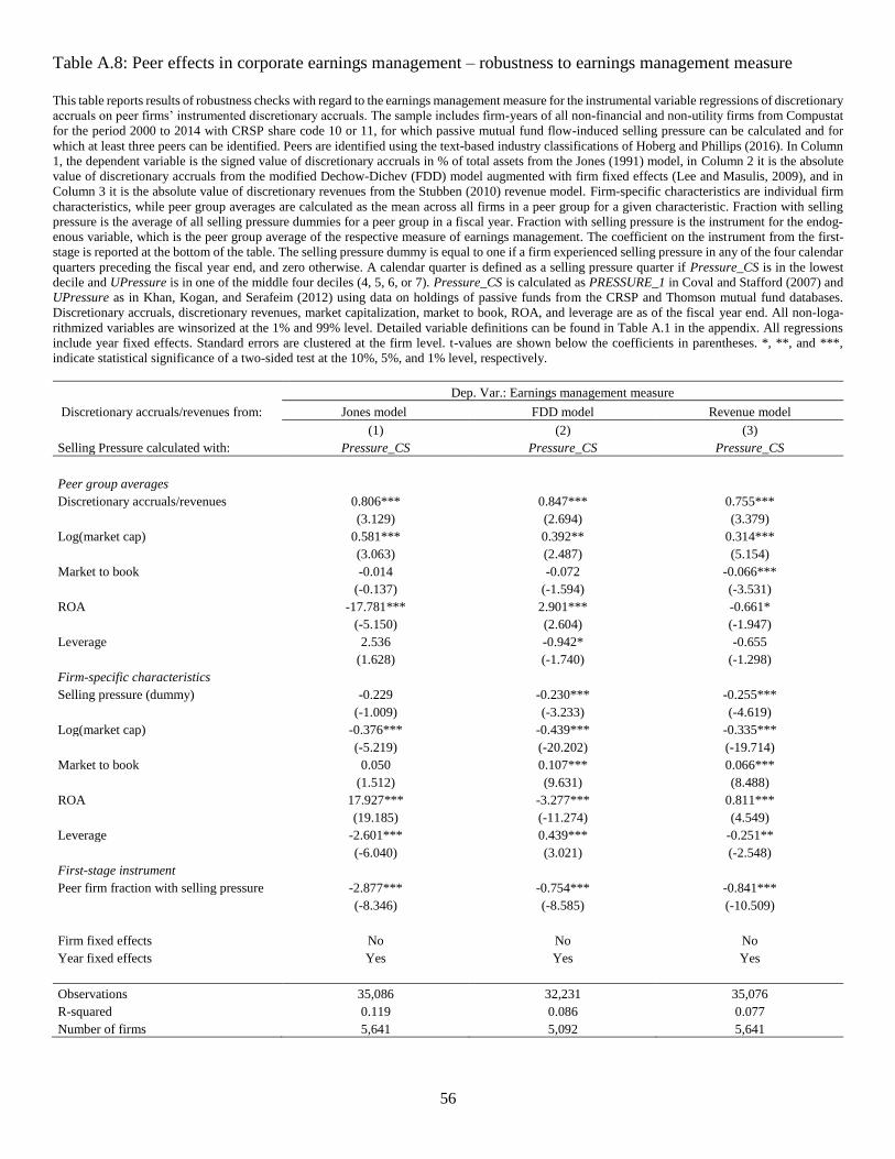
56

Table A.8: Peer effects in corporate earnings management – robustness to earnings management measure

This table reports results of robustness checks with regard to the earnings management measure for the instrumental variable regressions of discretionary

accruals on peer firms’ instrumented discretionary accruals. The sample includes firm-years of all non-financial and non-utility firms from Compustat

for the period 2000 to 2014 with CRSP share code 10 or 11, for which passive mutual fund flow-induced selling pressure can be calculated and for

which at least three peers can be identified. Peers are identified using the text-based industry classifications of Hoberg and Phillips (2016). In Column

1, the dependent variable is the signed value of discretionary accruals in % of total assets from the Jones (1991) model, in Column 2 it is the absolute

value of discretionary accruals from the modified Dechow-Dichev (FDD) model augmented with firm fixed effects (Lee and Masulis, 2009), and in

Column 3 it is the absolute value of discretionary revenues from the Stubben (2010) revenue model. Firm-specific characteristics are individual firm

characteristics, while peer group averages are calculated as the mean across all firms in a peer group for a given characteristic. Fraction with selling

pressure is the average of all selling pressure dummies for a peer group in a fiscal year. Fraction with selling pressure is the instrument for the endog-

enous variable, which is the peer group average of the respective measure of earnings management. The coefficient on the instrument from the first-

stage is reported at the bottom of the table. The selling pressure dummy is equal to one if a firm experienced selling pressure in any of the four calendar

quarters preceding the fiscal year end, and zero otherwise. A calendar quarter is defined as a selling pressure quarter if Pressure_CS is in the lowest

decile and UPressure is in one of the middle four deciles (4, 5, 6, or 7). Pressure_CS is calculated as PRESSURE_1 in Coval and Stafford (2007) and

UPressure as in Khan, Kogan, and Serafeim (2012) using data on holdings of passive funds from the CRSP and Thomson mutual fund databases.

Discretionary accruals, discretionary revenues, market capitalization, market to book, ROA, and leverage are as of the fiscal year end. All non-loga-

rithmized variables are winsorized at the 1% and 99% level. Detailed variable definitions can be found in Table A.1 in the appendix. All regressions

include year fixed effects. Standard errors are clustered at the firm level. t-values are shown below the coefficients in parentheses. *, **, and ***,

indicate statistical significance of a two-sided test at the 10%, 5%, and 1% level, respectively.

Dep. Var.: Earnings management measure

Discretionary accruals/revenues from: Jones model FDD model Revenue model

(1) (2) (3)

Selling Pressure calculated with: Pressure_CS Pressure_CS Pressure_CS

Peer group averages

Discretionary accruals/revenues 0.806*** 0.847*** 0.755***

(3.129) (2.694) (3.379)

Log(market cap) 0.581*** 0.392** 0.314***

(3.063) (2.487) (5.154)

Market to book -0.014 -0.072 -0.066***

(-0.137) (-1.594) (-3.531)

ROA -17.781*** 2.901*** -0.661*

(-5.150) (2.604) (-1.947)

Leverage 2.536 -0.942* -0.655

(1.628) (-1.740) (-1.298)

Firm-specific characteristics

Selling pressure (dummy) -0.229 -0.230*** -0.255***

(-1.009) (-3.233) (-4.619)

Log(market cap) -0.376*** -0.439*** -0.335***

(-5.219) (-20.202) (-19.714)

Market to book 0.050 0.107*** 0.066***

(1.512) (9.631) (8.488)

ROA 17.927*** -3.277*** 0.811***

(19.185) (-11.274) (4.549)

Leverage -2.601*** 0.439*** -0.251**

(-6.040) (3.021) (-2.548)

First-stage instrument

Peer firm fraction with selling pressure -2.877*** -0.754*** -0.841***

(-8.346) (-8.585) (-10.509)

Firm fixed effects No No No

Year fixed effects Yes Yes Yes

Observations 35,086 32,231 35,076

R-squared 0.119 0.086 0.077

Number of firms 5,641 5,092 5,641