Mathematical and Computational Applications, Vol. 10, No. 1, pp. 45-56, 2005. © Association for Scientific Research

PENALTY FUNCTION METHODS FOR CONSTRAINED OPTIMIZATION WITH GENETIC ALGORITHMS

Özgür Yeniay

Hacettepe University, Faculty of Science Department of Statistics, 06532,

Beytepe, Ankara yeniay@hacettepe.edu.tr

Abstract- Genetic Algorithms are most directly suited to unconstrained optimization. Application of Genetic Algorithms to constrained optimization problems is often a challenging effort. Several methods have been proposed for handling constraints. The most common method in Genetic Algorithms to handle constraints is to use penalty functions. In this paper, we present these penalty-based methods and discuss their strengths and weaknesses. Key Words- Genetic algorithms, Optimization, Constraint handling, Penalty function

1. INTRODUCTION Genetic Algorithms (GAs) are stochastic optimization methods based on concepts of natural selection and genetics [11,14]. They work with a population of individuals, each representing a possible solution to a given problem. GAs typically work by iteratively generating and evaluating individuals using an evaluation function. The simplest of GAs work according to the scheme shown in Figure 1. 1. Initialize population of individuals (t) 2. Evaluate each individual using evaluation function (t) 3. Repeat until a stopping criterion is satisfied

- Select parents from population (t) - Perform crossover on parents creating population (t+1) - Perform mutation on population (t+1) - Evaluate each individual of population (t+1)

Figure 1. The Steps of a Typical Genetic Algorithm They have been applied to a wide range of problems in diverse fields such as engineering, mathematics, operations research etc. (for a variety of applications, see [11,29]). Most of the problems in these fields are stated as constrained optimization problems. Since GAs are directly applicable only to unconstrained optimization, it is necessary to use some additional methods that will keep solutions in the feasible region. During the past few years, several methods were proposed for handling constraints by GAs [6,7,23,25,36]. Most of these methods have serious drawbacks. While some of them may give infeasible solution or require many additional parameters, others are problem-dependent (i.e. specific algorithm has to be designed for each particular problem). The most popular approach in GA community to handle constraints is to use

Ö. Yeniay 46

penalty functions that penalize infeasible solutions by reducing their fitness values in proportion to their degrees of constraint violation [30,36]. In this paper, we analyze these penalty-based methods. The rest of this paper is organized as follows. In the second section, a definition of a constrained optimization problem is given. The third section gives constraint handling methods and a classification of them. The fourth section provides an introduction to penalty functions and explains penalty-based methods in more detail. The last section concludes the paper.

2. CONSTRAINED OPTIMIZATION A constrained optimization problem is usually written as a nonlinear optimization problem of the following form:

m,...,1qj0)x(hq,...,1i0)x(g

tosubjectRSF)x,...,x(x)x(fMin

j

i

ntn1

+===≤

⊆⊆∈=

(1)

where t

n1 )x,...,x(x = is the vector of solutions, F is the feasible region and S is the whole search space. There are q inequality and m-q equality constraints. )x(f is usually called the objective function or criterion function. Objective function and constraints could be linear or nonlinear in the problem. Vector x that satisfies all the constraints is a feasible solution of the problem. All of the feasible solutions constitute the feasible region. Inequality constraints that satisfy 0)x(gi = are called active at x . Using these definitions, nonlinear programming problem is to find a point Fx* ∈ such that

)x(f)x(f * ≤ for all Fx∈ [3].

3. CONSTRAINT HANDLING in GAs There are several approaches proposed in GAs to handle constrained optimization problems. These approaches can be grouped in four major categories [28]: Category 1: Methods based on penalty functions

- Death Penalty [2] - Static Penalties [15,20] - Dynamic Penalties [16,17] - Annealing Penalties [5,24] - Adaptive Penalties [10,12,35,37] - Segregated GA [21] - Co-evolutionary Penalties [8]

Category 2: Methods based on a search of feasible solutions - Repairing unfeasible individuals [27] - Superiority of feasible points [9,32] - Behavioral memory [34]

Penalty Function Methods for Constrained Optimization 47

Category 3: Methods based on preserving feasibility of solutions - The GENOCOP system [26] - Searching the boundary of feasible region [33] - Homomorphous mapping [19]

Category 4: Hybrid methods [1,4,13,18,22] Note that there are other classification schemes of constraint handling methods in GAs. As seen above even though many methods to handle constrained optimization problems within GAs have been proposed this paper will concentrate on penalty function methods. 3.1. Penalty Functions Penalty method transforms constrained problem to unconstrained one in two ways. The first way is to use additive form as follows:

+∈

=otherwise),x(p)x(f

Fxif),x(f)x(eval (2)

where )x(p presents a penalty term. If no violation occurs, )x(p will be zero and positive otherwise. Under this conversion, the overall objective function now is )x(eval which serves as an evaluation function in GAs. Second way is to use multiplicative form,

∈

=otherwise),x(p)x(f

Fxif),x(f)x(eval (3)

For minimization problems, if no violation occurs )x(p is one and bigger than one, otherwise. The additive penalty type has received much more attention than the multiplicative type in the GA community. In classical optimization, two types of penalty function are commonly used: interior and exterior penalty functions. In GAs exterior penalty functions are used more than interior penalty functions. The main reason of this, there is no need to start with a feasible solution in exterior penalty functions. Because finding a feasible solution in many GAs problems is a NP- hard itself. The general formulation of an exterior penalty function is [7],

++=φ ∑∑

+==j

m

1qjji

q

1ii LcGr)x(f)x( (4)

Ö. Yeniay 48

where )x(φ indicates the new objective function to be optimized. Gi and Lj are the functions of )x(gi and )x(h j constraints respectively, and ri ve cj are penalty parameters. General formulas of Gi and Lj are,

[ ]β= )x(g,0maxG ii (5) γ

= )x(hL jj (6)

where β and γ are commonly 1 or 2. If the inequality is hold, 0)x(gi ≤ and [ ])x(g,0max i will be zero. Therefore the constraint does not effect )x(φ . If the

constraint is violated that means 0)x(gi > or 0h j ≠ , a big term will be added to )x(φ function such that the solution is pushed back towards to the feasible region. The severeness of the penalty depends on the penalty parameters ri and cj. If either the penalty is too large or too small, the problem could be very hard for GAs. A big penalty prevents to search unfeasible region. In this case GA will converge to a feasible solution very quickly even if it is far from the optimal. A pretty small penalty will cause to spend so much time in searching an unfeasible region; thus GA would converge an unfeasible solution [25]. Death Penalty This simple and popular method just rejects unfeasible solutions from the population: FSx,)x(P −∈+∞= . In this case, there will never be any unfeasible solutions in the population. If a feasible search space is convex or a reasonable part of the whole search space, it can be expected that this method can work well [30]. However, when the problem is highly constrained, the algorithm will spend a lot of time to find too few feasible solutions. Also, considering only the points that are in feasible region of the search space prevents to find better solutions. Static Penalties In the methods of this group, penalty parameters don’t depend on the current generation number and a constant penalty is applied to unfeasible solutions. Homaifar et al. [15] proposed a static penalty approach in which users describe some levels of violation. Steps of the method are as follows: • Generate l levels of violation for each constraint, • Generate penalty coefficient Rij (i=1,...,l ; j=1,…,m) for each level of violation and

each constraint. The bigger coefficients are given to the bigger violation levels, • Generate a random population using both feasible and unfeasible individuals, • Evaluate individuals using

[ ]2j

m

1jij )x(g,0maxR)x(f)x(eval ∑

=

+= (7)

where Rij indicates the penalty coefficient corresponding to jth constraint and ith violation level. m is the number of constraints. Homaifar et al. [15] transformed equality

Penalty Function Methods for Constrained Optimization 49

constraints to inequality constraints by 0)x(h j ≤ε− (where ε is a small positive number). The disadvantage of this method is the large number of parameters that must be set. In this method, for m constraints it is needed to set m(2l+1) parameters in total. For instance, for m=5 constraints and l=4 levels of violation the total of 45 parameters should be set. Michalewicz [31] shows that the quality of solutions is very sensitive to the values of these parameters. Kuri Morales and Quezada [20] suggested an another static penalty approach. In this method, individuals are evaluated using the following formula:

−

∈=

∑=

s

1iotherwise

mKK

Fxif),x(f)x(eval (8)

where s is the number of non-violated constraints and m is the total number of constraints. Constraints can be equality or inequality. K is a large positive constant. Kuri Morales and Quezada [20] used this constant as 1x109. There is only one restriction on K. K should guarantee that an unfeasible individual must be graded worse than a feasible individual. This approach uses information about the number of violated constraints, not the amount of constraint violation. Dynamic Penalties In the methods of this group, penalty parameters are usually dependent on the current generation number. Jones and Houck [16] suggested following dynamic function to evaluate individuals at each generation t:

)x,(SVC)tC()x(f)x(eval β+= α where C, α and β are constants determined by users. Joines and Houck [16] used C=0.5, α=1 or 2 and β=1 or 2. )x,(SVC β is described as

∑ ∑= +=

β +=βq

1i

m

1qjji )x(D)x(D)x,(SVC (9)

where

≤≤≤

=otherwise,)x(g

qi1,0)x(g,0)x(D

i

ii (10)

≤≤+ε≤≤ε−

=otherwise,)x(h

mj1q,)x(h,0)x(D

j

j

j (11)

Ö. Yeniay 50

This dynamic method increases the penalty as generation grows. The quality of a possible solution is very sensitive to changes of α and β values. There is no explanation about the sensitivity of the method for different values of C. Even Joines and Houck [16] stated that they used good selection of C=0.5 and α=β=2, Michalewicz [31] gave some examples to state that these parameter values cause premature convergence. He also showed that the method converges an unfeasible solution or a solution that is so far from an optimal solution. Kazarlis and Petridis [17] used the following dynamic penalty function,

sii

m

1ii B)))S(d(W(A)g(V)x(f)x(eval δ

+φδ+= ∑

=

(12)

where A=severity factor, m=total number of constraints,

=δotherwise,0

violatedisiconstraintif,1i

Wi= weight factor for constraint i, di(S)= measure of the degree of violation of constraint i introduced by solution S,

)S(iΦ = function of this measure, β= penalty threshold factor,

=δotherwise,0

feasibleisSif,1s

V(g)= an increasing function of the current generation g in the range (0,..,1). Kazarlis and Petridis [17] tried linear, quadratic and cubic forms of V(g) and received the best performance by

2

Gg)g(V

= (13)

where G is the total number of generations. This method needs some parameters depending on the problem. It is very hard to determine these parameters. Kazarlis and Petridis [17] did not state why they took A=1000 and B=0 in their work. Annealing Penalties There are some methods based on annealing algorithm in this group. Michalewicz and Attia [24] developed a method (GENECOP II) based on the idea of simulated annealing. Steps of this method are as follows: • Separate all constraints into four subsets: linear equations, linear inequalities,

nonlinear equations and nonlinear inequalities,

Penalty Function Methods for Constrained Optimization 51

• Find a random single point that satisfies linear constraints and take it as a starting point. The initial population consists of copies of this single point,

• Create a set of active constraints A which consists of nonlinear equations and violated nonlinear inequalities,

• Set τ=τ0, • Evolve the population using,

∑∈τ

+=τAj

2j )x(f

21)x(f),x(eval (14)

• If τ<τf (freezing point) stop the procedure, otherwise, - Diminish τ, - Use the best solution as a starting point for next generation, - Update A, - Repeat the previous step of the main part.

GENOCOP II distinguishes between linear and nonlinear constraints. In the algorithm only active constraints are under consideration at every iteration. While the temperature τ decrease, selective pressure on unfeasible solutions increases. As an interesting point of the method, there is no diversity of the initial generation that consists of multiple copies of a solution satisfied all linear constraints. At each generation the temperature τ decreases and the best solution found at the previous iteration is used as a starting point of next iteration. The algorithm is terminated at a previously determined freezing point τf . The method is very sensitive to values of the parameters. There is no specific way how to decide these parameters for any particular problem. Michalewicz and Attia [24] used τ0=1, τi+1=0.1τi and τf=0.000001 in their experiments. Carlson Skalak et al. [5] recommended to evaluate individuals using

)x(f)T,M()x(eval α= (15) In the formula, α(M,T) depends on the parameters M, the measurement of constraint violation, and temperature T, a function of running time of the algorithm. As execution proceeds, T approaches to zero. Carlson Skalak et al. [5] used the following function for α(M,T):

T/Me)T,M( −=α (16) Initial value of penalty parameter is small but increases over time so that unfeasible solutions found from last generations can be eliminated. For T,

t1T = (17)

is used. Here, t indicates the last temperature used at the previous iteration.

Ö. Yeniay 52

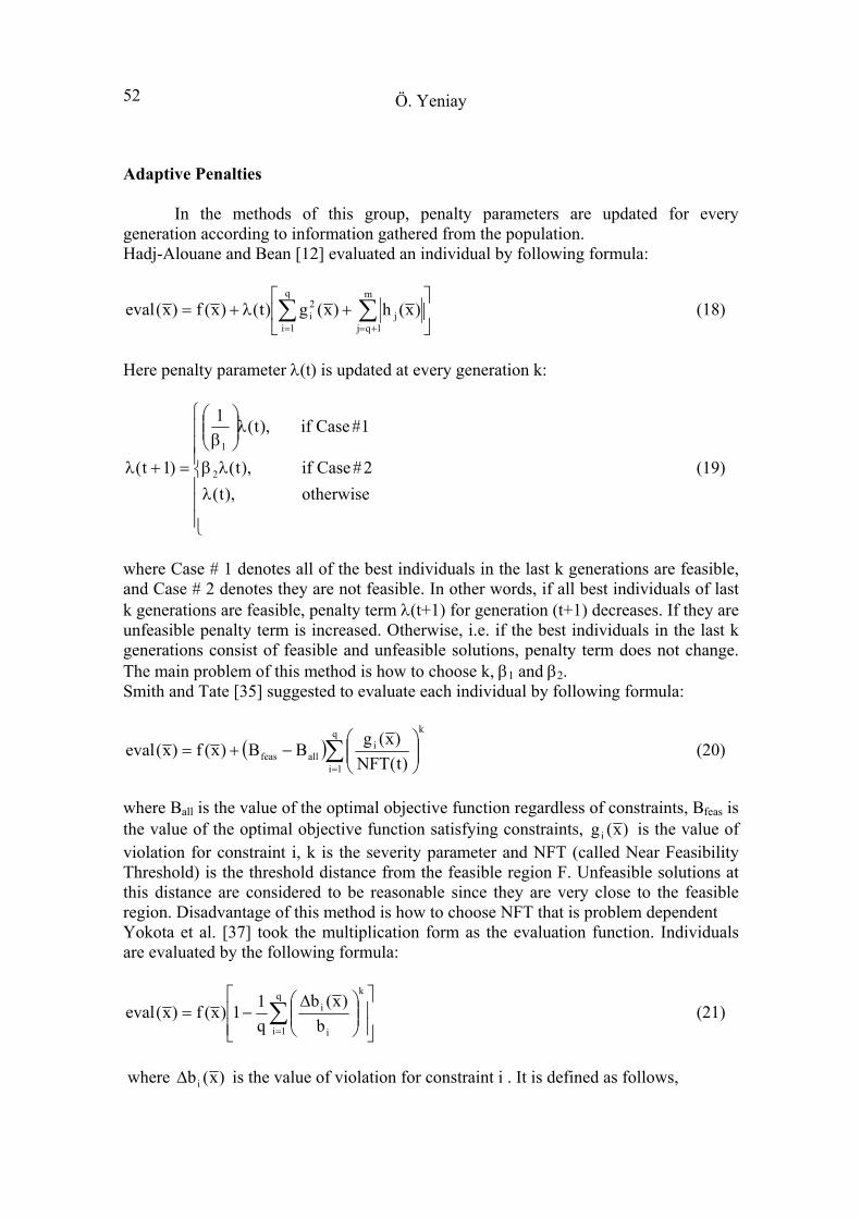
Adaptive Penalties In the methods of this group, penalty parameters are updated for every generation according to information gathered from the population. Hadj-Alouane and Bean [12] evaluated an individual by following formula:

+λ+= ∑ ∑

= +=

q

1i

m

1qjj

2i )x(h)x(g)t()x(f)x(eval (18)

Here penalty parameter λ(t) is updated at every generation k:

λλβ

λ

β

=+λotherwise),t(

2#Caseif),t(

1#Caseif),t(1

)1t( 2

1

(19)

where Case # 1 denotes all of the best individuals in the last k generations are feasible, and Case # 2 denotes they are not feasible. In other words, if all best individuals of last k generations are feasible, penalty term λ(t+1) for generation (t+1) decreases. If they are unfeasible penalty term is increased. Otherwise, i.e. if the best individuals in the last k generations consist of feasible and unfeasible solutions, penalty term does not change. The main problem of this method is how to choose k, β1 and β2. Smith and Tate [35] suggested to evaluate each individual by following formula:

( )∑=

−+=

q

1i

ki

allfeas )t(NFT)x(gBB)x(f)x(eval (20)

where Ball is the value of the optimal objective function regardless of constraints, Bfeas is the value of the optimal objective function satisfying constraints, )x(gi is the value of violation for constraint i, k is the severity parameter and NFT (called Near Feasibility Threshold) is the threshold distance from the feasible region F. Unfeasible solutions at this distance are considered to be reasonable since they are very close to the feasible region. Disadvantage of this method is how to choose NFT that is problem dependent Yokota et al. [37] took the multiplication form as the evaluation function. Individuals are evaluated by the following formula:

∆−= ∑

=

q

1i

k

i

i

b)x(b

q11)x(f)x(eval (21)

where )x(bi∆ is the value of violation for constraint i . It is defined as follows,

Penalty Function Methods for Constrained Optimization 53

[ ]iii b)x(g,0max)x(b −=∆ (22) For a feasible solution ii b)x(g ≤ is satisfied so for NFT=bi this approach is a special case of the approach of Smith and Tate [35]. Gen and Cheng [10] improved the approach presented above by giving high penalties for unfeasible solutions. Evaluation function is as follows:

∆∆

−= ∑=

q

1i

k

maxi

i

b)x(b

q11)x(f)x(eval (23)

In the formula above, )x(bi∆ is the value by which the constraint i is violated in the individual x . max

ib∆ is the maximum violation for constraint i among current population and ε is a small positive number. )x(bi∆ and max

ib∆ are defined as follows:

[ ]iii b)x(g,0max)x(b −=∆ (24)

[ ])t(Px;)x(b,maxb imaxi ∈∆ε=∆ (25)

The purpose of this method is to protect the diversity of the population and to protect the unfeasible solutions, which form the big part of the population in the early generations, from high penalties. Gen and Cheng [10] claims that their approach is independent from the problem. However, this approach is only used in an optimization problem so their claim can be appreciated as suspicious. Segregated GA Le Riche et al. [21] developed a segregated GA (sometimes it is called as yet another method) that uses two penalty parameters (say, p1 and p2) in two different populations. The aim is to overcome the problem of too high and too low penalties (see section 3.1). If a small value is selected for p1 and a large value for p2, a simultaneous convergence from feasible and unfeasible sides can be achieved. The method works as follows:

- Generate 2 x pop individuals at random (pop is the population size), - Design two different evaluation functions:

)x(p)x(f)x(f 11 += and )x(p)x(f)x(f 22 += - Evaluate each individual according to two evaluation functions, - Create two ranked lists according to )x(f1 and )x(f 2 , - Combine two ranked lists in a single one ranked population with size pop, - Apply genetic operators, - Evaluate the new population using both penalty parameters, - From the old and new populations generate two populations of the size pop each, - Repeat the last four steps of the process.

Ö. Yeniay 54

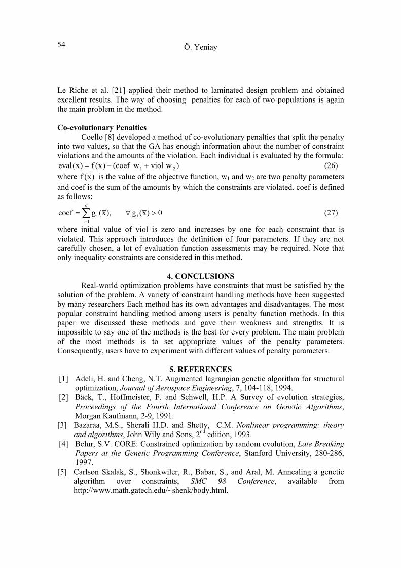
Le Riche et al. [21] applied their method to laminated design problem and obtained excellent results. The way of choosing penalties for each of two populations is again the main problem in the method. Co-evolutionary Penalties Coello [8] developed a method of co-evolutionary penalties that split the penalty into two values, so that the GA has enough information about the number of constraint violations and the amounts of the violation. Each individual is evaluated by the formula:

)wviolwcoef()x(f)x(eval 21 +−= (26) where )x(f is the value of the objective function, w1 and w2 are two penalty parameters and coef is the sum of the amounts by which the constraints are violated. coef is defined as follows:

0)x(g,)x(gcoef i

q

1ii >∀= ∑

=

(27)

where initial value of viol is zero and increases by one for each constraint that is violated. This approach introduces the definition of four parameters. If they are not carefully chosen, a lot of evaluation function assessments may be required. Note that only inequality constraints are considered in this method.

4. CONCLUSIONS Real-world optimization problems have constraints that must be satisfied by the solution of the problem. A variety of constraint handling methods have been suggested by many researchers Each method has its own advantages and disadvantages. The most popular constraint handling method among users is penalty function methods. In this paper we discussed these methods and gave their weakness and strengths. It is impossible to say one of the methods is the best for every problem. The main problem of the most methods is to set appropriate values of the penalty parameters. Consequently, users have to experiment with different values of penalty parameters.

5. REFERENCES [1] Adeli, H. and Cheng, N.T. Augmented lagrangian genetic algorithm for structural

optimization, Journal of Aerospace Engineering, 7, 104-118, 1994. [2] Bäck, T., Hoffmeister, F. and Schwell, H.P. A Survey of evolution strategies,

Proceedings of the Fourth International Conference on Genetic Algorithms, Morgan Kaufmann, 2-9, 1991.

[3] Bazaraa, M.S., Sherali H.D. and Shetty, C.M. Nonlinear programming: theory and algorithms, John Wily and Sons, 2nd edition, 1993.

[4] Belur, S.V. CORE: Constrained optimization by random evolution, Late Breaking Papers at the Genetic Programming Conference, Stanford University, 280-286, 1997.

[5] Carlson Skalak, S., Shonkwiler, R., Babar, S., and Aral, M. Annealing a genetic algorithm over constraints, SMC 98 Conference, available from http://www.math.gatech.edu/~shenk/body.html.

Penalty Function Methods for Constrained Optimization 55

[6] Coello, C.A.C. A Survey of constraint handling techniques used with evolutionary algorithms, Technical Report, Lania-RI-99-04, Laboratorio de Inform atica Avanzada, Veracruz, Mexico, 1999, available from http://www.cs.cinvestav.mx/~constraint/.

[7] Coello, C.A.C. Theoretical and numerical constraint-handling techniques used with evolutionary algorithms: A survey of the state of the art, Computer Methods in Applied Mechanics and Engineering, 191, 1245-1287, 2002.

[8] Coello, C.A.C. Use of a self-adaptive penalty approach for engineering optimization problems, Computers in Industry, 41, 113-127, 2000.

[9] Deb, K. An Efficient constraint handling method for genetic algorithms, Computer Methods in Applied Mechanics and Engineering, 186, 311-338, 2000.

[10] Gen, M. and Cheng, R. A Survey of penalty techniques in genetic algorithms, Proceedings of the 1996 International Conference on Evolutionary Computation, IEEE, 804-809, 1996.

[11] Goldberg, D.E. Genetic algorithms in search, optimization and machine learning, Addison-Wesley, Reading, MA, 1989.

[12] Hadj-Alouane, A.B. and Bean, J.C. A Genetic algorithm for the multiple-choice integer program, Operations Research, 45, 92-101, 1997.

[13] Hajela, P. and Lee, J. Constrained genetic search via schema adaptation, An immune network solution, Structural Optimization, 12, 11-15, 1996.

[14] Holland, J.H. Adaptation in naturel and artificial systems, MIT Press, Cambridge, 1975.

[15] Homaifar, A., Lai, S.H.Y. and Qi, X. Constrained optimization via genetic algorithms, Simulation, 62, 242-254, 1994.

[16] Joines, J. and Houck, C. On the use of non-stationary penalty functions to solve non-linear constrained optimization problems with GAs, Proceedings of the First IEEE International Conference on Evolutionary Computation, IEEE Press, 579-584, 1994.

[17] Kazarlis S. and V. Petridis, Varying fitness functions in genetic algorithms: studying the rate of increase in the dynamic penalty terms, Proceedings of the 5th International Conference on Parallel Problem Solving from Nature, Berlin, Springer Verlag, 211-220, 1998.

[18] Kim, J.H. and Myung, H. Evolutionary programming techniques for constrained optimization problems, IEEE Transaction on Evolutionary Computation, 1, 129-140, 1997.

[19] Koziel, S. and Michalewicz, Z. Evolutionary algorithms, homomorphous mapping and constrained parameter optimization, Evolutionary Computation, 7, 19-44, 1999.

[20] Kuri Morales, A. and Quezada, C.C. A Universal eclectic genetic algorithm for constrained optimization, Proceedings 6th European Congress on Intelligent Techniques & Soft Computing, EUFIT'98, 518-522, 1998.

[21] Le Riche, R., Knopf-Lenior, C. and Haftka, R.T. A Segregated genetic algorithm for constrained structural optimization, Proceedings of the Sixth International Conference on Genetic Algorithms, Morgan Kaufmann, 558-565, 1995.

Ö. Yeniay 56

[22] Le, T.V. Evolutionary approach to constrained optimization problems, Proceedings of the Second IEEE International Conference on Evolutionary Computation, IEEE Press, 274-278, 1995.

[23] Michalewicz, Z. A Survey of constraint handling techniques in evolutionary computation methods, Proceedings of the 4th Annual Conference on Evolutionary Programming, 135-155, 1995.

[24] Michalewicz, Z. and Attia, N. Evolutionary optimization of constrained problems, Proceedings of the Third Annual Conference on Evolutionary Programming, World Scientific, 98-108, 1994.

[25] Michalewicz, Z. and Fogel, D.B. How to solve it: Modern Heuristics, Springer Verlag, Berlin, 2000.

[26] Michalewicz, Z. and Janikow, C.Z. Handling constraints in genetic algorithms, Proceedings of the Fourth International Conference on Genetic Algorithms, Morgan Kaufmann, 151-157, 1993.

[27] Michalewicz, Z. and Nazhiyath, G. GENOCOP III: A Co-evolutionary algorithm for numerical optimization problems with nonlinear constraints, Proceedings of the Second IEEE International Conference on Evolutionary Computation, IEEE Press, 647-651, 1995.

[28] Michalewicz, Z. and Schouenauer, M. Evolutionary algorithms for constrained parameter optimization problems, Evolutionary Computation, 4, 1-32, 1996.

[29] Michalewicz, Z. Genetic algorithms + Data structures= Evolution programs, Second Edition, Springer Verlag, Berlin, 1994.

[30] Michalewicz, Z., Dasgupta, D., Le Riche, R. and Schoenauer, M. Evolutionary algorithms for constrained engineering problems, Computers & Industrial Engineering Journal, 30, 851-870, 1996.

[31] Michalewicz, Z. Genetic algorithms, numerical optimization, and constraints, Proceedings of the Sixth International Conference on Genetic Algorithms, Morgan Kaufmann, 151-158, 1995.

[32] Powell, D. and Skolnick, M.M. Using genetic algorithms in engineering design optimization with non-linear constraints, Proceedings of the Fifth International Conference on Genetic Algorithms, Morgan Kaufmann, 424-430, 1993.

[33] Schoenauer, M. and Michalewicz, Z. Evolutionary computation at the edge of feasibility, Proceedings of the Fourth International Conference on Parallel Problem Solving from Nature, Springer Verlag, 22-27, 1996.

[34] Schouenauer, M. and Xanthakis, S. Constrained GA optimization, Proceedings of the Fifth International Conference on Genetic Algorithms, Morgan Kaufmann, 473-580, 1993.

[35] Smith, A. and Tate, D. Genetic optimization using a penalty function, Proceedings of the fifth International Conference on Genetic Algorithms, Morgan Kaufmann, 499-503, 1993.

[36] Smith, A.E. and Coit, D.W. Constraint handling techniques- penalty functions, Handbook of Evolutionary Computation, chapter C 5.2. Oxford University Press and Institute of Physics Publishing, 1997.

[37] Yokota, T., Gen, M., Ida, K. and Taguchi, T. Optimal design of system reliability by an improved genetic algorithm, Electron. Commun. Jpn. 3, Fundam. Electron. Sci.79, 41-51,1996.