pension risk management with funding and … risk... · pension risk management with funding and...
TRANSCRIPT

PENSION RISK MANAGEMENT WITH FUNDING AND BUYOUT OPTIONS
ABSTRACT
There has been a surge of interest in recent years from defined benefit pension plan
sponsors in de-risking their plans with strategies such as “longevity hedges” and “pen-
sion buyouts” (Lin et al., 2015). While buyouts are attractive in terms of value cre-
ation, they are capital intensive and expensive, particularly for firms with underfunded
plans. The existing literature mainly focuses on the costs and benefits of pension buy-
outs. Little attention has been paid to how to capture the benefits of de-risking within
a plan’s financial means, especially when buyout deficits are significant. To fill this
gap, we propose two options, namely a pension funding option and pension buyout
option, that provide financing for both underfunded and well funded plans to cover the
buyout risk premium and the pension funding deficit, if a certain threshold is reached.
To increase market liquidity, we create a transparent pension funding index, calcu-
lated from observed capital market indices and publicly available mortality tables, to
determine option payoffs. A simulation based pricing framework is then introduced to
determine the prices of the proposed pension options. Our numerical examples show
that these options are effective and economically affordable. Moreover, our sensitivity
analyses demonstrate the reliability of our pricing models.
Keywords: defined benefit pension plan, risk management, pricing, funding options,
buyout options.
Date: November 30, 2015.1

2 PENSION RISK MANAGEMENT WITH FUNDING AND BUYOUT OPTIONS
1. INTRODUCTION
A parade of bad news, from unprecedented market swings to sustained declines in interest rates,
has caused double-digit losses of many defined benefit (DB) plan sponsors in several years of the last
decade. Unanticipated improvements in mortality rates increase pension liabilities (Cox et al. (2006);
Cox and Lin (2007); Lin and Cox (2008); Cox et al. (2010); Milidonis et al. (2011); Cox et al. (2013);
Lin et al. (2013)). While the investment experience was favorable in 2014, due to a decline in interest
rates, it was not enough to offset pension liability increases. In January 2015, the Milliman 100
Pension Funding Index (PFI) decreased to 79.6%, down from 83.5% in December 2014 (Milliman,
2015). The PFI is based on the 100 largest corporate DB pension plans in the Unites States. Pension
funding deficits increase volatilities of corporate earnings, balance sheets, and cash flows and reduce
share value (Bunkley, 2012). As a result, there has been a surge of interest from DB plan sponsors
to de-risk their pensions with strategies such as longevity hedges and pension buyouts in recent years
(Lin et al., 2015). A longevity hedge, such as a longevity swap, allows a pension plan to transfer its
high-end longevity risk to a third party. In contrast, a pension buyout involves purchasing annuities
from an insurance company. A buyout allows a firm to offload all pension liabilities from its balance
sheet.
Compared with longevity hedges, pension buyouts are more effective in improving firm value.
Longevity hedges only transfer extreme longevity risk and retain most of pension risk, so they prevent
a firm from taking full advantage of pension de-risking. Pension buyouts, on the other hand, transfer
the entire pension risk including investment risk, interest rate risk and longevity risk. Thus, pension
buyouts provide more freedom for a firm, within its risk tolerance, to take on more risky projects with
high positive net present values. Consistent with this observation, Lin et al. (2015) find that in the
enterprise risk management framework, buyouts create more value than longevity hedges.1
While buyouts are attractive in terms of value creation, they are capital intensive and relatively
expensive. Mercer uses up-to-date pricing information to estimate the approximate costs of pension
buyouts in four countries: U.S., U.K., Ireland and Canada. In December 2014, the price of a buyout
1Enterprise risk management (ERM) assesses all enterprise risks and coordinates various risk management strategies in aholistic way (Lin et al., 2015). ERM is likely to create value because it integrates all risk factors and ensures individualdecisions handling idiosyncratic risks compatible with a firm’s overall risk appetite and global corporate agenda (Lam,2001; Liebenberg and Hoyt, 2003; Nocco and Stulz, 2006).

PENSION RISK MANAGEMENT WITH FUNDING AND BUYOUT OPTIONS 3
annuity transaction across these four countries was 14% higher on average than the equivalent ac-
counting liability (i.e. projected benefit obligation (PBO)) based on FASB Accounting Standard ASC
715 (Mercer LLC, 2014). This buyout cost estimate is based on the assumption that a plan consists
of retirees only with a duration of nine years. In fact, the actual cost of a buyout could be higher.
If predicted mortality rates are higher than assumed ones used to measure the balance sheet value of
pension obligations and/or capital markets deteriorate in the future, annuity insurers will likely require
a higher buyout price to cover pension risk.
In addition to high upfront annuity premiums, buyouts can be very expensive for firms with under-
funded plans. To complete buyout transactions, these firms have to satisfy a minimum funded status
by infusing cash to cover their funding deficits. In practice, pension shortfalls should be paid imme-
diately or over an amortization period with a series of regular payments. Recent falling interest rates
and subdued equity markets have driven up buy-out deficits of most pension plans. Thus, while many
firms would like to de-risk their pensions through buy-outs, due to the high cost at present, it is not
a good idea to use shareholder funds to finance buyout deals (LCP, 2012, page 6). This may explain
why longevity swaps generally have had higher business volume than buyouts in recent years, even
though buyouts can create greater value.
Lane Clark & Peacock LLP, a leading pension consulting firm, argues that we should explore
well-designed structures that make buyouts easier for underfunded plans (LCP, 2012). Nevertheless,
with only a few exceptions, cost effective strategies that make buyouts affordable have been largely
unexplored. The existing literature focuses mainly on costs and benefits of pension buyouts (Cox
et al., 2013; Lin et al., 2014, 2015). Little attention has been paid to how to capture the benefits of
this de-risking option within a plan’s financial means, especially when buyout deficits are significant.
To fill this gap, we first investigate innovative ways to achieve pension buyouts for underfunded DB
plans in a value-enhancing way.
Specifically, we propose two types of options that provide financing to underfunded plans if a
pension funding index improves to a certain level. This certain level, called the trigger level, is set
at a ratio less than the fully funded ratio 100%. To increase market liquidity, we create a transparent
pension funding index to determine option payoffs. This pension funding index, to be explained in
detail in a later section, is calculated from observed capital market indices and publicly available

4 PENSION RISK MANAGEMENT WITH FUNDING AND BUYOUT OPTIONS
mortality tables. Our first proposed option, the pension funding option, provides a payoff equal to
the difference between a strike funding level and the pension funding index if the option is triggered.
The second pension option, the pension buyout option, provides a payoff to cover the buyout risk
premium and pension funding deficit if the pension funding index reaches a threshold. In reality,
there is a misconception among pension sponsors that pension risk can be transferred only if a plan
is well funded (Mathur and Kaplan, 2013). Indeed, our proposed options provide an innovative and
promising venue for severely underfunded firms to execute buyouts before they reach full funding.
The moral hazard and adverse selection problem is low in our setup because these options will pay
out only if the index is triggered, irrespective of the actual pension performance of option buyers.
While these options are index-based, basis risk may not be a serious concern because our proposed
pension funding index can be flexibly designed to resemble the funding dynamics of a particular
pension plan.
On the other hand, some firms with well funded DB plans are currently reluctant to adopt buyouts
because they are comfortable with retaining market risk or they may feel the buyout annuity price
is too high (Mathur and Kaplan, 2013). Regulation and legal issues related to buyout transactions
further deter DB plan sponsors from shedding their pension obligations now. For example, Verizon
retirees sued Verizon and challenged its buyout deal with Prudential that annuitized benefits of 41,000
retirees. While the claims were dismissed, Verizon retirees continued their fight in court. This lawsuit
may stir a change in pension law (Buckmann, 2014). For example, the ERISA advisory council is
considering new rules for buyouts. The possibility of changes to the law, therefore, may be another
reason why fully funded pension firms hesitate to implement buyouts. If new laws on de-risking
transactions remove ambiguities and disputes, we expect more pension sponsors to take actions to
transfer their pension liabilities, especially when their DB pensions start to cause problems. The
difficulty is that, at that time their funding status deteriorates, the cost of buyouts may be high due to
large plan deficits. Therefore, we propose two more pension funding and buyout options that allow
a currently well-funded firm to exercise the option and use the option payoff to fund their buyouts
in the future, when the pension funding index falls below a given level. That is, the options provide
funding for pension sponsors when they are highly motivated to remove their pension liabilities from
their balance sheets.

PENSION RISK MANAGEMENT WITH FUNDING AND BUYOUT OPTIONS 5
A market for these options will develop if they are effective, economically affordable, and trans-
parently priced. Thus, as the second objective of this paper, we show how to explicitly price these
options. We first model the evolution of the pension funding index as the ratio of a flexibly designed
pension asset index to a pension liability index. The pension asset index is calculated from several
market indices based on predetermined investment weights, while the pension liability index is eval-
uated using a publicly available projected mortality table estimated with the Lee and Carter (1992)
mortality model. The payoffs of pension funding options depend on the relation between a strike
funding ratio and the pension funding index. If these pension options are only exercisable on valua-
tion dates, they can be decomposed to a series of single period European “gap-type” options.2 We use
Monte Carlo simulation to obtain the payoffs and risk neutral prices for pension funding options. Un-
like pension funding options, pension buyout options include an immediate buy-out feature when the
funding threshold is triggered. We account for this pension take-over feature to properly price these
options. Specifically, at the time the option is exercised, the payoff has a buyout risk premium, which
can be evaluated using the approach introduced by Lin et al. (2015). The same pricing framework for
funding options can be applied to buyout options with modified option payoffs.
This work contributes to the growing body of research on pension de-risking in three ways. First,
this paper adds to the pension risk management literature by proposing new ways to reduce pension
risk. Some plan sponsors view transferring DB risk to an insurer as too expensive. Our proposed
options aim to fill the gap between the intentions and actions of pension sponsors with respect to
pension risk transfer with buyouts. They provide a cost effective way to address pension risk, making
buyouts feasible for underfunded pension firms and cheaper for well-funded firms that decide to defer
their buyout decisions. Second, to increase market liquidity and reduce moral hazard and adverse
selection problems, we introduce a transparent pension funding index based on market indices and
publicly available mortality tables. It will lower transaction costs and help develop pension option
markets. Third, we contribute to the existing studies on pension risk pricing. We show how to price
these new pension de-risking securities while recognizing investment risk, longevity risk, and interest
2McDonald (2013, page 422) discusses gap options. There are pricing formulas for gap options in the Black-Scholessetting.

6 PENSION RISK MANAGEMENT WITH FUNDING AND BUYOUT OPTIONS
rate risk. Moreover, we propose how to incorporate buyout risk premiums for pricing pension buyout
options.
2. SECURITIZATION OF PENSION RISK WITH OPTIONS
Pension buyouts, a pension de-risking strategy, have gained more and more attention from both
scholars and practitioners. To facilitate development of this emerging market, we propose financial
innovations that provide new venues to reduce pension risk exposures and make buyouts more afford-
able to pension sponsors. In a later section, we will show how to price these securities.
2.1. Pension Funding Index. Index-based securitization reduces moral hazard and adverse selec-
tion, increases liquidity, reduces transaction costs, and provides a standardized and transparent struc-
ture. Thus, our proposed pension options are based on a pension funding index calculated from
various market indices and publicly available mortality tables. Specifically, the pension funding index
at time t, PFIt, is defined as the ratio of a pension asset index PAIt to a pension liability index PLIt:
PFIt =PAItPLIt
. (1)
The pension liability index is based on a retired life cohort with N(0) members of age x0 at time
0. The number of lives N(0) and the age x0 may depend on a particular plan under consideration
for a funding or buyout option.3 To ensure transparency, when calculating the pension liability index
PLIt at time t, we use a publicly available population mortality table based on the projected future
mortality rates. Assume that each surviving member of the cohort receives an annual survival benefit
of P , paid at the end of each year. For a given plan, we can use the average annual benefit for the
members of the cohort of N(0) at time t = 0. Then PLIt is the present value at time t of all future
benefit payments to N (t) surviving retirees at time t:
PLIt = N(t) · Pax0+t t = 1, 2, · · · . (2)
At time t = 0, the number of retirees, N(0), and the annual payment, P , are known. Thus at time
0, PLI0 is known: PLI0 = N(0) · Pax0 . In (2), ax0+t is the immediate life annuity factor for age
3The group of retirees under consideration may have different ages at time t = 0. We can easily adjust the model if that isthe case. The main thing is that the ages and number of retirees at each age are known at time t = 0.

PENSION RISK MANAGEMENT WITH FUNDING AND BUYOUT OPTIONS 7
x = x0 + t given the predicted mortality rates at time t:
ax = ax0+t =∞∑s=1
vst spx,t, (3)
where vt = 1/(1 + rp,t) is the discount factor based on the pension valuation rate rp,t. The conditional
expected s-year survival rate for age x at time t, spx,t, is calculated as:
spx,t = E [spx,t |px,t, px+1,t+1, · · · , px+s−1,t+s−1 ] , (4)
where px+s−1,t+s−1, s = 1, 2, · · · is the probability that a plan member at age x + s − 1 at time
t+ s− 1 survives to age x+ s at the beginning of year t+ s, based on a forecasted mortality table at
time t+ s− 1.
The pension asset index PAIt is determined by the value of a market portfolio composed of I
indices at time t. That is,
PAIt =I∑i=1
Ai,t−1(1 + ri,t), i = 1, 2, · · · , I; t = 1, 2, · · · , (5)
where Ai,t−1 is the amount invested in index i at time t − 1 and ri,t is the return of index i in period
t. At time 0, PAI0 is set at a predetermined value denoted PA0 with Ai,0 = wiPA0 where wi is the
weight of index i that represents a plan’s typical weight in that asset category. That is, the initial fund
amount PA0 and the weights wi can be tailored to a specific plan under consideration for a funding
or buyout option. Given N(t) survivors at time t, the following relation holds:
PAt =I∑i=1
Ai,t
= PAIt + kt · ULt · 1{ULt>0} −N(t)P, t = 1, 2, · · · ,
where ULt is the funding deficit measured as
ULt = PLIt − PAIt +N(t)P, t = 1, 2, · · · . (6)

8 PENSION RISK MANAGEMENT WITH FUNDING AND BUYOUT OPTIONS
Following Maurer et al. (2009) and Cox et al. (2013), the pension underfunding amortization factor
kt is equal to
kt =1∑m−1
i=0 (1 + rp,t)−i, (7)
wherem > 1 is the number of years of the amortization period. At the end of each period, the pension
fund PAt is rebalanced so that the weight invested in index i stays at wi, i = 1, 2, · · · , I . That is,
Ai,t = wi · PAt = wi(PAIt + kt · ULt · 1{ULt>0} −N(t)P
), (8)
where∑I
i=1wi = 1. With this setup, the evolution of the pension asset index PAIt will closely
resemble the dynamics of a typical pension plan’s asset portfolio.
2.2. Pension Options. We propose several pension options for fully funded plans as well as under-
funded plans, based on the pension funding index PFIt.
2.2.1. Pension Options for Fully Funded Plans. Some well-funded pension sponsors choose not to
execute pension buyouts (Mathur and Kaplan, 2013). However, a fully funded plan may want to obtain
the right to a buyout in the future, if its funding deteriorates. Future asset values may be volatile and
future liabilities may increase due to improving mortality of retirees. A plan can become underfunded
and require cash injection in the future, in which case implementing a pension buyout may become
very expensive. Thus, we propose a pension funding option that allows a plan to retain the option to
execute a buyout, in the face of future underfunding. This option preserves flexibility to finance future
buyouts at a low cost.
Consider a pension plan that is fully funded at time 0. Suppose its funding status is highly correlated
with the pension funding index PFIt. To manage its pension funding risk, the plan can purchase the
following n-year funding option with a strike funding level K. The option is defined in terms of a
notional amount, NA, the trigger funding index level, z, at which the option may be exercised, the
strike level, K > z, and the option term n. It may be exercised at time t = 1, 2, . . . , n but only if
PFIt < z. The payoff at time t is summarized as follows:
Fwt =
NA
PLI0×
PLIt (K − PFIt) if PFIt < z
0 if PFIt ≥ z
, for t = 1, 2, . . . , n. (9)

PENSION RISK MANAGEMENT WITH FUNDING AND BUYOUT OPTIONS 9
PFIt, as described in (1), is the pension funding index at time t = 1, 2, . . . , n. With this option,4
if the PFIt falls below the trigger z, the plan may exercise the option and receive a payoff equal to
NAPLItPLI0
(K−PFIt). The term PLItPLI0
measures the remaining percentage of pension liabilities at time
t as the number of surviving retirees in the plan declines overtime. The payoff allows the plan to make
up its funding deficits and reduce costly external financing to complete the buyout transaction.
This funding option provides cash to the DB sponsor to cover a future funding deficit and satisfy
a minimum funding requirement for a future buyout. However, the cash may not be sufficient to pay
the full cost of a buyout, if the strike level K is less than or equal to the full funding ratio 100%.
Additional cash may be required to complete the buyout. The buyout price, in general, is higher than
the expected pension liabilities because buyout insurers require a risk premium. For example, recent
UK buyout prices were about 14% above the value of pension liabilities covered.
We define a second option which recognizes the buyout provider’s risk premium, as follows, with
the same definitions of the trigger point z, strike level K, and term n. This buyout option provides a
currently fully funded plan with the following payoff at time t:
Bwt =
NA
PLI0×
PLIt (K − PFIt +Rt) if PFIt < z
0 if PFIt ≥ z
, (10)
where Rt is the estimated buyout risk premium at time t. This buyout option has a higher payoff than
the funding option in (9). Accordingly, the buyout option will have a higher price than the funding
option.
2.2.2. Pension Options for Under-Funded Plans. In contrast to a fully funded pension plan, an un-
derfunded plan may not have the cash for a buy-out immediately, even though the plan sponsor may
want a buyout. To make the pension buyout feasible, such a plan can purchase a n-year funding option
with a strike level K and a notional amount of NA, subject to a trigger PFIt > z where z < K. The
4In option terminology, this is an n-year Bermudian gap put option written on the pension funding index.

10 PENSION RISK MANAGEMENT WITH FUNDING AND BUYOUT OPTIONS
following expression describes the value of this option at time t:
F ut =
NA
PLI0×
0 if PFIt ≥ K
PLIt (K − PFIt) if z < PFIt < K
0 if PFIt ≤ z
for t = 1, 2, . . . , n. (11)
If the funding index PFIt improves and exceeds the trigger z, but less than the strike K at time t,
the option will be exercised, providing a payoff of NAPLItPLI0
(K − PFI0). To avoid a negative option
payoff, in (11), we set the payoff equal to 0 if PFIt ≥ K. As long as the funding status of the plan
is highly correlated with the pension funding index PFIt, the payoff from the option makes it easier
for the plan to pay for a buyout.
An underfunded firm may want to enter a buyout transaction right after its funding ratio reaches z.
As in the case of a fully funded plan, we introduce a buyout option that recognizes the provider’s risk
premium. For such an underfunded plan, the buyout option payoff But at time t is defined as follows:
But =
NA
PLI0×
PLIt ×Rt if PFIt ≥ K
PLIt (K − PFIt +Rt) if z < PFIt < K
0 if PFIt ≤ z
. (12)
The pension funding index PFIt can be designed initially to track a plan’s funding dynamics. Then,
the payoff from this buyout option will very likely pay the entire buyout annuity premium for the
underfunded plan.
2.3. Discussion. In the UK, pension plan deal volume in 2013 included £8.9 billion of longevity
swaps and £7.45 billion of bulk annuity buyouts (Ward, 2014). The reinsurers and insurers providing
these transfers might very well be interested in developing and including buyout options to expand the
range of their provided risk management tools. The actuarial consulting firms currently advising plan
sponsors could assist in obtaining appropriate pension buyout options. As we documented earlier,
the interest from plan sponsors in managing pension risks is substantial. The demand for buyouts
in the U.S. increases because “increasing PBGC premiums and increasing longevity” are making
it harder for pension plan sponsors to maintain DB plans (Ebling, 2014). While many plans have

PENSION RISK MANAGEMENT WITH FUNDING AND BUYOUT OPTIONS 11
recovered from the 2008 crisis, the remaining under-funded plans may see buyout options as a means
to eventually transfer unwanted risks. Importantly, these options allow plans that are not eligible for
a traditional buyout to execute buyouts easier. In sum, it seems reasonable that buyout options will be
attractive to a significant number of sponsors. Moreover, it appears feasible for the current providers
of mortality swaps and buyouts to arrange buyout options to accompany their existing buyout and
mortality swap products.
3. BASIC FRAMEWORK
3.1. Pension Asset Index. Suppose the pension asset index PAIt is composed of three indexes at
time t: the S&P 500 index (i = 1), the Merrill Lynch corporate bond index (i = 2), and the 3-month
T-bill index (i = 3) with the weights of w1, w2 and w3. Under the physical (P) risk measure, the
process of the S&P 500 index at time t, A1,t, is described by the following stochastic differential
equation (SDE):
dA1,t
A1,t−= (α1 − λ1k1) dt+ σ1 dW P
1t + d
(N1t∑j=1
(V1j − 1)
), (13)
where α1 is the instantaneous expected return and σ1 is the instantaneous volatility of the S&P 500
index. The standard Brownian motion W P1t has a mean 0 and variance t. The Poisson process N1t
has a mean number of arrivals λ1 per unit of time. The independently and identically distributed
jump size V1j for j = 1, 2 . . . is modeled as a lognormal random variable (Merton, 1976). Thus, its
logarithm Y1j = log V1j is a standard normal random variable with mean m1 and standard deviation
s1. A Poisson event will cause an expected percentage change in the S&P 500 index equal to k1 ≡
E(V1j − 1). Solving the SDE (13) provides an explicit expression for the S&P 500 index process:
A1,t = A1,0 exp [Xt] = A1,0 exp
[(α1 −
1
2σ21 − λ1k1)t+ σ1W
P1t +
N1t∑j=1
Y1j
]. (14)
Due to the market incompleteness introduced by the jump-diffusion process (14), we are no longer
able to find a unique risk-neutral (martingale equivalent) measure. The transition from the physical
world to the risk neutral world varies, depending on which type of distance minimization is selected.
To preserve the same kind of jump-diffusion framework under measure change, we follow Gerber and

12 PENSION RISK MANAGEMENT WITH FUNDING AND BUYOUT OPTIONS
Shiu (1994) and adopt an Esscher transform of the logarithmic asset return as our martingale equiv-
alent measure. It can be shown that such a risk neutral measure is the closest martingale equivalent
measure to the physical measure in terms of a power utility function (Gerber and Shiu, 1994, p.175-
177). Define the risk neutral Esscher measure P ∗(Xt, h) through its corresponding Radon-Nikodym
derivative: (dP ∗
dP
)∣∣∣∣Ft
=ehXt
E [ehXt ], (15)
where h is a real constant such that E[ehXt
]exists.
Under the risk neutral Esscher measure P ∗(Xt, h), the process of the S&P 500 index, A1,t, still
follows a Merton-type jump-diffusion process:
A1,t = A1,0 exp
(r − 1
2σ21 − λ∗1k∗1
)t+ σ1W
P ∗
1t +
N∗1t∑
j=1
Y ∗1j
, (16)
where r is the risk-free interest rate, W P ∗1t = W P
1t − hσ1t is a standard Brownian motion under P ∗,
and the new Poisson and jump size parameters are
λ∗1 = λ1 exp
(m1h+
1
2s21h
2
), m∗1 = m1 + s21h, (17)
with the standard deviation s∗1 = s1 unchanged. The parameter h is determined such that {e−rtA1,t, t ≥ 0}
is a martingale with respect to the Esscher risk measure P ∗. More specifically, the parameter h satis-
fies
α1 − λ1k1 + σ21h+ λ∗1k
∗1 = r (18)
(see, e.g. Bo et al. (2010)). Such explicit analytic relations among the parameters under the physical
risk measure and the risk neutral Esscher measure provide significant convenience for the numerical
illustrations in Section 5.

PENSION RISK MANAGEMENT WITH FUNDING AND BUYOUT OPTIONS 13
The dynamic processes of the Merrill Lynch corporate bond index (i = 2) and the 3-month T-bill
index (i = 3) are modeled as geometric Brownian motions:5
dAi,tAi,t
= αi dt+ σi dWPit , i = 2, 3 (19)
in the physical risk world and
dAi,tAi,t
= r dt+ σi dWQit , i = 2, 3 (20)
in the risk neutral (Q) world, where the constant α2 (α3) is the drift of the Merrill Lynch corporate
bond index (the 3-month T-bill index) with an instantaneous volatility σ2 (σ3). In (19) and (20),
W Pit (WQ
it ) is a standard Brownian motion with mean 0 and variance t. The correlation between the
standard Brownian motions W P1t (W P ∗
1t ) and W P2t (WQ
2t ) is denoted as ρ.6
3.2. Dynamic Pension Valuation Rate. The value of pension liabilities is closely related to the yield
of long-term corporate bonds, which implies that considerable attention should be paid to the interest
rate risk in pension risk management. Although long-term interest rates are far less volatile than
short-term rates, the U.S. composite corporate bond rates7 published by the Internal Revenue Service
(IRS) do show some smooth changes from time to time. As pointed out by Gukaynak et al. (2005),
“long-term forward rates move significantly in response to many macroeconomic data releases and
monetary policy announcements”. Consequently, it is of great importance to incorporate the dynamics
of pension valuation rate into the pricing framework of pension options. While there exist a variety of
short-term interest rate models in the literature (to name only a few, Cox et al. (1985); Hull and White
(1990); Longstaff and Schwartz (1992)), few simple and effective models have been proposed to
capture the movement of long-term interest rates. In this paper, we cautiously use the Cox-Ingersoll-
Ross (CIR) model (Cox et al., 1985) to illustrate the dynamics of the pension valuation rate. That is,
the pension valuation rate rp,t satisfies the following process:
drp,t = ν (θ − rp,t) dt+ σp√rp,t dW P
p,t, (21)
5Our statistical test rejects the model with a jump for the processes of the Merrill Lynch corporate bond index and the3-month T-bill index based on the monthly data from March 1988 to December 2010.6We reject a significant correlation between WP
1t and WP3t as well as between WP
2t and WP3t in our sample period.
7https://www.irs.gov/Retirement-Plans/Composite-Corporate-Bond-Rate-Table.
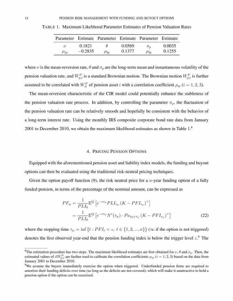
14 PENSION RISK MANAGEMENT WITH FUNDING AND BUYOUT OPTIONS
TABLE 1. Maximum Likelihood Parameter Estimates of Pension Valuation Rates
Parameter Estimate Parameter Estimate Parameter Estimate
ν 0.1821 θ 0.0569 σp 0.0035ρ1p −0.2835 ρ2p 0.1377 ρ3p 0.1255
where ν is the mean-reversion rate, θ and σp are the long-term mean and instantaneous volatility of the
pension valuation rate, and W Pp,t is a standard Brownian motion. The Brownian motion W P
p,t is further
assumed to be correlated with W Pit of pension asset i with a correlation coefficient ρip (i = 1, 2, 3).
The mean-reversion characteristic of the CIR model could potentially enhance the stableness of
the pension valuation rate process. In addition, by controlling the parameter σp, the fluctuation of
the pension valuation rate can be relatively smooth and hopefully be consistent with the behavior of
a long-term interest rate. Using the monthly IRS composite corporate bond rate data from January
2001 to December 2010, we obtain the maximum likelihood estimates as shown in Table 1.8
4. PRICING PENSION OPTIONS
Equipped with the aforementioned pension asset and liability index models, the funding and buyout
options can then be evaluated using the traditional risk-neutral pricing techniques.
Given the option payoff function (9), the risk neutral price for a n-year funding option of a fully
funded pension, in terms of the percentage of the nominal amount, can be expressed as
PFw =1
PLI0EQ[e−rτwPLIτw (K − PFIτw)+
]=
1
PLI0EQ[e−rτwN∗(τw) · Pax0+τw (K − PFIτw)+
](22)
where the stopping time τw = inf {t : PFIt < z, t ∈ {1, 2, ..., n}} (∞ if the option is not triggered)
denotes the first observed year-end that the pension funding index is below the trigger level z.9 The
8The estimation procedure has two steps. The maximum likelihood estimates are first obtained for ν, θ and σp. Then, theestimated values of dWP
p,t are further used to calibrate the correlation coefficients ρip (i = 1, 2, 3) based on the data fromJanuary 2001 to December 2010.9We assume the buyers immediately exercise the option when triggered. Underfunded pension firms are required toamortize their funding deficits over time (as long as the deficits are not covered), which will make it unattractive to hold apension option if the option can be exercised.

PENSION RISK MANAGEMENT WITH FUNDING AND BUYOUT OPTIONS 15
survival evolution of the pension cohort N∗(t) (and thus, PFIt) in (22) is based on the transformed
mortality rates to reflect the market expectation on mortality improvements.
If a direct buyout feature is added on top of the funding option, with exactly the same structure, the
price of a n-year buyout option is given by
PBw =1
PLI0EQ[e−rτwN∗(τw) · Pax0+τw
((K − PFIτw)+ +Rτw
)]= PFw + PRw, (23)
where
PRw =1
PLI0EQ[e−rτwN∗(τw)Rτw
]is the option premium for the buyout feature. Note that Rt is the immediate buyout premium of a
fully funded pension plan at time t. According to Lin et al. (2015), Rt can be decomposed into an
investment risk premium and a longevity risk premium. More specifically, given that PAIt = PLIt
at time t,
Rt = Pinvest,t + Plongevity,t, (24)
where the immediate buyout investment risk premium Pinvest,t is given by
Pinvest,t =1
PLIt
(τN−t∑j=1
e−rj · EQ[kt+j · ULt+j · 1{ULt+j>0}
]− e−r(τN+1−t) · EQ [PAIτN+1]
),
(25)
for τN = min {btc : N (t) = 0}, and the immediate buyout longevity risk premium Plongevity,t is
Plongevity,t =a∗x0+tax0+t
− 1. (26)
In (26), a∗x0+t is the life annuity value calculated based on the transformed mortality rates.
Similarly, for a n-year funding option of an underfunded plan with payoff F ut defined in (11), the
option price can be obtained through
PFu =1
PLI0EQ[e−rτuPLIτu (K − PFIτu)+
]=
1
PLI0EQ[e−rτuN∗(τu) · Pax0+τu (K − PFIτu)+
], (27)

16 PENSION RISK MANAGEMENT WITH FUNDING AND BUYOUT OPTIONS
where the stopping time τu = inf {t : PFIt > z, t ∈ {1, 2, ..., n}} (∞ if the option is not triggered)
is the first observed time that the pension funding index goes above the trigger level z. Finally, the
price of a n-year buyout option with payoff But defined in (12), for an underfunded plan, is
PBu =1
PLI0EQ[e−rτuN∗(τu) · Pax0+τu
((K − PFIτu)+ +Rτu
)]= PFu + PRu, (28)
where
PRu =1
PLI0EQ[e−rτuN∗(τu)Rτu
]is again the premium for the buyout add-on.
5. NUMERICAL ILLUSTRATIONS
In this section, we use a numerical example to illustrate how to determine the values of pension
asset and liability indexes and price pension funding and buyout options accordingly.
5.1. Pension Liability Index. The pension liability index PLIt depends on the mortality experience
of a population, for example, the U.S. male population. Suppose the mortality rates are modeled
following Lee and Carter (1992). Lee and Carter (1992) provide a transparent and widely employed
method to study mortality risk across time and age. This approach assumes a log-affine structure for
the one-year death rate qx,t for age x (x = 0, 1, 2, · · · ) in year t (t = 1, 2, · · · , T ) and relies on the
specification
ln qx,t = κx + bxγt + εx,t, (29)
where κx is an age-specific parameter equal to the average population mortality level at age x,
κx =
∑Tt=1 ln qx,tT
. (30)
In (29), γt is a common risk factor that captures the overall decline in mortality of all ages. The age-
specific parameter bx accounts for differences among short-term death rate changes at different ages.
The error term εx,t is normally distributed with a mean 0 and a standard deviation of σεx . Following

PENSION RISK MANAGEMENT WITH FUNDING AND BUYOUT OPTIONS 17
‐100
‐80
‐60
‐40
‐20
0
20
40
60
1933 1943 1953 1963 1973 1983 1993 2003
FIGURE 1. The vertical axis represents the estimated common risk factor γt and thehorizontal axis is year t, t = 1933, 1934, · · · , 2009, 2010.
Lee and Carter (1992), we model the common risk factor γt as a random walk with drift,
γt = γt−1 + g + et, et ∼ N(0, σγ) (31)
where the error term et is i.i.d. standard Normal.
We assume the underlying population of the pension liability index PLIt is the U.S. male popula-
tion and the future mortality rates are simulated from the Lee and Carter (1992) model. We set year
2010 as our base year t = 0. Based on the U.S. male population mortality tables from 1933 to 2010 in
the Human Mortality Database10 and the two-step estimation procedure described in Lee and Carter
(1992), we calibrate the models (29) and (31) for predicting future mortality rates. Our estimated γt’s
are depicted in Figure 1 with g = −1.46 and σγ = 2.44.11 Overall, the common risk factor γt has a
downward sloping trend, which suggests that mortality rates improve overtime.
To simplify our example, we assume the pension liability index PLIt is determined by the mortality
experience of a retired cohort at the age x0 = 65 at time t = 0. While we use a simplified setup to
illustrate the basic idea, our pension liability index has flexibilities in accommodating different cohort
assumptions and configurations. To derive the value of PLIt, we first simulate future mortality rates
10Available at www.mortality.org (data downloaded on June 21, 2013).11To conserve space, the parameter estimates of κx and bx are not reported but available upon request.

18 PENSION RISK MANAGEMENT WITH FUNDING AND BUYOUT OPTIONS
TABLE 2. Maximum Likelihood Parameter Estimates of Three Asset Indexes
Parameter Estimate Parameter Estimate
α1 0.1046 α2 0.0761σ1 0.1101 σ2 0.0537λ1 3.9112 α3 0.0418m1 -0.0242 σ3 0.0069s1 0.0495 ρ 0.4248
based on model (29) as follows:
qx,t = exp(κx + bxγt), t = 1, 2, · · · ,
where γt is the simulated mortality common risk factor at time t. We use it to obtain the simulated
one-year death rate qx,t for age x at time t given x = x0 + t = 65 + t. Then the simulated one-year
survival probability equals
px,t = 1− qx,t.
With the simulated px,t and the simulated pension valuation rate rp,t from model (21), we can calculate
ax = a65+t in (3). Suppose the initial number of retirees at time 0 is N(0) = 5, 000. If a retiree
survives at the end of each year t, t = 1, 2, · · · , he or she will be entitled to receive a survival benefit
of P = 60, 000. Given this, the pension liability index PLIt at time t equals
PLIt = 60, 000×N(t) · a65+t t = 1, 2, · · · , (32)
where N(t) is the number of survivors at time t.
5.2. Pension Asset Index. To increase the number of observations for model calibration, we use
the monthly data from January 1988 to December 2010 to estimate the parameters in (14) and (19)
for the three indexes. The monthly historical data of the S&P 500 total return index, the Merrill
Lynch corporate bond total return index and the 3-month T-bill total return index are obtained from
the DataStream. Because the proposed pension options are only exercisable at the end of each year,
we convert the monthly estimates to the annualized estimates. The annualized maximum likelihood
estimates are reported in Table 2.

PENSION RISK MANAGEMENT WITH FUNDING AND BUYOUT OPTIONS 19
Conditional on no jumps, on average, the S&P 500 index has a higher expected annual return
(α1 = 0.1046) than the Merrill Lynch corporate bond index (α2 = 0.0761) and the 3-month T-bill
index (α3 = 0.0418) but it has a higher annual standard deviation σ1 = 0.1101 than the other two
indexes (σ2 = 0.0537 and σ3 = 0.0069). Moreover, the stock index and the corporate bond index is
positively correlated with a correlation coefficient equal to ρ = 0.4248. If a jump occurs, the S&P
500 index has log jump size with a mean of m1 = −0.0242 and a standard deviation of s1 = 0.0495.
The DB firm can purchase a pension option based on a pension asset index PAIt with the weights
of w1, w2 and w3 invested in the above three indexes, similar to the asset allocation in its pension
plan. With this setup, the pension asset index will nicely resemble the dynamics of the plan’s assets.
Specifically, suppose at time 0, the weights invested in the three asset indexes underlying PAI0 are
specified at w1 = 0.5, w2 = 0.45 and w3 = 0.05. The pension asset index PAI0 at time 0 can be
expressed as a proportion of the pension liability index PLI0:
PAI0 = ξ · PLI0,
where ξ = PFI0 represents the funding ratio at time 0. A value of ξ < 1 implies that the plan is
initially underfunded and a value of ξ = 1 suggests fully funded. After time 0, the pension asset
index is rebalanced at the end of each year to keep this asset allocation.12 Moreover, we use a 7-year
amortization period to calculate the amortization factor kt when there is a funding deficit.
5.3. Transformed Mortality Rates. To derive prices of pension funding and buyout options, we
need to use transformed mortality rates that reflect the market expectation on future mortality im-
provements. We use the Wang transform (Wang, 1996, 2000, 2001, 2002; Lin and Cox, 2005) to
distort the mortality rates. The random variable to be transformed is the remaining life time T (x, 0)
of a life age x at time 0. The transform applies to its cdf FT (x,0)(s) = Pr(T (x, 0) ≤ s) to yield the
transformed cdc F ∗T (x,0)(s) as follows:
F ∗T (x,0)(s) = Φ[Φ−1(FT (x,0)(s))− λ], (33)
12The pension asset index can be designed in a different way without rebalancing. The same pricing technique still canbe applied to this situation.

20 PENSION RISK MANAGEMENT WITH FUNDING AND BUYOUT OPTIONS
where the cumulative probability
FT (x,0)(s) = sqx,0 = 1− spx,0
is the probability that a life age x at time 0 dies within s years. In (33), λ > 0 is the market price of
risk that accounts for systematic longevity risk. Φ(·) is the standard normal cdf. After the transform,
we can obtain the risk-neutral s-year survival rate for age x, sp∗x,0, for pricing:
sp∗x,0 = 1− sq
∗x,0 = 1− Φ[Φ−1(sqx,0)− λ]. (34)
Following Lin et al. (2015), we use the 25-year European Investment Bank (EIB) bond issued in
November 2004 to derive the market price of risk λ for longevity risk. This bond was sold for £540
million (775 million euros). It covered the English and Welsh male population aged 65 years old and
paid a fixed annuity, £50 million, multiplied by the percentage of the reference population still alive
at each anniversary from the Office for National Statistics in U.K.. Following Lin et al. (2015), the
market price of risk λ can be estimated by solving the following equation implicitly:
540, 000, 000 = 50, 000, 000a∗65: 25
,
where a∗65: 25
is the 25-year immediate life annuity factor based on the transformed survival rates in
(34). Following the estimation procedure and data of Lin et al. (2015), our estimated market price of
risk λ equals 0.0943. Assume the market price of longevity risk in U.S. is the same as that derived
from the EIB bond. With this assumption, we use λ = 0.0943 to derive the risk premiums of pension
funding and buyout options based on the U.S. male population mortality rates.
5.4. Pension Option Premium.
5.4.1. Pricing Pension Options for Fully Funded Plans. Suppose at time 0 all plan participants of
Firm W reach the retirement age x0 = 65. Each retiree will receive an annual survival benefit of
P = 60, 000 as long as he/she survives at the end of each year. This cohort with N(0) = 5, 000
retirees at time 0 has the same mortality experience as the U.S. male population. So it follows the

PENSION RISK MANAGEMENT WITH FUNDING AND BUYOUT OPTIONS 21
same dynamics of the pension liability index PLIt in (32). Further assume that Firm W invests a
proportion w1 = 0.5 of its pension assets in the S&P 500 index, w2 = 0.45 in the Merrill Lynch
corporate bond index, and w3 = 0.05 in the 3-month T-bill index, the same as the composition of
the pension asset index PAIt described in Section 5.2. As a result, the pension funding index PFIt
tracks the performance of Firm W’s pension plan.
At time 0, the pension plan of Firm W is fully funded with a funding ratio of 1. As the pension plan
performs well and does not depress business operations, Firm W feels comfortable about retaining
pension risk. While Firm W chooses not to de-risk its pensions now, it recognizes the risk that cash
drains from required pension contributions caused by unprecedented market swings and unexpected
mortality improvements could deplete its internal resources and cause financial difficulties. To hedge
the risk that it cannot cover a serious funding deficit when it faces financing constraints in the future,
Firm W purchases a life-time pension funding option at t = 0. This option allows Firm W to exercise
the option when the pension funding index PFIt falls below the trigger level z throughout the life of
the plan. When this funding option is triggered at time t, given the strike level K, Firm W will receive
a payoff determined by (9).
Suppose the pension valuation rate at time 0 is rp,0 = 0.057 and the long-term risk-free rate is
1% lower, which equals r = 0.047. Following (22), we calculate the funding option premiums PFw
at different trigger levels z and strike funding ratios K. The results are shown in Table 3. When
the trigger level is z = 0.8 and the strike level is K = 1.00, Firm W will exercise this option if
the funding index PFIt deteriorates to 80%. When this happens, the option will make a payment
sufficient to cover the entire funding shortfall because the funding status of the plan follows PFIt. To
obtain this option, Firm W has to pay a premium, stated as a percentage of the initial pension liability
PLI0, equal to PFw = 8.69% at time 0.
Firm W can purchase other funding options with different trigger and strike levels. As the trigger
and strike levels decrease, the funding option premium goes down. This is because it is less likely to
trigger the option and if the option is triggered, the option payoff is lower. For example, when the
trigger level z decreases from 0.8 to 0.7 and the strike funding ratio K decreases from 1.00 to 0.90,
as shown in Table 3, the funding option premium PFw decreases from 8.69% to 4.83%.

22 PENSION RISK MANAGEMENT WITH FUNDING AND BUYOUT OPTIONS
If Firm W struggles to fund pensions for its retirees after a serious funding deficit in the future,
it may want to de-risk its pensions with a buyout. In this case, however, the pension buyout cost
will be prohibitively high. In addition to making up the funding deficit with cash infusions, Firm
W has to pay a buyout risk premium. To hedge against this risk, Firm W can purchase a pension
buyout option. The last column of Table 3 shows the price PRw for a buy-out add-on at a given
trigger. For example, when the trigger is z = 0.8, the buy-out add-on costs PRw = 3.54%. It means
that Firm W needs to pay a premium of PBw = 12.23% (= PFw + PRw = 8.69% + 3.54%) to
purchase this buyout option. This buyout option allows Firm W to transfer its entire pension liability
to the option seller when the pension funding index PFIt falls to z = 0.8. Similar to the pattern
of funding options, the prices of buyout options decrease with trigger levels. When the trigger level
z decreases from 0.8 to 0.7, the buyout option premium PBw goes down significantly from 12.23%
(= PFw + PRw = 9.29% + 3.23%) to 8.73% (= PFw + PRw = 6.83% + 1.90%).
Are buyout options expensive for well-funded pension firms? To answer this question, we compare
the costs of buyout options and an immediate pension buyout at time 0. Following equations (24),
(25) and (26), we obtain the buyout price equal to R0 = 10.43% if Firm W transfers its pension
obligations to a buyout risk taker at time 0. When the trigger is z = 0.8, the buyout option premium is
PBw = 12.23%. While the buyout option requires a higher cash outflow than the buyout at time 0, it
provides extra protections by covering the entire funding deficit, more than 20% of pension liabilities,
when the option is triggered. If the trigger is lowered to z = 0.7, the total cost of the buyout option
is only PBw = 8.73%, lower than the price of an immediate buyout R0 = 10.43% at time 0. If Firm
W wants to transfer pension risk only when it needs the protection the most, it can purchase a buyout
option with a low trigger level (e.g. z = 0.7).
5.4.2. Pricing Pension Options for Under-Funded Plans. In contrast to firms with fully funded plans
like Firm W, companies with poorly funded plans may want to remove pension liabilities from their
balance sheets since mandatory pension contributions impose a huge financial burden. With pension
buyouts, they have to wait until their plans are fully funded and they have financial resources to pay
buyout risk premiums. Buyout options make pension buyouts easier and closer. Suppose the pension
plan of Firm U has the same member and asset compositions as those of Firm W except that it is

PENSION RISK MANAGEMENT WITH FUNDING AND BUYOUT OPTIONS 23
TABLE 3. Life-Time Funding and Buyout Option Premiums for Fully Funded Plans
Initial Funding Ratio Trigger Strike Funding Option Premium Buyout Add-onPFI0 z K PFw PRw
1.00 8.69% 3.54%0.80 0.95 6.93% –
100% 0.90 5.17% –1.00 6.83% 1.90%
0.70 0.90 4.83% –0.80 2.83% –
underfunded by 20% (with a funding ratio of PFI0 = 80%) at time 0. It purchases a life-time
funding option that provides funding when the pension funding index PFIt improves to the trigger
level z. The prices of life-time funding options with different trigger and strike levels are shown in
Table 4. If Firm U purchases a life-time funding option with a trigger z = 0.85 and a strike level
K = 1.00, it needs to pay a funding option premium of PFu = 5.43%. This funding option will
cover the entire funding deficit when the pension funding index PFIt improves to 0.85. If Firm U
wants to execute a buyout when the option is triggered, it will need to pay an extra buyout add-on
premium of PRu = 5.88% to achieve this goal. In this case, the total premium of pension buyout
option is PBu = 11.31% (= PFu + PRu = 5.43% + 5.88%). Note that it is significantly cheaper
compared to an immediate buyout, which will cost 30.43% (= 20% funding deficit +10.43% buyout
premium). If Firm U chooses a buyout option with a higher trigger, the cost of pension buyout option
will be lower. For example, when z = 0.9, the buyout option premium decreases to PBu = 6.70%
(= PFu + PRu = 2.25% + 4.45%).
We also find that the funding and buyout option premiums decrease with the initial funding ratio
PFI0. For example, when z = 0.90 and K = 1.00, the funding (buyout) option premium with
PFI0 = 0.75 is 1.78% (5.20%), lower than that with PFI0 = 0.8, 2.25% (6.70%). This is because
it is more difficult for a deeply underfunded plan to improve and trigger a given funding target z.
Accordingly, for each combination of z and K, the funding and buyout options are cheaper for more
underfunded plans.

24 PENSION RISK MANAGEMENT WITH FUNDING AND BUYOUT OPTIONS
TABLE 4. Life-Time Funding and Buyout Option Premiums for Under-Funded Plans
Initial Funding Ratio Trigger Strike Funding Option Premium Buyout Add-onPFI0 z K PFu PRu
1.00 5.43% 5.88%0.85 0.95 2.90% –
80% 0.90 0.88% –0.90 1.00 2.25% 4.45%
0.95 0.69% –1.00 4.37% 4.56%
0.85 0.95 2.35% –75% 0.90 0.72% –
0.90 1.00 1.78% 3.42%0.95 0.54% –
6. SENSITIVITY ANALYSIS
We now assess the impact of the parameter values. In doing these analyses, we explore how the
implications of parameter choice affect pension funding and buyout option prices. In general, the
analyses below have illustrated that our formulation leads to intuitive results in terms of how the
pension option premiums depend on the maturity, unexpected mortality improvements, risk-free rates,
pension asset allocations, etc. These help demonstrate the reliability of our pricing models. Our
sensitivity analyses also show that our proposed pension options are reasonable and affordable to DB
plans.
6.1. Impact of Option Maturity. To explore the impact of maturity on premiums, we analyze two
more terms of pension options, 5-year and 10-year funding and buyout options. Tables 5 and 6
present the results for 5-year funding and buyout options for fully funded and under-funded plans,
respectively, and Tables 7 and 8 are for 10-year options. Given all other parameters the same as those
in the base scenario, our results show the longer the tenor of a pension option, the higher the price of
the option. For example, the premium of the 5-year funding option with the trigger z = 0.80 and the
strike levelK = 1.00 for fully funded plans is 5.21%, which is lower than 7.70% based on the 10-year
option and 8.69% based on the life-time option. As the maturity of a pension option increases, the
underlying pension funding index PFIt will have more time—and thus a greater chance—to trigger
an option payment.

PENSION RISK MANAGEMENT WITH FUNDING AND BUYOUT OPTIONS 25
TABLE 5. 5-Year Funding and Buyout Option Premiums for Fully Funded Plans
Initial Funding Ratio Trigger Strike Funding Option Premium Buyout Add-onPFI0 z K PFw PRw
1.00 5.21% 2.25%0.80 0.95 4.15% –
100% 0.90 3.08% –1.00 2.18% 0.67%
0.70 0.90 1.53% –0.80 0.89% –
TABLE 6. 5-Year Funding and Buyout Option Premiums for Under-Funded Plans
Initial Funding Ratio Trigger Strike Funding Option Premium Buyout Add-onPFI0 z K PFu PRu
1.00 4.43% 4.90%0.85 0.95 2.37% –
80% 0.90 0.72% –0.90 1.00 1.62% 3.30%
0.95 0.50% –1.00 3.07% 3.30%
0.85 0.95 1.66% –75% 0.90 0.51% –
0.90 1.00 1.06% 2.10%0.95 0.33% –
TABLE 7. 10-Year Funding and Buyout Option Premiums for Fully Funded Plans
Initial Funding Ratio Trigger Strike Funding Option Premium Buyout Add-onPFI0 z K PFw PRw
1.00 7.70% 3.21%0.80 0.95 6.13% –
100% 0.90 4.57% –1.00 4.89% 1.44%
0.70 0.90 3.45% –0.80 2.01% –
6.2. Impact of Risk-Free Rate. In addition to the maturity, we also compare the prices of pension
options subject to different risk-free rate parameters. As the risk-free rate r decreases, a pension
plan is more likely to be underfunded, which increases the probability that a funding option will be
triggered for a currently well funded plan. Consistent with this, we find that the price of a funding
option for a fully funded plans, PFw, is negatively associated with r. For example, in the base case

26 PENSION RISK MANAGEMENT WITH FUNDING AND BUYOUT OPTIONS
TABLE 8. 10-Year Funding and Buyout Option Premiums for Under-Funded Plans
Initial Funding Ratio Trigger Strike Funding Option Premium Buyout Add-onPFI0 z K PFu PRu
1.00 5.19% 5.67%0.85 0.95 2.78% –
80% 0.90 0.84% –0.90 1.00 2.09% 4.18%
0.95 0.64% –1.00 4.04% 4.26%
0.85 0.95 2.18% –75% 0.90 0.67% –
0.90 1.00 1.57% 3.08%0.95 0.48% –
with r = 4.7%, PFw for a fully funded plan with z = 0.80 and K = 1.00 is 8.69%. When the
risk-free rate decreases by 0.5% to r = 4.2%, the premium PFw increases to 10.09% shown in Table
9. As r increases, the funding option price for a well funded plan decreases. If r increases to 5.2%,
given z = 0.80 and K = 1.00, Table 10 indicates that the premium PFw decreases to 7.30%.
However, we find a positive relation between the risk-free rate r and the funding option premium
PFu for a poorly funded plan presented in Tables 11 and 12. For example, as the risk-free rate
increases from r = 4.2% to r = 5.2%, given PFI0 = 75%, z = 0.85 and K = 1.00, PFu increases
from 4.10% to 4.62%. This can be explained by the fact that a higher risk-free rate r reduces pension
liabilities and makes it easier for a under-funded plan to improve its funding status. This implies that
triggering the funding option is more likely, leading to a higher PFu.
Moreover, the buyout add-on premiums PRw and PRu decrease significantly when r increases,
for both fully funded and poorly funded plans. This result is intuitively reasonable: the higher the
risk-free rate r, the lower the investment risk premium required for a buyout, resulting in a lower
immediate buyout price and also a smaller buyout option premium. For example, for a fully funded
plan, given r = 4.2%, z = 0.80 and K = 1.00, Table 9 shows that the buyout add-on premium is
PRw = 5.91%. It decreases to PRw = 1.74% when the risk-free rate increases to r = 5.2% presented
in Table 10. Tables 11 and 12 report the same pattern for under-funded plans.

PENSION RISK MANAGEMENT WITH FUNDING AND BUYOUT OPTIONS 27
TABLE 9. Life-Time Funding and Buyout Option Premiums for Fully Funded Planswith Risk-Free Rate r = 4.2%
Initial Funding Ratio Trigger Strike Funding Option Premium Buyout Add-onPFI0 z K PFw PRw
1.00 10.09% 5.91%0.80 0.95 8.05% –
100% 0.90 6.02% –1.00 8.56% 3.40%
0.70 0.90 6.06% –0.80 3.56% –
TABLE 10. Life-Time Funding and Buyout Option Premiums for Fully Funded Planswith Risk-Free Rate r = 5.2%
Initial Funding Ratio Trigger Strike Funding Option Premium Buyout Add-onPFI0 z K PFw PRw
1.00 7.30% 1.74%0.80 0.95 5.81% –
100% 0.90 4.32% –1.00 5.30% 0.88%
0.70 0.90 3.74% –0.80 2.19% –
TABLE 11. Life-Time Funding and Buyout Option Premiums for Under-Funded Planswith Risk-Free Rate r = 4.2%
Initial Funding Ratio Trigger Strike Funding Option Premium Buyout Add-onPFI0 z K PFu PRu
1.00 5.17% 8.04%0.85 0.95 2.78% –
80% 0.90 0.85% –0.90 1.00 2.12% 5.97%
0.95 0.65% –1.00 4.10% 6.10%
0.85 0.95 2.22% –75% 0.90 0.69% –
0.90 1.00 1.61% 4.42%0.95 0.50% –
6.3. Impact of Asset Allocations. To explore the impact of asset allocations on the funding and
buyout option risk premiums, we reduce the weight invested in the S&P 500 index from the base
case w1 = 0.50 to w1 = 0.25 but increase the weight invested in the Merrill Lynch corporate bond

28 PENSION RISK MANAGEMENT WITH FUNDING AND BUYOUT OPTIONS
TABLE 12. Life-Time Funding and Buyout Option Premiums for Under-Funded Planswith Risk-Free Rate r = 5.2%
Initial Funding Ratio Trigger Strike Funding Option Premium Buyout Add-onPFI0 z K PFu PRu
1.00 5.61% 3.51%0.85 0.95 2.99% –
80% 0.90 0.90% –0.90 1.00 2.38% 2.75%
0.95 0.72% –1.00 4.62% 2.81%
0.85 0.95 2.48% –75% 0.90 0.76% –
0.90 1.00 1.90% 2.17%0.95 0.58% –
index from the base scenario w2 = 0.45 to w2 = 0.70. That is, the pension plan has a less risky
investment portfolio. Given all other parameters are the same as those in the base case, Tables 13
and 14 provide the estimated funding option premiums and buyout add-on premiums for fully funded
plans and under-funded plans.
As expected, the buyout add-on premiums with a lower weight in the S&P 500 index w1 are lower
than those in the base case. A lower proportion of the pension funds invested in the S&P 500 index
reduces the volatility of the pension funding index PFIt, which makes it less likely to trigger a
pension option and provide a payoff to cover the buyout risk premium. As a result, the buyout add-on
premiums decrease with the weight w1 in the S&P 500 index. For example, as shown in Table 13,
given z = 0.80 andK = 1.00, whenw1 is 0.25, half of the base case 0.50, the buyout add-on premium
PRw decreases from 3.54% to 2.42%, a 31.6% drop.
The funding option premiums for fully funded plans are determined by two factors: the probability
of triggering a funding option and the payoff given the funding option is trigger. When a funding
option is issued to a fully funded plan, with a lower weight w1 = 0.25 in the S&P 500 index, it is less
likely to trigger this funding option because the volatility of the pension fund is lower. Moreover, a
lower volatility suggests a lower payoff if the funding index PFIt falls below the trigger level z. Both
effects explain lower funding option premiums for fully funded plans, which are shown in Table 13.
For example, with z = 0.70 and K = 0.90, the funding option premium PFw is only 2.48%, much
lower than 4.83% in the base case.

PENSION RISK MANAGEMENT WITH FUNDING AND BUYOUT OPTIONS 29
TABLE 13. Life-Time Funding and Buyout Option Premiums for Fully Funded Planswith Investment Weights w1 = 0.25, w2 = 0.70 and w3 = 0.05
Initial Funding Ratio Trigger Strike Funding Option Premium Buyout Add-onPFI0 z K PFw PRw
1.00 5.86% 2.42%0.80 0.95 4.59% –
100% 0.90 3.33% –1.00 3.57% 0.94%
0.70 0.90 2.48% –0.80 1.40% –
In contrast, the probability of triggering a funding option and the payoff given the funding option
is trigger have opposing effects on funding option premiums for under-funded plans. On the one
hand, a lower w1 decreases the triggering probability. On the other hand, a lower w1 increases the
funding option payoff if the option is triggered. Which effect dominates depends on which effect
imposes a greater effect. For example, Table 14 shows that when PFI0 = 80%, z = 0.85 and
K = 0.95, with w1 = 0.25, the funding option premium is PFu = 3.22%, higher than the base case
PFu = 2.90%. This suggests that an increase in the funding option payoff dominates a decrease in the
triggering probability. However, when PFI0 = 75%, z = 0.85 and K = 1.00, with w1 = 0.25, the
funding option premium is only PFu = 4.02%, lower than the base case PFu = 4.37%. In this case,
a decrease in the triggering probability that reduces the funding option premium imposes a greater
effect.
6.4. Impact of Longevity Risk. Finally, we analyze the impact of the longevity risk parameter λ
on the prices of pension options. The longevity risk parameter λ will affect the option prices in two
folds. First, the transformed morality rates are used to simulate the survival path of the pension cohort
and thus, affect the value of a pension funding index and the premium of a funding option. On the
other side, the longevity risk parameter λ is crucial in determining the longevity risk premium of an
immediate buyout, which will then affect the buyout option price.
If the longevity risk parameter λ increases, the pension cohort is expected to live longer. All else
equal, it will potentially deteriorate the funding status of a pension plan and make the funding options
of a fully funded plan easier to be triggered. Changing λ by 50% from the base scenario λ = 0.0943,

30 PENSION RISK MANAGEMENT WITH FUNDING AND BUYOUT OPTIONS
TABLE 14. Life-Time Funding and Buyout Option Premiums for Under-Funded Planswith Investment Weights w1 = 0.25, w2 = 0.70 and w3 = 0.05
Initial Funding Ratio Trigger Strike Funding Option Premium Buyout Add-onPFI0 z K PFu PRu
1.00 5.61% 5.07%0.85 0.95 3.22% –
80% 0.90 1.08% –0.90 1.00 2.12% 3.28%
0.95 0.71% –1.00 4.02% 3.50%
0.85 0.95 2.30% –75% 0.90 0.77% –
0.90 1.00 1.50% 2.25%0.95 0.50% –
we see from Tables 15 and 16 that, as λ increases from 0.0472 to 0.1415, the funding option prices
increase moderately for all tested scenarios. For example, the price of the funding option PFw with
z = 0.80 and K = 0.95 goes up from 6.54% to 7.22%. In contrast, a higher λ makes the funding
option of a under-funded plan less likely to be triggered. Tables 17 and 18 show that the funding
option prices of an under-funded plan PFu decrease when λ increases from 0.0472 to 0.1415.
Compared to the moderate price change in funding options, the price movement of buyout add-ons
is more significant. For fully funded plans, the buyout add-on premiums increase notably when the
longevity risk parameter λ increases, as shown in Tables 15 and 16. For example, when λ increases
from 0.0472 to 0.1415, for fully funded plans with z = 0.80 and K = 1.00, the buyout add-on
premium PRw increases from 2.80% to 4.29%, a 53% rise. This is consistent with the intuition that a
larger λ will result in a higher longevity risk premium, and hence, a higher buyout add-on premium.
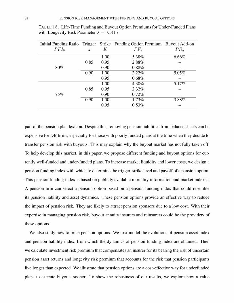
Tables 17 and 18 show the results for under-funded plans. In contrast to fully funded plans, a
higher λ reduces the triggering probability of pension options for under-funded plans, resulting in
lower funding option prices PFu. However, a higher λ increases buyout option premia PRu for
poorly funded plans. For instance, in Table 17, the price of the buyout add-on for a 75% funded plan
with z = 0.85 is PRu = 3.90% when λ = 0.0472. Table 18 shows that the buyout add-on premium
increases to 5.17% when λ goes up to 0.1415, even if the chance of triggering the option is lower in
this case. This result shows the opposing effects of λ on the buyout add-on and the funding option for
under-funded plans.

PENSION RISK MANAGEMENT WITH FUNDING AND BUYOUT OPTIONS 31
TABLE 15. Life-Time Funding and Buyout Option Premiums for Fully Funded Planswith Longevity Risk Parameter λ = 0.0472
Initial Funding Ratio Trigger Strike Funding Option Premium Buyout Add-onPFI0 z K PFw PRw
1.00 8.20% 2.80%0.80 0.95 6.54% –
100% 0.90 4.88% –1.00 6.36% 1.46%
0.70 0.90 4.49% –0.80 2.63% –
TABLE 16. Life-Time Funding and Buyout Option Premiums for Fully Funded Planswith Longevity Risk Parameter λ = 0.1415
Initial Funding Ratio Trigger Strike Funding Option Premium Buyout Add-onPFI0 z K PFw PRw
1.00 9.05% 4.29%0.80 0.95 7.22% –
100% 0.90 5.39% –1.00 7.30% 2.38%
0.70 0.90 5.17% –0.80 3.03% –
TABLE 17. Life-Time Funding and Buyout Option Premiums for Under-Funded Planswith Longevity Risk Parameter λ = 0.0472
Initial Funding Ratio Trigger Strike Funding Option Premium Buyout Add-onPFI0 z K PFu PRu
1.00 5.45% 4.99%0.85 0.95 2.91% –
80% 0.90 0.88% –0.90 1.00 2.31% 3.84%
0.95 0.71% –1.00 4.44% 3.90%
0.85 0.95 2.39% –75% 0.90 0.73% –
0.90 1.00 1.82% 2.94%0.95 0.56% –
7. CONCLUSION
Operating DB pensions has become a more and more difficult business for a firm. Unexpected
mandatory contributions to DB plans reduce resources available for business investments and ad-
versely affect a firm’s business performance. As a result, the phrase “pension buyout” has becomes
32 PENSION RISK MANAGEMENT WITH FUNDING AND BUYOUT OPTIONS
TABLE 18. Life-Time Funding and Buyout Option Premiums for Under-Funded Planswith Longevity Risk Parameter λ = 0.1415
Initial Funding Ratio Trigger Strike Funding Option Premium Buyout Add-onPFI0 z K PFu PRu
1.00 5.38% 6.66%0.85 0.95 2.88% –
80% 0.90 0.88% –0.90 1.00 2.22% 5.05%
0.95 0.68% –1.00 4.30% 5.17%
0.85 0.95 2.32% –75% 0.90 0.72% –
0.90 1.00 1.73% 3.88%0.95 0.53% –
part of the pension plan lexicon. Despite this, removing pension liabilities from balance sheets can be
expensive for DB firms, especially for those with poorly funded plans at the time when they decide to
transfer pension risk with buyouts. This may explain why the buyout market has not fully taken off.
To help develop this market, in this paper, we propose different funding and buyout options for cur-
rently well-funded and under-funded plans. To increase market liquidity and lower costs, we design a
pension funding index with which to determine the trigger, strike level and payoff of a pension option.
This pension funding index is based on publicly available mortality information and market indexes.
A pension firm can select a pension option based on a pension funding index that could resemble
its pension liability and asset dynamics. These pension options provide an effective way to reduce
the impact of pension risk. They are likely to attract pension sponsors due to a low cost. With their
expertise in managing pension risk, buyout annuity insurers and reinsurers could be the providers of
these options.
We also study how to price pension options. We first model the evolutions of pension asset index
and pension liability index, from which the dynamics of pension funding index are obtained. Then
we calculate investment risk premium that compensates an insurer for its bearing the risk of uncertain
pension asset returns and longevity risk premium that accounts for the risk that pension participants
live longer than expected. We illustrate that pension options are a cost-effective way for underfunded
plans to execute buyouts sooner. To show the robustness of our results, we explore how a value

PENSION RISK MANAGEMENT WITH FUNDING AND BUYOUT OPTIONS 33
change in a parameter affects pension option price. Our numerical examples show the reliability of
our pricing models with reasonable results.
REFERENCES
Bo, L., Y. Wang, and X. Yang (2010). Markov-modulated jump-diffusions for currency option pricing.
Insurance: Mathematics and Economics 46(3), 461 – 469.
Buckmann, C. (2014). De-risking your retiree pensions? Verizon court affirms plan sponsor rights to
shed obligations. http://www.pensionsbenefitslaw.com.
Bunkley, N. (2012). G.M. changes pensions for salaried workers. http://www.nytimes.com.
Cox, J. C., J. E. Ingersoll, and S. A. Ross (1985). A theory of the term structure of interest rates.
Econometrica 53(2), 385–407.
Cox, S. H. and Y. Lin (2007). Natural hedging of life and annuity mortality risks. North American
Actuarial Journal 11(3), 1–15.
Cox, S. H., Y. Lin, R. Tian, and J. Yu (2013). Managing capital market and longevity risks in a defined
benefit pension plan. Journal of Risk and Insurance 80(3), 585–619.
Cox, S. H., Y. Lin, R. Tian, and L. F. Zuluaga (2010). Portfolio risk management with CVaR-like
constraints. North American Actuarial Journal 14(1), 86–106.
Cox, S. H., Y. Lin, R. Tian, and L. F. Zuluaga (2013). Mortality portfolio risk management. Journal
of Risk and Insurance 80(4), 853–890.
Cox, S. H., Y. Lin, and S. Wang (2006). Multivariate exponential tilting and pricing implications for
mortality securitization. Journal of Risk and Insurance 73(4), 719–736.
Ebling, A. (2014). Companies prepare to dump pension plans in 2014. http://onforb.es/1fHDdNH.
Gerber, H. U. and E. S. Shiu (1994). Option pricing by Esscher transforms. Transactions of Society
of Actuaries 46, 99–191.
Gukaynak, R. S., B. Sack, and E. Swanson (2005). The sensitivity of long-term interest rates to
economic news: Evidence and implications for macroeconomic models. American Economic Re-
view 95(1), 425–436.
Hull, J. and A. White (1990). Pricing interest-rate-derivative securities. Review of Financial Stud-
ies 3(4), 573–592.
34 PENSION RISK MANAGEMENT WITH FUNDING AND BUYOUT OPTIONS
Lam, J. (2001). The cro is here to stay. Risk Management 48(4), 16–20.
LCP (2012). LCP pension buy-ins, buy-outs and longevity swaps 2012. http://www.lcp.uk.com.
Download on April 6, 2013.
Lee, R. D. and L. Carter (1992). Modelling and forecasting the time series of US mortality. Journal
of the American Statistical Association 87(419), 659–671.
Liebenberg, A. P. and R. E. Hoyt (2003). The determinants of enterprise risk management: Evidence
from the appointment of chief risk officers. Risk Management and Insurance Review 6(1), 37–52.
Lin, Y. and S. H. Cox (2005). Securitization of mortality risks in life annuities. Journal of Risk and
Insurance 72(2), 227–252.
Lin, Y. and S. H. Cox (2008). Securitization of catastrophe mortality risks. Insurance: Mathematics
and Economics 42(2), 628–637.
Lin, Y., S. Liu, and J. Yu (2013). Pricing mortality securities with correlated mortality indices. Journal
of Risk and Insurance 80(4), 921–948.
Lin, Y., R. D. MacMinn, and R. Tian (2015). De-risking defined benefit plans. Insurance: Mathemat-
ics and Economics 62. Forthcoming.
Lin, Y., R. D. MacMinn, R. Tian, and J. Yu (2015). Pension risk management in the enterprise risk
management framework. Working Paper, University of Nebraska, Illinois State University and
North Dakota State University.
Lin, Y., T. Shi, and A. Arik (2015). Pricing buy-ins and buy-outs. Working Paper, University of
Nebraska and Hacettepe University.
Lin, Y., K. S. Tan, R. Tian, and J. Yu (2014). Downside risk management of a defined benefit plan
considering longevity basis risk. North American Actuarial Journal 18(1), 68–86.
Longstaff, F. A. and E. S. Schwartz (1992). Interest rate volatility and the term structure: A two-factor
general equilibrium model. The Journal of Finance 47(4), 1259–1282.
Mathur, R. and S. Kaplan (2013). Reducing pension risk: The myths holding back plan sponsors.
http://pensionrisk.prudential.com.
Maurer, R., O. S. Mitchell, and R. Rogalla (2009). Managing contribution and capital market risk in
a funded public defined benefit plan: Impact of CVaR cost constraints. Insurance: Mathematics
and Economics 45(1), 25–34.

PENSION RISK MANAGEMENT WITH FUNDING AND BUYOUT OPTIONS 35
McDonald, R. L. (2013). Derivatives Markets (third ed.). Pearson.
Mercer LLC (2014, December). Mercer global pension buyout index.
http://www.mercer.com/newsroom/mercer-global-pension-buyout-index.html.
Merton, R. C. (1976). Option pricing when underlying stock returns are discontinuous. Journal of
Financial Economics 3(1-2), 125–144.
Milidonis, A., Y. Lin, and S. H. Cox (2011). Mortality regimes and pricing. North American Actuarial
Journal 15(2), 266–289.
Milliman (2015). Milliman analysis: January 2015 interest rates reach a record low of 3.38% with
abysmal effect on pension funding. http://us.milliman.com.
Nocco, B. W. and R. M. Stulz (2006). Enterprise risk management: Theory and practice. Journal of
Applied Corporate Finance 18(4), 8–20.
Wang, S. S. (1996). Premium calculation by transforming the layer premium density. ASTIN Bul-
letin 26(1), 71–92.
Wang, S. S. (2000). A class of distortion operations for pricing financial and insurance risks. Journal
of Risk and Insurance 67(1), 15–36.
Wang, S. S. (2001). A universal framework for pricing financial and insurance risks. In 6th AFIR
Proceedings, Number September, pp. 679–703. International Actuarial Association.
Wang, S. S. (2002). A universal framework for pricing financial and insurance risks. ASTIN Bul-
litin 32(2), 213–234.
Ward, M. (2014). 2014 annual buyout market watch report. http://www.jltgroup.com/content/UK.