perceptualdominantcolorextractionbymultidimensional...
TRANSCRIPT

Hindawi Publishing CorporationEURASIP Journal on Advances in Signal ProcessingVolume 2009, Article ID 451638, 13 pagesdoi:10.1155/2009/451638
Research Article
Perceptual Dominant Color Extraction by MultidimensionalParticle Swarm Optimization
Serkan Kiranyaz,1 Stefan Uhlmann (EURASIP Member),1 Turker Ince,2
and Moncef Gabbouj (EURASIP Member)1
1 Signal Processing Department, Tampere University of Technology, P.O. Box 553, 33101 Tampere, Finland2 Faculty of Computer Science, Izmir University of Economics, 35330 Izmir, Turkey
Correspondence should be addressed to Serkan Kiranyaz, [email protected]
Received 25 March 2009; Revised 20 September 2009; Accepted 7 December 2009
Recommended by Moon Kang
Color is the major source of information widely used in image analysis and content-based retrieval. Extracting dominant colorsthat are prominent in a visual scenery is of utmost importance since the human visual system primarily uses them for perceptionand similarity judgment. In this paper, we address dominant color extraction as a dynamic clustering problem and use techniquesbased on Particle Swarm Optimization (PSO) for finding optimal (number of) dominant colors in a given color space, distancemetric and a proper validity index function. The first technique, so-called Multidimensional (MD) PSO can seek both positionaland dimensional optima. Nevertheless, MD PSO is still susceptible to premature convergence due to lack of divergence. To addressthis problem we then apply Fractional Global Best Formation (FGBF) technique. In order to extract perceptually important colorsand to further improve the discrimination factor for a better clustering performance, an efficient color distance metric, which usesa fuzzy model for computing color (dis-) similarities over HSV (or HSL) color space is proposed. The comparative evaluationsagainst MPEG-7 dominant color descriptor show the superiority of the proposed technique.
Copyright © 2009 Serkan Kiranyaz et al. This is an open access article distributed under the Creative Commons AttributionLicense, which permits unrestricted use, distribution, and reproduction in any medium, provided the original work is properlycited.
1. Introduction
DOMINANT Color (DC) extraction is basically a dynamiccolor quantization process, which seeks for such prominentcolor centers that minimize the quantization error. Tothis end, studying human color perception and similaritymeasurement in the color domain becomes crucial and thereis a wealth of research performed in this field. For examplein [1], van den Broek et al. focused on the utilization ofcolor categorization (called as focal colors) for content-basedimage retrieval (CBIR) purposes and introduced a new colormatching method, which takes human cognitive capabilitiesinto account. They exploited the fact that humans tend tothink and perceive colors only in 11 basic categories. In[2], Mojsilovic et al. performed a series of psychophysicalexperiments analyzing how humans perceive and measuresimilarity in the domain of color patterns. One observationworth mentioning here is that the human eye cannot perceivea large number of colors at the same time, nor it is able to
distinguish similar (close) colors well. Based on this, theyshowed that at the coarsest level of judgment, the humanvisual system (HVS) primarily uses dominant colors (i.e., fewprominent colors in the scenery) to judge similarity.
The usual approach for DC extraction is to performclustering in a color domain. The most popular clusteringmethod, which is also used for MPEG-7 DC descriptor(DCD) [3], is K-means, [4]. However, clustering is amultimodal problem especially in high dimensions, whichcontains many suboptimum solutions resulting in over-and underclustering. Therefore, well-known deterministicmethods such as K-means, Max-Min [4], FCM [4], andSOM [4] are susceptible to get trapped to the closest localminimum since they are nothing but greedy descent meth-ods, which start from a random point in the solution spaceand perform a localized search. This fact eventually turnsthe focus on stochastic Evolutionary Algorithms (EAs) [5]such as Genetic Algorithms (GAs) [6], Genetic Programming(GP) [7], Evolution Strategies (ESs), [8] and Evolutionary
2 EURASIP Journal on Advances in Signal Processing
Programming (EP) [9], all of which are motivated by thenatural evolution process and thus make use of evolutionaryoperators. The common point of all is that EAs are inpopulation-based nature and can perform a global search.So they may avoid becoming trapped in a local optimumand find the optimum solution; however, this is neverguaranteed.
Conceptually speaking, Particle Swarm Optimization(PSO) [10–12], which has obvious ties with the EA family,lies somewhere in between GA and EP. Yet unlike GA, PSOhas no complicated evolutionary operators such as crossover,selection, and mutation. In a PSO process, a swarm ofparticles (or agents), each of which represents a potentialsolution to an optimization problem, navigate through thesearch space. Particles are initially distributed randomly overthe search space and the goal is to converge to the globaloptimum of a function or a system. Several researchers haveshown that PSO exhibits a better clustering performancethan the aforementioned techniques [12–15]; however, whenthe problem is multimodal, PSO may also become trapped inlocal optima [16] due to the premature convergence problemespecially when the search space is of high dimensions[12]. Furthermore, PSO has so far been applied to simpleclustering problems [12–15], where the data space is limitedand usually in low dimensions and the number of clusters(hence the solution space dimension) is kept reasonablylow (e.g., <10). Moreover, all clustering methods mentionedearlier are static in nature; that is, the number of clusters hasto be specified a priori. This is also true for PSO since in itsbasic form it can only be applied to a search space with afixed dimension. Particularly for dominant color extraction,the optimal (true) number of DCs in an image is unknownand should thus be determined within the (PSO) process.
In this paper, we shall address data clustering as anoptimization problem and present techniques, which extendPSO in a proper way to find optimal (number of) clustersin a multidimensional space. To alleviate the prematureconvergence problem, the so-called Fractional Global BestFormation (FGBF) collects all promising components fromeach particle and fractionally creates an artificial GlobalBest (GB) particle, the aGB, which may guide the swarmbetter than the swarm’s native gbest particle [11] in such away that the swarm can converge to the global optimum(or near-optimum) solution even in high dimensions andusually in earlier stages. In order to achieve a dynamicclustering where the optimum number of clusters is alsodetermined within the process, we shall then present the so-called MultiDimensional Particle Swarm Optimization (MDPSO) method, which extends the native structure of PSOparticles in such a way that they can make inter-dimensionalpasses with a dedicated dimensional PSO process [17].Therefore, in a multidimensional search space where theoptimum dimension is unknown, swarm particles can seekfor both positional and dimensional optima. In recent works,both techniques have been successfully applied over multi-dimensional nonlinear function minimization and 2D dataclustering [17], optimization over dynamic environments[18], and automatic design of artificial neural networks[19, 20], respectively. In this paper we adapt both techniques
to extract the optimal (number of) DCs in an image withrespect to a cluster validity index and color domain.
Cluster validity analysis is the assessment of the clusteringmethod’s output using a specific criterion for optimality, thatis, the so-called clustering validity index function [21]. Hencethe optimality of any clustering method can only be assessedwith respect to the validity index, which can be definedover a particular data representation with a proper distance(similarity) metric. Many existing DC extraction techniques,particularly the ones widely used in CBIR systems suchas MPEG-7 DCD, have severe drawbacks and thus show alimited performance. The main reason for this is becausemost of them are designed based on some heuristics ornaıve rules that are not formed with respect to what humansor more specifically the human visual system (HVS) finds“relevant” in color similarity. Therefore, it is of decisiveimportance that human color perception is considered whilstmodeling and describing any color composition of an image.In other words, when a particular color descriptor is designedentirely based on HVS and color perception rules, furtherdiscrimination power and hence certain improvements inretrieval performance can be achieved. For this reason weshall propose a fuzzy model to achieve a perceptual distancemetric over HSV (or HSL) color space, which provides meansof modeling color in a way HVS does. In this way thediscrimination between distinct colors is further enhanced,which in turns improves the clustering (and DC extraction)performance.
The rest of the paper is organized as follows. Section 2surveys related work on DC extraction whilst presenting abrief overview on data clustering. The applications of MDPSO and FGBF for optimal dynamic clustering and theproposed DC extraction technique are presented in detailin Section 3. Section 4 provides the experiments conductedover a real image database and discusses the results. Finally,Section 5 concludes the paper.
2. Related Work
There is a wealth of research done and still going onin developing efficient DC extraction methods, which canbe used in many applications, such as lossy compressiontechniques, mobile and hand-held devices, low-cost colordisplays, color look-up tables, and CBIR. In this article, weshall restrict the focus on the CBIR domain, which employscolor as the descriptor for image retrieval. We shall thenbriefly introduce major data clustering methods.
2.1. DC Descriptors. In order to solve the problems of staticquantization in color histograms, various DC descriptors,for example, [3, 22–25], have been developed using dynamicquantization with respect to image color content. DCs, ifextracted properly according to the aforementioned colorperception rules, can indeed represent the prominent colorsin any image. They have a global representation, which iscompact and accurate, and they are also computationallyefficient. MPEG-7 DC descriptor (DCD) is adopted as in[23] where the method is designed with respect to HVS

EURASIP Journal on Advances in Signal Processing 3
color perceptual rules. For instance, HVS is more sensitiveto changes in smooth regions than in detailed regions. Thuscolors are quantized more coarsely in the detailed regionswhile smooth regions have more importance. To exploit thisfact, a smoothness weight (w(p)) is assigned to each pixel(p) based on the variance in a local window. Afterwards,the General Lloyd Algorithm (GLA, also referred to as Linde-Buzo-Gray and it is equivalent to the well-known K-meansclustering method [4]) is used for color quantization. For acolor cluster Ci, its centroid ci is calculated by
ci =∑w(p)x(p)
∑w(p) , x
(p) ∈ Ci (1)
and the initial clusters for GLA are determined by using aweighted distortion measure, defined as,
Di =∑w(p)∥∥x(p)− ci
∥∥2, x
(p) ∈ Ci. (2)
This is used to determine which clusters to split until eithera maximum number of clusters (DCs), Nmax
DC , is achievedor a maximum allowed distortion criteria, εD, is met.Hence, pixels with smaller weights (detailed sections) areassigned fewer clusters so that the number of color clustersin the detailed regions where the likelihood of outliers’presence is high is therefore suppressed. As the final step,an agglomerative clustering (AC) is performed on the clustercentroids to further merge similar color clusters so that thereis only one cluster (DC) hosting all similar color componentsin the image. A similarity threshold TS is assigned to themaximum color distance possible between two similar colorsin a certain color domain (CIE-Luv, CIE-Lab, etc.). Anothermerging criterion is the color area; that is, any cluster shouldhave a minimum amount of coverage area, TA, so as to beassigned as a DC; otherwise, it will be merged with the closestcolor cluster since it is just an outlier. Another importantissue is the choice of the color space since a proper colorclustering scheme for DC extraction tightly relies on themetric. Therefore, a perceptually uniform color space shouldbe used and the most common ones are CIE-Luv and CIE-Lab, which are designed such that color distances perceivedby HVS are also equal in L2 (Euclidean) distance in thesespaces. For CIE-Luv, a typical value for TS is between 10 and25, TA is between 1% and 5%, and εD < 0.05 [3].
2.2. Data Clustering. As the process of identifying naturalgroupings in a multidimensional data space based on somedistance metric (e.g., Euclidean), data clustering can bedivided into two main categories: hierarchical and partitional[4]. Each category then has a wealth of subcategories anddifferent algorithmic approaches for finding the clusters.Clustering can also be performed in two different modes:hard (or crisp) and fuzzy. K-means [4] is a well knownand widely used hard clustering method, which first assignseach data point to one of the K cluster centroids and thenupdates them to the mean of their associated points. Yet asa hard clustering method, K-means suffers from the severaldrawbacks, for example, (1) The number of clusters, K, needsto be set in advance, (2) Its performance directly depends
on the initial (random) centroid positions as the methodconverges to the closest local optima and (3) K-means is alsodependent on the data distribution. There are many otherclustering variants that are skipped where an extensive surveycan be found in [4, 26].
A hard clustering technique based on the basic PSO(bPSO) was first introduced by Omran et al. in [13] and thiswork showed that the bPSO can outperform K-means, FCM,KHM, and some other state-of-the-art clustering methodsin any (evaluation) criteria. This is indeed an expectedoutcome due to the PSO’s aforementioned ability to copewith the local optima by maintaining a guided randomsearch operation through the swarm particles. In clustering,similar to other PSO applications, each particle represents apotential solution at a particular time t, that is, the particle ain the swarm, ξ = {x1, . . . , xa, . . . , xS}, is formed as xa(t) ={ca,1, . . . , ca, j , . . . , ca,K} ⇒ xa, j(t) = ca, j where ca, j is the jth(potential) cluster centroid in N dimensional data space andK is the number of clusters fixed in advance. Note that thedata space dimension, N, is now different than the solutionspace dimension, K. Furthermore, the fitness (validity index)function, f that is to be optimized, is formed with respect totwo widely used criteria in clustering:
(i) Compactness: Data items in one cluster should besimilar or close to each other in N dimensionalspace and different or far away from the others whenbelonging to different clusters.
(ii) Separation: Clusters and their respective centroidsshould be distinct and well-separated from eachother.
The fitness functions for clustering are then formedas a regularization function fusing both Compactness andSeparation criteria and in this problem domain they areknown as clustering validity indices. The minimization of avalidity index will simultaneously try to minimize the intra-cluster distances (for better Compactness) and maximizethe inter-cluster distance (for better Separation). In such aregularization approach, different priorities (weights) canbe assigned to both subobjectives via proper setting ofweight coefficients; however, this makes the approach strictlyparameter dependent. Another traditional and well-knownvalidity index is Dunn’s index [27], which suffers from twodrawbacks. It is computationally expensive and sensitive tonoise [21]. Several variants of Dunn’s index were proposedin [26] where robustness against noise is improved. Thereare many other validity indices, that is, proposed by Turi[28], Davies and Bouldin [29], Halkidi et al. [21], and soforth. A throughout survey can be found in [21]. Most ofthem presented promising results; however, none of themcan guarantee the “optimum” number of clusters in everyclustering scheme.
Although PSO-based clustering outperforms many well-known clustering methods, it still suffers from two majordrawbacks. The number of clusters K (being the solutionspace dimension as well) must still be specified in advanceand similar to other bPSO applications, the method tends totrap in local optima particularly when the complexity of the

4 EURASIP Journal on Advances in Signal Processing
clustering scheme increases. This also involves the dimensionof the solution space, that is, convergence to “optimum”number of “true” clusters can only be guaranteed for lowdimensions. This is also true for dynamic clustering schemes,DCPSO [15] and MEPSO [22], both of which eventuallypresent results only in low dimensions and for simpledata distributions. All these drawbacks and limitations havesuccessfully been addressed in [17].
3. The Proposed DC Extraction Technique
Humans tend to think and describe color the way they per-ceive it. Therefore, in order to achieve a color (dis) similaritymetric taking HVS into account, HSV (or HSL), which is aperceptual color space and provides means of modeling colorin a way HVS does, is used in the proposed technique forextracting dominant colors. Note that in a typical image with24-bit RGB representation, there can be several thousands ofdistinct colors, most of which cannot be perceived by HVS.Therefore, to reduce the computational complexity of RGBto HSV color transformation and particularly to speed upthe dynamic clustering process via MD PSO and FGBF, a pre-processing step, which creates a limited color palette in RGBcolor domain, is first performed. In this way such a massive,yet unperceivable amount of colors in RGB domain can bereduced to a reasonable number, for example, 256 < n < 512.To this end, we used the Median Cut method [30] becauseit is fast (i.e., O(n)) and for such a value of n, it yields animage which can hardly be (colorwise) distinguished fromthe original. Only the RGB color components in the colorpalette are then transformed into HSV (or HSL) color spaceover which the proposed dynamic clustering technique isapplied to extract the dominant colors, as explained next.
3.1. Dynamic Clustering by MD PSO with FGBF. Based onthe earlier discussion it is obvious that the clustering problemrequires the determination of the solution space dimension(i.e., number of clusters, K) and an effective mechanismto avoid local optima (i.e., traps, both dimensionally andspatially) particularly in complex clustering schemes in highdimensions (e.g., K > 10). The former requirement justifiesthe use of the proposed MD PSO technique while the lattercalls for FGBF. A brief description of both techniques is givenin the appendix and see [17] for details.
At time t, a particle a in the swarm, ξ = {x1, . . . ,xa, . . . , xS}, has the positional component formed as,
xxxda(t)a (t) = {ca,1, . . . , ca, j , . . . , ca,xda(t)} ⇒ xxxda(t)
a, j (t) = ca, j
meaning that it represents a potential solution (i.e., acluster centroid) for the xda(t) number of clusters whilst jthcomponent being the jth cluster centroid. Apart from theregular limits such as (spatial) velocity, Vmax, dimensionalvelocity, VDmax, and dimension range Dmin ≤ xda(t) ≤Dmax, the (variable) N dimensional data space is also limited
with some practical spatial range, that is, Xmin < xxxda(t)a (t) <
Xmax. In case this range is exceeded even for a single
dimension j, xxxda(t)a, j (t), then all positional components of
the particle for the respective dimension xda(t) are initializedrandomly within the range and this further contributes to
the overall diversity. Let Z be the set of points, Z = {zp}, inthe N-dimensional data space. The following validity indexis used to obtain computational simplicity with minimal orno parameter dependency,
f(xxxda(t)
a ,Z)= Qe
(xxxda(t)
a
)(xda(t))α, where
Qe
(xxxda(t)
a
)= 1xda(t)
xda(t)∑
j=1
∑∀zp∈xxxda(t)
a, j
∥∥∥xxxda(t)
a, j − zp∥∥∥
∥∥∥xxxda(t)
a
∥∥∥
,
(3)
where Qe is the quantization error (or the average intra-cluster distance) as the Compactness term and (xda(t))α is theSeparation term, by simply penalizing higher cluster numberswith an exponential, α > 0. Using α = 1, the validity indexyields the simplest form and becomes entirely parameter-free.
On the other hand, (hard) clustering has some con-
straints. Let Cj={xxxda(t)a, j (t)}={ca, j}, for all j ∈ [1, xda(t)],
be the set of data points assigned to a (potential) cluster
centroid xxxda(t)a, j (t) for a particle a at time t. The partitions
Cj , for all j ∈ [1, xda(t)] should maintain the followingconstraints:
(1) Each data point should be assigned to one cluster set:⋃xda(t)
j=1 Cj = Z.
(2) Each cluster should contain at least one data point:Cj /={φ}, for all j ∈ [1, xda(t)].
(3) Two clusters should have no common data points:Ci ∩ Cj = {φ}, i /= j and for all i, j ∈ [1, xda(t)].
In order to satisfy the 1st and 3rd (hard) clustering con-straints, before computing the clustering fitness score viathe validity index function in (3), all data points are firstassigned to the closest centroid. Yet there is no guarantee for
the fulfillment of the 2nd constraint since xxxda(t)a (t) is set
(updated) by the internal dynamics of the MD PSO processand hence any dimensional component (i.e., a potential
cluster candidate), xxxda(t)a, j (t), can be in an abundant position
(i.e., no closest data point exists). To avoid this, a highpenalty is set for the fitness score of the particle, that is,
f (xxxda(t)a ,Z) ≈ ∞, if {xxxda(t)
a, j } = {φ} for any j.The major outlines so far given are sufficient for applying
the MD PSO technique to dynamic clustering and for thispurpose the details for the application of FGBF over MD PSOcan be found in [17].
3.2. Fuzzy Model over HSV-HSL Color Domains. Let c1 ={h1, s1, v1} and c2 = {h2, s2, v2} be two colors in HSVdomain. Assume for the sake of simplicity that the hueis between 0 to 360 degrees and both s and v are unitnormalized. The normalized Euclidean distance between sand v can be defined as follows:
‖c1 − c2‖2 = (v1 − v2)2 + (s1 cos(h1)− s2 cos(h2))2
+ (s1 sin(h1)− s2 sin(h2))2.(4)

EURASIP Journal on Advances in Signal Processing 5
During the dynamic clustering process by MD PSO andFGBF, the problem of using this equation for comput-ing a color distance between a candidate color centroid,xxda, j(t), for all j ∈ [1,d] and a color in the palette, zp ∈xxda(t), as in (3) is that it has a limited discriminationpower between distinct colors, as it basically yields arbitraryfractional numbers despite the fact that HVS finds “nosimilarity” in between. Therefore, instead of using thistypical distance metric for all color pairs, we adopt aperceptual approach in order to improve discriminationbetween different colors. Recall from the earlier discussionthat humans can recognize and distinguish 8 to 12 colors.Recall that in [1], the authors exploited the fact that humanstend to think and perceive colors only in 11 basic categories.Hence above a certain hue difference between two colors,it is obvious that they become entirely different for HVS;for example, yellow and green are as different as yellowand blue or cyan or black or purple, and so forth. So ifthe hue difference is above a certain limit, a maximumdifference should be used (i.e., 1.0). We have selected anupper limit by considering distinct colors number as only8, therefore, the perceptual threshold is ΔTH = 360/8 =45 degrees. In practice, however, even a lower hue thresholdcan also be used, because two colors, for instance, with 40degrees of hue difference can hardly have any similarity—yet 45 degrees present a safe margin leaving any subjectivityout.
We then use a fuzzy color model for further discrimina-tion. As shown in Figure 1, for a fixed hue, for example, redfor HSV and green for HSL, a typical saturation (S) versusValue (V) or Lightness (L) plot can be partitioned into 5regions: White (W), Black (B), Gray (G), Color (C), andFuzzy (F), which is a transition area among others. W , Band G are the areas where there is absolutely no color (hue)component whereas in F there is a hint of a color presencewith a known hue but perhaps not fully saturated. In C, thecolor described by its hue is fully perceivable with a varyingsaturation and value. It is a fact that the borders among colorregions are highly subjective and this is the sole reason to usea large Fuzzy region, so as to address this subjectivity in colorperception and thus to contain the error. This is the reasonwhy there is no need for drawing precise boundaries of F(even if possible) or the boundaries between W ↔ G andB ↔ G because between two colors, say one in C and onein F, or both in C or both in F, the same distance metricshall anyway be applied (as in (4)) provided that they havehue differences less than ΔTH thus presenting some degree ofcolor similarity. This is not a condition in other cases whereat least one color is from either of the “no color” areas. Forinstance, between W ↔ G and B ↔ G, the distance shouldonly be computed over V (or L) components because theyhave no perceivable color components. The boundaries areonly important to distinguish areas such as C, W and B(and between C ↔ G) where there is no similarity amongthem. Therefore, as shown in the HSL map on the rightwith blue arrows, if two colors, despite the fact that theyhave similar hues (i.e., ΔH < ΔTH), happen to be in suchregions, maximum distance (1.0) shall be applied rather thancomputing (4).
HSV1
V
0 S 1
(a)
HSL1
L
0 S 1
(b)
W
G
F
C
B
(c)
W
G F C
B
(d)
Figure 1: Fuzzy model for distance computation in HSV and HSLcolor domains (best viewed in color).
4. Experimental Results
We have made comparative evaluations against MPEG-7 DCD over a sample database with 110 images, whichare selected from Corel database in such a way that theirprominent colors (DCs) are easy to be recognized by ground-truth. We used the typical internal PSO parameters (c1, c2,and w) as in [31]. Unless otherwise stated, in all experimentsin this section, the two critical PSO parameters, swarm size(S), and number of iterations (iterNo) are set as 100 and 500,respectively. Their effects over the DC extraction are thenexamined. The dimension (search) range for DC extractionis set as Dmin = 2, Dmax = 25. This setting is in harmonywith the maximum number of DCs set by the MPEG-7DCD, that is, Nmax
DC = 25. Finally the size of the initialcolor palette created by the Median Cut method is set as256.
4.1. Comparative Evaluations against MPEG-7 DCD. Inorder to demonstrate the strict parameter dependency ofMPEG-7 DCD, we have varied only two parameters, TA andTS whilst keeping the others fixed, that is, Nmax
DC = 25, andεD = 0.01. Experiments are performed with three sets ofparameters: P1: TA = 1%, TS = 15, P2: TA = 1%, TS = 25and P3: TA = 5%, TS = 25. The number of DCs (perimage) plots obtained from the 110 images in the sampledatabase using each parameter set can be seen in Figure 2. Itis evident from the figure that the number of DCs is strictlydependent on the parameters used and can vary significantly,for example, between 2 to 25.

6 EURASIP Journal on Advances in Signal Processing
0
5
10
15
20
25
DC
nu
mbe
r
0 20 40 60 80 100 120
Image number
Ts = 15, Ta = 1%
Ts = 25, Ta = 1%Ts = 25, Ta = 5%
Figure 2: Number of DC plot from three MPEG-7 DCDs withdifferent parameter set over the sample database.
Figures 3 and 4 show some visual examples from thesample database. In both figures, the first column shows theoutput of the Median-Cut algorithm with 256 (maximum)colors, which is almost identical to the original image. Thesecond and the rest of the three columns show the back-projected images using the DCs extracted from the proposedtechnique and MPEG-7 DCD with those three parametersets, respectively. Note that the parts, where DC centroidscannot be accurately localized or missed completely byMPEG-7 DCD, are pointed with (yellow) arrows. There isan ambiguity for deciding which parameter set yields thebest visual performance although it would have naturallybeen expected from the first set, P1: TA = 1%, TS = 15,where the highest number of DCs is extracted (see the redplot in Figure 2), but it is evident that P2 and P3 can alsoyield “comparable or better” results; however it is a highlysubjective matter.
According to the results, one straightforward conclusionis that not only does the number of DCs significantly varybut DC centroids, as well, change drastically depending onthe parameter values used. On the other hand, it is obviousthat the best DC extraction performance is achieved by theproposed technique, where none of the prominent colorsare missed or mislocated whilst the “true” number of DCsis extracted. However, we do not and, in any way, cannotclaim that the proposed technique achieves the minimumquantization error (or the mean square error, MSE), dueto two reasons. First, the optimization technique is appliedover a regularization (fitness) function where the quanti-zation error minimization (i.e., minimum Compactness) isonly one part of it. The other part, implying maximumSeparation, presents a constraint so that minimum MSE hasto be achieved using the least number of clusters (DCs).The second and the main reason is that computation ofMSE is typically performed in RGB color space, using theEuclidean metric. Recall that the proposed DC extractionis performed over HSV (or HSL) color domain, which isdiscontinuous and requires nonlinear transformations, andusing a fuzzy distance metric with respect to the HVSperceptual rules for enhancing the discrimination power.Therefore, the optimization in this domain using such a fuzzy
metric obviously cannot ensure a minimum MSE in RGBdomain. Besides that, several studies show that MSE is notan appropriate metric for visual (or perceptual) quality (e.g.,[32]) and thus we hereby avoid using it as a performancemeasure.
4.2. Robustness and Parameter Invariance of the ProposedMethod. Due to its stochastic nature, there is a concernabout robustness (or repeatability) of the results. In thissection, we perform several experiments to examine whetheror not the results are consistent in regard to accuracy ofthe DC centroids and their numbers. Repeatability wouldbe a critical problem for deterministic methods such as K-means, and Min-Max. if the initial color (cluster) centroidsare randomly chosen, as the original algorithm suggests.Eventually such methods would create different clusteringscheme each time they are performed since they are boundto get trapped to the nearest local optimum from the initialposition. The solution to this problem induced by MPEG-7 DCD method is to change the random initialization partto a fixed (deterministic) initial assignment to the existingdata points so that the outcome, DC centroids and thenumber of DCs extracted, will be the same each time thealgorithm is performed over a particular image with the sameparameters. This would also be a practical option for theproposed technique, that is, fixing the initialization stage andusing a constant seed for the random number generator thatMD PSO uses. However, as a global optimization method,we shall demonstrate that MD PSO with FGBF can most ofthe time converge to (near-) optimal solutions, meaning that,the number of DCs and their centroids extracted from theproposed dynamic clustering technique shall be consistentand perceptually intact. Furthermore, in order to show thatsignificant variations for two major parameters, iterNo andS, do not cause drastic changes on the DC extraction, wewill use three parameter sets: P1: S = 50, iterNo = 500,P2: S = 50, iterNo = 1000, and P3: S = 100, iterNo= 1000. With each parameter set, we run the proposedtechnique (with random initialization and random seeds)100 times over two images. The DC number histograms perimage and per parameter set are as shown in Figure 5. Inthe first image (left), it is certain that the number of DCsis either 2 or 3, as one might argue that the yellowish colorof the dot texture over the object can be counted as a DCor not. For the image on the right, it is rather difficult todecide the exact number of DCs, since apart from blue, theremaining 5 colors, red, pink, yellow, green, and brown havecertain shades. It is, first of all, obvious that the proposedtechnique is parameter invariant since in both cases, thesignificant parameter variations, (particularly from P1 to P3where both iterNo and S are doubled) only make a slightdifference over the histograms. A high degree of robustness(repeatability) is also achieved since all runs in the firstimage yielded either 2 or 3 DCs, as desired, and >95% ofthe runs in the second image; the number of DCs is inthe range 16 ± 1. Among the back-projected images, it isevident that quite similar/almost identical DCs are anywayextracted even though they have different number of DCs

EURASIP Journal on Advances in Signal Processing 7
Median-cut(original) Proposed
MPEG-7DCD (P1)
MPEG-7DCD (P2)
MPEG-7DCD (P3)
(a)
(b)
(c)
(d)
(e)
Figure 3: The DC extraction results over 5 images from the sample database (best viewed in color).
(e.g., see the two with 14 and 18 DCs). As a result of theperceptual model used, the number of DCs can slightly vary,somewhat reflecting the subjectivity in HVS color perception,but similar DCs are extracted by the proposed techniqueregardless of the parameter set used.
4.3. Computational Complexity Analysis. The computationalcomplexity of the proposed method depends on two distinctprocesses. First is the preprocessing stage which creates alimited color palette in RGB color domain using Median Cutmethod and the following RGB to HSV color transformation.Recall that Median Cut method is a fast method (i.e., O(n)),which has the same computational complexity as K-means.The following color transformation has an insignificantprocessing time since it is only applied to a reduced numberof colors. The computational complexity analysis for thedynamic clustering technique based on MD-PSO with FGBFis performed in [17]. Moreover, the complexity of the validityindex used has a direct impact over the total computational
cost since for each particle (and at each iteration) it is usedto compute the fitness of that particle. This is the mainreason of using such a simple (and parameter independent)validity index as in (3). In that, the proposed fuzzy colormodel makes the computational cost primarily dependanton the color structure of the image because the normalizedEuclidean distance that is given in (4) and is used withinthe validity index function is obviously quite costly; however,recall that it may not be used at all for such color pairs thatdo not show any perceptual color similarity. This furthercontributes the infeasibility of performing an accurate com-putational complexity analysis for the proposed technique.For instance, using a PC with P-IV 3 GHz CPU and 1 GBRAM, the proposed DC extraction technique with parameterset P1 took 126 and 911 milliseconds, respectively, for thetwo sample images shown in Figure 5. In short, as any otherevolutionary algorithm the DC extraction based on MD PSOwith FGBF is slow in nature and may require indefiniteamount of iterations to converge to the global solution.
8 EURASIP Journal on Advances in Signal Processing
Median-cut(original)
Proposed MPEG-7DCD (P1)
MPEG-7DCD (P2)
MPEG-7DCD (P3)
(a)
(b)
(c)
(d)
(e)
Figure 4: The DC extraction results over 5 images from the sample database (best viewed in color).
5. Conclusions
In this paper, we first presented two efficient techniques, MDPSO and FGBF, as a solution to common drawbacks of thefamily of PSO methods such as a priori knowledge of thesearch space dimension and premature convergence to localoptima. A novel dynamic clustering technique based on MDPSO with FGBF is then proposed and applied for extracting“true” number of dominant colors in an image. In order to
improve the discrimination among different colors, a fuzzymodel over HSV (or HSL) color space is then proposed so asto achieve such a distance metric that reflects HVS perceptionof color (dis) similarity.
The DC extraction experiments using MPEG-7 DCDhave shown that the method, although a part of the MPEG-7standard, is highly dependent on the parameters. Moreover,since it is entirely based on K-means clustering method, itcan create artificial colors and/or misses some important
EURASIP Journal on Advances in Signal Processing 9
Image 1
(a)
Image 2
(b)
0
20
40
60
80
100
P1
0 5 10 15 20 25 30
(c)
0
10
20
30
40
50
60
70
P1
0 5 10 15 20 25 30
(d)
0
20
40
60
80
100
P2
0 5 10 15 20 25 30
(e)
0
10
20
30
40
50
60
70
P2
0 5 10 15 20 25 30
(f)
0
20
40
60
80
100
P3
0 5 10 15 20 25 30
(g)
0
10
20
30
40
50
60
P3
0 5 10 15 20 25 30
(h)
Figure 5: DC number histograms of 2 sample images using 3 parameter sets. Some typical back-projected images with their DC numberpointed are shown within the histogram plots (best viewed in color).
10 EURASIP Journal on Advances in Signal Processing
DCs due to its convergence to local optima, thus yieldingcritical over- and under-clustering. Consequently, a mixtureof different colors, and hence artificial DCs or DCs withshifted centroids, may eventually occur. This may also causesevere degradations over color textures since the regulartextural pattern cannot be preserved if the true DC centroidsare missed or shifted. Using a simple clustering validityindex, we have successfully addressed these problems and asuperior DC extraction is achieved with ground-truth DCs.The optimum number of DCs can slightly vary on someimages, but the number of DCs on such images is hardlydefinitive, rather subjective and thus on such occasionsthe dynamic clustering based on a stochastic optimizationtechnique can converge to some near-optimal solutions. Theproposed technique shows a high level of robustness forparameter invariance and hence the main idea is that insteadof struggling to fine tune several parameters to improveperformance, which is not straightforward, if possible at all,the focus can now be drawn to designing better validity indexfunctions or improving the ones for the purpose of higherDC extraction performance in terms of perceptual quality,which shall be the subject to our future work.
Appendices
A. MD PSO Algorithm
Instead of operating at a fixed dimension N, the MDPSO algorithm is designed to seek both positional anddimensional optima within a dimension range (Dmin ≤N ≤ Dmax). In order to accomplish this, each particle hastwo sets of components, each of which has been subjectedto two independent and consecutive processes. The firstone is a regular positional PSO, that is, the traditionalvelocity updates and following positional moves in N-dimensional search (solution) space. The second one isa dimensional PSO, which allows the particle to navigatethrough dimensions. Accordingly, each particle keeps trackof its last position, velocity and personal best position(pbest) in a particular dimension so that when it revisits thesame dimension at a later time, it can perform its regular“positional” fly using this information. The dimensionalPSO process of each particle may then move the particleto another dimension where it will remember its positionalstatus and keep “flying” within the positional PSO processin this dimension, and so on. The swarm, on the otherhand, keeps track of the gbest particles in all dimensions,each of which, respectively, indicates that the best (global)position so far achieved and can thus be used in the regularvelocity update equation for that dimension. Similarly thedimensional PSO process of each particle uses its personalbest dimension in which the personal best fitness score hasso far been achieved. Finally, the swarm keeps track of theglobal best dimension, dbest, among all the personal bestdimensions. The gbest particle in dbest dimension representsthe optimum solution (and the optimum dimension).
For the description of the positional and dimensionalcomponents, we shall use the following two-letter notation
rule for parameterization: the first letter signifies whether itis a position (x) or velocity (v) component and the secondletter corresponds to the type of the component: positional(x) or dimensional (d). As in PSO notation, we also used y forpersonal best (pbest) position for the positional component.Therefore, the following enlists all the components of MDPSO:
(i) xxxda(t)a, j (t): jth component (dimension) of the posi-
tion of particle a, in dimension xda(t),
(ii) vxxda(t)a, j (t): jth component (dimension) of the velocity
of particle a, in dimension xda(t),
(iii) xyxda(t)a, j (t): jth component (dimension) of the per-
sonal best (pbest) position of particle a, in dimensionxda(t),
(iv) xydj (t): jth component (dimension) of the global bestposition of swarm, in dimension d,
(v) xda(t): dimension component of particle a,
(vi) vda(t): velocity component of dimension of particlea,
(vii) xda(t): personal best dimension component of parti-cle a,
(viii) gbest(d): global best particle index in dimension d.
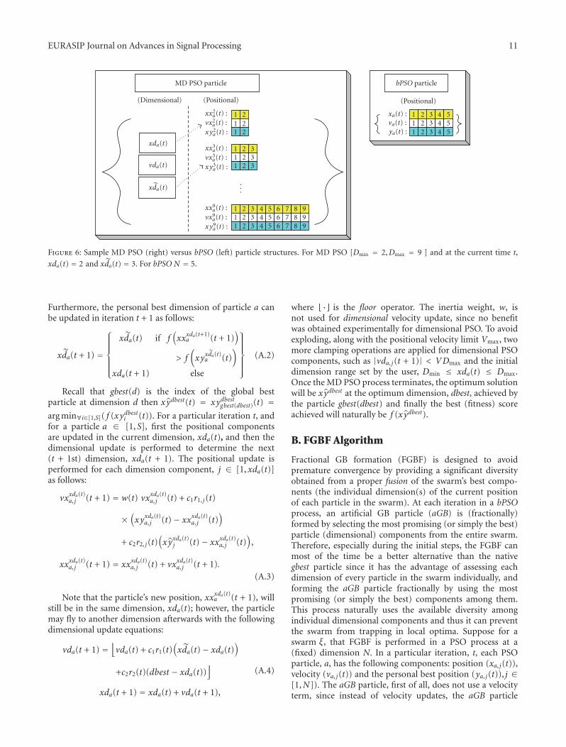
Figure 6 shows sample MD PSO and bPSO particles withindex a. The bPSO particle that is at a (fixed) dimension,N = 5, contains only positional components whereasMD PSO particle contains both positional and dimensionalcomponents, respectively. In the figure the dimension rangefor the MD PSO is given between 2 and 9; therefore theparticle contains 8 sets of positional components (one foreach dimension). In this example, the current dimensionwhere the particle a resides is 2 (xda(t) = 2) whereas its
personal best dimension is 3 (xda(t) = 3). Therefore, attime t, a positional PSO update is first performed over thepositional elements, xx2
a(t), and then the particle may moveto another dimension by the dimensional PSO.
Let f denote the dimensional fitness function that is tobe optimized within a certain dimension range (Dmin ≤ N ≤Dmax). Without loss of generality assume that the objectiveis to find the minimum (position) of f at the optimumdimension within a multidimensional search space. Assumethat the particle a visits (back) the same dimension after Titerations (i.e., xda(t) = xda(t + T)), then the personal bestposition can be updated in iteration t + T as follows,
xyxda(t+T)a, j (t + T)
=
⎧⎪⎪⎪⎪⎨
⎪⎪⎪⎪⎩
xyxda(t)a, j (t) if f
(xxxda(t+T)
a (t + T))
> f(xyxda(t)
a (t))
xxxda(t+T)a, j (t + T) else
⎫⎪⎪⎪⎪⎬
⎪⎪⎪⎪⎭
∀ j ∈ [1, xda(t)].
(A.1)
EURASIP Journal on Advances in Signal Processing 11
MD PSO particle
(Dimensional)
xda(t)
vda(t)
xda(t)
(Positional)
xx2a(t) :
vx2a(t) :
xy2a(t) :
111
222
xx3a(t) :
vx3a(t) :
xy3a(t) :
111
222
333
...
xx9a(t) :
vx9a(t) :
xy9a(t) :
111
222
333
444
555
666
777
888
999
bPSO particle
(Positional)
xa(t) :va(t) :ya(t) :
111
222
333
444
555
Figure 6: Sample MD PSO (right) versus bPSO (left) particle structures. For MD PSO [Dmin = 2,Dmax = 9 ] and at the current time t,
xda(t) = 2 and xda(t) = 3. For bPSO N = 5.
Furthermore, the personal best dimension of particle a canbe updated in iteration t + 1 as follows:
xda(t + 1) =
⎧⎪⎪⎪⎪⎨
⎪⎪⎪⎪⎩
xda(t) if f(xxxda(t+1)
a (t + 1))
> f(
xyxda(t)a (t)
)
xda(t + 1) else
⎫⎪⎪⎪⎪⎬
⎪⎪⎪⎪⎭
(A.2)
Recall that gbest(d) is the index of the global bestparticle at dimension d then xydbest(t) = xydbestgbest(dbest)(t) =arg min∀i∈[1,S]( f (xydbesti (t)). For a particular iteration t, andfor a particle a ∈ [1, S], first the positional componentsare updated in the current dimension, xda(t), and then thedimensional update is performed to determine the next(t + 1st) dimension, xda(t + 1). The positional update isperformed for each dimension component, j ∈ [1, xda(t)]as follows:
vxxda(t)a, j (t + 1) = w(t) vxxda(t)
a, j (t) + c1r1, j(t)
×(xyxda(t)
a, j (t)− xxxda(t)a, j (t)
)
+ c2r2, j(t)(xyxda(t)
j (t)− xxxda(t)a, j (t)
),
xxxda(t)a, j (t + 1) = xxxda(t)
a, j (t) + vxxda(t)a, j (t + 1).
(A.3)
Note that the particle’s new position, xxxda(t)a (t + 1), will
still be in the same dimension, xda(t); however, the particlemay fly to another dimension afterwards with the followingdimensional update equations:
vda(t + 1) =⌊vda(t) + c1r1(t)
(xda(t)− xda(t)
)
+c2r2(t)(dbest − xda(t))⌋
xda(t + 1) = xda(t) + vda(t + 1),
(A.4)
where �·� is the floor operator. The inertia weight, w, isnot used for dimensional velocity update, since no benefitwas obtained experimentally for dimensional PSO. To avoidexploding, along with the positional velocity limit Vmax, twomore clamping operations are applied for dimensional PSOcomponents, such as |vda, j(t + 1)| < VDmax and the initialdimension range set by the user, Dmin ≤ xda(t) ≤ Dmax.Once the MD PSO process terminates, the optimum solutionwill be xydbest at the optimum dimension, dbest, achieved bythe particle gbest(dbest) and finally the best (fitness) scoreachieved will naturally be f (xydbest).
B. FGBF Algorithm
Fractional GB formation (FGBF) is designed to avoidpremature convergence by providing a significant diversityobtained from a proper fusion of the swarm’s best compo-nents (the individual dimension(s) of the current positionof each particle in the swarm). At each iteration in a bPSOprocess, an artificial GB particle (aGB) is (fractionally)formed by selecting the most promising (or simply the best)particle (dimensional) components from the entire swarm.Therefore, especially during the initial steps, the FGBF canmost of the time be a better alternative than the nativegbest particle since it has the advantage of assessing eachdimension of every particle in the swarm individually, andforming the aGB particle fractionally by using the mostpromising (or simply the best) components among them.This process naturally uses the available diversity amongindividual dimensional components and thus it can preventthe swarm from trapping in local optima. Suppose for aswarm ξ, that FGBF is performed in a PSO process at a(fixed) dimension N. In a particular iteration, t, each PSOparticle, a, has the following components: position (xa, j(t)),velocity (va, j(t)) and the personal best position (ya, j(t)), j ∈[1,N]). The aGB particle, first of all, does not use a velocityterm, since instead of velocity updates, the aGB particle
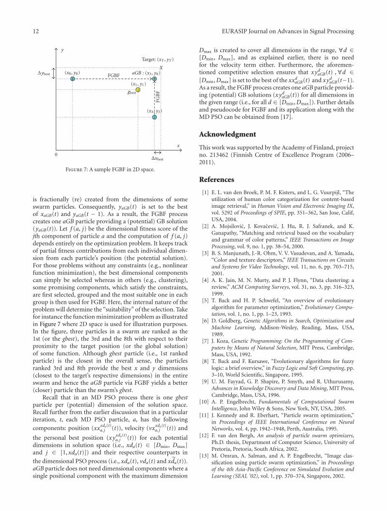
12 EURASIP Journal on Advances in Signal Processing
y
x
Δybest (x8, y8)FGBF
Target: (xT , yT )
XaGB : (x3, y8)
+(x1, y1)
gbest
(x3, y3)
FGB
FΔxbest
0
8
3
1
Figure 7: A sample FGBF in 2D space.
is fractionally (re) created from the dimensions of someswarm particles. Consequently, yaGB(t) is set to the bestof xaGB(t) and yaGB(t − 1). As a result, the FGBF processcreates one aGB particle providing a (potential) GB solution(yaGB(t)). Let f (a, j) be the dimensional fitness score of thejth component of particle a and the computation of f (a, j)depends entirely on the optimization problem. It keeps trackof partial fitness contributions from each individual dimen-sion from each particle’s position (the potential solution).For those problems without any constraints (e.g., nonlinearfunction minimization), the best dimensional componentscan simply be selected whereas in others (e.g., clustering),some promising components, which satisfy the constraints,are first selected, grouped and the most suitable one in eachgroup is then used for FGBF. Here, the internal nature of theproblem will determine the “suitability” of the selection. Takefor instance the function minimization problem as illustratedin Figure 7 where 2D space is used for illustration purposes.In the figure, three particles in a swarm are ranked as the1st (or the gbest), the 3rd and the 8th with respect to theirproximity to the target position (or the global solution)of some function. Although gbest particle (i.e., 1st rankedparticle) is the closest in the overall sense, the particlesranked 3rd and 8th provide the best x and y dimensions(closest to the target’s respective dimensions) in the entireswarm and hence the aGB particle via FGBF yields a better(closer) particle than the swarm’s gbest.
Recall that in an MD PSO process there is one gbestparticle per (potential) dimension of the solution space.Recall further from the earlier discussion that in a particulariteration, t, each MD PSO particle, a, has the following
components: position (xxxda(t)a, j (t)), velocity (vxxda(t)
a, j (t)) and
the personal best position (xyxda(t)a, j (t)) for each potential
dimensions in solution space (i.e., xda(t) ∈ [Dmin, Dmax]and j ∈ [1, xda(t)]) and their respective counterparts in
the dimensional PSO process (i.e., xda(t), vda(t) and xda(t)).aGB particle does not need dimensional components where asingle positional component with the maximum dimension
Dmax is created to cover all dimensions in the range, ∀d ∈[Dmin, Dmax], and as explained earlier, there is no needfor the velocity term either. Furthermore, the aforemen-tioned competitive selection ensures that xydaGB(t) ,∀d ∈[Dmin,Dmax] is set to the best of the xxdaGB(t) and xydaGB(t−1).As a result, the FGBF process creates one aGB particle provid-ing (potential) GB solutions (xydaGB(t)) for all dimensions inthe given range (i.e., for all d ∈ [Dmin,Dmax]). Further detailsand pseudocode for FGBF and its application along with theMD PSO can be obtained from [17].
Acknowledgment
This work was supported by the Academy of Finland, projectno. 213462 (Finnish Centre of Excellence Program (2006–2011).
References
[1] E. L. van den Broek, P. M. F. Kisters, and L. G. Vuurpijl, “Theutilization of human color categorization for content-basedimage retrieval,” in Human Vision and Electronic Imaging IX,vol. 5292 of Proceedings of SPIE, pp. 351–362, San Jose, Calif,USA, 2004.
[2] A. Mojsilovic, J. Kovacevic, J. Hu, R. J. Safranek, and K.Ganapathy, “Matching and retrieval based on the vocabularyand grammar of color patterns,” IEEE Transactions on ImageProcessing, vol. 9, no. 1, pp. 38–54, 2000.
[3] B. S. Manjunath, J.-R. Ohm, V. V. Vasudevan, and A. Yamada,“Color and texture descriptors,” IEEE Transactions on Circuitsand Systems for Video Technology, vol. 11, no. 6, pp. 703–715,2001.
[4] A. K. Jain, M. N. Murty, and P. J. Flynn, “Data clustering: areview,” ACM Computing Surveys, vol. 31, no. 3, pp. 316–323,1999.
[5] T. Back and H. P. Schwefel, “An overview of evolutionaryalgorithm for parameter optimization,” Evolutionary Compu-tation, vol. 1, no. 1, pp. 1–23, 1993.
[6] D. Goldberg, Genetic Algorithms in Search, Optimization andMachine Learning, Addison-Wesley, Reading, Mass, USA,1989.
[7] J. Koza, Genetic Programming: On the Programming of Com-puters by Means of Natural Selection, MIT Press, Cambridge,Mass, USA, 1992.
[8] T. Back and F. Kursawe, “Evolutionary algorithms for fuzzylogic: a brief overview,” in Fuzzy Logic and Soft Computing, pp.3–10, World Scientific, Singapore, 1995.
[9] U. M. Fayyad, G. P. Shapire, P. Smyth, and R. Uthurusamy,Advances in Knowledge Discovery and Data Mining, MIT Press,Cambridge, Mass, USA, 1996.
[10] A. P. Engelbrecht, Fundamentals of Computational SwarmIntelligence, John Wiley & Sons, New York, NY, USA, 2005.
[11] J. Kennedy and R. Eberhart, “Particle swarm optimization,”in Proceedings of IEEE International Conference on NeuralNetworks, vol. 4, pp. 1942–1948, Perth, Australia, 1995.
[12] F. van den Bergh, An analysis of particle swarm optimizers,Ph.D. thesis, Department of Computer Science, University ofPretoria, Pretoria, South Africa, 2002.
[13] M. Omran, A. Salman, and A. P. Engelbrecht, “Image clas-sification using particle swarm optimization,” in Proceedingsof the 4th Asia-Pacific Conference on Simulated Evolution andLearning (SEAL ’02), vol. 1, pp. 370–374, Singapore, 2002.

EURASIP Journal on Advances in Signal Processing 13
[14] M. G. Omran, A. Salman, and A. P. Engelbrecht, ParticleSwarm Optimization for Pattern Recognition and Image Process-ing, Springer, Berlin, Germany, 2006.
[15] M. G. H. Omran, A. Salman, and A. P. Engelbrecht, “Dynamicclustering using particle swarm optimization with applicationin image segmentation,” Pattern Analysis and Applications, vol.8, no. 4, pp. 332–344, 2006.
[16] J. Riget and J. S. Vesterstrom, “A diversity-guided particleswarm optimizer—the ARPSO,” Tech. Rep., Department ofComputer Science, University of Aarhus, 2002.
[17] S. Kiranyaz, T. Ince, A. Yildirim, and M. Gabbouj, “Fractionalparticle swarm optimization in multi-dimensional searchspace,” IEEE Transactions on Systems, Man, and Cybernetics,Part B. In press.
[18] S. Kiranyaz, J. Pulkkinen, and M. Gabbouj, “Multi-dimensional particle swarm optimization for dynamicenvironments,” in Proceedings of the 5th InternationalConference on Innovations in Information Technology (IIT ’08),pp. 34–38, Al Ain, UAE, December 2008.
[19] T. Ince, S. Kiranyaz, and M. Gabbouj, “A generic and robustsystem for automated patient-specific classification of ECGsignals,” IEEE Transactions on Biomedical Engineering, vol. 56,no. 5, pp. 1415–1426, 2009.
[20] S. Kiranyaz, T. Ince, A. Yildirim, and M. Gabbouj, “Unsu-pervised design of artificial neural networks via multi-dimensional particle swarm optimization,” in Proceedings ofthe 19th International Conference on Pattern Recognition (ICPR’08), Tampa, Fla, USA, December 2008.
[21] M. Halkidi, Y. Batistakis, and M. Vazirgiannis, “On clusteringvalidation techniques,” Journal of Intelligent Information Sys-tems, vol. 17, no. 2-3, pp. 107–145, 2001.
[22] A. Abraham, S. Das, and S. Roy, “Swarm intelligence algo-rithms for data clustering,” in Soft Computing for KnowledgeDiscovery and Data Mining Book, Part IV, pp. 279–313, 2007.
[23] Y. Deng, C. Kenney, M. S. Moore, and B. S. Manjunath, “Peergroup filtering and perceptual color image quantization,” inProceedings of IEEE International Symposium on Circuits andSystems (ISCAS ’99), vol. 4, pp. 21–24, Orlando, Fla, USA, May1999.
[24] J. Fauqueur and N. Boujemaa, “Region-based image retrieval:fast coarse segmentation and fine color description,” inProceedings of the International Conference on Image Processing(ICIP ’02), Rochester, NY, USA, September 2002.
[25] A. Mojsilovic, J. Hu, and E. Soljanin, “Extraction of percep-tually important colors and similarity measurement for imagematching, retrieval, and analysis,” IEEE Transactions on ImageProcessing, vol. 11, no. 11, pp. 1238–1248, 2002.
[26] N. R. Pal and J. Biswas, “Cluster validation using graphtheoretic concepts,” Pattern Recognition, vol. 30, no. 6, pp.847–857, 1997.
[27] J. C. Dunn, “Well separated clusters and optimal fuzzypartitions,” Journal of Cybernetics, vol. 4, pp. 95–104, 1974.
[28] R. H. Turi, Clustering-based colour image segmentation, Ph.D.thesis, Monash University, Clayton, Australia, 2001.
[29] D. L. Davies and D. W. Bouldin, “A cluster separationmeasure,” IEEE Transactions on Pattern Analysis and MachineIntelligence, vol. 1, no. 2, pp. 224–227, 1979.
[30] A. Kruger, “Median-cut color quantization,” Dr. Dobb’s Jour-nal, vol. 19, no. 10, pp. 46–92, 1994.
[31] Y. Shi and R. Eberhart, “A modified particle swarm optimizer,”in Proceedings of the IEEE Conference on Evolutionary Compu-tation (ICEC ’98), pp. 69–73, Anchorage, Alaska, USA, May1998.
[32] Z. Wang, A. C. Bovik, H. R. Sheikh, and E. P. Simoncelli,“Image quality assessment: from error visibility to structuralsimilarity,” IEEE Transactions on Image Processing, vol. 13, no.4, pp. 600–612, 2004.