percolation and disordered systemsgrg/papers/notes-reprint2012.pdf · percolation and disordered...
TRANSCRIPT

PERCOLATION AND
DISORDERED SYSTEMS
Geoffrey GRIMMETT


Percolation and Disordered Systems 143
PREFACE
This course aims to be a (nearly) self-contained account of part of the math-ematical theory of percolation and related topics. The first nine chapterssummarise rigorous results in percolation theory, with special emphasis onresults obtained since the publication of my book [155] entitled ‘Percolation’,and sometimes referred to simply as [G] in these notes. Following this corematerial are chapters on random walks in random labyrinths, and fractalpercolation. The final two chapters include material on Ising, Potts, andrandom-cluster models, and concentrate on a ‘percolative’ approach to theassociated phase transitions.
The first target of this course is to draw a picture of the mathematicsof percolation, together with its immediate mathematical relations. Anothertarget is to present and summarise recent progress. There is a considerableoverlap between the first nine chapters and the contents of the principalreference [G]. On the other hand, the current notes are more concise than [G],and include some important extensions, such as material concerning strictinequalities for critical probabilities, the uniqueness of the infinite cluster,the triangle condition and lace expansion in high dimensions, together withmaterial concerning percolation in slabs, and conformal invariance in twodimensions. The present account differs from that of [G] in numerous minorways also. It does not claim to be comprehensive. A second edition of [G] isplanned, containing further material based in part on the current notes.
A special feature is the bibliography, which is a fairly full list of paperspublished in recent years on percolation and related mathematical phenom-ena. The compilation of the list was greatly facilitated by the kind responsesof many individuals to my request for lists of publications.
Many people have commented on versions of these notes, the bulk ofwhich have been typed so superbly by Sarah Shea-Simonds. I thank all thosewho have contributed, and acknowledge particularly the suggestions of KenAlexander, Carol Bezuidenhout, Philipp Hiemer, Anthony Quas, and AlanStacey, some of whom are mentioned at appropriate points in the text. Inaddition, these notes have benefited from the critical observations of variousmembers of the audience at St Flour.
Members of the 1996 summer school were treated to a guided tour of thelibrary of the former seminary of St Flour. We were pleased to find there acopy of the Encyclopedie, ou Dictionnaire Raisonne des Sciences, des Arts etdes Metiers , compiled by Diderot and D’Alembert, and published in Genevaaround 1778. Of the many illuminating entries in this substantial work, thefollowing definition of a probabilist was not overlooked.

144 Geoffrey GrimmettPROBABILISTE, s. m. (Gram. Theol.) celui qui tient pour la doctrine abom-inable des opinions rendues probables par la decision d’un casuiste, & qui assurel’innocence de l’action faite en consequence. Pascal a foudroye ce systeme, quiouvroit la porte au crime en accordant a l’autorite les prerogatives de la certitude,a l’opinion & la securite qui n’appartient qu’a la bonne conscience.
This work was aided by partial financial support from the European Unionunder contract CHRX–CT93–0411, and from the Engineering and PhysicalSciences Research Council under grant GR/L15425.
Geoffrey R. Grimmett
Statistical LaboratoryUniversity of Cambridge16 Mill LaneCambridge CB2 1SBUnited Kingdom.
October 1996
Note added at reprinting. GRG thanks Roberto Schonmann for pointing outan error in the proof of equation (8.20), corrected in this reprint. June 2012

Percolation and Disordered Systems 145
CONTENTS
1. Introductory Remarks 1471.1 Percolation 1471.2 Some possible questions 1481.3 History 149
2. Notation and Definitions 1512.1 Graph terminology 1512.2 Probability 1522.3 Geometry 1532.4 A partial order 1542.5 Site percolation 155
3. Phase Transition 1563.1 Percolation probability 1563.2 Existence of phase transition 1563.3 A question 158
4. Inequalities for Critical Probabilities 1594.1 Russo’s formula 1594.2 Strict inequalities for critical probabilities 1614.3 The square and triangular lattices 1624.4 Enhancements 167
5. Correlation Inequalities 1695.1 FKG inequality 1695.2 Disjoint occurrence 1725.3 Site and bond percolation 174
6. Subcritical Percolation 1766.1 Using subadditivity 1766.2 Exponential decay 1796.3 Ornstein–Zernike decay 190
7. Supercritical Percolation 1917.1 Uniqueness of the infinite cluster 1917.2 Percolation in slabs 1947.3 Limit of slab critical points 1957.4 Percolation in half-spaces 2097.5 Percolation probability 2097.6 Cluster-size distribution 211

146 Geoffrey Grimmett
8. Critical Percolation 2128.1 Percolation probability 2128.2 Critical exponents 2128.3 Scaling theory 2128.4 Rigorous results 2148.5 Mean-field theory 214
9. Percolation in Two Dimensions 2249.1 The critical probability is 1
2 2249.2 RSW technology 2259.3 Conformal invariance 228
10. Random Walks in Random Labyrinths 23210.1 Random walk on the infinite percolation cluster 23210.2 Random walks in two-dimensional labyrinths 23610.3 General labyrinths 245
11. Fractal Percolation 25111.1 Random fractals 25111.2 Percolation 25311.3 A morphology 25511.4 Relationship to Brownian Motion 257
12. Ising and Potts Models 25912.1 Ising model for ferromagnets 25912.2 Potts models 26012.3 Random-cluster models 261
13. Random-Cluster Models 26313.1 Basic properties 26313.2 Weak limits and phase transitions 26413.3 First and second order transitions 26613.4 Exponential decay in the subcritical phase 26713.5 The case of two dimensions 272
References 280

Percolation and Disordered Systems 147
1. INTRODUCTORY REMARKS
1.1. Percolation
We will focus our ideas on a specific percolation process, namely ‘bond per-colation on the cubic lattice’, defined as follows. Let Ld = (Zd,Ed) be thehypercubic lattice in d dimensions, where d ≥ 2. Each edge of Ld is de-clared open with probability p, and closed otherwise. Different edges aregiven independent designations. We think of an open edge as being open tothe transmission of disease, or to the passage of water. Now concentrate onthe set of open edges, a random set. Percolation theory is concerned withascertaining properties of this set.
The following question is considered central. If water is supplied at theorigin, and flows along the open edges only, can it reach infinitely many ver-tices with strictly positive probability? It turns out that the answer is no forsmall p, and yes for large p. There is a critical probability pc dividing thesetwo phases. Percolation theory is particularly concerned with understandingthe geometry of open edges in the subcritical phase (when p < pc), the super-critical phase (when p > pc), and when p is near or equal to pc (the criticalcase).
As an illustration of the concrete problems of percolation, consider thefunction θ(p), defined as the probability that the origin lies in an infinitecluster of open edges (this is the probability referred to above, in the dis-cussion of pc). It is believed that θ has the general appearance sketched inFigure 1.1.
• θ should be smooth on (pc, 1). It is known to be infinitely differentiable,but there is no proof known that it is real analytic for all d.
• Presumably θ is continuous at pc. No proof is known which is valid forall d.
• Perhaps θ is concave on (pc, 1], or at least on (pc, pc + δ) for somepositive δ.
• As p ↓ pc, perhaps θ(p) ∼ a(p − pc)β for some constant a and some
‘critical exponent’ β.We stress that, although each of the points raised above is unproved in gen-eral, there are special arguments which answer some of them when eitherd = 2 or d is sufficiently large. The case d = 3 is a good one on which toconcentrate.

148 Geoffrey Grimmett
θ(p)
1
pc 1 p
Fig. 1.1. It is generally believed that the percolation probability θ(p) behavesroughly as indicated here. It is known, for example, that θ is infinitely differen-tiable except at the critical point pc. The possibility of a jump discontinuity at pc
has not been ruled out when d ≥ 3 but d is not too large.
1.2 Some Possible Questions
Here are some apparently reasonable questions, some of which turn out to befeasible.
• What is the value of pc?• What are the structures of the subcritical and supercritical phases?• What happens when p is near to pc?• Are there other points of phase transition?• What are the properties of other ‘macroscopic’ quantities, such as the
mean size of the open cluster containing the origin?• What is the relevance of the choice of dimension or lattice?• In what ways are the large-scale properties different if the states of
nearby edges are allowed to be dependent rather than independent?There is a variety of reasons for the explosion of interest in the percolation
model, and we mention next a few of these.• The problems are simple and elegant to state, and apparently hard to
solve.• Their solutions require a mixture of new ideas, from analysis, geometry,
and discrete mathematics.• Physical intuition has provided a bunch of beautiful conjectures.• Techniques developed for percolation have applications to other more
complicated spatial random processes, such as epidemic models.• Percolation gives insight and method for understanding other physical
models of spatial interaction, such as Ising and Potts models.• Percolation provides a ‘simple’ model for porous bodies and other
‘transport’ problems.

Percolation and Disordered Systems 149
The rate of publication of papers on percolation and its ramifications isvery high in the physics journals, although substantial mathematical contri-butions are rare. The depth of the ‘culture chasm’ is such that few (if anyone)can honestly boast to understand all the major mathematical and physicalideas which have contributed to the subject.
1.3 History
In 1957, Simon Broadbent and John Hammersley [80] presented a model fora disordered porous medium which they called the percolation model . Theirmotivation was perhaps to understand flow through a discrete disorderedsystem, such as particles flowing through the filter of a gas mask, or fluidseeping through the interstices of a porous stone. They proved in [80, 175,176] that the percolation model has a phase transition, and they developedsome technology for studying the two phases of the process.
These early papers were followed swiftly by a small number of high qual-ity articles by others, particularly [137, 182, 338], but interest flagged fora period beginning around 1964. Despite certain appearances to the con-trary, some individuals realised that a certain famous conjecture remainedunproven, namely that the critical probability of bond percolation on thesquare lattice equals 1
2 . Fundamental rigorous progress towards this conjec-ture was made around 1976 by Russo [325] and Seymour and Welsh [337], andthe conjecture was finally resolved in a famous paper of Kesten [201]. Thiswas achieved by a development of a sophisticated mechanism for studyingpercolation in two dimensions, relying in part on path-intersection propertieswhich are not valid in higher dimensions. This mechanism was laid out morefully by Kesten in his monograph [203].
Percolation became a subject of vigorous research by mathematicians andphysicists, each group working in its own vernacular. The decade beginningin 1980 saw the rigorous resolution of many substantial difficulties, and theformulation of concrete hypotheses concerning the nature of phase transition.
The principal progress was on three fronts. Initially mathematicians con-centrated on the ‘subcritical phase’, when the density p of open edges satisfiesp < pc (here and later, pc denotes the critical probability). It was in this con-text that the correct generalisation of Kesten’s theorem was discovered, validfor all dimensions (i.e., two or more). This was achieved independently byAizenman and Barsky [12] and Menshikov [267, 268].
The second front concerned the ‘supercritical phase’, when p > pc. Thekey question here was resolved by Grimmett and Marstrand [164] followingwork of Barsky, Grimmett, and Newman [49].
The critical case, when p is near or equal to the critical probability pc,remains largely unresolved by mathematicians (except when d is sufficientlylarge). Progress has certainly been made, but we seem far from understandingthe beautiful picture of the phase transition, involving scaling theory andrenormalisation, which is displayed before us by physicists. This multifaceted

150 Geoffrey Grimmett
physical image is widely accepted as an accurate picture of events when p isnear to pc, but its mathematical verification is an open challenge of the firstorder.
Percolation and Disordered Systems 151
2. NOTATION AND DEFINITIONS
2.1 Graph Terminology
We shall follow the notation of [G] whenever possible (we refer to [155] as[G]). The number of dimensions is d, and we assume throughout that d ≥ 2.We write Z = . . . ,−1, 0, 1, . . . for the integers, and Zd for the set of allvectors x = (x1, x2, . . . , xd) of integers. For x ∈ Zd, we generally denote byxi the ith coordinate of x. We use two norms on Zd, namely
(2.1) |x| =
d∑
i=1
|xi|, ‖x‖ = max|xi| : 1 ≤ i ≤ d,
and note that
(2.2) ‖x‖ ≤ |x| ≤ d‖x‖.
We write
(2.3) δ(x, y) = |y − x|.
Next we turn Zd into a graph, called the d-dimensional cubic lattice, byadding edges 〈x, y〉 between all pairs x, y ∈ Zd with δ(x, y) = 1. This lattice isdenoted Ld = (Zd,Ed). We use the usual language of graph theory. Verticesx, y with δ(x, y) = 1 are called adjacent , and an edge e is incident to a vertexx if x is an endpoint of e. We write x ∼ y if x and y are adjacent, and wewrite 〈x, y〉 for the corresponding edge. The origin of L
d is written as thezero vector 0, and e1 denotes the unit vector e1 = (1, 0, 0, . . . , 0).
A path of Ld is an alternating sequence x0, e0, x1, e1, . . . of distinct verticesxi and edges ei = 〈xi, xi+1〉. If the path terminates at some vertex xn, itis said to connect x0 to xn, and to have length n. If the path is infinite,it is said to connect x0 to ∞. A circuit of Ld is an alternating sequencex0, e0, x1, e1, . . . , en−1, xn, en, x0 such that x0, e0, . . . , en−1, xn is a path anden = 〈xn, x0〉; such a circuit has length n+1. Two subgraphs of Ld are callededge-disjoint if they have no edges in common, and disjoint if they have novertices in common.
A box is a subset of Zd of the form
B(a, b) =
d∏
i=1
[ai, bi] for a, b ∈ Zd
where [ai, bi] is interpreted as [ai, bi] ∩ Z and it is assumed that ai ≤ bi forall i. Such a box B(a, b) may be turned into a graph by the addition of allrelevant edges from Ld. A useful expanding sequence of boxes is given by
B(n) = [−n, n]d = x ∈ Zd : ‖x‖ ≤ n.

152 Geoffrey Grimmett
Fig. 2.1. Part of the square lattice L2 and its dual.
The case of two-dimensional percolation turns out to have a special prop-erty, namely that of duality. Planar duality arises as follows. Let G be aplanar graph, drawn in the plane. The planar dual of G is the graph con-structed in the following way. We place a vertex in every face of G (includingthe infinite face if it exists) and we join two such vertices by an edge if andonly if the corresponding faces of G share a boundary edge. It is easy to seethat the dual of the square lattice L
2 is a copy of L2, and we refer therefore
to the square lattice as being self-dual . See Figure 2.1.
2.2 Probability
Let p and q satisfy 0 ≤ p = 1− q ≤ 1. We declare each edge of Ld to be openwith probability p, and closed otherwise, different edges having independent
designations. The appropriate sample space is the set Ω = 0, 1Ed
, points ofwhich are represented as ω = (ω(e) : e ∈ Ed) called configurations . The valueω(e) = 1 corresponds to e being open, and ω(e) = 0 to e being closed. Ourσ-field F is that generated by the finite-dimensional cylinders of Ω, and theprobability measure is product measure Pp having density p. In summary, ourprobability space is (Ω,F , Pp), and we write Ep for the expectation operatorcorresponding to Pp.
Percolation and Disordered Systems 153
2.3 Geometry
Percolation theory is concerned with the study of the geometry of the set ofopen edges, and particularly with the question of whether or not there is aninfinite cluster of open edges.
Let ω ∈ Ω be a configuration. Consider the graph having Zd as vertexset, and as edge set the set of open edges. The connected components of thisgraph are called open clusters . We write C(x) for the open cluster containingthe vertex x, and call C(x) the open cluster at x. Using the translation-invariance of Pp, we see that the distribution of C(x) is the same as that ofthe open cluster C = C(0) at the origin. We shall be interested in the sizeof a cluster C(x), and write |C(x)| for the number of vertices in C(x).
If A and B are sets of vertices, we write ‘A↔ B’ if there is an open path(i.e., a path all of whose edges are open) joining some member of A to somemember of B. The negation of such a statement is written ‘A = B’. Wewrite ‘A ↔ ∞’ to mean that some vertex in A lies in an infinite open path.Also, for a set D of vertices (resp. edges), ‘A↔ B off D’ means that there isan open path joining A to B using no vertex (resp. edge) in D.
We return briefly to the discussion of graphical duality at the end ofSection 2.1. Recall that L2 is self-dual. For the sake of definiteness, we takeas vertices of this dual lattice the set x + (1
2 ,12 ) : x ∈ Z2 and we join
two such neighbouring vertices by a straight line segment of R2. There is aone-one correspondence between the edges of L2 and the edges of the dual,since each edge of L2 is crossed by a unique edge of the dual. We declare anedge of the dual to be open or closed depending respectively on whether itcrosses an open or closed edge of L2. This assignment gives rise to a bondpercolation process on the dual lattice with the same edge-probability p.
Suppose now that the open cluster at the origin of L2 is finite, and seeFigure 2.2 for a sketch of the situation. We see that the origin is surroundedby a necklace of closed edges which are blocking off all possible routes fromthe origin to infinity. We may satisfy ourselves that the corresponding edgesof the dual contain a closed circuit in the dual which contains the origin of L2
in its interior. This is best seen by inspecting Figure 2.2 again. It is somewhattedious to formulate and prove such a statement with complete rigour, andwe shall not do so here; see [203, p. 386] for a more careful treatment. Theconverse holds similarly: if the origin is in the interior of a closed circuit ofthe dual lattice, then the open cluster at the origin is finite. We summarisethese remarks by saying that |C| <∞ if and only if the origin of L2 is in theinterior of a closed circuit of the dual.

154 Geoffrey Grimmett
Fig. 2.2. An open cluster, surrounded by a closed circuit in the dual.
2.4 A Partial Order
There is a natural partial order on Ω, namely ω1 ≤ ω2 if and only if ω1(e) ≤ω2(e) for all e. This partial order allows us to discuss orderings of probabilitymeasures on (Ω,F). We call a random variable X on (Ω,F) increasing if
X(ω1) ≤ X(ω2) whenever ω1 ≤ ω2,
and decreasing if −X is increasing. We call an event A (i.e., a set in F)increasing (resp. decreasing) if its indicator function 1A, given by
1A(ω) =
1 if ω ∈ A,
0 if ω /∈ A,
is increasing (resp. decreasing).Given two probability measures µ1 and µ2 on (Ω,F) we say that µ1 dom-
inates µ2, written µ1 ≥ µ2, if µ1(A) ≥ µ2(A) for all increasing events A.Using this partial order on measures, it may easily be seen that the proba-bility measure Pp is non-decreasing in p, which is to say that
(2.4) Pp1 ≥ Pp2 if p1 ≥ p2.
General sufficient conditions for such an inequality have been provided byHolley [193] and others (see Holley’s inequality, Theorem 5.5), but there isa simple direct proof in the case of product measures. It makes use of thefollowing elementary device.
Percolation and Disordered Systems 155
Let(X(e) : e ∈ Ed
)be a family of independent random variables each
being uniformly distributed on the interval [0, 1], and write Pp for the as-
sociated (product) measure on [0, 1]Ed
. For 0 ≤ p ≤ 1, define the randomvariable ηp =
(ηp(e) : e ∈ Ed
)by
ηp(e) =
1 if X(e) < p,
0 if X(e) ≥ p.
It is clear that:(a) the vector ηp has distribution given by Pp,(b) if p1 ≥ p2 then ηp1 ≥ ηp2 .Let A be an increasing event, and p1 ≥ p2. Then
Pp1(A) = P (ηp1 ∈ A) ≥ P (ηp2 ∈ A) since ηp1 ≥ ηp2
= Pp2(A),
whence Pp1 ≥ Pp2 .
2.5 Site Percolation
In bond percolation, it is the edges which are designated open or closed; insite percolation, it is the vertices . In a sense, site percolation is more generalthan bond percolation, since a bond model on a lattice L may be transformedinto a site model on its ‘line’ (or ‘covering’) lattice L′ (obtained from L byplacing a vertex in the middle of each edge, and calling two such verticesadjacent whenever the corresponding edges of L share an endvertex). See[137]. In practice, it matters little whether we choose to work with site orbond percolation, since sufficiently many methods work equally well for bothmodels.
In a more general ‘hypergraph’ model, we are provided with a hypergraphon the vertex set Zd, and we declare each hyperedge to be open with prob-ability p. We then study the existence of infinite paths in the ensuing openhypergraph.
We shall see that a percolation model necessarily has a ‘critical probabil-ity’ pc. Included in Section 5.3 is some information about the relationshipbetween the critical probabilities of site and bond models on a general graphG.

156 Geoffrey Grimmett
3. PHASE TRANSITION
3.1 Percolation Probability
One of the principal objects of study is the percolation probability
(3.1) θ(p) = Pp(0 ↔ ∞),
or alternatively θ(p) = Pp(|C| = ∞) where C = C(0) is, as usual, the opencluster at the origin. The event 0 ↔ ∞ is increasing, and therefore θ isnon-decreasing (using (2.4)), and it is natural to define the critical probabilitypc = pc(L
d) bypc = supp : θ(p) = 0.
See Figure 1.1 for a sketch of the function θ.
3.2 Existence of Phase Transition
It is easy to show that pc(L) = 1, and therefore the case d = 1 is of limitedinterest from this point of view.
Theorem 3.2. If d ≥ 2 then 0 < pc(Ld) < 1.
Actually we shall prove that
(3.3)1
µ(d)≤ pc(L
d) ≤ 1 − 1
µ(2)for d ≥ 2
where µ(d) is the connective constant of Ld.
Proof. Since Ld may be embedded in L
d+1, it is ‘obvious’ that pc(Ld) is non-
increasing in d (actually it is strictly decreasing). Therefore we need only toshow that
pc(Ld) > 0 for all d ≥ 2,(3.4)
pc(L2) < 1.(3.5)
The proof of (3.4) is by a standard ‘path counting’ argument. Let N(n)be the number of open paths of length n starting at the origin. The numberof such paths cannot exceed a theoretical upper bound of 2d(2d − 1)n−1.Therefore
θ(p) ≤ Pp(N(n) ≥ 1
)≤ Ep
(N(n)
)
≤ 2d(2d− 1)n−1pn

Percolation and Disordered Systems 157
which tends to 0 as n → ∞ if p < (2d − 1)−1. Hence pc(Ld) ≥ (2d − 1)−1.
By estimating N(n) more carefully, this lower bound may be improved to
(3.6) pc(Ld) ≥ µ(d)−1.
We use a ‘Peierls argument’ to obtain (3.5). Let M(n) be the number ofclosed circuits of the dual, having length n and containing 0 in their interior.Note that |C| <∞ if and only if M(n) ≥ 1 for some n. Therefore
1 − θ(p) = Pp(|C| <∞) = Pp
(∑
n
M(n) ≥ 1
)(3.7)
≤ Ep
(∑
n
M(n)
)=
∞∑
n=4
Ep(M(n)
)
≤∞∑
n=4
(n4n)(1 − p)n,
where we have used the facts that the shortest dual circuit containing 0 haslength 4, and that the total number of dual circuits, having length n andsurrounding the origin, is no greater than n4n. The final sum may be madestrictly smaller than 1 by choosing p sufficiently close to 1, say p > 1 − ǫwhere ǫ > 0. This implies that pc(L
2) < 1 − ǫ.This upper bound may be improved to obtain pc(L
2) ≤ 1 − µ(2)−1. Hereis a sketch. Let Fm be the event that there exists a closed dual circuitcontaining the box B(m) in its interior, and let Gm be the event that alledges of B(m) are open. These two events are independent, since they aredefined in terms of disjoint sets of edges. Now,
Pp(Fm) ≤ Pp
( ∞∑
n=4m
M(n) ≥ 1
)≤
∞∑
n=4m
nan(1 − p)n
where an is the number of paths of L2 starting at the origin and having lengthn. It is the case that n−1 log an → logµ(2) as n→ ∞. If 1 − p < µ(2)−1, wemay find m such that Pp(Fm) < 1
2 . However,
θ(p) ≥ Pp(Fm ∩Gm) = Pp(Fm)Pp(Gm) ≥ 12Pp(Gm) > 0
if 1 − p < µ(2)−1.
Issues related to this theorem include:• The counting of self-avoiding walks (SAWS).• The behaviour of pc(L
d) as a function of d.• In particular, the behaviour of pc(L
d) for large d.
158 Geoffrey Grimmett
Kesten [201] proved that pc(L2) = 1
2 . This very special calculation makes
essential use of the self-duality of L2 (see Chapter 9). There are various waysof proving the strict inequality
pc(Ld) − pc(L
d+1) > 0 for d ≥ 2,
and good recent references include [19, 157].On the third point above, we point out that
pc(Ld) =
1
2d+
1
(2d)2+
7
2
1
(2d)3+ O
(1
(2d)4
)as d→ ∞.
See [179, 180, 181], and earlier work of [150, 210].We note finally the canonical arguments used to establish the inequality
0 < pc(Ld) < 1. The first inequality was proved by counting paths, and the
second by counting circuits in the dual. These approaches are fundamentalto proofs of the existence of phase transition in a multitude of settings.
3.3 A Question
The definition of pc entails that
θ(p)
= 0 if p < pc,
> 0 if p > pc,
but what happens when p = pc?
Conjecture 3.8. θ(pc) = 0.
This conjecture is known to be valid when d = 2 (using duality, see Sec-tion 9.1) and for sufficiently large d, currently d ≥ 19 (using the ‘bubbleexpansion’, see Section 8.5). Concentrate your mind on the case d = 3.
Let us turn to the existence of an infinite open cluster, and set
ψ(p) = Pp(|C(x)| = ∞ for some x).
By using the usual zero-one law (see [169], p. 290), for any p either ψ(p) = 0or ψ(p) = 1. Using the fact that Zd is countable, we have that
ψ(p) = 1 if and only if θ(p) > 0.
The above conjecture may therefore be written equivalently as ψ(pc) = 0.There has been progress towards this conjecture: see [49, 164]. It is
proved that, when p = pc, no half-space of Zd (where d ≥ 3) can containan infinite open cluster. Therefore we are asked to eliminate the followingabsurd possibility: there exists a.s. an infinite open cluster in Ld, but anysuch cluster is a.s. cut into finite parts by the removal of all edges of the form〈x, x + e〉, as x ranges over a hyperplane of Ld and where e is a unit vectorperpendicular to this hyperplane.

Percolation and Disordered Systems 159
4. INEQUALITIES FOR CRITICAL PROBABILITIES
4.1 Russo’s Formula
There is a fundamental formula, known in this area as Russo’s formula butdeveloped earlier in the context of reliability theory. Let E be a finite set,and let ΩE = 0, 1E. For ω ∈ ΩE and e ∈ E, we define the configurationsωe, ωe by
(4.1) ωe(f) =
ω(f) if f 6= e,
1 if f = e,ωe(f) =
ω(f) if f 6= e,
0 if f = e.
Let A be a subset of ΩE , i.e., an event. For ω ∈ ΩE , we call e pivotal forA if
either ωe ∈ A, ωe /∈ A or ωe /∈ A, ωe ∈ A,
which is to say that the occurrence or not of A depends on the state of theedge e. Note that the set of pivotal edges for A depends on the choice of ω.We write NA for the number of pivotal edges for A (so that NA is a randomvariable). Finally, let N : ΩE → R be given by
N(ω) =∑
e∈E
ω(e),
the ‘total number of open edges’.
Theorem 4.2. Let 0 < p < 1.(a) For any event A,
d
dpPp(A) =
1
p(1 − p)covp(N, 1A).
(b) For any increasing event A,
d
dpPp(A) = Ep(NA).
Here, Pp and Ep are the usual product measure and expectation on ΩE ,and covp denotes covariance.
Proof. We have that
Pp(A) =∑
ω
pN(ω)(1 − p)|E|−N(ω)1A(ω)

160 Geoffrey Grimmett
whence
d
dpPp(A) =
∑
ω
(N(ω)
p− |E| −N(ω)
1 − p
)1A(ω)Pp(ω)
=1
p(1 − p)Ep(N − p|E|1A
),
as required for part (a).Turning to (b), assume A is increasing. Using the definition of N , we have
that
(4.3) covp(N, 1A) =∑
e∈E
Pp(A ∩ Je) − pPp(A)
where Je = ω(e) = 1. Now, writing piv for the event that e is pivotalfor A,
Pp(A ∩ Je) = Pp(A ∩ Je ∩ piv) + Pp(A ∩ Je ∩ not piv).
We use the important fact that Je is independent of piv, which holds sincethe latter event depends only on the states of edges f other than e. SinceA ∩ Je ∩ piv = Je ∩ piv, the first term on the right side above equals
Pp(Je ∩ piv) = Pp(Je | piv)Pp(piv) = pPp(piv),
and similarly the second term equals (since Je is independent of the eventA ∩ not piv)
Pp(Je | A ∩ not piv)Pp(A ∩ not piv) = pPp(A ∩ not piv).
Returning to (4.3), the summand equals
pPp(piv) + pPp(A ∩ not piv)
− pPp(A ∩ piv) + Pp(A ∩ not piv)
= pPp(A ∩ piv) = pPp(Je | piv)Pp(piv)
= p(1 − p)Pp(piv).
Insert this into (4.3) to obtain part (b) from part (a). An alternative proofof part (b) may be found in [G].
Although the above theorem was given for a finite product space ΩE , theconclusion is clearly valid for the infinite space Ω so long as the event A isfinite-dimensional.
The methods above may be used further to obtain formulae for the higherderivatives of Pp(A). First, Theorem 4.2(b) may be generalised to obtainthat
d
dpEp(X) =
∑
e∈E
Ep(δeX),

Percolation and Disordered Systems 161
where X is any given random variable on Ω and δeX is defined by δeX(ω) =X(ωe) −X(ωe). It follows that
d2
dp2Ep(X) =
∑
e,f∈E
Ep(δeδfX).
Now δeδeX = 0, and for e 6= f
δeδfX(ω) = X(ωef ) −X(ωef) −X(ωfe ) +X(ωef ).
Let X = 1A where A is an increasing event. We deduce that
d2
dp2Pp(A) =
∑
e,f∈Ee6=f
1A(ωef )(1 − 1A(ωfe ))(1 − 1A(ωef ))
− 1A(ωef )1A(ωfe )(1 − 1A(ωef )
= Ep(NserA ) − Ep(N
parA )
where N serA (resp. Npar
A ) is the number of distinct ordered pairs e, f of edgessuch that ωef ∈ A but ωfe , ω
ef /∈ A (resp. ωfe , ω
ef ∈ A but ωef /∈ A). (The
superscripts here are abbreviations for ‘series’ and ‘parallel’.) This argumentmay be generalised to higher derivatives.
4.2 Strict Inequalities for Critical Probabilities
If L is a sublattice of the lattice L′ (written L ⊆ L′) then clearly pc(L) ≥pc(L′), but when does the strict inequality pc(L) > pc(L′) hold? The questionmay be quantified by asking for non-trivial lower bounds for pc(L) − pc(L′).
Similar questions arise in many ways, not simply within percolation the-ory. More generally, consider any process indexed by a continuously varyingparameter T and enjoying a phase transition at some point T = Tc. Inmany cases of interest, enough structure is available to enable us to concludethat certain systematic changes to the process can change Tc but that anysuch change must push Tc in one particular direction (thereby increasing Tc,say). The question then is to understand which systematic changes changeTc strictly. In the context of the previous paragraph, the systematic changesin question involve the ‘switching on’ of edges lying in L′ but not in L.
A related percolation question is that of ‘entanglements’. Consider bondpercolation on L3, and examine the box B(n). Think about the open edgesas being solid connections made of elastic, say. Try to ‘pull apart’ a pair ofopposite faces of B(n). If p > pc, then you will generally fail because, withlarge probability (tending to 1 as n→ ∞), there is an open path joining oneface to the other. Even if p < pc then you may fail, owing to an ‘entanglement’of open paths (a necklace of necklaces, perhaps, see Figure 4.1). It may

162 Geoffrey Grimmett
Fig. 4.1. An entanglement between opposite sides of a cube in three dimensions.Note the necklace of necklaces on the right.
be seen that there is an ‘entanglement transition’ at some critical point pe
satisfying pe ≤ pc. Is it the case that strict inequality holds, i.e., pe < pc?A technology has been developed for approaching such questions of strict
inequality. Although, in particular cases, ad hoc arguments can be successful,there appears to be only one general approach. We illustrate this approachin the next section, by sketching the details in a particular case.
Important references include [19, 156, 157, 268]. See also [74].
4.3 The Square and Triangular Lattices
The triangular lattice T may be obtained by adding diagonals across thesquares of the square lattice L2, in the manner of Figure 4.2. Since anyinfinite open cluster of L2 is also an infinite open cluster of T, it follows thatpc(T) ≤ pc(L
2), but does strict inequality hold? There are various ways ofproving the strict inequality. Here we adopt the canonical argument of [19],as an illustration of a general technique.
Before embarking on this exercise, we point out that, for this particularcase, there is a variety of ways of obtaining the result, by using specialproperties of the square and triangular lattices. The attraction of the methoddescribed here is its generality, relying as it does on essentially no assumptionsabout graph-structure or number of dimensions.
First we embed the problem in a two-parameter system. Let 0 ≤ p, s ≤ 1.We declare each edge of L
2 to be open with probability p, and each furtheredge of T (i.e., the dashed edges in Figure 4.2) to be open with probabilitys. Writing Pp,s for the associated measure, define
θ(p, s) = Pp,s(0 ↔ ∞).

Percolation and Disordered Systems 163
Fig. 4.2. The triangular lattice may be obtained from the square lattice by theaddition of certain diagonals.
We propose to prove differential inequalities which imply that ∂θ/∂p and∂θ/∂s are comparable, uniformly on any closed subset of the interior (0, 1)2
of the parameter space. This cannot itself be literally achieved, since wehave insufficient information about the differentiability of θ. Therefore weapproximate θ by a finite-volume quantity θn, and we then work with thepartial derivatives of θn.
For any set A of vertices, we define the ‘interior boundary’ ∂A by
∂A = a ∈ A : a ∼ b for some b /∈ A.
Let B(n) = [−n, n]d, and define
(4.4) θn(p, s) = Pp,s(0 ↔ ∂B(n)
).
Note that θn is a polynomial in p and s, and that
θn(p, s) ↓ θ(p, s) as n→ ∞.
Lemma 4.5. There exists a positive integer L and a continuous strictlypositive function g : (0, 1)2 → (0,∞) such that
(4.6) g(p, s)−1 ∂
∂pθn(p, s) ≥ ∂
∂sθn(p, s) ≥ g(p, s)
∂
∂pθn(p, s)
for 0 < p, s < 1, n ≥ L.
Once this is proved, the main result follows immediately, namely the fol-lowing.

164 Geoffrey Grimmett
s
1
θ = 0
pc(T) pc(L2)
θ > 0
1 p
Fig. 4.3. The critical ‘surface’. The area beneath the curve is the set of (p, s) forwhich θ(p, s) = 0.
Theorem 4.7. It is the case that pc(T) < pc(L2).
Sketch Proof of Theorem 4.7. Here is a rough argument, which needs somerigour. There is a ‘critical curve’ in (p, s)-space, separating the regime whereθ(p, s) = 0 from that when θ(p, s) > 0 (see Figure 4.3). Suppose that thiscritical curve may be written in the form h(p, s) = 0 for some increasing andcontinuously differentiable function h. It is enough to prove that the graphof h contains no vertical segment. Now
∇h =
(∂h
∂p,∂h
∂s
)
and, by Lemma 4.5,
∇h · (0, 1) =∂h
∂s≥ g(p, s)
∂h
∂p,
whence
1
|∇h|∂h
∂s=
(∂h
∂p
/∂h
∂s
)2
+ 1
− 12
≥ g√g2 + 1
,
which is bounded away from 0 on any closed subset of (0, 1)2. This indicatesas required that h has no vertical segment.
Here is the proper argument. There is more than one way of defining thecritical surface. Let Csub = (p, s) : θ(p, s) = 0, and let Ccrit be the set ofall points lying in the closure of both Csub and its complement.

Percolation and Disordered Systems 165
Let η be positive and small, and find γ (> 0) such that g(p, s) ≥ γ on[η, 1 − η]2. At the point (a, b) ∈ [η, 1 − η]2, the rate of change of θn(a, b) inthe direction (cosα,− sinα), where 0 ≤ α < π
2 , is
∇θn · (cosα,− sinα) =∂θn∂a
cosα− ∂θn∂b
sinα(4.8)
≤ ∂θn∂a
(cosα− γ sinα) ≤ 0
so long as tanα ≥ γ−1.Suppose θ(a, b) = 0, and tanα = γ−1. Let
(a′, b′) = (a, b) + ǫ(cosα,− sinα)
where ǫ is small and positive. Then, by (4.8),
θ(a′, b′) = limn→∞
θn(a′, b′) ≤ limn→∞
θn(a, b) = θ(a, b) = 0,
whence (a′, b′) ∈ Csub.There is quite a lot of information in such a calculation, but we abstract
a small amount only. Take a = b = pc(T)− ζ for some small positive ζ. Thenchoose ǫ large enough so that a′ > pc(T). The above calculation, for smallenough ζ, implies that
θ(a′, 0) ≤ θ(a′, b′) = 0,
whence pc(L2) ≥ a′ > pc(T).
Proof of Lemma 4.5. With E2 the edge set of L2, and F the additional edgesin the triangular lattice T (i.e., the diagonals in Figure 4.2), we have byRusso’s formula (in a slightly more general version than Theorem 4.2) that
(4.9)
∂
∂pθn(p, s) =
∑
e∈E2
Pp,s(e is pivotal for An),
∂
∂sθn(p, s) =
∑
f∈F
Pp,s(f is pivotal for An),
where An = 0 ↔ ∂B(n). The idea now is to show that each summand inthe first summation is comparable with some given summand in the second.Actually we shall only prove the second inequality in (4.6), since this is theonly one used in proving the theorem, and additionally the proof of the otherpart is similar.
With each edge e of E2 we associate a unique edge f = f(e) of F suchthat f lies near to e. This may be done in a variety of ways, but in orderto be concrete we specify that if e = 〈u, u + e1〉 or e = 〈u, u + e2〉 then

166 Geoffrey Grimmett
∂B(n)0
e
f(e)
Fig. 4.4. Inside the box B(n), the edge e is pivotal for the event 0 ↔ ∂B(n). Byaltering the configuration inside the smaller box, we may construct a configurationin which f(e) is pivotal instead.
f = 〈u, u+ e1 + e2〉, where e1 and e2 are unit vectors in the directions of the(increasing) x and y axes.
We claim that there exists a function h(p, s), strictly positive on (0, 1)2,such that
(4.10) h(p, s)Pp,s(e is pivotal for An) ≤ Pp,s(f(e) is pivotal for An)
for all e lying in B(n). Once this is shown, we sum over e to obtain by (4.9)that
h(p, s)∂
∂pθn(p, s) ≤
∑
e∈E2
Pp,s(f(e) is pivotal for An)
≤ 2∑
f∈F
Pp,s(f is pivotal for An)
= 2∂
∂sθn(p, s)
as required. The factor 2 arises because, for each f (∈ F), there are exactlytwo edges e with f(e) = f .
Finally, we indicate the reason for (4.10). Let us consider the evente is pivotalfor An. We claim that there exists an integer M , chosen uni-formly for edges e in B(n) and for all large n, such that
(a) all paths from 0 to ∂B(n) pass through the region e+B(M)(b) by altering the configuration within e+B(M) only, we may obtain an
event on which f(e) is pivotal for An.This claim is proved by inspecting Figure 4.4. A special argument maybe needed when the box e + B(M) either contains the origin or intersects∂B(n), but such special arguments pose no substantial difficulty. Once thisgeometrical claim is accepted, (4.10) follows thus. Write Eg for the event thatthe edge g is pivotal for An. For ω ∈ Ee, let ω′ = ω′(ω) be the configuration

Percolation and Disordered Systems 167
obtained as above, so that ω′ agrees with ω off e + B(M), and furthermoreω′ ∈ Ef(e). Then
Pp,s(Ee) =∑
ω∈Ee
Pp,s(ω) ≤∑
ω∈Ee
1
αRPp,s(ω
′) ≤(
2
α
)RPp,s(Ef(e))
where α = minp, s, 1 − p, 1 − s and R is the number of edges of T ine+B(M).
4.4 Enhancements
An ‘enhancement’ is loosely defined as a systematic addition of connectionsaccording to local rules. Enhancements may involve further coin flips. Canan enhancement create an infinite cluster when previously there was none?
Clearly the answer can be negative. For example the rule may be of thetype: join any two neighbours of Zd with probability 1
2pc, whenever theyhave no incident open edges. Such an enhancement creates extra connectionsbut (a.s.) no extra infinite cluster.
Here is a proper definition. Consider bond percolation on Ld with pa-rameter p, and consider enhancements of the following type. Let R > 0, andlet f be a function which associates to each configuration on the box B(R)a graph on Zd with finitely many edges. For each x ∈ Zd, we observe theconfiguration ω on the box x+B(R), and we write f(x, ω) for the associatedevaluation of f . The enhanced configuration is the graph
G(enh) = G(ω) ∪ ⋃
x:H(x)=1
x+ f(x, ω)
where G(ω) is the graph of open edges, and H(x) : x ∈ Zd is a familyof Bernoulli random variables, each taking the value 1 with probability s(independently of everything else). The parameter s is the ‘density’ of theenhancement. In writing the union of graphs, we mean the graph with vertexset Zd having the union of the appropriate edge sets.
We call such an enhancement essential if there exists a percolation config-uration ω containing no doubly-infinite open path but such thatG(ω)∪f(0, ω)does contain such a path. The following theorem is taken from [19] and maybe proved in a manner similar to the proof given in the last section.
Theorem 4.11. Let s > 0. For any essential enhancement, there exists anon-empty interval
(π(s), pc
)such that
P(G(enh) contains an infinite cluster
)> 0

168 Geoffrey Grimmett
Fig. 4.5. A sketch of the enhancement which adds an edge between any two inter-locking 2 × 2 squares in L3.
when π(s) < p ≤ pc.
That is, essential enhancements shift the critical point strictly. Here issuch an enhancement relevant to the entanglement transition in L
3. When-ever we see two interlinking 2 × 2 open squares, then we join them by anedge (see Figure 4.5). It is easy to see that this enhancement is essential,and therefore it shifts the critical point downwards. Hence the entanglementcritical point pe satisfies pe < pc. See [19, 199].
Finally we note that one may find explicit functions g in Lemma 4.5,whence the mechanism of the method leads to numerical lower bounds onthe change in critical value.
Percolation and Disordered Systems 169
5. CORRELATION INEQUALITIES
5.1 FKG Inequality
The FKG inequality for percolation processes was discovered by Harris [182],and is often named now after the authors of [143] who proved a more generalversion which is the subject of this section.
Let E be a finite set, and ΩE = 0, 1E as usual. We write FE for the setof all subsets of ΩE , and call a probability measure µ on (ΩE ,FE) positive ifµ(ω) > 0 for all ω ∈ ΩE .
Theorem 5.1 (FKG Inequality). Let µ be a positive probability measureon (ΩE ,FE) such that
(5.2) µ(ω1 ∨ ω2)µ(ω1 ∧ ω2) ≥ µ(ω1)µ(ω2) for all ω1, ω2 ∈ ΩE .
Then
(5.3) µ(fg) ≥ µ(f)µ(g)
for all increasing random variables f, g : ΩE → R.
Here, ω1 ∨ ω2 and ω1 ∧ ω2 are defined as the maximum and minimumconfigurations,
ω1 ∨ ω2(e) = maxω1(e), ω2(e), ω1 ∧ ω2(e) = minω1(e), ω2(e),
for all e ∈ E. In (5.3), we have used µ to denote expectation as well asprobability.
Specialising to the indicator functions f = 1A, g = 1B, inequality (5.3)implies that
(5.4) µ(A ∩B) ≥ µ(A)µ(B) for increasing events A,B.
It is easily checked that the product measure Pp satisfies the hypotheses ofthe theorem (when 0 < p < 1), and therefore Pp satisfies the FKG inequality(5.3). This inequality may be proved directly in the special case of productmeasure (see [G], p. 26). Here we shall prove the more general theoremgiven above. The proof proceeds by first proving a theorem about stochasticorderings of measures, usually called Holley’s inequality after [193].
170 Geoffrey Grimmett
Theorem 5.5 (Holley’s Inequality). Let µ1 and µ2 be positive probabilitymeasures on (ΩE ,FE) such that
(5.6) µ1(ω1 ∨ ω2)µ2(ω1 ∧ ω2) ≥ µ1(ω1)µ2(ω2) for all ω1, ω2 ∈ ΩE .
Thenµ1(f) ≥ µ2(f) for all increasing f : ΩE → R,
which is to say that µ1 ≥ µ2.
Proof of Theorem 5.5. The theorem is ‘merely’ a numerical inequality involv-ing a finite number of positive reals. It may be proved in a totally elementarymanner, using essentially no general mechanism. Nevertheless, in a moreuseful (and remarkable) proof we construct Markov chains and appeal to theergodic theorem. This requires a mechanism, but the method is beautiful,and in addition yields a structure which finds applications elsewhere.
The main step is the proof that µ1 and µ2 can be ‘coupled’ in such away that the component with marginal measure µ1 lies above (in the senseof sample realisations) that with marginal measure µ2. This is achieved byconstructing a certain Markov chain with the coupled measure as uniqueinvariant measure.
Here is a preliminary calculation. Let µ be a positive probability measureon (ΩE ,FE). We may construct a time-reversible Markov chain with statespace ΩE and unique invariant measure µ, in the following way. We do this bychoosing a suitable generator (or ‘Q-matrix’) satisfying the detailed balanceequations. The dynamics of the chain involve the ‘switching on or off’ ofcomponents of the current state. For ω ∈ ΩE , let ωe and ωe be given as in(4.1). Define the function G : Ω2
E → R by
(5.7) G(ωe, ωe) = 1, G(ωe, ωe) =
µ(ωe)
µ(ωe),
for all ω ∈ ΩE , e ∈ E; define G(ω, ω′) = 0 for all other pairs ω, ω′ withω 6= ω′. The diagonal elements are chosen so that
∑
ω′
G(ω, ω′) = 0 for all ω ∈ ΩE .
It is elementary that
µ(ω)G(ω, ω′) = µ(ω′)G(ω′, ω) for all ω, ω′ ∈ ΩE ,
and therefore G generates a time-reversible Markov chain on the state spaceΩE . This chain is irreducible (using (5.7)), and therefore has a unique invari-ant measure µ (see [169], p. 208).
Percolation and Disordered Systems 171
We next follow a similar route for pairs of configurations. Let µ1 and µ2
satisfy the hypotheses of the theorem, and let S be the set of all pairs (π, ω)of configurations in ΩE satisfying π ≤ ω. We define H : S × S → R by
H(πe, ω;πe, ωe) = 1,(5.8)
H(π, ωe;πe, ωe) =µ1(ωe)
µ1(ωe),(5.9)
H(πe, ωe;πe, ωe) =
µ2(πe)
µ2(πe)− µ1(ωe)
µ1(ωe),(5.10)
for all (π, ω) ∈ S and e ∈ E; all other off-diagonal values of H are set to 0.The diagonal terms are chosen so that
∑
π′,ω′
H(π, ω;π′, ω′) = 0 for all (π, ω) ∈ S.
Equation (5.8) specifies that, for π ∈ ΩE and e ∈ E, the edge e is acquired byπ (if it does not already contain it) at rate 1; any edge so acquired is addedalso to ω if it does not already contain it. (Here, we speak of a configurationψ containing an edge e if ψ(e) = 1.) Equation (5.9) specifies that, for ω ∈ ΩEand e ∈ E with ω(e) = 1, the edge e is removed from ω (and also from πif π(e) = 1) at the rate given in (5.9). For e with π(e) = 1, there is anadditional rate given in (5.10) at which e is removed from π but not fromω. We need to check that this additional rate is indeed non-negative. Thisposes no problem, since the required inequality
µ1(ωe)µ2(πe) ≥ µ1(ωe)µ2(πe) where π ≤ ω
follows from assumption (5.6).Let (Xt, Yt)t≥0 be a Markov chain on S having generator H , and set
(X0, Y0) = (0, 1), where 0 (resp. 1) is the state of all 0’s (resp. 1’s). Byexamination of (5.8)–(5.10) we see that X = (Xt)t≥0 is a Markov chain withgenerator given by (5.7) with µ = µ2, and that Y = (Yt)t≥0 arises similarlywith µ = µ1.
Let κ be an invariant measure for the paired chain (Xt, Yt)t≥0. Since Xand Y have (respective) unique invariant measures µ2 and µ1, it follows thatthe marginals of κ are µ2 and µ1. We have by construction that
κ(
(π, ω) : π ≤ ω)
= 1,
and κ is the required ‘coupling’ of µ1 and µ2.Let (π, ω) ∈ S be chosen according to the measure κ. Then
µ1(f) = κ(f(ω)
)≥ κ
(f(π)
)= µ2(f),
for any increasing function f . Therefore µ1 ≥ µ2.

172 Geoffrey Grimmett
Proof of Theorem 5.1. Assume that µ satisfies (5.2), and let f and g beincreasing functions. By adding a constant to the function g, we see that itsuffices to prove (5.3) under the extra hypothesis that g is strictly positive.We assume this holds. Define positive probability measures µ1 and µ2 on(ΩE ,FE) by µ2 = µ and
µ1(ω) =g(ω)µ(ω)∑ω′ g(ω′)µ(ω′)
for ω ∈ ΩE .
Since g is increasing, (5.6) follows from (5.2). By Holley’s inequality,
µ1(f) ≥ µ2(f),
which is to say that
∑ω f(ω)g(ω)µ(ω)∑ω′ g(ω′)µ(ω′)
≥∑
ω
f(ω)µ(ω)
as required.
5.2 Disjoint Occurrence
Van den Berg has suggested a converse to the FKG inequality, namely that,for some interpretation of the binary operation ,
Pp(A B) ≤ Pp(A)Pp(B) for all increasing events A,B.
The correct interpretation of AB turns out to be ‘A and B occur disjointly’.We explain this statement next.
As usual, E is a finite set, ΩE = 0, 1E, and so on. For ω ∈ ΩE , let
K(ω) = e ∈ E : ω(e) = 1,
so that there is a one–one correspondence between configurations ω and setsK(ω). For increasing events A,B, let
A B =ω : for some H ⊆ K(ω), we have that ω′ ∈ A and ω′′ ∈ B,
where K(ω′) = H and K(ω′′) = K(ω) \H,
and we call A B the event that A and B occur disjointly.The canonical example of disjoint occurrence in percolation theory con-
cerns the existence of disjoint open paths. If A = u↔ v and B = x↔ y,then A B is the event that are two edge-disjoint paths, one joining u to v,and the other joining x to y.

Percolation and Disordered Systems 173
Theorem 5.11 (BK Inequality [66]). If A and B are increasing events,then
Pp(A B) ≤ Pp(A)Pp(B).
Proof. The following sketch can be made rigorous (see [57], and [G], p. 32).For the sake of being concrete, we take E to be the edge-set of a finite graphG, and consider the case when A = u ↔ v and B = x ↔ y for fourdistinct vertices u, v, x, y.
Let e be an edge of E. In the process of ‘splitting’ e, we replace e bytwo copies e′ and e′′ of itself, each of which is open with probability p (inde-pendently of the other, and of all other edges). Having split e, we look fordisjoint paths from u to v, and from x to y, but with the following difference:the path from u to v is not permitted to use e′′, and the path from x to y isnot permitted to use e′.
The crucial observation is that this splitting cannot decrease the chanceof finding the required open paths.
We split each edge in turn, and note that the appropriate probability isnon-decreasing at each stage. After every edge has been split, we are thenlooking for two paths within two independent copies ofG, and this probabilityis just Pp(A)Pp(B). Therefore
Pp(A B) ≤ · · · ≤ Pp(A)Pp(B).
Van den Berg and Kesten [66] conjectured a similar inequality for arbitraryA and B (not just the monotone events), with a suitable redefinition ofthe operation . Their conjecture rebutted many serious attempts at proof,before 1995. Here is the more general statement.
For ω ∈ ΩE , K ⊆ E, define the cylinder event
C(ω,K) = ω′ : ω′(e) = ω(e) for e ∈ K.
Now, for events A and B, define
AB =ω : for some K ⊆ E, we have C(ω,K) ⊆ A and C(ω,K) ⊆ B
.
Theorem 5.12 (Reimer’s Inequality [321]). For all events A and B,
Pp(AB) ≤ Pp(A)Pp(B).
The search is on for ‘essential’ applications of this beautiful inequality;such an application may be found in the study of dependent percolationmodels [64]. Related results may be found in [61, 63].
Note that Reimer’s inequality contains the FKG inequality, by using thefact that AB = A ∩B if A and B are increasing events.

174 Geoffrey Grimmett
5.3 Site and Bond Percolation
Let G = (V,E) be an infinite connected graph with maximum vertex degree∆. For a vertex x, define θ(p, x, bond) (resp. θ(p, x, site)) to be the proba-bility that x lies in an infinite open cluster of G in a bond percolation (resp.site percolation) process on G with parameter p. Clearly θ(p, x, bond) andθ(p, x, site) are non-decreasing in p. Also, using the FKG inequality,
θ(p, x, bond) ≥ Pp
(x↔ y ∩ y ↔ ∞
)≥ Pp(x↔ y)θ(p, y, bond),
with a similar inequality for the site process. It follows that the critical points
pc(bond) = supp : θ(p, x, bond) = 0,pc(site) = supp : θ(p, x, site) = 0,
exist and are independent of the choice of the vertex x.
Theorem 5.13. We have that
(5.14)1
∆ − 1≤ pc(bond) ≤ pc(site) ≤ 1 −
(1 − pc(bond)
)∆.
One consequence of this theorem is that pc(bond) < 1 if and only ifpc(site) < 1. The third inequality of (5.14) may be improved by replacingthe exponent ∆ by ∆−1, but we do no prove this here. Also, the methods ofChapter 4 may be used to establish the strict inequality pc(bond) < pc(site).See [168] for proofs of the latter facts.
Proof. The first inequality of (5.14) follows by counting paths, as in the proofof (3.4). We turn to the remaining two inequalities. Let 0 be a vertex of G,called the origin. We claim that
(5.15) C′(p, 0, site) ≤ C(p, 0, bond)
and
(5.16) C(p, 0, bond) ≤ C′(p′, 0, site) if p′ ≥ 1 − (1 − p)∆,
where ≤’ denotes stochastic ordering, and C(p, 0, bond) (resp. C′(p, 0, site))has the law of the cluster of bond percolation at the origin (resp. the clusterof site percolation at the origin conditional on 0 being an open site). Since
θ(p, 0, bond) = Prob(|C(p, 0, bond)| = ∞
),
p−1θ(p, 0, site) = Prob(|C′(p, 0, site)| = ∞
),
the remaining claims of (5.14) follow from (5.15)–(5.16).

Percolation and Disordered Systems 175
We construct appropriate couplings in order to prove (5.15)–(5.16). Letω ∈ 0, 1E be a realisation of a bond percolation process on G = (V,E)with density p. We may build the cluster at the origin in the followingstandard manner. Let e1, e2, . . . be a fixed ordering of E. At each stage kof the inductive construction, we shall have a pair (Ak, Bk) where Ak ⊆ V ,Bk ⊆ E. Initially we set A0 = 0, B0 = ∅. Having found (Ak, Bk) forsome k, we define (Ak+1, Bk+1) as follows. We find the earliest edge ei in theordering of E with the following properties: ei /∈ Bk, and ei is incident withexactly one vertex of Ak, say the vertex x. We now set
Ak+1 =
Ak if ei is closed,
Ak ∪ y if ei is open,(5.17)
Bk+1 =
Bk ∪ ei if ei is closed,
Bk if ei is open,(5.18)
where ei = 〈x, y〉. If no such edge ei exists, we declare (Ak+1, Bk+1) =(Ak, Bk). The sets Ak, Bk are non-decreasing, and the open cluster at theorigin is given by A∞ = limk→∞ Ak.
We now augment the above construction in the following way. We colourthe vertex 0 red . Furthermore, on obtaining the edge ei given above, wecolour the vertex y red if ei is open, and black otherwise. We specify thateach vertex is coloured at most once in the construction, in the sense thatany vertex y which is obtained at two or more stages is coloured in perpetuityaccording to the first colour it receives.
Let A∞(red) be the set of points connected to the origin by red paths ofG. It may be seen that A∞(red) ⊆ A∞, and that A∞(red) has the samedistribution as C′(p, 0, site). Inequality (5.15) follows.
The derivation of (5.16) is similar but slightly more complicated. We
start with a directed version of G, namely−→G = (V,
−→E ) obtained from G by
replacing each edge e = 〈x, y〉 by two directed edges, one in each direction,
and denoted respectively by [x, y〉 and [y, x〉. We now let −→ω ∈ 0, 1−→E be a
realisation of an (oriented) bond percolation process on−→G with density p.
We colour the origin green. We colour a vertex x (6= 0) green if at leastone edge f of the form [y, x〉 satisfies −→ω (f) = 1; otherwise we colour x black .Then
(5.19) Pp(x is green) = 1 − (1 − p)ρ(x) ≤ 1 − (1 − p)∆,
where ρ(x) is the degree of x, and ∆ = maxx ρ(x).We now build a copy A∞ of C(p, 0, bond) more or less as described above
in (5.17)–(5.18). The only difference is that, on obtaining the edge ei =〈x, y〉 where x ∈ Ak, y /∈ Ak, we declare ei to be open for the purpose of(5.17)–(5.18) if and only if −→ω
([x, y〉
)= 1. Finally, we set A∞(green) to be
the set of points connected to the origin by green paths. It may be seenthat A∞(green) ⊇ A∞. Furthermore, by (5.19), A∞(green) is no larger indistribution that C′(p′, 0, site) where p′ = 1 − (1 − p)∆. Inequality (5.16)follows.

176 Geoffrey Grimmett
6. SUBCRITICAL PERCOLATION
6.1 Using Subadditivity
We assume throughout this chapter that p < pc. All open clusters are a.s.finite, and the phase is sometimes called ‘disordered’ by mathematical physi-cists, since there are no long-range connections. In understanding the phase,we need to know how fast the tails of certain distributions go to zero, anda rule of thumb is that ‘everything reasonable’ should have exponentiallydecaying tails. In particular, the limits
φ(p) = limn→∞
− 1
nlogPp
(0 ↔ ∂B(n)
),
ζ(p) = limn→∞
− 1
nlogPp(|C| = n)
,
should exist, and be strictly positive when p < pc. The function φ(p) mea-sures a ‘distance effect’ and ζ(p) a ‘volume effect’.
The existence of such limits is a quite different matter from their positive-ness. Existence is usually proved by an appeal to subadditivity (see below)via a correlation inequality. To show positiveness usually requires a hardestimate.
Theorem 6.1 (Subadditive Inequality). If (xr : r ≥ 1) is a sequence ofreals satisfying the subadditive inequality
xm+n ≤ xm + xn for all m,n,
then the limit
λ = limr→∞
1
rxr
exists, with −∞ ≤ λ <∞, and satisfies
λ = inf1
rxr : r ≥ 1
.
The history here is that the existence of exponents such as φ(p) andζ(p) was shown using the subadditive inequality, and their positiveness wasobtained under extra hypotheses. These extra hypotheses were then shownto be implied by the assumption p < pc, in important papers of Aizenmanand Barsky [12] and Menshikov [267, 270]. The case d = 2 had been dealtwith earlier by Kesten [201, 203].
As an example of the subadditive inequality in action, we present a proofof the existence of φ(p) (and other things . . . ). The required ‘hard estimate’is given in the next section. We denote by e1 a unit vector in the directionof increasing first coordinate.
Percolation and Disordered Systems 177
Theorem 6.2. Let 0 < p < 1. The limits
φ1(p) = limn→∞
− 1
nlogPp
(0 ↔ ∂B(n)
),(6.3)
φ2(p) = limn→∞
− 1
nlogPp(0 ↔ ne1)
,(6.4)
exist and are equal.
Before proving this theorem, we introduce the important concept of ‘cor-relation length’. Suppose that p < pc. In the next section, we shall see thatthe common limit φ(p) in (6.3)–(6.4) is strictly positive (whereas it equals0 when p ≥ pc). At a basic mathematical level, we define the subcriticalcorrelation length ξ(p) by
(6.5) ξ(p) = 1/φ(p) for p < pc.
The physical motivation for this definition may be expressed as follows. Webegin with the following statistical question. Given certain information aboutthe existence (or not) of long open paths in the lattice, how may we distin-guish between the two hypotheses that p = pc and that p < pc. In particular,on what ‘length-scale’ need we observe the process in order to distinguishthese two possibilities? In order to be concrete, let us suppose that we aretold that the event An = 0 ↔ ∂B(n) occurs. How large must n be thatthis information be helpful? In performing the classical statistical hypothesistest of H0 : p = pc versus H1 : p = p′, where p′ < pc, we will reject the nullhypothesis if
(6.6) Pp′(An) > βPpc(An)
where β (< 1) is chosen in order to adjust the significance level of the test.Now Pp(An) is ‘approximately’ e−nφ(p), and we shall see in the next sec-
tion that φ(p) > 0 if and only if p < pc. (The fact that φ(pc) = 0 is slightlydelicate; see [G], equation (5.18).) Inequality (6.6) may therefore be writ-ten as nφ(p′) < O(1), which is to say that n should be of no greater orderthan ξ(p′) = 1/φ(p′). This statistical discussion supports the loosely phrasedstatement that ‘in order to distinguish between bond percolation at p = pc
and at p = p′, it is necessary to observe the process over a length-scale of atleast ξ(p′)’.
The existence of the function φ in Theorem 6.2 will be shown using stan-dard results associated with the subadditive inequality. When such inequali-ties are explored carefully (see [G], Chapter 5), they yield some smoothness ofφ, namely that φ is continuous and non-increasing on (0, 1], and furthermorethat φ(pc) = 0. Taken together with the fact that χ(p) ≥ φ(p)−1 (see [26,G]), we obtain that
(6.7) χ(pc) = ∞.

178 Geoffrey Grimmett
Now φ(p) = 0 when p > pc (since Pp(An) ≥ θ(p) > 0). Therefore theabove discussion needs more thought in this case. In defining the supercriticalcorrelation length, it is normal to work with the ‘truncated’ probabilitiesPp(An, |C| <∞). It may be shown ([94, 164]) that the limit
(6.8) φ(p) = limn→∞
− 1
nlogPp
(0 ↔ ∂B(n), |C| <∞
)
exists for all p, and satisfies φ(p) > 0 if and only if p 6= pc. We now definethe correlation length ξ(p) by
(6.9) ξ(p) = 1/φ(p) for 0 < p < 1.
Proof of Theorem 6.2. Define the (two-point) connectivity function τp(x, y) =Pp(x↔ y). Using the FKG inequality,
τp(x, y) ≥ Pp
(x↔ z ∩ z ↔ y
)≥ τp(x, z)τp(z, y)
for any z ∈ Zd. Set x = 0, z = me1, y = (m + n)e1, to obtain thatτp(r) = Pp(0 ↔ re1) satisfies τp(m + n) ≥ τp(m)τp(n). Therefore the limitφ2(p) exists by the subadditive inequality.
The existence of φ1(p) may be shown similarly, using the BK inequalityas follows. Note that
0 ↔ ∂B(m+ n) ⊆⋃
x∈∂B(m)
0 ↔ x x↔ x+ ∂B(n)
(this is geometry). Therefore βp(r) = Pp(0 ↔ ∂B(r)
)satisfies
βp(m+ n) ≤∑
x∈∂B(m)
τp(0, x)βp(n).
Now τp(0, x) ≤ βp(m) for x ∈ ∂B(m), so that
βp(m+ n) ≤ |∂B(m)|βp(m)βp(n).
With a little ingenuity, and the subadditive inequality, we deduce the ex-istence of φ1(p) in (6.3). That φ2(p) ≥ φ1(p) follows from the fact thatτp(0, ne1) ≤ βp(n). For the converse inequality, pick x ∈ ∂B(n) such that
τp(0, x) ≥ 1
|∂B(n)| βp(n),
and assume that x1 = +n. Now
τp(0, 2ne1) ≥ Pp
(0 ↔ x ∩ x↔ 2ne1
)≥ τp(0, x)2
by the FKG inequality.

Percolation and Disordered Systems 179
6.2 Exponential Decay
The target of this section is to prove exponential decay for connectivity func-tions when p < pc, i.e., that the common limit φ(p) in (6.3)–(6.4) is strictlypositive when 0 < p < pc.
Theorem 6.10. There exists ψ(p), satisfying ψ(p) > 0 when 0 < p < pc,such that
(6.11) Pp(0 ↔ ∂B(n)
)≤ e−nψ(p) for all n.
It is straightforward to obtain inequality (6.11) with some ψ(p) which isstrictly positive when p < (2d − 1)−1; just follow the proof of (3.4). Theproblem is to extend the conclusion from ‘small positive p’ to ‘all subcriticalvalues of p’. Such a difficulty is canonical: one may often obtain estimatesvalid for sufficiently small (resp. large) p, but one may require such estimatesall the way up to (resp. down to) the critical value pc.
We prove Theorem 6.10 via Menshikov’s method [267, 270] rather thanthat of Aizenman–Barsky [12]. The proof given below is essentially a repro-duction of that given in [G], but with the correction of a minor error on page50 of [G]. The equation, theorem, and figure numbers are taken unchangedfrom [G], pages 47–561. It is a minor convenience here to work with the ballS(n) = x ∈ Zd : δ(0, x) ≤ n containing all points within graph-theoreticdistance n of the origin. Note that S(n) is a ‘diamond’ (see the forthcomingfigure labelled Fig. 3.1), and write An = 0 ↔ ∂S(n).
(The remainder of this section is extracted largely from [G])
Let S(n, x) be the ball of radius n with centre at the vertex x, and let∂S(n, x) be the surface of S(n, x); thus S(n, x) = x + S(n) and ∂S(n, x) =x + ∂S(n). Similarly, let An(x) be the event that there is an open pathfrom the vertex x to some vertex in ∂S(n, x). We are concerned with theprobabilities
gp(n) = Pp(An) = Pp(An(x)
)for any x.
Now An is an increasing event which depends on the edges joining verticesin S(n) only. We apply Russo’s formula to Pp(An) to obtain
(3.9) g′p(n) = Ep(N(An)
)
where the prime denotes differentiation with respect to p, and N(An) is thenumber of edges which are pivotal for An. It follows as in (2.29)2 that
g′p(n) =1
pEp(N(An);An
)
=1
pEp(N(An) | An
)gp(n)
1Reproduced with the kind permission of Springer Verlag, which holds the copyright.2See Theorem 4.2 of the current lecture notes.
180 Geoffrey Grimmett
so that
(3.10)1
gp(n)g′p(n) =
1
pEp(N(An) | An
).
Let 0 ≤ α < β ≤ 1, and integrate (3.10) from p = α to p = β to obtain
gα(n) = gβ(n) exp
(−∫ β
α
1
pEp(N(An) | An
)dp
)(3.11)
≤ gβ(n) exp
(−∫ β
α
Ep(N(An) | An
)dp
),
as in (2.30). We need now to show that Ep(N(An) | An
)grows roughly
linearly in n when p < pc, and then this inequality will yield an upper boundfor gα(n) of the form required in (3.5). The vast majority of the work in theproof is devoted to estimating Ep
(N(An) | An
), and the argument is roughly
as follows. If p < pc then Pp(An) → 0 as n → ∞, so that for large n weare conditioning on an event of small probability. If An occurs, ‘but onlyjust’, then the connections between the origin and ∂S(n) must be sparse;indeed, there must exist many open edges in S(n) which are crucial for theoccurrence of An (see Figure 3.1). It is plausible that the number of suchpivotal edges in paths from the origin to ∂S(2n) is approximately twice thenumber of such edges in paths to ∂S(n), since these sparse paths have totraverse twice the distance. Thus the number N(An) of edges pivotal for Anshould grow linearly in n.
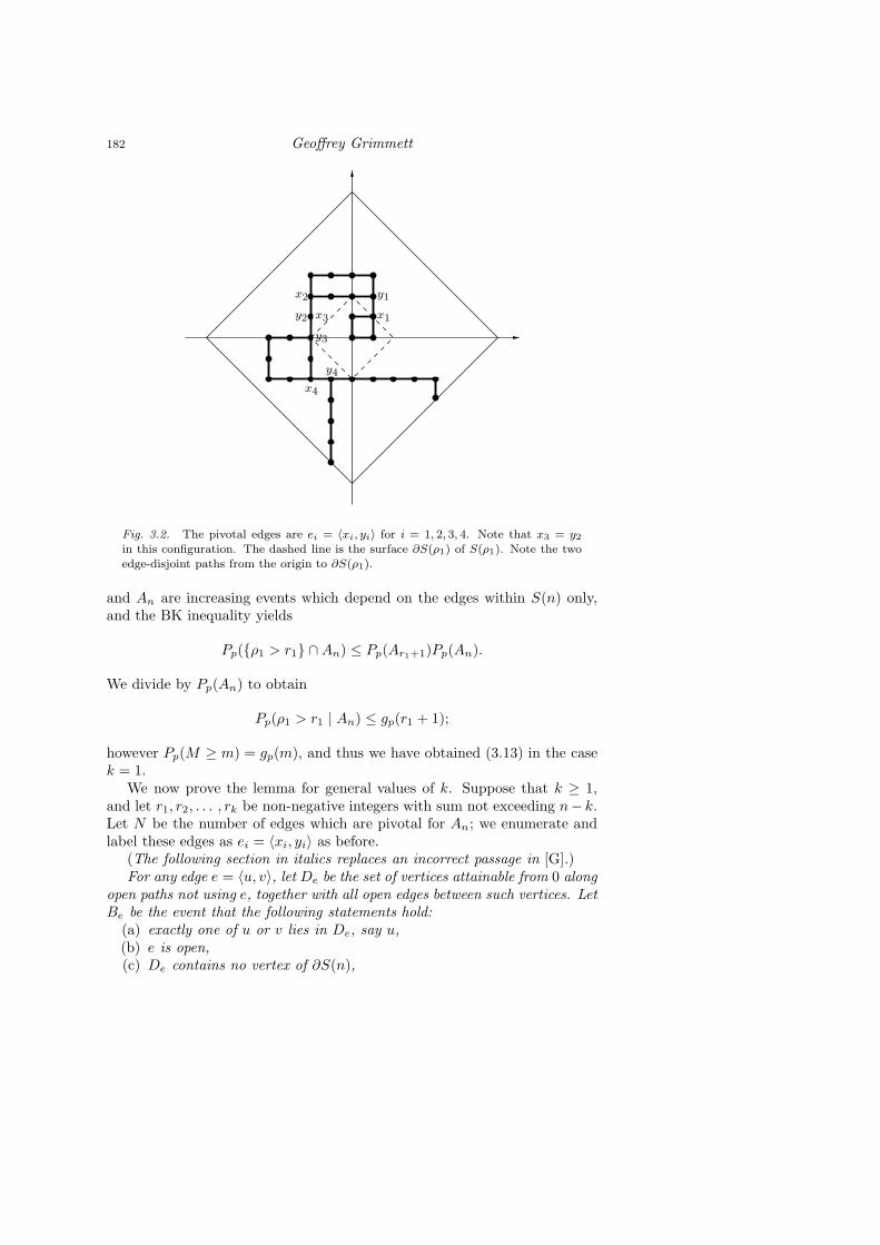
Suppose that the event An occurs, and denote by e1, e2, . . . , eN the (ran-dom) edges which are pivotal for An. Since An is increasing, each ej has theproperty that An occurs if and only if ej is open; thus all open paths fromthe origin to ∂S(n) traverse ej , for every j (see Figure 3.1). Let π be such anopen path; we assume that the edges e1, e2, . . . , eN have been enumerated inthe order in which they are traversed by π. A glance at Figure 3.1 confirmsthat this ordering is independent of the choice of π. We denote by xi theendvertex of ei encountered first by π, and by yi the other endvertex of ei.We observe that there exist at least two edge-disjoint open paths joining 0to x1, since, if two such paths cannot be found then, by Menger’s theorem(Wilson 19793, p. 126), there exists a pivotal edge in π which is encounteredprior to x1, a contradiction. Similarly, for 1 ≤ i < N , there exist at least twoedge-disjoint open paths joining yi to xi+1; see Figure 3.2. In the words ofthe discoverer of this proof, the open cluster containing the origin resemblesa chain of sausages.
As before, let M = maxk : Ak occurs be the radius of the largest ballwhose surface contains a vertex which is joined to the origin by an open path.We note that, if p < pc, then M has a non-defective distribution in that
3Reference [358].
Percolation and Disordered Systems 181
e2 e1
e3
0
e4
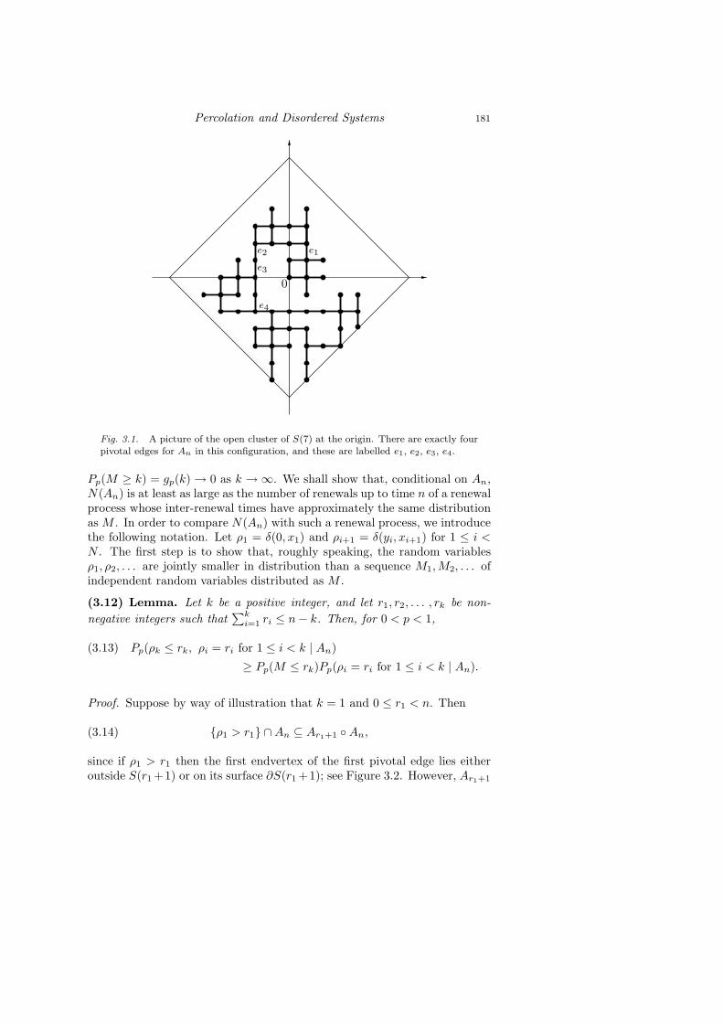
Fig. 3.1. A picture of the open cluster of S(7) at the origin. There are exactly fourpivotal edges for An in this configuration, and these are labelled e1, e2, e3, e4.
Pp(M ≥ k) = gp(k) → 0 as k → ∞. We shall show that, conditional on An,N(An) is at least as large as the number of renewals up to time n of a renewalprocess whose inter-renewal times have approximately the same distributionas M . In order to compare N(An) with such a renewal process, we introducethe following notation. Let ρ1 = δ(0, x1) and ρi+1 = δ(yi, xi+1) for 1 ≤ i <N . The first step is to show that, roughly speaking, the random variablesρ1, ρ2, . . . are jointly smaller in distribution than a sequence M1,M2, . . . ofindependent random variables distributed as M .
(3.12) Lemma. Let k be a positive integer, and let r1, r2, . . . , rk be non-
negative integers such that∑ki=1 ri ≤ n− k. Then, for 0 < p < 1,
(3.13) Pp(ρk ≤ rk, ρi = ri for 1 ≤ i < k | An)
≥ Pp(M ≤ rk)Pp(ρi = ri for 1 ≤ i < k | An).
Proof. Suppose by way of illustration that k = 1 and 0 ≤ r1 < n. Then
(3.14) ρ1 > r1 ∩An ⊆ Ar1+1 An,
since if ρ1 > r1 then the first endvertex of the first pivotal edge lies eitheroutside S(r1 +1) or on its surface ∂S(r1 +1); see Figure 3.2. However, Ar1+1
182 Geoffrey Grimmett
x2 y1
y2 x1x3
y3
y4
x4
Fig. 3.2. The pivotal edges are ei = 〈xi, yi〉 for i = 1, 2, 3, 4. Note that x3 = y2
in this configuration. The dashed line is the surface ∂S(ρ1) of S(ρ1). Note the twoedge-disjoint paths from the origin to ∂S(ρ1).
and An are increasing events which depend on the edges within S(n) only,and the BK inequality yields
Pp(ρ1 > r1 ∩An) ≤ Pp(Ar1+1)Pp(An).
We divide by Pp(An) to obtain
Pp(ρ1 > r1 | An) ≤ gp(r1 + 1);
however Pp(M ≥ m) = gp(m), and thus we have obtained (3.13) in the casek = 1.
We now prove the lemma for general values of k. Suppose that k ≥ 1,and let r1, r2, . . . , rk be non-negative integers with sum not exceeding n− k.Let N be the number of edges which are pivotal for An; we enumerate andlabel these edges as ei = 〈xi, yi〉 as before.
(The following section in italics replaces an incorrect passage in [G].)For any edge e = 〈u, v〉, let De be the set of vertices attainable from 0 along
open paths not using e, together with all open edges between such vertices. LetBe be the event that the following statements hold:
(a) exactly one of u or v lies in De, say u,(b) e is open,(c) De contains no vertex of ∂S(n),

Percolation and Disordered Systems 183
e
Fig. 3.3. A sketch of the event Be. The dashed line indicates that the only open‘exit’ from the interior is via the edge e. Note the existence of 3 pivotal edges for theevent that 0 is connected to an endvertex of e.
(d) the pivotal edges for the event 0 ↔ v are (in order) 〈x1, y1〉, 〈x2, y2〉,. . . , 〈xk−2, yk−2〉, 〈xk−1, yk−1〉 = e, where δ(yi−1, xi) = ri for 1 ≤ i <k, and y0 = 0.
We now define the event B =⋃eBe. For ω ∈ An ∩ B, there is a unique
e = e(ω) such that Be occurs.For ω ∈ B, we consider the set of vertices and open edges attainable along
open paths from the origin without using e = e(ω); to this graph we appende and its other endvertex v = yk−1, and we place a mark over yk−1 in orderto distinguish it from the other vertices. We denote by G = De the resulting(marked) graph, and we write y(G) for the unique marked vertex of G. Wecondition on G to obtain
Pp(An ∩B) =∑
Γ
Pp(B,G = Γ)Pp(An | B,G = Γ),
where the sum is over all possible values Γ of G. The final term in thissummation is the probability that y(Γ) is joined to ∂S(n) by an open pathwhich has no vertex other than y(Γ) in common with Γ. Thus, in the obviousterminology,
(3.15) Pp(An ∩B) =∑
Γ
Pp(B,G = Γ)Pp(y(Γ) ↔ ∂S(n) off Γ
).
184 Geoffrey Grimmett
Similarly,
Pp(ρk > rk ∩An ∩B)
=∑
Γ
Pp(B,G = Γ)Pp(ρk > rk ∩An | B,G = Γ)
=∑
Γ
Pp(B,G = Γ)
× Pp
(y(Γ) ↔ ∂S(rk + 1, y(Γ)) off Γ
y(Γ) ↔ ∂S(n) off Γ
).
We apply the BK inequality to the last term to obtain
Pp(ρk > rk ∩An ∩B)
(3.16)
≤∑
Γ
Pp(B,G = Γ)Pp(y(Γ) ↔ ∂S(n) off Γ
)
× Pp
(y(Γ) ↔ ∂S
(rk + 1, y(Γ)
)off Γ
)
≤ gp(rk + 1)Pp(An ∩B)
by (3.15) and the fact that, for each possible Γ,
Pp
(y(Γ) ↔ ∂S
(rk + 1, y(Γ)
)off Γ
)≤ Pp
(y(Γ) ↔ ∂S
(rk + 1, y(Γ)
))
= Pp(Ark+1)
= gp(rk + 1).
We divide each side of (3.16) by Pp(An ∩B) to obtain
Pp(ρk ≤ rk | An ∩B) ≥ 1 − gp(rk + 1),
throughout which we multiply by Pp(B | An) to obtain the result.
(3.17) Lemma. For 0 < p < 1, it is the case that
(3.18) Ep(N(An) | An
)≥ n∑n
i=0 gp(i)− 1.
Proof. It follows from Lemma (3.12) that
(3.19) Pp(ρ1 +ρ2 + · · ·+ρk ≤ n−k | An) ≥ P (M1 +M2 + · · ·+Mk ≤ n−k),
where k ≥ 1 and M1,M2, . . . is a sequence of independent random variablesdistributed as M . We defer until the end of this proof the minor chore of

Percolation and Disordered Systems 185
deducing (3.19) from (3.13). Now N(An) ≥ k if ρ1 + ρ2 + · · · + ρk ≤ n− k,so that
(3.20) Pp(N(An) ≥ k | An
)≥ P (M1 +M2 + · · · +Mk ≤ n− k).
A minor difficulty is that the Mi may have a defective distribution. Indeed,
P (M ≥ r) = gp(r)
→ θ(p) as r → ∞;
thus we allow the Mi to take the value ∞ with probability θ(p). On the otherhand, we are not concerned with atoms at ∞, since
P (M1 +M2 + · · · +Mk ≤ n− k) = P (M ′1 +M ′
2 + · · · +M ′k ≤ n),
where M ′i = 1 + minMi, n, and we work henceforth with these truncated
random variables. Summing (3.20) over k, we obtain
Ep(N(An) | An
)≥
∞∑
k=1
P (M ′1 +M ′
2 + · · · + M ′k ≤ n)(3.21)
=
∞∑
k=1
P (K ≥ k + 1)
= E(K) − 1,
where K = mink : M ′1 +M ′
2 + · · ·+M ′k > n. Let Sk = M ′
1 +M ′2 + · · ·+M ′
k,the sum of independent, identically distributed, bounded random variables.By Wald’s equation (see Chow and Teicher 19784, pp. 137, 150),
n < E(SK) = E(K)E(M ′1),
giving that
E(K) >n
E(M ′1)
=n
1 + E(minM1, n)=
n∑ni=0 gp(i)
since
E(minM1, n) =
n∑
i=1
P (M ≥ i) =
n∑
i=1
gp(i).
4Reference [106].

186 Geoffrey Grimmett
It remains to show that (3.19) follows from Lemma (3.12). We have that
Pp(ρ1 + ρ2 + · · · + ρk ≤ n− k | An)
=n−k∑
i=0
Pp(ρ1 + ρ2 + · · · + ρk−1 = i, ρk ≤ n− k − i | An)
≥n−k∑
i=0
P (M ≤ n− k − i)Pp(ρ1 + ρ2 + · · · + ρk−1 = i | An) by (3.13)
= Pp(ρ1 + ρ2 + · · · + ρk−1 +Mk ≤ n− k | An),
where Mk is a random variable which is independent of all edge-states inS(n) and is distributed as M . There is a mild abuse of notation here, sincePp is not the correct probability measure unless Mk is measurable on theusual σ-field of events, but we need not trouble ourselves overmuch aboutthis. We iterate the above argument in the obvious way to deduce (3.19),thereby completing the proof of the lemma.
The conclusion of Theorem (3.8) is easily obtained from this lemma, butwe delay this step until the end of the section. The proof of Theorem (3.4)proceeds by substituting (3.18) into (3.11) to obtain that, for 0 ≤ α < β ≤ 1,
gα(n) ≤ gβ(n) exp
(−∫ β
α
[n∑n
i=0 gp(i)− 1
]dp
).
It is difficult to calculate the integral in the exponent, and so we use theinequality gp(i) ≤ gβ(i) for p ≤ β to obtain
(3.22) gα(n) ≤ gβ(n) exp
(−(β − α)
[n∑n
i=0 gβ(i)− 1
]),
and it is from this relation that the conclusion of Theorem (3.4) will beextracted. Before continuing, it is interesting to observe that by combining(3.10) and (3.18) we obtain a differential-difference inequality involving thefunction
G(p, n) =n∑
i=0
gp(i);
rewriting this equation rather informally as a partial differential inequality,we obtain
(3.23)∂2G
∂p ∂n≥ ∂G
∂n
( nG
− 1).
Efforts to integrate this inequality directly have failed so far.

Percolation and Disordered Systems 187
Once we know that
Eβ(M) =∞∑
i=1
gβ(i) <∞ for all β < pc,
then (3.22) gives us that
gα(n) ≤ e−nψ(α) for all α < pc,
for some ψ(α) > 0, as required. At the moment we know rather less than thefinite summability of the gp(i) for p < pc, knowing only that gp(i) → 0 asi→ ∞. In order to estimate the rate at which gp(i) → 0, we shall use (3.22)as a mathematical turbocharger.
(3.24) Lemma. For p < pc, there exists δ(p) such that
(3.25) gp(n) ≤ δ(p)n−1/2 for n ≥ 1.
Once this lemma has been proved, the theorem follows quickly. To seethis, note that (3.25) implies the existence of ∆(p) <∞ such that
(3.26)
n∑
i=0
gp(i) ≤ ∆(p)n1/2 for p < pc.
Let α < pc, and find β such that α < β < pc. Substitute (3.26) with p = βinto (3.22) to find that
gα(n) ≤ gβ(n) exp
−(β − α)
(n1/2
∆(β)− 1
)
≤ exp
1 − (β − α)
∆(β)n1/2
.
Thus∞∑
n=1
gα(n) <∞ for α < pc,
and the theorem follows from the observations made prior to the statementof Lemma (3.24). We shall now prove this lemma.
Proof. First, we shall show the existence of a subsequence n1, n2, . . . alongwhich gp(n) approaches 0 rather quickly; secondly, we shall fill in the gaps inthis subsequence.

188 Geoffrey Grimmett
Fix β < pc and a positive integer n. Let α satisfy 0 < α < β and letn′ ≥ n; later we shall choose α and n′ explicitly in terms of β and n. From(3.22),
gα(n′) ≤ gβ(n′) exp
(1 − n′(β − α)
∑n′
i=0 gβ(i)
)(3.27)
≤ gβ(n) exp
(1 − n′(β − α)
∑n′
i=0 gβ(i)
)
since n ≤ n′. We wish to write the exponent in terms of gβ(n), and to thisend we shall choose n′ appropriately. We split the summation into two partscorresponding to i < n and i ≥ n, and we use the monotonicity of gβ(i) tofind that
1
n′
n′∑
i=0
gβ(i) ≤ 1
n′ngβ(0) + n′gβ(n)
≤ 3gβ(n) if n′ ≥ n⌊gβ(n)−1⌋.
We now define
(3.28) n′ = nγβ(n) where γβ(n) = ⌊gβ(n)−1⌋
and deduce from (3.27) that
(3.29) gα(n′) ≤ gβ(n) exp
(1 − β − α
3gβ(n)
).
Next we choose α by setting
(3.30) β − α = 3gβ(n)1 − log gβ(n).
Now gβ(m) → 0 as m → ∞, so that 0 < α < β if n has been picked largeenough; (3.29) then yields
(3.31) gα(n′) ≤ gβ(n)2.
This conclusion is the basic recursion step which we shall use repeatedly. Wehave shown that, for β < pc, there exists n0(β) such that (3.31) holds for alln ≥ n0(β) whenever n′ and α are given by (3.28) and (3.30), respectively.
Next, we fix p < pc and choose π such that p < π < pc. We now constructsequences (pi : i ≥ 0) of probabilities and (ni : i ≥ 0) of integers as follows.We set p0 = π and shall pick n0 later. Having found p0, p1, . . . , pi andn0, n1, . . . , ni, we define
(3.32) ni+1 = niγi and pi − pi+1 = 3gi(1 − log gi)

Percolation and Disordered Systems 189
where gi = gpi(ni) and γi = ⌊g−1
i ⌋. We note that ni ≤ ni+1 and pi > pi+1.The recursion (3.32) is valid so long as pi+1 > 0, and this is indeed the caseso long as n0 has been chosen to be sufficiently large. To see this we argue asfollows. From the definition of p0, . . . , pi and n0, . . . , ni and the discussionleading to (3.31), we find that
(3.33) gj+1 ≤ g2j for j = 0, 1, . . . , i− 1.
If a real sequence (xj : j ≥ 0) satisfies 0 < x0 < 1, xj+1 = x2j for j ≥ 0, then
it is easy to check that
s(x0) =
∞∑
j=0
3xj(1 − log xj) <∞,
and furthermore that s(x0) → 0 as x0 → 0. We may pick x0 sufficiently smallsuch that
(3.34) s(x0) ≤ π − p
and then we pick n0 sufficiently large that g0 = gπ(n0) < x0. Now h(x) =3x(1− logx) is an increasing function on [0, x0], giving from (3.32) and (3.33)that
pi+1 = pi − 3gi(1 − log gi)
= π −i∑
j=0
2gj(1 − log gj)
≥ π −∞∑
j=0
3xj(1 − log xj)
≥ p by (3.34).
Thus, by a suitable choice of n0 we may guarantee not only that pi+1 > 0 forall i but also that
p = limi→∞
pi
satisfies p ≥ p. Let us suppose that n0 has been chosen accordingly, so thatthe recursion (3.32) is valid and p ≥ p. We have from (3.32) and (3.33) that
nk = n0γ0γ1 . . . γk−1 for k ≥ 1
and
g2k−1 = gk−1gk−1(3.35)
≤ gk−1g2k−2 ≤ · · ·
≤ gk−1gk−2 . . . g1g20
≤ (γk−1γk−2 . . . γ0)−1g0
= δ2n−1k ,

190 Geoffrey Grimmett
where δ2 = n0g0.We are essentially finished. Let n > n0, and find an integer k such that
nk−1 ≤ n < nk; this is always possible since gk → 0 as k → ∞, and thereforenk−1 < nk for all large k. Then
gp(n) ≤ gpk−1(nk−1) since p ≤ pk−1
= gk−1
≤ δn−1/2k by (3.35)
≤ δn−1/2 since n < nk
as required. This is valid for n > n0, but we may adjust the constant δ sothat a similar inequality is valid for all n ≥ 1.
6.3 Ornstein–Zernike Decay
The connectivity function τp(x, y) = Pp(x ↔ y) decays exponentially whenp < pc, which is to say that the limits
(6.12) φ(p, x) = limn→∞
− 1
nlog τp(0, nx)
exist and satisfy φ(p, x) > 0 for 0 < p < pc and x ∈ Zd \ 0 (cf. Theorem6.2).
In one direction, this observation may lead to a study of the functionφ(p, ·). In another, one may ask for finer asymptotics in (6.12). We concen-trate on the case x = e1, and write φ(p) = φ(p, e1).
Theorem 6.13 (Ornstein–Zernike Decay). Suppose that 0 < p < pc.There exists a positive function A(p) such that
τp(0, ne1) =(1 + O(n−1)
) A(p)
n12 (d−1)
e−nφ(p) as n→ ∞.
The correction factor n− 12 (d−1) occurs similarly in many other disordered
systems, as was proposed by Ornstein and Zernike [300]. Theorem 6.13, andcertain extensions, was obtained for percolation by Campanino, Chayes, andChayes [85].

Percolation and Disordered Systems 191
7. SUPERCRITICAL PERCOLATION
7.1 Uniqueness of the Infinite Cluster
Let I be the number of infinite open clusters.
Theorem 7.1. For any p, either Pp(I = 0) = 1 or Pp(I = 1) = 1.
This result was proved first in [20], then more briefly in [145], and thedefinitive proof of Burton and Keane [82] appeared shortly afterwards. Thislast proof is short and elegant, and relies only on the zero–one law and alittle geometry.
Proof. Fix p ∈ [0, 1]. The sample space Ω = 0, 1E is a product space with anatural family of translations inherited from the translations of the lattice L
d.Furthermore, Pp is a product measure on Ω. Since I is a translation-invariantfunction on Ω, it is a.s. constant, which is to say that
(7.2) there exists k ∈ 0, 1, . . . ∪ ∞ such that Pp(I = k) = 1.
Naturally, the value of k depends on the choice of p. Next we show thatthe k in question satisfies k ∈ 0, 1,∞. Suppose (7.2) holds with some ksatisfying 2 ≤ k <∞. We may find a box B sufficiently large that
(7.3) Pp(B intersects two or more infinite clusters) > 12 .
By changing the states of edges in B (by making all such edges open, say) wecan decrease the number of infinite clusters (on the event in (7.3)). ThereforePp(I = k − 1) > 0, in contradiction of (7.2). Therefore we cannot have2 ≤ k <∞ in (7.2).
It remains to rule out the case k = ∞. Suppose that k = ∞. We willderive a contradiction by using a geometrical argument. We call a vertex xa trifurcation if:
(a) x lies in an infinite open cluster, and(b) the deletion of x splits this infinite cluster into exactly three disjoint
infinite clusters and no finite clusters,and we denote by Tx the event that x is a trifurcation. Now Pp(Tx) is constantfor all x, and therefore
(7.4)1
|B(n)| Ep( ∑
x∈B(n)
1Tx
)= Pp(T0).
(Recall that 1A denotes the indicator function of an event A.) It is usefulto know that the quantity Pp(T0) is strictly positive, and it is here that weuse the assumed multiplicity of infinite clusters. Since Pp(I = ∞) = 1 byassumption, we may find a box B(n) sufficiently large that it intersects at

192 Geoffrey Grimmett
Fig. 7.1. Take a box B which intersects at least three distinct infinite open clusters,and then alter the configuration inside B in order to create a configuration in which0 is a trifurcation.
least three distinct infinite clusters with probability at least 12 . By changing
the configuration inside B(n), we may turn the origin into a trifurcation (seeFigure 7.1). The corresponding set of configurations has strictly positiveprobability, so that Pp(T0) > 0 in (7.4).
Before turning to the geometry, we present a lemma concerning partitions.Let Y be a finite set with |Y | ≥ 3, and define a 3-partition Π = P1, P2, P3of Y to be a partition of Y into exactly three non-empty sets P1, P2, P3.For 3-partitions Π = P1, P2, P3 and Π′ = P ′
1, P′2, P
′3, we say that Π
and Π′ are compatible if there exists an ordering of their elements such thatP1 ⊇ P ′
2 ∪ P ′3 (or, equivalently, that P ′
1 ⊇ P2 ∪ P3). A collection P of 3-partitions is compatible if each pair therein is compatible.
Lemma 7.5. If P is a compatible family of distinct 3-partitions of Y , then|P| ≤ |Y | − 2.
Proof. There are several ways of doing this; see [82]. For any set Q of distinctcompatible 3-partitions of Y , we define an equivalence relation ∼ on Y byx ∼ y if, for all Π ∈ Q, x and y lie in the same element of Π. Write α(Q) forthe number of equivalence classes of ∼. Now, write P = (Π1,Π2, . . . ,Πm)in some order, and let αk = α(Π1,Π2, . . . ,Πk). Evidently α1 = 3 and, usingthe compatibility of Π1 and Π2, we have that α2 ≥ 4. By comparing Πr+1
with Π1,Π2, . . . ,Πr in turn, and using their compatibility, one sees thatα(Π1,Π2, . . . ,Πr+1) ≥ α(Π1,Π2, . . . ,Πr) + 1, whence αm ≥ α1 + (m− 1) =m+ 2. However αm ≤ |Y |, and the claim of the lemma follows.
Let K be a connected open cluster of B(n), and write ∂K = K ∩ ∂B(n).If x (∈ B(n − 1)) is a trifurcation in K, then the removal of x induces a3-partition ΠK(x) = P1, P2, P3 of ∂K with the properties that
(a) Pi is non-empty, for i = 1, 2, 3,(b) Pi is a subset of a connected subgraph of B(n)\x,(c) Pi = Pj in B(n), if i 6= j.

Percolation and Disordered Systems 193
x
x′
Fig. 7.2. Two trifurcations x and x′ belonging to a cluster K of B(n). They inducecompatible partitions of ∂K.
Furthermore, if x and x′ are distinct trifurcations of K ∩ B(n − 1), thenΠK(x) and ΠK(x′) are distinct and compatible; see Figure 7.2.
It follows by Lemma 7.5 that the number T (K) of trifurcations in K ∩B(n− 1) satisfies
T (K) ≤ |∂K| − 2.
We sum this inequality over all connected clusters of B(n), to obtain that
∑
x∈B(n−1)
1Tx≤ |∂B(n)|.
Take expectations, and use (7.4) to find that
|B(n− 1)|Pp(T0) ≤ |∂B(n)|,
which is impossible for large n since the left side grows as nd and the rightside as nd−1. This contradiction completes the proof.

194 Geoffrey Grimmett
7.2 Percolation in Slabs
Many results were proved for subcritical percolation under the hypothesisof ‘finite susceptibility’, i.e., that χ(p) = Ep|C| satisfies χ(p) < ∞. Sub-sequently, it was proved in [12, 267, 270] that this hypothesis is satisfiedwhenever p < pc. The situation was similar for supercritical percolation, thecorresponding hypothesis being that percolation occurs in slabs. We definethe slab of thickness k by
Sk = Zd−1 × 0, 1, . . . , k,
with critical probability pc(Sk); we assume here that d ≥ 3. The decreasinglimit pc(S) = limk→∞ pc(Sk) exists, and satisfies pc(S) ≥ pc. The hypoth-esis of ‘percolation in slabs’ is that p > pc(S). Here is an example of thehypothesis in action (cf. Theorem 6.2 and equation (6.8)).
Theorem 7.6. The limit
σ(p) = limn→∞
− 1
nlogPp(0 ↔ ∂B(n), |C| <∞)
exists. Furthermore σ(p) > 0 if p > pc(S).
This theorem asserts the exponential decay of a ‘truncated’ connectivityfunction when d ≥ 3. Corresponding results when d = 2 may be proved usingduality.
Proof. The existence of the limit is an exercise in subadditivity (see [94, G]),and we sketch here only a proof that σ(p) > 0. Assume that p > pc(S), sothat p > pc(Sk) for some k; choose k accordingly. Let Hn be the hyperplanecontaining all vertices x with x1 = n. It suffices to prove that
(7.7) Pp(0 ↔ Hn, |C| <∞) ≤ e−γn
for some γ = γ(p) > 0. Define the slabs
Ti = x ∈ Zd : (i− 1)k ≤ x1 < ik, 1 ≤ i < ⌊n/k⌋.
Any path from 0 to Hn must traverse every such slab. Since p > pc(Sk), eachslab a.s. contains an infinite open cluster. If 0 ↔ Hn and |C| < ∞, then allpaths from 0 to Hn must evade all such clusters. There are ⌊n/k⌋ slabs totraverse, and a price is paid for each. With a touch of rigour, this argumentimplies that
Pp(0 ↔ Hn, |C| <∞) ≤ 1 − θk(p)⌊n/k⌋
whereθk(p) = Pp(0 ↔ ∞ in Sk) > 0.
For more details, see [G].
Grimmett and Marstrand [164] proved that pc = pc(S), using ideas similarto those of [48, 49]. This was achieved via a ‘block construction’ whichappears to be central to a full understanding of supercritical percolation andto have further applications elsewhere. The details are presented next.

Percolation and Disordered Systems 195
7.3 Limit of Slab Critical Points
Material in this section is taken from [164]. We assume that d ≥ 3 and thatp is such that θ(p) > 0; under this hypothesis, we wish to gain some controlof the (a.s.) unique open cluster. In particular we shall prove the followingtheorem, in which pc(A) denotes the critical value of bond percolation on thesubgraph of Zd induced by the vertex set A. In this notation, pc = pc(Z
d).
Theorem 7.8. If F is an infinite connected subset of Zd with pc(F ) < 1,then for each η > 0 there exists an integer k such that
pc
(2kF +B(k)
)≤ pc + η.
Choosing F = Z2 × 0d−2, we have that 2kF + B(k) = x ∈ Zd : −k ≤xj ≤ k for 3 ≤ j ≤ d. The theorem implies that pc(2kF + B(k)) → pc ask → ∞, which is a stronger statement than the statement that pc = pc(S).
In the remainder of this section, we sketch the salient features of theblock construction necessary to prove the above theorem. This constructionmay be used directly to obtain further information concerning supercriticalpercolation.
The main idea involves working with a ‘block lattice’ each point of whichrepresents a large box of Ld, these boxes being disjoint and adjacent. In thisblock lattice, we declare a vertex to be ‘open’ if there exist certain open pathsin and near the corresponding box of Ld. We shall show that, with positiveprobability, there exists an infinite path of open vertices in the block lattice.Furthermore, this infinite path of open blocks corresponds to an infinite openpath of Ld. By choosing sufficiently large boxes, we aim to find such a pathwithin a sufficiently wide slab. Thus there is a probabilistic part of the proof,and a geometric part.
There are two main steps in the proof. In the first, we show the existenceof long finite paths. In the second, we show how to take such finite pathsand build an infinite cluster in a slab.
The principal parts of the first step are as follows. Pick p such thatθ(p) > 0.
1. Let ǫ > 0. Since θ(p) > 0, there exists m such that
Pp(B(m) ↔ ∞
)> 1 − ǫ.
This is elementary probability theory.2. Let n ≥ 2m, say, and let k ≥ 1. We may choose n sufficiently large to
ensure that, with probability at least 1− 2ǫ, B(m) is joined to at leastk points in ∂B(n).
3. By choosing k sufficiently large, we may ensure that, with probabilityat least 1 − 3ǫ, B(m) is joined to some point of ∂B(n), which is itselfconnected to a copy of B(m), lying ‘on’ the surface ∂B(n) and everyedge of which is open.

196 Geoffrey Grimmett
4. The open copy of B(m), constructed above, may be used as a ‘seed’ foriterating the above construction. When doing this, we shall need somecontrol over where the seed is placed. It may be shown that every faceof ∂B(n) contains (with large probability) a point adjacent to someseed, and indeed many such points.
Above is the scheme for constructing long finite paths, and we turn to thesecond step.
5. This construction is now iterated. At each stage there is a certain(small) probability of failure. In order that there be a strictly positiveprobability of an infinite sequence of successes, we iterate ‘in two in-dependent directions’. With care, one may show that the constructiondominates a certain supercritical site percolation process on L2.
6. We wish to deduce that an infinite sequence of successes entails aninfinite open path of Ld within the corresponding slab. There aretwo difficulties with this. First, since there is not total control of thepositions of the seeds, the actual path in Ld may leave every slab. Thismay be overcome by a process of ‘steering’, in which, at each stage,we choose a seed in such a position as to compensate for any earlierdeviation in space.
7. A larger problem is that, in iterating the construction, we carry withus a mixture of ‘positive’ and ‘negative’ information (of the form that‘certain paths exist’ and ‘others do not’). In combining events we can-not use the FKG inequality. The practical difficulty is that, althoughwe may have an infinite sequence of successes, there will generallybe breaks in any corresponding open route to ∞. This is overcome bysprinkling down a few more open edges, i.e., by working at edge-densityp+ δ where δ > 0, rather than at p.
In conclusion, we show that, if θ(p) > 0 and δ > 0, then there is (withlarge probability) an infinite (p+ δ)-open path in a slice of the form
Tk = x ∈ Zd : 0 ≤ xj ≤ k for j ≥ 3
where k is sufficiently large. This implies that p+δ > pc(T ) = limk→∞ pc(Tk)if p > pc, i.e., that pc ≥ pc(T ). Since pc(T ) ≥ pc by virtue of the fact thatTk ⊆ Zd for all k, we may conclude that pc = pc(T ), implying also thatpc = pc(S).
Henceforth we suppose that d = 3; similar arguments are valid whend > 3. We begin with some notation and two key lemmas. As usual, B(n) =[−n, n]3, and we shall concentrate on a special face of B(n),
F (n) = x ∈ ∂B(n) : x1 = n,
and indeed on a special ‘quadrant’ of F (n),
T (n) = x ∈ ∂B(n) : x1 = n, xj ≥ 0 for j ≥ 2.

Percolation and Disordered Systems 197
B(n) B(m)
T (m,n)
Fig. 7.3. An illustration of the event in (7.10). The hatched region is a copy ofB(m) all of whose edges are p-open. The central box B(m) is joined by a path tosome vertex in ∂B(n), which is in turn connected to a seed lying on the surface ofB(n).
For m,n ≥ 1, let
T (m,n) =2m+1⋃
j=1
je1 + T (n)
where e1 = (1, 0, 0) as usual.We call a box x+B(m) a seed if every edge in x+B(m) is open. We now
set
K(m,n) =x ∈ T (n) : 〈x, x+ e1〉 is open, and
x+ e1 lies in some seed lying within T (m,n).
The random set K(m,n) is necessarily empty if n < 2m.
Lemma 7.9. If θ(p) > 0 and η > 0, there exists m = m(p, η) and n = n(p, η)such that 2m < n and
(7.10) Pp(B(m) ↔ K(m,n) in B(n)
)> 1 − η.
The event in (7.10) is illustrated in Figure 7.3.
Proof. Since θ(p) > 0, there exists a.s. an infinite open cluster, whence
Pp(B(m) ↔ ∞
)→ 1 as m→ ∞.
We pick m such that
(7.11) Pp(B(m) ↔ ∞
)> 1 − (1
3η)24,
for a reason which will become clear later.

198 Geoffrey Grimmett
For n > m, let V (n) = x ∈ T (n) : x ↔ B(m) in B(n). Pick M suchthat
(7.12) pPp(B(m) is a seed
)> 1 − (1
2η)1/M .
We shall assume for simplicity that 2m+ 1 divides n+ 1 (and that 2m < n),and we partition T (n) into disjoint squares with side-length 2m. If |V (n)| ≥(2m + 1)2M then B(m) is joined in B(n) to at least M of these squares.Therefore, by (7.12),
Pp(B(m) ↔ K(m,n) in B(n)
)
≥
1 −[1 − pPp
(B(m) is a seed
)]MPp(|V (n)| ≥ (2m+ 1)2M
)(7.13)
≥ (1 − 12η)Pp
(|V (n)| ≥ (2m+ 1)2M
).
We now bound the last probability from below. Using the symmetries ofL3 obtained by reflections in hyperplanes, we see that the face F (n) comprisesfour copies of T (n). Now ∂B(n) has six faces, and therefore 24 copies of T (n).By symmetry and the FKG inequality,
(7.14) Pp(|U(n)| < 24(2m+ 1)2M
)≥ Pp
(|V (n)| < (2m+ 1)2M
)24
where U(n) = x ∈ ∂B(n) : x ↔ B(m) in B(n). Now, with l = 24(2m +1)2M ,
(7.15) Pp(|U(n)| < l
)≤ Pp
(|U(n)| < l, B(m) ↔ ∞
)+ Pp
(B(m) = ∞
),
and
Pp(|U(n)| < l, B(m) ↔ ∞
)≤ Pp
(1 ≤ |U(n)| < l
)(7.16)
≤ (1 − p)−3lPp(U(n+ 1) = ∅, U(n) 6= ∅)
→ 0 as n→ ∞.
(Here we use the fact that U(n + 1) = ∅ if every edge exiting ∂B(n) fromU(n) is closed.)
By (7.14)–(7.16) and (7.11),
Pp(|V (n)| < (2m+ 1)2M
)≤ Pp
(|U(n)| < l
)1/24 ≤(an + (1
3η)24)1/24
where an → 0 as n→ ∞. We pick n such that
Pp(|V (n)| < (2m+ 1)2M
)≤ 1
2η,

Percolation and Disordered Systems 199
B(n)
R
Fig. 7.4. An illustration of Lemma 7.17. The hatched regions are copies of B(m)all of whose edges are p-open. The central box B(m) lies within some (dotted) regionR. Some vertex in R is joined by a path to some vertex in ∂B(n), which is in turnconnected to a seed lying on the surface of B(n).
and the claim of the lemma follows by (7.13).
Having constructed open paths from B(m) to K(m,n), we shall need torepeat the construction, beginning instead at an appropriate seed in K(m,n).This is problematic, since we have discovered a mixture of information, someof it negative, about the immediate environs of such seeds. In order to over-come the effect of such negative information, we shall work at edge-densityp+ δ rather than p. In preparation, let (X(e) : e ∈ Ed) be independent ran-dom variables having the uniform distribution on [0, 1], and let ηp(e) be theindicator function that X(e) < p; recall Section 2.3. We say that e is p-openif X(e) < p and p-closed otherwise, and we denote by P the appropriateprobability measure.
For any subset V of Z3, we define the exterior boundary ∆V and exterioredge-boundary ∆eV by
∆V = x ∈ Z3 : x 6∈ V, x ∼ y for some y ∈ V ,
∆eV = 〈x, y〉 : x ∈ V, y ∈ ∆V, x ∼ y.
We write EV for the set of all edges of L3 joining pairs of vertices in V .
We shall make repeated use of the following lemma5, which is illustratedin Figure 7.4.
5This lemma is basically Lemma 6 of [164], the difference being that [164] was addressedat site percolation. R. Meester and J. Steif have kindly pointed out that, in the case ofsite percolation, a slightly more general lemma is required than that presented in [164].The following remarks are directed at the necessary changes to Lemma 6 of [164], and theyuse the notation of [164]. The proof of the more general lemma is similar to that of theoriginal version. The domain of β is replaced by a general subset S of B(n) \ T (n), andG is the event there exists a path in B(n) from S to K(m, n), this path being p-open inB(n) \ S and (β(u) + δ)-open at its unique vertex u ∈ S. In applying the lemma justafter (4.10) of [164], we take S = ∆C2 ∩ B(n) (and similarly later).

200 Geoffrey Grimmett
Lemma 7.17. If θ(p) > 0 and ǫ, δ > 0, there exist integers m = m(p, ǫ, δ)and n = n(p, ǫ, δ) such that 2m < n and with the following property. LetR be such that B(m) ⊆ R ⊆ B(n) and (R ∪ ∆R) ∩ T (n) = ∅, and letβ : ∆eR ∩ EB(n) → [0, 1 − δ]. Define the events
G = there exists a path joining R to K(m,n), this path being p-open
outside ∆eR and (β(e) + δ)-open at its unique edge e lying in ∆eR,H = e is β(e)-closed for all e ∈ ∆eR ∩ EB(n).
Then P (G | H) > 1 − ǫ.
Proof. Assume that θ(p) > 0, and let ǫ, δ > 0. Pick an integer t so large that
(7.18) (1 − δ)t < 12ǫ
and then choose η (> 0) such that
(7.19) η < 12ǫ(1 − p)t.
We apply Lemma 7.9 with this value of η, thereby obtaining integers m,nsuch that 2m < n and
(7.20) Pp(B(m) ↔ K(m,n) in B(n)
)> 1 − η.
Let R and β satisfy the hypotheses of the lemma. Since any path fromB(m) to K(m,n) contains a path from ∂R to K(m,n) using no edges of ER,we have that
(7.21) Pp(∂R↔ K(m,n) in B(n)
)> 1 − η.
Let K ⊆ T (n), and let U(K) be the set of edges 〈x, y〉 of B(n) such that(i) x ∈ R, y 6∈ R, and
(ii) there is an open path joining y to K, using no edges of ER ∪ ∆eR.We wish to show that U(K) must be large if Pp(∂R ↔ K in B(n)) is large.The argument centres on the fact that every path from ∂R to K passesthrough U(K); if U(K) is ‘small’ then there is substantial uncertainty forthe occurrence of the event ∂R ↔ K in B(n), implying that this eventcannot have probability near 1. More rigorously,
Pp(∂R = K in B(n)
)= Pp(all edges in U(K) are closed)
(7.22)
≥ (1 − p)tPp(|U(K)| ≤ t
).

Percolation and Disordered Systems 201
We may apply this with K = K(m,n), since K(m,n) is defined on the set ofedges exterior to B(n). Therefore, by (7.21), (7.22), and (7.19),
Pp
(|U(K(m,n)
)∣∣> t)≥ 1 − (1 − p)−tPp
(∂R = K(m,n) in B(n)
)(7.23)
≥ 1 − (1 − p)−tη > 1 − 12ǫ.
We now couple together the percolation processes with different valuesof p on the same probability space, as described in Section 2.3 and justprior to the statement of Lemma 7.17. We borrow the notation and resultsderived above by specialising to the p-open edges. Conditional on the setU = U(K(m,n)), the values of X(e), for e ∈ U , are independent and uniformon [0, 1]. Therefore
P(
every e in U is (β(e) + δ)-closed, |U | > t∣∣∣H)≤ (1 − δ)t,
whence, using (7.18) and (7.23),
P(
some e in U is (β(e) + δ)-open∣∣∣H)≥ P (|U | > t | H) − (1 − δ)t
= Pp(|U | > t) − (1 − δ)t
≥ (1 − 12ǫ) − 1
2ǫ,
and the lemma is proved.
This completes the two key geometrical lemmas. In moving to the secondpart of the proof, we shall require a method for comparison of a ‘dependent’process and a site percolation process. The argument required at this stageis as follows.
Let F be an infinite connected subset of Ld for which the associated(site) critical probability satisfies pc(F, site) < 1, and let Z(x) : x ∈ F berandom variables taking values in [0, 1]. We construct a connected subset ofF in the following recursive manner. Let e(1), e(2), . . . be a fixed orderingof the edges of the graph induced by F . Let x1 ∈ F , and define the orderedpair S1 = (A1, B1) of subsets of F by
S1 =
(x1,∅) if Z(x1) = 1
(∅, x1) if Z(x1) = 0.
Having defined S1, S2, . . . , St = (At, Bt), for t ≥ 1, we define St+1 as follows.Let f be the earliest edge in the fixed ordering of the e(i) with the propertythat one endvertex, xt+1 say, lies in At and the other endvertex lies outsideAt ∪Bt. Then we declare
St+1 =
(At ∪ xt+1, Bt) if Z(xt+1) = 1,
(At, Bt ∪ xt+1) if Z(xt+1) = 0.
If no such edge f exists, we declare St+1 = St. The sets At, Bt are non-decreasing, and we set A∞ = limt→∞ At, B∞ = limt→∞Bt. Think aboutA∞ as the ‘occupied cluster’ at x1, and B∞ as its external boundary.

202 Geoffrey Grimmett
Lemma 7.24. Suppose there exists a constant γ such that γ > pc(F, site)and
(7.25) P(Z(xt+1) = 1
∣∣S1, S2, . . . , St)≥ γ for all t.
Then P (|A∞| = ∞) > 0.
We omit a formal proof of this lemma (but see [164]). Informally, (7.25)implies that, uniformly in the past history, the chance of extending At exceedsthe critical value of a supercritical site percolation process on F . ThereforeA∞ stochastically dominates the open cluster at x1 of a supercritical site per-colation cluster. The latter cluster is infinite with strictly positive probability,whence P (|A∞| = ∞) > 0.
Having established the three basic lemmas, we turn to the constructionitself. Recall the notation and hypotheses of Theorem 7.8. Let 0 < η < pc,and choose
(7.26) p = pc + 12η, δ = 1
12η, ǫ = 124
(1 − pc(F, site)
).
Note that pc(F, site) < 1 since by assumption pc(F ) = pc(F, bond) < 1(cf. Theorem 5.13). Since p > pc, we have that θ(p) > 0, and we applyLemma 7.17 with the above ǫ, δ to find corresponding integers m,n. Wedefine N = m + n + 1, and we shall define a process on the blocks of Z3
having side-length 2N .Consider the set 4Nx : x ∈ Zd of vertices, and the associated boxes
Bx(N) = 4Nx + B(N) : x ∈ Zd; these boxes we call site-boxes . A pairBx(N), By(N) of site-boxes is deemed adjacent if x and y are adjacent inLd. Adjacent site-boxes are linked by bond-boxes , i.e., boxes Nz + B(N)for z ∈ Zd exactly one component of which is not divisible by 4. If thisexceptional component of z is even, the box Nz +B(N) is called a half-waybox. See Figure 7.5.
We shall examine site-boxes one by one, declaring each to be ‘occupied’ or‘unoccupied’ according to the existence (or not) of certain open paths. Twoproperties of this construction will emerge.
(a) For each new site-box, the probability that it is occupied exceeds thecritical probability of a certain site percolation process. This will implythat, with strictly positive probability, there is an infinite occupiedpath of site-boxes.
(b) The existence of this infinite occupied path necessarily entails an infi-nite open path of Ld lying within some restricted region.
The site-boxes will be examined in sequence, the order of this sequence be-ing random, and depending on the past history of the process. Thus, therenormalisation is ‘dynamic’ rather than ‘static’.
As above, let F be an infinite connected subset of Zd; we shall assume forneatness that F contains the origin 0 (otherwise, translate F accordingly).As above, let e(1), e(2), . . . be a fixed ordering of the edges joining vertices in

Percolation and Disordered Systems 203
Fig. 7.5. The hatched squares are site-boxes, and the dotted squares are half-wayboxes. Each box has side-length 2N .
F . We shall examine the site-boxes Bx(N), for x ∈ F , and determine theirstates. This we do according to the algorithm sketched before Lemma 7.24,for appropriate random variables Z(x) to be described next.
We begin at the origin, with the site-box B0(N) = B(N). Once we haveexplained what is involved in determining the state of B0(N), most of thework will have been done. (The event B0(N) is occupied is sketched inFigure 7.7.)
Note that B(m) ⊆ B(N), and say that ‘the first step is successful’ if everyedge in B(m) is p-open, which is to say that B(m) is a ‘seed’. (Recall that pand other parameters are given in (7.26).) At this stage we write E1 for theset of edges of B(m).
In the following sequential algorithm, we shall construct an increasing se-quence E1, E2, . . . of edge-sets. At each stage k, we shall acquire informationabout the values of X(e) for certain e ∈ E3 (here, the X(e) are indepen-dent uniform [0, 1]-valued random variables, as usual). This information weshall record in the form ‘each e is βk(e)-closed and γk(e)-open’ for suitablefunctions βk, γk : E3 → [0, 1] satisfying
(7.27) βk(e) ≤ βk+1(e), γk(e) ≥ γk+1(e), for all e ∈ E3.
Having constructed E1, above, we set
β1(e) = 0 for all e ∈ E3,(7.28)
γ1(e) =
p if e ∈ E1,
1 otherwise.(7.29)

204 Geoffrey Grimmett
Fig. 7.6. An illustration of the first two steps in the construction of the event0 is occupied, when these steps are successful. Each hatched square is a seed.
Since we are working with edge-sets Ej rather than with vertex-sets, itwill be useful to have some corresponding notation. Two edges e, f are calledadjacent , written e ≈ f , if they have exactly one common endvertex. Thisadjacency relation defines a graph. Paths in this graph are said to be α-openif X(e) < α for all e lying in the path. The exterior edge-boundary ∆eE ofan edge-set E is the set of all edges f ∈ E3 \ E such that f ≈ e for somee ∈ E.
For j = 1, 2, 3 and σ = ±, let Lσj be an automorphism of L3 which
preserves the origin and maps e1 = (1, 0, 0) onto σej ; we insist that L+1 is the
identity. We now define E2 as follows. Consider the set of all paths π lyingwithin the region
B′1 = B(n) ∪
⋃
1≤j≤3σ=±
Lσj(T (m,n)
)
such that(a) the first edge f of π lies in ∆eE1 and is (β1(f) + δ)-open, and(b) all other edges lie outside E1 ∪ ∆eE1 and are p-open.
We define E2 = E1 ∪ F1 where F1 is the set of all edges in the union of suchpaths π. We say that ‘the second step is successful’ if, for each j = 1, 2, 3and σ = ±, there is an edge in E2 having an endvertex in Kσ
j (m,n), where
Kσj (m,n) =
z ∈ Lσj
(T (n)
):〈z, z + σej〉 is p-open, and z + σej lies
in some seed lying within Lσj(T (m,n)
).
The corresponding event is illustrated in Figure 7.6.

Percolation and Disordered Systems 205
Next we estimate the probability that the second step is successful, condi-tional on the first step being successful. Let G be the event that there exists apath in B(n)\B(m) from ∂B(m) to K(m,n), every edge e of which is p-openoff ∆eE1 and whose unique edge f in ∆eE1 is (β1(f) + δ)-open. We writeGσj for the corresponding event with K(m,n) replaced by Lσj (K(m,n)). Wenow apply Lemma 7.17 with R = B(m) and β = β1 to find that
P(Gσj∣∣B(m) is a seed
)> 1 − ǫ for j = 1, 2, 3, σ = ±.
Therefore
(7.30) P(Gσj occurs for all j, σ
∣∣B(m) is a seed)> 1 − 6ǫ,
so that the second step is successful with conditional probability at least1 − 6ǫ.
If the second step is successful, then we update the β, γ functions accord-ingly, setting
β2(e) =
β1(e) if e 6∈ EB′1,
β1(e) + δ if e ∈ ∆eE1\E2,
p if e ∈ ∆eE2\∆eE1,
0 otherwise,
(7.31)
γ2(e) =
γ1(e) if e ∈ E1,
β1(e) + δ if e ∈ ∆eE1 ∩ E2,
p if e ∈ E2\(E1 ∪ ∆eE1),
1 otherwise.
(7.32)
Suppose that the first two steps have been successful. We next aim tolink the appropriate seeds in each Lσj (T (m,n)) to a new seed lying in thebond-box 2σNej +B(N), i.e., the half-way box reached by exiting the originin the direction σej . If we succeed with each of the six such extensions,then we terminate this stage of the process, and declare the vertex 0 of therenormalised lattice to be occupied ; such success constitutes the definition ofthe term ‘occupied’. See Figure 7.7.
We do not present all the details of this part of the construction, sincethey are very similar to those already described. Instead we concentrateon describing the basic strategy, and discussing any novel aspects of theconstruction. First, let B2 = b2 +B(m) be the earliest seed (in some orderingof all copies of B(m)) all of whose edges lie in E2 ∩ ET (m,n). We now try toextend E2 to include a seed lying within the bond-box 2Ne1 +B(N). ClearlyB2 ⊆ Ne1 + B(N). In performing this extension, we encounter a ‘steering’problem. It happens (by construction) that all coordinates of b2 are positive,implying that b2 + T (m,n) is not a subset of 2Ne1 + B(N). We therefore

206 Geoffrey Grimmett
Fig. 7.7. An illustration of the event 0 is occupied. Each black square is a seed.
replace b2 + T (m,n) by b2 + T ∗(m,n) where T ∗(m,n) is given as follows.Instead of working with the ‘quadrant’ T (n) of the face F (n), we use the set
T ∗(n) =x ∈ ∂B(n) : x1 = n, xj ≤ 0 for j = 2, 3
.
We then define
T ∗(m,n) =
2m+1⋃
j=1
je1 + T ∗(n),
and obtain that b2 + T ∗(m,n) ⊆ 2Ne1 + B(N). We now consider the set ofall paths π lying within the region
B′2 = b2 + B(n) ∪ T ∗(m,n)
such that:(a) the first edge f of π lies in ∆eE2 and is (β2(f) + δ)-open, and(b) all other edges lie outside E2 ∪ ∆eE2 and are p-open.
We set E3 = E2 ∪ F2 where F2 is the set of all edges lying in the union ofsuch paths. We call this step successful if E3 contains an edge having anendvertex in the set
b2 +K∗(m,n) =z ∈ b2 + T ∗(m,n) : 〈z, z + e1〉 is p-open, z + e1
lies in some seed lying in b2 + T ∗(m,n).
Using Lemma 7.17, the (conditional) probability that this step is successfulexceeds 1 − ǫ.

Percolation and Disordered Systems 207
Fig. 7.8. Two adjacent site-boxes both of which are occupied. The constructionbegan with the left site-box B0(N) and has been extended to the right site-boxBe1 (N). The black squares are seeds, as before.
We perform similar extensions in each of the other five directions exitingB0(N). If all are successful, we declare 0 to be occupied . Combining theabove estimates of success, we find that
P (0 is occupied | B(m) is a seed) > (1 − 6ǫ)(1 − ǫ)6 > 1 − 12ǫ
(7.33)
= 12
(1 + pc(F, site)
)
by (7.26).If 0 is not occupied, we end the construction. If 0 is occupied, then this
has been achieved after the definition of a set E8 of edges. The correspondingfunctions β8, γ8 are such that
(7.34) β8(e) ≤ γ8(e) ≤ p+ 6δ for e ∈ E8;
this follows since no edge lies in more than 7 of the copies of B(n) usedin the repeated application of Lemma 7.17. Therefore every edge of E8 is(p+ η)-open, since δ = 1
12η (see (7.26)).The basic idea has been described, and we now proceed similarly. Assume
0 is occupied, and find the earliest edge e(r) induced by F and incident withthe origin; we may assume for the sake of simplicity that e(r) = 〈0, e1〉. Wenow attempt to link the seed b3 +B(m), found as above inside the half-waybox 2Ne1 +B(N), to a seed inside the site-box 4Ne1 +B(N). This is donein two steps of the earlier kind. Having found a suitable seed inside the newsite-box 4Ne1 + B(N), we attempt to branch-out in the other 5 directionsfrom this site-box. If we succeed in finding seeds in each of the correspondinghalf-way boxes, then we declare the vertex e1 of the renormalised lattice tobe occupied. As before, the (conditional) probability that e1 is occupied

208 Geoffrey Grimmett
Fig. 7.9. The central seed is B(m), and the connections represent (p+η)-open pathsjoining seeds within the site-boxes.
is at least 12 (1 + pc(F, site)), and every edge in the ensuing construction is
(p+ η)-open. See Figure 7.8.Two details arise at this and subsequent stages, each associated with
‘steering’. First, if b3 = (α1, α2, α3) we concentrate on the quadrant Tα(n)of ∂B(n) defined as the set of x ∈ ∂B(n) for which xjαj ≤ 0 for j = 2, 3 (sothat xj has the opposite sign to αj). Having found such a Tα(n), we defineT ∗α(m,n) accordingly, and look for paths from b3 + B(m) to b3 + T ∗
α(m,n).This mechanism guarantees that any variation in b3 from the first coordinateaxis is (at least partly) compensated for at the next step.
A further detail arises when branching out from the seed b∗+B(m) reachedinside 4Ne1+B(N). In finding seeds lying in the new half-way boxes abutting4Ne1+B(N), we ‘steer away from the inlet branch’, by examining seeds lyingon the surface of b∗ + B(n) with the property that the first coordinates oftheir vertices are not less than that of b∗. This process guarantees that theseseeds have not been examined previously.
We now continue to apply the algorithm presented before Lemma 7.24.At each stage, the chance of success exceeds γ = 1
2 (1 + pc(F, site)). Sinceγ > pc(F, site), we have from Lemma 7.24 that there is a strictly positiveprobability that the ultimate set of occupied vertices of F (i.e., renormalisedblocks of L3) is infinite. Now, on this event, there must exist an infinite(p+ η)-open path of L3 corresponding to the enlargement of F . This infiniteopen path must lie within the enlarged set 4NF + B(2N), implying thatpc + η ≥ pc(4NF + B(2N)), as required for Theorem 7.9. See Figure 7.9.The proof is complete.

Percolation and Disordered Systems 209
7.4 Percolation in Half-Spaces
In the last section, we almost succeeded in proving that θ(pc) = 0 whend ≥ 3. The reason for this statement is as follows. Suppose θ(p) > 0 andη > 0. There is effectively defined in Section 7.3 an event A living in a finitebox B such that
(a) Pp(A) > 1 − ǫ, for some prescribed ǫ > 0,(b) the fact (a) implies that θ(p+ η) > 0.
Suppose that we could prove this with η = 0, and that θ(pc) > 0. ThenPpc(A) > 1 − ǫ, which implies by continuity that Pp′(A) > 1 − ǫ for somep′ < pc, and therefore θ(p′) > 0 by (b). This would contradict the definitionof pc, whence we deduce by contradiction that θ(pc) = 0.
The fact that η is strictly positive is vital for the construction, sincewe need to ‘spend some extra money’ in order to compensate for negativeinformation acquired earlier in the construction. In a slightly different setting,no extra money is required.
Let H = 0, 1, . . . × Zd−1 be a half-space when d ≥ 3, and write pc(H)for its critical probability. It follows from Theorem 7.8 that pc(H) = pc, sinceH contains slabs of all thicknesses. Let
θH(p) = Pp(0 ↔ ∞ in H).
Theorem 7.35. We have that θH(pc) = 0.
The proof is not presented here, but may be found in [48, 49]. It is closelyrelated to that presented in Section 7.3, but with some crucial differences.The construction of blocks is slightly more complicated, owing to the lackof symmetry of H, but there are compensating advantages of working in ahalf-space. For amusement, we present in Figure 7.10 two diagrams (relevantto the argument of [49]) depicting the necessary constructions.
As observed in Section 3.3, such a conclusion for half-spaces has a strikingimplication for the conjecture that θ(pc) = 0. If θ(pc) > 0, then there existsa.s. a unique infinite open cluster in Zd, which is a.s. partitioned into (only)finite clusters by any division of Z
d into two half-spaces.
7.5 Percolation Probability
Although the methods of Chapter 6 were derived primarily in order to studysubcritical percolation, they involve a general inequality of wider use, namely
g′π(n) ≥ gπ(n)
(n∑n
i=0 gπ(i)− 1
)
where gπ(n) = Pπ(0 ↔ ∂Sn); see equations (3.10) and (3.18) in Section 6.We argue loosely as follows. Clearly gπ(n) → θ(π) as n→ ∞, whence (crossyour fingers here)
θ′(π) ≥ θ(π)
(1
θ(π)− 1
)
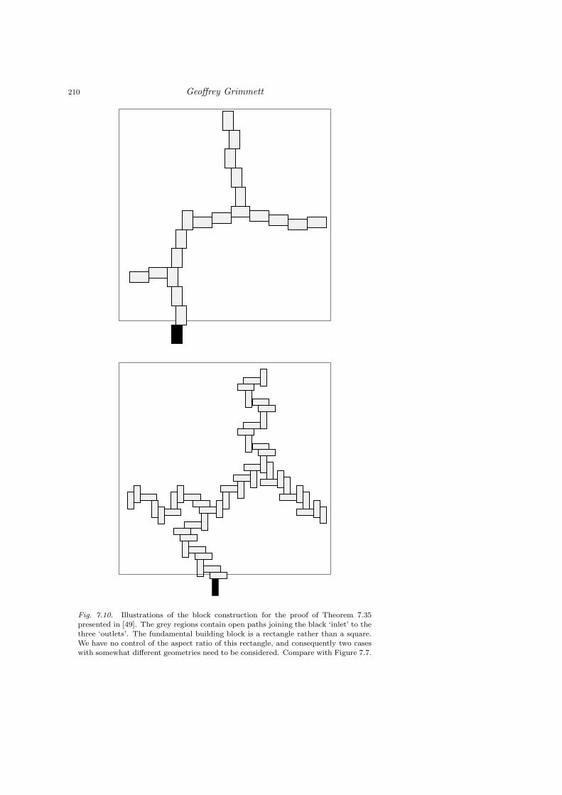
210 Geoffrey Grimmett
Fig. 7.10. Illustrations of the block construction for the proof of Theorem 7.35presented in [49]. The grey regions contain open paths joining the black ‘inlet’ to thethree ‘outlets’. The fundamental building block is a rectangle rather than a square.We have no control of the aspect ratio of this rectangle, and consequently two caseswith somewhat different geometries need to be considered. Compare with Figure 7.7.

Percolation and Disordered Systems 211
orθ′(π) + θ(π) ≥ 1.
Integrate this over the interval (pc, p) to obtain
θ(p)ep − θ(pc)epc ≥ ep − epc , pc ≤ p,
whence it is an easy exercise to show that
(7.36) θ(p) − θ(pc) ≥ a(p− pc), pc ≤ p,
for some positive constant a. The above argument may be made rigorous.Differential inequalities of the type above are used widely in percolation
and disordered systems.
7.6 Cluster-Size Distribution
When p < pc, the tail of the cluster-size |C| decays exponentially. Expo-nential decay is not correct when p > pc, but rather ‘stretched exponentialdecay’.
Theorem 7.37. Suppose pc < p < 1. There exist positive constants α(p),β(p) such that, for all n,
(7.38) exp(−αn(d−1)/d
)≤ Pp(|C| = n) ≤ exp
(−βn(d−1)/d
).
See [G] for a proof of this theorem. The reason for the power n(d−1)/d
is roughly as follows. It is thought that a large finite cluster is most likelycreated as a cluster of compact shape, all of whose boundary edges are closed.Now, if a ball has volume n, then its surface area has order n(d−1)/d. Theprice paid for having a surface all of whose edges are closed is (1−p)m wherem is the number of such edges. By the above remark, m should have ordern(d−1)/d, as required for (7.38).
It is believed that the limit
(7.39) γ(p) = limn→∞
− 1
n(d−1)/dlogPp(|C| = n)
exists, but no proof is known.Much more is known in two dimensions than for general d. The size and
geometry of large finite clusters have been studied in detail in [37], where itwas shown that such clusters may be approximated by the so called ‘Wulffshape’. This work includes a proof of the existence of the limit in (7.39) whend = 2.

212 Geoffrey Grimmett
8. CRITICAL PERCOLATION
8.1 Percolation Probability
The next main open question is to verify the following.
Conjecture 8.1. We have that θ(pc) = 0.
This is known to hold when d = 2 (using results of Harris [182], seeTheorem 9.1) and for sufficiently large values of d (by work of Hara andSlade [179, 180]), currently for d ≥ 19. The methods of Hara and Slademight prove feasible for values of d as small as 6 or 7, but not for smaller d.Some new idea is needed for the general conclusion. As remarked in Section7.4, we need to rule out the remaining theoretical possibility that there is aninfinite cluster in Zd when p = pc, but no infinite cluster in any half-space.
8.2 Critical Exponents
Macroscopic functions, such as the percolation probability, have a singularityat p = pc, and it is believed that there is ‘power law behaviour’ at and nearthis singularity. The nature of the singularity is supposed to be canonical,in that it is expected to have certain general features in common with phasetransitions in other physical systems. These features are sometimes referredto as ‘scaling theory’ and they relate to ‘critical exponents’.
There are two sets of critical exponents, arising firstly in the limit asp→ pc, and secondly in the limit over increasing distances when p = pc. Wesummarise the notation in Table 8.1.
The asymptotic relation ≈ should be interpreted loosely (perhaps via log-arithmic asymptotics). The radius of C is defined by rad(C) = maxn : 0 ↔∂B(n). The limit as p→ pc should be interpreted in a manner appropriatefor the function in question (for example, as p ↓ pc for θ(p), but as p → pc
for κ(p)).There are eight critical exponents listed in Table 8.1, denoted α, β, γ,
δ, ν, η, ρ, ∆, but there is no general proof of the existence of any of theseexponents.
8.3 Scaling Theory
In general, the eight critical exponents may be defined for phase transitionsin a quite large family of physical systems. However, it is not believed thatthey are independent variables, but rather that they satisfy the following:
2 − α = γ + 2β = β(δ + 1),
(8.2) Scaling relations
∆ = δβ,
γ = ν(2 − η),
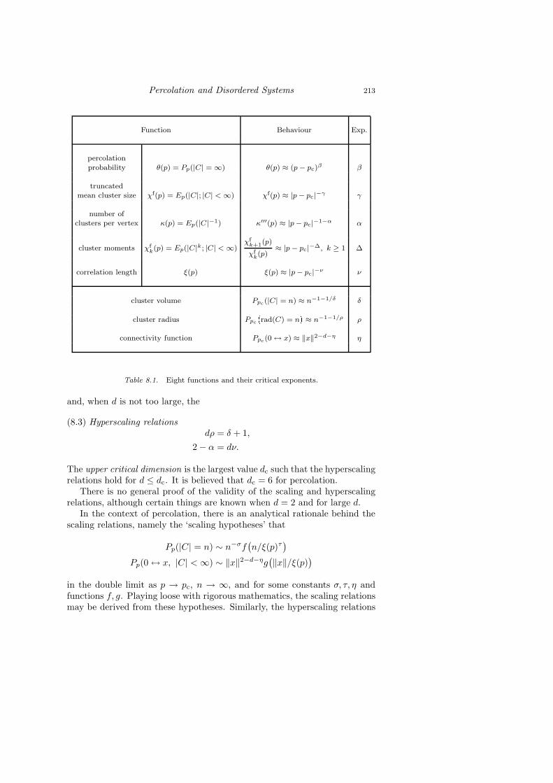
Percolation and Disordered Systems 213
Function Behaviour Exp.
percolation
probability θ(p) = Pp(|C| = ∞) θ(p) ≈ (p − pc)β β
truncatedmean cluster size χf(p) = Ep(|C|; |C| < ∞) χf(p) ≈ |p − pc|−γ γ
number ofclusters per vertex κ(p) = Ep(|C|−1) κ′′′(p) ≈ |p − pc|−1−α α
cluster moments χfk(p) = Ep(|C|k; |C| < ∞)
χfk+1
(p)
χfk(p)
≈ |p − pc|−∆, k ≥ 1 ∆
correlation length ξ(p) ξ(p) ≈ |p − pc|−ν ν
cluster volume Ppc(|C| = n) ≈ n−1−1/δ δ
cluster radius Ppc
rad(C) = n
≈ n−1−1/ρ ρ
connectivity function Ppc(0 ↔ x) ≈ ‖x‖2−d−η η
Table 8.1. Eight functions and their critical exponents.
and, when d is not too large, the
dρ = δ + 1,(8.3) Hyperscaling relations
2 − α = dν.
The upper critical dimension is the largest value dc such that the hyperscalingrelations hold for d ≤ dc. It is believed that dc = 6 for percolation.
There is no general proof of the validity of the scaling and hyperscalingrelations, although certain things are known when d = 2 and for large d.
In the context of percolation, there is an analytical rationale behind thescaling relations, namely the ‘scaling hypotheses’ that
Pp(|C| = n) ∼ n−σf(n/ξ(p)τ
)
Pp(0 ↔ x, |C| <∞) ∼ ‖x‖2−d−ηg(‖x‖/ξ(p)
)
in the double limit as p → pc, n → ∞, and for some constants σ, τ, η andfunctions f, g. Playing loose with rigorous mathematics, the scaling relationsmay be derived from these hypotheses. Similarly, the hyperscaling relations

214 Geoffrey Grimmett
may be shown to be not too unreasonable, at least when d is not too large.For further discussion, see [G].
We make some further points.Universality. It is believed that the numerical values of critical exponents de-pend only on the value of d, and are independent of the particular percolationmodel.Two dimensions . When d = 2, perhaps
α = − 23 , β = 5
36 , γ = 4318 , δ = 91
5 , . . .
Large dimension. When d is sufficiently large (actually, d ≥ dc) it is believedthat the critical exponents are the same as those for percolation on a tree(the ‘mean-field model’), namely δ = 2, γ = 1, ν = 1
2 , ρ = 12 , and so on
(the other exponents are found to satisfy the scaling relations). Using thefirst hyperscaling relation, this supports the contention that dc = 6. Suchstatements are known to hold for d ≥ 19; see [179, 180] and Section 8.5.
8.4 Rigorous Results
Open challenges include to prove:• the existence of critical exponents,• universality,• the scaling relations,• the conjectured values when d = 2,• the conjectured values when d ≥ 6.
Progress towards these goals has been slender, but positive. Most is knownin the case of large d, see the next section. For sufficiently large d, exactvalues are known for many exponents, namely the values from percolation ona regular tree. When d = 2, Kesten [205, 206] has proved that, if two criticalexponents exist , then certain others do also, and certain scaling relations arevalid. However, the provocative case when d = 3 is fairly open terrain.
Certain partial results are known in generality, yielding inequalities in sit-uations where one expects (asymptotic) equalities. For example, it is knownthat β ≤ 1, if β exists (cf. (7.36)). In similar vein, we have that γ ≥ 1 andδ ≥ 2 for all d.
8.5 Mean-Field Theory
The expression ‘mean-field’ permits several interpretations depending on con-text. A narrow interpretation of the term ‘mean-field theory’ for percolationinvolves trees rather than lattices. For percolation on a regular tree, it isquite easy to perform exact calculations of many quantities, including thenumerical values of critical exponents. That is, δ = 2, γ = 1, ν = 1
2 , ρ = 12 ,
and other exponents are given according to the scaling relations (8.2); see[G], Section 8.1.
Percolation and Disordered Systems 215
Turning to percolation on Ld, it is known that the critical exponents agreewith those of a regular tree when d is sufficiently large. In fact, this is believedto hold if and only if d ≥ 6, but progress so far assumes that d ≥ 19. Inthe following theorem, taken from [180], we write f(x) ≃ g(x) if there existpositive constants c1, c2 such that c1f(x) ≤ g(x) ≤ c2f(x) for all x close to alimiting value.
Theorem 8.4. If d ≥ 19 then
θ(p) ≃ (p− pc)1 as p ↓ pc,(8.5)
χ(p) ≃ (pc − p)−1 as p ↑ pc,(8.6)
ξ(p) ≃ (pc − p)−12 as p ↑ pc,(8.7)
χfk+1(p)
χfk(p)
≃ (pc − p)−2 as p ↑ pc, for k ≥ 1.(8.8)
Note the strong form of the asymptotic relation ≃, and the identificationof the critical exponents β, γ,∆, ν. The proof of Theorem 8.4 centres on aproperty known as the ‘triangle condition’. Define
(8.9) T (p) =∑
x,y∈Zd
Pp(0 ↔ x)Pp(x↔ y)Pp(y ↔ 0),
and introduce the following condition,
(8.10) Triangle condition: T (pc) <∞.
The triangle condition was introduced by Aizenman and Newman [26], whoshowed that it implied that χ(p) ≃ (pc − p)−1 as p ↑ pc. Subsequentlyother authors showed that the triangle condition implied similar asymptoticsfor other quantities. It was Hara and Slade [179] who verified the trianglecondition for large d, exploiting a technique known as the ‘lace expansion’.
We present no full proof of Theorem 8.4 here, pleading two reasons. First,such a proof would be long and complicated. Secondly, we are unable to dobetter than is already contained in the existing literature (see [179, 180]).Instead, we (nearly) prove the above Aizenman–Newman result (equation(8.6) above), namely that the triangle condition implies that χ(p) ≃ (pc−p)−1
as p ↑ pc; then we present a very brief discussion of the Hara–Slade verificationof the triangle condition for large d. We begin with a lemma.

216 Geoffrey Grimmett
Lemma 8.11. Let τp(u, v) = Pp(u↔ v), and
Q(a, b) =∑
v,w∈Zd
τp(a, v)τp(v, w)τp(w, b) for a, b ∈ Zd.
Then Q is a positive-definite form, in that
∑
a,b
f(a)Q(a, b)f(b) ≥ 0
for all suitable functions f : Zd → C.
Proof. We have that
∑
a,b
f(a)Q(a, b)f(b) =∑
v,w
g(v)τp(v, w)g(w)
= Ep
(∑
v,w
g(v)1v↔wg(w)
)
= Ep
(∑
C
∣∣∣∣∑
x∈C
g(x)
∣∣∣∣2)
where g(v) =∑
a f(a)τp(a, v), and the penultimate summation is over allopen clusters C.
We note the consequence of Lemma 8.11, that
(8.12) Q(a, b)2 ≤ Q(a, a)Q(b, b) = T (p)2
by Schwarz’s inequality.
Theorem 8.13. If d ≥ 2 and T (pc) <∞ then
χ(p) ≃ (pc − p)−1 as p ↑ pc.
Proof. This is taken from [26]; see also [G] and [180]. The following sketchis incomplete in one important regard, namely that, in the use of Russo’sformula, one should first restrict oneself to a finite region Λ, and later passto the limit as Λ ↑ Zd; we omit the details of this.
Write τp(u, v) = Pp(u↔ v) as before, so that
χ(p) =∑
x∈Zd
τp(0, x).
By (ab)use of Russo’s formula,
(8.14)dχ
dp=
d
dp
∑
x∈Zd
τp(0, x) =∑
x∈Zd
∑
e∈Ed
Pp(e is pivotal for 0 ↔ x).

Percolation and Disordered Systems 217
If e = 〈a, b〉 is pivotal for 0 ↔ x, then one of the events 0 ↔ a b↔ xand 0 ↔ b a↔ x occurs. Therefore, by the BK inequality,
dχ
dp≤∑
x
∑
e=〈a,b〉
τp(0, a)τp(b, x) + τp(0, b)τp(a, x)
(8.15)
=∑
e=〈a,b〉
τp(0, a) + τp(0, b)
χ(p) = 2dχ(p)2.
This inequality may be integrated, to obtain that
1
χ(p1)− 1
χ(p2)≤ 2d(p2 − p1) for p1 ≤ p2.
Take p1 = p < pc and p2 > pc, and allow the limit p2 ↓ pc, thereby obtainingthat
(8.16) χ(p) ≥ 1
2d(pc − p)for p < pc.
In order to obtain a corresponding lower bound for χ(p), we need to obtaina lower bound for (8.14). Let e = 〈a, b〉 in (8.14), and change variables(x 7→ x− a) in the summation to obtain that
(8.17)dχ
dp=∑
x,y
∑
|u|=1
Pp(0 ↔ x, u↔ y off Cu(x)
)
where the second summation is over all unit vectors u of Zd. The (random
set) Cu(x) is defined as the set of all points joined to x by open paths notusing 〈0, u〉.
In the next lemma, we have a strictly positive integer R, and we letB = B(R). The set CB(x) is the set of all points reachable from x alongopen paths using no vertex of B.
Lemma 8.18. Let u be a unit vector. We have that
Pp(0 ↔ x, u↔ y off Cu(x)
)≥ α(p)Pp
(0 ↔ x, u↔ y off CB(x)
),
where α(p) = min(p, 1 − p)2d(2R+1)d
.
Proof of Lemma 8.18. Define the following events,
E =
0 ↔ x, u↔ y off Cu(x),
F =
0 ↔ x, u↔ y off CB(x),(8.19)
G =B ∩ C(x) 6= ∅, B ∩ C(y) 6= ∅, CB(x) ∩ CB(y) = ∅
,

218 Geoffrey Grimmett
xv
0 u
w
y
Fig. 8.1. Open paths in and near the box B.
noting that E ⊆ F ⊆ G. Now
Pp(E) = Pp(E | G)Pp(G) ≥ Pp(E | G)Pp(F ).
The event G is independent of all edges lying in the edge-set EB of B. Also,for any ω ∈ G, there exists a configuration ωB = ωB(ω) for the edges in EB
such that the composite configuration (ω off EB , and ωB on EB) lies in E.Since EB is finite, and Pp(ωB) ≥ α(p) whatever the choice of ωB, we havethat Pp(E | G) ≥ α(p), and the conclusion of the lemma follows.
For A ⊆ Zd and x, y ∈ Zd, let τAp (x, y) = Pp(x↔ y off A). Now,
τp(x, y) = τAp (x, y) + Pp(x↔ y, but x = y off A)
(8.20a)
≤ τAp (x, y) +∑
a∈A
Pp(x↔ a y ↔ a
)
≤ τAp (x, y) +∑
a∈A
τp(x, a)τp(y, a)
by the BK inequality. This equation is valid for all sets A, and we are freeto choose A to be a random set.
By (8.17) and Lemma 8.18,
(8.20b)dχ
dp≥ α(p)
∑
x,y
∑
|u|=1
Pp(0 ↔ x, u↔ y off CB(x)
).
Next, we condition on the random set CB(x). For given C ⊆ Zd, the eventCB(x) = C depends only on the states of edges in Zd \ B having at leastone endpoint in C; in particular, we have no information about the states ofedges which either touch no vertex of C, or touch at least one vertex of B.We may therefore apply the FKG inequality to obtain that
Pp(0 ↔ x, u↔ y off CB(x)
∣∣CB(x))≥ Pp(0 ↔ x | CB(x))τCB (x)
p (u, y).

Percolation and Disordered Systems 219
Hence,
Pp(0 ↔ x, u↔ y off CB(x)
)≥ Ep
(Ep(10↔xτ
CB(x)p (u, y)
∣∣CB(x)))
= Ep(10↔xτ
CB(x)p (u, y)
).
We have proved that
Pp(0 ↔ x, u↔ y off CB(x)
)≥
τp(0, x)τp(u, y) −[Ep(10↔xτp(u, y)
)− Ep
(10↔xτ
CB(x)p (u, y)
)].
Applying (8.20a), we have that
τp(u, y) − τCB(x)p (u, y) ≤
∑
w∈CB(x)
τp(u,w)τp(y, w),
whence
(8.20c) Pp(0 ↔ x, u↔ y off CB(x)
)≥
τp(0, x)τp(u, y) −∑
w∈Zd\B
Pp(0 ↔ x, w ↔ x off B
)τp(u,w)τp(y, w).
Finally, using the BK inequality,
Pp(0 ↔ x, w ↔ x off B
)≤
∑
v∈Zd\B
τp(0, v)τp(w, v)τp(x, v).
We insert this into (8.20c), and deduce via (8.20b) that
(8.20)dχ
dp≥ 2dα(p)χ2
(1 − sup
|u|=1
∑
v,w/∈B
τp(0, v)τp(v, w)τp(w, u)
).
By (8.12),
(8.21)∑
v,w
τp(0, v)τp(v, w)τp(w, u) ≤ T (p) for all u.
Assuming that T (pc) <∞, we may choose B = B(R) sufficiently large that
(8.22)dχ
dp≥ 2dα(p)χ2(1 − 1
2 ) for p ≤ pc.
Integrate this, as for (8.15), to obtain that
χ(p) ≤ 1
α′(pc − p)for p ≤ pc

220 Geoffrey Grimmett
where α′ = α′(p) is strictly positive and continuous for 0 < p < 1 (and wehave used the fact (6.7) that χ(pc) = ∞).
Finally we discuss the verification of the triangle condition T (pc) < ∞.This has been proved for large d (currently d ≥ 19) by Hara and Slade [177,178, 179, 180, 181], and is believed to hold for d ≥ 7. The correspondingcondition for a ‘spread-out’ percolation model, having large but finite-rangelinks rather than nearest-neighbour only, is known to hold for d > 6.
The proof that T (pc) < ∞ is long and technical, and is to be found in[179]; since the present author has no significant improvement on that version,the details are not given here. Instead, we survey briefly the structure of theproof.
The triangle function (8.9) involves convolutions, and it is therefore natu-ral to introduce the Fourier transform of the connectivity function τp(x, y) =Pp(x↔ y). More generally, if f : Zd → R is summable, we define
f(θ) =∑
x∈Zd
f(x)eiθ·x, for θ = (θ1, . . . , θd) ∈ [−π, π]d,
where θ · x =∑dj=1 θjxj . If f is symmetric (i.e., f(x) = f(−x) for all x),
then f is real.We have now that
(8.23) T (p) =∑
x,y
τp(0, x)τp(x, y)τp(y, 0) = (2π)−d∫
[−π,π]dτp(θ)
3dθ.
The proof that T (pc) < ∞ involves an upper bound on τp, namely the socalled infra-red bound
(8.24) τp(θ) ≤c(p)
|θ|2
where |θ| =√θ · θ. It is immediate via (8.23) that the infra-red bound (8.24)
implies that T (p) <∞. Also, if (8.24) holds for some c(p) which is uniformlybounded for p < pc, then T (pc) = limp↑pc T (p) <∞.
It is believed that
(8.25) τp(θ) ≃1
|θ|2−η as |θ| → 0
where η is the critical exponent given in the table of Section 8.2.
Theorem 8.26 (Hara–Slade [179]). There exists D satisfying D > 6 suchthat, if d ≥ D, then
τp(θ) ≤c(p)
|θ|2

Percolation and Disordered Systems 221
T (p) − 1
or W (p)
4k/d
3k/d
3
2d
4
2dp
Fig. 8.2. There is a ‘forbidden region’ for the pairs (p, T (p) − 1) and (p, W (p)),namely the shaded region in this figure. The quantity k denotes kT or kW as appro-priate.
for some c(p) which is uniformly bounded for p < pc. Also T (pc) <∞.
The proof is achieved by establishing and using the following three facts:(a) T (p) and
W (p) =∑
x∈Zd
|x|2τp(0, x)2
are continuous for p ≤ pc;(b) there exist constants kT and kW such that
T (p) ≤ 1 +kTd, W (p) ≤ kW
d, for p ≤ 1
2d;
(c) for large d, and for p satisfying (2d)−1 ≤ p < pc, we have that
T (p) ≤ 1 +3kTd
, W (p) ≤ 3kWd
, p ≤ 3
2d
whenever
T (p) ≤ 1 +4kTd
, W (p) ≤ 4kWd
, p ≤ 4
2d.
Fact (a) is a consequence of the continuity of τp and monotone conver-gence. Fact (b) follows by comparison with a simpler model (the requiredcomparison is successful for sufficiently small p, namely p ≤ (2d)−1). Fact(c) is much harder to prove, and it is here that the ‘lace expansion’ is used.Part (c) implies that there is a ‘forbidden region’ for the pairs (p, T (p)) and(p,W (p)); see Figure 8.2. Since T and W are finite for small p, and continu-ous up to pc, part (c) implies that
T (pc) ≤ 1 +3kTd
, W (pc) ≤3kWd
, pc ≤3
2d.

222 Geoffrey Grimmett
The infra-red bound emerges in the proof of (c), of which there follows anextremely brief account.
We write x ⇔ y, and say that x is ‘doubly connected’ to y, if there existtwo edge-disjoint open paths from x to y. We express τp(0, x) in terms ofthe ‘doubly connected’ probabilities δp(u, v) = Pp(u ⇔ v). In doing so, weencounter formulae involving convolutions, which may be treated by takingtransforms. At the first stage, we have that
0 ↔ x = 0 ⇔ x ∪ ⋃
〈u,v〉
0 ⇔ (u, v) ↔ x
where
0 ⇔ (u, v) ↔ x
represents the event that 〈u, v〉 is the ‘first pivotaledge’ for the event 0 ↔ x, and that 0 is doubly connected to u. (Similarbut more complicated events appear throughout the proof.) Therefore
(8.27) τp(0, x) = δp(0, x) +∑
〈u,v〉
Pp(0 ⇔ (u, v) ↔ x
).
Now, with A(0, u; v, x) = v ↔ x off C〈u,v〉(0),
Pp(0 ⇔ (u, v) ↔ x
)
= pPp(0 ⇔ u, A(0, u; v, x)
)
= pδp(0, u)τp(v, x) − pEp
(10⇔u
τp(v, x) − 1A(0,u;v,x)
)
whence, by (8.27),
(8.28) τp(0, x) = δp(0, x) + δp ⋆ (pI) ⋆ τp(x) −Rp,0(0, x)
where ⋆ denotes convolution, I is the nearest-neighbour function I(u, v) = 1if and only if u ∼ v, and Rp,0 is a remainder.
Equation (8.28) is the first step of the lace expansion, In the second step,the remainder Rp,0 is expanded similarly, and so on. Such further expansionsyield the lace expansion: if p < pc then
(8.29) τp(0, x) = hp,N (0, x) + hp,N ⋆ (pI) ⋆ τp(x) + (−1)N+1Rp,N (0, x)
for appropriate remainders Rp,N , and where
hp,N (0, x) = δp(0, x) +
N∑
j=1
(−1)jΠp,j(0, x)
and the Πp,n are appropriate functions (see Theorem 4.2 of [180]) involvingnested expectations of quantities related to ‘double connections’.

Percolation and Disordered Systems 223
We take Fourier transforms of (8.29), and solve to obtain that
(8.30) τp =δp +
∑Nj=1(−1)jΠp,j + (−1)N+1Rp,N
1 − pIδp − pI∑N
j=1(−1)jΠp,j
.
The convergence of the lace expansion, and the consequent validity of thisformula for τp, is obtained roughly as follows. First, one uses the BK inequal-ity to derive bounds for the δp, Πp,j , Rp,j in terms of the functions T (p) andW (p). These bounds then imply bounds for the corresponding transforms.In this way, one may obtain a conclusion which is close to point (c) statedabove.

224 Geoffrey Grimmett
9. PERCOLATION IN TWO DIMENSIONS
9.1 The Critical Probability is 12
The famous exact calculation for bond percolation on L2 is the following,proved originally by Kesten [201]. The proof given here is taken from [G].
Theorem 9.1. The critical probability of bond percolation on Z2 equals 12 .
Furthermore, θ(12 ) = 0.
Proof. Zhang discovered a beautiful proof that θ(12 ) = 0, using only the
uniqueness of the infinite cluster. Set p = 12 . Let T (n) be the box T (n) =
[0, n]2, and find N sufficiently large that
P 12
(∂T (n) ↔ ∞
)> 1 − 1
84for n ≥ N.
We set n = N + 1. Writing Al, Ar, At, Ab for the (respective) events that theleft, right, top, bottom sides of T (n) are joined to ∞ off T (n), we have bythe FKG inequality that
P 12
(T (n) = ∞
)= P 1
2(Al ∩Ar ∩At ∩Ab)
≥ P 12(Al)P (Ar)P (At)P (Ab)
= P 12(Ag)4
by symmetry, for g = l,r,t,b. Therefore
P 12(Ag) ≥ 1 −
(1 − P 1
2
(T (n) ↔ ∞
))1/4
> 78 .
Now we move to the dual box, with vertex set T (n)d = x+ (12 ,
12 ) : 0 ≤
x1, x2 < n. Let Ald, A
rd, A
td, A
bd denote the (respective) events that the left,
right, top, bottom sides of T (n)d are joined to ∞ by a closed dual path offT (n)d. Since each edge of the dual is closed with probability 1
2 , we have that
P 12(Ag
d) > 78 for g = l,r,t,b.
Consider the event A = Al ∩ Ar ∩ Atd ∩ Ab
d, and see Figure 9.1. Clearly
P 12(A) ≤ 1
2 , so that P 12(A) ≥ 1
2 . However, on A, either L2 has two infinite
open clusters, or its dual has two infinite closed clusters. Each event hasprobability 0, a contradiction. We deduce that θ(1
2 ) = 0, implying that
pc ≥ 12 .
Next we prove that pc ≤ 12 . Suppose instead that pc >
12 , so that
(9.2) P 12
(0 ↔ ∂B(n)
)≤ e−γn for all n,

Percolation and Disordered Systems 225
Fig. 9.1. The left and right sides of the box are joined to infinity by open paths ofthe primal lattice, and the top and bottom sides are joined to infinity by closed dual
paths. Using the uniqueness of the infinite open cluster, the two open paths must bejoined. This forces the existence of two disjoint infinite closed clusters in the dual.
for some γ > 0. Let S(n) be the graph with vertex set x ∈ Z2 : 0 ≤ x1 ≤n+1, 0 ≤ x2 ≤ n and edge set containing all edges inherited from L2 exceptthose in either the left side or the right side of S(n). Denote by A the eventthat there is an open path joining the left side and right side of S(n). Usingduality, if A does not occur, then the top side of the dual of S(n) is joined tothe bottom side by a closed dual path. Since the dual of S(n) is isomorphic toS(n), and since p = 1
2 , it follows that P 12(A) = 1
2 . See Figure 9.2. However,
using (9.2),P 1
2(A) ≤ (n+ 1)e−γn,
a contradiction for large n. We deduce that pc ≤ 12 .
9.2 RSW Technology
Substantially more is known about the phase transition in two dimensionsthan in higher dimensions. The main reason for this lies in the fact that geo-metrical constraints force the intersection of certain paths in two dimensions,whereas they can avoid one another in three dimensions. Path-intersectionproperties play a central role in two dimensions, whereas in higher dimensions

226 Geoffrey Grimmett
Fig. 9.2. If there is no open left-right crossing of S(n), then there must be a closedtop-bottom crossing in the dual.
we have to rely on the more complicated Grimmett–Marstrand constructionof Section 7.3.
A basic tool in two dimensions is the RSW lemma, which was discoveredindependently by Russo [325] and Seymour–Welsh [330]. Consider the rec-tangle B(kl, l) = [−l, (2k − 1)l] × [−l, l], a rectangle of side-lengths 2kl and2l; note that B(l, l) = B(l). We write LR(l) for the event that B(l) is crossedfrom left to right by an open path, and O(l) for the event that there is anopen circuit of the annulus A(l) = B(3l)\B(l) containing the origin in itsinterior.
Theorem 9.3 (RSW Lemma). If Pp(LR(l)) = τ then
Pp(O(l)
)≥ τ(1 −
√1 − τ )412.
When p = 12 , we have from self-duality that P 1
2(LR(l)) ≥ 1
4 for l ≥ 1,
whence
(9.4) P 12
(O(l)
)≥ 2−24
(1 −
√3
2
)48
for l ≥ 1.
We refer the reader to [G] for a proof of the RSW lemma. In common withalmost every published proof of the lemma ([330] is an exception, possiblyamongst others), the proof given in [G] contains a minor error. Specifically,the event G below (9.80) on page 223 is not increasing, and therefore we may
Percolation and Disordered Systems 227
not simply use the FKG inequality at (9.81). Instead, let Aπ be the eventthat the path π is open. Then, in the notation of [G],
P 12
(LR(3
2 l, l))≥ P 1
2
(N+ ∩
( ⋃
π∈T −
[Aπ ∩M−π ]))
≥ P 12(N+)P 1
2
(⋃
π
[Aπ ∩M−π ])
by FKG
≥ P 12(N+)
∑
π
P 12(Lπ ∩M−
π )
≥ P 12(N+)(1 −
√1 − τ )
∑
π
P 12(Lπ) by (9.84)
= P 12(N+)(1 −
√1 − τ )P 1
2(L−)
≥ (1 −√
1 − τ )3 as in [G].
There are several applications of the RSW lemma, of which we presentone.
Theorem 9.5. There exist constants A, α satisfying 0 < A,α < ∞ suchthat
(9.6) 12n
−1/2 ≤ P 12
(0 ↔ ∂B(n)
)≤ An−α.
Similar power-law estimates are known for other macroscopic quantitiesat and near the critical point pc = 1
2 . In the absence of a proof that quantitieshave ‘power-type’ singularities near the critical point, it is reasonable to lookfor upper and lower bounds of the appropriate type. As a general rule, onesuch bound is usually canonical, and applies to all percolation models (viz.the inequality (7.36) that θ(p) − θ(pc) ≥ a(p − pc)). The complementarybound is harder, and is generally unavailable at the moment when d ≥ 3(but d is not too large).
Proof. Let R(n) = [0, 2n]× [0, 2n− 1], and let LR(n) be the event that R(n)is traversed from left to right by an open path. We have by self-duality thatP 1
2(LR(n)) = 1
2 . On the event LR(n), there exists a vertex x with x1 = n such
that x↔ x+ ∂B(n) by two disjoint open paths. See Figure 9.3. Therefore
12 = P 1
2
(LR(n)
)≤
2n−1∑
k=0
P 12(Ak Ak) ≤ 2nP 1
2
(0 ↔ ∂B(n)
)2
where Ak = (n, k) ↔ (n, k) + ∂B(n), and we have used the BK inequality.This provides the lower bound in (9.6).
For the upper bound, we have from (9.4) that P 12(O(l)) ≥ ξ for all l,
where ξ > 0. Now, on the event 0 ↔ ∂B(n), there can be no closed dual

228 Geoffrey Grimmett
x
Fig. 9.3. If there is an open left-right crossing of the box, then there must existsome vertex x in the centre which is connected disjointly to the left and right sides.
circuit surrounding the origin and contained within B(n). In particular, nodual annulus of the form B(3r+1)\B(3r) + (1
2 ,12 ), for 0 ≤ r < log3 n− 1, can
contain such a closed circuit. Therefore
(9.7) P 12
(0 ↔ ∂B(n)
)≤ (1 − ξ)log3 n−2
as required for the upper bound in (9.6).
9.3 Conformal Invariance
We concentrate on bond percolation in two dimensions with p = pc = 12 .
With S(n) = [0, n+ 1] × [0, n], we have by self-duality that
(9.8) P 12
(S(n) traversed from left to right by open path
)= 1
2
for all n. Certainly L2 must contain long open paths, but no infinite paths(since θ(1
2 ) = 0). One of the features of (hypothetical) universality is thatthe chances of long-range connections (when p = pc) should be indepen-dent of the choice of lattice structure. In particular, local deformations ofspace should, within limits, not affect such probabilities. One family of localchanges arises by local rotations and dilations, and particularly by applyinga conformally invariant mapping to R2. This suggests the possibility thatlong-range crossing probabilities are, in some sense to be explored, invariantunder conformal maps of R2. (See [8] for an account of conformal maps.)
Such a hypothesis may be formulated, and investigated numerically. Sucha programme has been followed by Langlands, Pouliot, and Saint-Aubin [232]and Aizenman [10], and their results support the hypothesis. In this sum-mary, we refer to bond percolation on L
2 only, although such conjecturesmay be formulated for any two-dimensional percolation model.
Percolation and Disordered Systems 229
We begin with a concrete conjecture concerning crossing probabilities. LetB(kl, l) be a 2kl by 2l rectangle, and let LR(kl, l) be the event that B(kl, l)is traversed between its opposite sides of length 2l by an open path, as inSection 9.2. It is not difficult to show, using (9.8), that
P 12
(LR(l, l)
)→ 1
2 as l → ∞,
and it is reasonable to conjecture that the limit
(9.9) λk = liml→∞
P 12
(LR(kl, l)
)
exists for all 0 < k < ∞. By self-duality, we have that λk + λk−1 = 1 if theλk exist. It is apparently difficult to establish the limit in (9.9).
In [232] we see a generalisation of this conjecture which is fundamentalfor a Monte Carlo approach to conformal invariance. Take a simple closedcurve C in the plane, and arcs α1, α2, . . . , αm, β1, . . . , βm, as well as arcsγ1, γ2, . . . , γn, δ1, . . . , δn, of C. For a dilation factor r, define
(9.10) πr(G) = P (rαi ↔ rβi, rγi = rδi, for all i, in rC)
where P = Ppc and G denotes the collection (C;αi, βi; γi, δi).
Conjecture 9.11. The following limit exists:
π(G) = limr→∞
πr(G).
Some convention is needed in order to make sense of (9.10), arising fromthe fact that rC lives in the plane R2 rather than on the lattice L2; thisposes no major problem. Conjecture (9.9) is a special case of (9.11), withC = B(k, 1), and α1, β1 being the left and right sides of the box.
Let φ : R2 → R2 be a reasonably smooth function. The composite ob-ject G = (C;αi, βi; γi, δi) has an image under φ, namely the object φG =(φC;φαi, φβi;φγi, φδi), which itself corresponds to an event concerning theexistence or non-existence of certain open paths. If we believe that crossingprobabilities are not affected (as r → ∞, in (9.10)) by local dilations androtations, then it becomes natural to formulate a conjecture of invarianceunder conformal maps [10, 232].
Conjecture 9.12 (Conformal Invariance). For all G = (C;αi, βi; γi, δi),we have that π(φG) = π(G) for any φ : R2 → R2 which is bijective on C andconformal on its interior.
Lengthy computer simulations, reported in [232], support this conjecture.Particularly stimulating evidence is provided by a formula known as Cardy’sformula [86]. By following a sequence of transformations of models, andapplying ideas of conformal field theory, Cardy was led to an explicit formula
230 Geoffrey Grimmett
for crossing probabilities between two sub-intervals of a simple closed curveC.
Let C be a simple closed curve, and let z1, z2, z3, z4 be four points on Cin clockwise order. There is a conformal map φ on the interior of C whichmaps to the unit disc, taking C to its circumference, and the points zi to thepoints wi. There are many such maps, but the cross-ratio of such maps,
(9.13) u =(w4 − w3)(w2 − w1)
(w3 − w1)(w4 − w2),
is a constant satisfying 0 ≤ u ≤ 1 (we think of zi and wi as points in thecomplex plane). We may parametrise the wi as follows: we may assume that
w1 = eiθ, w2 = e−iθ, w3 = −eiθ, w4 = −e−iθ
for some θ satisfying 0 ≤ θ ≤ π2 . Note that u = sin2 θ. We take α to be
the segment of C from z1 to z2, and β the segment from z3 to z4. Usingthe hypothesis of conformal invariance, we have that π(G) = π(φG), whereG = (C;α, β; ∅,∅), implying that π(G) may be expressed as some functionf(u), where u is given in (9.13). Cardy has derived a differential equation forf , namely
(9.14) u(1 − u)f ′′(u) + 23 (1 − 2u)f ′(u) = 0,
together with the boundary conditions f(0) = 0, f(1) = 1. The solution is ahypergeometric function,
(9.15) f(u) =3Γ(2
3 )
Γ(13 )2
u1/32F1(1
3 ,23 ,
43 ;u).
Recall that u = sin2 θ. The derivation is somewhat speculative, but thepredictions of the formula may be verified by Monte Carlo simulation (seeFigure 3.2 of [232]).
The above ‘calculation’ is striking. Similar calculations may well be pos-sible for more complicated crossing probabilities than the case treated above.See, for example, [10, 344].
In the above formulation, the principle of conformal invariance is expressedin terms of a collection π(G) of limiting ‘crossing probabilities’. It would beuseful to have a representation of these π(G) as probabilities associated witha specific random variable on a specific probability space. Aizenman [10] hasmade certain proposals about how this might be possible. In his formulation,we observe a bounded region DR = [0, R]2, and we shrink the lattice spacinga of bond percolation restricted to this domain. Let p = pc, and let Gabe the graph of open connections of bond percolation with lattice spacing aon DR. By describing Ga through the set of Jordan curves describing therealised paths, he has apparently obtained sufficient compactness to imply

Percolation and Disordered Systems 231
the existence of weak limits as a→ 0. Possibly there is a unique weak limit,and Aizenman has termed an object sampled according to this limit as the‘web’. The fundamental conjectures are therefore that there is a unique weaklimit, and that this limit is conformally invariant.
The quantities π(G) should then arise as crossing probabilities in ‘web-measure’. This geometrical vision may be useful to physicists and mathe-maticians in understanding conformal invariance.
In one interesting ‘continuum’ percolation model, conformal invariancemay actually be proved rigorously. Drop points X1, X2, . . . in the planeR2 in the manner of a Poisson process with intensity λ. Now divide R2
into tiles T (X1), T (X2), . . . , where T (X) is defined as the set of points inR2 which are no further from X than they are from any other point of thePoisson process (this is the ‘Voronoi tesselation’). We designate each tile tobe open with probability 1
2 and closed otherwise. This continuum percolationmodel has a property of self-duality, and it inherits properties of conformalinvariance from those of the underlying Poisson point process. See [10, 56].

232 Geoffrey Grimmett
10. RANDOM WALKS IN RANDOM LABYRINTHS
10.1 Random Walk on the Infinite Percolation Cluster
It is a classical result that symmetric random walk on Ld is recurrent whend = 2 but transient when d ≥ 3 (see [169], pages 188, 266). Three-dimensionalspace is sufficiently large that a random walker may become lost, whereastwo-dimensional space is not. The transience or recurrence of a random walkon a graph G is a crude measure of the ‘degree of connectivity’ of G, amore sophisticated measure being the transition probabilities themselves. Instudying the geometry of the infinite open percolation cluster, we may askwhether or not a random walk on this cluster is recurrent.
Theorem 10.1. Suppose p > pc. Random walk on the (a.s. unique) infiniteopen cluster is recurrent when d = 2 and a.s. transient when d ≥ 3.
This theorem, proved in [163]6, follows by a consideration of the infiniteopen cluster viewed as an electrical network. The relationship between ran-dom walks and electrical networks is rather striking, and has proved usefulin a number of contexts; see [117].
We denote the (a.s.) unique infinite open cluster by I = I(ω), whenever itexists. On the graph I, we construct a random walk as follows. First, we setS0 = x where x is a given vertex of I. Given S0, S1, . . . , Sn, we specify thatSn+1 is chosen uniformly from the set of neighbours of Sn in I, this choicebeing independent of all earlier choices. We call ω a transient configuration ifthe random walk is transient, and a recurrent configuration otherwise. SinceI is connected, the transience or recurrence of S does not depend on thechoice of the starting point x.
The corresponding electrical network arises as follows. For x ∈ I, wedenote by Bn(x) the set of all vertices y of I such that δ(x, y) ≤ n, and wewrite ∂Bn(x) = Bn(x)\Bn−1(x). We turn Bn(x) into a graph by addingall induced (open) edges of I. Next we turn this graph into an electricalnetwork by replacing each edge by a unit resistor, and by ‘shorting together’all vertices in ∂Bn(x). Let Rn(x) be the effective resistance of the networkbetween x and the composite vertex ∂Bn(x).
By an argument using monotonicity of effective resistance (as a functionof the individual resistances), the increasing limit R∞(x) = limn→∞Rn(x)exists for all x. It is a consequence of the relationship between random walkand electrical networks that the random walk on I, beginning at x, is transientif and only if R∞(x) < ∞. Therefore Theorem 10.1 is a consequence of thefollowing.
6For a quite different and more recent approach, see [53].
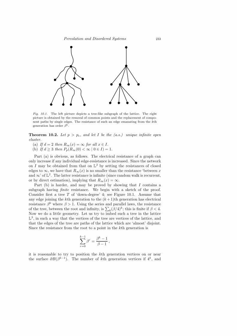
Percolation and Disordered Systems 233
Fig. 10.1. The left picture depicts a tree-like subgraph of the lattice. The rightpicture is obtained by the removal of common points and the replacement of compo-nent paths by single edges. The resistance of such an edge emanating from the kthgeneration has order βk.
Theorem 10.2. Let p > pc, and let I be the (a.s.) unique infinite opencluster.
(a) If d = 2 then R∞(x) = ∞ for all x ∈ I.(b) If d ≥ 3 then Pp(R∞(0) <∞ | 0 ∈ I) = 1.
Part (a) is obvious, as follows. The electrical resistance of a graph canonly increase if any individual edge-resistance is increased. Since the networkon I may be obtained from that on L2 by setting the resistances of closededges to ∞, we have that R∞(x) is no smaller than the resistance ‘between xand ∞’ of L2. The latter resistance is infinite (since random walk is recurrent,or by direct estimation), implying that R∞(x) = ∞.
Part (b) is harder, and may be proved by showing that I contains asubgraph having finite resistance. We begin with a sketch of the proof.Consider first a tree T of ‘down-degree’ 4; see Figure 10.1. Assume thatany edge joining the kth generation to the (k+ 1)th generation has electricalresistance βk where β > 1. Using the series and parallel laws, the resistanceof the tree, between the root and infinity, is
∑k(β/4)k; this is finite if β < 4.
Now we do a little geometry. Let us try to imbed such a tree in the latticeL3, in such a way that the vertices of the tree are vertices of the lattice, andthat the edges of the tree are paths of the lattice which are ‘almost’ disjoint.Since the resistance from the root to a point in the kth generation is
k−1∑
r=0
βr =βk − 1
β − 1,
it is reasonable to try to position the kth generation vertices on or nearthe surface ∂B(βk−1). The number of kth generation vertices if 4k, and
234 Geoffrey Grimmett
the volume of ∂B(βk−1) has order β(k−1)(d−1). The above construction cantherefore only succeed when 4k < β(k−1)(d−1) for all large k, which is to saythat β > 41/(d−1).
This crude picture suggests the necessary inequalities
(10.3) 41/(d−1) < β < 4,
which can be satisfied if and only if d ≥ 3.Assume now that d ≥ 3. Our target is to show that the infinite cluster I
contains sufficiently many disjoint paths to enable a comparison of its effectiveresistance with that of the tree in Figure 10.1, and with some value of βsatisfying (10.3). In presenting a full proof of this, we shall use the followingtwo percolation estimates, which are consequences of the results of Chapter7.
Lemma 10.4. Assume that p > pc.(a) There exists a strictly positive constant γ = γ(p) such that
(10.5) Pp(B(n) ↔ ∞
)≥ 1 − e−γn for all n.
(b) Let σ > 1, and let A(n, σ) be the event that there exist two vertices insideB(n) with the property that each is joined by an open path to ∂B(σn) butthat there is no open path of B(σn) joining these two vertices. There existsa strictly positive constant δ = δ(p) such that
(10.6) Pp(A(n, σ)
)≤ e−δn(σ−1) for all n.
We restrict ourselves here to the case d = 3; the general case d ≥ 3 issimilar. The surface of B(n) is the union of six faces, and we concentrate onthe face
F (n) = x ∈ Z3 : x1 = n, |x2|, |x3| ≤ n.
We write Bk = B(3k) and Fk = F (3k). On Fk, we distinguish 4k points,namely
xk(i, j) = (idk, jdk), −2k−1 < i, j ≤ 2k−1
where dk = ⌊(4/3)k⌋. The xk(i, j) are distributed on Fk in the manner of arectangular grid, and they form the ‘centres of attraction’ corresponding tothe kth generation of the tree discussed above.
With each xk(i, j) we associate four points on Fk+1, namely those in theset
Ik(i, j) = xk+1(r, s) : r = 2i− 1, 2i, s = 2j − 1, 2j.These four points are called children of xk(i, j). The centroid of Ik(i, j) isdenoted Ik(i, j). We shall attempt to construct open paths from points nearxk(i, j) to points near to each member of Ik(i, j), and this will be achievedwith high probability. In order to control the geometry of such paths, weshall build them within certain ‘tubes’ to be defined next.
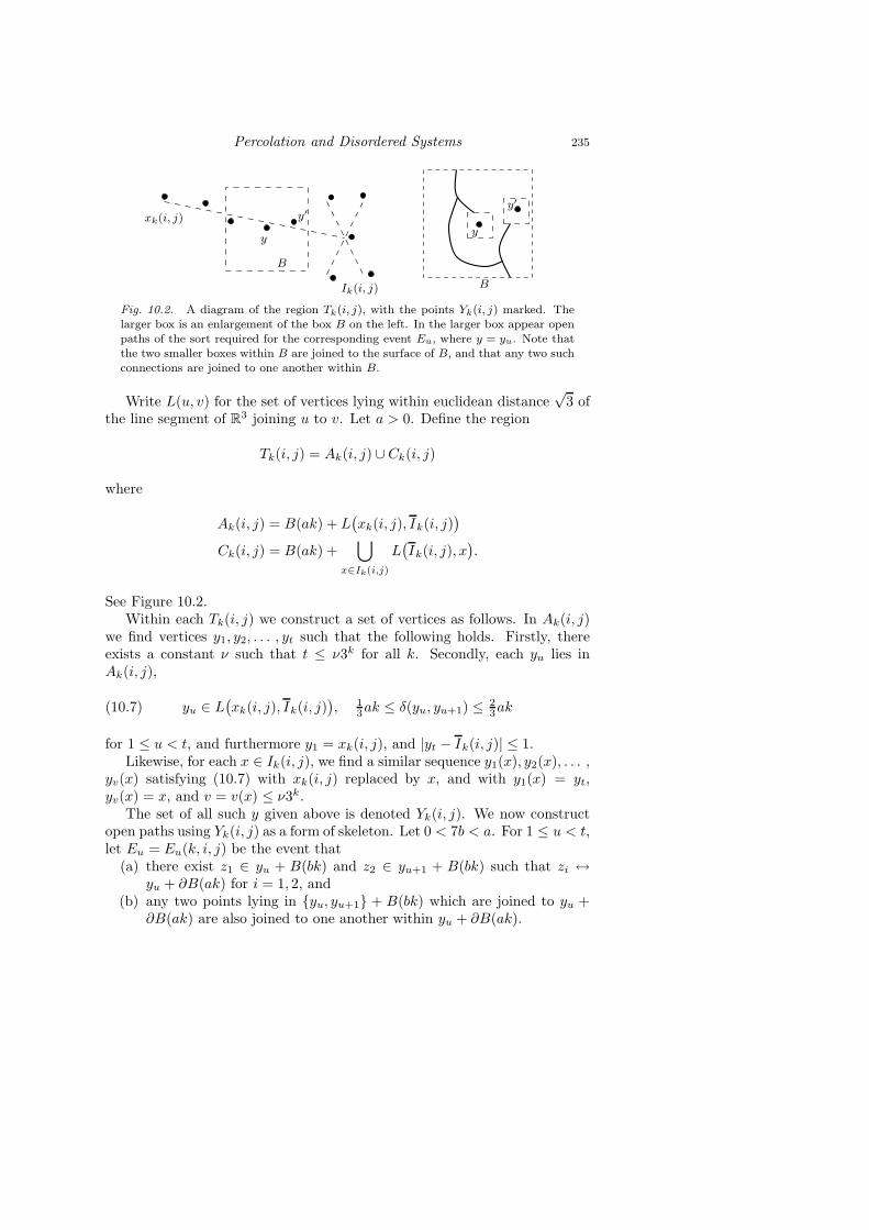
Percolation and Disordered Systems 235
xk(i, j)
yy
y′
y′
B
Ik(i, j) B
Fig. 10.2. A diagram of the region Tk(i, j), with the points Yk(i, j) marked. Thelarger box is an enlargement of the box B on the left. In the larger box appear openpaths of the sort required for the corresponding event Eu, where y = yu. Note thatthe two smaller boxes within B are joined to the surface of B, and that any two suchconnections are joined to one another within B.
Write L(u, v) for the set of vertices lying within euclidean distance√
3 ofthe line segment of R3 joining u to v. Let a > 0. Define the region
Tk(i, j) = Ak(i, j) ∪ Ck(i, j)
where
Ak(i, j) = B(ak) + L(xk(i, j), Ik(i, j)
)
Ck(i, j) = B(ak) +⋃
x∈Ik(i,j)
L(Ik(i, j), x
).
See Figure 10.2.Within each Tk(i, j) we construct a set of vertices as follows. In Ak(i, j)
we find vertices y1, y2, . . . , yt such that the following holds. Firstly, thereexists a constant ν such that t ≤ ν3k for all k. Secondly, each yu lies inAk(i, j),
(10.7) yu ∈ L(xk(i, j), Ik(i, j)
), 1
3ak ≤ δ(yu, yu+1) ≤ 23ak
for 1 ≤ u < t, and furthermore y1 = xk(i, j), and |yt − Ik(i, j)| ≤ 1.Likewise, for each x ∈ Ik(i, j), we find a similar sequence y1(x), y2(x), . . . ,
yv(x) satisfying (10.7) with xk(i, j) replaced by x, and with y1(x) = yt,yv(x) = x, and v = v(x) ≤ ν3k.
The set of all such y given above is denoted Yk(i, j). We now constructopen paths using Yk(i, j) as a form of skeleton. Let 0 < 7b < a. For 1 ≤ u < t,let Eu = Eu(k, i, j) be the event that
(a) there exist z1 ∈ yu + B(bk) and z2 ∈ yu+1 + B(bk) such that zi ↔yu + ∂B(ak) for i = 1, 2, and
(b) any two points lying in yu, yu+1 + B(bk) which are joined to yu +∂B(ak) are also joined to one another within yu + ∂B(ak).

236 Geoffrey Grimmett
We define similar events Ex,u = Ex,u(k, i, j) for x ∈ Ik(i, j) and 1 ≤ u < v =v(x), and finally let
Ek(i, j) =
⋂
1≤u<t
Eu
∩
⋂
1≤u<v(x)x∈Ik(i,j)
Ex,u
.
Let us estimate Pp(Ek(i, j)). Using Lemma 10.4, we have that
(10.8) Pp(Ek(i, j)) ≤ 5ν3ke−γbk + 5ν3ke−δak/6.
We call xm+l(r, s) a descendant of xm(0, 0) if it is a child of a child . . . of achild of xm(0, 0). Write Km for the set of all (m+ l, r, s) such that xm+l(r, s)is a descendant of xm(0, 0). We have from (10.8) that
Um =∑
(k,r,s)∈Km
Pp(Ek(r, s)) ≤∞∑
k=m
4k−m5ν3k(e−γbk + e−δak/6).
Now pick a, b such that 0 < 7b < a and e−γb, e−δa/6 < 112 , so that Um → 0 as
m → ∞. This implies that there exists a (random) value M of m such thatEk(r, s) occurs for all (k, r, s) ∈ KM .
Turning to the geometry implied in the definition of the Ek(r, s), we findthat the infinite open cluster contains a topological copy of the tree in Figure10.1, where the length of a path joining a kth generation vertex to one of itschildren is no greater than Ck33k for some constant C. In particular, thislength is smaller than C′βk for any β satisfying 3 < β < 4 and for someC′ = C′(β). Choosing β and C′ accordingly, and referring to the discussionaround (10.3), we conclude that I contains a tree having finite resistancebetween its root and infinity. The second claim of Theorem 10.2 follows.
10.2 Random Walks in Two-Dimensional Labyrinths
A beautiful question dating back to Lorentz [246] and Ehrenfest [128] con-cerns the behaviour of a particle moving in Rd but scattered according toreflecting obstacles distributed about Rd. There is a notorious lattice versionof this question which is largely unsolved. Start with the two-dimensionalsquare lattice L2. A reflector may be placed at any vertex in either of twoways: either it is a NW reflector (which deflects incoming rays heading north-wards, resp. southwards, to the west, resp. east, and vice versa) or it is a NEreflector (defined similarly); see Figure 10.3. Think of a reflector as beinga two-sided mirror placed at 45 to the axes, so that an incoming light rayis reflected along an axis perpendicular to its direction of arrival. Now, foreach vertex x, with probability p we place a reflector at x, and otherwise we

Percolation and Disordered Systems 237
NW NE
Fig. 10.3. NW and NE reflectors in action.
Fig. 10.4. (a) The heavy lines form the lattice L2A, and the central point is the origin
of L2. (b) An open circuit in L
2A constitutes a barrier of mirrors through which no
light may penetrate.
place nothing at x. This is done independently for different x. If a reflectoris placed at x, then we specify that it is equally likely to be NW as NE.
We shine a torch northwards from the origin. The light is reflected bythe mirrors, and we ask whether or not the light ray returns to the origin.Letting
η(p) = Pp(the light ray returns to the origin),
we would like to know for which values of p it is the case that η(p) = 1. Itis reasonable to conjecture that η is non-decreasing in p. Certainly η(0) = 0,and it is ‘well known’ that η(1) = 1.
Theorem 10.9. It is the case the η(1) = 1.
Proof of Theorem 10.9. This proof is alluded to in [G] and included in [81].From L2 we construct an ancillary lattice L2
A as follows. Let
A =
(m+ 12 , n+ 1
2 ) : m+ n is even.
On A we define the adjacency relation ∼ by (m+ 12 , n+ 1
2 ) ∼ (r + 12 , s+ 1
2 )
if and only if |m− r| = |n− s| = 1, obtaining thereby a copy of L2 denoted
as L2A. See Figure 10.4.
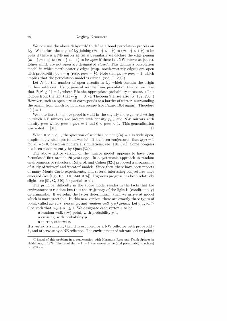
238 Geoffrey Grimmett
We now use the above ‘labyrinth’ to define a bond percolation process onL2A. We declare the edge of L2
A joining (m− 12 , n− 1
2 ) to (m+ 12 , n+ 1
2 ) to beopen if there is a NE mirror at (m,n); similarly we declare the edge joining(m− 1
2 , n+ 12 ) to (m+ 1
2 , n− 12 ) to be open if there is a NW mirror at (m,n).
Edges which are not open are designated closed . This defines a percolationmodel in which north-easterly edges (resp. north-westerly edges) are openwith probability pNE = 1
2 (resp. pNW = 12 ). Note that pNE + pNW = 1, which
implies that the percolation model is critical (see [G, 203]).Let N be the number of open circuits in L2
A which contain the originin their interiors. Using general results from percolation theory, we havethat P(N ≥ 1) = 1, where P is the appropriate probability measure. (Thisfollows from the fact that θ(1
2 ) = 0; cf. Theorem 9.1, see also [G, 182, 203].)However, such an open circuit corresponds to a barrier of mirrors surroundingthe origin, from which no light can escape (see Figure 10.4 again). Thereforeη(1) = 1.
We note that the above proof is valid in the slightly more general settingin which NE mirrors are present with density pNE and NW mirrors withdensity pNW where pNW + pNE = 1 and 0 < pNW < 1. This generalisationwas noted in [81].
When 0 < p < 1, the question of whether or not η(p) = 1 is wide open,despite many attempts to answer it7. It has been conjectured that η(p) = 1for all p > 0, based on numerical simulations; see [110, 375]. Some progresshas been made recently by Quas [320].
The above lattice version of the ‘mirror model’ appears to have beenformulated first around 20 years ago. In a systematic approach to randomenvironments of reflectors, Ruijgrok and Cohen [324] proposed a programmeof study of ‘mirror’ and ‘rotator’ models. Since then, there have been reportsof many Monte Carlo experiments, and several interesting conjectures haveemerged (see [108, 109, 110, 343, 375]). Rigorous progress has been relativelyslight; see [81, G, 320] for partial results.
The principal difficulty in the above model resides in the facts that theenvironment is random but that the trajectory of the light is (conditionally)deterministic. If we relax the latter determinism, then we arrive at modelwhich is more tractable. In this new version, there are exactly three types ofpoint, called mirrors, crossings, and random walk (rw) points . Let prw, p+ ≥0 be such that prw + p+ ≤ 1. We designate each vertex x to be
a random walk (rw) point, with probability prw,a crossing, with probability p+,a mirror, otherwise.
If a vertex is a mirror, then it is occupied by a NW reflector with probability12 , and otherwise by a NE reflector. The environment of mirrors and rw points
7I heard of this problem in a conversation with Hermann Rost and Frank Spitzer inHeidelberg in 1978. The proof that η(1) = 1 was known to me (and presumably to others)in 1978 also.
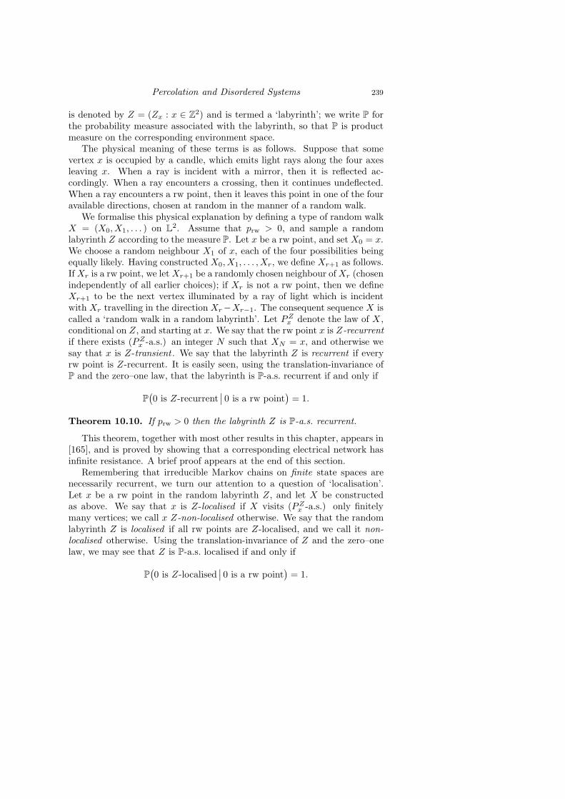
Percolation and Disordered Systems 239
is denoted by Z = (Zx : x ∈ Z2) and is termed a ‘labyrinth’; we write P forthe probability measure associated with the labyrinth, so that P is productmeasure on the corresponding environment space.
The physical meaning of these terms is as follows. Suppose that somevertex x is occupied by a candle, which emits light rays along the four axesleaving x. When a ray is incident with a mirror, then it is reflected ac-cordingly. When a ray encounters a crossing, then it continues undeflected.When a ray encounters a rw point, then it leaves this point in one of the fouravailable directions, chosen at random in the manner of a random walk.
We formalise this physical explanation by defining a type of random walkX = (X0, X1, . . . ) on L
2. Assume that prw > 0, and sample a randomlabyrinth Z according to the measure P. Let x be a rw point, and set X0 = x.We choose a random neighbour X1 of x, each of the four possibilities beingequally likely. Having constructed X0, X1, . . . , Xr, we define Xr+1 as follows.If Xr is a rw point, we let Xr+1 be a randomly chosen neighbour ofXr (chosenindependently of all earlier choices); if Xr is not a rw point, then we defineXr+1 to be the next vertex illuminated by a ray of light which is incidentwith Xr travelling in the direction Xr−Xr−1. The consequent sequence X iscalled a ‘random walk in a random labyrinth’. Let PZx denote the law of X ,conditional on Z, and starting at x. We say that the rw point x is Z-recurrentif there exists (PZx -a.s.) an integer N such that XN = x, and otherwise wesay that x is Z-transient . We say that the labyrinth Z is recurrent if everyrw point is Z-recurrent. It is easily seen, using the translation-invariance ofP and the zero–one law, that the labyrinth is P-a.s. recurrent if and only if
P(0 is Z-recurrent
∣∣ 0 is a rw point)
= 1.
Theorem 10.10. If prw > 0 then the labyrinth Z is P-a.s. recurrent.
This theorem, together with most other results in this chapter, appears in[165], and is proved by showing that a corresponding electrical network hasinfinite resistance. A brief proof appears at the end of this section.
Remembering that irreducible Markov chains on finite state spaces arenecessarily recurrent, we turn our attention to a question of ‘localisation’.Let x be a rw point in the random labyrinth Z, and let X be constructedas above. We say that x is Z-localised if X visits (PZx -a.s.) only finitelymany vertices; we call x Z-non-localised otherwise. We say that the randomlabyrinth Z is localised if all rw points are Z-localised, and we call it non-localised otherwise. Using the translation-invariance of Z and the zero–onelaw, we may see that Z is P-a.s. localised if and only if
P(0 is Z-localised
∣∣ 0 is a rw point)
= 1.

240 Geoffrey Grimmett
p+
1
prwpc(site)1
Fig. 10.5. The grey region and the heavy lines of the figure indicate the part of(prw, p+) space for which non-localisation is proved. The labyrinth is a.s. localisedwhen prw = p+ = 0; see Theorem 10.9.
Theorem 10.11. Let prw > 0. There exists a strictly positive constantA = A(prw) such that the following holds. The labyrinth Z is P-a.s. non-localised if any of the following conditions hold:
(a) prw > pc(site), the critical probability of site percolation on L2,(b) p+ = 0,(c) prw + p+ > 1 −A.
We shall see in the proof of part (c) (see Theorem 10.17) that A(prw) → 0as prw ↓ 0. This fact is reported in Figure 10.5, thereby correcting an errorin the corresponding figure contained in [165].
Proof of Theorem 10.10. Assume prw > 0. We shall compare the labyrinthwith a certain electrical network. By showing that the effective resistanceof this network between 0 and ∞ is a.s. infinite, we shall deduce that Z isa.s. recurrent. For details of the relationship between Markov chains andelectrical networks, see the book [117] and the papers [252, 276].
By the term Z-path we mean a path of the lattice (possibly with self-intersections) which may be followed by the light; i.e., at rw points it isunconstrained, while at reflectors and crossings it conforms to the appropriaterule. A formal definition will be presented in Section 10.3.
Let e = 〈u, v〉 be an edge of L2. We call e a normal edge if it lies insome Z-path π(e) which is minimal with respect to the property that its twoendvertices (and no others) are rw points, and furthermore that these twoendvertices are distinct. If e is normal, we write l(e) for the number of edgesin π(e); if e is not normal, we write l(e) = 0. We define ρ(e) = 1/l(e), withthe convention that 1/0 = ∞.

Percolation and Disordered Systems 241
Next, we construct an electrical network E(ρ) on L2 by, for each edgee of L2, placing an electrical resistor of size ρ(e) at e. Let R = R(Z) bethe effective resistance of this network between 0 and ∞ (which is to saythat R = limn→∞Rn, where Rn is the resistance between 0 and a compositevertex obtained by identifying all vertices in ∂B(n)).
Lemma 10.12. We have that P(R(Z) = ∞
∣∣ 0 is a rw point)
= 1.
Proof. We define the ‘edge-boundary’ ∆eB(n) of B(n) to be the set of edgese = 〈x, y〉 with x ∈ ∂B(n) and y ∈ ∂B(n+ 1). We claim that there exists apositive constant c and a random integer M such that
(10.13) ρ(e) ≥ c
lognfor all e ∈ ∆eB(n) and n ≥M.
To show this, we argue as follows. Assume that e = 〈x, y〉 is normal, and letλ1 be the number of edges in the path π(e) on one side of e (this side beingchosen in an arbitrary way), and λ2 for the number on the other side. Sinceeach new vertex visited by the path is a rw point with probability prw, andsince no vertex appears more than twice in π(e), we have that
P(l(e) > 2k, e is normal
)≤ 2P
(λ1 ≥ k, e is normal
)≤ 2(1 − prw)
12 (k−1).
Therefore, for c > 0 and all n ≥ 2,
P
(ρ(e) <
c
log nfor some e ∈ ∆eB(n)
)
≤ 4(2n+ 1)P
(l(e) >
logn
c, e is normal
)
≤ βn1−α
where α = α(c) = −(4c)−1 log(1 − prw) and β = β(c, prw) <∞. We choose csuch that α > 5
2 , whence (10.13) follows by the Borel–Cantelli lemma.The conclusion of the lemma is a fairly immediate consequence of (10.13),
using the usual argument which follows. From the electrical network E(ρ)we construct another network with no larger resistance. This we do by iden-tifying all vertices contained in each ∂B(n). In this new system there are|∆eB(n)| parallel connections between ∂B(n) and ∂B(n+ 1), each of whichhas (for n ≥ M) a resistance at least c/ logn. The effective resistance fromthe origin to infinity is therefore at least
∞∑
n=M
c
|∆eB(n)| logn=
∞∑
n=M
c
4(2n+ 1) logn= ∞,
and the proof of the lemma is complete.
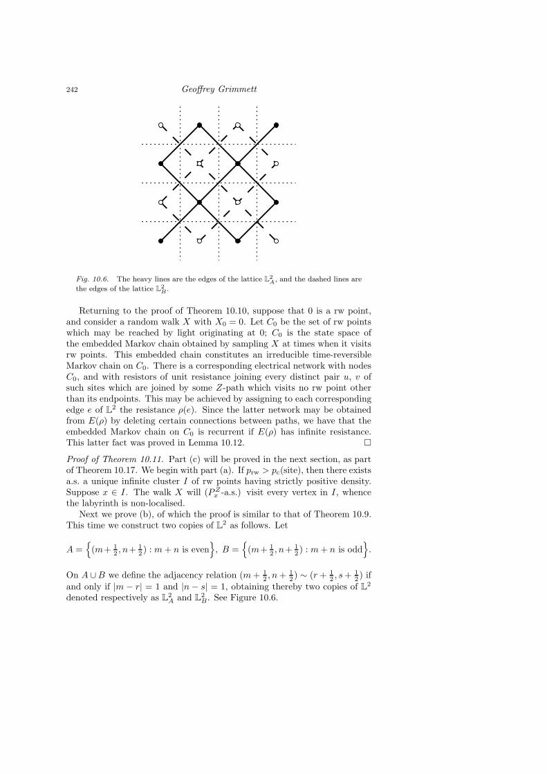
242 Geoffrey Grimmett
Fig. 10.6. The heavy lines are the edges of the lattice L2A, and the dashed lines are
the edges of the lattice L2B .
Returning to the proof of Theorem 10.10, suppose that 0 is a rw point,and consider a random walk X with X0 = 0. Let C0 be the set of rw pointswhich may be reached by light originating at 0; C0 is the state space ofthe embedded Markov chain obtained by sampling X at times when it visitsrw points. This embedded chain constitutes an irreducible time-reversibleMarkov chain on C0. There is a corresponding electrical network with nodesC0, and with resistors of unit resistance joining every distinct pair u, v ofsuch sites which are joined by some Z-path which visits no rw point otherthan its endpoints. This may be achieved by assigning to each correspondingedge e of L
2 the resistance ρ(e). Since the latter network may be obtainedfrom E(ρ) by deleting certain connections between paths, we have that theembedded Markov chain on C0 is recurrent if E(ρ) has infinite resistance.This latter fact was proved in Lemma 10.12.
Proof of Theorem 10.11. Part (c) will be proved in the next section, as partof Theorem 10.17. We begin with part (a). If prw > pc(site), then there existsa.s. a unique infinite cluster I of rw points having strictly positive density.Suppose x ∈ I. The walk X will (PZx -a.s.) visit every vertex in I, whencethe labyrinth is non-localised.
Next we prove (b), of which the proof is similar to that of Theorem 10.9.This time we construct two copies of L
2 as follows. Let
A =
(m+ 12 , n+ 1
2 ) : m+ n is even, B =
(m+ 1
2 , n+ 12 ) : m+ n is odd
.
On A ∪B we define the adjacency relation (m+ 12 , n+ 1
2 ) ∼ (r+ 12 , s+ 1
2 ) if
and only if |m − r| = 1 and |n− s| = 1, obtaining thereby two copies of L2
denoted respectively as L2A and L2
B. See Figure 10.6.
Percolation and Disordered Systems 243
We now define bond percolation processes on L2A and L2
B . Assume p+ = 0.We present the rules for L2
A only; the rules for L2B are analogous. An edge of
L2A joining (m− 1
2 , n− 12 ) to (m+ 1
2 , n+ 12 ) to declared to be open if there is
a NE mirror at (m,n); similarly we declare the edge joining (m − 12 , n + 1
2 )
to (m+ 12 , n− 1
2 ) to be open if there is a NW mirror at (m,n). Edges which
are not open are called closed . This defines percolation models on L2A and
L2B in which north-easterly edges (resp. north-westerly edges) are open with
probability pNE = 12 (1 − prw) (resp. pNW = 1
2 (1 − prw)). These processes aresubcritical since pNE + pNW = 1 − prw < 1. Therefore, there exists (P-a.s.)no infinite open path in either L2
A or L2B , and we assume henceforth that no
such infinite open path exists.Let N(A) (resp. N(B)) be the number of open circuits in L2
A (resp. L2B)
which contain the origin in their interiors. Since the above percolation pro-cesses are subcritical, there exists (by Theorem 6.10) a strictly positive con-stant α = α(pNW, pNE) such that(10.14)
P
(x lies in an open cluster of L
2A of diameter at least n
)≤ e−αn for all n,
for any vertex x of L2A. (By the diameter of a set C of vertices, we mean
max|y− z| : y, z ∈ C.) The same conclusion is valid for L2B. We claim that
(10.15) P(0 is a rw point, and N(A) = N(B) = 0
)> 0,
and we prove this as follows. Let Λ(k) = [−k, k]2, and let Nk(A) (resp.Nk(B)) be the number of circuits contributing to N(A) (resp. N(B)) whichcontain only points lying strictly outside Λ(k). If Nk(A) ≥ 1 then there existssome vertex (m+ 1
2 ,12 ) of L2
A, with m ≥ k, which belongs to an open circuitof diameter exceeding m. Using (10.14),
P(Nk(A) ≥ 1
)≤
∞∑
m=k
e−αm < 13
for sufficiently large k. We pick k accordingly, whence
P(Nk(A) +Nk(B) ≥ 1
)≤ 2
3 .
Now, if Nk(A) = Nk(B) = 0, and in addition all points of L2 inside Λ(k) arerw points, then N(A) = N(B) = 0. These last events have strictly positiveprobabilities, and (10.15) follows.
Let J be the event that there exists a rw point x = x(Z) which lies inthe interior of no open circuit of either L2
A or L2B . Since J is invariant with
respect to translations of L2, and since P is product measure, we have thatP(J) equals either 0 or 1. Using (10.15), we deduce that P(J) = 1. Thereforewe may find a.s. some such vertex x = x(Z). We claim that x is Z-non-localised, which will imply as claimed that the labyrinth if a.s. non-localised.

244 Geoffrey Grimmett
Fig. 10.7. The solid line in each picture is the edge e = 〈u, v〉, and the central vertexis u. If all three of the other edges of L2
A incident with the vertex u are closed in L2A,
then there are eight possibilities for the corresponding edges of L2B . The dashed lines
indicate open edges of L2B , and the crosses mark rw points of L
2. In every picture,light incident with one side of the mirror at e will illuminate the other side also.
Let Cx be the set of rw points reachable by light originating at the rwpoint x. The set Cx may be generated in the following way. We allow lightto leave x along the four axial directions. When a light ray hits a crossing ora mirror, it follows the associated rule; when a ray hits a rw point, it causeslight to depart the point along each of the other three axial directions. NowCx is the set of rw points thus reached. Following this physical picture, letF be the set of ‘frontier mirrors’, i.e., the set of mirrors only one side ofwhich is illuminated. Assume that F is non-empty, say F contains a mirrorat some point (m,n). Now this mirror must correspond to an open edge ein either L2
A and L2B (see Figure 10.6 again), and we may assume without
loss of generality that this open edge e is in L2A. We write e = 〈u, v〉 where
u, v ∈ A, and we assume that v = u + (1, 1); an exactly similar argumentholds otherwise. There are exactly three other edges of L2
A which are incidentto u (resp. v), and we claim that one of these is open. To see this, argue asfollows. If none is open, then
u+ (− 12 ,
12 ) either is a rw point or has a NE mirror,
u+ (− 12 ,− 1
2 ) either is a rw point or has a NW mirror,
u+ (12 ,− 1
2 ) either is a rw point or has a NE mirror.See Figure 10.7 for a diagram of the eight possible combinations. By inspec-tion, each such combination contradicts the fact that e = 〈u, v〉 correspondsto a frontier mirror.
Therefore, u is incident to some other open edge f of L2A, other than e.
By a further consideration of each of 23−1 possibilities, we may deduce thatthere exists such an edge f lying in F . Iterating the argument, we find that elies in either an open circuit or an infinite open path of F lying in L2
A. Since

Percolation and Disordered Systems 245
there exists (by assumption) no infinite open path, this proves that f lies inan open circuit of F in L2
A.By taking the union over all e ∈ F , we obtain that F is a union of open
circuits of L2A and L2
B . Each such circuit has an interior and an exterior, andx lies (by assumption, above) in every exterior. There are various ways ofdeducing that x is Z-non-localised, and here is such a way.
Assume that x is Z-localised. Amongst the set of vertices x + (n, 0) :n ≥ 1, let y be the rightmost vertex at which there lies a frontier mirror.By the above argument, y belongs to some open circuit G of F (belonging toeither L2
A or L2B), whose exterior contains x. Since y is rightmost, we have
that y′ = y + (−1, 0) is illuminated by light originating at x, and that lighttraverses the edge 〈y′, y〉. Similarly, light does not traverse the edge 〈y, y′′〉,where y′′ = y+ (1, 0). Therefore, the point y+ (1
2 , 0) of R2 lies in the interiorof G, which contradicts the fact that y is rightmost. This completes the prooffor part (b).
10.3 General Labyrinths
There are many possible types of reflector, especially in three and more di-mensions. Consider Zd where d ≥ 2. Let I = u1, u2, . . . , ud be the set ofpositive unit vectors, and let I± = −1,+1× I; members of I± are writtenas ±uj. We make the following definition. A reflector is a map ρ : I± → I±
satisfying ρ(−ρ(u)) = −u for all u ∈ I±. We denote by R the set of reflectors.The ‘identity reflector’ is called a crossing (this is the identity map on I±),and denoted by +.
The physical interpretation of a reflector is as follows. If light impingeson a reflector ρ, moving in a direction u (∈ I±) then it is required to departthe reflector in the direction ρ(u). The condition ρ(−ρ(u)) = −u arises fromthe reversibility of reflections.
Using elementary combinatorics, one may calculate that the number ofdistinct reflectors in d dimensions is
d∑
s=0
(2d)!
(2s)! 2d−s(d− s)!.
A random labyrinth is constructed as follows. Let prw and p+ be non-negative reals satisfying prw +p+ ≤ 1. Let Z = (Zx : x ∈ Zd) be independentrandom variables taking values in R∪ ∅, with common mass function
P(Z0 = α) =
prw if α = ∅
p+ if α = +
(1 − prw − p+)π(ρ) if α = ρ ∈ R\+,
where π is a prescribed probability mass function on R\+. We call a pointx a crossing if Zx = +, and a random walk (rw) point if Zx = ∅.

246 Geoffrey Grimmett
A Ld-path is defined to be a sequence x0, e0, x1, e1, . . . of alternating ver-tices xi and distinct edges ej such that ej = 〈xj , xj+1〉 for all j. If the pathhas a final vertex xn, then it is said to have length n and to join x0 to xn.If it is infinite, then it is said to join x0 to ∞. A Ld-path may visit verticesmore than once, but we insist that its edges be distinct.
We define a Z-path to be a Ld-path x0, e0, x1, e1, . . . with the propertythat, for all j,
xj+1 − xj = Zxj(xj − xj−1) whenever Zxj
6= ∅,
which is to say that the path conforms to all reflectors.Let N be the set of rw points. We define an equivalence relation ↔ on N
by x ↔ y if and only if there exists a Z-path with endpoints x and y. Wedenote by Cx the equivalence class of (N,↔) containing the rw point x, andby C the set of equivalence classes of (N,↔). The following lemma will beuseful; a sketch proof is deferred to the end of the section.
Lemma 10.16. Let d ≥ 2 and prw > 0. The number M of equivalenceclasses of (N,↔) having infinite cardinality satisfies
either P(M = 0) = 1 or P(M = 1) = 1.
Next we define a random walk in the random labyrinth Z. Let x be a rwpoint. A walker, starting at x, flips a fair coin (in the manner of a symmetricrandom walker) whenever it arrives at a rw point in order to determine itsnext move. When it meets a reflector, it moves according to the reflector (i.e.,if it strikes the reflector ρ in the direction u, then it departs in the directionρ(u)). Writing PZx for the law of the walk, we say that the point x is Z-recurrent if PZx (XN = x for some N ≥ 1) = 1, and Z-transient otherwise.As before, we say that Z is transient if there exists a rw point x which isZ-transient, and recurrent otherwise.
Note that, if the random walker starts at the rw point x, then the se-quence of rw points visited constitutes an irreducible Markov chain on theequivalence class Cx. Therefore, the rw point x is Z-localised if and only if|Cx| <∞. As before, we say that Z is localised if all rw points are Z-localised,and non-localised otherwise.
Theorem 10.17. Let prw > 0. There exists a strictly positive constantA = A(prw, d) such that the following holds.
(a) Assume that d ≥ 2. If 1− prw − p+ < A, then the labyrinth Z is P-a.s.non-localised.
(b) Assume that d ≥ 3. If 1 − prw − p+ < A, then Z is P-a.s. transient.
As observed after 10.11, we have that A = A(prw, d) → 0 as prw ↓ 0.Using methods presented in [114, 115, 220], one may obtain an invariance
principle for a random walk in a random labyrinth, under the condition that1 − prw − p+ is sufficiently small. Such a principle is valid for a walk which

Percolation and Disordered Systems 247
starts in the (a.s) unique infinite equivalence class of Z. The details willappear in [73].
The following proof of Theorem 10.17 differs from that presented in [165]8.It is slightly more complicated, but gives possibly a better numerical valuefor the constant A.
Proof. The idea is to relate the labyrinth to a certain percolation process,as follows. We begin with the usual lattice Ld = (Zd,Ed), and from this weconstruct the ‘line lattice’ (or ‘covering lattice’) L as follows. The vertex setof L is the edge-set Ed of Ld, and two distinct vertices e1, e2 (∈ Ed) of L arecalled adjacent in L if and only if they have a common vertex of Ld. If thisholds, we write 〈e1, e2〉 for the corresponding edge of L, and denote by F theset of all such edges. We shall work with the graph L = (Ed,F), and shallconstruct a bond percolation process on L. We may identify Ed with the setof midpoints of members of E; this embedding is useful in visualising L.
Let 〈e1, e2〉 ∈ Ed. If the edges e1 and e2 of Ld are perpendicular, wecolour 〈e1, e2〉 amber , and if they are parallel blue. Let 0 ≤ α, β ≤ 1. Wedeclare an edge 〈e1, e2〉 of F to be open with probability α (if amber) or β(if blue). This we do for each 〈e, f〉 ∈ F independently of all other membersof F. Write Pα,β for the corresponding probability measure, and let θ(α, β)be the probability that a given vertex e (∈ Ed) of L is in an infinite opencluster of the ensuing percolation process on L. It is easily seen that θ(α, β)is independent of the choice of e.
Lemma 10.18. Let d ≥ 2 and 0 < α ≤ 1. then
βc(α, d) = supβ : θ(α, β) = 0
satisfies βc(α, d) < 1.
Note that, when d = 2 and β = 0, the process is isomorphic to bond per-colation on L2 with edge-parameter α. Therefore θ(α, 0) > 0 and βc(α, 2) = 0when α > 1
2 .
Proof. Since βc(α, d) is non-increasing in d, it suffices to prove the conclusionwhen d = 2. Henceforth assume that d = 2.
Here is a sketch proof. Let L ≥ 1 and let AL be the event that everyvertex of L lying within the box B(L + 1
2 ) = [−L − 12 , L + 1
2 ]2 (of R2) is
joined to every other vertex lying within B(L+ 12 ) by open paths of L lying
inside B(L + 12 ) which do not use boundary edges. For a given α satisfying
0 < α < 1, there exist L and β′ such that
Pα,β′(AL) ≥ pc(site),
8There is a small error in the proof of Theorem 7 of [165], but this may easily becorrected.
248 Geoffrey Grimmett
where pc(site) is the critical probability of site percolation on L2. Now tileZ2 with copies of B(L + 1
2 ), overlapping at the sides. It follows from theobvious relationship with site percolation that, with positive probability, theorigin lies in an infinite cluster.
We now construct a labyrinth on Zd from each realisation ω ∈ 0, 1F ofthe percolation process (where we write ω(f) = 1 if and only if the edge fis open). That is, with each point x ∈ Zd we shall associate a member ρxof R ∪ ∅, in such a way that ρx depends only on the edges 〈e1, e2〉 of F
for which e1 and e2 are distinct edges of Ld having common vertex x. Itwill follow that the collection ρx : x ∈ Zd is a family of independent andidentically distributed objects.
Since we shall define the ρx according to a translation-invariant rule, it willsuffice to present only the definition of the reflector ρ0 at the origin. Let E0 bethe set of edges of Ld which are incident to the origin. There is a natural one–one correspondence between E0 and I±, namely, the edge 〈0, u〉 correspondsto the unit vector u ∈ I±. Let ρ ∈ R. Using the above correspondence, wemay associate with ρ a set of configurations in Ω = 0, 1F, as follows. LetΩ(ρ, 0) be the subset of Ω containing all configurations ω satisfying
ω(〈0, u1〉, 〈0, u2〉
)= 1 if and only if ρ(−u1) = u2
for all distinct pairs u1, u2 ∈ I±.It is not difficult to see that
Ω(ρ1, 0) ∩ Ω(ρ2, 0) = ∅ if ρ1, ρ2 ∈ R, ρ1 6= ρ2.
Let ω ∈ Ω be a percolation configuration on F. We define the reflectorρ0 = ρ0(ω) at the origin by
(10.19) ρ0 =
ρ if ω ∈ Ω(ρ, 0)
∅ if ω /∈ ⋃ρ∈R Ω(ρ, 0).
If ρ0 = ρ ∈ R, then the behaviour of a light beam striking the originbehaves as in the corresponding percolation picture, in the following sense.Suppose light is incident in the direction u1. There exists at most one direc-tion u2 (6= u1) such that ω(〈0,−u1〉, 〈0, u2〉) = 1. If such a u2 exists, thenthe light is reflected in this direction. If no such u2 exists, then it is reflectedback on itself, i.e., in the direction −u1.
For ω ∈ 0, 1F, the above construction results in a random labyrinthL(ω). If the percolation process contains an infinite open cluster, then thecorresponding labyrinth contains (a.s.) an infinite equivalence class.
Turning to probabilities, it is easy to see that, for ρ ∈ R,
π(ρ;α, β) = Pα,β(ρ0 = ρ)

Percolation and Disordered Systems 249
satisfies π(ρ;α, β) > 0 if 0 < α, β < 1, and furthermore
π(+;α, β) = βd(1 − α)(2d
2 )−d.
Also,
π(∅;α, β) = Pα,β(ρ0 = ∅) = 1 −∑
ρ∈R
π(ρ;α, β).
Let prw, p+ satisfy prw, p+ > 0, prw + p+ ≤ 1. We pick α, β such that0 < α, β < 1, β > βc(α, 2) and
(10.20) π(+;α, β) ≥ 1 − prw (≥ p+).
(That this may be done is a consequence of the fact that βc(α, 2) < 1 for allα > 0; cf. Lemma 10.18.)
With this choice of α, β, let
A = min
π(ρ;α, β)
π(ρ): ρ 6= +, ρ ∈ R
with the convention that 1/0 = ∞. (Thus defined, A depends on π as well ason prw. If we set A = min
π(ρ;α, β) : ρ 6= +, ρ ∈ R
, we obtain a (smaller)
constant which is independent of π, and we may work with this definitioninstead.) Then
π(ρ;α, β) ≥ Aπ(ρ) for all ρ 6= +,
and in particular
(10.21) π(ρ;α, β) ≥ (1 − prw − p+)π(ρ) if ρ 6= +
so long as p+ satisfies 1 − prw − p+ < A. Note that A = A(α, β) > 0.We have from the fact that β > βc(α, 2) that the percolation process ω
a.s. contains an infinite open cluster. It follows that there exists a.s. a rwpoint in L(ω) which is L(ω)-non-localised. The labyrinth Z of the theoremmay be obtained (in distribution) from L as follows. Having sampled L(ω),we replace any crossing (resp. reflector ρ (6= +)) by a rw point with proba-bility π(+;α, β) − p+ (resp. π(ρ;α, β) − (1 − prw − p+)π(ρ)); cf. (10.20) and(10.21). The ensuing labyrinth L′(ω) has the same probability distributionas Z. Furthermore, if L(ω) is non-localised, then so is L′(ω).
The first part of Theorem 10.17 has therefore been proved. Assume hence-forth that d ≥ 3, and consider part (b).
Now consider a labyrinth defined by prw, p+, π(·). Let e be an edge of Zd.Either e lies in a unique path joining two rw points (but no other rw point)of some length l(e), or it does not (in which case we set l(e) = 0). Now,the random walk in this labyrinth induces an embedded Markov chain on theset of rw points. This chain corresponds to an electrical network obtainedby placing an electrical resistor at each edge e having resistance l(e)−1. We

250 Geoffrey Grimmett
now make two comparisons, the effect of each of which is to increase alleffective resistances of the network. At the first stage, we replace all finiteedge-resistances l(e)−1 by unit resistances. This cannot decrease any effectiveresistance. At the next stage we replace each rw point by
+ with probability π(+;α, β) − p+
ρ (6= +) with probability π(ρ;α, β) − (1 − prw − p+)π(ρ),
in accordance with (10.20) and (10.21) (and where α, β are chosen so that(10.20), (10.21) hold, and furthermore βc(α, 2) < β < 1). Such replacementscan only increase effective resistance.
In this way we obtain a comparison between the resistance of the net-work arising from the above labyrinth and that of the labyrinth L(ω) definedaround (10.19). Indeed, it suffices to prove that the effective resistance be-tween 0 and ∞ (in the infinite equivalence class) of the labyrinth L(ω) is a.s.finite. By examining the geometry, we claim that this resistance is no greater(up to a multiplicative constant) than the resistance between the origin andinfinity of the corresponding infinite open percolation cluster of ω. By thenext lemma, the last resistance is a.s. finite, whence the original walk isa.s. transient (when confined to the almost surely unique infinite equivalenceclass).
Lemma 10.22. Let d ≥ 3, 0 < α < 1, and βc(α, 2) < β < 1. Let R be theeffective resistance between the origin and the points at infinity, in the abovebond percolation process ω on L. Then
Pα,β(R <∞
∣∣ 0 belongs to the infinite open cluster)
= 1.
Presumably the same conclusion is valid under the weaker hypothesis thatβ > βc(α, d).
Sketch Proof. Rather than present all the details, here are some notes. Themain techniques used in [163] arise from [164], and principally one uses theexponential decay noted in Lemma 10.4. That such decay is valid wheneverβ > βc(α, d) uses the machinery of [164]. This machinery may be developed inthe present setting (in [164] it is developed only for the hypercubic lattice Ld).Alternatively, ‘slab arguments’ show (a) and (b) of Lemma 10.4 for sufficientlylarge β; certainly the condition β > βc(α, 2) suffices for the conclusion.
Comments on the Proof of Lemma 10.16. This resembles closely the proofof the uniqueness of the infinite percolation cluster (Theorem 7.1). We donot give the details. The notion of ‘trifurcation’ is replaced by that of an‘encounter zone’. Let R ≥ 1 and B = B(R). A translate x + B is called anencounter zone if
(a) all points in x+B are rw points, and(b) in the labyrinth Zd\x+B, there are three or more infinite equivalence
classes which are part of the same equivalence class of Ld.
Note that different encounter zones may overlap. See [73] for details.

Percolation and Disordered Systems 251
11. FRACTAL PERCOLATION
11.1. Random Fractals
Many so called ‘fractals’ are generated by iterative schemes, of which theclassical middle-third Cantor construction is a canonical example. When thescheme incorporates a randomised step, then the ensuing set may be termeda ‘random fractal’. Such sets may be studied in some generality (see [130,152, 184, 312]), and properties of fractal dimension may be established. Thefollowing simple example is directed at a ‘percolative’ property, namely thepossible existence in the random fractal of long paths.
We begin with the unit square C0 = [0, 1]2. At the first stage, we divide C0
into nine (topologically closed) subsquares of side-length 13 (in the natural
way), and we declare each of the subsquares to be open with probabilityp (independently of any other subsquare). Write C1 for the union of theopen subsquares thus obtained. We now iterate this construction on eachsubsquare in C1, obtaining a collection of open (sub)subsquares of side-length19 . After k steps we have obtained a union Ck of open squares of side-length
(13 )k. The limit set
(11.1) C = limk→∞
Ck =⋂
k≥1
Ck
is a random set whose metrical properties we wish to study. See Figure 11.1.Constructions of the above type were introduced by Mandelbrot [255] and
initially studied by Chayes, Chayes, and Durrett [91]. Recent papers include[113, 133, 301]. Many generalisations of the above present themselves.
(a) Instead of working to base 3, we may work to base M where M ≥ 2.(b) Replace two dimensions by d dimensions where d ≥ 2.(c) Generalise the use of a square.
In what follows, (a) and (b) are generally feasible, while (c) poses a differentcircle of problems.
It is easily seen that the number Xk of squares present in Ck is a branch-ing process with family-size generating function G(x) = (1 − p + px)9. Itsextinction probability η is a root of the equation η = G(η), and is such that
Pp(extinction)
= 1 if p ≤ 1
9 ,
< 1 if p > 19 .
Therefore
(11.2) Pp(C = ∅) = 1 if and only if p ≤ 19 .
When p > 19 , then C (when non-extinct) is large but ramified.

252 Geoffrey Grimmett
Fig. 11.1. Three stages in the construction of the ‘random Cantor set’ C. At eachstage, a square is replaced by a 3×3 grid of smaller squares, each of which is retainedwith probability p.
Theorem 11.3. Let p > 19 . The Hausdorff dimension of C, conditioned on
the event C 6= ∅, equals a.s. log(9p)/ log 3.
Rather than prove this in detail, we motivate the answer. The set C iscovered by Xk squares of side-length (1
3 )k. Therefore the δ-dimensional boxmeasure Hδ(C) satisfies
Hδ(C) ≤ Xk3−kδ.
Conditional on C 6= ∅, the random variables Xk satisfy
logXk
k→ logµ as k → ∞, a.s.
where µ = 9p is the mean family-size of the branching process. Therefore
Hδ(C) ≤ (9p)k(1+o(1))3−kδ a.s.
which tends to 0 as k → ∞ if
δ >log(9p)
log 3.
It follows that the box dimension of C is (a.s.) no larger than log(9p)/ log 3.Experts may easily show that this bound for the dimension of C is (a.s.)exact on the event that C 6= ∅ (see [130, 184, 312]).
Indeed the exact Hausdorff measure function of C may be ascertained (see
[152]), and is found to be h(t) = td(log | log t|)1− 12d where d is the Hausdorff
dimension of C.

Percolation and Disordered Systems 253
11.2 Percolation
Can C contain long paths? More concretely, can C contain a crossing fromleft to right of the original unit square C0 (which is to say that C containsa connected subset which has non-trivial intersection with the left and rightsides of the unit square)? Let LR denote the event that such a crossing existsin C, and define the percolation probability
(11.4) θ(p) = Pp(LR).
In [91], it was proved that there is a non-trivial critical probability
pc = supp : θ(p) = 0.
Theorem 11.5. We have that 0 < pc < 1, and furthermore θ(pc) > 0.
Partial Proof. This proof is taken from [91] with help from [113]. Clearlypc ≥ 1
9 , and we shall prove next that
pc ≤ 89
(6463
)7 ≃ 0.99248 . . . .
Write C = (C0, C1, . . . ). We call C 1-good if |C1| ≥ 8. More generally, wecall C (k+1)-good if at least 8 of the squares in C1 are k-good. The followingfact is crucial for the argument: if C is k-good then Ck contains a left-rightcrossing of the unit square (see Figure 11.2). Therefore (using the fact thatthe limit of a decreasing sequence of compact connected sets is connected,and a bit more9)
(11.6) Pp(C is k-good) ≤ Pp(Ck crosses C0) ↓ θ(p) as k → ∞,
whence it suffices to find a value of p for which πk = πk(p) = Pp(C is k-good)satisfies
(11.7) πk(p) → π(p) > 0 as k → ∞.
We define π0 = 1. By an easy calculation,
(11.8) π1 = 9p8(1 − p) + p9 = Fp(π0)
9There are some topological details which are necessary for the limit in (11.6). Lookat the set Sk of maximal connected components of Ck which intersect the left and rightsides of C0. These are closed connected sets. We call such a component a child of amember of Sk−1 if it is a subset of that member. On the event C crosses C0, theensuing family tree has finite vertex degrees and contains an infinite path S1, S2, . . . ofcompact connected sets. The intersection S∞ = limk→∞ Sk is non-empty and connected.By a similar argument, S∞ has non-trivial intersections with the left and right sides ofC0. It follows that Ck crosses C0 ↓ C crosses C0, as required in (11.6). Part of thisargument was suggested by Alan Stacey.
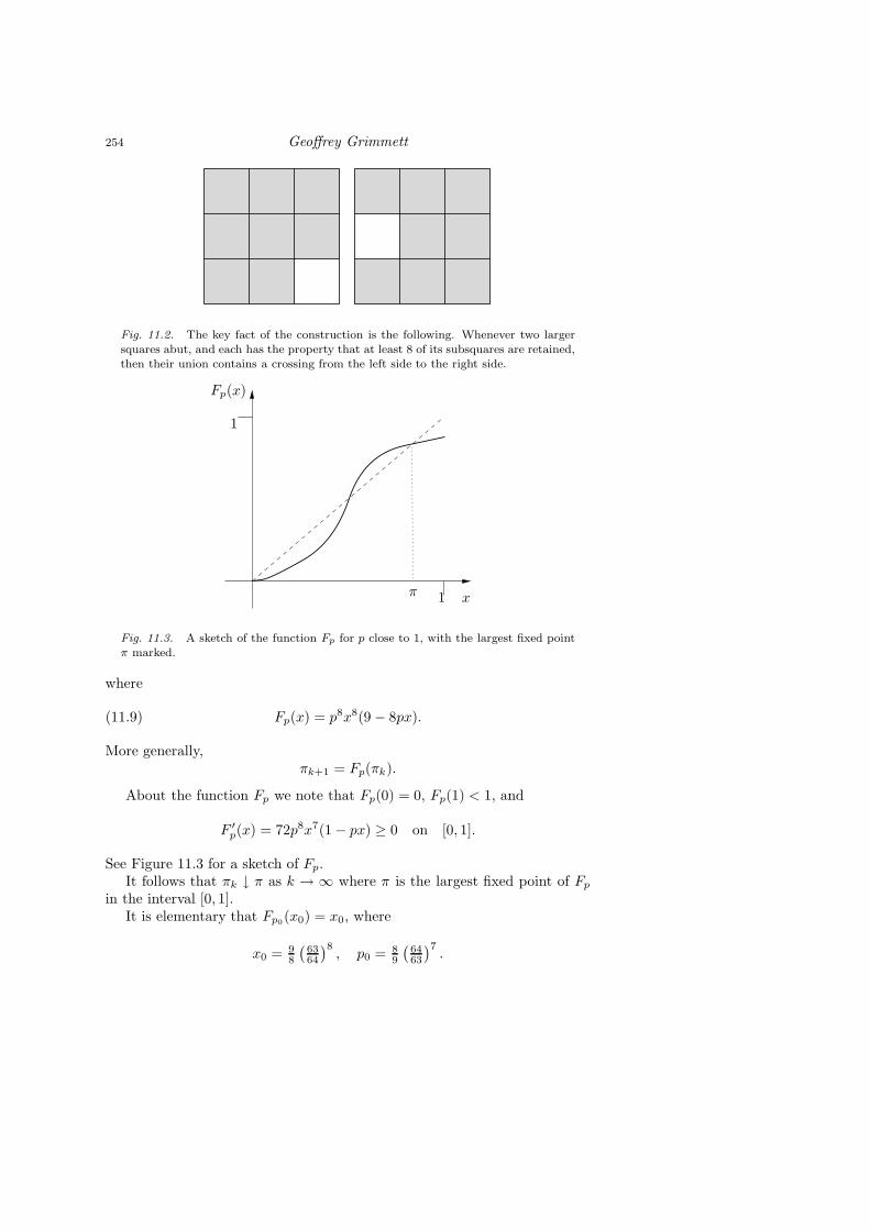
254 Geoffrey Grimmett
Fig. 11.2. The key fact of the construction is the following. Whenever two largersquares abut, and each has the property that at least 8 of its subsquares are retained,then their union contains a crossing from the left side to the right side.
Fp(x)
1
π 1 x
Fig. 11.3. A sketch of the function Fp for p close to 1, with the largest fixed pointπ marked.
where
(11.9) Fp(x) = p8x8(9 − 8px).
More generally,πk+1 = Fp(πk).
About the function Fp we note that Fp(0) = 0, Fp(1) < 1, and
F ′p(x) = 72p8x7(1 − px) ≥ 0 on [0, 1].
See Figure 11.3 for a sketch of Fp.It follows that πk ↓ π as k → ∞ where π is the largest fixed point of Fp
in the interval [0, 1].It is elementary that Fp0(x0) = x0, where
x0 = 98
(6364
)8, p0 = 8
9
(6463
)7.

Percolation and Disordered Systems 255
It follows that π(p0) ≥ x0, yielding θ(p0) > 0. Therefore pc ≤ p0, as requiredin (11.5).
The proof that θ(pc) > 0 is more delicate; see [113].
Consider now the more general setting in which the random step involvesreplacing a typical square of side-length M−k by a M×M grid of subsquaresof common side-length M−(k+1) (the above concerns the case M = 3). Forgeneral M , a version of the above argument yields that the correspondingcritical probability pc(M) satisfies pc(M) ≥M−2 and also
(11.10) pc(M) < 1 if M ≥ 3.
When M = 2, we need a special argument in order to obtain that pc(2) < 1,and this may be achieved by using the following coupling of the cases M = 2and M = 4 (see [91, 113]). Divide C0 into a 4 × 4 grid and do as follows. Atthe first stage, with probability p we retain all four squares in the top leftcorner; we do similarly for the three batches of four squares in each of theother three corners of C0. Now for the second stage: examine each subsquareof side-length 1
4 so far retained, and delete such a subsquare with probability p(different subsquares being treated independently). Note that the probabilitymeasure at the first stage dominates (stochastically) product measure withintensity π so long as (1−π)4 ≥ 1−p. Choose π to satisfy equality here. Thecomposite construction outlined above dominates (stochastically) a single
step of a 4 × 4 random fractal with parameter pπ = p(1 − (1 − p)
14
), which
implies that
pc(2)(1 − (1 − pc(2))
14
)≤ pc(4)
and therefore pc(2) < 1 by (11.10).
11.3 A Morphology
Random fractals have many phases, of which the existence of left-right cross-ings characterises only one. A weaker property than the existence of crossingsis that the projection of C onto the x-axis is the whole interval [0, 1]. Pro-jections of random fractals are of independent interest (see, for example, the‘digital sundial’ theorem of [131]). Dekking and Meester [113] have cast suchproperties within a more general morphology.
We write C for a random fractal in [0, 1]2 (such as that presented inSection 11.1). The projection of C is denoted as
πC = x ∈ R : (x, y) ∈ C for some y,
and λ denotes Lebesgue measure. We say that C lies in one of the followingphases if it has the stated property. A set is said to percolate if it contains aleft-right crossing of [0, 1]2; dimension is denoted by ‘dim’.
I. C = ∅ a.s.

256 Geoffrey Grimmett
II. P (C 6= ∅) > 0, dim(πC) = dimC a.s.III. dim(πC) < dimC a.s. on C 6= ∅, but λ(πC) = 0 a.s.IV. 0 < λ(πC) < 1 a.s. on C 6= ∅.V. P
(λ(πC) = 1
)> 0 but C does not percolate a.s.
VI. P (C percolates) > 0.In many cases of interest, there is a parameter p, and the ensuing fractal
moves through the phases, from I to VI, as p increases from 0 to 1. Theremay be critical values pM,N at which the model moves from Phase M toPhase N . In a variety of cases, the critical values pI,II, pII,III, pIII,IV can bedetermined exactly, whereas pIV,V and pV,VI can be much harder to find.
Here is a reasonably large family of random fractals. As before, theyare constructed by dividing a square into 9 equal subsquares. In this moregeneral system, we are provided with a probability measure µ, and we replacea square by the union of a random collection of subsquares sampled accordingto µ. This process is iterated on all relevant scales. Certain parameters areespecially relevant. Let σl be the number of subsquares retained from the lthcolumn, and let ml = E(σl) be its mean.
Theorem 11.11. We have that(a) C = ∅ if and only if
∑3l=1ml ≤ 1 (unless some σl is a.s. equal to 1),
(b) dim(πC) = dim(C) a.s. if and only if
3∑
l=1
ml logml ≤ 0,
(c) λ(πC) = 0 a.s. if and only if
3∑
l=1
logml ≤ 0.
For the proofs, see [112, 133]. Consequently, one may check the Phases I,II, III by a knowledge of the ml only.
Next we apply Theorem 11.11 to the random Cantor set of Section 11.1,to obtain that, for this model, pI,II = 1
9 , and we depart Phase II as p increases
through the value 13 . The system is never in Phase III (by Theorem 11.1(c))
or in Phase IV (by Theorem 1 of [133]). It turns out that pII,V = 13 and
12 < pV,VI < 1.
For the ‘random Sierpinski carpet’ (RSC) the picture is rather different.This model is constructed as the above but with one crucial difference: ateach iteration, the central square is removed with probability one, and theothers with probability 1 − p (see Figure 11.4). Applying Theorem 11.11 wefind that
pI,II = 18 , pII,III = 54−
14 , pIII,IV = 18−
13 ,

Percolation and Disordered Systems 257
Fig. 11.4. In the construction of the Sierpinski carpet, the middle square is alwaysdeleted.
and it happens that
12 < pIV,V ≤ 0.8085, 0.812 ≤ pV,VI ≤ 0.991.
See [113] for more details.We close this section with a conjecture which has received some attention.
Writing pc (resp. pc(RSC)) for the critical point of the random fractal ofSection 11.1 (resp. the random Sierpinski carpet), it is evident that pc ≤pc(RSC). Prove or disprove the strict inequality pc < pc(RSC).
11.4 Relationship to Brownian Motion
Peres [311] has discovered a link between fractal percolation and BrownianMotion, via a notion called ‘intersection-equivalence’. For a region U ⊆ Rd,we call two random sets B and C intersection-equivalent in U if
(11.12) P (B ∩ Λ 6= ∅) ≍ P (C ∩ Λ 6= ∅) for all closed Λ ⊆ U
(i.e., there exist positive finite constants c1, c2, possibly depending on U , suchthat
c1 ≤ P (B ∩ Λ 6= ∅)
P (C ∩ Λ 6= ∅)≤ c2
for all closed Λ ⊆ U).We apply this definition for two particular random sets. First, write B
for the range of Brownian Motion in Rd, starting at a point chosen uniformlyat random in the unit cube. Also, for d ≥ 3, let C be a random Cantor setconstructed by binary splitting (rather than the ternary splitting of Section11.1) and with parameter p = 22−d.
258 Geoffrey Grimmett
Theorem 11.13. Suppose that d ≥ 3. The random sets B and C are inter-section-equivalent.
A similar result is valid when d = 2, but with a suitable redefinition of therandom set C. This is achieved by taking different values of p at the differentstages of the construction, namely p = k/(k + 1) at the kth stage.
This correspondence is not only beautiful and surprising, but also use-ful. It provides a fairly straightforward route to certain results concerningintersections of random walks and Brownian Motions, for example. Con-versely, using the rotation-invariance of Brownian Motion, one may obtainresults concerning projections of the random Cantor set in other directionsthan onto an axis (thereby complementing results of [112], in the case of thespecial parameter-value given above).
The proof of Theorem 11.13 is analytical, and proceeds by utilising• classical potential theory for Brownian Motion,• the relationship between capacity and percolation for trees ([250]), and• the relationship between capacity on trees and capacity on an associ-
ated Euclidean space ([54, 308]).It is an attractive target to understand Theorem 11.13 via a coupling of thetwo random sets.

Percolation and Disordered Systems 259
12. ISING AND POTTS MODELS
12.1 Ising Model for Ferromagnets
In a famous experiment, a piece of iron is exposed to a magnetic field. Thefield increases from zero to a maximum, and then diminishes to zero. If thetemperature is sufficiently low, the iron retains some ‘residual magnetisation’,otherwise it does not. The critical temperature for this phenomenon is oftencalled the Curie point. In a famous scientific paper [195], Ising proposed amathematical model which may be phrased in the following way, using themodern idiom.
Let Λ be a box of Zd, say Λ = [−n, n]d. Each vertex in Λ is allocated a ran-dom spin according to a Gibbsian probability measure as follows. Since spinscome in two basic types, we take as sample space the set ΣΛ = −1,+1Λ,and we consider the probability measure πΛ which allocates a probability toa spin vector σ ∈ ΣΛ given by
(12.1) πΛ(σ) =1
ZΛexp−βHΛ(σ), σ ∈ ΣΛ,
where β = T−1 (the reciprocal of temperature, on a certain scale) and theHamiltonian HΛ : ΣΛ → R is given by
(12.2) HΛ(σ) = −∑
e=〈i,j〉
Jeσiσj − h∑
i
σi
for constants (Je) and h (called the ‘external field’) which parameterise theprocess. The sums in (12.2) are over all edges and vertices of Λ, respectively.
The measure (12.1) is said to arise from ‘free boundary conditions’, sincethe boundary spins have no special role. It turns out to be interesting to allowother types of boundary conditions. For any assignment γ : ∂Λ → −1,+1there is a corresponding probability measure πγΛ obtained by restricting thevector σ to the set of vectors which agree with γ on ∂Λ. In this way wemay obtain measures π+
Λ , π−Λ , and πf
Λ (with free boundary conditions) onappropriate subsets of ΣΛ.
For simplicity, we assume here that Je = J > 0 for all edges e. In this‘ferromagnetic’ case, measures of the form (12.1) prefer to see configurationsσ in which neighbouring vertices have like spins. The antiferromagnetic caseJ < 0 can be somewhat tricky.
Inspecting (12.1)–(12.2) with J > 0, we see that spins tend to align withthe sign of any external field h.
The following questions are basic.(a) What weak limits limΛ→Zd πγΛ exist for possible boundary conditions
γ? (This requires redefining πγΛ as a probability measure associated
with the sample space Σ = −1,+1Zd
.)

260 Geoffrey Grimmett
(b) Under what conditions on J, h, d is there a unique limit measure?(c) How may limit measures be characterised?(d) What are their properties; for example, at what rate do their correla-
tions decay over large distances?(e) Is there a phase transition?It turns out that there is a unique limit if either d = 1 or h 6= 0. There is
non-uniqueness when d ≥ 2, h = 0, and β is sufficiently large (i.e., β > T−1c
where Tc is the Curie point).A great deal is known about the Ising model; see, for example, [9, 129, 134,
149, 237] and many other sources. We choose here to follow a random-clusteranalysis, the details of which will follow.
The Ising model on L2 permits one of the famous exact calculations ofstatistical physics, following Onsager [299].
12.2 Potts Models
Whereas the Ising model permits two possible spin-values at each vertex,the Potts model permits a general number q ∈ 2, 3, . . .. The model wasintroduced by Potts [317] following an earlier paper of Ashkin and Teller [45].
Let q ≥ 2 be an integer, and take as sample space ΣΛ = 1, 2, . . . , qΛ
where Λ is given as before. This time we set
(12.3) πΛ(σ) =1
ZΛexp−βHΛ(σ), σ ∈ ΣΛ,
where
(12.4) HΛ(σ) = −J∑
e=〈i,j〉
δσi,σj
and δu,v is the Kronecker delta
δu,v =
1 if u = v,
0 otherwise.
External field is absent from this formulation, but can be introduced if re-quired by the addition to (12.4) of the term −h∑i δσi,1, which favours anarbitrarily chosen spin-value, being here the value 1.
The labelling 1, 2, . . . , q of the spin-values is of course arbitrary. The caseq = 2 is identical to the Ising model (without external field and with anamended value of J), since
σiσj = 2δσi,σj− 1 for σi, σj ∈ −1,+1.

Percolation and Disordered Systems 261
12.3 Random-Cluster Models
It was Fortuin and Kasteleyn who discovered that Potts models may berecast as ‘random-cluster models’. In doing so, they described a class ofmodels, including percolation, which merits attention in their own right, andthrough whose analysis we discover fundamental facts concerning Ising andPotts models. See [158] for a recent account of the relevant history andbibliography.
The neatest construction of random-cluster models from Potts models isthat reported in [127]. Let G = (V,E) be a finite graph, and define thesample spaces
Σ = 1, 2, . . . , qV , Ω = 0, 1E,
where q is a positive integer. We now define a probability mass function µon Σ × Ω by
(12.5) µ(σ, ω) ∝∏
e∈E
(1 − p)δω(e),0 + pδω(e),1δe(σ)
where 0 ≤ p ≤ 1, and
(12.6) δe(σ) = δσi,σjif e = 〈i, j〉 ∈ E.
Elementary calculations reveal the following facts.(a) Marginal on Σ. The marginal measure
µ(σ, ·) =∑
ω∈Ω
µ(σ, ω)
is given by
µ(σ, ·) ∝ exp
βJ∑
e
δe(σ)
where p = 1 − e−βJ . This is the Potts measure (12.3). Note thatβJ ≥ 0.
(b) Marginal on Ω. Similarly
µ(·, ω) =∑
σ∈Σ
µ(σ, ω) ∝∏
e
pω(e)(1 − p)1−ω(e)
qk(ω)
where k(ω) is the number of connected components (or ‘clusters’) ofthe graph with vertex set V and edge set η(ω) = e ∈ E : ω(e) = 1.
(c) The conditional measures . Given ω, the conditional measure on Σ isobtained by putting (uniformly) random spins on entire clusters of ω(of which there are k(ω)), which are constant on given clusters, andindependent between clusters. Given σ, the conditional measure on Ω
262 Geoffrey Grimmett
is obtained by setting ω(e) = 0 if δe(σ) = 0, and otherwise ω(e) = 1with probability p (independently of other edges).
In conclusion, the measure µ is a coupling of a Potts measure πβ,J on V ,together with a ‘random-cluster measure’
(12.7) φp,q(ω) ∝∏
e∈E
pω(e)(1 − p)1−ω(e)
qk(ω), ω ∈ Ω.
The parameters of these measures correspond to one another by the relationp = 1 − e−βJ . Since 0 ≤ p ≤ 1, this is only possible if βJ ≥ 0.
Why is this interesting? The ‘two-point correlation function’ of the Pottsmeasure πβ,J on G = (V,E) is defined to be the function τβ,J given by
τβ,J(i, j) = πβ,J(σi = σj) −1
q, i, j ∈ V.
The ‘two-point connectivity function’ of the random-cluster measure φ isφp,q(i ↔ j), i.e., the probability that i and j are in the same cluster of aconfiguration sampled according to φ. It turns out that these ‘two-pointfunctions’ are (except for a constant factor) the same.
Theorem 12.8. If q ∈ 2, 3, . . . and p = 1− e−βJ satisfies 0 ≤ p ≤ 1, then
τβ,J(i, j) = (1 − q−1)φp,q(i↔ j).
Proof. We have that
τβ,J(i, j) =∑
σ,ω
1σi=σj(σ) − q−1
µ(σ, ω)
=∑
ω
φp,q(ω)∑
σ
µ(σ | ω)
1σi=σj(σ) − q−1
=∑
ω
φp,q(ω)
(1 − q−1)1i↔j(ω) + 0 · 1i=j(ω)
= (1 − q−1)φp,q(i↔ j).
This fundamental correspondence implies that properties of Potts cor-relation can be mapped to properties of random-cluster connection. SincePottsian phase transition can be formulated in terms of correlation functions,this implies that information about percolative phase transition for random-cluster models is useful for studying Pottsian transitions. In doing so, westudy the ‘stochastic geometry’ of random-cluster models.
The random-cluster measure (12.7) was constructed under the assumptionthat q ∈ 2, 3, . . ., but (12.7) makes sense for any positive real q. Wehave therefore obtained a rich family of measures which includes percolation(q = 1) as well as the Ising (q = 2) and Potts measures.
Percolation and Disordered Systems 263
13. RANDOM-CLUSTER MODELS
13.1 Basic Properties
First we summarise some useful properties of random-cluster measures. LetG = (V,E) be a finite graph, and write ΩE = 0, 1E. The random-clustermeasure on ΩE , with parameters p, q satisfying 0 ≤ p ≤ 1 and q > 0, is givenby
φp,q(ω) =1
Z
∏
e∈E
pω(e)(1 − p)1−ω(e)
qk(ω), ω ∈ ΩE
where Z = ZG,p,q is a normalising constant, and k(ω) is the number ofconnected components of the graph (V, η(ω)), where η(ω) = e : ω(e) = 1 isthe set of ‘open’ edges.
Theorem 13.1. The measure φp,q satisfies the FKG inequality if q ≥ 1.
Proof. If p = 0, 1, the conclusion is obvious. Assume 0 < p < 1, and checkthe condition (5.2), which amounts to the assertion that
k(ω ∨ ω′) + k(ω ∧ ω′) ≥ k(ω) + k(ω′) for ω, ω′ ∈ ΩE .
This we leave as a graph-theoretic exercise.
Theorem 13.2 (Comparison Inequalities). We have that
φp′,q′ ≤ φp,q if p′ ≤ p, q′ ≥ q, q′ ≥ 1,
(13.3)
φp′,q′ ≥ φp,q ifp′
q′(1 − p′)≥ p
q(1 − p), q′ ≥ q, q′ ≥ 1.
(13.4)
Proof. Use Holley’s Inequality (Theorem 5.5) after checking condition (5.6).
In the next theorem, the role of the graph G is emphasised in the useof the notation φG,p,q. The graph G\e (resp. G.e) is obtained from G bydeleting (resp. contracting) the edge e.
Theorem 13.5 (Tower Property). Let e ∈ E.(a) The conditional measure of φG,p,q given ω(e) = 0 is φG\e,p,q.(b) The conditional measure of φG,p,q given ω(e) = 1 is φG.e,p,q.
Proof. This is an elementary calculation of conditional probabilities.
More details of these facts may be found in [26, 159, 162]. Another com-parison inequality may be found in [161].

264 Geoffrey Grimmett
13.2 Weak Limits and Phase Transitions
Let d ≥ 2, and Ω = 0, 1Ed
. The appropriate σ-field of Ω is the σ-field Fgenerated by the finite-dimensional sets. For ω ∈ Ω and e ∈ Ed, the edge eis called open if ω(e) = 1 and closed otherwise.
Let Λ be a finite box in Zd. For b ∈ 0, 1 define
ΩbΛ = ω ∈ Ω : ω(e) = b for e /∈ EΛ,
where EA is the set of edges of Ld joining pairs of vertices belonging to A.On ΩbΛ we define a random-cluster measure φbΛ,p,q as follows. Let 0 ≤ p ≤ 1and q > 0. Let
(13.6) φbΛ,p,q(ω) =1
ZbΛ,p,q
∏
e∈EΛ
pω(e)(1 − p)1−ω(e)
qk(ω,Λ)
where k(ω,Λ) is the number of clusters of (Zd, η(ω)) which intersect Λ (here,as before, η(ω) = e ∈ Ed : ω(e) = 1 is the set of open edges). The boundarycondition b = 0 (resp. b = 1) is sometimes termed ‘free’ (resp. ‘wired’).
Theorem 13.7. The weak limits
φbp,q = limΛ→Zd
φbΛ,p,q, b = 0, 1,
exist if q ≥ 1.
Proof. Let A be an increasing cylinder (= finite-dimensional) event. If Λ ⊆ Λ′
and Λ includes the ‘base’ of A, then
φ1Λ,p,q(A) = φ1
Λ′,p,q(A | all edges in EΛ′\Λ are open) ≥ φ1Λ′,p,q(A),
where we have used the tower property and the FKG inequality. Thereforethe limit limΛ→Zd φ1
Λ,p,q(A) exists by monotonicity. Since F is generated by
such events A, the weak limit φ1p,q exists. A similar argument is valid in the
case b = 0.
The measures φ0p,q and φ1
p,q are called ‘random-cluster measures’ on Ld
with parameters p and q. Another route to a definition of such measuresuses a type of Dobrushin–Lanford–Ruelle (DLR) formalism rather than weaklimits (see [162])10. There is a set of ‘DLR measures’ φ satisfying φ0
p,q ≤ φ ≤φ1p,q, whence there is a unique such measure if and only if φ0
p,q = φ1p,q.
10Let φξΛ,p,q be the random-cluster measure on Λ having boundary conditions inherited
from the configuration ξ off Λ. It is proved in [162] that any limit point φ of the family
of probability measures φξΛ,p,q : Λ ⊆ Zd, ξ ∈ Ω is a DLR measure whenever φ has the
property that the number I of infinite open clusters satisfies φ(I ≤ 1) = 1. It is an openproblem to decide exactly which weak limits are DLR measures (if not all).

Percolation and Disordered Systems 265
Henceforth we assume that q ≥ 1. Turning to the question of phase tran-sition, and remembering percolation, we define the percolation probabilities
(13.8) θb(p, q) = φbp,q(0 ↔ ∞), b = 0, 1,
i.e., the probability that 0 belongs to an infinite open cluster. The corre-sponding critical probabilities are given by
pbc(q) = supp : θb(p, q) = 0, b = 0, 1.
Faced possibly with two (or more) distinct critical probabilities, we presentthe following result, abstracted from [16, 158, 159, 162].
Theorem 13.9. Assume that d ≥ 2 and q ≥ 1. There exists a countablesubset P = Pq,d of [0, 1], possibly empty, such that φ0
p,q = φ1p,q if either
θ1(p, q) = 0 or p /∈ P.
Consequently, θ0(p, q) = θ1(p, q) if p does not belong to the countable setPq,d, whence p0
c(q) = p1c(q). Henceforth we refer to the critical value as pc(q).
It is believed that Pq,d = ∅ for small q (depending on the value of d), andthat Pq,d = pc(q) for large q; see the next section.
Next we prove the non-triviality of pc(q) for q ≥ 1 (see [16]).
Theorem 13.10. If d ≥ 2 and q ≥ 1 then 0 < pc(q) < 1.
Proof. We compare the case of general q with the case q = 1 (percolation).Using the comparison inequalities (Theorem 13.2), we find that
(13.11) pc(1) ≤ pc(q) ≤qpc(1)
1 + (q − 1)pc(1), q ≥ 1,
where pc(1) is the critical probability of bond percolation on Ld. Cf. Theorem
3.2.
We note that pc(q) is monotone non-decreasing in q, by use of the compar-ison inequalities. Actually it is strictly monotone and Lipschitz continuous(see [161]).
Finally we return to the Potts model, and we review the correspondenceof phase transitions. The relevant ‘order parameter’ of the Potts model isgiven by
M(βJ, q) = limΛ→Zd
π1
Λ,β,J
(σ(0) = 1
)− q−1
,
where π1Λ,β,J is a Potts measure on Λ ‘with boundary condition 1’. We may
think of M(βJ, q) as a measure of the degree to which the boundary condition‘1’ is noticed at the origin. By an application of Theorem 12.8 to a suitablegraph obtained from Λ, we have that
π1Λ,β,J
(σ(0) = 1
)− q−1 = (1 − q−1)φ1
Λ,p,q(0 ↔ ∂Λ)

266 Geoffrey Grimmett
where p = 1 − e−βJ . Therefore
M(βJ, q) = (1 − q−1) limΛ→Zd
φ1Λ,p,q(0 ↔ ∂Λ).
By an interchange of limits (which may be justified, see [16, 162]), we havethat11
limΛ→Zd
φ1Λ,p,q(0 ↔ ∂Λ) = θ1(p, q),
whence M(βJ, q) and θ1(p, q) differ only by the factor (1 − q−1).
13.3 First and Second Order Transitions
Let q ≥ 1 and 0 ≤ p ≤ 1. As before, φbp,q is the random-cluster measure
on Ld constructed according to the boundary condition b ∈ 0, 1. The
corresponding percolation probability is θb(p, q) = φbp,q(0 ↔ ∞). There is aphase transition at the point pc = pc(q). Much of the interest in Potts models(and therefore random-cluster models) has been directed at a dichotomy inthe type of phase transition, which depends apparently on whether q is smallor large. The following picture is credible but proved only in part.
(a) Small q, say 1 ≤ q < Q(d). It is believed that φ0p,q = φ1
p,q for all p, and
that θb(pc(q), q) = 0 for b = 0, 1. This will imply (see [162]) that there is aunique random-cluster measure, and that each θb(·, q) is continuous at thecritical point. Such a transition is sometimes termed ‘second order’. Thetwo-point connectivity function
(13.12) τbp,q(x, y) = φbp,q(x↔ y)
satisfies
(13.13) − 1
nlog τbp,q(0, ne1) → σ(p, q) as n→ ∞
where σ(p, q) > 0 if and only if p < pc(q). In particular σ(pc(q), q) = 0.
(b) Large q, say q > Q(d). We have that φ0p,q = φ1
p,q if and only if p 6=pc(q). When p = pc(q), then φ0
p,q and φ1p,q are the unique translation-
invariant random-cluster measures on Ld. Furthermore θ0(pc(q), q) = 0 andθ1(pc(q), q) > 0, which implies that θ1(·, q) is discontinuous at the criticalpoint. Such a transition is sometimes termed ‘first order’. The limit func-tion σ, given by (13.13) with b = 0, satisfies σ(pc(q), q) > 0, which is to saythat the measure φ0
p,q has exponentially decaying connectivities even at thecritical point. Trivially σ(p, q) = 0 when p > pc(q), and this discontinuity atpc(q) is termed the ‘mass gap’.
11We note that the corresponding limit for the free measure, limΛ→Zd φ0Λ,p,q(0 ↔
∂Λ) = θ0(p, q), has not been proved in its full generality; see [162, 315].

Percolation and Disordered Systems 267
It is further believed that Q(d) is non-increasing in d with
(13.14) Q(d) =
4 if d = 2
2 if d ≥ 6.
Some progress has been made towards verifying the main features of thispicture. When d = 2, special properties of two-dimensional space (particu-larly, a duality property) may be utilised (see Section 13.5). As for generalvalues of d, we have partial information when q = 1, q = 2, or q is sufficientlylarge. There is no full proof of a ‘sharp cut-off’ in the value of q, i.e., theexistence of a critical value Q(d) for q (even when d = 2, but see [192]).
Specifically, the following is known.
(c) When q = 1, it is elementary that there is a unique random-clustermeasure, namely product measure. Also, θ(pc(1), 1) = 0 if d = 2 or d ≥ 19(and perhaps for other d also). There is no mass gap, but σ(p, q) > 0 forp < pc(1). See [G].
(d) When q = 2, we have information via technology developed for the Isingmodel. For example, θ1(pc(2), 2) = 0 if d 6= 3. Also, σ(p, 2) > 0 if p < pc(2).See [13].
(e) When q is sufficiently large, the Pirogov–Sinai theory of contours may beapplied to obtain the picture described in (b) above. See [224, 226, 227, 256].
Further information about the above arguments is presented in Section13.5 for the special case of two dimensions.
13.4 Exponential Decay in the Subcritical Phase
The key theorem for understanding the subcritical phase of percolation statesthat long-range connections have exponentially decaying probabilities (The-orem 6.10). Such a result is believed to hold for all random-cluster modelswith q ≥ 1, but no full proof has been found. The result is known only whenq = 1, q = 2, or q is sufficiently large, and the three sets of arguments forthese cases are somewhat different from one another. As for results valid forall q (≥ 1), the best that is currently known is that the connectivity functiondecays exponentially whenever it decays at a sufficient polynomial rate. Wedescribe this result in this section; see [167] for more details.
As a preliminary we introduce another definition of a critical point. Let
(13.15) Y (p, q) = lim supn→∞
nd−1φ0
p,q
(0 ↔ ∂B(n)
)
and
(13.16) pg(q) = supp : Y (p, q) <∞
.

268 Geoffrey Grimmett
Evidently pg(q) ≤ pc(q), and it is believed that equality is valid here. Next,we define the kth iterate of (natural) logarithm by
λ1(n) = logn, λk(n) = log+λk−1(n) for k ≥ 2
where log+ x = max1, logx.We present the next theorem in two parts, and shall give a full proof of
part (a) only; for part (b), see [167].
Theorem 13.17. Let 0 < p < 1 and q ≥ 1, and assume that p < pg(q).(a) If k ≥ 1, there exists α = α(p, q, k) satisfying α > 0 such that
(13.18) φ0p,q
(0 ↔ ∂B(n)
)≤ exp
−αn/λk(n)
for all large n.
(b) If (13.18) holds, then there exists β = β(p, q) satisfying β > 0 suchthat
φ0p,q
(0 ↔ ∂B(n)
)≤ e−βn for all large n.
The spirit of the theorem is close to that of Hammersley [175] and Simon–Lieb [236, 331], who derived exponential estimates when q = 1, 2, subject toa hypothesis of finite susceptibility (i.e., that
∑x φ
0p,q(0 ↔ x) < ∞). The
latter hypothesis is slightly stronger than the assumption of Theorem 13.17when d = 2.
Underlying any theorem of this type is an inequality. In this case we usetwo, of which the first is a consequence of the following version of Russo’sformula, taken from [74].
Theorem 13.19. Let 0 < p < 1, q > 0, and let ψp be the correspondingrandom-cluster measure on a finite graph G = (V,E). Then
d
dpψp(A) =
1
p(1 − p)
ψp(N1A) − ψp(N)ψp(A)
for any event A, where N = N(ω) is the number of open edges of a configu-ration ω.
Here, ψp is used both as probability measure and expectation operator.
Proof. We express ψp(A) as
ψp(A) =
∑ω 1A(ω)πp(ω)∑
ω πp(ω)
where πp(ω) = pN(ω)(1−p)|E|−N(ω)qk(ω). Now differentiate throughout withrespect to p, and gather the terms to obtain the required formula.
Percolation and Disordered Systems 269
Lemma 13.20. Let 0 < p < 1 and q ≥ 1. For any non-empty increasingevent A,
d
dp
logψp(A)
≥ ψp(FA)
p(1 − p)
where
FA(ω) = inf
∑
e
(ω′(e) − ω(e)
): ω′ ≥ ω, ω′ ∈ A
.
Proof. It may be checked that FA1A = 0, and that N + FA is increasing.Therefore, by the FKG inequality,
ψp(N1A) − ψp(N)ψp(A) = ψp((N + FA)1A
)− ψp(N)ψp(A)
≥ ψp(FA)ψp(A).
Now use Theorem 13.19.
The quantity FA is central to the proof of Theorem 13.17. In the proof,we shall make use of the following fact. If A is increasing and A ⊆ B1 ∩B2 ∩· · · ∩ Bm, where the Bi are cylinder events defined on disjoint sets of edges,then
(13.21) FA ≥m∑
i=1
FBi.
Lemma 13.22. Let q ≥ 1 and 0 < r < s < 1. There exists a functionc = c(r, s, q), satisfying 1 < c <∞, such that
ψr(FA ≤ k) ≤ ckψs(A) for all k ≥ 0
and for all increasing events A.
Proof. We sketch this, which is similar to the so called ‘sprinkling lemma’ of[14]; see also [G, 167].
Let r < s. The measures ψr and ψs may be coupled together in a naturalway. That is, there exists a probability measure µ on Ω2
E = 0, 1E×0, 1Esuch that:
(a) the first marginal of µ is ψr,(b) the second marginal of µ is ψs,(c) µ puts measure 1 on the set of configurations (π, ω) ∈ Ω2
E such thatπ ≤ ω.
Furthermore µ may be found such that the following holds. There exists apositive number β = β(r, s, q) such that, for any fixed ξ ∈ ΩE and subset Bof edges (possibly depending on ξ), we have that
(13.23)µ((π, ω) : ω(e) = 1 for e ∈ B, π = ξ
)
µ((π, ω) : π = ξ
) ≥ β|B|.
270 Geoffrey Grimmett
That is to say, conditional on the first component of a pair (π, ω) sampledaccording to µ, the measure of the second component dominates a non-trivialproduct measure.
Now suppose that ξ (∈ ΩE) is such that FA(ξ) ≤ k, and find a set B =B(ξ) of edges, such that |B| ≤ k, and with the property that ξB ∈ A, whereξB is the configuration obtained from ξ by declaring all edges in B to beopen. By (13.23),
ψs(A) ≥∑
ξ:FA(ξ)≤k
µ((π, ω) : ω(e) = 1 for e ∈ B, π = ξ
)
≥ βkψr(FA ≤ k)
as required.
Proof of Theorem 13.17. (a) Write An = 0 ↔ ∂B(n) and ψp = φ0B(m),p,q
where p < pc = pc(q). We apply Lemma 13.20 (in an integrated form), andpass to the limit as m→ ∞, to obtain that the measures φp,q = φ0
p,q satisfy
(13.24) φr,q(An) ≤ φs,q(An) exp−4(s− r)φs,q(Fn)
, if r ≤ s,
where Fn = FAn(we have used Theorem 13.2(a) here, together with the fact
that Fn is a decreasing random variable).Similarly, by summing the corresponding inequality of Lemma 13.22 over
k, and letting m→ ∞, we find that
(13.25) φr,q(Fn) ≥ − logφs,q(An)
log c− c
c− 1if r < s.
We shall use (13.24) and (13.25) in an iterative scheme. At the first stage,assume r < s < t < pg = pg(q). Find c1(t) such that
(13.26) φp,q(An) ≤ c1(t)
nd−1for all n.
By (13.25),
φs,q(Fn) ≥ (d− 1) logn
log c+ O(1),
which we insert into (13.24) to obtain
(13.27) φr,q(An) ≤ c2(r)
nd−1+∆2(r)for all n,
and for some constants c2(r), ∆2(r) (> 0). This is an improvement over(13.26).

Percolation and Disordered Systems 271
At the next stages we shall need to work slightly harder. Fix a positiveinteger m, and let Ri = im for 0 ≤ i ≤ K where K = ⌊n/m⌋. Let Li =∂B(Ri) ↔ ∂B(Ri+1) and Hi = FLi
. By (13.21),
(13.28) Fn ≥K−1∑
i=0
Hi.
Now there exists a constant η (<∞) such that
(13.29) φp,q(Li) ≤ |∂B(Ri)|φp,q(Am) ≤ ηnd−1φp,q(Am)
for 0 ≤ i ≤ K − 1.Let r < s < pg, and let c2 = c2(s), ∆2 = ∆2(s) as in (13.27). From
(13.28)–(13.29),
φs,q(Fn) ≥K−1∑
i=0
φs,q(Li) ≥ K(1 − ηnd−1φp,q(Am)
)
≥ K(
1 − ηnd−1 c2md−1+∆2
).
We now choose m by
m =
(2ηc2)nd−11/(d−1+∆2)
(actually, an integer close to this value) to find that
φs,q(Fn) ≥ 12K ≥ Dn∆3
for some D > 0, 0 < ∆3 < 1. Substitute into (13.24) to obtain
(13.30) φr,q(An) ≤ exp−c3n∆3
for some positive c3 = c3(r), ∆3 = ∆3(r). This improves (13.27) substan-tially.
We repeat the last step, using (13.30) in place of (13.27), to obtain
(13.31) φr,q(An) ≤ exp
− c4n
(logn)∆4
if r < pg
for some c4 = c4(r) > 0 and 1 < ∆4 = ∆4(r) <∞.At the next stage, we use (13.28)–(13.29) more carefully. This time, set
m = (logn)2, and let r < s < t < pg. By (13.29) and (13.31),
φt,q(Li) ≤ ηnd−1 exp
− c4m
(logm)∆4

272 Geoffrey Grimmett
which, via Lemma 13.22, implies as in (13.25) that
φs,q(Hi) ≥D(logn)2
(log logn)∆4
for some D > 0. By (13.28), and the fact that K = ⌊n/m⌋,
φs,q(Fn) ≥ D′n
(log logn)∆4
for some D′ > 0. By (13.24),
φr,q(An) ≤ exp
− c5n
(log logn)∆4
.
Since ∆4 > 1, this implies the claim of the theorem with k = 1. The claimfor general k requires k − 1 further iterations of the argument.(b) We omit the proof of this part. The fundamental argument is taken from[138], and the details are presented in [167].
13.5 The Case of Two Dimensions
In this section we consider the case of random-cluster measures on the squarelattice L2. Such measures have a property of self-duality which generalisesthat of bond percolation. We begin by describing this duality.
Let G = (V,E) be a plane graph with planar dual Gd = (V d, Ed). Anyconfiguration ω ∈ ΩE gives rise to a dual configuration ωd ∈ ΩEd defined asfollows. If e (∈ E) is crossed by the dual edge ed (∈ Ed), we define ωd(ed) =1−ω(e). As usual, η(ω) denotes the set e : ω(e) = 1 of edges which are openin ω. By drawing a picture, one may be convinced that every face of (V, η(ω))contains a unique component of (V d, η(ωd)), and therefore the number f(ω)of faces (including the infinite face) of (V, η(ω)) satisfies f(ω) = k(ωd). SeeFigure 13.1. (Note that this definition of the dual configuration differs slightlyfrom that used earlier for two-dimensional percolation.)
The random-cluster measure on G is given by
φG,p,q(ω) ∝(
p
1 − p
)|η(ω)|
qk(ω).
Using Euler’s formula,
k(ω) = |V | − |η(ω)| + f(ω) − 1,
and the facts that f(ω) = k(ωd) and |η(ω)| + |η(ωd)| = |E|, we have that
φG,p,q(ω) ∝(q(1 − p)
p
)|η(ωd)|
qk(ωd),

Percolation and Disordered Systems 273
Fig. 13.1. A primal configuration ω (with solid lines) and its dual configuration ωd
(with dashed lines). The arrows join the given vertices of the dual to a dual vertexin the infinite face. Note that each face of the primal graph (including the infiniteface) contains a unique component of the dual graph.
which is to say that
(13.32) φG,p,q(ω) = φGd,pd,q(ωd) for ω ∈ ΩE ,
where the dual parameter pd is given according to
(13.33)pd
1 − pd=q(1 − p)
p.
The unique fixed point of the mapping p 7→ pd is easily seen to be given byp = κq where
κq =
√q
1 +√q.
If we keep track of the constants of proportionality in the above calcula-tion, we find that the partition function
ZG,p,q =∑
ω∈ΩE
p|η(ω)|(1 − p)|E\η(ω)|qk(ω)
satisfies the duality relation
(13.34) ZG,p,q = q|V |−1
(1 − p
pd
)|E|
ZGd,pd,q
which, when p = pd = κq, becomes
(13.35) ZG,κq,q = q|V |−1− 12 |E|ZGd,κq,q.
We shall find a use for this later.

274 Geoffrey Grimmett
Turning to the square lattice, let Λn = [0, n]2, whose dual graph Λdn may
be obtained from [−1, n]2 + (12 ,
12 ) by identifying all boundary vertices. This
implies by (13.32) that
(13.36) φ0Λn,p,q(ω) = φ1
Λdn,p
d,q(ωd)
for configurations ω on Λn (and with a small ‘fix’ on the boundary of Λdn).
Letting n→ ∞, we obtain that
(13.37) φ0p,q(A) = φ1
pd,q(Ad)
for all cylinder events A, where Ad = ωd : ω ∈ A.As a consequence of this duality, we may obtain as in the proof of Theorem
9.1 that
(13.38) θ0(κq, q
)= 0
(see [162, 345]), whence the critical value of the square lattice satisfies
(13.39) pc(q) ≥√q
1 +√q
for q ≥ 1.
It is widely believed that
pc(q) =
√q
1 +√q
for q ≥ 1.
This is known to hold when q = 1 (percolation), when q = 2 (Ising model),and for sufficiently large values of q. Following the route of the proof ofTheorem 9.1, it suffices to show that
φ0p,q
(0 ↔ ∂B(n)
)≤ e−nψ(p,q) for all n,
and for some ψ(p, q) satisfying ψ(p, q) > 0 when p < pc(q). (Actually, ratherless than exponential decay is required; it would be enough to have decay atrate n−1.) This was proved by the work of [13, 236, 331] when q = 2. When qis large, this and more is known. Let µ be the connective constant of L2, and
let Q =
12
(µ +
√µ2 − 4
)4. We have that 2.620 < µ < 2.696 (see [334]),
whence 21.61 < Q < 25.72. We set
ψ(q) =1
24log
(1 +
√q)4
qµ4
,
noting that ψ(q) > 0 if and only if q > Q.
Theorem 13.40. If d = 2 and q > Q then the following hold.(a) The critical point is given by pc(q) =
√q/(1 +
√q).

Percolation and Disordered Systems 275
Fig. 13.2. The dashed lines include an outer circuit Γ of the dual Bd.
(b) We have that θ1(pc(q), q) > 0.(c) For any ψ < ψ(q),
φ0pc(q),q
(0 ↔ ∂B(n)
)≤ e−nψ for all large n.
We stress that these conclusions may be obtained for general d (≥ 2)when q is sufficiently large (q > Q = Q(d)), as may be shown using so calledPirogov–Sinai theory (see [226]). In the case d = 2 presented here, the aboveduality provides a beautiful and simple proof. This proof is an adaptationand extension of that of [227].
Proof. Let B = B(n) = [−n, n]2 as usual, and let Bd = [−n, n− 1]2 + (12 ,
12 )
be those vertices of the dual of B(n) which lie inside B(n) (i.e., we omitthe vertex in the infinite face of B). We shall work with ‘wired’ boundaryconditions on B, and we let ω be a configuration on the edges of B. Acircuit Γ of Bd is called an outer circuit of a configuration ω if the followingproperties hold:
(a) all edges of Γ are open in the dual configuration ωd, which is to saythat they traverse closed edges of B,
(b) the origin of L2 is in the interior of Γ,(c) every vertex of B lying in the exterior of Γ, but within distance of
1/√
2 of some vertex of Γ, belongs to the same component of ω.See Figure 13.2 for an illustration of the meaning of ‘outer circuit’.

276 Geoffrey Grimmett
Each circuit Γ of Bd partitions the set EB of edges of B into three sets,being
E = edges of B exterior to Γ,I = edges of B interior to Γ,
Γ′ = edges of B crossing Γ.
The edges I form a connected subgraph of B.Our target is to obtain an upper bound for the probability that a given Γ is
an outer circuit. This we shall do by examining certain partition functions.Since no open component of ω contains points lying in both the exteriorand interior of an outer circuit, the event OC(Γ) = Γ is an outer circuitsatisfies, for any dual circuit Γ having 0 in its interior,
φ1B,p,q
(OC(Γ)
)=
1
Z1B,p,q
∑
ω
1OC(Γ)(ω)πp(ω)(13.41)
=1
Z1B,p,q
(1 − p)|Γ|Z1E(Γ)ZI
where πp(ω) = pN(ω)(1 − p)|E|−N(ω)qk(ω), Z1E(Γ) is the sum of πp(ω
′) overall ω′ ∈ 0, 1E with ‘1’ boundary conditions on ∂B and consistent with Γbeing an outer circuit (i.e., property (c) above), and ZI is the sum of πp(ω
′′)over all ω′′ ∈ 0, 1I.
Next we use duality. Let Id be the set of dual edges which cross the primaledges I, and let m be the number of vertices of B inside Γ. By (13.34),
(13.42) ZI = qm−1
(1 − p
pd
)|I|
Z1Id,pd,q
where pd satisfies (13.33), and where Z1Id,pd,q is the partition function for
dual configurations, having wired boundary conditions, on the set V d ofvertices incident to Id (i.e., all vertices of V d on its boundary are identified,as indicated in Figure 13.3).
We note two general facts about partition functions. First, for any graphG, ZG,p,q ≥ 1 if q ≥ 1. Secondly, Z·,p,q has a property of supermultiplicativitywhen q ≥ 1, which implies in particular that
Z1B,p,q ≥ Z1
E(Γ)Z1I∪Γ′,p,q
for any circuit Γ of Bd. (This is where we use property (c) above.)Let I∗ = Id + (1
2 ,12 ), where Id is thought of as a subset of R
2. Note fromFigure 13.3 that I∗ ⊆ I ∪Γ′. Using the two general facts above, we have that
(13.43) Z1B,p,q ≥ Z1
E(Γ)Z1I∗,p,q = Z1
E(Γ)Z1Id,p,q.

Percolation and Disordered Systems 277
Fig. 13.3. The interior edges I of Γ are marked in the leftmost picture, and the dualId in the centre picture (the vertices marked with a cross are identified as a single
vertex). The shifted set I∗ = Id + ( 12, 1
2) is drawn in the rightmost picture. Note
that I∗ ⊆ I ∪ Γ′.
Now assume that p =√q/(1 +
√q), so that p = pd. Then, by (13.41)–
(13.43) and (13.35),
φ1B,p,q
(OC(Γ)
)= (1 − p)|Γ|
Z1E(Γ)ZIZ1B,p,q
(13.44)
= (1 − p)|Γ|qm−1− 12 |I|
Z1E(Γ)Z1
Id,p,q
Z1B,p,q
≤ (1 − p)|Γ|qm−1− 12 |I|.
Since each vertex of B (inside Γ) has degree 4, we have that
4m = 2|I| + |Γ|,
whence
(13.45) φ1B,p,q
(OC(Γ)
)≤ (1 − p)|Γ|q
14 |Γ|−1 =
1
q
(q
(1 +√q)4
)|Γ|/4
.
The number of dual circuits of B having length l and containing the originin their interior is no greater than lal, where al is the number of self-avoidingwalks of L
2 beginning at the origin and having length l. Therefore
∑
Γ
φ1B,p,q
(OC(Γ)
)≤
∞∑
l=4
1
q
(q
(1 +√q)4
)l/4lal.
Now l−1 log al → µ as l → ∞, where µ is the connective constant of L2.Suppose now that q > Q, so that qµ4 < (1 +
√q)4. It follows that there
exists A(q) (<∞) such that
∑
Γ
φ1B,p,q
(OC(Γ)
)< A(q) for all n.
278 Geoffrey Grimmett
If A(q) < 1 (which holds for sufficiently large q), then
φ1B,p,q(0 ↔ ∂B) = φ1
B,p,q
(OC(Γ) occurs for no Γ
)
≥ 1 −A(q) > 0.
(We have used the assumption of wired boundary conditions here.) Thisimplies, by taking the limit n → ∞, that θ1(p, q) > 0 when p =
√q/(1 +√
q). Using (13.39), this implies parts (a) and (b) of the theorem, when q issufficiently large.
For general q > Q, we have only that A(q) < ∞. In this case, we find N(< n) such that ∑
Γ outside B(N)
φ1B,p,q
(OC(Γ)
)< 1
2
where Γ is said to be outside B(N) if it contains B(N) in its interior. Thisimplies that φ1
B,p,q
(B(N) ↔ ∂B
)≥ 1
2 . Let n → ∞, and deduce that
φ1p,q
(B(N) ↔ ∞
)≥ 1
2 , implying that θ1(p, q) > 0 as required.
Turning to part (c)12, let p = pd =√q/(1 +
√q) and n ≤ r. Let An
be the (cylinder) event that the point (12 ,
12 ) lies in the interior of an open
circuit of length at least n, this circuit having the property that its interioris contained in the interior of no open circuit having length strictly less thann. We have from (13.36) and (13.45) that
(13.46) φ0B(r),p,q(An) ≤
∞∑
m=n
mamq
(q
(1 +√q)4
)m/4for all large r.
[Here, we use the observation that, if An occurs in B(r), then there existsa maximal open circuit Γ of B(r) containing (1
2 ,12 ). In the dual of B(r), Γ
constitutes an outer circuit.]We write LRn for the event that there is an open crossing of the rectangle
Rn = [0, n]× [0, 2n] from its left to its right side, and we set λn = φ0p,q(LRn).
We may find a point x on the left side of Rn and a point y on the right sidesuch that
φ0p,q(x↔ y in Rn) ≥ λn
(2n+ 1)2.
By placing six of these rectangles side by side (as in Figure 13.4), we find bythe FKG inequality that
(13.47) φ0p,q
(x↔ x+ (6n, 0) in [0, 6n] × [0, 2n]
)≥(
λn(2n+ 1)2
)6
.
12The present proof was completed following a contribution by Ken Alexander, see [36]for related material.

Percolation and Disordered Systems 279
x
y
x+ (6n, 0)
Fig. 13.4. Six copies of a rectangle having width n and height 2n may be puttogether to make a rectangle with size 6n by 2n. If each is crossed by an open pathjoining the images of x and y, then the larger rectangle is crossed between its shortersides.
Fig. 13.5. If each of four rectangles having dimensions 6n by 2n is crossed by anopen path between its shorter sides, then the annulus contains an open circuit havingthe origin in its interior.
We now use four copies of the rectangle [0, 6n]×[0, 2n] to construct an annulusaround the origin (see Figure 13.5). If each of these copies contains an opencrossing, then the annulus contains a circuit. Using the FKG inequality again,we deduce that
(13.48) φ0p,q(A4n) ≥
(λn
(2n+ 1)2
)24
.
Finally, if 0 ↔ ∂B(n), then one of the four rectangles [0, n] × [−n, n],[−n, n] × [0, n], [−n, 0] × [−n, n], [−n, n] × [−n, 0] is traversed by an openpath betwen its two longer sides. This implies that
(13.49) φ0p,q
(0 ↔ ∂B(n)
)≤ 4λn.
Combining (13.46)–(13.49), we obtain that
φ0p,q
(0 ↔ ∂B(n)
)≤ 4
(2n+ 1)2φ0p,q(A4n)
1/24
≤ 4
(2n+ 1)2
∞∑
m=4n
mamq
(q
(1 +√q)4
)m/41/24
.
As before, m−1 log am → µ as m→ ∞, whence part (c) follows.

280 Geoffrey Grimmett
REFERENCES
1. Abraham, D. B., Fontes, L., Newman, C. M., and Piza, M. S. T.(1995). Surface deconstruction and roughening in the multi-zigguratmodel of wetting. Physical Review E 52, R1257–R1260.
2. Abraham, D. B. and Newman, C. M. (1988). Wetting in a threedimensional system: an exact solution. Physical Review Letters 61,1969–1972.
3. Abraham, D. B. and Newman, C. M. (1989). Surfaces and Peierlscontours: 3-d wetting and 2-d Ising percolation. Communications inMathematical Physics 125, 181–200.
4. Abraham, D. B. and Newman, C. M. (1990). Recent exact results onwetting. Wetting Phenomena (J. De Coninck and F. Dunlop, eds.),Lecture Notes in Physics, vol. 354, Springer, Berlin, pp. 13–21.
5. Abraham, D. B. and Newman, C. M. (1991). Remarks on a randomsurface. Stochastic Orders and Decision under Risk (K. Mosler andM. S. Scarsini, eds.), IMS Lecture Notes, Monograph Series, vol. 19,pp. 1–6.
6. Abraham, D. B. and Newman, C. M. (1991). The wetting transitionin a random surface model. Journal of Statistical Physics 63, 1097–1111.
7. Aharony, A. and Stauffer, D. (1991). Introduction to PercolationTheory (Second edition). Taylor and Francis.
8. Ahlfors, L. V. (1966). Complex Analysis. McGraw-Hill, New York.9. Aizenman, M. (1982). Geometric analysis of φ4 fields and Ising
models. Communications in Mathematical Physics 86, 1–48.10. Aizenman, M. (1995). The geometry of critical percolation and
conformal invariance. Proceedings STATPHYS 1995 (Xianmen) (HaoBai-lin, ed.), World Scientific.
11. Aizenman, M. (1997). On the number of incipient spanning clusters.Nuclear Physics B 485, 551–582.
12. Aizenman, M. and Barsky, D. J. (1987). Sharpness of the phasetransition in percolation models. Communications in MathematicalPhysics 108, 489–526.
13. Aizenman, M., Barsky, D. J., and Fernandez, R. (1987). The phasetransition in a general class of Ising-type models is sharp. Journal ofStatistical Physics 47, 343–374.
14. Aizenman, M., Chayes, J. T., Chayes, L., Frohlich, J, and Russo, L.(1983). On a sharp transition from area law to perimeter law in asystem of random surfaces. Communications in Mathematical Physics92, 19–69.
15. Aizenman, M., Chayes, J. T., Chayes, L., and Newman, C. M.(1987). The phase boundary in dilute and random Ising and Pottsferromagnets. Journal of Physics A: Mathematical and General 20,L313.

Percolation and Disordered Systems 281
16. Aizenman, M., Chayes, J. T., Chayes, L., and Newman, C. M. (1988).Discontinuity of the magnetization in one-dimensional 1/|x− y|2 Isingand Potts models. Journal of Statistical Physics 50, 1–40.
17. Aizenman, M. and Fernandez, R. (1986). On the critical behaviorof the magnetization in high-dimensional Ising models. Journal ofStatistical Physics 44, 393–454.
18. Aizenman, M. and Fernandez, R. (1988). Critical exponents for long-range interactions. Letters in Mathematical Physics 16, 39.
19. Aizenman, M. and Grimmett, G. R. (1991). Strict monotonicity forcritical points in percolation and ferromagnetic models. Journal ofStatistical Physics 63, 817–835.
20. Aizenman, M., Kesten, H., and Newman, C. M. (1987). Uniqueness ofthe infinite cluster and continuity of connectivity functions for short-and long-range percolation. Communications in Mathematical Physics111, 505–532.
21. Aizenman, M., Kesten, H., and Newman, C. M. (1987). Uniquenessof the infinite cluster and related results in percolation. PercolationTheory and Ergodic Theory of Infinite Particle Systems (H. Kesten,ed.), IMA Volumes in Mathematics and its Applications, vol. 8,Springer-Verlag, Berlin–Heidelberg–New York, pp. 13–20.
22. Aizenman, M., Klein, A., and Newman, C. M. (1993). Percolationmethods for disordered quantum Ising models. Phase Transitions:Mathematics, Physics, Biology . . . (R. Kotecky, ed.), World Scientific,Singapore, pp. 1–26.
23. Aizenman, M. and Lebowitz, J. (1988). Metastability in bootstrappercolation. Journal of Physics A: Mathematical and General 21,3801–3813.
24. Aizenman, M., Lebowitz, J., and Bricmont, J. (1987). Percolationof the minority spins in high-dimensional Ising models. Journal ofStatistical Physics 49, 859–865.
25. Aizenman, M. and Nachtergaele, B. (1994). Geometric aspects ofquantum spin states. Communications in Mathematical Physics 164,17–63.
26. Aizenman, M. and Newman, C. M. (1984). Tree graph inequalitiesand critical behavior in percolation models. Journal of StatisticalPhysics 36, 107–143.
27. Aldous, D. and Steele, J. M. (1992). Asymptotics for Euclideanminimal spanning trees on random points. Probability Theory andRelated Fields 92, 247–258.
28. Alexander, K. S. (1990). Lower bounds on the connectivity functionin all directions for Bernoulli percolation in two and three dimensions.Annals of Probability 18, 1547–1562.
29. Alexander, K. S. (1992). Stability of the Wulff construction andfluctuations in shape for large finite clusters in two-dimensionalpercolation. Probability Theory and Related Fields 91, 507–532.

282 Geoffrey Grimmett
30. Alexander, K. S. (1993). Finite clusters in high-density continuouspercolation: compression and sphericality. Probability Theory andRelated Fields 97, 35–63.
31. Alexander, K. S. (1993). A note on some rates of convergence in first-passage percolation. Annals of Applied Probability 3, 81–90.
32. Alexander, K. S. (1995). Simultaneous uniqueness of infinite graphs instationary random labeled graphs. Communications in MathematicalPhysics 168, 39–55.
33. Alexander, K. S. (1995). Percolation and minimal spanning forests ininfinite graphs. Annals of Probability 23, 87–104.
34. Alexander, K. S. (1997). Approximation of subadditive functions andconvergence rates in limiting-shape results. Annals of Probability 25,30–55.
35. Alexander, K. S. (1996). The RSW theorem for continuum percolationand the CLT for Euclidean minimal spanning trees. Annals of AppliedProbability 6, 466–494.
36. Alexander, K. S. (1998). On weak mixing in lattice models. ProbabilityTheory and Related Fields 110, 441–471.
37. Alexander, K. S., Chayes, J. T., and Chayes, L. (1990). The Wulffconstruction and asymptotics of the finite cluster distribution for two-dimensional Bernoulli percolation. Communications in MathematicalPhysics 131, 1–50.
38. Alexander, K. S. and Molchanov, S. A. (1994). Percolation of levelsets for two-dimensional random fields with lattice symmetry. Journalof Statistical Physics 77, 627–643.
39. Andjel, E. (1993). Characteristic exponents for two-dimensionalbootstrap percolation. Annals of Probability 21, 926–935.
40. Andjel, E. and Schinazi, R. (1996). A complete convergence theoremfor an epidemic model. Journal of Applied Probability 33, 741–748.
41. Antal, P. and Pisztora, A. (1996). On the chemical distance forsupercritical Bernoulli percolation. Annals of Probability 24, 1036–1048.
42. Appel, M. J. and Wierman, J. C. (1987). On the absence of ABpercolation in bipartite graphs. Journal of Physics A: Mathematicaland General 20, 2527–2531.
43. Appel, M. J. and Wierman, J. C. (1987). Infinite AB percolationclusters exist on the triangular lattice. Journal of Physics A:Mathematical and General 20, 2533–2537.
44. Appel, M. J. and Wierman, J. C. (1993). AB percolation on bonddecorated graphs. Journal of Applied Probability 30, 153–166.
45. Ashkin, J. and Teller, E. (1943). Statistics of two-dimensional latticeswith four components. The Physical Review 64, 178–184.
46. Barlow, M. T., Pemantle, R., and Perkins, E. (1997). Diffusion-limitedaggregation on a homogenous tree. Probability Theory and RelatedFields 107, 1–60.

Percolation and Disordered Systems 283
47. Barsky, D. J. and Aizenman, M. (1991). Percolation critical exponentsunder the triangle condition. Annals of Probability 19, 1520–1536.
48. Barsky, D. J., Grimmett, G. R., and Newman, C. M. (1991).Dynamic renormalization and continuity of the percolation transitionin orthants. Spatial Stochastic Processes (K. S. Alexander andJ. C. Watkins, eds.), Birkhauser, Boston, pp. 37–55.
49. Barsky, D. J., Grimmett, G. R., and Newman, C. M. (1991).Percolation in half spaces: equality of critical probabilities andcontinuity of the percolation probability. Probability Theory andRelated Fields 90, 111–148.
50. Benjamini, I. (1996). Percolation on groups, preprint.51. Benjamini, I. and Kesten, H. (1995). Percolation of arbitrary words in
0, 1N. Annals of Probability 23, 1024–1060.52. Benjamini, I., Pemantle, R., and Peres, Y. (1995). Martin capacity for
Markov chains. Annals of Probability 23, 1332–1346.53. Benjamini, I., Pemantle, R., and Peres, Y. (1998). Unpredictable
paths and percolation. Annals of Probability 26, 1198–1211.54. Benjamini, I. and Peres, Y. (1992). Random walks on a tree and
capacity in the interval. Annales de l’Institut Henri Poincare:Probabilites et Statistiques 28, 557–592.
55. Benjamini, I. and Peres, Y. (1994). Tree-indexed random walks ongroups and first passage percolation. Probability Theory and RelatedFields 98, 91–112.
56. Benjamini, I. and Schramm, O. (1998). Conformal invariance ofVoronoi percolation. Communications in Mathematical Physics 197,75–107.
57. Berg, J. van den (1985). Disjoint occurrences of events: results andconjectures. Particle Systems, Random Media and Large Deviations(R. T. Durrett, ed.), Contemporary Mathematics no. 41, AmericanMathematical Society, Providence, R. I., pp. 357–361.
58. Berg, J. van den (1993). A uniqueness condition for Gibbs measures,with application to the 2-dimensional Ising anti-ferromagnet.Communications in Mathematical Physics 152, 161–166.
59. Berg, J. van den (1997). A constructive mixing condition for 2-DGibbs measures with random interactions. Annals of Probability 25,1316–1333.
60. Berg, J. van den (1996). A note on disjoint-occurrence inequalities formarked Poisson point processes. Journal of Applied Probability 33,420–426.
61. Berg, J. van den (1997). Some reflections on disjoint occurrences ofevents, preprint.
62. Berg, J. van den and Ermakov, A. (1996). A new lower bound for thecritical probability of site percolation on the square lattice. RandomStructures and Algorithms, 199–212.
284 Geoffrey Grimmett
63. Berg, J. van den and Fiebig, U. (1987). On a combinatorial conjectureconcerning disjoint occurrences of events. Annals of Probability 15,354–374.
64. Berg, J. van den, Grimmett, G. R., and Schinazi, R. B. (1998).Dependent random graphs and spatial epidemics. Annals of AppliedProbability 8, 317–336.
65. Berg, J. van den and Keane, M. (1985). On the continuity of thepercolation probability function. Particle Systems, Random Media andLarge Deviations (R. T. Durrett, ed.), Contemporary MathematicsSeries, vol. 26, AMS, Providence, R. I., pp. 61–65.
66. Berg, J. van den and Kesten, H. (1985). Inequalities with applicationsto percolation and reliability. Journal of Applied Probability 22, 556–569.
67. Berg, J. van den and Kesten, H. (1993). Inequalities for the timeconstant in first-passage percolation. Advances in Applied Probability3, 56–80.
68. Berg, J. van den and Maes, C. (1994). Disagreement percolation inthe study of Markov fields. Annals of Probability 22, 749–763.
69. Berg, J. van den and Meester, R. (1991). Stability properties of a flowprocess in graphs. Random Structures and Algorithms 2, 335–341.
70. Berg, J. van den and Steif, J. (1994). Percolation and the hard-corelattice gas model. Stochastic Processes and their Applications 49, 179–197.
71. Bezuidenhout, C. E. and Grimmett, G. R. (1990). The critical contactprocess dies out. Annals of Probability 18, 1462–1482.
72. Bezuidenhout, C. E. and Grimmett, G. R. (1991). Exponential decayfor subcritical contact and percolation processes. Annals of Probability19, 984–1009.
73. Bezuidenhout, C. E. and Grimmett, G. R. (1999). A central limittheorem for random walks in random labyrinths. Annales de l’InstitutHenri Poincare: Probabilites et Statistiques 35, 631683.
74. Bezuidenhout, C. E., Grimmett, G. R., and Kesten, H. (1993). Strictinequality for critical values of Potts models and random-clusterprocesses. Communications in Mathematical Physics 158, 1–16.
75. Bezuidenhout, C. E., Grimmett, G. R., and Loffler, A. (1996).Minimal spanning tree analysis of site percolation clusters. Journalof Statistical Physics 92, 1–34.
76. Bollobas, B., Grimmett, G. R., and Janson, S. (1996). The random-cluster process on the complete graph. Probability Theory and RelatedFields 104, 283–317.
77. Borgs, C. and Chayes, J. T. (1996). The covariance matrix of thePotts model: a random cluster analysis. Journal of Statistical Physics82, 1235–1297.

Percolation and Disordered Systems 285
78. Borgs, C., Chayes, J. T., Kesten, H., and Spencer, J. (1996). Thebirth of the infinite cluster. Communications in Mathematical Physics224, 153–204.
79. Bramson, M., Durrett, R. T., and Schonmann, R. H. (1991). Thecontact process in a random environment. Annals of Probability 19,960–983.
80. Broadbent, S. R. and Hammersley, J. M. (1957). Percolation processesI. Crystals and mazes. Proceedings of the Cambridge PhilosophicalSociety 53, 629–641.
81. Bunimovitch, L. A. and Troubetzkoy, S. E. (1992). Recurrenceproperties of Lorentz lattice gas cellular automata. Journal ofStatistical Physics 67, 289–302.
82. Burton, R. M. and Keane, M. (1989). Density and uniqueness inpercolation. Communications in Mathematical Physics 121, 501–505.
83. Burton, R. M. and Meester, R. (1993). Long range percolation instationary point processes. Random Structures and Algorithms 4, 177–190.
84. Burton, R. M. and Pemantle, R. (1993). Local characteristics, entropyand limit theorems for uniform spanning trees and domino tilings viatransfer-impedances. Annals of Probability 21, 1329–1371.
85. Campanino, M., Chayes, J. T., and Chayes, L. (1991). Gaussianfluctuations of connectivities in the subcritical regime of percolation.Probability Theory and Related Fields 88, 269–341.
86. Cardy, J. (1992). Critical percolation in finite geometries. Journal ofPhysics A: Mathematical and General 25, L201.
87. Chayes, J. T. and Chayes, L. (1987). The mean field bound for theorder parameter of Bernoulli percolation,. Percolation Theory andErgodic Theory of Infinite Particle Systems (H. Kesten, ed.), Springer-Verlag, New York, pp. 49–71.
88. Chayes, J. T. and Chayes, L. (1987). On the upper critical dimensionof Bernoulli percolation,. Communications in Mathematical Physics113, 27–48.
89. Chayes, J. T. and Chayes, L. (1989). The large-N limit of thethreshold values in Mandelbrot’s fractal percolation process. Journalof Physics A: Mathematical and General 22, L501–L506.
90. Chayes, J. T., Chayes, L., and Durrett, R. T. (1986). Critical behaviorof the two-dimensional first passage time. Journal of StatisticalPhysics 45, 933–948.
91. Chayes, J. T., Chayes, L., and Durrett, R. T. (1988). Connectivityproperties of Mandelbrot’s percolation process. Probability Theory andRelated Fields 77, 307–324.
92. Chayes, J. T., Chayes, L., Fisher, D. S., and Spencer, T. (1989).Correlation length bounds for disordered Ising ferromagnets.Communications in Mathematical Physics 120, 501–523.
286 Geoffrey Grimmett
93. Chayes, J. T., Chayes, L., Grannan, E., and Swindle, G. (1991).Phase transitions in Mandelbrot’s percolation process in 3 dimensions.Probability Theory and Related Fields 90, 291–300.
94. Chayes, J. T., Chayes, L., Grimmett, G. R., Kesten, H., andSchonmann, R. H. (1989). The correlation length for the high densityphase of Bernoulli percolation. Annals of Probability 17, 1277–1302.
95. Chayes, J. T., Chayes, L., and Kotecky, R. (1995). The analysisof the Widom–Rowlinson model by stochastic geometric methods.Communications in Mathematical Physics 172, 551–569.
96. Chayes, J. T., Chayes, L., and Newman, C M. (1987). Bernoullipercolation above threshold: an invasion percolation analysis. Annalsof Probability 15, 1272–1287.
97. Chayes, J. T., Chayes, L., and Schonmann, R. H. (1987). Exponentialdecay of connectivities in the two dimensional Ising model. Journal ofStatistical Physics 49, 433–445.
98. Chayes, L. (1991). On the critical behavior of the first passage time ind = 3. Helvetica Physica Acta 64, 1055–1069.
99. Chayes, L. (1993). The density of Peierls contours in d = 2 and theheight of the wedding cake. Journal of Physics A: Mathematical andGeneral 26, L481–L488.
100. Chayes, L. (1995). On the absence of directed fractal percolation.Journal of Physics A: Mathematical and General 28, L295–L301.
101. Chayes, L. (1995). Aspects of the fractal percolation process. FractalGeometry and Stochastics (C. Bandt, S. Graf and M. Zahle, eds.),Birkhauser, Boston, pp. 113–143.
102. Chayes, L. (1996). On the length of the shortest crossing in thesuper-critical phase of Mandelbrot’s percolation process. StochasticProcesses and their Applications 61, 25–43.
103. Chayes, L. (1996). Percolation and ferromagnetism on Z2: the q-statePotts cases. Stochastic Processes and their Applications 65, 209–216.
104. Chayes, L., Kotecky, R., and Shlosman, S. B. (1995). Aggregationand intermediate phases in dilute spin-systems. Communications inMathematical Physics 171, 203–232.
105. Chayes, L. and Winfield, C. (1993). The density of interfaces: a newfirst passage problem. Journal of Applied Probability 30, 851–862.
106. Chow, Y. S. and Teicher, H. (1978). Probability Theory. Springer,Berlin.
107. Clifford, P. (1990). Markov random fields in statistics. Disorder inPhysical Systems (G. R. Grimmett and D. J. A. Welsh, eds.), OxfordUniversity Press, Oxford, pp. 19–32.
108. Cohen, E. G. D. (1991). New types of diffusions in lattice gas cellularautomata. Microscopic Simulations of Complex HydrodynamicalPhenomena (M. Mareschal and B. L. Holian, eds.), Plenum Press,New York, pp. 137–152.

Percolation and Disordered Systems 287
109. Cohen, E. G. D. and Wang, F. (1995). New results for diffusion inLorentz lattice gas cellular automata. Journal of Statistical Physics81, 445–466.
110. Cohen, E. G. D. and Wang, F. (1995). Novel phenomena in Lorentzlattice gases. Physica A 219, 56–87.
111. Cox, J. T., Gandolfi, A., Griffin, P., and Kesten, H. (1993). Greedylattice animals I: Upper bounds. Advances in Applied Probability 3,1151–1169.
112. Dekking, F. M. and Grimmett, G. R. (1988). Superbranchingprocesses and projections of random Cantor sets. Probability Theoryand Related Fields 78, 335–355.
113. Dekking, F. M. and Meester, R. W. J. (1990). On the structure ofMandelbrot’s percolation process and other random Cantor sets.Journal of Statistical Physics 58, 1109–1126.
114. DeMasi, A., Ferrari, P. A., Goldstein, S., and Wick, W. D. (1985).Invariance principle for reversible Markov processes with applicationto diffusion in the percolation regime. Particle Systems, RandomMedia and Large Deviations (R. T. Durrett, ed.), ContemporaryMathematics no. 41, American Mathematical Society, Providence,R. I., pp. 71–85.
115. DeMasi, A., Ferrari, P. A., Goldstein, S., and Wick, W. D. (1989).An invariance principle for reversible Markov processes. Applicationsto random motions in random environments. Journal of StatisticalPhysics 55, 787–855.
116. Deuschel, J.-D. and Pisztora, A. (1996). Surface order large deviationsfor high-density percolation. Probability Theory and Related Fields104, 467–482.
117. Doyle, P. G. and Snell, E. L. (1984). Random Walks and ElectricNetworks. Carus Mathematical Monograph no. 22. AMA, Washington,D. C.
118. Durrett, R. T. (1988). Lecture Notes on Particle Systems andPercolation. Wadsworth and Brooks/Cole, Pacific Grove, California.
119. Durrett, R. T. (1991). The contact process, 1974–1989. Mathematicsof Random Media Blacksburg, VA, Lectures in Applied Mathematics,vol. 27, AMS, pp. 1–18.
120. Durrett, R. T. (1995). Ten lectures on particle systems. Ecole d’Etede Probabilites de Saint Flour XXIII-1993 (P. Bernard, ed.), LectureNotes in Mathematics no. 1608, Springer, Berlin, pp. 97–201.
121. Durrett, R. T. and Kesten, H. (1990). The critical parameter forconnectedness of some random graphs. A Tribute to Paul Erdos(A. Baker, B. Bollobas, and A. Hajnal, eds.), Cambridge UniversityPress, Cambridge, pp. 161–176.
122. Durrett, R. T. and Neuhauser, C. (1991). Epidemics with recovery.Advances in Applied Probability 1, 189–206.

288 Geoffrey Grimmett
123. Durrett, R. T. and Schonmann, R. H. (1988). The contact process ona finite set II. Annals of Probability 16, 1570–1583.
124. Durrett, R. T. and Schonmann, R. H. (1988). Large deviations for thecontact process and two dimensional percolation. Probability Theoryand Related Fields 77, 583–603.
125. Durrett, R. T., Schonmann, R. H., and Tanaka, N. I. (1989). Thecontact process on a finite set III. The critical case. Annals ofProbability 17, 1303–1321.
126. Durrett, R. T., Schonmann, R. H., and Tanaka, N. I. (1989).Correlation lengths for oriented percolation. Journal of StatisticalPhysics 55, 965–979.
127. Edwards, R. G. and Sokal, A. D. (1988). Generalization of theFortuin–Kasteleyn–Swendsen–Wang representation and Monte Carloalgorithm. The Physical Review D 38, 2009–2012.
128. Ehrenfest, P. (1959). Collected Scientific Papers (M. J. Klein, ed.).North-Holland, Amsterdam.
129. Enter, A. C. D. van and Hollander, F. den (1993). Interacting particlesystems and Gibbs measures, Lecture notes for Master Class 1992–1993, Mathematical Research Institute, The Netherlands.
130. Falconer, K. J. (1986). Random fractals. Mathematical Proceedings ofthe Cambridge Philosophical Society 100, 559–582.
131. Falconer, K. J. (1986). Sets with prescribed projections and Nikodymsets. Proceedings of the London Mathematical Society 53, 48–64.
132. Falconer, K. J. (1989). Projections of random Cantor sets. Journal ofTheoretical Probability 2, 65–70.
133. Falconer, K. J. and Grimmett, G. R. (1992). On the geometry ofrandom Cantor sets and fractal percolation. Journal of TheoreticalProbability 5, 465–485; Erratum (1994) 7, 209–210.
134. Fernandez, R., Frohlich, J., and Sokal, A. D. (1992). Random Walks,Critical Phenomena, and Triviality in Quantum Field Theory.Springer-Verlag, Berlin.
135. Fill, J. and Pemantle, R. (1992). Oriented percolation, first-passagepercolation and covering times for Richardson’s model on the n-cube.Annals of Applied Probability 3, 593–629.
136. Fiocco, M. and Zwet, W. R. van (1996). Parameter estimation for thesupercritical contact process. Bernoulli 9, 1071–1092.
137. Fisher, M. E. (1961). Critical probabilities for cluster size andpercolation problems. Journal of Mathematical Physics 2, 620–627.
138. Fontes, L. and Newman, C. M. (1993). First passage percolation forrandom colorings of Zd. Annals of Applied Probability 3, 746–762;Erratum 4, 254.
139. Fortuin, C. M. (1971). On the random-cluster model. Doctoral thesis,University of Leiden.
140. Fortuin, C. M. (1972). On the random cluster model. II. Thepercolation model. Physica 58, 393–418.
Percolation and Disordered Systems 289
141. Fortuin, C. M. (1972). On the random cluster model. III. The simplerandom-cluster process. Physica 59, 545–570.
142. Fortuin, C. M. and Kasteleyn, P. W. (1972). On the random clustermodel. I. Introduction and relation to other models. Physica 57, 536–564.
143. Fortuin, C. M., Kasteleyn, P. W., and Ginibre, J. (1971). Correlationinequalities on some partially ordered sets. Communications inMathematical Physics 22, 89–103.
144. Friedgut, E. and Kalai, G. (1996). Every monotone graph propertyhas a sharp threshold. Proceedings of the American MathematicalSociety 124, 2993–3002.
145. Gandolfi, A., Grimmett, G. R., and Russo, L. (1988). On theuniqueness of the infinite open cluster in the percolation model.Communications in Mathematical Physics 114, 549–552.
146. Gandolfi, A., Keane, M., and Newman, C. M. (1992). Uniquenessof the infinite component in a random graph with applications topercolation and spin glasses. Probability Theory and Related Fields92, 511–527.
147. Gandolfi, A. and Kesten, H. (1994). Greedy lattice animals II: Lineargrowth. Advances in Applied Probability 4, 76–107.
148. Gandolfi, A., Newman, C. M., and Stein, D. L. (1993). Exotic statesin long range spin glasses. Communications in Mathematical Physics157, 371–387.
149. Georgii, H.-O. (1988). Gibbs Measures and Phase Transitions. Walterde Gruyter, Berlin.
150. Gordon, D. M. (1991). Percolation in high dimensions. Bulletin of theLondon Mathematical Society 44, 373–384.
151. Graf, S. (1987). Statistically self-similar fractals. Probability Theoryand Related Fields 74, 357–392.
152. Graf, S., Mauldin, R. D., and Williams, S. C. (1987). Exact Hausdorffdimension in random recursive constructions. Memoirs of theAmerican Mathematical Society 381.
153. Griffeath, D. (1979). Additive and Cancellative Interacting ParticleSystems. Lecture Notes in Mathematics, vol. 724. Springer, Berlin.
154. Grimmett, G. R. (1978). The rank functions of large random lattices.Journal of London Mathematical Society 18, 567–575.
155. Grimmett, G. R. (1989). Percolation. Springer-Verlag, Berlin.156. Grimmett, G. R. (1993). Differential inequalities for Potts and
random-cluster processes. Cellular Automata and Cooperative Systems(N. Boccara et al., eds.), Kluwer, Dordrecht, pp. 227–236.
157. Grimmett, G. R. (1994). Potts models and random-cluster processeswith many-body interactions. Journal of Statistical Physics 75, 67–121.

290 Geoffrey Grimmett
158. Grimmett, G. R. (1994). The random-cluster model. Probability,Statistics and Optimisation (F. P. Kelly, ed.), John Wiley & Sons,Chichester, pp. 49–63.
159. Grimmett, G. R. (1994). Percolative problems. Probability and PhaseTransition (G. R. Grimmett, ed.), Kluwer, Dordrecht, pp. 69–86.
160. Grimmett, G. R. (1994). Probability and Phase Transition. editor.Kluwer, Dordrecht.
161. Grimmett, G. R. (1995). Comparison and disjoint-occurrenceinequalities for random-cluster models. Journal of Statistical Physics78, 1311–1324.
162. Grimmett, G. R. (1995). The stochastic random-cluster process andthe uniqueness of random-cluster measures. Annals of Probability 23,1461–1510.
163. Grimmett, G. R., Kesten, H., and Zhang, Y. (1993). Random walk onthe infinite cluster of the percolation model. Probability Theory andRelated Fields 96, 33–44.
164. Grimmett, G. R. and Marstrand, J. M. (1990). The supercriticalphase of percolation is well behaved. Proceedings of the Royal Society(London), Series A 430, 439–457.
165. Grimmett, G. R., Menshikov, M. V., and Volkov, S. E. (1996).Random walks in random labyrinths. Markov Processes and RelatedFields 2, 69–86.
166. Grimmett, G. R. and Newman, C. M. (1990). Percolation in ∞ + 1dimensions. Disorder in Physical Systems (G. R. Grimmett andD. J. A. Welsh, eds.), Clarendon Press, Oxford, pp. 167–190.
167. Grimmett, G. R. and Piza, M. S. T. (1997). Decay of correlationsin subcritical Potts and random-cluster models. Communications inMathematical Physics 189, 465–480.
168. Grimmett, G. R. and Stacey, A. M. (1998). Inequalities for criticalprobabilities of site and bond percolation. Annals of Probability 26,1788–1812.
169. Grimmett, G. R. and Stirzaker, D. R. (1992). Probability and RandomProcesses. Oxford University Press, Oxford.
170. Haggstrom, O. (1996). The random-cluster model on a homogeneoustree. Probability Theory and Related Fields 104, 231–253.
171. Haggstrom, O. and Meester, R. (1995). Asymptotic shapes instationary first passage percolation. Annals of Probability 23, 1511–1522.
172. Haggstrom, O. and Meester, R. (1996). Nearest neighbour and hardsphere models in continuum percolation. Random Structures andAlgorithms, 295–315.
173. Haggstrom, O. and Pemantle, R. (1998). First-passage percolation anda model for competing spatial growth. Journal of Applied Probability,683–692.

Percolation and Disordered Systems 291
174. Haggstrom, O., Peres, Y., and Steif, J. (1997). Dynamical percolation.Annales de l’Institut Henri Poincare: Probabilites et Statistiques 33,497–528.
175. Hammersley, J. M. (1957). Percolation processes. Lower bounds forthe critical probability. Annals of Mathematical Statistics 28, 790–795.
176. Hammersley, J. M. (1959). Bornes superieures de la probabilitecritique dans un processus de filtration. Le Calcul de Probabilites etses Applications, CNRS, Paris, pp. 17–37.
177. Hara, T. and Slade, G. (1989). The mean-field critical behaviour ofpercolation in high dimensions. Proceedings of the IXth InternationalCongress on Mathematical Physics (B. Simon, A. Truman,I. M. Davies, eds.), Adam Hilger, Bristol, pp. 450–453.
178. Hara, T. and Slade, G. (1989). The triangle condition for percolation.Bulletin of the American Mathematical Society 21, 269–273.
179. Hara, T. and Slade, G. (1990). Mean-field critical behaviour forpercolation in high dimensions. Communications in MathematicalPhysics 128, 333–391.
180. Hara, T. and Slade, G. (1994). Mean-field behaviour and the laceexpansion. Probability and Phase Transition (G. R. Grimmett, ed.),Kluwer, Dordrecht, pp. 87–122.
181. Hara, T. and Slade, G. (1995). The self-avoiding walk and percolationcritical points in high dimensions. Combinatorics, Probability,Computing 4, 197–215.
182. Harris, T. E. (1960). A lower bound for the critical probabilityin a certain percolation process. Proceedings of the CambridgePhilosophical Society 56, 13–20.
183. Hauge, E. H. and Cohen, E. G. D. (1967). Normal and abnormaleffects in Ehrenfest wind-tree model. Physics Letters 25A, 78–79.
184. Hawkes, J. (1981). Trees generated by a simple branching process.Journal of the London Mathematical Society 24, 373–384.
185. Higuchi, Y. (1989). A remark on the percolation for the 2D Isingmodel. Osaka Journal of Mathematics 26, 207–224.
186. Higuchi, Y. (1991). Level set representation for the Gibbs state of theferromagnetic Ising model. Probability Theory and Related Fields 90,203–221.
187. Higuchi, Y. (1992). Percolation (in Japanese). Yuseisha/Seiunsha.188. Higuchi, Y. (1993). A sharp transition for the two-dimensional Ising
percolation. Probability Theory and Related Fields 97, 489–514.189. Higuchi, Y. (1993). Coexistence of infinite *-clusters II: Ising
percolation in two dimensions. Probability Theory and Related Fields97, 1–34.
190. Higuchi, Y. (1996). Ising model percolation. Sugaku Expositions,vol. 47, pp. 111–124.
292 Geoffrey Grimmett
191. Higuchi, Y. (1996). Mixing condition and percolation for Ising models.Probability Theory and Mathematical Statistics (Tokyo 1995), WorldScientific, pp. 110–121.
192. Hintermann, D., Kunz, H., and Wu, F. Y. (1978). Exact results forthe Potts model in two dimensions. Journal of Statistical Physics 19,623–632.
193. Holley, R. (1974). Remarks on the FKG inequalities. Communicationsin Mathematical Physics 36, 227–231.
194. Imbrie, J. and Newman, C. M. (1988). An intermediate phase withslow decay of correlations in one dimensional 1/|x − y|2 percolation,Ising and Potts models. Communications in Mathematical Physics118, 303–336.
195. Ising, E. (1925). Beitrag zur Theorie des Ferromagnetismus.Zeitschrift fur Physik 31, 253–258.
196. Jacobs, D. J. and Thorpe, M. F. (1995). Generic rigidity percolation:the pebble game. Physical Review Letters 75, 4051–4054.
197. Jacobs, D. J. and Thorpe, M. F. (1996). Rigidity percolation in twodimensions. The pebble game. Physical Review E 53, 3682–3693.
198. Jagers, P. (1975). Branching Processes with Biological Applications.John Wiley, Chichester.
199. Kantor, T. and Hassold, G. N. (1988). Topological entanglements inthe percolation problem. Physical Review Letters 60, 1457–1460.
200. Kasteleyn, P. W. and Fortuin, C. M. (1969). Phase transitions inlattice systems with random local properties. Journal of the PhysicalSociety of Japan 26, 11–14, Supplement.
201. Kesten, H. (1980). The critical probability of bond percolation on thesquare lattice equals 1
2 . Communications in Mathematical Physics 74,41–59.
202. Kesten, H. (1980). On the time constant and path length of first-passage percolation. Advances in Applied Probability 12, 848–863.
203. Kesten, H. (1982). Percolation Theory for Mathematicians.Birkhauser, Boston.
204. Kesten, H. (1986). Aspects of first-passage percolation. Ecole d’Ete deProbabilites de Saint Flour XIV-1984 (P. L. Hennequin, ed.), LectureNotes in Mathematics no. 1180, Springer, Berlin, pp. 125–264.
205. Kesten, H. (1987). Scaling relations for 2D-percolation.Communications in Mathematical Physics 109, 109–156.
206. Kesten, H. (1987). A scaling relation at criticality for 2D-percolation.Percolation Theory and Ergodic Theory of Infinite Particle Systems(H. Kesten, ed.), Springer, Berlin, pp. 203–212.
207. Kesten, H. (1987). Percolation theory and first-passage percolation.Annals of Probability 15, 1231–1271.
208. Kesten, H. (1988). Recent results in rigorous percolation theory.Asterisque 157–158.

Percolation and Disordered Systems 293
209. Kesten, H. (1988). Correlation length and critical probabilities of slabsfor percolation, preprint.
210. Kesten, H. (1990). Asymptotics in high dimensions for percolation.Disorder in Physical Systems (G. R. Grimmett and D. J. A. Welsh,eds.), Clarendon Press, Oxford.
211. Kesten, H. (1991). Asymptotics in high dimensions for the Fortuin–Kasteleyn random cluster mode. Spatial Stochastic Processes(K. S. Alexander and J. C. Watkins, eds.), Birkhauser, Boston,pp. 57–85.
212. Kesten, H. (1992). Connectivity of certain graphs on halfspaces,quarter spaces, . . . . Probability Theory (L. H. Y. Chen, K. P. Choi,K. Hu, and J.-H. Lou, eds.), Walter de Gruyter, Berlin, pp. 91–104.
213. Kesten, H. (1992). First- and last-passage percolation. Proceedings ofStatistics Conference in Rio de Janeiro, Brasil.
214. Kesten, H. and Schonmann, R. H. (1990). Behavior in largedimensions of the Potts and Heisenberg models. Reviews inMathematical Physics 1, 147–182.
215. Kesten, H. and Zhang, Y. (1987). Strict inequalities for some criticalexponents in two-dimensional percolation. Journal of StatisticalPhysics 46, 1031–1055.
216. Kesten, H. and Zhang, Y. (1990). The probability of a large finitecluster in supercritical Bernoulli percolation. Annals of Probability 18,537–555.
217. Kesten, H. and Zhang, Y. (1993). The tortuosity of occupied crossingsof a box in critical percolation. Journal of Statistical Physics 70, 599–611.
218. Kesten, H. and Zhang, Y. (1997). A central limit theorem for ‘critical’first passage percolation in two dimensions. Probability Theory andRelated Fields 107, 137–160.
219. Kihara, T., Midzuno, Y., and Shizume, J. (1954). Statistics of two-dimensional lattices with many components. Journal of the PhysicalSociety of Japan 9, 681–687.
220. Kipnis, C. and Varadhan, S. R. S. (1986). Central limit theorem foradditive functionals of reversible Markov processes and applications tosimple exclusion. Communications in Mathematical Physics 104, 1–19.
221. Klein, A. (1994). Multiscale analysis in disordered systems:Percolation and contact process in a random environment. Probabilityand Phase Transition (G. R. Grimmett, ed.), Kluwer, Dordrecht,pp. 139–152.
222. Klein, A. (1994). Extinction of contact and percolation processes in arandom environment. Annals of Probability 22, 1227–1251.
223. Kotecky, R. (1994). Geometric representation of lattice modelsand large volume asymptotics. Probability and Phase Transition(G. R. Grimmett, ed.), Kluwer, Dordrecht, pp. 153–176.

294 Geoffrey Grimmett
224. Kotecky, R. and Shlosman, S. (1982). First order phase transitions inlarge entropy lattice systems. Communications in Mathematical Phy-sics 83, 493–515.
225. Kuulasmaa, K. (1982). The spatial general epidemic and locallydependent random graphs. Journal of Applied Probability 19, 745–758.
226. Laanait, L., Messager, A., Miracle-Sole, S., Ruiz, J., and Shlosman,S. (1991). Interfaces in the Potts model I: Pirogov–Sinai theory of theFortuin–Kasteleyn representation. Communications in MathematicalPhysics 140, 81–91.
227. Laanait, L., Messager, A., and Ruiz, J. (1986). Phase coexistenceand surface tensions for the Potts model. Communications inMathematical Physics 105, 527–545.
228. Langlands, R. P. (1993). Dualitat bei endlichen Modellen derPerkolation. Mathematische Nachrichten 160, 7–58.
229. Langlands, R. P. (1996). An essay on the dynamics and statistics ofcritical field theories. Canadian Mathematical Society. 1945–1995,vol. 3, pp. 173–209.
230. Langlands, R. P. and Lafortune, M.-A. (1994). Finite models forpercolation. Contemporary Mathematics 177, 227–246.
231. Langlands, R., Pichet, C., Pouliot, P., and Saint-Aubin, Y. (1992).On the universality of crossing probabilities in two-dimensionalpercolation. Journal of Statistical Physics 67, 553–574.
232. Langlands, R., Pouliot, P., and Saint-Aubin, Y. (1994). Conformalinvariance in two-dimensional percolation. Bulletin of the AmericanMathematical Society 30, 1–61.
233. Lebowitz, J. and Martin-Lof, A. (1972). On the uniqueness ofthe equilibrium state for Ising spin systems. Communications inMathematical Physics 25, 276–282.
234. Licea, C. and Newman, C. M. (1996). Geodesics in two-dimensionalfirst-passage percolation. Annals of Probability 24, 399–410.
235. Licea, C., Newman, C. M., and Piza, M. S. T. (1996). Superdiffusivityin first-passage percolation. Probability Theory and Related Fields106, 559–591.
236. Lieb, E. H. (1980). A refinement of Simon’s correlation inequality.Communications in Mathematical Physics 77, 127–135.
237. Liggett, T. M. (1985). Interacting Particle Systems. Springer-Verlag,Berlin.
238. Liggett, T. M. (1991). Spatially inhomogeneous contact processes.Spatial Stochastic Processes (K. S. Alexander and J. C. Watkins,eds.), Birkhauser, Boston, pp. 105–140.
239. Liggett, T. M. (1991). The periodic threshold contact process.Random Walks, Brownian Motion and Interacting Particle Systems(R. T. Durrett and H. Kesten, eds.), Birkhauser, Boston, pp. 339–358.
240. Liggett, T. M. (1992). The survival of one-dimensional contactprocesses in random environments. Annals of Probability 20, 696–723.
Percolation and Disordered Systems 295
241. Liggett, T. M. (1994). Coexistence in threshold voter models. Annalsof Probability 22, 764–802.
242. Liggett, T. M. (1995). Improved upper bounds for the contact processcritical value. Annals of Probability 23, 697–723.
243. Liggett, T. M. (1995). Survival of discrete time growth models, withapplications to oriented percolation. Annals of Applied Probability 5,613–636.
244. Liggett, T. M. (1996). Multiple transition points for the contactprocess on the binary tree. Annals of Probability 24, 1675–1710.
245. Liggett, T. M., Schonmann, R. H., and Stacey, A. (1997). Dominationby product measures. Annals of Probability 25, 71–95.
246. Lorentz, H. A. (1905). The motion of electrons in metallic bodies, I,II, and III. Koninklijke Akademie van Wetenschappen te Amsterdam,Section of Sciences 7, 438–453, 585–593, 684–691.
247. Luczak, T. and Wierman, J. C. (1988). Critical probability boundsfor two-dimensional site percolation models. Journal of Physics A:Mathematical and General 21, 3131–3138.
248. Luczak, T. and Wierman, J. C. (1989). Counterexamples in ABpercolation. Journal of Physics A: Mathematical and General 22, 185–191.
249. Lyons, R. (1990). Random walks and percolation on trees. Annals ofProbability 18, 931–958.
250. Lyons, R. (1992). Random walks, capacity and percolation on trees.Annals of Probability 20, 2043–2088.
251. Lyons, R. and Pemantle, R. (1992). Random walk in a randomenvironment and first-passage percolation on trees. Annals ofProbability 20, 125–137.
252. Lyons, T. (1983). A simple criterion for transience of a reversibleMarkov chain. Annals of Probability 11, 393–402.
253. Madras, N., Schinazi, R. B., and Schonmann, R. H. (1994).On the critical behavior of the contact process in deterministicinhomogeneous environment. Annals of Probability 22, 1140–1159.
254. Madras, N. and Slade, G. (1993). The Self-Avoiding Walk. Birkhauser,Boston.
255. Mandelbrot, B. (1983). The Fractal Geometry of Nature.W. H. Freeman, San Francisco.
256. Martirosian, D. H. (1986). Translation invariant Gibbs states in theq-state Potts model. Communications in Mathematical Physics 105,281–290.
257. Mauldin, R. D. and Williams, S. C. (1986). Random recursiveconstructions: asymptotic geometry and topological properties.Transactions of the American Mathematical Society 295, 325–346.
258. Meester, R. (1989). An algorithm for calculating critical probabilitiesand percolation functions in percolation models defined by rotations.Ergodic Theory and Dynamical Systems 8, 495–509.

296 Geoffrey Grimmett
259. Meester, R. (1992). Connectivity in fractal percolation. Journal ofTheoretical Probability 5, 775–789.
260. Meester, R. (1994). Uniqueness in percolation theory; a review.Statistica Neerlandica 48, 237–252.
261. Meester, R. (1995). Equality of critical densities in continuumpercolation. Journal of Applied Probability 32, 90–104.
262. Meester, R. and Nowicki, T. (1989). Infinite clusters and criticalvalues in two-dimensional circle percolation. Israel Journal ofMathematics 68, 63–81.
263. Meester, R., Penrose, M., and Sarkar, A. (1997). The randomconnection model in high dimensions. Statistics and Probability Letters35, 145–153.
264. Meester, R., Roy, R., and Sarkar, A. (1994). Non-universality andcontinuity of the critical covered volume fraction in continuumpercolation. Journal of Statistical Physics 75, 123–134.
265. Meester, R. and Steif, J. (1996). On the continuity of the critical valuefor long range percolation in the exponential case. Communications inMathematical Physics 180, 483–504.
266. Meester, R. and Steif, J. (1998). Consistent estimation of percolationquantities. Statistica Neerlandica 52, 226–238.
267. Menshikov, M. V. (1986). Coincidence of critical points in percolationproblems. Soviet Mathematics Doklady 33, 856–859.
268. Menshikov, M. V. (1987). Quantitative estimates and rigorousinequalities for critical points of a graph and its subgraphs. Theoryof Probability and its Applications 32, 544–547.
269. Menshikov, M. V. (1987). Strict inequalities for critical probabilities ofa regular graph and its subgraphs. Uspekhy Math. Nauk 42, 239–240.
270. Menshikov, M. V., Molchanov, S. A., and Sidorenko, A. F. (1986).Percolation theory and some applications. Itogi Nauki i Techniki(Series of Probability Theory, Mathematical Statistics, TheoreticalCybernetics) 24, 53–110.
271. Menshikov, M. V. and Pelikh, K. D. (1989). Percolation with severaltypes of defects. Estimates of the critical probability on the squarelattice, 778–785 (in translation). Mathematical Notes 46, 38–47 (inRussian).
272. Menshikov, M. V. and Pelikh, K. D. (1993). Percolation methodin a system of numerous particles. Proceeding of Third Conferenceon Probability Methods in Discrete Mathematics, Petrozavodsk,TVP/VSP, pp. 329–336.
273. Menshikov, M. V. and Zuev, S. A. (1993). Percolation method ina system of numerous particles. Probabilistic Methods in DiscreteMathematics (V. F. Kolchin, ed.), TVP/VSP, pp. 329–336.
274. Menshikov, M. V. and Zuev, S. A. (1993). Models of ρ-percolation.Probabilistic Methods in Discrete Mathematics (V. F. Kolchin, ed.),TVP Science Publishers, pp. 337–347.
Percolation and Disordered Systems 297
275. Morrow, G., Schinazi, R., and Zhang, Y. (1994). The critical contactprocess on a homogeneous tree. Journal of Applied Probability 31,250–255.
276. Nash-Williams, C. St. J. A. (1959). Random walks and electriccurrents in networks. Proceedings of the Cambridge PhilosophicalSociety 55, 181–194.
277. Newman, C. M. (1986). Some critical exponent inequalities forpercolation. Journal of Statistical Physics 45, 359–368.
278. Newman, C. M. (1986). Percolation theory: a selective survey ofrigorous results. Advances in Multiphase Flow and Related Problems(G. Papanicolaou, ed.), SIAM, Philadelphia, pp. 147–167.
279. Newman, C. M. (1987). Inequalities for γ and related criticalexponents in short and long range percolation. Percolation Theory andErgodic Theory of Infinite Particle Systems (H. Kesten, ed.), Springer,Berlin, pp. 229–244.
280. Newman, C. M. (1987). Another critical exponent inequality forpercolation: β ≥ 2/δ. Journal of Statistical Physics 47, 695–699.
281. Newman, C. M. (1989). The 1/r2 phase transition: a review.Proceedings of the IXth International Congress on MathematicalPhysics (B. Simon, A. Truman, and I. M. Davies, eds.), Adam Hilger,Bristol, pp. 377–379.
282. Newman, C. M. (1991). Ising models and dependent percolation.Topics in Statistical Dependence (H. W. Block, A. R. Sampson, andT. H. Savits, eds.), IMS Lecture Notes, Monograph Series, vol. 16,pp. 395–401.
283. Newman, C. M. (1991). Topics in percolation. Mathematics ofRandom Media (W. Kohler and B. White, eds.), vol. 27, AmericanMathematical Society, Providence, pp. 41–51.
284. Newman, C. M. (1994). Disordered Ising systems and random clusterrepresentations. Probability and Phase Transition (G. R. Grimmett,ed.), Kluwer, Dordrecht, pp. 247–260.
285. Newman, C. M. (1995). A surface view of first-passage percolation.Proceedings of The International Congress of Mathematicians(S. D. Chatterji, ed.), Birkhauser, Boston, pp. 1017–1023.
286. Newman, C. M. and Piza, M. S. T. (1995). Divergence of shapefluctuations in two dimensions. Annals of Probability 23, 977–1005.
287. Newman, C. M. and Schulman, L. S. (1981). Infinite clusters inpercolation models. Journal of Statistical Physics 26, 613–628.
288. Newman, C. M. and Stein, D. L. (1990). Broken symmetry anddomain structure in Ising-like systems. Physical Review Letters 65,460–463.
289. Newman, C. M. and Stein, D. L. (1992). Multiple states andthermodynamic limits in short-ranged Ising spin glass models.Physical Review B 46, 973–982.

298 Geoffrey Grimmett
290. Newman, C. M. and Stein, D. L. (1993). Chaotic size dependence inspin glasses. Cellular Automata and Cooperative Systems (N. Boccara,E. Goles, S. Martinez, and P. Picco, eds.), Kluwer, Dordrecht,pp. 525–529.
291. Newman, C. M. and Stein, D. L. (1994). Spin glass model withdimension-dependent ground state multiplicity. Physical ReviewLetters 72, 2286–2289.
292. Newman, C. M. and Stein, D. L. (1995). Random walk in a stronglyinhomogeneous environment and invasion percolation. Annales del’Institut Henri Poincare: Probabilites et Statistiques 31, 249–261.
293. Newman, C. M. and Stein, D. L. (1995). Broken ergodicity and thegeometry of rugged landscapes. Physical Review E 51, 5228–5238.
294. Newman, C. M. and Stein, D. L. (1996). Non-mean-field behavior ofrealistic spin glasses. Physical Review Letters 76, 515–518.
295. Newman, C. M. and Stein, D. L. (1996). Ground state structure in ahighly disordered spin glass model. Journal of Statistical Physics 82,1113–1132.
296. Newman, C. M. and Stein, D. L. (1996). Spatial inhomogeneity andthermodynamic chaos. Physical Review Letters 76, 4821–4824.
297. Newman, C. M. and Volchan, S. B. (1996). Persistent survival of one-dimensional contact processes in random environments. Annals ofProbability 24, 411–421.
298. Newman, C. M. and Wu, C. C. (1990). Markov fields on branchingplanes. Probability Theory and Related Fields 85, 539–552.
299. Onsager, L. (1944). Crystal statistics, I. A two-dimensional modelwith an order-disorder transition. The Physical Review 65, 117–149.
300. Ornstein, L. S. and Zernike, F. (1915). Accidental deviations ofdensity and opalescence at the critical point of a single substance.Koninklijke Akademie van Wetenschappen te Amsterdam, Section ofSciences 17, 793–806.
301. Orzechowski, M. E. (1996). On the phase transition to sheetpercolation in random Cantor sets. Journal of Statistical Physics 82,1081–1098.
302. Pemantle, R. (1991). Choosing a spanning tree for the integer latticeuniformly. Annals of Probability 19, 1559–1574.
303. Pemantle, R. (1992). The contact process on trees. Annals ofProbability 20, 2089–2116.
304. Pemantle, R. (1995). Uniform random spanning trees. Topics inContemporary Probability and its Applications (J. L. Snell, ed.), CRCPress, Boca Raton.
305. Pemantle, R. and Peres, Y. (1994). Planar first-passagepercolation times are not tight. Probability and Phase Transition(G. R. Grimmett, ed.), Kluwer, Dordrecht, pp. 261–264.

Percolation and Disordered Systems 299
306. Pemantle, R. and Peres, Y. (1994). Domination between trees andapplication to an explosion problem. Annals of Probability 22, 180–194.
307. Pemantle, R. and Peres, Y. (1996). On which graphs are all randomwalks in random environments transient?. Random Discrete Structures(D. Aldous and R. Pemantle, eds.), IMA Vol. Math. Appl. 76,Springer, New York, pp. 207–211.
308. Pemantle, R. and Peres, Y. (1996). Galton–Watson trees with thesame mean have the same polar sets. Annals of Probability 23, 1102–1124.
309. Penrose, M. (1996). Continuum percolation and Euclidean minimalspanning trees in high dimensions. Annals of Applied Probability 6,528–544.
310. Penrose, M. and Pisztora, A. (1996). Large deviations for discrete andcontinuous percolation. Advances in Applied Probability 28, 29–52.
311. Peres, Y. (1996). Intersection-equivalence of Brownian paths andcertain branching processes. Communications in Mathematical Phy-sics 177, 417–434.
312. Peyriere, J. (1978). Mandelbrot random beadsets and birthprocesseswith interaction, I.B.M. Research Report RC-7417.
313. Pirogov, S. A. and Sinai, Ya. G. (1975). Phase diagrams of classicallattice systems. Theoretical and Mathematical Physics 25, 1185–1192.
314. Pirogov, S. A. and Sinai, Ya. G. (1976). Phase diagrams of classicallattice systems, continuation. Theoretical and Mathematical Physics26, 39–49.
315. Pisztora, A. (1996). Surface order large deviations for Ising, Potts andpercolation models. Probability Theory and Related Fields 104, 427–466.
316. Pokorny, M., Newman, C. M., and Meiron, D. (1990). The trappingtransition in dynamic (invasion) and static percolation. Journal ofPhysics A: Mathematical and General 23, 1431–1438.
317. Potts, R. B. (1952). Some generalized order-disorder transformations.Proceedings of the Cambridge Philosophical Society 48, 106–109.
318. Preston, C. J. (1974). Gibbs States on Countable Sets. CambridgeUniversity Press, Cambridge.
319. Propp J. G. and Wilson, D. B. (1995). Exact sampling with coupledMarkov chains and applications to statistical mechanics. RandomStructures and Algorithms 9, 223–252.
320. Quas, A. (1999). Some properties of Lorentz lattice gas models.Probability Theory and Related Fields 114, 229–244.
321. Reimer, D. (2000). Proof of the van den Berg–Kesten inequality.Combinatorics, Probability, Computing 9, 27–32.
322. Roy, R. and Meester, R. (1994). Uniqueness of unbounded occupiedand vacant components in Boolean models. Advances in AppliedProbability 4, 933–951.

300 Geoffrey Grimmett
323. Roy, R. and Meester, R. (1996). Continuum Percolation. CambridgeUniversity Press, Cambridge.
324. Ruijgrok, T. W. and Cohen, E. G. D. (1988). Deterministic lattice gasmodels. Physics Letters A 133, 415–418.
325. Russo, L. (1978). A note on percolation. Zeitschrift fur Wahr-scheinlichkeitstheorie und Verwandte Gebiete 43, 39–48.
326. Russo, L. (1981). On the critical percolation probabilities. Zeitschriftfur Wahrscheinlichkeitstheorie und Verwandte Gebiete 56, 229–238.
327. Russo, L. (1982). An approximate zero-one law. Zeitschrift fur Wahr-scheinlichkeitstheorie und Verwandte Gebiete 61, 129–139.
328. Scheinerman, E. R. and Wierman, J. C. (1987). Infinite ABpercolation clusters exist. Journal of Physics A: Mathematical andGeneral 20, 1305–1307.
329. Schonmann, R. H. (1994). Theorems and conjectures on the droplet-driven relaxation of stochastic Ising models. Probability and PhaseTransition (G. R. Grimmett, ed.), Kluwer, Dordrecht, pp. 265–310.
330. Seymour, P. D. and Welsh, D. J. A. (1978). Percolation probabilitieson the square lattice. Advances in Graph Theory (B. Bollobas, ed.),Annals of Discrete Mathematics 3, North-Holland, Amsterdam,pp. 227–245.
331. Simon, B. (1980). Correlation inequalities and the decay ofcorrelations in ferromagnets. Communications in Mathematical Phy-sics 77, 111–126.
332. Sinai, Ya. G. (1982). Theory of Phase Transitions: Rigorous Results.Pergamon Press, Oxford.
333. Slade, G. (1991). The lace expansion and the upper critical dimensionfor percolation. Mathematics of Random Media (W. E. Kohlerand B. S. White, eds.), Lectures in Applied Mathematics, vol. 27,American Mathematical Society, Providence, pp. 53–63.
334. Slade, G. (1995). Bounds on the self-avoiding walk connectiveconstant, Special Issue: Proceedings of the Conference in Honorof Jean-Pierre Kahane, 1993. Journal of Fourier Analysis and itsApplications, 525–533.
335. Stacey, A. M. (1996). The existence of an intermediate phase for thecontact process on trees. Annals of Probability 24, 1711–1726.
336. Stauffer, D. (1981). Scaling properties of percolation clusters.Disordered Systems and Localization (C. Castellani, C. DiCastro, andL. Peliti, eds.), Springer, Berlin, pp. 9–25.
337. Swendsen, R. H. and Wang, J. S. (1987). Nonuniversal criticaldynamics in Monte Carlo simulations. Physical Review Letters 58, 86–88.
338. Sykes, M. F. and Essam, J. W. (1964). Exact critical percolationprobabilities for site and bond problems in two dimensions. Journalof Mathematical Physics 5, 1117–1127.

Percolation and Disordered Systems 301
339. Tanemura, H. (1996). Critical behavior for a continuum percolationmodel. Probability Theory and Mathematical Statistics (Tokyo 1995),World Scientific, pp. 485–495.
340. Vahidi-Asl, M. Q. and Wierman, J. C. (1990). First-passagepercolation on the Voronoi tesselation and Delaunay triangulation.Random Graphs ’87, Wiley, London, pp. 341–359.
341. Vahidi-Asl, M. Q. and Wierman, J. C. (1990). A shape result forfirst-passage percolation on the Voronoi tesselation and Delaunaytriangulation. Random Graphs ’89, Wiley, London, pp. 247–262.
342. Vahidi-Asl, M. Q. and Wierman, J. C. (1993). Upper and lowerbounds for the route length of first-passage percolation in Voronoitesselations. Bulletin of the Iranian Mathematical Society 19, 15-28.
343. Wang, F. and Cohen, E. G. D. (1995). Diffusion in Lorentz lattice gascellular automata: the honeycomb and quasi-lattices compared withthe square and triangular lattices. Journal of Statistical Physics 81,467–495.
344. Watts, G. M. T. (1996). A crossing probability for critical percolationin two dimensions. Journal of Physics A: Mathematical and General29, L363–L368.
345. Welsh, D. J. A. (1993). Percolation in the random-cluster process.Journal of Physics A: Mathematical and General 26, 2471–2483.
346. Whittle, P. (1986). Systems in Stochastic Equilibrium. John Wiley,Chichester.
347. Whittle, P. (1994). Polymer models and generalised Potts–Kasteleynmodels. Journal of Statistical Physics 75, 1063–1092.
348. Wierman, J. C. (1987). Directed site percolation and dual fillingmodels. Annals of Discrete Mathematics 33, 339–352.
349. Wierman, J. C. (1987). Duality for k-degree percolation on the squarelattice. Percolation Theory and Ergodic Theory of Infinite ParticleSystems (H. Kesten, ed.), Springer, Berlin, pp. 311–323.
350. Wierman, J. C. (1988). Bond percolation critical probability boundsderived by edge contraction. Journal of Physics A: Mathematical andGeneral 21, 1487–1492.
351. Wierman, J. C. (1988). AB percolation on close-packed graphs.Journal of Physics A: Mathematical and General 21, 1939–1944.
352. Wierman, J. C. (1988). On AB percolation in bipartite graphs.Journal of Physics A: Mathematical and General 21, 1945–1949.
353. Wierman, J. C. (1989). AB percolation: a brief survey. Combinatoricsand Graph Theory, vol. 25, Banach Centre Publications, Warsaw,pp. 241–251.
354. Wierman, J. C. (1990). Bond percolation critical probability boundsfor the Kagome lattice by a substitution method. Disorder in PhysicalSystems (G. R. Grimmett and D. J. A. Welsh, eds.), Clarendon Press,Oxford, pp. 349–360.

302 Geoffrey Grimmett
355. Wierman, J. C. (1992). Equality of the bond percolation criticalexponents for two pairs of dual lattices. Combinatorics, Probability,Computing 1, 95–105.
356. Wierman, J. C. (1994). Equality of directional critical exponentsin multiparameter percolation models. Journal of Physics A:Mathematical and General 27, 1851–1858.
357. Wierman, J. C. (1995). Substitution method critical probabilitybounds for the square lattice site percolation model. Combinatorics,Probability, Computing 4, 181–188.
358. Wilson, R. J. (1979). Introduction to Graph Theory. Longman,London.
359. Wu, F. Y. (1982). The Potts model. Reviews in Modern Physics 54,235–268.
360. Yang, W. and Zhang, Y. (1992). A note on differentiability of thecluster density for independent percolation in high dimensions.Journal of Statistical Physics 66, 1123–1138.
361. Zhang, Y. (1991). A power law for connectedness of some randomgraphs at the critical point. Random Structures and Algorithms 2,101–119.
362. Zhang, Y. (1992). Failure of the power laws on some subgraphs of theZ2 lattice. Journal of Physics A: Mathematical and General 25, 6617–6622.
363. Zhang, Y. (1993). A shape theorem for epidemics and forest fires withfinite range interactions. Annals of Probability 21, 1755–1781.
364. Zhang, Y. (1994). A note on inhomogeneous percolation. Annals ofProbability 22, 803–820.
365. Zhang, Y. (1994). Analyticity properties at the supercritical state,preprint.
366. Zhang, Y. (1995). The fractal volume of the two-dimensional invasionpercolation cluster. Communications in Mathematical Physics 167,237–254.
367. Zhang, Y. (1995). Supercritical behaviors in first-passage percolation.Stochastic Processes and their Applications 59, 251–266.
368. Zhang, Y. (1995). A limit theorem for matching random sequencesallowing deletions. Annals of Applied Probability 5, 1236–1240.
369. Zhang, Y. (1996). The complete convergence theorem on trees. Annalsof Probability 24, 1408–1443.
370. Zhang, Y. (1996). Continuity of percolation probability in ∞ + 1dimensions. Journal of Applied Probability 33, 427–433.
371. Zhang, Y. (1996). Two critical behaviors of first passage time,preprint.
372. Zhang, Y. (1996). Some power laws on two dimensional critical bondpercolation, preprint.
373. Zhang, Y. (1996). Divergence of the bulk resistance at criticality indisordered media. Journal of Statistical Physics 84, 263–267.

Percolation and Disordered Systems 303
374. Zhang, Y. and Zhang, Y. C. (1984). A limit theorem for N0n/n infirst passage percolation. Annals of Probability 12, 1068–1076.
375. Ziff, R. M., Kong, X. P., and Cohen, E. G. D. (1991). Lorentz lattice-gas and kinetic-walk model. Physical Review A 44, 2410–2428.