Perfect Competition in Markets with Adverse Selection∗

Eduardo M. Azevedo and Daniel Gottlieb†

This version: April 22, 2016First version: September 2, 2014

Abstract

Adverse selection is an important problem in many markets. Governments respondto it with complex regulations: mandates, community rating, subsidies, risk adjustment,and regulation of contract characteristics. This paper proposes a perfectly competitivemodel of a market with adverse selection. Prices are determined by zero-profit con-ditions, and the set of traded contracts is determined by free entry. Crucially for ap-plications, contract characteristics are endogenously determined, consumers may havemultiple dimensions of private information, and an equilibrium always exists. Equilib-rium corresponds to the limit of a differentiated products Bertrand game.

We apply the model to show that mandates can increase efficiency but have unin-tended consequences. With adverse selection, an insurance mandate lowers the priceof low-coverage policies, which increases adverse selection on the intensive margin andcauses some consumers to purchase less coverage. Optimal regulation addresses ad-verse selection both on the extensive and the intensive margins, can be described by asufficient statistics formula, and includes elements that are commonly used in practice.

∗We would like to thank Alberto Bisin, Yeon-Koo Che, Pierre-André Chiappori, Alex Citanna, Vitor Far-inha Luz, Piero Gottardi, Jonathan Kolstad, Nathan Hendren, Bengt Holmström, Lucas Maestri, HumbertoMoreira, Roger Myerson, Maria Polyakova, Kent Smetters, Phil Reny, Casey Rothschild, Florian Scheuer,Bernard Salanié, Johannes Spinnewijn, André Veiga, Glen Weyl, and seminar participants at the Univer-sity of Chicago, Columbia, EUI, EESP, EPGE, Harvard CRCS / Microsoft Research AGT Workshop, MIT,NBER’s Insurance Meeting, the University of Pennsylvania, Oxford, the University of Toronto, WashingtonUniversity in St. Louis, and UCL for helpful discussions and suggestions. Rafael Mourão provided excellentresearch assistance. We gratefully acknowledge financial support from the Wharton School Dean’s ResearchFund and from the Dorinda and Mark Winkelman Distinguished Scholar Award (Gottlieb). Supplementarymaterials and replication code are available at www.eduardomazevedo.com.†Azevedo: Wharton, eazevedo@wharton.upenn.edu. Gottlieb: Olin Business School, dgottlieb@wustl.edu.

1

2

1 Introduction

Policy makers and market participants consider adverse selection a first-order concern inmany markets. These markets are often heavily regulated, if not subject to outright govern-ment provision, as in social programs like unemployment insurance and Medicare. Govern-ment interventions are typically complex, involving the regulation of contract characteristics,personalized subsidies, community rating, risk adjustment, and mandates.1 However, mostmodels of competition take contract characteristics as given, limiting the scope of normativeand even positive analyses of these policies.

Standard models face three limitations. The first limitation arises in the Akerlof (1970)model, which, following Einav et al. (2010a), is used by most of the recent applied work.2

The Akerlof lemons model considers a market for a single contract with exogenous character-istics, making it impossible to consider the effect of policies that affect contract terms.3 Incontrast, the Spence (1973) and Rothschild and Stiglitz (1976) models do allow for endoge-nous contract characteristics. However, they restrict consumers to be heterogeneous alonga single dimension,4 despite evidence on the importance of multiple dimensions of private

1Van de Ven and Ellis (1999) survey health insurance markets across eleven countries with a focus on riskadjustment (cross-subsidies from insurers who enroll cheaper consumers to those who enroll more expensiveones). Their survey gives a glimpse of common regulations. There is risk adjustment in seventeen out ofthe eighteen markets. Eleven of them have community rating, which forbids price discrimination on someobservable characteristics, such as age or preexisting conditions. Private sponsors also use risk adjustment andlimit price discrimination. For example, large corporations in the United States typically offer a restrictednumber of insurance plans to their employees. Benefits consulting firms often advise companies to risk-adjust contributions due to concerns about adverse selection. This is in contrast to setting uniform employercontributions, what is known as a “fixed-dollar” or “flat rate” model (Pauly et al., 2007; Cutler and Reber,1998).

2Recent papers using this framework include Handel et al. (2015), Hackmann et al. (2015), Mahoney andWeyl (2014), and Scheuer and Smetters (2014).

3Many authors highlight the importance of taking the determination of contract characteristics into ac-count and the lack of a theoretical framework to deal with this. Einav and Finkelstein (2011) say that“abstracting from this potential consequence of selection may miss a substantial component of its welfareimplications [...]. Allowing the contract space to be determined endogenously in a selection market raiseschallenges on both the theoretical and empirical front. On the theoretical front, we currently lack clearcharacterizations of the equilibrium in a market in which firms compete over contract dimensions as well asprice, and in which consumers may have multiple dimensions of private information.” According to Einav etal. (2009), “analyzing price competition over a fixed set of coverage offerings [...] appears to be a relativelymanageable problem, characterizing equilibria for a general model of competition in which consumers havemultiple dimensions of private information is another matter. Here it is likely that empirical work would beaided by more theoretical progress.”

4Chiappori et al. (2006) highlight this shortcoming: “Theoretical models of asymmetric information typi-cally use oversimplified frameworks, which can hardly be directly transposed to real-life situations. Rothschildand Stiglitz’s model assumes that accident probabilities are exogenous (which rules out moral hazard), thatonly one level of loss is possible, and more strikingly that agents have identical preferences which are moreoverperfectly known to the insurer. The theoretical justification of these restrictions is straightforward: analyz-ing a model of “pure,” one-dimensional adverse selection is an indispensable first step. But their empiricalrelevance is dubious, to say the least.”

3

information.5 Moreover, the Spence model suffers from rampant multiplicity of equilibria,while the Rothschild and Stiglitz model often has no equilibrium.6

In this paper, we develop a competitive model of adverse selection. The model incorpo-rates three key features, motivated by the central role of contract characteristics in policyand by recent empirical findings. First, the set of traded contracts is endogenous, allowing usto study policies that affect contract characteristics.7 Second, consumers may have severaldimensions of private information, engage in moral hazard, and exhibit deviations from ra-tional behavior such as inertia and overconfidence.8 Third, equilibria always exist and yieldsharp predictions. Equilibria are inefficient, and even simple interventions can raise welfare.Nevertheless, standard regulations have important unintended consequences once we takefirm responses into account.

The key idea is to consistently apply the price-taking logic of the standard Akerlof (1970)and Einav et al. (2010a) models to the case of endogenous contract characteristics. Pricesof traded contracts are set so that every contract makes zero profits. Moreover, whether acontract is offered depends on whether the market for that contract unravels, exactly as inthe Akerlof single-contract model. For example, take an insurance market with a candidateequilibrium in which a policy is not traded at a price of $1,100. Suppose that consumerswould start buying the policy were its price to fall below $1,000. Consider what happensas the price of the policy falls from $1,100 to $900 and buyers flock in. One case is thatbuyers are bad risks, with an average cost of, say, $1,500. In this case, it is reasonable for thepolicy not to be traded because there is an adverse selection death spiral in the market forthe policy. Another case is that buyers are good risks, with an expected cost of, say, $500.In that case, the fact that the policy is not traded is inconsistent with free entry because anyfirm who entered the market for this policy would earn positive profits.

We formalize this idea as follows. The model takes as given a set of potential contractsand a distribution of consumer preferences and costs. A contract specifies all relevant char-acteristics, except for a price. Equilibrium determines both prices and the contracts thatare traded. A weak equilibrium is a set of prices and an allocation such that all consumersoptimize and prices equal the average cost of supplying each contract. There are many weakequilibria because this notion imposes little discipline on which contracts are traded. For

5See Finkelstein and McGarry (2006), Cohen and Einav (2007), and Fang et al. (2008).6According to Chiappori et al. (2006), “As is well known, the mere definition of a competitive equilibrium

under asymmetric information is a difficult task, on which it is fair to say that no general agreement hasbeen reached.” See also Myerson (1995).

7We clarify that we study endogenous contract characteristics in the narrow sense of determining, from aset of potential contracts, the ones that are traded and the ones that unravel as in Akerlof (1970). Unravelingis a central concern in the adverse selection literature. However, contract and product characteristics dependon many other factors, even when there is no adverse selection. This is a broader issue that we do not explore.

8See Spinnewijn (2015) on overconfidence, Handel (2013) and Polyakova (2014) on inertia, and Kunreutherand Pauly (2006) and Baicker et al. (2012) for discussions of behavioral biases in insurance markets.

4

example, there are always weak equilibria where no contracts are bought because prices arehigh, and prices are high because the expected cost of a non-traded contract is arbitrary.

We make an additional requirement that formalizes the idea that entry into non-tradedcontracts is unprofitable. We require equilibria to be robust to a small perturbation offundamentals. Namely, equilibria must survive in economies with a set of contracts thatis similar to the original, but with a finite number of contracts, and with a small mass ofconsumers who demand all contracts and have low costs. The definition avoids pathologiesrelated to conditional expectation over measure zero sets because all contracts are traded in aperturbation, much like the notion of a proper equilibrium in game theory (Myerson, 1978).The second part of our refinement is similar to the one used by Dubey and Geanakoplos(2002) in a model of competitive pools.

Competitive equilibria always exist and make sharp predictions in a wide range of ap-plied models that are particular cases of our framework. The equilibrium matches standardpredictions in the models of Akerlof (1970), Einav et al. (2010a), and Rothschild and Stiglitz(1976) (when their equilibrium exists). Besides the price-taking motivation, we give strategicfoundations for the equilibrium, showing that it is the limit of a game-theoretic model offirm competition, which is similar to the models commonly used in the empirical industrialorganization literature. We discuss in detail the relationship between our equilibrium andstandard solution concepts below.

To understand the importance of contract characteristics and different dimensions ofheterogeneity, we apply our model to study policy interventions. To ensure that the effectsare quantitatively plausible, we calibrate a parametric health insurance model based on Einavet al. (2013). Consumers have four dimensions of private information, giving a glimpse ofequilibrium behavior beyond standard one-dimensional models. There is moral hazard, sothat welfare-maximizing regulation is more nuanced than simply mandating full insurance.We calculate the competitive equilibrium with firms offering contracts covering from 0% to100% of expenditures. There is considerable adverse selection in equilibrium, creating scopefor regulation.

We calculate the equilibrium under a mandate that requires purchase of insurance withactuarial value of at least 60%. Figure 1 depicts the mandate’s impact on coverage choices.A model that does not take firm responses into account would simply predict that consumerswho originally bought less than 60% coverage would migrate to the least generous policy. Inequilibrium, however, the influx of cheaper consumers into the 60% policy reduces its price,which in turn leads some of the consumers who were purchasing more comprehensive plansto reduce their coverage. Taking equilibrium effects into account, the mandate has importantunintended consequences. The mandate forces some consumers to increase their purchases tothe minimum quality standard but also increases adverse selection on the intensive margin.

5

0 0.2 0.4 0.6 0.8 10

0.5

1

1.5

2

2.5

Coverage

(De

nsity)

No MandateMandate

Figure 1: Equilibrium effects of a mandate.

Notes: The figure depicts the distribution of coverage choices in the numerical example from Section 5. Inthis health insurance model, consumers choose contracts that cover from 0% to 100% of expenses. The darkred bars represent the distribution of coverage in an unregulated equilibrium. The light gray bars representcoverage in equilibrium with a mandate forcing consumers to purchase at least 60% coverage. In the lattercase, about 85% of consumers purchase the minimum coverage, and the bar at 60% is censored.

These findings are supported by more general, nonparametric theoretical results. We showthat increasing the minimum coverage of a mandate lowers the price of low-quality coverage byan amount approximately equal to a measure of adverse selection in the original equilibrium,due to the inflow of cheap consumers. Moreover, the mandate’s direct effect on prices impliesthat the mandate necessarily has knock-on effects, consistent with our calibrations.

Despite these unintended consequences, mandates may increase social welfare. Under ourbenchmark parameters, the increase in welfare (measured as total consumer and producersurplus) from the mandate equals $140 per consumer. We compute the welfare-maximizingregulation and find that it involves subsidies to address adverse selection on the intensivemargin and increases welfare by $279 relative to the unregulated market.

These results are consistent with the view that there is scope for government interventionin markets with adverse selection. Moreover, interventions that do not take into account theireffect on contract characteristics may miss much of the potential welfare gains. To understandthis point, besides varying calibration parameters, we theoretically analyze the sources ofinefficiency. We focus on a bare-bones case, ignoring redistribution, the ability to pricediscriminate on some observables, and assuming simple substitution patterns. Markets withadverse selection are inefficient because the incremental price of coverage is the same for allconsumers and, therefore, differs from the incremental cost of coverage. Welfare-maximizingregulation is summarized by a sufficient statistics formula. Moreover, the optimal regulationformula is closely related to policies that are commonly employed in insurance markets. While

6

this suggests that interventions in the intensive margin are important, we caution that finerpoints of the optimal regulation formula have to be modified in richer settings and leave acomprehensive analysis to future work (Azevedo and Gottlieb, in preparation).

2 Model

2.1 The Model

We consider competitive markets with a large number of consumers and free entry of identicalfirms operating at an efficient scale that is small relative to the market. To model the gamutof behavior relevant to policy discussions in a simple way, we take as given a set of potentialcontracts, preferences, and costs of supplying contracts.9 We restrict attention to a groupof consumers who are indistinguishable with respect to characteristics over which firms canprice discriminate.

Formally, firms offer contracts (or products) x in X. Each consumer wishes to purchasea single contract. Consumer types are denoted θ in Θ. Consumer type θ derives utilityU(x, p, θ) from buying contract x at a price p, and it costs a firm c(x, θ) ≥ 0 measured inunits of a numeraire to supply it. Utility is strictly decreasing in price. There is a positivemass of consumers, and the distribution of types is a measure µ.10 An economy is definedas E = [Θ, X, µ].

2.2 Clarifying Examples

The following examples clarify the definitions, limitations of the model, and the goal of de-riving robust predictions in a wide range of selection markets. Parametric assumptions in theexamples are of little consequence to the general analysis, so some readers may prefer to skimover details. We begin with the classic Akerlof (1970) model, which is the dominant frame-work in applied work. It is simple enough that the literature mostly agrees on equilibriumpredictions.

Example 1. (Akerlof) Consumers choose whether to buy a single insurance product, so thatX = {0, 1}. Utility is quasilinear,

U(x, p, θ) = u(x, θ)− p, (1)

and the contract x = 0 generates no cost or utility, u(0, θ) ≡ c(0, θ) ≡ 0. Thus, it has a priceof 0 in equilibrium. All that matters is the joint distribution of willingness to pay u(1, θ) and

9This is similar to Veiga and Weyl (2014a,b) and Einav et al. (2009, 2010a).10The relevant σ-algebra and detailed assumptions are described below.

7

q

p

AC(q)

D(p)

p∗

(a) (b)

Figure 2: Weak equilibria in the (a) Akerlof and (b) Rothschild and Stiglitz models.

Notes: Panel (a) depicts demand D(p) and average cost AC(p) curves in the Akerlof model, with quantity onthe horizontal axis, and prices on the vertical axis. The equilibrium price of contract x = 1 is denoted by p∗.Panel (b) depicts two weak equilibria of the Rothschild and Stiglitz model, with contracts on the horizontalaxis and prices on the vertical axis. ICL and ICH are indifference curves of type L and H consumers. Thedashed lines depict the contracts that give zero profits for each type. L and H denote the contract-pricepairs chosen by each type in these weak equilibria, which are the same as in Rothschild and Stiglitz (1976)when their equilibrium exists. The bold curves p(x) (black) and p̃(x) (gray) depict two weak equilibriumprice schedules. p(x) is an equilibrium price, but p̃(x) is not.

costs c(1, θ), which is given by the measure µ.A competitive equilibrium in the Akerlof model has a compelling definition and is amenable

to an insightful graphical analysis. Following Einav et al. (2010a), let the demand curve D(p)

be the mass of consumers with willingness to pay higher than p, and let AC(q) be the aver-age cost of the q consumers with highest willingness to pay.11 An equilibrium in the Akerlof(1970) and Einav et al. (2010a) sense is given by the intersection between the demand andaverage cost curves, depicted in Figure 2a. At this price and quantity, consumers behaveoptimally and the price of insurance equals the expected cost of providing coverage. If theaverage cost curve is always above demand, then the market unravels and equilibrium involvesno transactions.

This model is restrictive in two important ways. First, contract terms are exogenous.This is important because market participants and regulators often see distortions in contractterms as crucial. In fact, many of the interventions in markets with adverse selection regulatecontract dimensions directly, aim to affect them indirectly, or try to shift demand from sometype of contract to another. It is impossible to consider the effect of these policies in the

11Under appropriate assumptions, the definitions are

D(p) = µ({θ : u(1, θ) ≥ p})AC(q) = E[c(1, θ)|µ, u(1, θ) ≥ D−1(q)].

8

Akerlof model. Second, there is a single non-null contract. This is also restrictive. Forexample, Handel et al. (2015) approximate health insurance exchanges by assuming thatthey offer only two types of plans (corresponding to x = 0 and x = 1), and that consumersare forced to choose one of them.12 Likewise, Hackmann et al. (2015) and Scheuer andSmetters (2014) lump the choice of buying any health insurance as x = 1.

The next example, the Rothschild and Stiglitz (1976) model, endogenously determinescontract characteristics. However, preferences are stylized. Still, this model already exhibitsproblems with existence of equilibrium, and there is no consensus about equilibrium predic-tions.

Example 2. (Rothschild and Stiglitz) Each consumer may buy an insurance contract inX = [0, 1], which insures her for a fraction x of a possible loss of l. Consumers differ only inthe probability θ of a loss. Their utility is

U(x, p, θ) = θ · v(W − p− (1− x)l) + (1− θ) · v(W − p),

where v(·) is a Bernoulli utility function and W is wealth, both of which are constant in thepopulation. The cost of insuring individual θ with policy x is c(x, θ) = θ · x · l. The set oftypes is Θ = {L,H}, with 0 < L < H ≤ 1. The definition of an equilibrium in this model isa matter of considerable debate, which we address in the next section.

We now illustrate more realistic multidimensional heterogeneity with an empirical modelof preferences for health insurance used by Einav et al. (2013).

Example 3. (Einav et al.) Consumers are subject to a stochastic health shock l and,after the shock, decide the amount e they wish to spend on health services. Consumersare heterogeneous in their distribution of health shocks Fθ, risk aversion parameter Aθ, andmoral hazard parameter Hθ.

For simplicity, we assume that insurance contracts specify the fraction x ∈ X = [0, 1] ofhealth expenditures that are reimbursed. Utility after the shock equals

CE(e, l;x, p, θ) = [(e− l)− 1

2Hθ

(e− l)2] + [W − p− (1− x)e],

where W is the consumer’s initial wealth. The privately optimal health expenditure is e =

l +Hθ · x, so, in equilibrium,

CE∗(l;x, p, θ) = W − p− l + l · x+Hθ

2· x2.

12In accordance with the Affordable Care Act, health exchanges offer bronze, gold, silver and platinumplans, with approximate actuarial values ranging from 60% to 90%. Within each category, plans still vary inimportant dimensions such as the quality of their hospital networks. Silver is the most popular option, andover 10% of adults were uninsured in 2014.

9

Einav et al. (2013) assume constant absolute risk aversion (CARA) utility before the healthshock, so that ex-ante utility equals

U(x, p, θ) = E[− exp{−Aθ · CE∗(l;x, p, θ)}|l ∼ Fθ].

For our numerical examples below, losses are normally distributed with mean Mθ andvariance S2

θ , which leaves four dimensions of heterogeneity.13 Calculations show that themodel can be described with quasilinear preferences as in equation (1), with willingness topay and cost functions

u(x, θ) = x ·Mθ +x2

2·Hθ +

1

2x(2− x) · S2

θAθ, and (2)

c(x, θ) = x ·Mθ + x2 ·Hθ.

The formula decomposes willingness to pay into three terms: average covered expensesxMθ, utility from overconsumption of health services x2Hθ/2, and risk-sharing x(2 − x) ·S2θAθ/2. Since firms are responsible for covered expenses, the first term also enters firm

costs. Overconsuming health services, which is caused by moral hazard, costs firms twice asmuch as consumers are willing to pay for it. Moreover, the risk-sharing value of the policy isincreasing in coverage, in the consumer’s risk aversion, and in the variance of health shocks.However, because firms are risk neutral, the risk-sharing term does not enter firm costs.

The example illustrates that the framework can fit multidimensional heterogeneity in arealistic empirical model. Moreover, it can incorporate ex-post moral hazard through the def-initions of the utility and cost functions. The model can fit other types of consumer behavior,such as ex-ante moral hazard, non-expected utility, overconfidence, or inertia to abandon adefault choice. It can also incorporate administrative or other per-unit costs on the supplyside. Moreover, it is straightforward to consider more complex contract features, includingdeductibles, copays, stop-losses, franchises, network quality, and managed restrictions onexpenses.

In the last example, and in other models with complex contract spaces and rich hetero-geneity, there is no agreement on a reasonable equilibrium prediction. Unlike the Rothschildand Stiglitz model, where there is controversy about what the correct prediction is, in thiscase the literature offers almost no possibilities.

13Because of the normality assumption, losses and expenses may be negative in the numerical example. Wereport this parametrization because the closed form solutions for utility and cost functions make the modelmore transparent. Appendix F calibrates a model with log-normal loss distributions and nonlinear contractsand finds similar qualitative results.

10

2.3 Assumptions

The assumptions we make are mild enough to include all the examples above, so appliedreaders may wish to skip this section. On a first read, it is useful to keep in mind theparticular case where X and Θ are compact subsets of Euclidean space, utility is quasilinearas in equation (1), and u and c are continuously differentiable. These assumptions areconsiderably stronger than what is needed, but they are weak enough to incorporate mostmodels in the literature. We begin with technical assumptions.

Assumption 1. (Technical Assumptions) X and Θ are compact and separable metric spaces.Whenever referring to measurability we will consider the Borel σ-algebra over X and Θ, andthe product σ-algebra over the product space. In particular, we take µ to be defined over theBorel σ-algebra.

Note that X and Θ can be infinite dimensional, and the distribution of types can admita density with infinite support, may be a sum of point masses, or a combination of the two.We now consider a more substantive assumption. Let d (x, x′) denote the distance betweencontracts x and x′.

Assumption 2. (Bounded Marginal Rates of Substitution) There exists a constant L withthe following property. Take any p ≤ p′ in the image of c, any x, x′ in X, and any θ ∈ Θ.Assume that

U(x, p, θ) ≤ U(x′, p′, θ),

that is, that a consumer prefers to pay more to purchase contract x′ instead of x. Then, theprice difference is bounded by

p′ − p ≤ L · d(x, x′).

That is, the willingness to pay for an additional unit of any contract dimension is bounded.The assumption is simpler to understand when utility is quasilinear and differentiable. Inthis case it is equivalent to the absolute value of the derivative of u being uniformly bounded.

Assumption 3. (Continuity) The functions U and c are continuous in all arguments.

Continuity of the utility function is not very restrictive because of Berge’s MaximumTheorem. Even with moral hazard, utility is continuous under standard assumptions. Con-tinuity of the cost function is more restrictive. It implies that we can only consider modelswith moral hazard where payoffs to the firm vary continuously with types and contracts. Thismay fail if consumers change their actions discontinuously with small changes in a contract.Nevertheless, it is possible to include some models with moral hazard in our framework. SeeKadan et al. (2014) Section 9 for a discussion of how to define a metric over a contract space,starting from a description of actions and states.

11

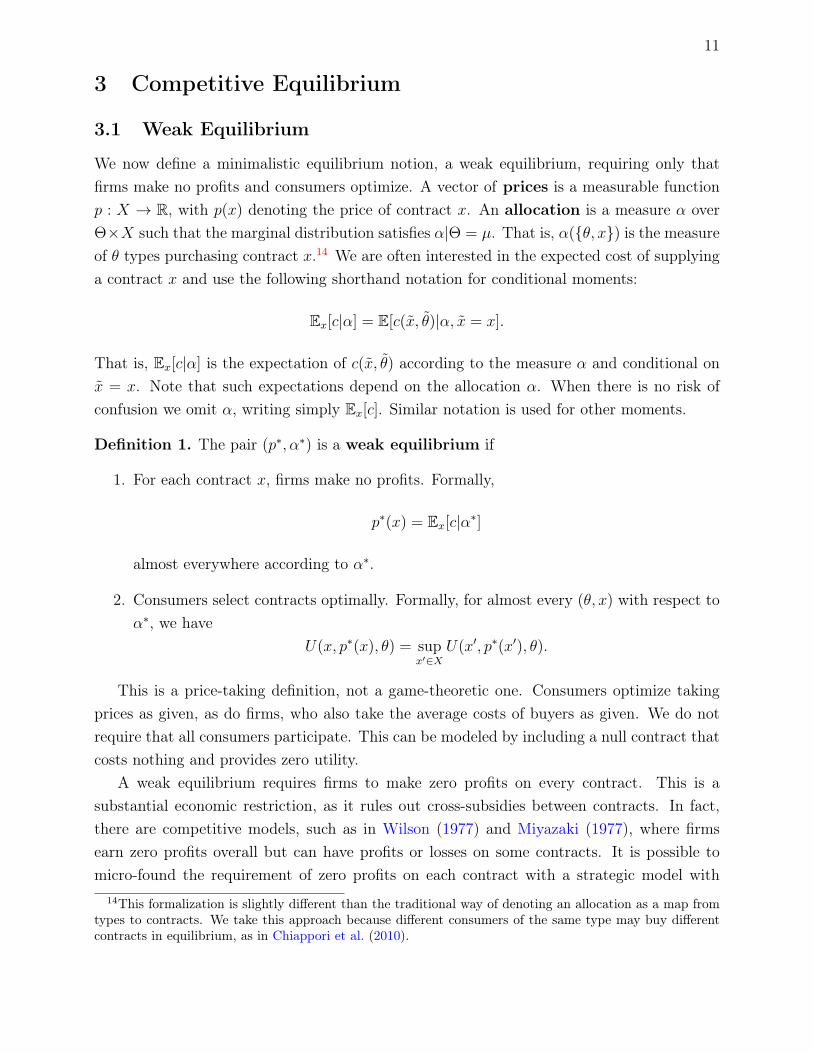
3 Competitive Equilibrium

3.1 Weak Equilibrium

We now define a minimalistic equilibrium notion, a weak equilibrium, requiring only thatfirms make no profits and consumers optimize. A vector of prices is a measurable functionp : X → R, with p(x) denoting the price of contract x. An allocation is a measure α overΘ×X such that the marginal distribution satisfies α|Θ = µ. That is, α({θ, x}) is the measureof θ types purchasing contract x.14 We are often interested in the expected cost of supplyinga contract x and use the following shorthand notation for conditional moments:

Ex[c|α] = E[c(x̃, θ̃)|α, x̃ = x].

That is, Ex[c|α] is the expectation of c(x̃, θ̃) according to the measure α and conditional onx̃ = x. Note that such expectations depend on the allocation α. When there is no risk ofconfusion we omit α, writing simply Ex[c]. Similar notation is used for other moments.

Definition 1. The pair (p∗, α∗) is a weak equilibrium if

1. For each contract x, firms make no profits. Formally,

p∗(x) = Ex[c|α∗]

almost everywhere according to α∗.

2. Consumers select contracts optimally. Formally, for almost every (θ, x) with respect toα∗, we have

U(x, p∗(x), θ) = supx′∈X

U(x′, p∗(x′), θ).

This is a price-taking definition, not a game-theoretic one. Consumers optimize takingprices as given, as do firms, who also take the average costs of buyers as given. We do notrequire that all consumers participate. This can be modeled by including a null contract thatcosts nothing and provides zero utility.

A weak equilibrium requires firms to make zero profits on every contract. This is asubstantial economic restriction, as it rules out cross-subsidies between contracts. In fact,there are competitive models, such as in Wilson (1977) and Miyazaki (1977), where firmsearn zero profits overall but can have profits or losses on some contracts. It is possible tomicro-found the requirement of zero profits on each contract with a strategic model with

14This formalization is slightly different than the traditional way of denoting an allocation as a map fromtypes to contracts. We take this approach because different consumers of the same type may buy differentcontracts in equilibrium, as in Chiappori et al. (2010).

12

differentiated products, as discussed in Section 4.2. Intuitively, in this kind of model, a firmthat tries to cross-subsidize contracts is undercut in contracts that it taxes and is left sellingthe contracts that it subsidizes.

We only ask that prices equal expected costs almost everywhere.15 In particular, weakequilibria place no restrictions on the prices of contracts that are not purchased. As demon-strated in the examples below, this is a serious problem with this definition and the reasonwhy a stronger equilibrium notion is necessary.

3.2 Equilibrium Multiplicity and Free Entry

We now illustrate that weak equilibria are compatible with a wide variety of outcomes, mostof which are unreasonable in a competitive marketplace.

Example 2′. (Rothschild and Stiglitz - Multiplicity of Weak Equilibria) We first revisitRothschild and Stiglitz’s (1976) original equilibrium. They set up a Bertrand game withidentical firms and showed that, when a Nash equilibrium exists, it has allocations givenby the points L and H in Figure 2b. High-risk consumers buy full insurance xH = 1 atactuarially fair rates pH = H · l. Low-risk types purchase partial insurance, with actuariallyfair prices reflecting their lower risk. The level of coverage xL is just low enough so thathigh-risk consumers do not wish to purchase contract xL. That is, L and H are on the sameindifference curve ICH of high types.

Note that we can find weak equilibria with the same allocation. One example of weakequilibrium prices is the curve p(x) is Figure 2b. The zero profits condition is satisfiedbecause the prices of the two contracts that are traded, xL and xH , equal the average cost ofproviding them. The optimization condition is also satisfied because the price schedule p(x)

is above the indifference curves ICL and ICH . Therefore, no consumer wishes to purchase adifferent bundle.

However, many other weak equilibria exist. One example is the same allocation with theprices p̃(x) in Figure 2b. Again, firms make no profits because the prices of xH and xL areactuarially fair, and consumers are optimizing because the price of other contracts is higherthan their indifference curves.

There are also weak equilibria with completely different allocations. For example, it isa weak equilibrium for all consumers to purchase full insurance, and for all other contractsto be priced so high that no one wishes to buy them. This does not violate the zero profitscondition because the expected cost of contracts that are not traded is arbitrary. This weakequilibrium has full insurance, which is the first-best outcome in this model. It is also a weak

15The reason is that conditional expectation is only defined almost everywhere. Although it is possible tounderstand all of our substantive results without recourse to measure theory, we refer interested readers toBillingsley (2008) for a formal definition of conditional expectation.

13

equilibrium for no insurance to be sold, and for prices of all contracts with positive coverageto be prohibitively high. Therefore, weak equilibria provide very coarse predictions, with theBertrand solution, full insurance, complete unraveling, and many other outcomes all beingpossible.

In a market with free entry, however, some weak equilibria are more reasonable thanothers. Consider the case of H < 1 and take the weak equilibrium with complete unravelling.Suppose firms enter the market for a policy with positive coverage, driving down its price.Initially no consumers purchase the policy, and firms continue to break even. As pricesdecrease enough to reach the indifference curve of high-risk consumers, they start buying. Atthis point, firms make money because risk averse consumers are willing to pay a premium forinsurance. Therefore, this weak equilibrium conflicts with the idea of free entry. A similartâtonnement eliminates the full-insurance weak equilibrium. If firms enter the market forpartial insurance policies, driving down prices, they do not attract any consumers at first.However, once prices decrease enough to reach the indifference curve of low-risk consumers,firms only attract good risks and therefore make positive profits.

The same argument eliminates the weak equilibrium associated with p̃(x). Let x0 < xL

be a non-traded contract with p̃(x0) > p(x). Suppose firms enter the market for x0, drivingdown its price. Initially no consumers purchase x0, and firms continue to break even. Asprices decrease enough to reach p(x0), the L types become indifferent between purchasing x0or not. If they decrease any further, all L types purchase contract x0. At this point, firmslose money because average cost is higher than the price.16 The price of x0 is driven down top(x0), at which point it is no longer advantageous for firms to enter. In fact, this argumenteliminates all but the weak equilibrium with price p(x) and the allocation in Figure 2b.

3.3 Definition and Existence of an Equilibrium

We now define an equilibrium concept that formalizes the free entry argument. Equilibriaare required to be robust to small perturbations of a given economy. A perturbation has alarge but finite set of contracts approximating X. The perturbation adds a small measureof behavioral types, who always purchase each of the existing contracts and impose no costson firms. The point of considering perturbations is that all contracts are traded, eliminatingthe paradoxes associated with defining the average cost of non-traded contracts.

We introduce, for each contract x, a behavioral consumer type who always demandscontract x. We write x for such a behavioral type and extend the utility and cost functionsas U(x, p, x) = ∞, U(x′, p, x) = 0 if x′ 6= x, and c(x, x) = 0. For clarity, we refer tonon-behavioral types as standard types.

16To see why, note that L types buy xL at an actuarially fair price. Therefore, they would only purchaseless insurance if firms sold it at a loss.

14

Definition 2. Consider an economy E = [Θ, X, µ]. A perturbation of E is an economywith a finite set of contracts X̄ ⊆ X and a small mass of behavioral types demanding eachcontract in X̄. Formally, a perturbation (E, X̄, η) is an economy [Θ ∪ X̄, X̄, µ + η], whereX̄ ⊆ X is a finite set, and η is a strictly positive measure over X̄.17

The next definition says that a sequence of perturbations converges to the original econ-omy if the set of contracts fills in the original set of contracts and the total mass of behavioralconsumers converges to 0.

Definition 3. A sequence of perturbations (E, X̄n, ηn)n∈N converges to E if

1. Every point in X is the limit of a sequence (xn)n∈N with each xn ∈ X̄n.

2. The total mass of behavioral types ηn(X̄n) converges to 0.

We now define what it means for a sequence of equilibria of perturbations to converge tothe original economy.

Definition 4. Take an economy E and a sequence of perturbations (E, X̄n, ηn)n∈N converg-ing to E, with weak equilibria (pn, αn). The sequence of weak equilibria (pn, αn)n∈N

converges to a price-allocation pair (p∗, α∗) of E if

1. The allocations αn converge weakly to α∗.

2. For every sequence (xn)n∈N with each xn ∈ X̄n and limit x ∈ X, pn(xn) converges top∗(x).18

We are now ready to define an equilibrium.

Definition 5. The pair (p∗, α∗) is an equilibrium of E if there exists a sequence of pertur-bations that converges to E and an associated sequence of weak equilibria that converges to(p∗, α∗).

The most transparent way to understand how equilibrium formalizes the free entry ideais to return to the Rothschild and Stiglitz model from example 2. Recall that there is aweak equilibrium where no one purchases insurance and prices are high. But this is notan equilibrium. A perturbation cannot have such high-price equilibria because, if standard

17Both an economy and its perturbations have a set of types contained in Θ ∪X and contracts containedin X. To save on notation, we extend distributions of types to be defined over Θ ∪X and allocations to bedefined over (Θ∪X)×X. With this notation, measures pertaining to different perturbations are defined onthe same space.

18In a perturbation, prices are only defined for a finite subset X̄n of contracts. The definition of convergenceis strict in the sense that, for a given contract x, prices must converge to the price of x for any sequence ofcontracts (xn)n∈N converging to x.

15

types do not purchase insurance, prices are driven to 0 by behavioral types. Likewise, theweak equilibrium corresponding to p̃ in Figure 2b is not an equilibrium. Consider a contractx0 with p̃(x0) > p(x0). In any perturbation, if prices are close to p̃, then only behavioraltypes would buy x0. But this would make the price of x0 equal to 0 because the only way tosustain positive prices in a perturbation is by attracting standard types. In fact, equilibria ofperturbations sufficiently close to E involve most L types purchasing contracts similar to xL,and mostH types purchasing contracts similar to xH . The price of any contract x0 < xL mustmake L types indifferent between x0 and xL. There is a small mass of L types purchasingx0 to maintain the indifference. If prices were lower, L types would flood the market for x0,and firms would lose money. If prices were higher, no L types would purchase x0. The onlyequilibrium is that corresponding to p(x) in Figure 2b (this is proven in Corollary 1).

The mechanics of equilibrium are similar to the standard analysis of the Akerlof modelfrom example 1. In the example depicted in Figure 2a, the only equilibrium is that associatedwith the intersection of demand and average cost.19 This is similar to the way that pricesfor xL and xH are determined in example 2. If the average cost curve were always above thedemand curve, the only equilibrium would be complete unraveling. This is analogous to theway that the market for contracts other than xL and xH unravels.

There are two ways to think about the equilibrium requirement. One is that it consistentlyapplies the logic of Akerlof (1970) and Einav et al. (2010a) to the case where there is more thanone potential contract. This is similar to the intuitive free entry argument discussed in Section3.2. Another interpretation is that the definition demands a minimal degree of robustnesswith respect to perturbations, while paradoxes associated with conditional expectation donot occur in perturbations. This rationale is similar to proper equilibria (Myerson, 1978).

We now show that equilibria always exist.

Theorem 1. Every economy has an equilibrium.

The proof is based on two observations. First, equilibria of perturbations exist by astandard fixed-point argument. Second, equilibrium price schedules in any perturbation areuniformly Lipschitz. This is a consequence of the bounded marginal rate of substitution(Assumption 2). The intuition is that, if prices increased too fast with x, no standard typeswould be willing to purchase more expensive contracts. This is impossible, however, because acontract cannot have a high equilibrium price if it is only purchased by the low-cost behavioraltypes. We then apply the Arzelà–Ascoli Theorem to demonstrate existence of equilibria.

19There are other weak equilibria in the example in Figure 2a, but the only equilibrium is the intersectionbetween demand and average cost. For example, it is a weak equilibrium for no one to purchase insurance,and for prices to be very high. But this is not an equilibrium. The reason is that, in a perturbation, behavioraltypes make the average cost curve well-defined for all quantities, including 0. The perturbed average costcurve is continuous, equal to 0 at a quantity of 0, and slightly lower than the original. As the mass ofbehavioral types shrinks, the perturbed average cost curve approaches its value in the original economy.Consequently, the only equilibrium is the standard solution, where demand and average cost intersect.

16

0 0.2 0.4 0.6 0.8 1$0

$2,000

$4,000

$6,000

$8,000

Contract

($)

Equilibrium PricesAverage Loss Parameter

(a)

$1,000 $10,000 $100,00010

−6

10−5

10−4

Average Loss, Mθ

Ris

k A

vers

ion, A

θ

0.2

0.4

0.6

0.8

1

(b)

Figure 3: Equilibrium prices (a) and demand profile (b) in the multidimensional healthinsurance model from example 3.

Notes: Panel (a) illustrates equilibrium prices and quantities in example 3 under benchmark parameters.The solid curve denotes prices. The size of the circles represent the mass of consumers purchasing eachcontract, and its height represents the average loss parameter of such consumers, that is Ex[M ]. Panel (b)illustrates the equilibrium demand profile. Each point represents a randomly drawn type from the population.The horizontal axis represents expected health shock Mθ, and the vertical axis represents the absolute riskaversion coefficient Aθ. The colors represent the level of coverage purchased in equilibrium.

Existence only depends on the assumptions of Section 2.3. Therefore, equilibria are well-defined in a broad range of theoretical and empirical models. Equilibria exist not only instylized models, but also in rich multidimensional settings. Figure 3 plots an equilibrium ina calibration of the Einav et al. model (example 3). Equilibrium makes sharp predictions,displays adverse selection, with costlier consumers purchasing higher coverage, and consumerssort across the four dimensions of private information. We return to this example below.

4 Discussion

This section establishes consequences of competitive equilibrium, and discusses the relation-ship to existing solution concepts.

4.1 Equilibrium Properties

We begin by describing some properties of equilibria.

Proposition 1. Let (p∗, α∗) be an equilibrium of economy E. Then:

1. The pair (p∗, α∗) is a weak equilibrium of E.

17

2. For every contract x′ ∈ X with strictly positive price, there exists (θ, x) in the supportof α∗ such that

U(x, p∗(x), θ) = U(x′, p∗(x′), θ) and c(x′, θ) ≥ p(x′).

That is, every contract that is not traded in equilibrium has a low enough price for someconsumer to be indifferent between buying it or not, and the cost of this consumer is atleast as high as the price.

3. The price function is L-Lipschitz, and, in particular, continuous.

4. If X is a subset of Euclidean space, then p∗ is Lebesgue almost everywhere differentiable.

The proposition shows that equilibria have several regularity properties. They are weakequilibria. Moreover, equilibrium prices are continuous and differentiable almost everywhere.Finally, the price of an out-of-equilibrium contract is either 0, or low enough that some typeis indifferent between buying it or not. Moreover, the cost of selling to this indifferent type isat least as high as the price. Intuitively, these are the consumer types who make the marketfor this contract unravel.20

With these properties, we can solve for equilibria in the Rothschild and Stiglitz model:

Corollary 1. Consider example 2. If H < 1, the unique equilibrium is the price p andallocation in Figure 2b. If H = 1, the market unravels with equilibrium prices of x · l and lowtypes purchasing no insurance.

The corollary shows that equilibrium coincides with the Riley (1979) equilibrium and withthe Rothschild and Stiglitz (1976) equilibrium when it exists.21 Therefore, competitive equi-librium delivers the standard results in the particular cases of Akerlof (1970) and Rothschild

20These conditions are necessary but not sufficient for an equilibrium. The reason is that the existence ofa type satisfying the conditions in Part 2 of the proposition does not imply that the market for a contractx would unravel in a perturbation. This may happen because there can be other types who are indifferentbetween purchasing x or not, and some of them may have lower costs. It is simple to construct these examplesin models similar to Chang (2010) or Guerrieri and Shimer (2013).

21There is some controversy in the literature on whether the Riley (1979) equilibrium is reasonable (andwhether other notions, such as the Wilson (1977) equilibrium, are more compelling). The Riley allocation hasbeen criticized because it is constrained inefficient when there are few H types (Crocker and Snow, 1985a),and because the equilibrium does not depend on the proportion of each type and changes discontinuously tofull insurance when the measure of H types is 0 (Mailath et al., 1993). Although our solution concept inheritsthese counter-intuitive predictions, we see it as reasonable, especially in the richer settings in which we areinterested, for two reasons. First, the Rothschild and Stiglitz assumptions are extreme and counter-intuitive,with consumers having only two types and being heterogeneous across a single dimension. Thus, the counter-intuitive results are driven not only by the equilibrium concept but also by counter-intuitive assumptions.We also give some evidence that the Rothschild and Stiglitz setting is atypical in Appendix D. The appendixshows that, under certain assumptions, generically, the set of competitive equilibria varies continuously withfundamentals. Moreover, whenever there is some pooling (as in example 3) , the equilibrium will depend onthe distribution of types. Second, our model produces intuitive predictions and comparative statics in our

18

and Stiglitz (1976). Moreover, simple arguments based on Proposition 1 can be used to solvemodels with richer heterogeneity, such as Netzer and Scheuer (2010), where the analysis ofgame-theoretic solution concepts is challenging.

4.2 Strategic Foundations

Our equilibrium concept can be justified as the limit of a strategic model, which is similar tothe models used in the empirical industrial organization literature. This relates our work tothe literature on game-theoretic competitive screening models and the industrial organizationliterature on adverse selection. Moreover, the assumptions on the strategic game clarify thelimitations of our model and the situations where competitive equilibrium is a reasonableprediction.

We consider such a strategic setting in Appendix B. We start from a perturbation(E, X̄, η). Each contract has n differentiated varieties, and each variety is sold by a differentfirm. Consumers have logit demand with semi-elasticity σ. Firms have a small efficient scale.To capture this in a simple way, we assume that each firm can only serve up to a fraction kof consumers. Firms cannot turn away consumers, as with community rating regulations.22

The key parameters are the number of varieties of each contract n, the semi-elasticity ofdemand σ, and the maximum scale of each firm k.

We consider symmetric Bertrand-Nash equilibria, where firms independently set prices.Proposition B1 shows that Bertrand-Nash equilibria exist as long as firm scale is sufficientlysmall and there are enough firms selling each product to serve the whole market. Themaximum scale that guarantees existence is of the order of the inverse of the semi-elasticity.Therefore, equilibria exist even if demand is close to the limit of no differentiation. At afirst blush, this result seems to contradict the finding that the Rothschild and Stiglitz modeloften has no Nash equilibrium (Riley, 1979). The reason why Bertrand-Nash equilibria existis that the profitable deviations in the Rothschild and Stiglitz model rely on firms settingvery low prices and attracting a sizable portion of the market. However, this is not possibleif firms have small scale and cannot turn consumers away. Besides establishing existence ofa Bertrand-Nash equilibrium, Proposition B1 shows that profits per contract are bounded

application in Section 5. While we see our framework as a reasonable first step to study markets with richconsumer heterogeneity, it would be interesting to explore alternative equilibrium notions in settings withrich heterogeneity. For example, it would be interesting to generalize the Wilson (1977) equilibrium to suchsettings. Moreover, we caution readers that, while we seek to propose a useful framework that can be appliedmore generally, we do not seek to resolve the debate about whether the Riley (1979) or the Wilson (1977)concept is more appropriate in the Rothschild and Stiglitz example. Nevertheless, we believe that exploringalternative equilibrium notions in settings with more realistic assumptions on preferences can contribute tounderstanding what equilibrium notions produce useful predictions in these settings.

22Instead of assuming a small efficient scale, we could establish similar results by requiring that strategiesare only locally optimal. See Appendix B.3.

19

above by a term of order 1/σ plus a term of order k.Proposition B2 then shows that, for a sequence of parameters satisfying the conditions for

existence and with semi-elasticity converging to infinity, Bertrand-Nash equilibria convergeto a competitive equilibrium. Thus, competitive equilibrium corresponds to the limit of thisgame-theoretic model.

A limitation of this result is that each firm offers a single contract, as opposed to a menuof contracts. In particular, the strategic model rules out the possibility that firms cross-subsidize contracts, which is a key requirement of our equilibrium notion. To address this,we generalize our convergence results to the case where firms offer menus of contracts inAppendix C. This generalization shows that, even if firms can cross-subsidize contracts, inequilibrium they do not do so, and earn low profits on all contracts.

These results have four implications. First, convergence to competitive equilibrium isrelatively brittle because it depends on the Bertrand assumption, on the number of varietiesand maximum scale satisfying a pair of inequalities, and on semi-elasticities growing at a fastenough rate relative to those parameters. This is to be expected because existing strategicmodels lead to very different conclusions with small changes in assumptions. Second, althoughconvergence depends on special assumptions, it is not a knife-edge case. There exists a non-trivial set of parameters for which equilibria are justified by a strategic model.

Third, our results relate two types of models in the literature. Our strategic model isclosely related to the differentiated products models in the industrial organization literature,such as Starc (2014), Decarolis et al. (2012), Mahoney and Weyl (2014), and Tebaldi (2015).Our results show that our competitive equilibrium corresponds to a particular limiting caseof these models. This implies that the models of Riley (1979) and Handel et al. (2015) arealso limiting cases of the differentiated products models, because their equilibria coincidewith ours in particular cases, as dicussed below.

Finally, the sufficient conditions give insight into situations where competitive equilibriumis reasonable. Namely, when there are many firms, efficient firm scale is small relative to themarket, and firms are close to undifferentiated. The results do not imply that markets withadverse selection are always close to perfect competition. Indeed, market power is often anissue in these markets (see Dafny, 2010, Dafny et al., 2012, and Starc, 2014). Nevertheless, thesufficient conditions are similar to those in markets without adverse selection: the presenceof many, undifferentiated firms, with small scale relative to the market (see Novshek andSonnenschein, 1987).

4.3 Unravelling and Robustness to Changes in Fundamentals

It is possible that there is no trade in one or all competitive equilibria. This is illustratedin Corollary 1 and in other particular cases of our model. For example, with one contract

20

(example 1), there is no trade if average cost is always above the demand curve, as in Akerlof’sclassic example. Hendren (2013) gives a no-trade condition in a binary loss model with aricher contract space.

Unravelling examples such as those in Hendren (2013) raise the question of whethercompetitive equilibria are too sensitive to small changes in fundamentals. For example,consider an Akerlof model as in example 1, with a unique equilibrium, which has a positivequantity. Suppose we add a positive but small mass of a type who values every non-nullcontract more than all other types, say $1,000,000, and has even higher costs, say $2,000,000.This change in fundamentals creates a new equilibrium where all contracts cost $1,000,000and no contracts are traded (although there may be other equilibria close to the originalone).

Appendix D examines the robustness of the set of equilibria with respect to fundamentals.We give examples in the one-contract case where adding a small mass of high-cost typesintroduces a new equilibrium with complete unraveling. However, competitive equilibriahave two important generic robustness properties. First, generically, equilibria with trade arenever considerably affected by the introduction of a small measure of high-cost types. Second,generically, small changes to demand and average cost curves lead to small changes in theset of equilibria. That is, the only way to produce large changes in equilibrium predictions isto considerably move average cost or demand curves. In particular, the $1,000,000 exampleonly works because it considerably changes expected costs conditioning on the consumerswho have sufficiently high willingness to pay. This would not be possible if, for example,the original model already had consumers with high willingness to pay. Finally, Appendix Dgives a formal result showing that the latter robustness property holds with many potentialcontracts.

4.4 Equilibrium Multiplicity and Pareto Ranked Equilibria

Competitive equilibria may not be unique. This is the case, for example, in the Akerlofmodel (Example 1) when average cost and demand cross at multiple points. This exampleis counterintuitive because equilibria are Pareto ranked, so market participants may attemptto coordinate on the Pareto superior equilibrium. Moreover, only the lowest-price crossing ofaverage cost and demand is an equilibrium under the standard strategic equilibrium conceptin Einav et al. (2010a). Thus, in applications, a researcher may choose to select Paretodominant equilibria, as commonly done in dynamic oligopoly models and cheap talk games.

While this selection is sometimes compelling, we note that multiple equilibria are a stan-dard feature of Walrasian models. There is experimental evidence that multiple equilibria areobserved in competitive markets where supply is downward sloping (Plott and George, 1992).In markets with adverse selection, Wilson (1980) pointed out the potential multiplicity of

21

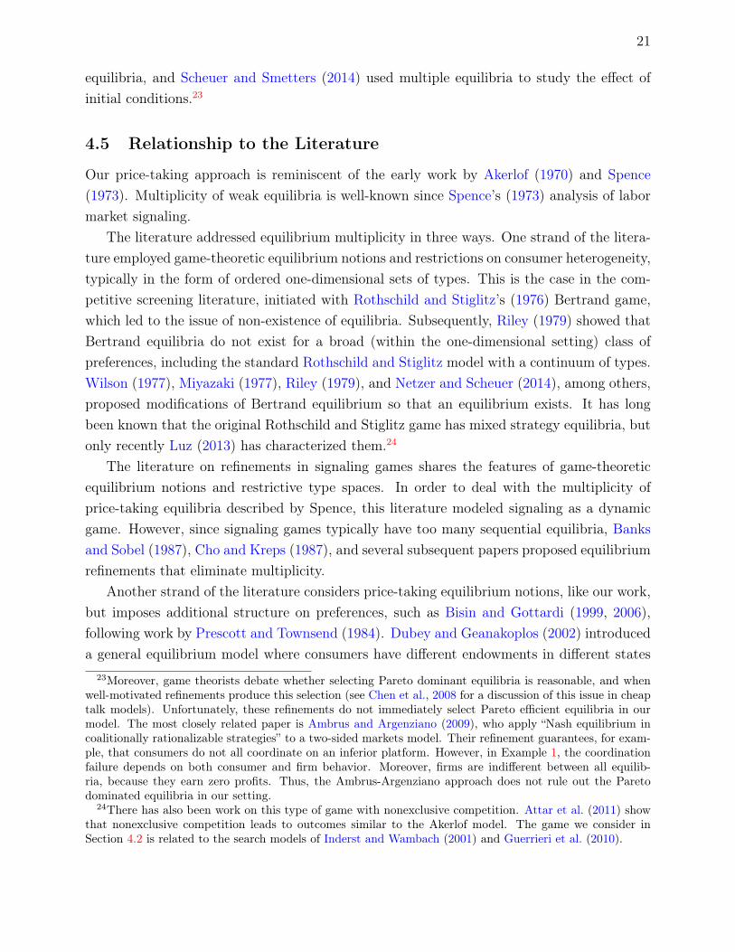
equilibria, and Scheuer and Smetters (2014) used multiple equilibria to study the effect ofinitial conditions.23

4.5 Relationship to the Literature

Our price-taking approach is reminiscent of the early work by Akerlof (1970) and Spence(1973). Multiplicity of weak equilibria is well-known since Spence’s (1973) analysis of labormarket signaling.

The literature addressed equilibrium multiplicity in three ways. One strand of the litera-ture employed game-theoretic equilibrium notions and restrictions on consumer heterogeneity,typically in the form of ordered one-dimensional sets of types. This is the case in the com-petitive screening literature, initiated with Rothschild and Stiglitz’s (1976) Bertrand game,which led to the issue of non-existence of equilibria. Subsequently, Riley (1979) showed thatBertrand equilibria do not exist for a broad (within the one-dimensional setting) class ofpreferences, including the standard Rothschild and Stiglitz model with a continuum of types.Wilson (1977), Miyazaki (1977), Riley (1979), and Netzer and Scheuer (2014), among others,proposed modifications of Bertrand equilibrium so that an equilibrium exists. It has longbeen known that the original Rothschild and Stiglitz game has mixed strategy equilibria, butonly recently Luz (2013) has characterized them.24

The literature on refinements in signaling games shares the features of game-theoreticequilibrium notions and restrictive type spaces. In order to deal with the multiplicity ofprice-taking equilibria described by Spence, this literature modeled signaling as a dynamicgame. However, since signaling games typically have too many sequential equilibria, Banksand Sobel (1987), Cho and Kreps (1987), and several subsequent papers proposed equilibriumrefinements that eliminate multiplicity.

Another strand of the literature considers price-taking equilibrium notions, like our work,but imposes additional structure on preferences, such as Bisin and Gottardi (1999, 2006),following work by Prescott and Townsend (1984). Dubey and Geanakoplos (2002) introduceda general equilibrium model where consumers have different endowments in different states

23Moreover, game theorists debate whether selecting Pareto dominant equilibria is reasonable, and whenwell-motivated refinements produce this selection (see Chen et al., 2008 for a discussion of this issue in cheaptalk models). Unfortunately, these refinements do not immediately select Pareto efficient equilibria in ourmodel. The most closely related paper is Ambrus and Argenziano (2009), who apply “Nash equilibrium incoalitionally rationalizable strategies” to a two-sided markets model. Their refinement guarantees, for exam-ple, that consumers do not all coordinate on an inferior platform. However, in Example 1, the coordinationfailure depends on both consumer and firm behavior. Moreover, firms are indifferent between all equilib-ria, because they earn zero profits. Thus, the Ambrus-Argenziano approach does not rule out the Paretodominated equilibria in our setting.

24There has also been work on this type of game with nonexclusive competition. Attar et al. (2011) showthat nonexclusive competition leads to outcomes similar to the Akerlof model. The game we consider inSection 4.2 is related to the search models of Inderst and Wambach (2001) and Guerrieri et al. (2010).

22

of the world, and may join “competitive pools” to share risk. They write the Rothschildand Stiglitz setup as a particular case. Dubey et al. (2005) considered a related modelwith endogenous default and non-exclusive contracts. These papers address multiplicity ofequilibria with a refinement where an “external agent” makes high deliveries to each pool inevery state of the world. This refinement is similar to our approach in the case of a finitenumber of contracts. There are three main differences with respect to our work. First, weconsider more general preferences, that can accommodate richer preference heterogeneity in asimple way as in example 3. Second we allow for continuous sets of contracts, as in examples2 and 3. To do so, we generalize the equilibrium refinement, make the key assumptionof bounded marginal rates of substitution, and develop the proof strategy of Theorem 1.Third, we introduce new analytical techniques by analyzing our examples directly in thelimit, enabling novel applied results such as Propositions 2 and 3.

Gale (1992), like us, considers general equilibrium in a setting with less structure than theinsurance pools. However, he refines his equilibrium with a stability notion based on Kohlbergand Mertens (1986). More recent contributions have considered general equilibrium modelswhere firms can sell the right to choose from menus of contracts (Citanna and Siconolfi,2014).

Our results are related to this previous work as follows. In standard one-dimensionalmodels with ordered types, our unique equilibrium corresponds to what is usually calledthe “least-costly separating equilibrium.” Thus, our equilibrium prediction is the same asin models without cross-subsidies, such as Riley (1979), Bisin and Gottardi (2006), andRothschild and Stiglitz (1976) when their equilibrium exists. It also coincides with Banksand Sobel (1987) and Cho and Kreps (1987) in the settings they consider. It differs fromequilibria that involve cross-subsidization across contracts, such as Wilson (1977), Miyazaki(1977), Hellwig (1987), and Netzer and Scheuer (2014). Our equilibrium differs from mixedstrategy equilibria of the Rothschild and Stiglitz (1976) model, even as the number of firmsincreases. This follows from the Luz (2013) characterization. In the case of a pool structureand finite set of contracts, our equilibria are the same as in Dubey and Geanakoplos (2002).

Although our equilibrium coincides with the Riley equilibrium in particular settings, ourequilibrium exists, is tractable, and has strategic foundations in settings where the Rileyequilibrium may not exist. Our predictions are the same as the Riley equilibrium in twoimportant particular cases. One is Riley’s (1979) original setup with ordered types, and theother is Handel et al.’s (2015) model, where types come from a more realistic empirical healthinsurance model and are not ordered, but there are only two contracts. In particular, ourstrategic foundations results lend support to the predictions in these models. We note that,with multidimensional heterogeneity, existence of Riley equilibrium can only be guaranteedwith restrictions on preferences (see Azevedo and Gottlieb, 2016 for a simple example where

23

a Riley equilibrium does not exist).Another strand of the literature considers preferences with less structure. Chiappori et al.

(2006) consider a very general model of preferences within an insurance setting. This paperdiffers from our work in that they consider general testable predictions without specifyingan equilibrium concept, while we derive sharp predictions within an equilibrium framework.Rochet and Stole (2002) consider a competitive screening model with firms differentiated as inHotelling (1929), where there is no adverse selection. Their Bertrand equilibrium converges tocompetitive pricing as differentiation vanishes, which is the outcome of our model. However,Riley’s (1979) results imply that no Bertrand equilibrium would exist if one generalizes theirmodel to include adverse selection.

Veiga and Weyl (2014b) and Handel et al. (2015) consider endogenous contract charac-teristics in a multidimensional framework. Handel et al. (2015) develop a tractable modelby using Riley equilibria with a simple set of contracts. Veiga and Weyl (2014b) consideran oligopoly model of competitive screening in the spirit of Rochet and Stole (2002), butwhere each firm offers a single contract. Contract characteristics are determined by a simplefirst-order condition, as in the Spence (1975) model. Moreover, their model can incorporateimperfect competition. Our numerical results suggest that the our model and Veiga andWeyl’s agree on many qualitative predictions. For example, insurance markets provide ineffi-ciently low coverage, and increasing heterogeneity in risk aversion seems to attenuate adverseselection.

The key difference is that their model has a single traded contract, while our modelendogenously determines the set of traded contracts. In their model, when competitiveequilibria exist,25 all firms offer the same contract.26 In contrast, a rich set of contracts isoffered in our equilibrium. For example, in the case of no adverse selection (when costs areindependent of types), our equilibrium is for firms to offer all products priced at cost, whichcorresponds to the standard notion of perfect competition. A colorful illustration is tomatosauce. The Veiga and Weyl (2014b) model predicts that a single type of tomato sauce isoffered cheaply, with characteristics determined by the preferences of average consumers. Incontrast, our prediction is that many different types of tomato sauce are sold at cost. Italianstyle, basil, garlic lover, chunky, mushroom, and so on. In a less gastronomically titillatingexample, insurers offer a myriad types of life insurance: term life, universal life, whole life,combinations of these categories, and many different parameters within each category. Ourresults on the convergence of Bertrand equilibria suggest that the two models are appropriatein different situations. Their model of perfect competition seems more relevant when there are

25Perfectly competitive equilibria do not always exist in their model. In a calibration they find thatperfectly competitive symmetric equilibria do not exist, and equilibria only exist with very high markups.

26This is so in the more tractable case of symmetrically differentiated firms. In general, the number ofcontracts offered is no greater than the number of firms.

24

few firms, which are not very differentiated, the fixed cost of creating a new contract is high,and it is a good strategy for firms to offer products of similar quality as their competitors.That is, when firms herd on a particular type of contract.

5 Application: Equilibrium Effects of Mandates

5.1 Calibration

We calibrated the multidimensional health insurance model from example 3 to illustrate theequilibrium concept and understand equilibrium effects of policy interventions. To under-stand what effects are quantitatively plausible, we calibrated the model based on Einav etal.’s (2013) preference estimates from employees in a large US corporation.27

We considered linear contracts and normal losses. The advantage of this parametricrestriction is that willingness to pay and costs are transparently represented by equation(2). Consumers differ along four dimensions: expected health shock, standard deviationof health shocks, moral hazard, and risk aversion. All parameters are readily interpretablefrom equation (2). We assumed that the distribution of parameters in the population is log-normal.28 Moments of the type distribution were calibrated to match the central estimates ofEinav et al. (2013), as in Table 1. There are two exceptions. We reduced average risk aversionbecause linear contracts involve losses in a much wider range than the contracts in their data.Lower risk aversion better matched the substitution patterns in the data because constantabsolute risk aversion models do not work well across different ranges of losses (Rabin, 2000and Handel and Kolstad, forthcoming). The other exception is the log variance of moralhazard, which we vary in our simulations. In our baseline we set σ2

H to 0.28. See AppendixE for details on the calibration and computational procedures. Appendix F shows that thekey qualitative results hold with nonlinear contracts similar to those typically used in healthinsurance markets and to those in Einav et al. (2013).

To calculate an equilibrium, we used a perturbation with 26 evenly spaced contracts,and added a mass equal to 1% of the population as behavioral consumers. We then used afixed-point algorithm. In each iteration, consumers choose optimal contracts taking prices asgiven. Prices are adjusted up for unprofitable contracts and down for profitable contracts.Prices consistently converge to the same equilibrium for different initial values.

The equilibrium is depicted in Figure 3a. It features adverse selection with respect to27Our simulations are not aimed at predicting the outcomes in a particular market as in Aizawa and Fang

(2013) and Handel et al. (2015). Such simulations would take the Einav et al. (2013) estimates far outsidethe range of contracts in their data, so even predictions about demand would rely heavily on functional formrestrictions.

28Note that the set of types is not compact in our numerical simulations. Restricting the set of types to alarge compact set does not meaningfully impact the numerical results.

25

Table 1: Calibrated distribution of consumer types

A H M SMean 1.0E-5 1,330 4,340 24,474

Log covarianceA 0.25 -0.01 -0.12 0H σ2

logH -0.03 0M 0.20 0S 0.25

Notes: In all simulations of the health insurance example, consumer types are log normally distributed withthe moments in the table.

0 0.2 0.4 0.6 0.8 1$0

$2,000

$4,000

$6,000

$8,000

Contract

($)

No Mandate − PricesNo Mandate − LossesMandate − PricesMandate − Losses

(a)

0 0.2 0.4 0.6 0.8 1$0

$2,000

$4,000

$6,000

$8,000

Contract

($)

Equilibrium PricesEquilibrium LossesOptimum PricesOptimum Losses

(b)

Figure 4: Equilibrium prices with a 60% mandate (a) and optimal prices (b).

Notes: The graphs plot equilibria of the multidimensional health insurance model from example 3. In bothgraphs, the solid curve denotes prices. The size of the circles represent the mass of consumers purchasingeach contract, and its height represents the average loss parameter of such consumers, that is Ex[M ].

the average loss, in the sense that, on average, consumers who purchase more coverage havehigher losses. Moreover, consumers sort across contracts in accordance to their preferences.This is illustrated in Figure 3b, which displays the contracts purchased by consumers withdifferent expected loss and risk aversion parameters. The figure corroborates the existenceof adverse selection on average loss, as consumers with higher expected losses tend to choosemore generous contracts. However, even for the same levels of risk aversion and expectedloss, different consumers choose different contracts due to other dimensions of heterogeneity.

Although there is adverse selection, equilibria do not feature a complete “death spiral,”where no contracts are sold. It is also possible that the support of traded contracts is a smallsubset of all contracts. Whenever this is the case, buyers with the highest willingness to payfor each contract that is not traded value it below their own average cost (Proposition 1).That is, the markets for non-traded contracts are shut down by an Akerlof-type death spiral.

26

5.2 Policy Interventions

This section investigates the effects of policy interventions. We focus on a mandate requiringconsumers to purchase at least 60% coverage. Equilibrium is depicted in Figures 1 and4a. With the mandate, about 85% of consumers get the minimum coverage. Moreover, someconsumers who originally chose policies with greater coverage switch to the minimum amountafter the mandate. In fact, the mandate increases the fraction of consumers who buy 60%coverage or less, as only 80% of consumers did so before the mandate.

The reason why some consumers reduce their coverage is that the mandate exacerbatesadverse selection on the intensive margin. With the mandate, many low-cost consumers pur-chase the minimum coverage. This reduces the price of the 60% policy, attracting consumerswho were originally purchasing more generous policies. In equilibrium, consumers sort acrosspolicies so that prices are continuous (as must be the case by Proposition 1). This leads toa lower but steeper price schedule, so that some consumers choose less coverage.

Consider now the welfare measure consisting of total consumer and producer surplus.Despite the unintended consequences, the mandate increases welfare in the baseline exampleby $140 per consumer.29 This illustrates that competitive equilibria are inefficient (in thesense of not maximizing welfare, and that even coarse policy interventions can have largebenefits.

We calculated the price schedule that maximizes welfare (Figure 4b). This is the schedulethat would be implemented by a regulator who maximizes welfare, can use cross subsidies,but does not possess more information than firms. The optimal price schedule is much flatterthan the unregulated market or the mandate. That is, optimal regulation involves subsidiesacross contracts, aimed at reducing adverse selection on the intensive margin. Optimal pricesincrease welfare by $279 from the unregulated benchmark. Hence, addressing distortionsrelated to contract characteristics can considerably increase welfare.

We considered variations of the model to understand whether the results are representa-tive. Expected coverage and welfare are reported in Table 2 for different sets of contracts andlog variances of moral hazard. Equilibrium behavior is robust to both changes. For example,a 60% mandate in a market with 0%, 60%, and 90% policies also increases welfare. In allcases, optimal regulation considerably increases welfare with respect to the 60% mandate.Moreover, we replicate the result in Handel et al. (2015) and Veiga and Weyl (2014a) thatthe markets with only 60% and 90% contracts almost completely unravel. This suggests thatour results are not driven by details of the parametric model.

Finally, the variance in moral hazard does not have a large qualitative impact on equi-librium, but considerably changes optimal regulation. For example, when X = [0, 1], theoptimal allocation in the high moral hazard scenario gives about 84% coverage to all con-

29Note that mandates may decrease welfare, as shown by Einav et al. (2010b).

27

Table 2: Welfare and coverage under different scenarios

σ2H = 0.28 σ2

H = 0.98Equilibrium Efficient Equilibrium Efficient

X Welfare E[x] Welfare E[x] Welfare E[x] Welfare E[x][0, 1] 0 0.46 279 0.8 0 0.43 366 0.84[0.60, 1] 140 0.62 280 0.8 191 0.61 363 0.840, 0.90 101 0.66 256 0.9 131 0.63 355 0.90.60, 0.90 128 0.62 263 0.83 175 0.61 355 0.90, 0.60, 0.90 63 0.53 263 0.83 86 0.51 355 0.9

Notes: The table reports welfare as defined in Section 6, with welfare of the unregulated market withX = [0, 1] normalized to 0. When the set of contracts includes an interval we added a contract for every0.04 coverage. Welfare is optimized with a tolerance of 1% gain in each iteration. Due to this tolerance,calculated welfare under efficient pricing is slightly higher with X = [0.60, 1] than with X = [0, 1], but weknow theoretically that these are at most equal.

sumers, which is quite different from the rich menu in Figure 4b. The reason is that con-sumers with higher moral hazard tend to buy more insurance, but it is socially optimal togive them less insurance. Therefore, a regulator may give up screening consumers (we dis-cuss this in detail below). From a broader perspective, this numerical result shows that therelative importance of different sources of heterogeneity can have a large impact on optimalpolicy. Therefore, taking multiple dimensions of heterogeneity into account is important forgovernment intervention.

5.3 Theoretical Results

To clarify the main forces behind the calibration findings, we derive two comparative staticsresults on the effects of increasing a mandate’s minimum coverage. First, if there is selection,the mandate necessarily has knock-on effects. The intuition is that the mandate changesrelative prices, which induces consumers to change their choices. For example, if there isadverse selection, the inflow of cheap consumers decreases the price of low-quality coverage.This price decrease induces some consumers who are not directly affected by the mandate tochange their choices. Second, we give a sufficient statistics formula for the effect on the priceof low-quality coverage. The formula predicts the sign and magnitude of the change, whileusing only a small amount of data from the original equilibrium. The formula predicts, inparticular, that prices go down if there is adverse selection.

5.3.1 Knock-on Effects

Consider economies where the set of contracts is an interval X = [m + dm, 1] with 0 <

m ≤ m + dm < 1. Utility is quasilinear and higher contracts are better and more costly. A

28

regulator mandates a level of minimum coveragem+dm. We are interested in how equilibriumchanges as the regulator changes dm, increasing the minimum coverage. Consider, for everysufficiently small dm ≥ 0, an equilibrium (pdm, αdm).

Instead of making parametric assumptions, we require some regularity conditions on theoriginal equilibrium. Assume that the marginal distribution of contracts according to αdm isrepresented by a distribution Gdm. We denote G0 by G, p0 by p, and α0 by α. G has a pointmass at minimum coverage with G(m) > 0 and both G and p are continuously differentiableat m. Consumer choices are described by a function x̂(θ, dm). That is, the allocation αdm is

αdm(S) = µ({θ : (θ, x̂(θ, dm)) ∈ S}).

We assume that consumers who purchased minimum coverage for dm = 0 continue to doso after minimum coverage increases, and that the original optimal choice is unique forconsumers purchasing sufficiently low coverage.

Define the intensive margin selection coefficient at minimum coverage as

SI(m) = p′(m)− Em[mc].

This coefficient corresponds to the cost increase per additional unit of coverage minus theaverage marginal cost of a unit of coverage. In other words, SI(m) is the increase in costsdue to selection. This coefficient is positive if, locally around the contract m, consumers whopurchase more coverage are more costly, and it is negative if consumers who purchase morecoverage have lower costs. Thus, SI(m) is closely related to the positive correlation test ofChiappori and Salanié (2000).30 It is natural to say that there is adverse selection around mif SI(m) is positive, and advantageous selection if SI(m) is negative.

The next result shows that, if there is selection, mandates must have knock-on effects.

Proposition 2. (Knock-on Effects of Mandates) Consider the effects of a small increasein minimum coverage, and assume that there is selection in the sense that the intesive marginselection coefficient at m, SI(m), is not zero.

Then there are changes in the relative prices of contracts. Moreover, there is a positivemass of consumers who change their choices beyond the direct effect of the mandate. That is,there is a positive mass of consumers whose choice after the mandate is not their preferredcontract in [m+ dm, 1] under pre-mandate prices p.

Proposition 2 shows that a mandate affects prices and coverage decisions, beyond thedirect effect of restricting coverage choices. To understand the intuition, consider the case of

30Under certain regularity conditions, SI(m) can be written as the increase in cost of purchasing contractmfor consumers who purchase slightly higher contracts, clarifying the connection with the positive correlationtest.

29

adverse selection, when SI(m) > 0. The mandate drives cheap consumers into the contractwith the minimum coverage, so the direct effect of the mandate is to reduce the price ofthe minimum coverage contract. If consumers who previously purchased better contractsdid not change their choices after the mandate, the prices of these better contracts wouldremain the same (since each contract must break even). But this would imply that prices arediscontinuous, contradicting Proposition 1. Thus, some consumers necessarily change theirchoices, as in the unintended consequences found in the calibrations.

5.3.2 Sufficient Statistics Formula for the Effect of Mandates on Prices

The next result requires some regularity conditions on how equilibrium changes with dm.Namely, we assume that equilibrium prices and allocations vary smoothly, consumer typesare smoothly distributed, and consumers change their choices continuously.

We formalize these assumptions as follows. pdm(x) is a smooth function of x and dm.x̂(θ, dm) is continuous, and is smooth when x̂ > m+ dm. Gdm has a point mass at minimumcoverage with Gdm(m+ dm) > 0 and is otherwise atomless with smooth density gdm.

For each consumer θ and contract x, define the intensive margin elasticity of substitutionas

ε(x, θ) =1

x· mu(x, θ)

∂xxu(x, θ)− p′′(x).

This elasticity represents, for consumers choosing an interior optimum, the percent change inoptimal coverage given a one percent increase in marginal prices. We assume that the jointdistribution of elasticities, costs, and marginal costs is atomless and varies continuously withcontracts. That is, the joint distribution of (ε(x, θ), c(x, θ),mc(x, θ)) conditional on α and acontract x is represented by a smooth density h(·|x). Moreover, h(·|x) varies smoothly withx for x > m. We have the following result.

Proposition 3. (Effect of Mandates on Equilibrium Prices) Consider the effects ofa small increase in minimum coverage from m to m + dm. The change in prices close tominimum coverage equals the negative of the intensive margin adverse selection coefficientplus an error term, that is

limx→m

∂dmpdm(x)|dm=0 = −SI(m) + ξ,

where the error term ξ is given by equation (A9) in the Appendix.If there is adverse selection, and if the error term ξ is small, then the level of prices goes

down, pushed by the inflow of cheaper consumers who originally purchased minimum coverage.The error term ξ is small if there are many consumers initially purchasing minimum coverageso that g(m)/G(m) is small.

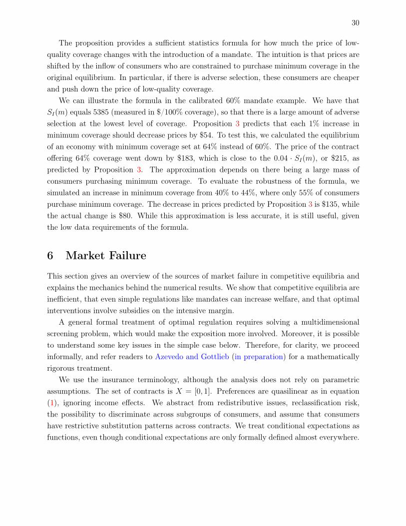
30

The proposition provides a sufficient statistics formula for how much the price of low-quality coverage changes with the introduction of a mandate. The intuition is that prices areshifted by the inflow of consumers who are constrained to purchase minimum coverage in theoriginal equilibrium. In particular, if there is adverse selection, these consumers are cheaperand push down the price of low-quality coverage.

We can illustrate the formula in the calibrated 60% mandate example. We have thatSI(m) equals 5385 (measured in $/100% coverage), so that there is a large amount of adverseselection at the lowest level of coverage. Proposition 3 predicts that each 1% increase inminimum coverage should decrease prices by $54. To test this, we calculated the equilibriumof an economy with minimum coverage set at 64% instead of 60%. The price of the contractoffering 64% coverage went down by $183, which is close to the 0.04 · SI(m), or $215, aspredicted by Proposition 3. The approximation depends on there being a large mass ofconsumers purchasing minimum coverage. To evaluate the robustness of the formula, wesimulated an increase in minimum coverage from 40% to 44%, where only 55% of consumerspurchase minimum coverage. The decrease in prices predicted by Proposition 3 is $135, whilethe actual change is $80. While this approximation is less accurate, it is still useful, giventhe low data requirements of the formula.

6 Market Failure

This section gives an overview of the sources of market failure in competitive equilibria andexplains the mechanics behind the numerical results. We show that competitive equilibria areinefficient, that even simple regulations like mandates can increase welfare, and that optimalinterventions involve subsidies on the intensive margin.

A general formal treatment of optimal regulation requires solving a multidimensionalscreening problem, which would make the exposition more involved. Moreover, it is possibleto understand some key issues in the simple case below. Therefore, for clarity, we proceedinformally, and refer readers to Azevedo and Gottlieb (in preparation) for a mathematicallyrigorous treatment.

We use the insurance terminology, although the analysis does not rely on parametricassumptions. The set of contracts is X = [0, 1]. Preferences are quasilinear as in equation(1), ignoring income effects. We abstract from redistributive issues, reclassification risk,the possibility to discriminate across subgroups of consumers, and assume that consumershave restrictive substitution patterns across contracts. We treat conditional expectations asfunctions, even though conditional expectations are only formally defined almost everywhere.

31

6.1 Inefficiency

We now show that the competitive equilibrium is inefficient when consumers have privateinformation about costs. In this sense, our model echoes the standard view of economists,regulators, and market participants that adverse and advantageous selection causes marketoutcomes to be inefficient.

Let ˆu− c dα (3)

denote the total surplus generated by the allocation α.31 We will consider total surplus as awelfare measure, and refer to it henceforth as welfare.32 Assume that cost, utility, and theendogenously determined price functions are continuously differentiable.

To understand the wedge between privately and socially optimal choices, fix a consumer θ.Denote marginal utility and marginal cost functions as mu(x, θ) = ∂xu(x, θ) and mc(x, θ) =

∂xc(x, θ). The consumer trades off the price against her willingness to pay for coverage, asin Figure 5. In an interior choice such as xeq, she equates marginal utility and the priceof an additional unit of coverage p′(x). However, the socially optimal choice xeff equatesmarginal utility and marginal cost. Therefore, whenever costs vary among consumers, thereis no reason to expect market outcomes to be efficient.

To understand the sources of inefficiency, define the intensive margin selection coefficientas

SI(x) = ∂xEx[c]− Ex[mc].

This measure is identical to the intensive margin selection coefficient at minimum coveragedefined in Section 5.3, but evaluated at contract x.

The wedge can be divided into two components. First, in a multidimensional model manydifferent types purchase contract x. This is the case in our calibrated example, as depictedin Figure 3b. Therefore, there is no reason for the marginal cost of any single buyer of x toequal p′(x). Second, even the average marginal cost Ex[mc] of consumers buying x may differfrom p′(x). The difference between p′(x) and Ex[mc] is SI(x), so these two quantities differwhenever there is advantageous or adverse selection. These two components are depicted in

31The literature sometimes refers to this measure as Kaldor-Hicks welfare, although this is only precise,according to the original definitions by Kaldor and by Hicks, in the case where a government has access tolump-sum transfers.

32Our basic analysis focuses on this particular welfare measure, as does much of the applied literature.However, constrained Pareto efficiency is also an important concept in the study of markets with adverseselection. Crocker and Snow (1985a) show that, in the Rothschild and Stiglitz model, the Miyazaki-Wilsonequilibrium is constrained Pareto efficient in that its allocations maximize the low-risk type’s utility subjectto incentive and zero profits constraints. The Riley equilibrium, which coincides with competitive equilibriumin the Rothschild and Stiglitz model, is only constrained efficient when it coincides with Miyazaki-Wilson.Therefore, in our model, equilibria may be constrained Pareto inefficient.

32

Ex[mc]

x

p′

muθ

mcθSI

xeq xeff

Figure 5: Inefficiency of private choices.

Notes: The figure illustrates the decision of an individual consumer θ. The privately optimal decision xeq isto equate marginal utility mu with the price of an additional unit of coverage p′. The socially optimal choicexeff equates marginal utility with marginal cost mc. The figure also depicts the average marginal cost curveof consumers purchasing contract xeq, in bold and denoted Ex[mc], and the marginal cost curves of otherconsumers purchasing xeq as faded curves.

Figure 5, where p′(x) is higher than the average marginal cost, implying that there is adverseselection.

6.2 Optimal Regulation and Risk Adjustment

Consider a government with no excess burden of public funds who wishes to regulate themarket to maximize welfare. The government can regulate the product space, prices, andemploy taxes and subsidies. However, it faces the same informational constraints as firms doand, therefore, cannot treat consumers differently conditional on their type.

Without loss of generality, the government’s problem is to choose an optimal price functionp(x), let consumers optimize reaching an allocation α, and make transfers t(x) per unit ofcontract x to firms so that they break even:

p(x) + t(x) = Ex[c].

That is, setting prices directly subsumes all other policy instruments. For example, forbiddinga contract is tantamount to setting a very high price.

We approach the problem of finding optimal prices from a sufficient statistics approachsimilar to Dixit and Sandmo (1977), Wilson (1993), Piketty (1997), Roberts (2000), and

33

Saez (2001). We consider a price schedule p(x), and perform a small perturbation p̃(x). Ifp(x) was originally optimal, then the perturbation p̃(x) should have a higher-order effect onwelfare. Our perturbation works as follows. Fix a contract x0. We increase the derivativep′(x) by dp′ in a small interval [x0, x0 + dx], and leave it unchanged otherwise. We make theadditional assumption that only adjustments in the intensive margin matter. That is, weassume that most of the welfare effects of this perturbation come from consumers who adjusttheir coverage in the intensive margin.

Under these assumptions, the welfare effect of the perturbation can be calculated asfollows. There are approximately f(x0) ·dx consumers who are affected by the change, wheref(x) is the density of consumers purchasing contract x. Each of these consumers reduces hercoverage by

ε(x0, θ) ·dp′

p′(x0)· x0,

where ε(x0, θ) is the intensive margin elasticity of coverage with respect to p′, defined in Sec-tion 5.3. Note that, although the perturbation extracts revenues from consumers purchasingcontracts higher than x0, this is moot because we are ignoring redistribution and there is noexcess cost of public funds. Therefore, the total welfare effect equals

Ex0 [ε · (mu−mc)] ·f(x0) · x0p′(x0)

· dxdp′

plus higher-order terms, which become insignificant as dx, dp′, and dp′/dx converge to 0.Consequently, optimal subsidies satisfy, for all x,

Ex[ε · (p′ −mc)] = 0.

This expectation can be decomposed as

0 = Ex[ε] · Ex[p′ −mc]− Covx[ε,mc]

= Ex[ε] · (SI(x)− t′(x))− Covx[ε,mc].

Rearranging this equation we find that optimal subsidies are given by33

t′(x)︸︷︷︸incremental subsidy

= SI(x)︸ ︷︷ ︸risk adjustment

− Covx[ε,mc]

Ex[ε]︸ ︷︷ ︸sorting

. (4)

The intuition for the optimal regulation formula is as follows. The term SI(x) compensates33We caution readers that this formula is not mathematically rigorous because conditional expectations

are only defined almost everywhere according to α.

34

firms for incremental costs that are due to selection. This term is closely related to riskadjustment, a common policy intervention in insurance markets. Actual risk-adjustmentpolicies cross-subsidize insurance plans based on observable enrollee characteristics that arepredictive of costs. Formulae differ in what characteristics are used, how expected costsare measured, and whether prospective or retrospective data is used. Both private andpublic sponsors use risk adjustment. For example, in employer-provided health insurance,plans are often priced according to expected costs of the average employee. Despite thesedifferences, and practical shortcomings of actual risk adjustment policies,34 policymakersand market participants often believe that it is important for cross subsidies to lean againstthe wind of advantageous or adverse selection, consistent with the SI(x) term. Moreover,the differences between the optimal subsidy and the usual risk-adjustment formulae clarifiesthat cross subsidies should fulfill economic objectives, as opposed to simply being equal toselection in a statistical sense. This is consistent with the shortcomings of purely statisticalrisk adjustment pointed out by Glazer and McGuire (2000) and Einav and Levin (2015).

To understand the intuition for the covariance term, recall the two sources of inefficiencyidentified in Section 6.1: marginal costs of any given consumer are different than the priceof additional coverage, and marginal costs and prices differ even on average. The risk-adjustment term SI(x) addresses this second source of inefficiency by eliminating adverse oradvantageous selection from the point of view of the firms. The covariance term deals withthe first source of inefficiency, which is due to the variation in marginal costs among differentbuyers of contract x. Hence, this term sorts consumers more efficiently. If buyers of x withhigher marginal costs also have more elastic demands, then the formula calls for a higherslope of prices p′(x) than under pure risk adjustment, which induces the high cost consumersto purchase lower levels of coverage. If this correlation is negative, then incremental pricesshould be lower, inducing consumers with lower costs to purchase more insurance.

This formula is consistent with the findings in Section 5. Namely, optimal prices in-volve cross subsidies on the intensive margin to reduce adverse selection not only in whetherconsumers participate in the market, but also in what kinds of contracts they buy.

Finally, our intuitive discussion considered the case where optimal regulation has aninterval of contracts being offered. However, we saw in the numerical simulations that,with higher heterogeneity in moral hazard, the optimal allocation may involve all consumerspurchasing the same contract. The intuition of why this can happen is simple. In theparametric example, the first-best contract for consumer θ can be calculated by equating

34Practical hurdles include measurement biases (Wennberg et al., 2013), gaming by firms (Brown et al.,2014; Geruso and Layton, 2015), and failure to capture all relevant dimensions of heterogeneity (Shepard,2014; Einav et al., 2015).

35

marginal utility and marginal cost, which gives

x =AθS

2θ

AθS2θ +Hθ

.

This expression is decreasing in the moral hazard parameter. All things equal, the socialplanner prefers to provide less coverage to consumers who are more likely to engage in moralhazard. However, consumers with higher moral hazard parameters always wish to purchasemore insurance. Hence, if all heterogeneity is in moral hazard, the planner prefers not toscreen consumers and, instead, assigns the same bundle to everyone. This phenomenon hasbeen described by Guesnerie and Laffont (1984) in one-dimensional screening models, whocall it non-responsiveness.

7 Conclusion

This paper considers a competitive model of adverse selection. Contract characteristics aredetermined endogenously and consumers may be heterogeneous across more than one dimen-sion, unlike standard models. Competitive equilibrium extends the Akerlof (1970) and Einavet al. (2010a) models beyond the case of a single contract, determining which contracts aretraded with supply and demand.

Equilibria are inefficient (in the sense of not maximizing total surplus) and even simpleinterventions such as mandates can increase welfare. Numerical examples suggest that stan-dard policies can have important unintended consequences. Policy interventions should takeinto account not only whether consumers participate in the market, but also policy effectson contract characteristics. This is in concert with the view of regulators, who often imple-ment policies aimed at affecting these characteristics, and with Einav et al. (2009), who havesuggested that contract characteristics may be important.

It would be interesting to test how well competitive equilibrium predicts behavior in mar-kets with adverse selection and to test it against alternative models. For example, in the caseof one dimension of heterogeneity there is considerable controversy over what a reasonableequilibrium notion is, despite many alternatives such as those proposed by Riley (1979) andMiyazaki (1977)-Wilson (1977). Unfortunately, these equilibria are defined in more restric-tive settings, so one cannot compare predictions in richer settings like our calibrated example.It would be interesting to extend these equilibrium notions to richer settings and comparetheir predictions to competitive equilibria.

36

References

Aizawa, Naoki and Hanming Fang, “Equilibrium Labor Market Search and Health In-surance Reform,” NBER Working Paper 18698, 2013.

Akerlof, George A, “The Market for “Lemons”: Quality Uncertainty and the Market Mech-anism,” Quarterly Journal of Economics, 1970, pp. 488–500.

Ambrus, Attila and Rossella Argenziano, “Asymmetric networks in two-sided markets,”American Economic Journal: Microeconomics, 2009, 1 (1), 17–52.

Attar, Andrea, Thomas Mariotti, and François Salanié, “Nonexclusive Competitionin the Market for Lemons,” Econometrica, 2011, 79 (6), 1869–1918.

Azevedo, Eduardo M and Daniel Gottlieb, “Non-Existence of Riley Equilibrium inMarkets with Adverse Selection,” Mimeo, University of Pennsylvania, 2016.

and , “Optimal Regulation of Markets with Adverse Selection,” Mimeo, University ofPennsylvania, in preparation.

Baicker, Katherine, Sendhil Mullainathan, and Joshua Schwartzstein, “BehavioralHazard in Health Insurance,” NBER Working Paper 18468, 2012.

Banks, Jeffrey S and Joel Sobel, “Equilibrium Selection in Signaling Games,” Economet-rica, 1987, pp. 647–661.

Billingsley, Patrick, Probability and Measure, John Wiley & Sons, 2008.

Bisin, Alberto and Piero Gottardi, “Competitive Equilibria with Asymmetric Informa-tion,” Journal of Economic Theory, 1999, 87 (1), 1–48.

and , “Efficient Competitive Equilibria with Adverse Selection,” Journal of PoliticalEconomy, 2006, 114 (3), 485–516.

Brown, Jason, Mark Duggan, Ilyana Kuziemko, and William Woolston, “How DoesRisk Selection Respond to Risk Adjustment? New Evidence from the Medicare AdvantageProgram,” American Economic Review, 2014, 104 (10), 3335–3364.

Chang, Briana, “Adverse Selection and Liquidity Distortion in Decentralized Markets,”Mimeo, Wisconsin School of Business, 2010.

Chen, Ying, Navin Kartik, and Joel Sobel, “Selecting Cheap-Talk Equilibria,” Econo-metrica, 2008, 76 (1), 117–136.

37

Chiappori, Pierre-André and Bernard Salanié, “Testing for Asymmetric Informationin Insurance Markets,” Journal of Political Economy, 2000, 108 (1), 56–78.

, Bruno Jullien, Bernard Salanié, and Francois Salanié, “Asymmetric Informationin Insurance: General Testable Implications,” Rand Journal of Economics, 2006, 37 (4),783–798.

, Robert J McCann, and Lars P Nesheim, “Hedonic Price Equilibria, Stable Match-ing, and Optimal Transport: Equivalence, Topology, and Uniqueness,” Economic Theory,2010, 42 (2), 317–354.

Cho, In-Koo and David M Kreps, “Signaling Games and Stable Equilibria,” QuarterlyJournal of Economics, 1987, pp. 179–221.

Citanna, Alessandro and Paolo Siconolfi, “Refinements and Incentive Efficiency in Wal-rasian Models of Insurance Economies,” Journal of Mathematical Economics, 2014, 50,208–218.

Cohen, Alma and Liran Einav, “Estimating Risk Preferences from Deductible Choice,”American Economic Review, 2007, 97 (3), 745–788.

Crocker, Keith J. and Arthur Snow, “The Efficiency of Competitive Equilibria in Insur-ance Markets with Asymmetric Information,” Journal of Public Economics, 1985a, 26 (2),207–219.

Cutler, David M and Sarah Reber, “Paying for Health Insurance: The Trade-off betweenCompetition and Adverse Selection,” Quarterly Journal of Economics, 1998, 113 (2).

Dafny, Leemore, Mark Duggan, and Subramaniam Ramanarayanan, “Paying a Pre-mium on Your Premium? Consolidation in the Us Health Insurance Industry,” AmericanEconomic Review, 2012, 102 (2), 1161–1185.

Dafny, Leemore S, “Are Health Insurance Markets Competitive?,” American EconomicReview, 2010, 100 (4), 1399–1431.

Decarolis, Francesco, Maria Polyakova, and Stephen Ryan, “The Welfare Effects ofSupply Side Regulations in Medicare Part D,” Mimeo, Stanford University, 2012.

Dixit, Avinash and Agnar Sandmo, “Some Simplified Formulae for Optimal IncomeTaxation,” The Scandinavian Journal of Economics, 1977, pp. 417–423.

Dubey, Pradeep and John Geanakoplos, “Competitive Pooling: Rothschild-Stiglitz Re-considered,” Quarterly Journal of Economics, 2002, pp. 1529–1570.

38

, , and Martin Shubik, “Default and Punishment in General Equilibrium,” Economet-rica, 2005, pp. 1–37.

Einav, L, A Finkelstein, and J Levin, “Beyond Testing: Empirical Models of InsuranceMarkets.,” Annual Review of Economics, 2009, 2, 311–336.

Einav, Liran, Amy Finkelstein, and Mark R Cullen, “Estimating Welfare in InsuranceMarkets Using Variation in Prices,” Quarterly Journal of Economics, 2010, 125 (3), 877–921.

, , and Paul Schrimpf, “Optimal Mandates and the Welfare Cost of AsymmetricInformation: Evidence from the UK Annuity Market,” Econometrica, 2010, 78 (3), 1031–1092.

, , Raymond Kluender, and Paul Schrimpf, “Beyond Statistics: The EconomicContent of Risk Scores,” Mimeo, Stanford University, 2015.

, , Stephen P Ryan, Paul Schrimpf, and Mark R Cullen, “Selection on MoralHazard in Health Insurance,” American Economic Review, 2013, 103 (1), 178–219.

and , “Selection in Insurance Markets: Theory and Empirics in Pictures,” Journal ofEconomic Perspectives, 2011, 25 (1), 115–138.

and Jonathan D Levin, “Managed Competition in Health Insurance,” Mimeo, StanfordUniversity, 2015.

Fang, Hanming, Michael P Keane, and Dan Silverman, “Sources of AdvantageousSelection: Evidence from the Medigap Insurance Market,” Journal of Political Economy,2008, 116 (2), 303–350.

Finkelstein, Amy and Kathleen McGarry, “Multiple Dimensions of Private Information:Evidence from the Long-Term Care Insurance Market,” American Economic Review, 2006,96 (4), 938–958.

Gale, Douglas, “A Walrasian Theory of Markets with Adverse Selection,” The Review ofEconomic Studies, 1992, 59 (2), 229–255.

Geruso, Michael and Timothy Layton, “Upcoding or Selection? Evidence from Medicareon Squishy Risk Adjustment,” NBER Working Paper 21222, 2015.

Glazer, Jacob and Thomas G McGuire, “Optimal Risk Adjustment in Markets withAdverse Selection: An Application to Managed Care,” American Economic Review, 2000,pp. 1055–1071.

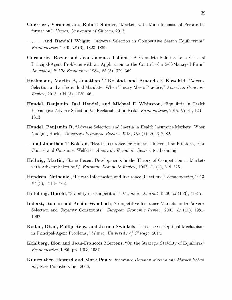
39

Guerrieri, Veronica and Robert Shimer, “Markets with Multidimensional Private In-formation,” Mimeo, University of Chicago, 2013.

, , and Randall Wright, “Adverse Selection in Competitive Search Equilibrium,”Econometrica, 2010, 78 (6), 1823–1862.

Guesnerie, Roger and Jean-Jacques Laffont, “A Complete Solution to a Class ofPrincipal-Agent Problems with an Application to the Control of a Self-Managed Firm,”Journal of Public Economics, 1984, 25 (3), 329–369.

Hackmann, Martin B, Jonathan T Kolstad, and Amanda E Kowalski, “AdverseSelection and an Individual Mandate: When Theory Meets Practice,” American EconomicReview, 2015, 105 (3), 1030–66.

Handel, Benjamin, Igal Hendel, and Michael D Whinston, “Equilibria in HealthExchanges: Adverse Selection Vs. Reclassification Risk,” Econometrica, 2015, 83 (4), 1261–1313.

Handel, Benjamin R, “Adverse Selection and Inertia in Health Insurance Markets: WhenNudging Hurts,” American Economic Review, 2013, 103 (7), 2643–2682.

and Jonathan T Kolstad, “Health Insurance for Humans: Information Frictions, PlanChoice, and Consumer Welfare,” American Economic Review, forthcoming.

Hellwig, Martin, “Some Recent Developments in the Theory of Competition in Marketswith Adverse Selection*,” European Economic Review, 1987, 31 (1), 319–325.

Hendren, Nathaniel, “Private Information and Insurance Rejections,” Econometrica, 2013,81 (5), 1713–1762.

Hotelling, Harold, “Stability in Competition,” Economic Journal, 1929, 39 (153), 41–57.

Inderst, Roman and Achim Wambach, “Competitive Insurance Markets under AdverseSelection and Capacity Constraints,” European Economic Review, 2001, 45 (10), 1981–1992.

Kadan, Ohad, Philip Reny, and Jeroen Swinkels, “Existence of Optimal Mechanismsin Principal-Agent Problems,” Mimeo, University of Chicago, 2014.

Kohlberg, Elon and Jean-Francois Mertens, “On the Strategic Stability of Equilibria,”Econometrica, 1986, pp. 1003–1037.

Kunreuther, Howard and Mark Pauly, Insurance Decision-Making and Market Behav-ior, Now Publishers Inc, 2006.

40

Luz, Vitor F., “Characterization and Uniqueness of Equilibrium in Competitive Insurance,”Mimeo, Yale University, 2013.

Mahoney, Neale and E Glen Weyl, “Imperfect Competition in Selection Markets,”Mimeo, University of Chicago, 2014.

Mailath, George J, Masahiro Okuno-Fujiwara, and Andrew Postlewaite, “Belief-Based Refinements in Signalling Games,” Journal of Economic Theory, 1993, 60 (2), 241–276.

Miyazaki, Hajime, “The Rat Race and Internal Labor Markets,” Bell Journal of Economics,1977, pp. 394–418.

Myerson, Roger B, “Refinements of the Nash Equilibrium Concept,” International Journalof Game Theory, 1978, 7 (2), 73–80.

, “Sustainable Matching Plans with Adverse Selection,” Games and Economic Behavior,1995, 9 (1), 35–65.

Netzer, Nick and Florian Scheuer, “Competitive Screening in Insurance Markets withEndogenous Wealth Heterogeneity,” Economic Theory, 2010, 44 (2), 187–211.

and , “A Game Theoretic Foundation of Competitive Equilibria with Adverse Selection,”International Economic Review, 2014, 55 (2), 399–422.

Novshek, William and Hugo Sonnenschein, “General equilibrium with free entry: asynthetic approach to the theory of perfect competition,” Journal of Economic Literature,1987, 25 (3), 1281–1306.

Pauly, Mark V, Olivia S Mitchell, and Yuhui Zeng, “Death Spiral or Euthanasia? TheDemise of Generous Group Health Insurance Coverage,” Inquiry, 2007, pp. 412–427.

Piketty, Thomas, “La Redistribution Fiscale Face Au Chômage,” Revue FrançaiseD’Économie, 1997, 12 (1), 157–201.

Plott, Charles R and Glen George, “Marshallian vs. Walrasian stability in an experi-mental market,” The Economic Journal, 1992, 102 (412), 437–460.

Polyakova, Maria, “Regulation of Insurance with Adverse Selection and Switching Costs:Evidence from Medicare Part D,” Mimeo, Stanford University, 2014.

Prescott, Edward C and Robert M Townsend, “Pareto Optima and Competitive Equi-libria with Adverse Selection and Moral Hazard,” Econometrica, 1984, pp. 21–45.

41

Rabin, Matthew, “Risk Aversion and Expected-Utility Theory: A Calibration Theorem,”Econometrica, 2000, 68 (5), 1281–1292.

Riley, John G, “Informational Equilibrium,” Econometrica, 1979, pp. 331–359.

Roberts, Kevin, “A Reconsideration of the Optimal Income Tax,” in Peter Hammond andGareth Myles, eds., Incentives, Organization, and Public Economics: Papers in Honour ofSir James Mirrlees, Oxford University Press, 2000.

Rochet, Jean-Charles and Lars A Stole, “Nonlinear Pricing with Random Participa-tion,” Review of Economic Studies, 2002, 69 (1), 277–311.

Rothschild, Michael and Joseph Stiglitz, “Equilibrium in Competitive Insurance Mar-kets: An Essay on the Economics of Imperfect Information,” Quarterly Journal of Eco-nomics, 1976, 90 (4), 629–649.

Saez, Emmanuel, “Using Elasticities to Derive Optimal Income Tax Rates,” Review ofEconomic Studies, 2001, 68 (1), 205–229.

Scheuer, Florian and Kent A Smetters, “Could a Website Really Have Doomed theHealth Exchanges? Multiple Equilibria, Initial Conditions and the Construction of theFine,” NBER Working Paper 19835, 2014.

Shepard, Mark, “Hospital Network Competition and Adverse Selection: Evidence from theMassachusetts Health Insurance Exchange,” Mimeo, Harvard University, 2014.

Spence, A Michael, “Monopoly, Quality, and Regulation,” Bell Journal of Economics,1975, pp. 417–429.

Spence, Michael, “Job Market Signaling,” Quarterly Journal of Economics, 1973, pp. 355–374.

Spinnewijn, Johannes, “Unemployed but Optimistic: Optimal Insurance Design with Bi-ased Beliefs,” Journal of the European Economic Association, February 2015, 13 (1), 130–167.

Starc, Amanda, “Insurer Pricing and Consumer Welfare: Evidence from Medigap,” TheRand Journal of Economics, 2014, 45 (1), 198–220.

Tebaldi, Pietro, “Estimating Equilibrium in Health Insurance Exchanges: Price Competi-tion and Subsidy Design under the ACA,” Mimeo, Stanford University, 2015.

42

Van de Ven, Wynand PMM and Randall P Ellis, “Risk Adjustment in CompetitiveHealth Plan Markets,” in A J Culyer and Joseph P Newhouse, eds., Handbook of HealthEconomics, 1999.

Veiga, André and E Glen Weyl, “The Leibniz Rule for Multidimensional Heterogeneity,”Mimeo, University of Chicago, 2014.

and , “Product Design in Selection Markets,” Mimeo, University of Chicago, 2014.

Wennberg, John E, Douglas O Staiger, Sandra M Sharp, Daniel J Gottlieb,Gwyn Bevan, Klim McPherson, and H Gilbert Welch, “Observational IntensityBias Associated with Illness Adjustment: Cross Sectional Analysis of Insurance Claims,”British Medical Journal, 2013, 346.

Wilson, Charles, “A Model of Insurance Markets with Incomplete Information,” Journalof Economic Theory, 1977, 16 (2), 167–207.

, “The Nature of Equilibrium in Markets with Adverse Selection,” Bell Journal of Eco-nomics, 1980, pp. 108–130.

Wilson, Robert B, Nonlinear Pricing, Oxford University Press, 1993.