Performance-Aligned Learning Algorithms with Statistical Guarantees

1

Rizal Zaini Ahmad FathonyCommittee: Prof. Brian Ziebart (Chair)

Prof. Bhaskar DasGuptaProf. Xinhua ZhangProf. Lev ReyzinProf. Simon Lacoste-Julien

2

Outline

Introduction & Motivation1

General Multiclass Classification2

Graphical Models3

Bipartite Matching in Graphs4

Conclusion & Future Directions5

“New learning algorithms that align with performance/loss metrics and provide the statistical guarantees of Fisher consistency”

Introduction and Motivation

3

Data

DataDistribution𝑃(𝒙, 𝑦)

𝒙1 𝑦1

𝒙2 𝑦2

𝒙𝑛 𝑦𝑛

…

Training

Supervised Learning

𝒙𝑛+1 ො𝑦𝑛+1

Testing

𝒙𝑛+2

…

Loss/Performance Metrics:loss ො𝑦, 𝑦 / score( ො𝑦, 𝑦)

4

ො𝑦𝑛+2

Multiclass Classification

• Zero one loss / accuracy metric• Absolute loss (for ordinal regression)

Multivariate Performance

• F1-score• Precision@k

Structured Prediction

• Hamming loss (sum of 0-1 loss)

5

• Assume a family of parametric hypothesis function 𝑓 (e.g. linear discriminator)

• Find the hypothesis 𝑓∗ that minimize the empirical risk:

Non-convex, non-continuous metrics → Intractable optimization

Convex surrogate loss need to be employed!

Empirical Risk Minimization (ERM) (Vapnik, 1992)

Fisher ConsistencyUnder ideal condition: optimize surrogate→minimizes the loss metric(given the true distribution and fully expressive model)

A desirable property of convex surrogates:

6

Two Main Approaches

Probabilistic Approach1

Large-Margin Approach2

• Construct prediction probability model

• Employ the logistic loss surrogate

Logistic Regression, Conditional Random Fields (CRF)

• Maximize the margin that separates correct prediction from the incorrect one

• Employ the hinge loss surrogate

Support Vector Machine (SVM), Structured SVM

* Pictures are taken from MLPP book (Kevin Murphy)

7

Multiclass Classification | Logistic Regression vs SVM

Multiclass Logistic Regression1 Multiclass SVM2

Statistical guarantee of Fisher consistency(minimizes the zero-one loss metric in the limit)

No dual parameter sparsityComputational efficiency (via the kernel trick & dual parameter sparsity)

Current multiclass SVM formulations:

- Lack Fisher consistency property, or- Doesn’t perform well in practice

8

Structured Prediction| CRF vs Structured SVM

Conditional Random Fields (CRF)1 Structured SVM2

No easy mechanism to incorporatecustomized loss/performance metrics

Flexibility to incorporate customized loss/performance metrics

Computation of the normalization termmay be intractable

Relatively more efficient in computation

Statistical guarantee of Fisher consistency No Fisher consistency guaranteees

9

New Learning Algorithms?

Provide Fisher consistency guarantee

Align better with the loss/performance metric(by incorporating the metric into its learning objective)

Computationally efficient

Perform well in practiceHow?

“What predictor best maximizes the performance metric (or minimizes the loss metric) in the worst case given the statistical summaries of the empirical distributions?”

Robust adversarial learning approach

Performance-Aligned Surrogate Losses for General Multiclass Classification

10

Based on:

Fathony, R., Asif, K., Liu, A., Bashiri, M. A., Xing, W., Behpour, S., Zhang, X., and Ziebart, B. D.: Consistent robust adversarial prediction for general multiclass classification. arXiv preprint arXiv:1812.07526, 2018. (Submitted to JMLR).

Fathony, R., Liu, A., Asif, K., and Ziebart, B.: Adversarial multiclass classification: A risk minimization perspective. NIPS 2016.

Fathony, R., Bashiri, M. A., and Ziebart, B.: Adversarial surrogate losses for ordinal regression. NIPS 2017.

Data

DataDistribution𝑃(𝒙, 𝑦)

𝒙1 𝑦1

𝒙2 𝑦2

𝒙𝑛 𝑦𝑛

…

Training

Supervised Learning | Multiclass Classification

𝒙𝑛+1 ො𝑦𝑛+1

Testing

𝒙𝑛+2

…

Loss/Performance Metrics:loss ො𝑦, 𝑦 / score( ො𝑦, 𝑦)

11

ො𝑦𝑛+2

…

1

2

3

𝑘

Finite set of possible

value of 𝑦

12

Multiclass Classification | Zero-One Loss

Example: Digit Recognition

…

1

2

3

…

Loss Metric:loss ො𝑦, 𝑦 = 𝐼(ො𝑦 ≠ 𝑦)

Loss Metric: Zero-One Loss

L =

13

Multiclass Classification | Ordinal Classification

Loss Metric:loss ො𝑦, 𝑦 = | ො𝑦 − 𝑦|

Loss Metric: Absolute Loss

L =

…

1

2

5

…

Predicted vs Actual Label:

Distance Loss

Example: Movie Rating Prediction

14

Multiclass Classification | Classification with Abstention

Predictor can say ‘abstain’

1

2

3

Loss Metric:

loss ො𝑦, 𝑦 = ቊ𝛼 if abstain

𝐼( ො𝑦 ≠ 𝑦) otherwise

Loss Metric: Abstention Loss

L =

Prediction

Abstain

15

Multiclass Classification | Other Loss Metrics

Squared loss metric

loss ො𝑦, 𝑦 = ො𝑦 − 𝑦 2

Cost-sensitive loss metricTaxonomy-based loss metric

loss ො𝑦, 𝑦 = ℎ − 𝑣 ො𝑦, 𝑦 + 1 loss ො𝑦, 𝑦 = 𝐂 ො𝑦,𝑦

Robust Adversarial Learning

16

17

Robust Adversarial Learning (Grunwald & Dawid, 2004; Delage & Ye, 2010; Asif et.al, 2015)

Empirical Risk MinimizationApproximate the lossOriginal Loss MetricNon-convex, non-continuous with convex surrogates

Probabilistic prediction

Evaluate against an adversary,instead of using empirical data

Adversary’s probabilistic predictionConstraint the statistics ofthe adversary’s distributionto match the empirical statistics

Robust Adversarial Learning

18

Robust Adversarial Dual Formulation

Primal:

Dual:

Lagrange multiplier, minimax duality

ERM with the adversarial surrogate loss (AL):

Simplified notation

where:

Convex in 𝜃

19

Adversarial Surrogate Loss

Adversarial Surrogate Loss

Convert to a Linear Program

Convex Polytope formed by the constraints

Example for a four class classification

Extreme points of the (bounded) polytope

There is always an optimal solution that is an extreme point of the domain.

Computing AL = finding the best extreme point

LP Solver𝑂(𝑘3.5)

20

Zero-One Loss : AL0-1| Convex Polytope

Extreme points of the polytope

The Adversarial Surrogate Loss for Zero-One Loss Metrics (AL0-1)

Computation of AL0-1

- Sort 𝑓𝑖 in non-increasing order- Incrementally add potentials to the set 𝑆,

until adding more potential decrease the loss value

O(𝑘 log 𝑘), where 𝑘 is the number of classes𝒆𝑖 is a vector with a single 1 at the i-th index,and 0 elsewhere.

Convex Polytope of the AL0-1

21

AL0-1| Loss Surface

Binary Classification

Three Class Classification

- Plots over the space of potential differences 𝜓𝑖 = 𝑓𝑖 − 𝑓𝑦- The true label is 𝑦 = 1

22

Other Multiclass Loss Metrics

Extreme points of the polytope:

𝒆𝑖 is a vector with a single 1 at the i-th index,and 0 elsewhere.

Ordinal Regression with Absolute Loss Metric

Adversarial Surrogate Loss ALord:

Computation cost:O(𝑘), where 𝑘 is the number of classes

23

Other Multiclass Loss Metrics

Extreme points of the polytope:

𝒆𝑖 is a vector with a single 1 at the i-th index,and 0 elsewhere.

Classification with Abstention (0 ≤ 𝛼 ≤ 0.5)

Adversarial Surrogate Loss ALabstain:

Computation cost:O(𝑘), where 𝑘 is the number of classes

24

Fisher Consistency

Fisher Consistency Requirement in Multiclass Classification

- 𝑃(𝑌|𝒙) is the true conditional distribution- 𝑓 is optimized over all measurable functions

Consistency

Fisher consistent

Bayes risk minimizer

Minimizer Property- 𝐝 is the true conditional distribution- 𝑦⋄is the Bayes optimal predictor

Under 𝐟∗:

25

Optimization

Sub-gradient descent

Incorporate Rich Feature Spaces via the Kernel Trick

input space𝒙𝑖

rich feature space𝜔(𝒙𝑖)

Compute the dot products

1. Dual Optimization (benefit: dual parameter sparsity)

2. Primal Optimization (via PEGASOS (Shalev-Shwartz, 2010))

𝑆∗ is the set that maximize AL0-1

Example: AL0-1

Experiments:Example: Multiclass Classification (0-1 loss)

26

27

Multiclass Classification | Related Works

1. The WW Model (Weston et.al., 2002)

Multiclass Support Vector Machine (SVM)

2. The CS Model (Crammer and Singer, 1999)

3. The LLW Model (Lee et.al., 2004)

with:

Fisher Consistent?(Tewari and Bartlett, 2007)

(Liu, 2007)

Perform well inlow dimensional feature?

(Dogan et.al., 2016)

Relative Margin Model

Relative Margin Model

Absolute Margin Model

28

AL0-1 | Experiments

Dataset properties and AL0-1 constraints

12 datasets dual parameter sparsity

29

AL0-1 | Experiments | Results

Results for Linear Kernel and Gaussian Kernel

The mean (standard deviation) of the accuracy. Bold numbers: best or not significantly worse than the best

Linear KernelAL01: slight benefitLLW: poor perf.

Gauss. KernelLLW: improved perf.AL01: maintain benefit

30

Multiclass Zero-One Classification

1. The SVM WW Model (Weston et.al., 2002)

2. The SVM CS Model (Crammer and Singer, 1999)

3. The SVM LLW Model (Lee et.al., 2004)

Fisher Consistent?Perform well in

low dimensional feature?

Relative Margin Model

Relative Margin Model

Absolute Margin Model

4. The AL0-1 (Adversarial Surrogate Loss)Relative Margin Model

Other resultsGeneral Multiclass Classification

31

General Multiclass Classification

1. Zero-One Loss Metric

2. Ordinal Classification with the Absolute Loss Metric

3. Ordinal Classification with the Squared Loss Metric

4. Weighted Multiclass Loss Metrics

5. Classification with Abstention / Reject Option

Performance-Aligned Graphical Models

32

Based on:

Rizal Fathony, Ashkan Rezaei, Mohammad Bashiri, Xinhua Zhang, Brian D. Ziebart. “Distributionally Robust Graphical Models”. Advances in Neural Information Processing Systems 31 (NIPS), 2018

33

Conditional Graphical Models

Some Popular Graphical Structure in Structured Prediction

Chain Structure

Tree Structure

Lattice Structure

Activity Prediction, Sequence Tagging, NLP tasks: e.g. Named Entity Recognition

Parse Tree-Based NLP tasks:Semantic Role Labeling and Sentiment Analysis

Computer Vision Tasks:e.g. Image Segmentation

34

Previous Approaches for Conditional Graphical Models

Conditional Random Fields (CRF)1

Structured SVM (SSVM)2

Fisher ConsistentProduce Bayes optimal prediction in ideal case.

No easy mechanism to incorporatecustomized loss/performance metricsThe algorithm optimized the conditional likelihood.Loss/performance metric-based predictioncan be performed after learning process.

Align with the loss/performance metricsThe algorithm accept customized loss/performance metric in its optimization objective.

No Fisher consistency guaranteeBased on Multiclass SVM-CS.Not consistent for distribution with no majority label.

(Tsochantaridis et. al., 2005)(Lafferty et. al., 2001)

35

Adversarial Graphical Models (AGM)

Primal:

- Feature function Φ 𝐗, 𝐘 is additively decomposed over cliques, Φ 𝐱, 𝐲 = σcϕ x, yc

- The loss metric is additively decomposed over each 𝑦𝑖 variables, loss ෝ𝒚, 𝒚 = σi=1n loss ෝyi, yi

- Focus on pairwise graphical models: interactions between label = edges in graphs

Dual:

𝜃𝑒: Lagrange multipliers for constraints with edge features𝜃𝑣: Lagrange multipliers for constraints with node features

size:𝑘𝑛 × 𝑘𝑛

Intractablefor modestly-sized 𝑛

36

AGM | Marginal Formulation

Dual | Marginal Formulation:

The objective depends on 𝑃(ො𝐲|𝐱) only through its node marginal probability 𝑃(ෝ𝑦𝑖|𝐱)

The objective depends on ෘ𝑃(�ු�|𝐱) only through its node and edge marginal probability ෘ𝑃(𝑦𝑖|𝐱) and ෘ𝑃(𝑦𝑖 , 𝑦𝑗|𝐱)

General Graphical Models:Intractable

Similar to CRF and SSVM:

Focus:Graphs with low tree-width,e.g.: chain, tree, simple loops.

Tractable optimization

Dual:

37

AGM | Optimization

Matrix Notation (Tree Structure AGM):

- Stochastic (sub)-gradient descent

(outer optimization for 𝜃𝑒 and 𝜃𝑣)

- Dual decomposition (inner 𝐐 optimization)

- Discrete optimal transport solver (recovering 𝐐)

- Closed-form solution (inner 𝐩 optimization)

Optimization Techniques: - Depends on the loss metric used - For the additive zero-one loss (Hamming loss)

𝑂(𝑛𝑙𝑘 log 𝑘 + 𝑛𝑘2)𝑘: # classes, 𝑛: # nodes, 𝑙: # iterations in dual decomposition

Runtime (for a single subgradient update):

CRF𝑂(𝑛𝑘2)

SSVM𝑂(𝑛𝑘2)

General graphs low tree-width

𝑂 𝑛𝑙𝑤𝑘(𝑤+1) log 𝑘 + 𝑛𝑘2(𝑤+1)

𝑛: # cliques, 𝑤: treewidth of the graph

38

AGM | Consistency

when 𝑓 is optimized over all measurable functions on the input space

AGM is consistent

when 𝑓 is optimized over a restricted set of functions:

all measurable function that are additive over the edge and node potentials.

AGM is also consistent

If the loss function is additive

39

AGM | Experiments (1)

Facial Emotion Intensity Prediction (Chain Structure, Labels with Ordinal Category)

- Each node: 3 class classification: neutral = 1< increasing = 2 < apex = 3- 167 sequences- Ordinal loss metrics: zero-one loss, absolute loss, and squared loss- Weighted and unweighted. Weights reflect the focus of prediction (e.g. focus more on latest nodes)

Results: The mean (standard deviation) of the average loss metrics. Bold numbers: best or not significantly worse than the best

40

AGM | Experiments (2)

Semantic Role Labeling (Tree Structure)

- Predict label of each node given known parse tree.- CoNLL 2005 dataset- Cost-sensitive loss metric is used reflect the importance of each label

Results:

41

Conditional Graphical Models

Performance-Aligned?

Conditional Random Field (CRF)

Structured SVM

Adversarial Graphical Models

(Lafferty et. al., 2001)

(Tsochantaridis et. al., 2005)

(our approach)

Consistent?

Bipartite Matching in Graphs

42

Based on:

Rizal Fathony*, Sima Behpour*, Xinhua Zhang, Brian D. Ziebart. “Efficient and Consistent Adversarial Bipartite Matching”. International Conference on Machine Learning (ICML), 2018.

43

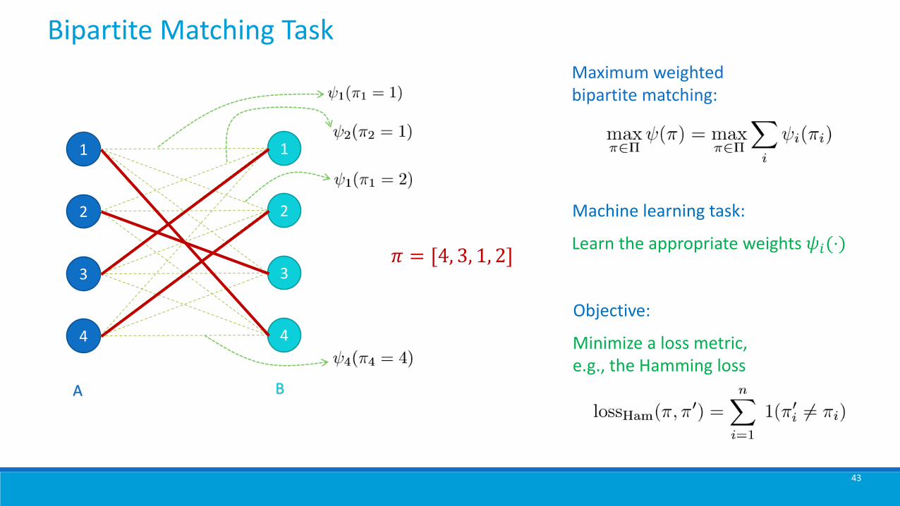
Bipartite Matching Task

Maximum weighted bipartite matching:

1

2

3

4

1

2

3

4

A B

𝜋 = [4, 3, 1, 2]

Machine learning task:

Learn the appropriate weights 𝜓𝑖(⋅)

Objective:

Minimize a loss metric,e.g., the Hamming loss

44

Learning Bipartite Matching | Applications

Word alignment (Taskar et. al., 2005; Pado & Lapta, 2006; Mac-Cartney et. al., 2008)

1

natürlich ist das haus klein

of course the house is small

Correspondence between images (Belongie et. al., 2002; Dellaert et. al., 2003)

2

Learning to rank documents (Dwork et. al., 2001; Le & Smola, 2007)

3

1

2

3

4

A non-bipartite matching task can be converted to a bipartite matching problem

45

Previous Approaches for Bipartite Matching

CRF1 Structured SVM2

Fisher ConsistentProduce Bayes optimal prediction in ideal case

Computationally intractableNormalization term requires matrix permanentcomputation (a #P-hard problem). Approximation is needed for modestly sized problems.

Computationally EfficientHungarian algorithm for computing the maximum violated constraints

No Fisher consistency guaranteeBased on Multiclass SVM-CSNot consistent for distribution with no majority label

solved using constraint generation

(Tsochantaridis et. al., 2005)(Petterson et. al., 2009; Volkovs & Zemel, 2012)

46

Adversarial Bipartite Matching (our approach)

Primal:

Dual:

Hamming loss Lagrangian term 𝛿

Augmented Hamming loss matrix for 𝑛 = 3 permutations

size:𝑛! × 𝑛!

Intractablefor modestly-sized 𝑛

47

Polytope of the Permutation Mixtures

Marginal Distribution Matrices:

Predictor

Adversary

𝐏 =

𝐐 =

𝑝𝑖,𝑗 = 𝑃(ො𝜋𝑖 = 𝑗)

𝑞𝑖,𝑗 = ෘ𝑃 ( 𝜋𝑖 = 𝑗)

Dual:

Birkhoff – Von Neumann theorem:

123

132

213231

312

321convex polytope whose points aredoubly stochastic matrices

reduce the space of optimization:

from 𝑂(𝑛!) to 𝑂(𝑛2)

48

Marginal Distribution Formulation

Dual:

Marginal Formulation:

- Outer (Q) : projected Quasi-Newton (Schmidt, et.al., 2009)

- Inner (𝜃) : closed-form solution

- Inner (P) : projection to doubly-stochastic matrix

- Projection to doubly-stochastic matrix : ADMM

Optimization Techniques Used:

Rearrange the optimization order and add regularization and smoothing penalties

49

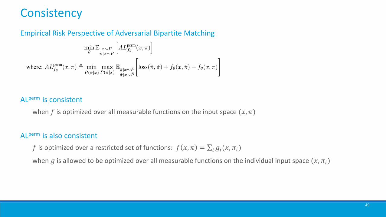
Consistency

Empirical Risk Perspective of Adversarial Bipartite Matching

when 𝑓 is optimized over all measurable functions on the input space (𝑥, 𝜋)

ALperm is consistent

𝑓 is optimized over a restricted set of functions: 𝑓 𝑥, 𝜋 = σ𝑖 𝑔𝑖(𝑥, 𝜋𝑖)

when 𝑔 is allowed to be optimized over all measurable functions on the individual input space (𝑥, 𝜋𝑖)

ALperm is also consistent

50

Experiments

1.01.31.52.52.8

1.01.21.44.25.0

relative: 12=1.0 relative: 1.96=1.0

Application: Video Tracking

Empirical runtime (until convergence)

Adversarial. Marginal Formulation:grows (roughly) quadratically in 𝑛

CRF: impractical even for 𝑛 = 20(Petterson et. al., 2009)

Public Benchmark Datasets

51

Experiment Results

6 pairs of dataset

significantly outperforms SSVM

2 pairs of dataset

competitive with SSVM

52

Bipartite Matching in Graphs

Efficient? Perform well?

Conditional Random Field (CRF)

Structured SVM

Adversarial Bipartite Matching

(Petterson et. al., 2009; Volkovs & Zemel, 2012)

(Tsochantaridis et. al., 2005)

(our approach)

Consistent?

?

Conclusion

53

54

Robust Adversarial Learning Algorithms

Provide Fisher consistency guarantee

Align better with the loss/performance metric(by incorporating the metric into its learning objective)

Computationally efficient

Perform well in practice

Future Directions

55

56

Future Directions (1)

1. Fairness in Machine Learning

Our formulation only enforces constraints on the adversary.

Add fairness constraints to the predictor?

Important issues in automated decision using ML algorithms.

Requires the algorithm to producefair prediction.

2. Statistical Theory of Loss Functions

Is there any stronger statistical guarantee that can separate the high-performing Fisher consistent algorithm from the low-performing ones?

In multiclass classification problem, both AL0-1 and SVM-LLW are Fisher consistent.However, their performances are quite different.

57

Future Directions (2)

3. Structured Prediction & Graphical Models

4. Deep Learning

Can we develop learning algorithms for general graphical models?

More complex graphical structures are popular in some applications, e.g. computer vision.

Deep learning has been successfully applied to many prediction problems.

How can the robust adversarial learning approach help designing deep learning architectures?What kind of approximation algorithms can be

applicable?

Exact learning algorithms for AGM in this case may be intractable.

Most of deep learning architecturesare not designed to optimize customized loss metrics.

58

Collaborators

MB

Mohammad Bashiri

AR

Ashkan Rezaei

KA

Kaiser Asif

AL

Anqi Liu

SB

Sima Behpour

XZ

Prof. Xinhua Zhang

BZ

Prof. Brian Ziebart

WX

Wei Xing

59

Publications

• Consistent Robust Adversarial Prediction for General Multiclass ClassificationRizal Fathony, Kaiser Asif, Anqi Liu, Mohammad Bashiri, Wei Xing, Sima Behpour, Xinhua Zhang, Brian D. Ziebart. Submitted to JMLR.

• Distributionally Robust Graphical Models Rizal Fathony, Ashkan Rezaei, Mohammad Bashiri, Xinhua Zhang, Brian D. Ziebart. Advances in Neural Information Processing Systems 31 (NeurIPS), 2018.

• Efficient and Consistent Adversarial Bipartite MatchingRizal Fathony*, Sima Behpour*, Xinhua Zhang, Brian D. Ziebart. International Conference on Machine Learning (ICML), 2018.

• Adversarial Surrogate Losses for Ordinal Regression Rizal Fathony, Mohammad Bashiri, Brian D. Ziebart. Advances in Neural Information Processing Systems 30 (NIPS), 2017.

• Adversarial Multiclass Classification: A Risk Minimization PerspectiveRizal Fathony, Anqi Liu, Kaiser Asif, Brian D. Ziebart. Advances in Neural Information Processing Systems 29 (NIPS), 2016.

• Kernel Robust Bias-Aware Prediction under Covariate Shift Anqi Liu, Rizal Fathony, Brian D. Ziebart. ArXiv Preprints, 2016.

Thank You

60