performance analysis of production systems methods for

1

Performance analysis of

production systems –

methods for reliability

and availability analysis

Marco Macchi

2

Performance framework

Assistenza Tecnica

Capitale

Risorse

produttive

Interne Esterne

Produttività

Di conformità

Affidabilità

Qualità

Di progetto

Tempestività

Puntualità

Servizio

Personalizzazione

Di mix

Di sistema

Di volume

Flessibilità

Di prodotto

Magazzini

Completezza

3

Overall Equipment Effectiveness

OEE is an internationally well known performance indicator, which measuresthe global performances of an production equipment / machineries. OEE is made of three components

It can be used as a basis to measure the OEE of the production system

OEE is used to monitor the improvement process of a production system Measuring the efficiency of a machine along the planned time

Does not include when the machine is not planned for production

Objective:

To reduce losses

To increase productivity

To improve quality (less scraps, reworks, ecc..)

4

OEE = Availability x Performance x Quality

OEE is an internationally well known performance indicator, which measures the global

performances of an production equipment / system. OEE is made of the following

components:

Nominal (theoretical) time of production

Planned time of productionPlanned

downtime

Technical

losses

Net time of

operation

Speed &

quantity

losses

Useful time

of

production

Quality

losses

Equipment failure

Set up & adjustments

Minor stoppages

Speed reduction

Process defects

Startup losses

Planning

index

Availability

Index

(A)

Performance

index

P = (Ys*Yl)

Quality

index

Q = (Yq)

Gross time of operation

The 6 main losses

Glo

bal E

ffic

iency (

GE

)

Ove

rall

Eq

uip

me

nt

Effectiveness (

OE

E)

Overall Equipment Effectiveness

5

OEE = Area verde/ Area totale

OEE Effective «good» production

Production theoretically achievable

OEE Calculation exercise

6

Total parts produced during operating time = 3869 parts

Nominal speed = 15 parts/min

Defective parts during operating time = 20 parts

Nominal daily Working Time = 525 mins

Lunch break 30 mins/d

Planned maintenance 10 mins/d

Samplings 30 mins/d

Breakdowns 40 mins/d

Changeovers 90 mins/d

Materials waiting 10 mins/d

Calculate OEE for a production line of a company that produces mechanical

parts, knowing the following data:

Reliability

The Reliability analysis deals with the statistical analysis of failures.

The main outcomes from the Reliability theory are:

- the ability to forecast the life duration of an entity

- the evaluation of the entity availability

- the estimation of the entity life cycle cost

Reliability is evaluated based on experiments or historical data.

Reliability

Reliability is defined as the probability that an entity (an industrial

asset, as a machine or production equipment) is working regularly

(i.e. it delivers its standard service), after a given time T and under

assigned working conditions.

T is expressed with a reference variable of the usage of the entity

(time, number of operating cycle, number of travelled kilometers)

Example:

- for a neon tube, in interiors, reliability R may be 98%, at 2000 hours

- for the same neon tube, in outside installation, R = 93% at 2000 hours

TTF or TBF (Time To Failure, Time Between Failures): it is the calendar time

intercurring between 2 sequential failures (for a repairable/not repairable entity).

OTTF or OTBF (Operating Time To/Between Failures): it is the time between 2

sequential failure measured on the cumulated operating time (for a repairable/not

repairable entity).

Analysis of failure times

9

• MTTF (Mean Time To Failure): it is the mean time to failure of nonrepairable entities (it can be evaluated considering both the calendar orthe operating time , i.e. OTTF)

• MTBF (Mean Time Between Failures): it is the mean time betweenfailures of repairable entities (also, it can be evaluated considering boththe calendar or the operating time, i.e. OTBF)

TTF1 (TBF1)

TTRc TTRc TTRc

TTF2 (TBF2)TTF1 (TBF1)

Time

Failure

Service restoration

TTF2 (TBF2)

Failure Failure

Service restoration Service restoration

TTR (Time To Repair) is defined as the time necessary to recover an

entity from the fault state to its full functionality.

The Time To Repair (TTR) is made of the following components:

TMA: Time for Maintenance Alert (i.e. administrative time and time

for alerting the maintenance service)

TD: Time for Diagnosis (i.e. detection of the failure,

discovery/isolation of the failure cause)

TLD: Time for Logistic Delay (i.e. finding of the repair method, of the

spare parts and fixtures, set-up time for repairing)

TAR: Time for Active Repair (i.e. net time of repair)

TRS: Time for Service Re-activation (i.e. entity restart time after

repair)

NB: the duration of every time component is affected in a random way by

disturbances of various types.

Maintenance repair times

10

Mean Time Between MaintenanceConsidering the policies (corrective & preventive) another indicator can

be defined, i.e. the TBM = Time Between Maintenance

MTBM = Mean Time Between Maintenance

If failure data are known, then MTBM can be calculated this way:

TBF= Time Between Failures

TBM = Time Between Maintenance


TBM1

Time

TTRc

Failure

Service

reactivation

Failure

Service

reactivation

TTRp

Preventive

maintenance

Service

reactivation

TTRc

TBM2

TBF

TBF= Time Between Failures

TBM = Time Between Maintenance


TBM1

Time Time

TTRc

Failure

Service

reactivation

Service

reactivation

Failure

Service

reactivation

Service

reactivation

TTRp

Preventive

maintenance

Service

reactivation

Service

reactivation

TTRc

TBM2

TBF

11

N

i

i

N

TBMMTBM

MTBM value depends on TBF values and on the preventive service interval.

Reliability

R(T) probability not to have a failure for t<=T

Mean Time To Failure (not repairable entities)

MTTF (Mean Time To Failure) = 1 / λ (only for λ = constant)

Mean Time Between Failures (repairable entities)

MTBF (Mean Time Between Failures) = 1 / λ (only for λ = constant)

Mean Time Between Maintenance (also preventive)

MTBM (Mean Time Between Maintenance)

Maintenability

M(T) probability to have a repair for t<=T

MTTR (Mean Time To Repair) (average of TTR values)

MDT (Mean Down Time) (average of DT values)

Reliability & Maintenability indicators

12

Availability A(T) of an entity is defined as the service level it is

capable to offer, for a given time period T and for a given

standard working condition.

A(T) may be calculated the following way:

TUP TDOWN TUP TDOWN TUP

I-----------I - - - - I---------I - - - - I--------

Availability (1)

TUP

A = -------------------------

TUP + TDOWN

T

13

Thus Availability is the percentage of the effective service time to

the total time of service request.

Example: A (T) = 95% > the percentage of available service time of

the equipment is 95% over time T of service request.

Availability (2)

14

MTBF

Inherent Availability Ai = ------------------------- (the same with MTTF)

MTBF + MTTRc

MTBM

Achieved Availability Aa = -----------------------------

MTBM + MTTR(c+p)

MTBM

Operational Availability Ao = -------------------------

MTBM + MDT(c+p)

MTBF : Mean Time Between Failures

MTTF : Mean Time To Failure

MTBM: Mean Time Between Maintenance

MTTRc : Mean Time To Repair (corrective policy)

MTTR(c+p) : Mean Time To Repair (corrective & preventive policy)

MDT(c+p) : Mean Down Time (corrective & preventive policy)

Availability indicators

15

Introduction to RBD method

The Reliability Block Diagram (RBD) method is a powerful tool for

describing the combined effect of a component failure in a complex system

made of many components. In particular it allows to calculate the reliability

at system level (overall reliability), taking into account the reliability level of

each component and the configuration of components into the system.

The RBD method is deployed in two main steps:

Logical – functional analysis of the system configuration (e.g. through

the flow sheet) for translating it into the so called Block Diagram (RBD)

Reliability calculation (on the basis of the RBD map)

16

Introduction to RBD method

RBD Model RBD Semantics

RBD series C1 C2 Components C1 and C2 are connected in series

RBD parallel (total redundancy) C1

C2

Components C1 and C2 are connected in parallel, in total

redundancy

RBD parallel (partial redundancy) C1

C2

C3

Components C1 …Cn are connected in parallel, in partial

redundancy (k over n components are required for system to

work)

RBD parallel (standby) C1

C2

Components C1 and C2 are connected in parallel, in total

redundancy, with component C2 hold in stand-by

RBD parallel multi state (fractioning) C1

C2

C3

Components C1, C2 and C3 are connected in parallel and they

have different capacity, therefore a component’s failure involves a

loss of capacity corresponding to the impact factor % of the failed

component.

%

%

%

Types of RBD models for different components relationships:

17

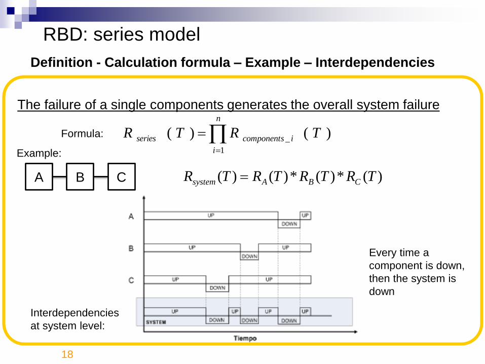
Definition - Calculation formula – Example – Interdependencies

A B C

RBD: series model

)()(1

_ TRTRn

i

icomponentsseries

)(*)(*)()( TRTRTRTR CBAsystem

Example:

The failure of a single components generates the overall system failure

Formula:

Interdependencies

at system level:

18

Every time a

component is down,

then the system is

down

A

B

C

RBD: parallel, total redundancy model

))(1(1)(1

__ TRTRn

i

icomponentredundancyotalparallel,t

)))(1(*))(1(*))(1((1)( TRTRTRTR CBAsystem Example:


Formula:

The system is up, if at least one single component is up

Interdependencies

at system level:

19

Every time a

component is up,

the system is up

20

RBD: parallel, partial redundancy model

iRR

RRj

nTR

componenticomponent

n

kj

jn

component

j

componentof_nk_outS

; with

)1()(

_

_,

where:


Interdependencies

at system level:

The system is a parallel model of n components, but it requires al least k

components over n for working

Formula:

Only if k

components over n

are down, then the

system is down

21

A

B

C

RBD: parallel, partial redundancy model

3

2

3

3_2, )1(3

)(j

j

component

j

componentof__outS RRj

TR

32333232

3_2, )1(*3)1(*3

3)1(*

2

3)( RRRRRRRTR of__outS


The system is a parallel model of n components, but it requires al least k

components over n for working

Example: Ra = Rb = Rc = R = 0,8 (case of

components with same reliability)

Multi-state system (MSS) logic -> system model with multi-states

• an extension to the traditional RBD parallel model:

• it enables to model a component unit / a subsystem working at different states

(rather than only at the two states of working and fault) corresponding to different

performance levels / rates;

• an impact factor is adopted, to express the reduction with respect to the nominal

performance level / rate of the subsystem, when a component fails.

E.g. 2 machines, the former having an impact factor, when it fails, equal to 25 % of the

nominal performance rate of the subsystem, the latter with an impact factor, when it

fails, equal to 75 %.

RBD: parallel, fractioning model

22

The reliability of a “series” system is always lower than the reliability of the

less reliable system component.

E.g., with 4 installed pumps:

R series (T) = 0,7 * 0,8 * 0,8 * 0,9= 0,403 = 40,3 % < 0,7 =

= min R A(T), R B(T), R C(T), R D(T)

The reliability of a “series” system is a decreasing function of the number

of system components.

If we consider only 3 pumps (A, B, C) instead of 4, we have:

R series (T) = R A(T) R B(T) R C(T) = 0,7*0,8*0,8 = 0,448 = 44,8 % >

R series (T) = R A(T) R B(T) R C(T) R D(T) = 0,7*0,8*0,8*0,9= 0,403 = 40,3

%

Properties of series systems

23

The reliability of a total “redundancy parallel system” is higher than the

reliability of the most reliable system component.

In case of parallel “1 out of 3”:

R parallel, total redundancy (T) = 1- (1-0,7)*(1-0,8)*(1-0,9) = 0,994 = 99,4 % >

0,9 = max R A(T), R B(T), R C(T)

The reliability of a total “redundancy parallel system” is an increasing

function of the number of system components.

Adding a pump (D) with R D(T) = 0,8, we have:

R parallel, total redundancy (T) = 1- (1-0,7) * (1-0,8) * (1-0,8) * (1-0,9) = 0,9988

= = 99,88 % >

R parallel, total redundancy (T) = 1- (1-0,7) * (1-0,8) * (1-0,9) = 0,994 = 99,4 %

Properties of parallel systems

24

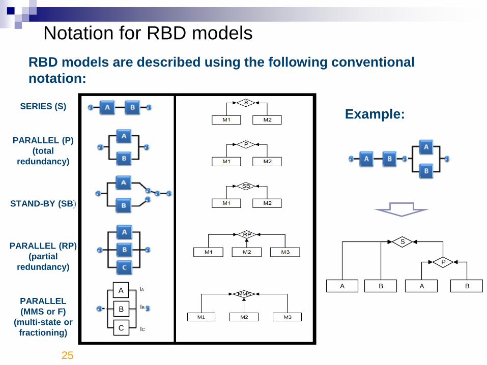
RBD models are described using the following conventional

notation:

A B

P

A B

S

Notation for RBD models

Example:SERIES (S)

PARALLEL (P)

(total

redundancy)

STAND-BY (SB)

PARALLEL (RP)

(partial

redundancy)

PARALLEL

(MMS or F)

(multi-state or

fractioning)

A B

P

A B

S

SERIES

PARALLEL

STAND-BY

PARTIAL REDUNDANCY

MULTI-STATE SYSTEM

M1 M2

MMS

M3

A

B

C

IA

IB

IC

25

Performance measure

For each production station, an Operating (working) Time can be calculated,

needed to complete the work order / the campaign. OT too is defined for each

planned operation in the production cycle.

Components:

ORmax maximum Output Rate of a given production station.

WC Work Content (of a “work order”).

ORmax expresses the (working) hours / days provided by a station to perform the

requested work order (i.e. it is maximum because it is defined under the

hypothesis of perfect workstation efficiency, without performance losses).

Therefore, the OT expresses how many working hours /days the workstation is

busy, under the hypothesis that it works at its maximum capacity.26

maxOR

WCOT

Definition – Operating Time

Reparto i

Reparto i+1

Tempo t

Reparto

t op precedente t op corrente

TTP

• L’ordine di produzione attraversa 2 reparti

• Il TTP è misurato per ciascun reparto i-esimo

• Il TTP di reparto misura il tempo trascorso dall’istante

di uscita dal reparto precedente fino all’istante di uscita

dal reparto corrente

Ordine in stato di attesa

Ordine in stato di lavoro

OT

TTP

Order in WAITING STATE

Order in WORKING STATE

TIME

SHOP 1

SHOP 2

SHOP

End previous op End current op

27

Performance measure

For each area / phase of the production system, a (working) equivalent Operating

time may be calculated, to complete the work order / the campaign (this too is

defined for each operation planned in the production cycle).

Components:

S is the number of workstations working in parallel in the same area / phase.

Definition – equivalent

Operating Time (1)

max

.ORS

WCOTeq

28

Area i Area i+1

Production

stream

Area i Area i+1

Production

stream

OT of station1 OT of station

2

OTeq phase 1 OTeq phase 2

OT of each workstation OT of each phase

With or

without inter-

operational

buffer

With or

without inter-

operational

buffer

Definition – equivalent

Operating Time (2)

TH of a workstation TH of a production phase

For a rough analysis (both nominal and effective value)

- TH phase i = Sum TH station j in phase / area i

To analyse reliability / availability of system

- it is needed to analyze the system in a logical-functional analysis (RBD scheme)

29

TH phase 1 = TH1 TH phase 2 = TH2Arrival rate

= TH0

Performance measure

Each area of the production system has a typical production capacity (also called

throughput); the nominal value of this capacity is, under the hypothesis of perfect

efficiency:

The maximum capacity of the production system is given by the bottleneck area /

phase (i.e., the area / phase with maximum OTeq, alias minimum TH).

With or

without inter-

operational

buffer

Nominal Throughput analysis (1)

i

ii

ieq

iWC

ORS

OTTH

max,

.,

1

30

UT phase 1 = UT1 UT phase 2 = UT2

Performance measure

From the analysis of the production capacity (throughput), it is possible to

calculate directly the level of utilization of the different areas / phases of the

production system.

Arrival rate

= TH0

Nominal Throughput analysis (2)

i

ii

ieqi

ieq

iTH

TH

OT

OTUT

min

max .,

.,

With or

without inter-

operational

buffer

performance analysis of production systems methods for

Documents