1

Performance Analysis of the NGST “Yardstick”Concept via Integrated Modeling

Gary Mosier, Keith Parrish, Michael FemianoNASA Goddard Space Flight Center

David Redding, Andrew Kissil, Miltiadis PapalexandrisJet Propulsion Laboratory

Larry Craig, Tim Page, Richard ShunkNASA Marshall Space Flight Center

August 2000

2

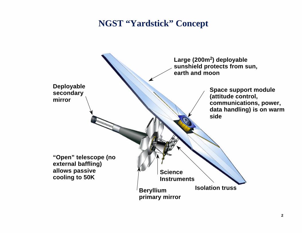
NGST “Yardstick” Concept

“Open” telescope (no external baffling) allows passive cooling to 50K

Deployable secondarymirror

Berylliumprimary mirror

Space support module (attitude control, communications, power, data handling) is on warm side

ScienceInstruments

Large (200m2) deployable sunshield protects from sun, earth and moon

Isolation truss

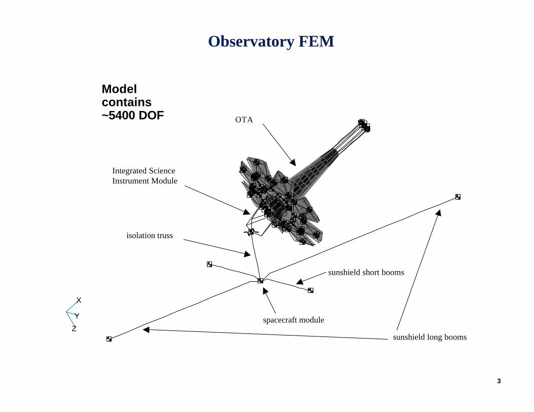
3

X

Y Z

sunshield long booms

sunshield short booms

Integrated Science Instrument Module

spacecraft module

isolation truss

OTA

Observatory FEM

Model contains ~5400 DOF

4

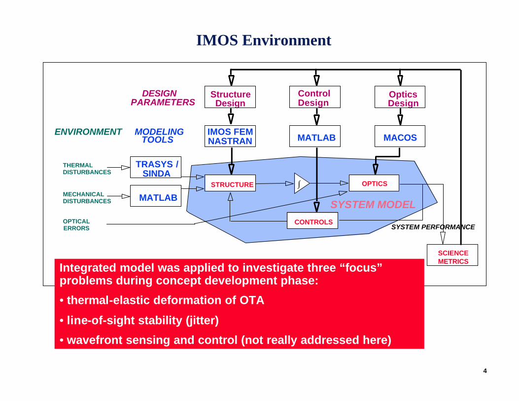
IMOS Environment

DESIGNPARAMETERS

MODELINGTOOLS

SYSTEM MODEL

THERMALDISTURBANCES

MECHANICALDISTURBANCES

ControlDesign

StructureDesign

OpticsDesign

MATLABIMOS FEMNASTRAN

STRUCTURE

CONTROLS

OPTICS

SCIENCEMETRICS

TRASYS /SINDA

SYSTEM PERFORMANCE

MATLAB

ENVIRONMENT

OPTICALERRORS

∫

MACOS

Integrated model was applied to investigate three “focus” problems during concept development phase:

• thermal-elastic deformation of OTA

• line-of-sight stability (jitter)

• wavefront sensing and control (not really addressed here)

5

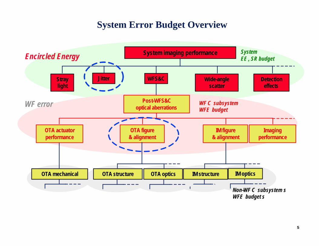
System Error Budget Overview

System imaging performance

Straylight

Wide-anglescatter

Detectioneffects

Jitter

Post-WFS&Coptical aberrations

OTA figure& alignment

IM figure& alignment

OTA actuatorperformance

Imagingperformance

OTA structure OTA optics IM structure IM opticsOTA mechanical

Encircled Energy

WF error

WFS&C

WF C subsystemWFE budget

SystemEE , SR budget

Non-WF C subsystem s WFE budget s

6

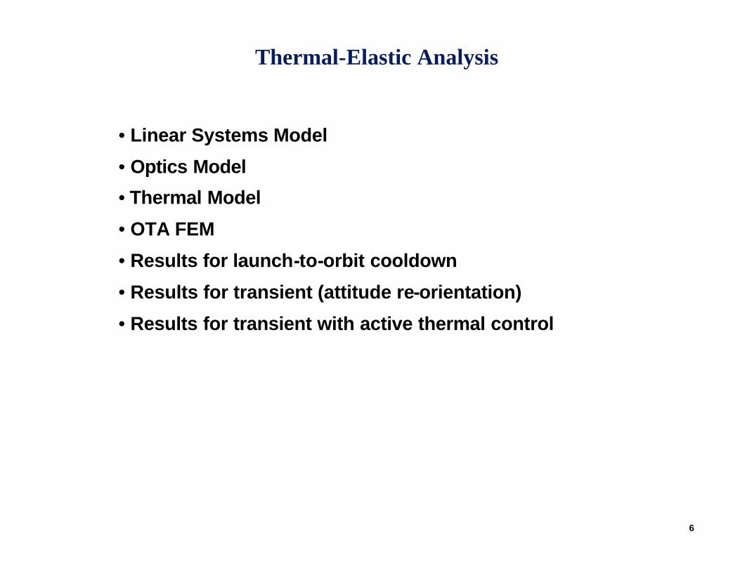
Thermal-Elastic Analysis

• Linear Systems Model

• Optics Model

• Thermal Model

• OTA FEM

• Results for launch-to-orbit cooldown

• Results for transient (attitude re-orientation)

• Results for transient with active thermal control

7

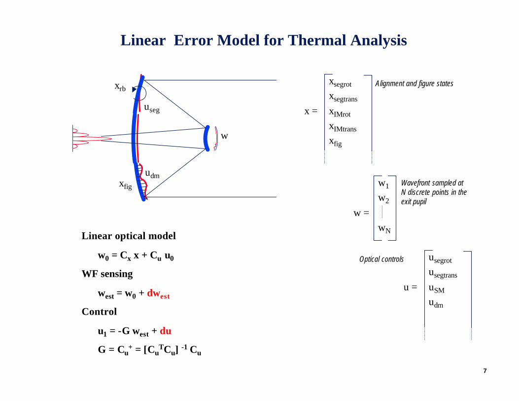
Linear Error Model for Thermal Analysis

Linear optical model

w0 = Cx x + Cu u0

WF sensing

west = w0 + dwest

Control

u1 = -G west + du

G = Cu+ = [Cu

TCu] -1 Cu

w

xrb

xfig

udm

useg x =

xsegrot

xsegtrans

xIMrot

xIMtrans

xfig

u =

usegrot

usegtrans

uSM

udm

w =

w1

w2

wN

Alignment and figure states

Wavefront sampled atN discrete points in theexit pupil

Optical controls

8

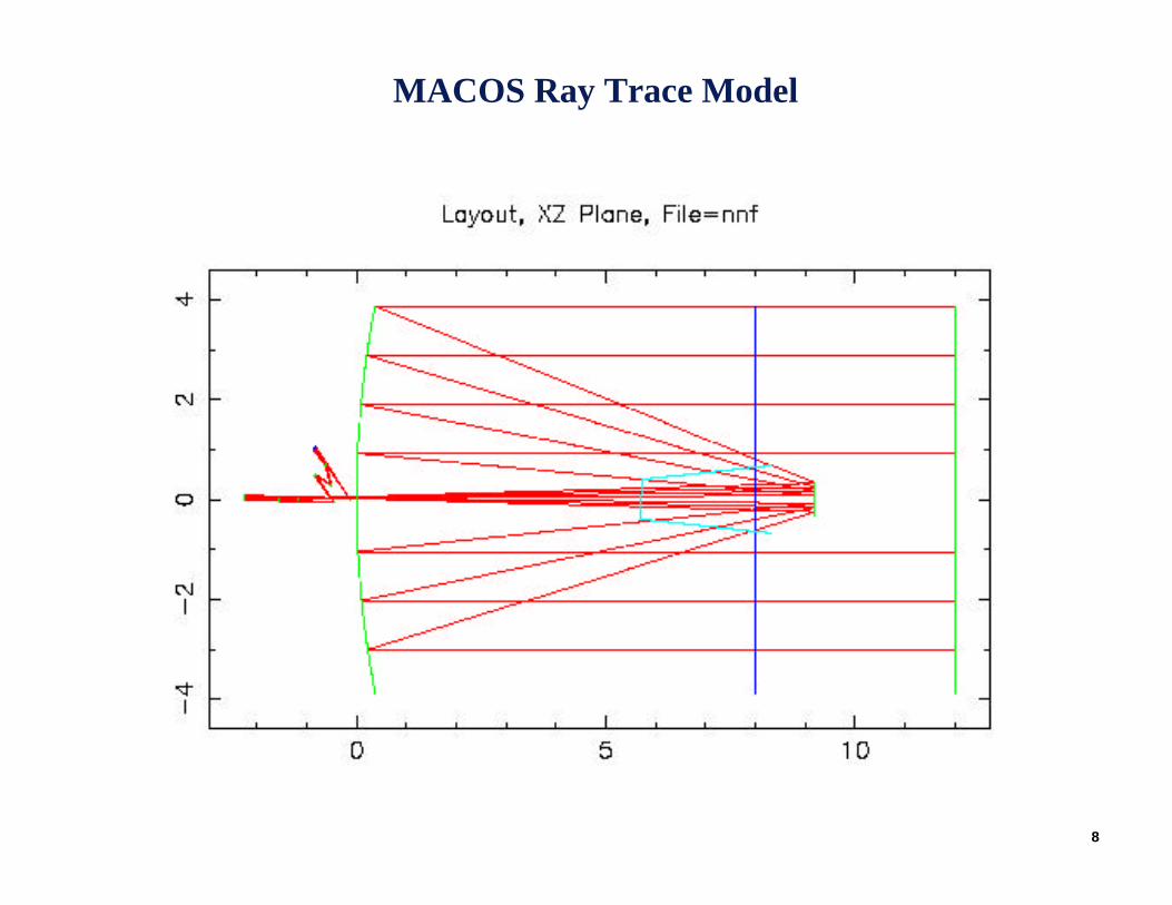
MACOS Ray Trace Model

9

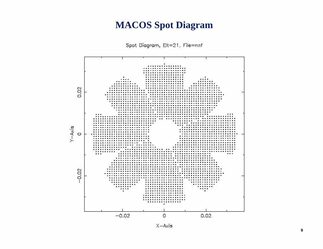
MACOS Spot Diagram

10

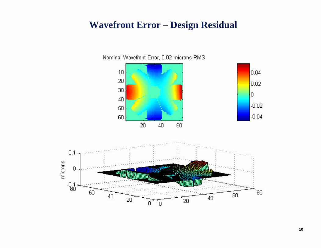
Wavefront Error – Design Residual

11

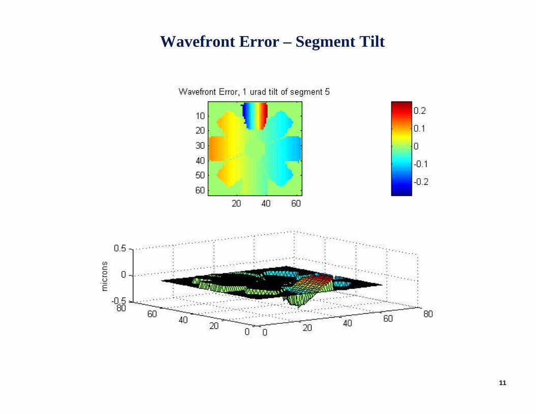
Wavefront Error – Segment Tilt

12

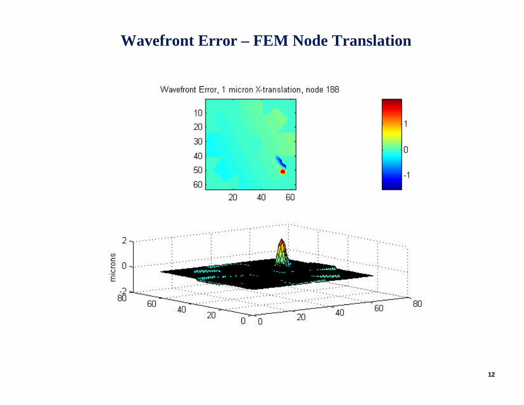
Wavefront Error – FEM Node Translation

13

X

Y

Z

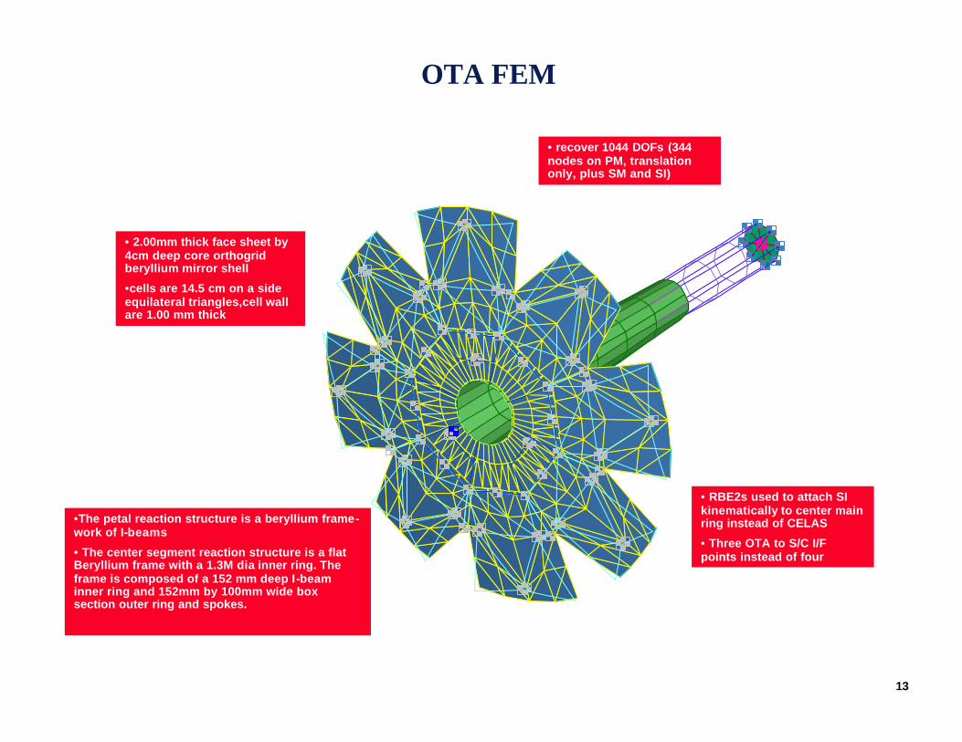
OTA FEM

• 2.00mm thick face sheet by 4cm deep core orthogridberyllium mirror shell

•cells are 14.5 cm on a side equilateral triangles,cell wall are 1.00 mm thick

• RBE2s used to attach SIkinematically to center main ring instead of CELAS

• Three OTA to S/C I/F points instead of four

•The petal reaction structure is a beryllium frame-work of I-beams

• The center segment reaction structure is a flat Beryllium frame with a 1.3M dia inner ring. The frame is composed of a 152 mm deep I-beam inner ring and 152mm by 100mm wide box section outer ring and spokes.

• recover 1044 DOFs (344 nodes on PM, translation only, plus SM and SI)

14

Observatory Thermal Model – Steady State

15

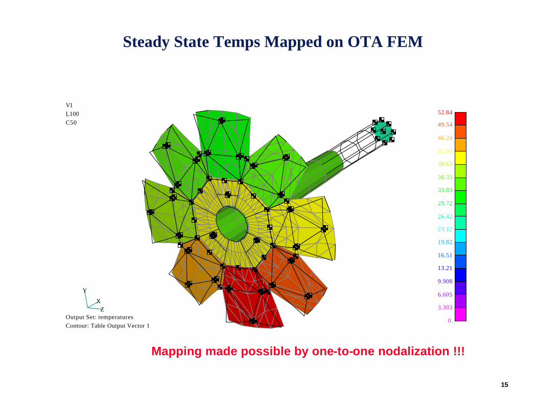
Steady State Temps Mapped on OTA FEM

X

Y

Z

52.84

49.54

46.24

42.93

39.63

36.33

33.03

29.72

26.42

23.12

19.82

16.51

13.21

9.908

6.605

3.303

0.

V1L100C50

Output Set: temperaturesContour: Table Output Vector 1

Mapping made possible by one-to-one nodalization !!!

16

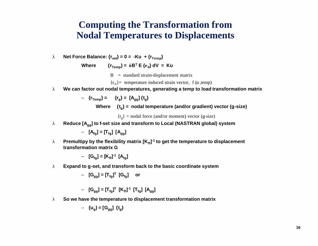
Computing the Transformation from Nodal Temperatures to Displacements

λ Net Force Balance: {rnet} = 0 = -Ku + {rTemp}

Where {rTemp} = ∫ BT E {ε 0} dV = Ku

B = standard strain-displacement matrix{ε0}= temperature induced strain vector, f (α,temp)

λ We can factor out nodal temperatures, generating a temp to load transformation matrix

– {rTemp} = {rg} = [Agg] {tg}

Where {tg} = nodal temperature (and/or gradient) vector (g-size)

{rg} = nodal force (and/or moment) vector (g-size)λ Reduce [Agg] to f-set size and transform to Local (NASTRAN global) system

– [Afg] = [Tfg] [Agg]

λ Premultipy by the flexibility matrix [Kff]-1 to get the temperature to displacement transformation matrix G

– [Gfg] = [Kff]-1 [Afg]

λ Expand to g-set, and transform back to the basic coordinate system

– [Ggg] = [Tfg]T [Gfg] or

– [Ggg] = [Tfg]T [Kff]-1 [Tfg] [Agg]

λ So we have the temperature to displacement transformation matrix

– {ug} = [Ggg] {tg}

17

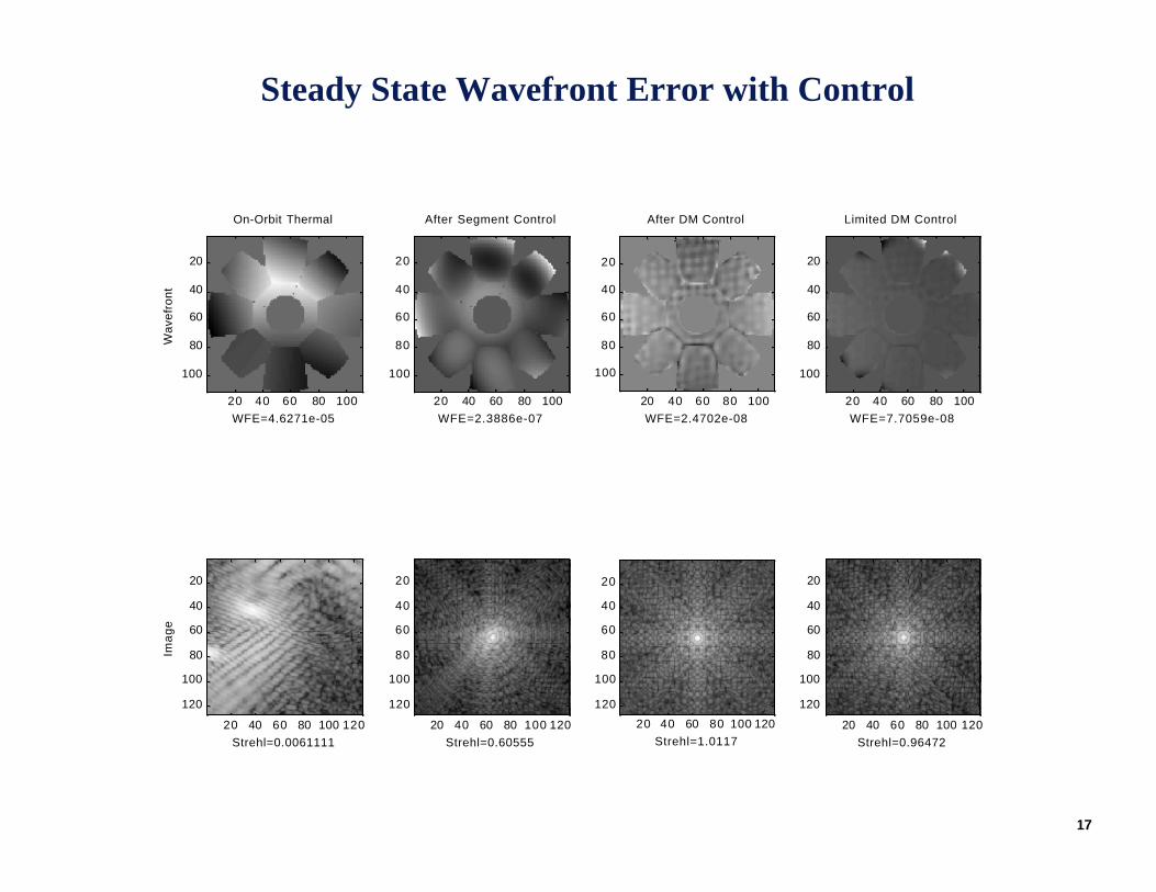
Steady State Wavefront Error with Control

On-Orbit Thermal

Wav

efro

nt

WFE=4.6271e-0520 40 60 80 100

20

40

60

80

100

Ima

ge

Strehl=0.006111120 40 60 80 100 120

20

40

60

80

100

120

After Segment Control

WFE=2.3886e-0720 40 60 80 100

20

40

60

80

100

Strehl=0.6055520 40 60 80 100 120

20

40

60

80

100

120

After DM Control

WFE=2.4702e-0820 40 60 80 100

20

40

60

80

100

Strehl=1.011720 40 60 80 100 120

20

40

60

80

100

120

Limited DM Control

WFE=7.7059e-0820 40 60 80 100

20

40

60

80

100

Strehl=0.9647220 40 60 80 100 120

20

40

60

80

100

120

18

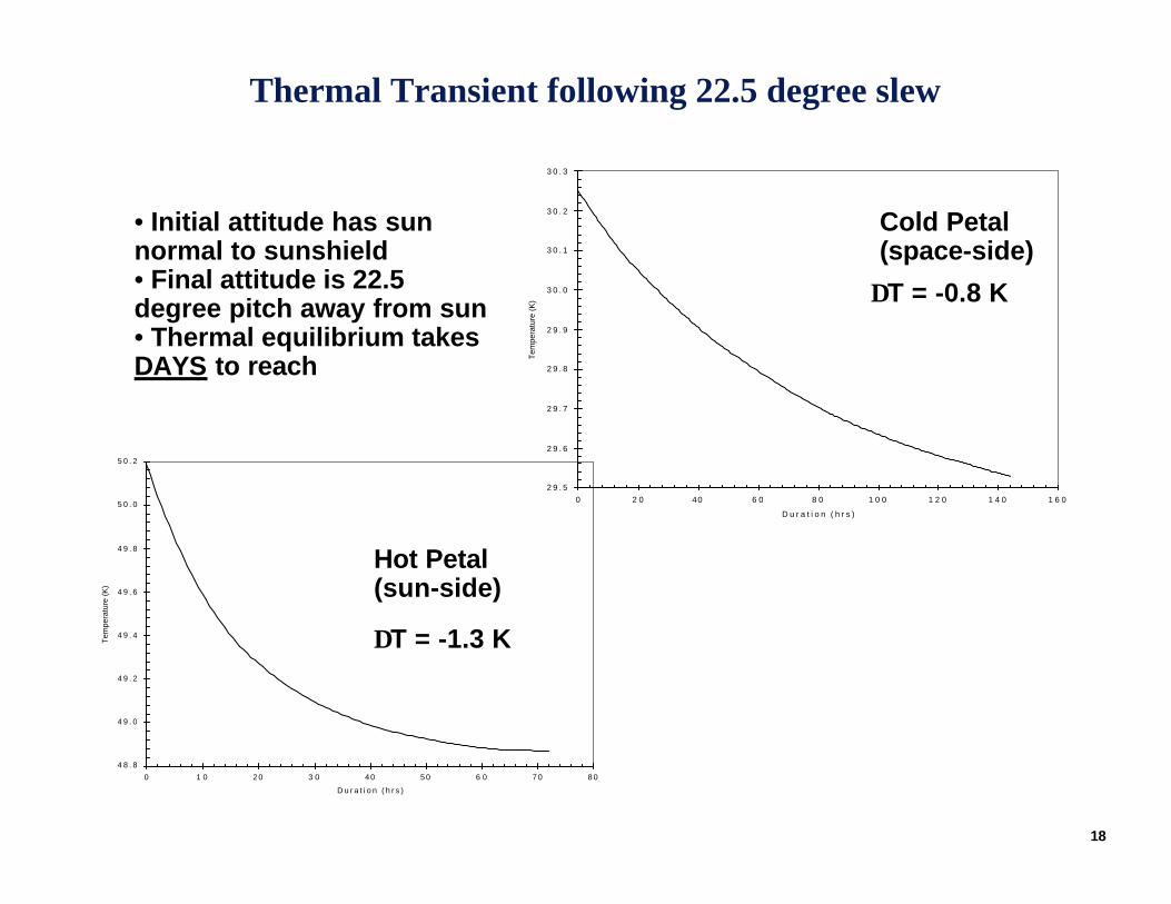
Thermal Transient following 22.5 degree slew

4 8 . 8

4 9 . 0

4 9 . 2

4 9 . 4

4 9 . 6

4 9 . 8

5 0 . 0

5 0 . 2

0 1 0 2 0 3 0 4 0 5 0 6 0 7 0 8 0

D u r a t i o n ( h r s )

Tem

pera

ture

(K

)

2 9 . 5

2 9 . 6

2 9 . 7

2 9 . 8

2 9 . 9

3 0 . 0

3 0 . 1

3 0 . 2

3 0 . 3

0 2 0 40 6 0 8 0 1 0 0 1 2 0 1 4 0 1 6 0

D u r a t i o n ( h r s )

Tem

pera

ture

(K)

Cold Petal(space-side)

Hot Petal(sun-side)

∆T = -0.8 K

∆T = -1.3 K

• Initial attitude has sun normal to sunshield• Final attitude is 22.5 degree pitch away from sun• Thermal equilibrium takes DAYS to reach

19

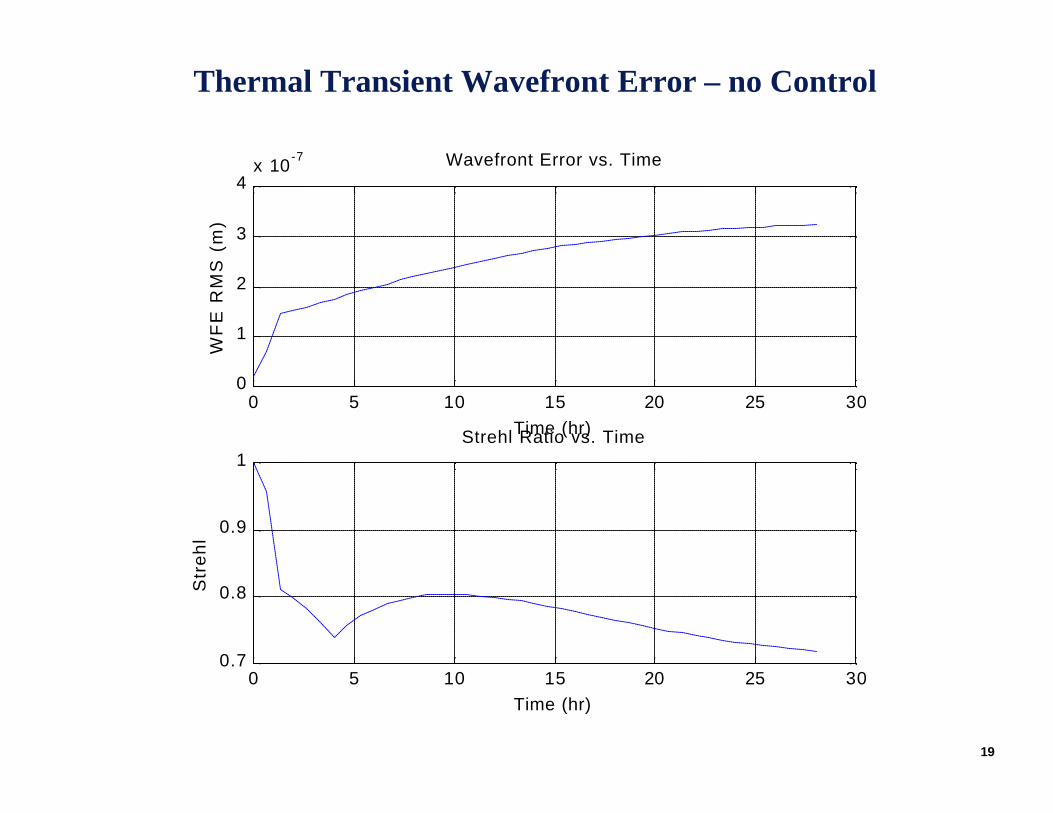
Thermal Transient Wavefront Error – no Control

0 5 10 15 20 25 300

1

2

3

4x 10

-7 Wavefront Error vs. Time

Time (hr)

WF

E R

MS

(m

)

0 5 10 15 20 25 300.7

0.8

0.9

1Strehl Ratio vs. Time

Time (hr)

Str

eh

l

20

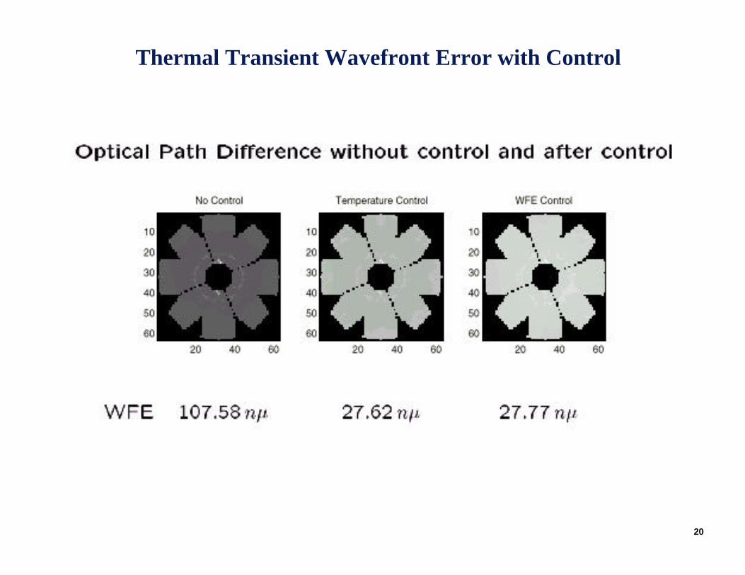
Thermal Transient Wavefront Error with Control

21

Jitter Analysis

• Pointing Control Architecture

• Linear Systems Model

• Disturbance Model

• Compensation Model

• Results for parametric studies

22

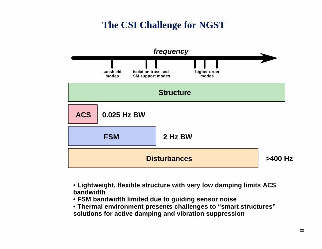
The CSI Challenge for NGST

frequency

ACS 0.025 Hz BW

Disturbances >400 Hz

FSM 2 Hz BW

Structure

sunshieldmodes

isolation truss andSM support modes

higher ordermodes

• Lightweight, flexible structure with very low damping limits ACS bandwidth• FSM bandwidth limited due to guiding sensor noise• Thermal environment presents challenges to “smart structures” solutions for active damping and vibration suppression

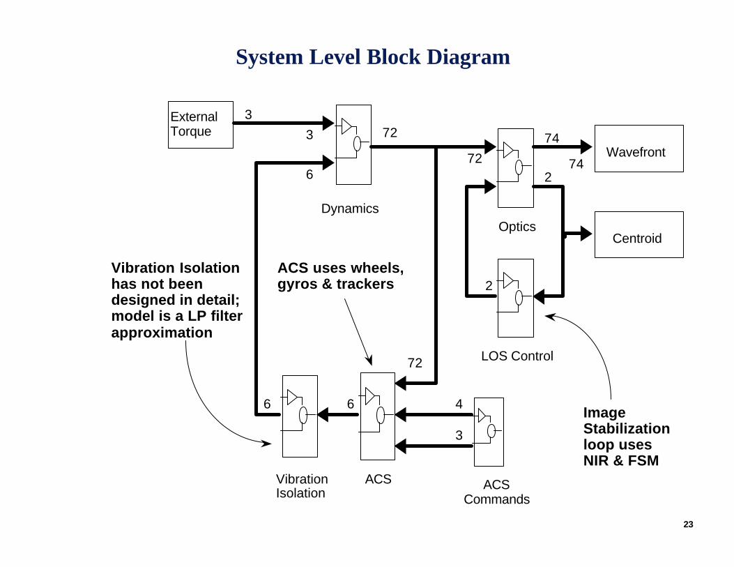
23

System Level Block Diagram

Optics

Wavefront

LOS Control

ExternalTorque

Dynamics

Centroid

ACSCommands

ACS

6 4

3

74

74

2

72

72

72

6

6

3

3

2

VibrationIsolation

ACS uses wheels,gyros & trackers

ImageStabilizationloop usesNIR & FSM

Vibration Isolationhas not beendesigned in detail;model is a LP filterapproximation

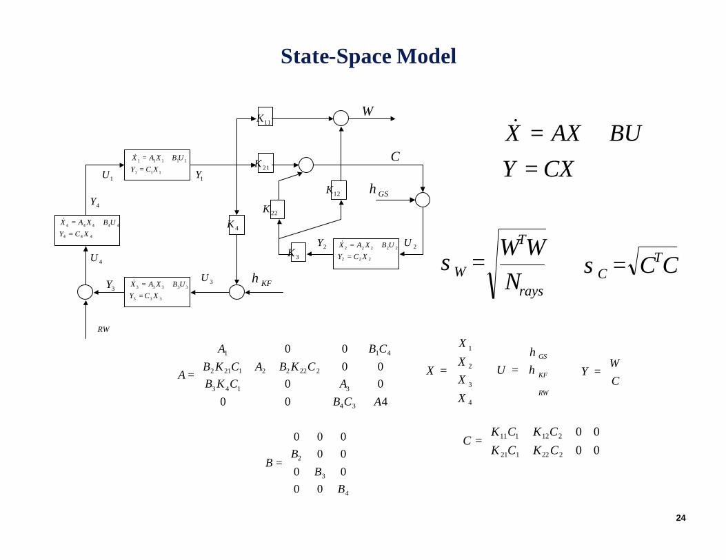
24

State-Space Model

111

11111

XCY

UBXAX

=

+=&

222

22222

XCY

UBXAX

=

+=&

333

33333

XCY

UBXAX

=

+=&

444

44444

XCY

UBXAX

=

+=&

1U

KFη++

+

GSη

RWℑ

W

C

2U

3U

4U2Y

1Y

3Y

4Y

+

+

4K

11K

12K

22K

21K

3K

+

+

+

++

CXYBUAXX

=+=&

ℑ

=

RW

KF

GS

U ηη

=

4

3

2

1

X

XX

X

X

=

CW

Y

+

=

4000000

00

34

3143

222221212

411

ACBACKB

CKBACKBCBA

A

=

4

3

2

0000

00000

BB

BB

=

0000

222121

212111

CKCKCKCK

C

rays

T

W NWW

=σ CCTC =σ

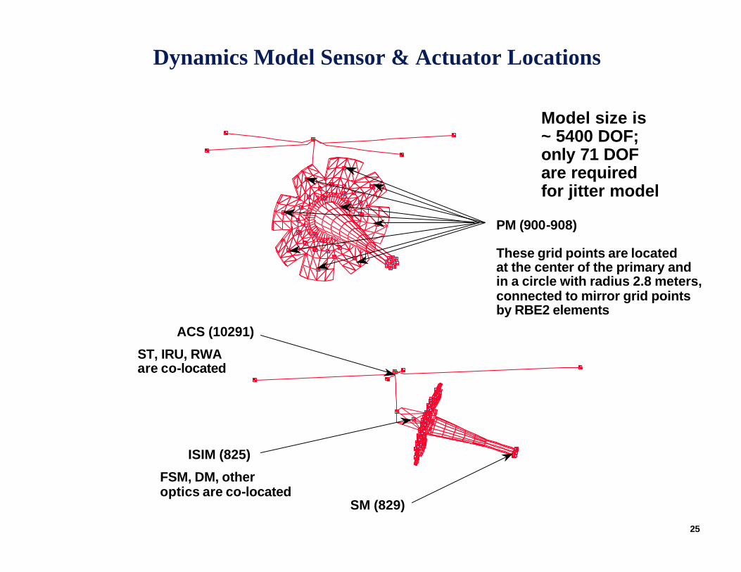
25

Dynamics Model Sensor & Actuator Locations

ACS (10291)

ISIM (825)

SM (829)

PM (900-908)

These grid points are locatedat the center of the primary andin a circle with radius 2.8 meters,connected to mirror grid pointsby RBE2 elements

ST, IRU, RWAare co-located

FSM, DM, otheroptics are co-located

Model size is~ 5400 DOF;only 71 DOFare requiredfor jitter model

26

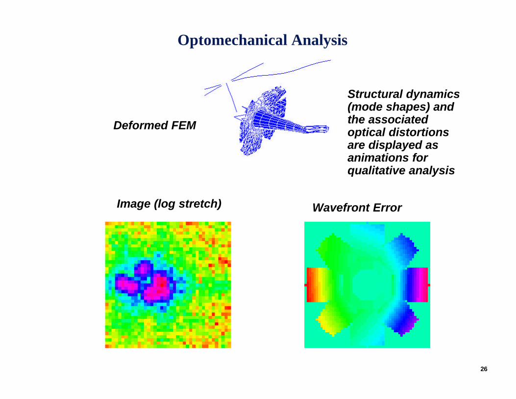
Optomechanical Analysis

Structural dynamics(mode shapes) andthe associatedoptical distortionsare displayed asanimations forqualitative analysis

Image (log stretch) Wavefront Error

Deformed FEM

27

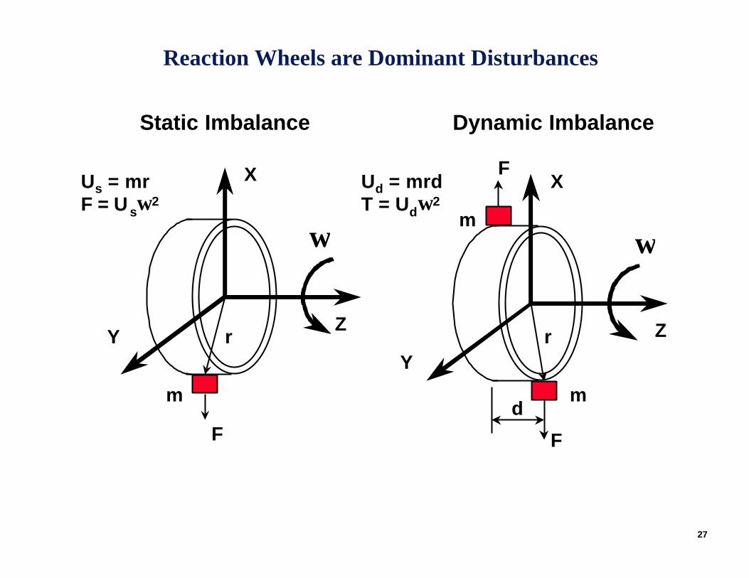
Reaction Wheels are Dominant Disturbances

Static Imbalance Dynamic Imbalance

ω

F

F

d

r

m

mω

F

r

m

Us = mrF = U sω2

Ud = mrdT = Udω2

YZ

X X

Y

Z

28

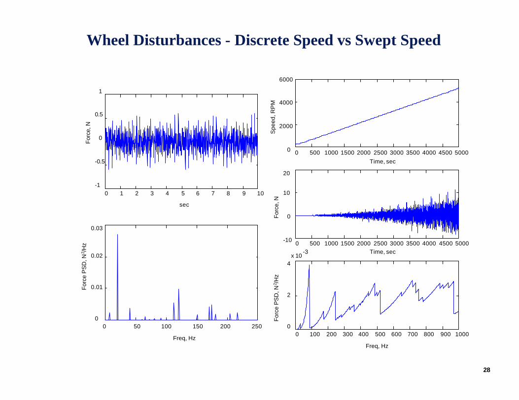
Wheel Disturbances - Discrete Speed vs Swept Speed

0 1 2 3 4 5 6 7 8 9 10-1

-0.5

0

0.5

1

sec

Forc

e, N

0 50 100 150 200 2500

0.01

0.02

0.03

Freq, Hz

For

ce P

SD

, N2 /

Hz

0 500 1000 1500 2000 2500 3000 3500 4000 4500 50000

2000

4000

6000

Time, sec

Spe

ed, R

PM

0 500 1000 1500 2000 2500 3000 3500 4000 4500 5000-10

0

10

20

Time, sec

Forc

e, N

0 100 200 300 400 500 600 700 800 900 10000

2

4x 10

-3

Freq, Hz

For

ce P

SD

, N2 /

Hz

29

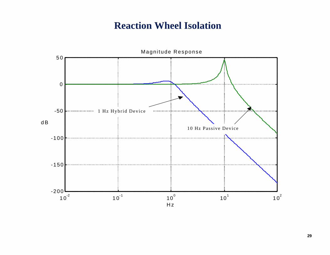
Reaction Wheel Isolation

1 0-2

1 0-1

100

101

1 02

-200

-150

-100

-50

0

5 0

d B

H z

Magn i tude Response

1 Hz Hybr id Dev ice

10 Hz Pass ive Device

30

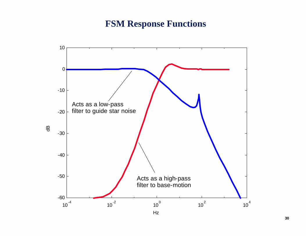
FSM Response Functions

10-4

10-2

100

102

104

-60

-50

-40

-30

-20

-10

0

10

Hz

dB

Acts as a high-passfilter to base-motion

Acts as a low-passfilter to guide star noise

31

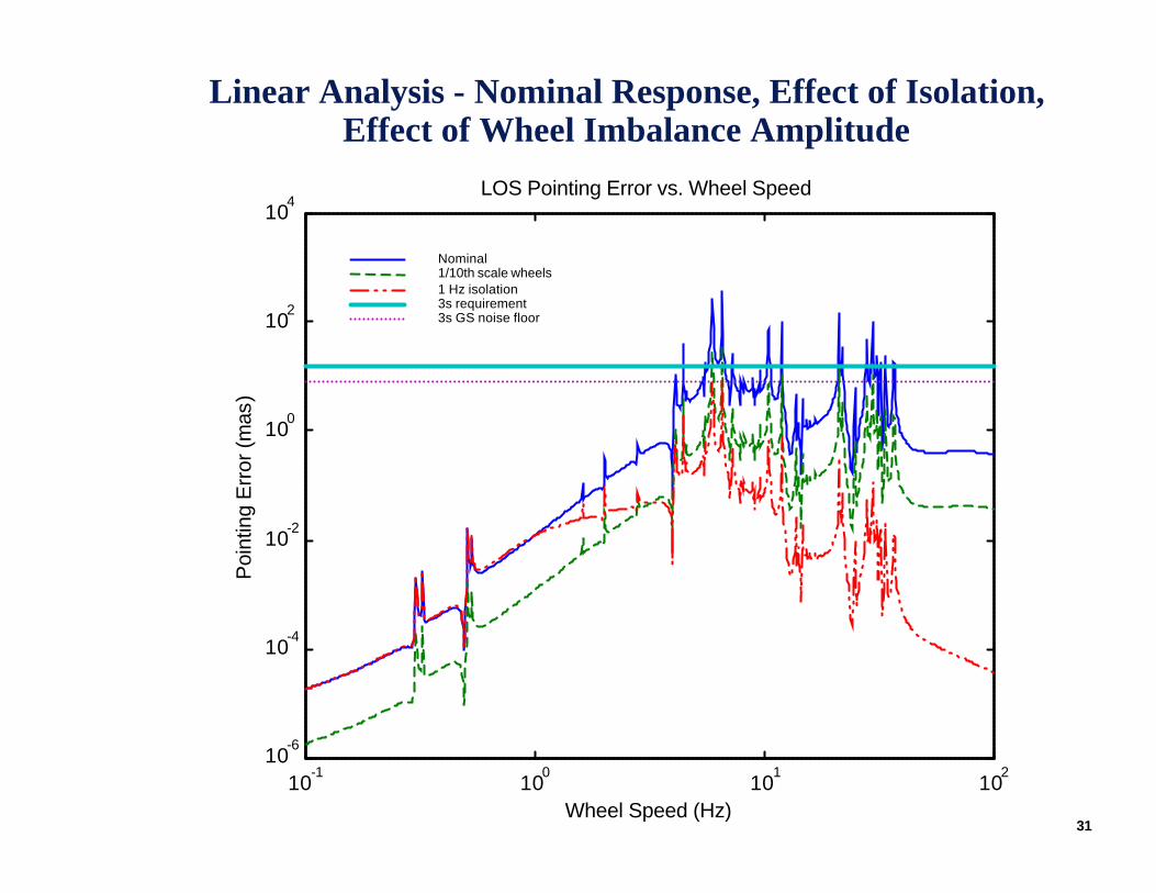
Linear Analysis - Nominal Response, Effect of Isolation, Effect of Wheel Imbalance Amplitude

10-1

100

101

102

10-6

10-4

10-2

100

102

104

Wheel Speed (Hz)

Poi

ntin

g E

rror

(mas

)

LOS Pointing Error vs. Wheel Speed

Nominal1/10th scale wheels1 Hz isolation3s requirement3s GS noise floor

32

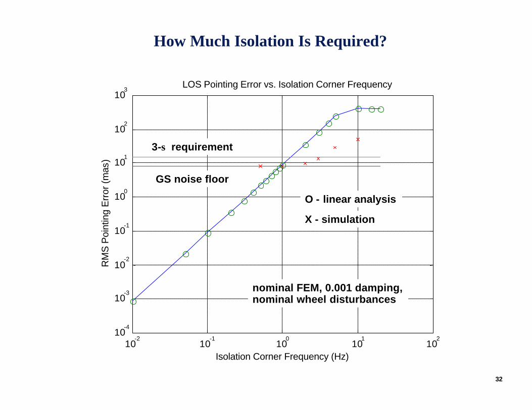
How Much Isolation Is Required?

10-2

10-1

100

101

102

10-4

10-3

10-2

10-1

100

101

102

103

Isolation Corner Frequency (Hz)

RM

S P

oint

ing

Err

or (m

as)

LOS Pointing Error vs. Isolation Corner Frequency

O - linear analysis

3-σ requirement

X - simulation

GS noise floor

nominal FEM, 0.001 damping,nominal wheel disturbances

33

Conclusions

• Development of end-to-end models using the IMOS environment was relatively painless, owing to the following factors:

• translation from NASTRAN and SINDA was possible for FEM and TMM, as was output to FEMAP neutral format

• geometric and material properties were easily parameterized, as were all other significant entities in the models

• ray-trace code (MACOS) was open-source, so it could be integrated via Mex-function API

• Matlab™ is a matrix-oriented language/tool, with integrated graphics and visualization

• Questions remain about the ability to handle realistically-sized models within Matlab™ (eigenvalues, matrix inversion)

• None of these models have been validated, of course…