UNIVERSITE DE MONTREAL

PERFORMANCE EVALUATION AND ANALYSIS OF MIMO SCHEMES IN LTE

NETWORKS ENVIRONMENT

ALI JEMMALI

DEPARTEMENT DE GENIE ELECTRIQUE

ECOLE POLYTECHNIQUE DE MONTREAL

THESE PRESENTEE EN VUE DE L’OBTENTION

DU DIPLOME DE PHILOSOPHIÆ DOCTOR

(GENIE ELECTRIQUE)

DECEMBRE 2013

c© Ali Jemmali, 2013.

UNIVERSITE DE MONTREAL

ECOLE POLYTECHNIQUE DE MONTREAL

Cette these intitulee :

PERFORMANCE EVALUATION AND ANALYSIS OF MIMO SCHEMES IN LTE

NETWORKS ENVIRONMENT

presentee par : JEMMALI Ali

en vue de l’obtention du diplome de : Philosophiæ Doctor

a ete dument acceptee par le jury d’examen constitue de :

M. CARDINAL Christian, Ph.D., president

M. CONAN Jean, Ph.D., membre et directeur de recherche

M. WU Ke, Ph.D., membre et codirecteur de recherche

M. AKYEL Cevdet, D.Sc.A, membre

M. AJIB Wessam, Ph.D., membre

iii

To my dear mother, my dear wife and dear son,

In memory of my father. . .

iv

ACKNOWLEDGEMENTS

I would like to express the deepest appreciation to my director of research, Dr Jean Co-

nan and my co-director of research, Dr Ke Wu. My sincere gratitude goes to my director

of research for his continuous support of my Ph.D study and research, for his motivation,

enthusiasm and immense knowledge. His guidance helped me in all the time of research and

writing of this thesis. I also wish to express my truthful recognition to Dr Ke Wu for his

continuous encouragement and support. Without the support, encouragement of my super-

visors, this thesis would not have been possible.

My sincere gratitude goes towards my thesis examiners :

– Prof. Cardinal Christian (Committee Chair), Dept. Electrical Engineering, Ecole Poly-

technique, Montreal,

– Prof. Ajib Wessam (External Examiner), Dept. Computer Science, UQAM, Montreal,

– Prof. Cevdet Akyel, Dept. Electrical Engineering, Ecole Polytechnique, Montreal,

for accepting reviewing my work and for their valuable comments towards the impro-

vement of my final thesis report, as well as putting me through a stimulating, albeit a bit

stressful, defense experience.

Special thanks go also go to my student colleagues in the laboratory for the technical

exchanges and fruitful discussions. I mention for memory Wael, Jihed and Tarek. My truth-

ful recognition goes to Mohammad Torabi for his precious help and advises. Big thanks also

goes to my colleagues, namely Vladan Jevromovic and Benoit Courchesne for their encourage-

ment and for giving me one day off for more than one year to help me finalize my thesis work.

Last but not least, I would like to thank my dear wife for her patience, support and

sacrifice.

v

RESUME

Dans cette these, nous proposons d’evaluer et d’analyser les performances des configu-

rations radio a antennes multiples a l’emission et/ou la reception (MIMO) dans l’environ-

nement des reseaux LTE (Long Term Evolution). Plus specifiquement, on s’interesse a la

couche physique de l’interface radio OFDM-MIMO de ces reseaux. Apres une introduction

rapide aux reseaux LTE et aux techniques MIMO, on presente dans une premiere etape, une

analyse theorique du taux d’erreur binaire en fonction du rapport signal sur bruit des deux

principaux codes spatio-temporels de la norme LTE, a savoir le codage SFBC 2 × 1 (Space

Frequency Block Coding) et le codage FSTD 4 × 2 (Frequency Switch Transmit Diversity).

On developpe les equations analytiques du taux d’erreur binaire de ces codes dans un canal

a evanouissement de Rayleigh sans correlation spatiale qui sont par la suite comparees a des

valeurs obtenues par simulations Monte-Carlo. Dans une deuxieme etape, on considere l’eva-

luation de la capacite du canal resultant de l’utilisation de ces memes codes dans un canal a

evanouissement de Rayleigh. Pour fin de comparaison, on propose par la suite d’evaluer par

simulation leur debit effectif. Les resultats montrent que la capacite peut effectivement etre

presque atteinte en pratique. Le deuxieme volet de cette these considere les performances des

systemes MIMO utilisant la selection d’antennes. Nous utilisons la theorie d’ordre statistique

pour developper des equations analytiques relatives au taux d’erreur binaire des systemes

avec selection d’antennes du cote recepteur dans un canal d’evanouissement de Rayleigh sans

correlation spatiale. Afin de valider numeriquement les resultats de notre analyse, un algo-

rithme a selection d’antenne au recepteur a ete developpe et utilise en simulation. Dans un

dernier temps, on evalue l’effet de la correlation spatiale entre les antennes. L’etude est faite

a partir de simulations et d’un modele de correlation spatiale base sur le produit Kronecker

de deux matrices de correlation relatives respectivement a l’emission et a la reception.

vi

ABSTRACT

This thesis considers both an analysis and a numerical evaluation of the performance of

MIMO radio systems in the LTE network environment. More specifically we consider the

physical layer of the OFDM-MIMO based radio interface. As a first step we present a theo-

retical analysis of the bit error rate of the two space-time codes adopted by the LTE norm,

namely the SFBC 2× 1 and FSTD 4× 2 codes, as a function of the signal upon noise ratio.

Analytical expressions are given for transmission over a Rayleigh channel without spatial

correlation which are then compared with Monte-Carlo simulations. As a second step, we

consider the capacity of the channel obtained by using these codes on a Rayleigh fading

channel. Results show that simulated throughput almost reaches the capacity limit. As a

different topic, this thesis considers also MIMO systems based on antenna selection. By us-

ing order statistics we develop analytical expressions for the error rate on a Rayleigh channel

without antenna correlation. In order to validate our numerical results, an algorithm imple-

menting antenna selection at the receiver has been developed and used in the simulations.

As a last step the effect of antenna correlation is investigated through the use of simulations

and a model of spatial antenna correlation based on the Kronecker product of two correlation

matrices related to the transmitting and receiving elements of the MIMO scheme.

vii

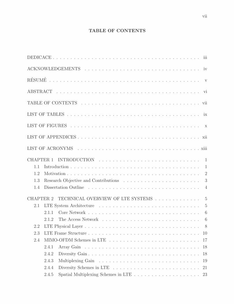
TABLE OF CONTENTS

DEDICACE . . . . . . . . . . . . . . . . . . . . . . . . . . . . . . . . . . . . . . . . . . iii

ACKNOWLEDGEMENTS . . . . . . . . . . . . . . . . . . . . . . . . . . . . . . . . . iv

RESUME . . . . . . . . . . . . . . . . . . . . . . . . . . . . . . . . . . . . . . . . . . . v

ABSTRACT . . . . . . . . . . . . . . . . . . . . . . . . . . . . . . . . . . . . . . . . . vi

TABLE OF CONTENTS . . . . . . . . . . . . . . . . . . . . . . . . . . . . . . . . . . vii

LIST OF TABLES . . . . . . . . . . . . . . . . . . . . . . . . . . . . . . . . . . . . . . ix

LIST OF FIGURES . . . . . . . . . . . . . . . . . . . . . . . . . . . . . . . . . . . . . x

LIST OF APPENDICES . . . . . . . . . . . . . . . . . . . . . . . . . . . . . . . . . . . xii

LIST OF ACRONYMS . . . . . . . . . . . . . . . . . . . . . . . . . . . . . . . . . . . xiii

CHAPTER 1 INTRODUCTION . . . . . . . . . . . . . . . . . . . . . . . . . . . . . 1

1.1 Introduction . . . . . . . . . . . . . . . . . . . . . . . . . . . . . . . . . . . . . 1

1.2 Motivation . . . . . . . . . . . . . . . . . . . . . . . . . . . . . . . . . . . . . . 2

1.3 Research Objective and Contributions . . . . . . . . . . . . . . . . . . . . . . 3

1.4 Dissertation Outline . . . . . . . . . . . . . . . . . . . . . . . . . . . . . . . . 4

CHAPTER 2 TECHNICAL OVERVIEW OF LTE SYSTEMS . . . . . . . . . . . . . 5

2.1 LTE System Architecture . . . . . . . . . . . . . . . . . . . . . . . . . . . . . 5

2.1.1 Core Network . . . . . . . . . . . . . . . . . . . . . . . . . . . . . . . . 6

2.1.2 The Access Network . . . . . . . . . . . . . . . . . . . . . . . . . . . . 6

2.2 LTE Physical Layer . . . . . . . . . . . . . . . . . . . . . . . . . . . . . . . . . 8

2.3 LTE Frame Structure . . . . . . . . . . . . . . . . . . . . . . . . . . . . . . . . 10

2.4 MIMO-OFDM Schemes in LTE . . . . . . . . . . . . . . . . . . . . . . . . . . 17

2.4.1 Array Gain . . . . . . . . . . . . . . . . . . . . . . . . . . . . . . . . . 18

2.4.2 Diversity Gain . . . . . . . . . . . . . . . . . . . . . . . . . . . . . . . . 18

2.4.3 Multiplexing Gain . . . . . . . . . . . . . . . . . . . . . . . . . . . . . 19

2.4.4 Diversity Schemes in LTE . . . . . . . . . . . . . . . . . . . . . . . . . 21

2.4.5 Spatial Multiplexing Schemes in LTE . . . . . . . . . . . . . . . . . . . 23

viii

CHAPTER 3 PERFORMANCE EVALUATION OF MIMO SYSTEMS IN LTE . . . 28

3.1 Introduction . . . . . . . . . . . . . . . . . . . . . . . . . . . . . . . . . . . . . 28

3.2 BER Analysis of LTE MIMO Schemes . . . . . . . . . . . . . . . . . . . . . . 30

3.2.1 System Model . . . . . . . . . . . . . . . . . . . . . . . . . . . . . . . . 30

3.2.2 Average BER Performance analysis for several M-QAM Schemes . . . . 30

3.2.3 Numerical results and discussions for the average BER . . . . . . . . . 34

3.3 Channel Capacity Analysis for LTE systems . . . . . . . . . . . . . . . . . . . 37

3.3.1 Channel Model and Channel Capacity of Spatial Multiplexing Scheme . 38

3.3.2 Channel Model and Channel Capacity of Diversity Schemes . . . . . . 39

3.4 Data Throughput Performance Evaluation for M-QAM Modulation Schemes . 44

3.4.1 Numerical Results and Discussion for System Throughput . . . . . . . 47

CHAPTER 4 ANTENNA SELECTION IN MIMO SYSTEMS . . . . . . . . . . . . . 52

4.1 Antenna Selection Overview . . . . . . . . . . . . . . . . . . . . . . . . . . . . 53

4.1.1 Antenna Selection Scheme based on the Channel Capacity . . . . . . . 56

4.1.2 Antenna Selection Scheme based on the SNR . . . . . . . . . . . . . . . 58

4.1.3 Antenna Selection Algorithms . . . . . . . . . . . . . . . . . . . . . . . 59

4.2 Performance Evaluation of UCBS Antenna Selection Algorithm . . . . . . . . 68

4.2.1 Impact of the UCBS Algorithm on the capacity of MIMO systems . . . 68

4.3 BER Analysis of the MIMO STBC System using Receive Antenna Selection . 70

4.3.1 Error analysis of the receive antenna selection scheme . . . . . . . . . . 71

4.4 Effect of Antenna Correlation on Receive Antenna Selection . . . . . . . . . . 75

4.4.1 System and Channel Model . . . . . . . . . . . . . . . . . . . . . . . . 76

4.4.2 Simulations Results and Discussion . . . . . . . . . . . . . . . . . . . . 77

CHAPTER 5 SUMMARY AND CONCLUSIONS . . . . . . . . . . . . . . . . . . . . 83

5.1 Future Work . . . . . . . . . . . . . . . . . . . . . . . . . . . . . . . . . . . . . 84

5.1.1 MU-MIMO Aspects . . . . . . . . . . . . . . . . . . . . . . . . . . . . . 84

5.1.2 CSI Aspects . . . . . . . . . . . . . . . . . . . . . . . . . . . . . . . . . 84

5.1.3 Frequency Selective Channel Aspects . . . . . . . . . . . . . . . . . . . 85

5.1.4 Antenna Correlated Channel Aspects . . . . . . . . . . . . . . . . . . . 85

5.1.5 Contributions and Publications . . . . . . . . . . . . . . . . . . . . . . 85

REFERENCES . . . . . . . . . . . . . . . . . . . . . . . . . . . . . . . . . . . . . . . . 87

APPENDICES . . . . . . . . . . . . . . . . . . . . . . . . . . . . . . . . . . . . . . . . 92

ix

LIST OF TABLES

Table 2.1 Resource Block as a function of Channel Bandwidth . . . . . . . . . . . 15

Table 2.2 Antenna ports and their associated Reference Signals . . . . . . . . . . 20

Table 2.3 Codewords-to-layer Mapping in LTE . . . . . . . . . . . . . . . . . . . 24

Table 2.4 Codewords for 2× 2 Open Loop Spatial Multiplexing . . . . . . . . . . 25

Table 2.5 Codewords for 4× 4 Open Loop Spatial Multiplexing . . . . . . . . . . 25

Table 3.1 Simulation Settings . . . . . . . . . . . . . . . . . . . . . . . . . . . . . 35

Table 3.2 Number of Resource Blocks . . . . . . . . . . . . . . . . . . . . . . . . 45

Table 3.3 ECR and Modulation Order for CQI . . . . . . . . . . . . . . . . . . . 46

Table 3.4 SISO Generated Data . . . . . . . . . . . . . . . . . . . . . . . . . . . 47

Table 4.1 UCBS Selection Algorithm . . . . . . . . . . . . . . . . . . . . . . . . 66

x

LIST OF FIGURES

Figure 2.1 LTE System Architecture. . . . . . . . . . . . . . . . . . . . . . . . . . 5

Figure 2.2 User Plan Protocols. . . . . . . . . . . . . . . . . . . . . . . . . . . . . 8

Figure 2.3 Control Plan Protocols. . . . . . . . . . . . . . . . . . . . . . . . . . . 8

Figure 2.4 LTE downlink Physical Layer Block Diagram. . . . . . . . . . . . . . . 9

Figure 2.5 Type 1 LTE FDD Frame Structure. . . . . . . . . . . . . . . . . . . . . 11

Figure 2.6 Type 2 LTE TDD Frame Structure. . . . . . . . . . . . . . . . . . . . . 11

Figure 2.7 Structure of the symbols in one slot with Normal Cyclic Prefix. . . . . 12

Figure 2.8 Structure of the symbols in one slot with Extended Cyclic Prefix. . . . 13

Figure 2.9 OFDM Signal Generation. . . . . . . . . . . . . . . . . . . . . . . . . . 14

Figure 2.10 LTE Resource Block. . . . . . . . . . . . . . . . . . . . . . . . . . . . . 15

Figure 2.11 Physical Channels and Physical Signals in LTE. . . . . . . . . . . . . . 16

Figure 2.12 Space Frequency Block Coding (SFBC) Scheme in LTE . . . . . . . . . 21

Figure 2.13 Frequency Switched Transmit Diversity (FSTD) Scheme in LTE . . . . 22

Figure 2.14 2× 2 Open Loop Spatial Multiplexing with Large-Delay CDD Precoding. 26

Figure 3.1 BER Results for QPSK Modulation . . . . . . . . . . . . . . . . . . . . 36

Figure 3.2 BER Results for 16-QAM Modulation . . . . . . . . . . . . . . . . . . 36

Figure 3.3 BER Results for 64-QAM Modulation . . . . . . . . . . . . . . . . . . 37

Figure 3.4 Capacity for SISO, SFBC-OFDM and FSTD-OFDM Schemes . . . . . 43

Figure 3.5 System Capacity as a function of SNR . . . . . . . . . . . . . . . . . . 46

Figure 3.6 Data Throughput for QPSK Modulation . . . . . . . . . . . . . . . . . 48

Figure 3.7 Data Throughput for 16QAM Modulation . . . . . . . . . . . . . . . . 49

Figure 3.8 Data Throughput for 64QAM Modulation . . . . . . . . . . . . . . . . 50

Figure 3.9 Coded Data Throughput for M-QAM Modulation . . . . . . . . . . . . 51

Figure 4.1 MIMO system Model with Antenna Selection . . . . . . . . . . . . . . 55

Figure 4.2 MIMO Capacity with Antennas Selection . . . . . . . . . . . . . . . . . 69

Figure 4.3 Comparison of Simulation Results and Analytical expressions . . . . . 75

Figure 4.4 Receive Antenna Selection With mixed Correlation (Lr = 2;Nr = 3) . . 78

Figure 4.5 Receive Antenna Selection With mixed Correlation (Lr = 2;Nr = 4) . . 79

Figure 4.6 Receive Antenna Selection With mixed Correlation (Lr = 2;Nr = 6) . . 80

Figure 4.7 Receive Antenna Selection With mixed Correlation (Lr = 2;Nr = 8) . . 81

Figure 4.8 BER of Receive Antenna Selection with mixed Correlation (ρ = 0.9) . . 82

Figure A.1 BER of Receive Antenna Selection with receive antenna Correlation . . 92

Figure A.2 BER of Receive Antenna Selection (ρtx = 0 and Nr = 3) . . . . . . . . 93

xi

Figure A.3 BER of Receive Antenna Selection (ρtx = 0 and Nr = 4) . . . . . . . . 94

Figure A.4 BER of Receive Antenna Selection (ρtx = 0 and Nr = 6) . . . . . . . . 95

Figure A.5 BER of Receive Antenna Selection (ρtx = 0 and Nr = 8) . . . . . . . . 96

Figure D.1 Functional Block Diagram of Vienna LTE Link Level Simulator . . . . 102

Figure D.2 Functional Block Diagram of the Transmitter of the LTE Simulator . . 103

Figure D.3 Functional Block Diagram of the Receiver of the LTE Simulator . . . . 105

xii

LIST OF APPENDICES

Appendice A IMPACT OF RECEIVE ANTENNA CORRELATION . . . . . . . . . 92

Appendice B DERIVATION OF THE ALTERNATIVE FORM OF Q-FUNCTION . 97

Appendice C BER EVALUATION USING THE ALTERNATIVE Q-FUNCTION . . 100

Appendice D VIENNA LTE LINK LEVEL SIMULATOR . . . . . . . . . . . . . . . 102

xiii

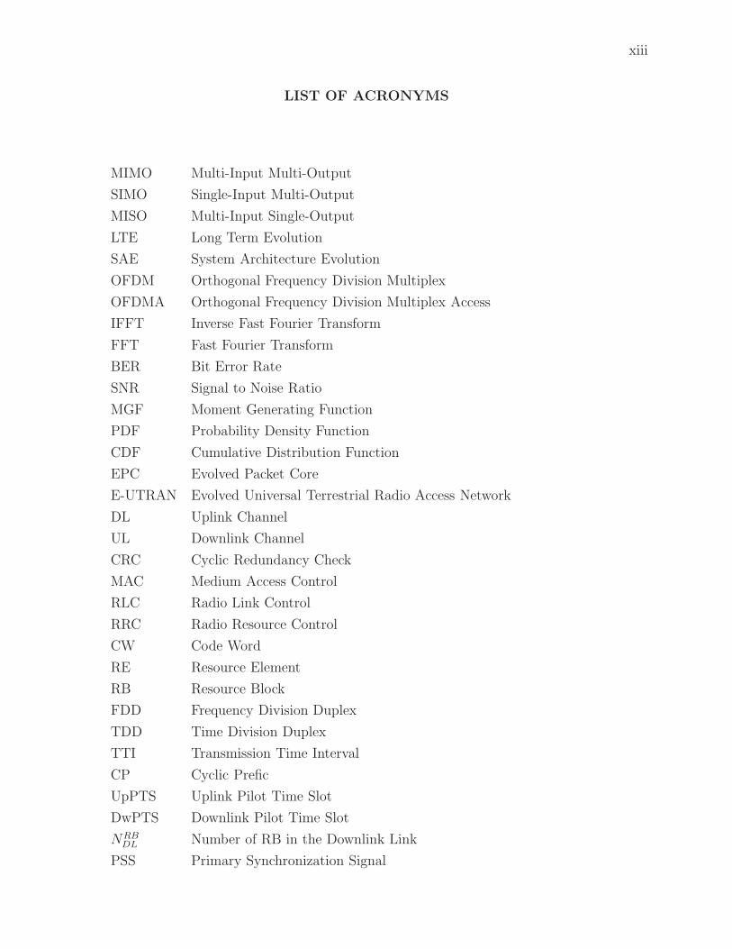
LIST OF ACRONYMS

MIMO Multi-Input Multi-Output

SIMO Single-Input Multi-Output

MISO Multi-Input Single-Output

LTE Long Term Evolution

SAE System Architecture Evolution

OFDM Orthogonal Frequency Division Multiplex

OFDMA Orthogonal Frequency Division Multiplex Access

IFFT Inverse Fast Fourier Transform

FFT Fast Fourier Transform

BER Bit Error Rate

SNR Signal to Noise Ratio

MGF Moment Generating Function

PDF Probability Density Function

CDF Cumulative Distribution Function

EPC Evolved Packet Core

E-UTRAN Evolved Universal Terrestrial Radio Access Network

DL Uplink Channel

UL Downlink Channel

CRC Cyclic Redundancy Check

MAC Medium Access Control

RLC Radio Link Control

RRC Radio Resource Control

CW Code Word

RE Resource Element

RB Resource Block

FDD Frequency Division Duplex

TDD Time Division Duplex

TTI Transmission Time Interval

CP Cyclic Prefic

UpPTS Uplink Pilot Time Slot

DwPTS Downlink Pilot Time Slot

NRBDL Number of RB in the Downlink Link

PSS Primary Synchronization Signal

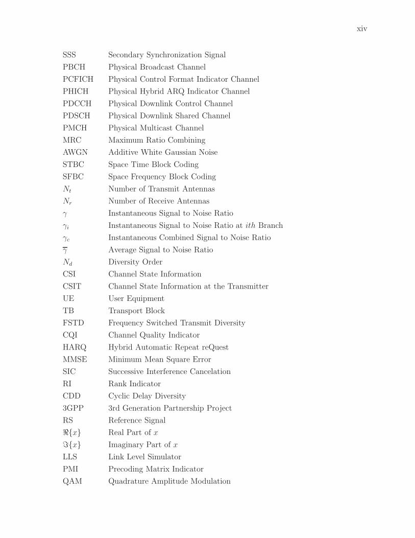
xiv

SSS Secondary Synchronization Signal

PBCH Physical Broadcast Channel

PCFICH Physical Control Format Indicator Channel

PHICH Physical Hybrid ARQ Indicator Channel

PDCCH Physical Downlink Control Channel

PDSCH Physical Downlink Shared Channel

PMCH Physical Multicast Channel

MRC Maximum Ratio Combining

AWGN Additive White Gaussian Noise

STBC Space Time Block Coding

SFBC Space Frequency Block Coding

Nt Number of Transmit Antennas

Nr Number of Receive Antennas

γ Instantaneous Signal to Noise Ratio

γi Instantaneous Signal to Noise Ratio at ith Branch

γc Instantaneous Combined Signal to Noise Ratio

γ Average Signal to Noise Ratio

Nd Diversity Order

CSI Channel State Information

CSIT Channel State Information at the Transmitter

UE User Equipment

TB Transport Block

FSTD Frequency Switched Transmit Diversity

CQI Channel Quality Indicator

HARQ Hybrid Automatic Repeat reQuest

MMSE Minimum Mean Square Error

SIC Successive Interference Cancelation

RI Rank Indicator

CDD Cyclic Delay Diversity

3GPP 3rd Generation Partnership Project

RS Reference Signal

ℜ{x} Real Part of x

ℑ{x} Imaginary Part of x

LLS Link Level Simulator

PMI Precoding Matrix Indicator

QAM Quadrature Amplitude Modulation

1

CHAPTER 1

INTRODUCTION

1.1 Introduction

To increase the capacity and speed of wireless communication systems, a new type of

wireless data networks has recently emerged and been standardized by the 3rd Generation

Partnership Project (3GPP). This new standard comes as a natural evolution to the existing

second (2G) and third (3G) generation wireless networks in order to respond to the growing

demand in terms of extended data rates and speed and is marketed as the 4G Long Term

Evolution (LTE) network. It was first proposed by NTT DoCoMo of Japan in 2004, and

studies on the new standard officially commenced in 2005. In may 2007, the LTE and

the System Architecture Evolution (SAE) Trial Initiative (LSTI) was founded as a global

collaboration between vendors and operators with the goal of verifying and promoting the

new standard in order to ensure as quickly as possible the global introduction of the new

technology. The LTE standard was finalized in December 2008, and the first publicly available

LTE service was launched by TeliaSonera in Oslo and Stockholm on December 2009 as a

data connection with a Universal Serial Bus (USB) modem. By the end of 2012 already 113

commercial LTE networks in 51 countries have been deployed and the Global mobile Suppliers

Association (GSA) forecasts, by the end of 2013, that the number of deployed commercial

LTE networks will reach 209 in 75 countries. In Canada, Rogers Wireless was the first wireless

network operator to launch LTE network on July, 2011 offering the Sierra Wireless AirCard

USB mobile broadband modem known as the LTE Rocket stick. Initially, CDMA operators

planned to upgrade to rival standards called Ultra Mobile Broadband (UMB) and WiMAX,

but finally all the major CDMA operators in the world have announced that they intended to

migrate to LTE after all. The most recent evolution of LTE has been standardized in March

2011 and is known as LTE-Advanced. The LTE-Advanced services are expected to begin in

2013. Comparing with other standards, the key aim of UMTS and GPRS/EDGE was the

expansion of service provision beyond voice calls towards a multi service air interface. This

objective was achieved by circuit switching and packet switching. In contrast to the former

technology family of standards, LTE was designed from the start with the goal of evolving the

the radio access technology under the assumption that all services would be packet switched,

rather than following the circuit switching model of earlier systems.

2

1.2 Motivation

The third generation (3G) wireless communication systems, mainly based on the WCDMA

technology, have been confronted with a number of new challenges regarding to the design

of the required wireless communication systems. The main challenges the 3G technology has

been facing can be summarized as follows:

– The data rate of the 3G system needs to be increased by introducing new techniques

such as HSPA and HSPA+. Since the 3G is based on WCDMA technology in a 5 MHz

bandwidth, the data rate couldn’t be improved as much as planned.

– The typical delay spread observed in wireless channel puts a strong limitation on the

symbol duration period if it is transmitted serially. To struggle with the time delay

spread of the wireless channel, the delay spread should be smaller than the symbol

period, which is not the case for high data rate serial transmission, where, in general,

the delay spread is much bigger than the transmitted symbol period. It is well known

that the delay spread of the channel causes Inter Symbol Interference (ISI) which can be

undone often only partially by means of complex equalization procedures. In WCDMA,

since the signal is transmitted serially in time it is highly challenging to increase the

data rate of the transmitted signal.

To contend with the above mentioned challenges and to achieve good system performance,

the choice of an appropriate modulation and multiple access schemes applicable to mobile

wireless communication systems is then critical. In this context, the parallel multi carriers

schemes have shown their efficiency in many wireless applications. More specifically, the Or-

thogonal Frequency Division Multiplexing (OFDM) which is a special case of multi carrier

transmission is a good choice. In OFDM, the frequency selective fading wide band channel

is used as frequency multiplex of non frequency selective (flat fading) narrow band paral-

lel sub channels. To avoid the need to separate the carriers by means of guard-bands and

therefore make OFDM highly spectrally efficient, the sub channels in OFDM are overlapping

and orthogonal. Initially, only analog design was considered, using banks of sinusoidal signal

generators and demodulators to process the signal for multiple sub channels. The tremen-

dous advancement in digital signal processing made the implementation of digitally designed

OFDM possible and cost effective using the Discrete Fast Fourier Transform (DFFT). The

OFDM became the modulation of choice for many applications for both wired systems (such

us Asymmetric Digital Subscriber Line (ADSL)) and wireless broadcasting systems such as

Digital Audio Broadcasting (DAB) and Digital Video Broadcasting (DVB) as well as Wireless

3

Local Area Network (WLAN). In addition to the mentioned benefits of OFDM technology,

this multi carrier modulation has the ability to be adapted in a straightforward manner to

operate in different channel bandwidth according to spectrum availability. All above men-

tioned benefits have strongly motivated the choice of OFDM in the LTE system. Beside the

OFDM schemes, the use of multi antenna techniques always been known to be of value in

improving the performance of general wireless communication systems including early line

of sight systems. Nevertheless, most of the theoretical development in understanding their

fundamental benefits has appeared only in the last 15 years, driven by advancement in signal

processing and Shannon’s information theory. A key innovation being accomplished with the

introduction of the concept of so-called Multiple Input Multiple Output (MIMO) systems in

the mid-1990s. In fact, serious attention to the utilization of multiple antenna techniques in

mass market commercial wireless networks has only been granted since around 2000. The

key role that MIMO technology plays in the latest wireless communication standards for

personal area networks testifies to its importance. The MIMO technique was adopted for the

first time in the release 7 version of HSDPA (High Speed Downlink Packet Access) and LTE

is the first wireless communication system to be developed with MIMO as a key component

form the start. In chapter 2, we will provide the necessary theoretical background for a good

understanding of the role and advantage promised by MIMO techniques in general wireless

communication.

1.3 Research Objective and Contributions

Nowadays, the performance evaluation of LTE systems is mainly obtained through rather

time consuming simulators and it is extremely difficult to evaluate the influence of the different

parameters. The objective of this dissertation is to derive analytical models that will partially

compensate for these drawbacks. More specifically, we focus on the link level performance

of the physical layer. Three main key performance indicators are considered in this study,

namely the Bit Error Rate (BER), Channel Capacity as well as the data throughput, all

in terms of Signal to Noise Ratio (SNR). We also consider to analyze and evaluate MIMO

systems using antenna selection techniques. In a first step, we analyze the BER performance

of MIMO system when antenna selection is applied at the receiver side. In a second step, we

evaluate the impact of antenna correlation on the BER performance of MIMO systems using

receive antenna selection. A subject rarely considered in the current literature.

4

1.4 Dissertation Outline

In this work we provide several analytical performance analysis of MIMO schemes defined

in the 4G LTE standard as well as comparison with simulations results which we believe are

significant contributions. The document pertaining to this thesis is organized as follows:

– In Chapter 2, we present a technical overview of LTE systems. More specifically, the

system architecture of LTE is highlighted and explained. Since our study concentrates

on the physical layer of LTE systems, we emphasize particularly the OFDMA and

MIMO schemes used by the LTE systems. The overall frame structure of the LTE

signal is also considered with some depth.

– The main performance analysis of different MIMO scheme scenarios in LTE are given

in Chapter 3. At first, we describe the system model used for the analysis. Then, the

detailed Bit Error Rate analysis with mathematical derivation for different modulation

order and different MIMO arrangements are developed. The approach used for this

analysis is based on the Probability Density Function (PDF) of the instantaneous Signal

to Noise Ratio (SNR) and the Moment Generating Function (MGF) approach. The

channel capacity as well as data throughput are also derived in this chapter. To validate

the accuracy of our analysis, simulation results of the analysed schemes are shown and

compared to the analytical results.

– In Chapter 4, the principles and performance analysis of the Antenna selection algo-

rithm of MIMO Systems are presented. After a brief introduction, the system model

used for our analysis is given. A subsection dedicated to the BER performance analysis

for receive antenna selection follows the introduction. The theory of order statistics

used for this analysis is also introduced in this section. To validate the analytical re-

sults, the simulations results of antenna selection algorithm are shown and compared

to the numerical results. In the second part of this chapter, the impact of antenna

correlation on the performance of MIMO systems using antenna selection is evaluated.

The system model used for this evaluation is also shown in this section.

– The summary and conclusion of this dissertation are made in Chapter 5, where we

outline the basic contributions of the overall work and present an outline of possible

future extensions.

5

CHAPTER 2

TECHNICAL OVERVIEW OF LTE SYSTEMS

In this chapter, a brief technical overview of the LTE systems is provided. We start by

a brief description of the high level overall LTE system architecture, which consists of two

parts; namely the radio and core network parts as shown in Figure 2.1. Since our main

work in this thesis is related to the performance of the LTE physical layer, we will detail,

more specifically, the physical layer of the radio part of LTE system. Due to its significant

importance and relevance in our analysis and evaluation, one section is dedicated to the frame

structure of the physical layer in which we explain how the data is organized in the time and

frequency domains as well as how the data is transmitted over the air. Finally, we conclude

the chapter by presenting the MIMO-OFDM schemes as defined in LTE which are relevant

to our study.

2.1 LTE System Architecture

Figure 2.1 LTE System Architecture.

To understand the general structure of 4G (also called Evolved 3G) wireless commu-

nications systems, it is primordial to know its overall network architecture as well as the

6

functionalities of each element. As any other wireless communications network, the 4G sys-

tem consists of two main parts, namely the core network part and the radio part. The core

side of the network is called System Architecture Evolution (SAE) and the radio part is

known as Long Term Evolution (LTE). The term LTE encompasses the Evolved Universal

Terrestrial Radio Access Network (E-UTRAN) and represents the radio access network. The

description of each part will be presented separately in the following subsections.

2.1.1 Core Network

At the beginning of the standardization process, the core network of the Evolved 3G

network was designated by SAE but nowadays the core network is also called Evolved Packet

Core (EPC) and the term SAE is used in parallel with EPC. The main functionality of the

EPC is to provide access to external packet networks based on Internet Protocol (IP) and

performs a number of functions for idle and active terminals. The whole functionalities of

the core network (EPC) are performed using the following main logical nodes:

– Packet Data Network (PDN) Gateway (P-GW)

– Serving Gateway (S-GW)

– Mobility Management Entity (MME)

The main functionality of P-GW is to allocate IP addresses for the user equipment (UE).

It is responsible for the filtering of downlink user’s IP packets into the different radio ser-

vices. Serving Gateway acts as the local mobility anchor for the data transmission when user

equipment moves between eNodeBs. A mobile anchor means that the data for a specific user

equipment pass through the S-GW regardless of the serving eNodeB to which the mobile

is connected. The main functionality of the Mobility Management Entity is to process the

signaling between the user equipment and the core network.

2.1.2 The Access Network

The access network of LTE, i.e., E-UTRAN, consists of a network of base stations called

eNodeBs, as illustrated in Figure 2.1 above. In this Figure, a user equipment (UE) is con-

nected to eNodeB#2 using the radio interface. The elements of the core network; namely the

MME and S-GW as described in the previous section are also shown in this Figure. The eN-

odeBs are connected to the core network (EPC) via S1 interfaces. Two types of S1 interfaces

are standardized in LTE. The S1-U, referred to as S1 User plan interface and S1-C, referred

to as S1 Control plan interface. The communications between eNodeBs is also possible in

LTE and it is assured by the so called X2 interfaces which enable a meshed radio access

7

network (RAN) architecture. The E-UTRAN is responsible of all functions related to the

radio interface and its main function can be summarized briefly as follows:

– Connectivity to the EPC : This function handles the radio communications between the

mobile user and the EPC network.

– Radio Resource Management (RRM)- This covers all functions related to the radio

bearers such as radio bearer control, radio admission control, radio mobility control,

scheduling and dynamic allocation of resources to UE in both uplink and downlink.

Radio bearer can be defined as a pipeline connecting two or more points in the com-

munication system in which data traffic follow through.

– Header compression: This function helps to provide efficient use of the radio interface

by compressing the IP packet headers that could otherwise cause a significant overhead,

especially for small packets such as voice over IP.

– Security : All data sent over the radio interface is encrypted.

In LTE, the radio interface, also called Uu interface, protocols that run between eNodeBs

and an UE are divided into two plans, namely the user plan and the control plan. The

control plan protocols are responsible for managing the control signaling whereas the user

plan is responsible for transporting user traffic data. In Figure 2.2, the protocol stacks of the

user plan are shown, where PDCP (Packet Data Convergence Protocol), RLC (Radio Link

Control), MAC (Medium Access Control) and PHY (Physical) sublayers perform functions,

such as header compression, retransmissions during handover, segmentation and reassembly

of upper layers packets, scheduling and multiplexing data from different control channels. To

be complete, the protocol stacks of the interface between the eNodeB and the serving GW,

called S1-U interface, is also shown in Figure 2.2.

The protocols stacks of the control plan appear in Figure 2.3. It can be seen from the

figure that the control plan protocols differ only by the so-called Radio Resource Control

(RRC) sublayer with respect to the user plan protocols. In fact, all other sublayers perform

the same functions as in the user plan. For the control plan, the eNodeB interfaces with the

MME entity and the interface between them are designated by S1-MME as shown in Figure

2.3.

The above is just an outline of the actual architecture of the LTE concept. Since our

main work in this thesis is related to the LTE physical layer aspects, more details about the

LTE physical layer will be presented in the forthcoming sections.

8

Figure 2.2 User Plan Protocols.

Figure 2.3 Control Plan Protocols.

2.2 LTE Physical Layer

The role of the physical layer in LTE is mainly to transform the base-band data into a

reliable signal for transmissions across the radio interface between the eNodeB and the User

Equipment (UE) in both directions, i.e., from eNodeB to UE, (Downlink Channel (DL)),

and from UE to eNodeB, (Uplink Channel (UL)). The simplified block diagram of the LTE

downlink physical layer is shown in Figure 2.4.

Each block of data, received from the upper layer (MAC layer) (See Figures 2.2 and 2.3)

is first protected against transmission errors, usually first with Cyclic Redundancy Check

(CRC). Then using Turbo codes, the block of data is coded to form a codeword (CW). After

9

Figure 2.4 LTE downlink Physical Layer Block Diagram.

channel coding, an initial step of scrambling is applied to the physical channel, and serves

the purpose of interference rejection. The scrambling task is performed using an order 31

Gold code, that can provide 231 sequences with no cyclic shifts. The attractive feature of

Gold codes is that they can be generated with very low implementation complexity, as they

can be derived from the modulo-2 addition of two maximum length sequences, which can

be generated by a simple shift register. Following the scrambling operation, the transmitted

data bits are mapped into modulated complex value symbols depending on the modulation

scheme which is used. After modulation task, a layer mapping is applied to the modulated

codewords (CW). In LTE, a layer mapper maps the modulated symbols belonging to either

1 or 2 codewords into a number of layers less or equal to the number of antennas ports. In

LTE, antenna port is a new term used to differentiate with the physical antenna. Usually,

antenna ports map into physical antenna elements. A more formal definition of antenna port

will be given later in this chapter. An operation of precoding follows the layer mapping,

which consists of applying coding to the layers of modulated symbols prior to mapping onto

Resource Element (RE). The concept of Resource Element will be explained later in section

2.3. The final stage of the LTE block diagram is the transformation of the complex modulated

symbols at the output of RE mapper into a complex valued OFDM signal by means of an

Inverse Fast Fourier Transform (IFFT).

As indicated in Figure 2.4, the LTE downlink transmission is based on Orthogonal Fre-

quency Division Multiplexing Access (OFDMA). OFDMA is known as a technique of encod-

ing digital data on multiple carrier frequencies. The principle of OFDMA is to convert a

wide band frequency-selective channel into a set of many flat-fading subchannels using op-

timum receivers that can be implemented with a reasonable system complexity, in contrast

10

to WCDMA systems. Another important advantage of OFDMA is the easy frequency do-

main scheduling, typically by assigning only good channels (i.e., channels with high SNRs)

to the users. It is well known that OFDMA is an efficient technique to improve the spectral

efficiency of wireless systems [38]. By converting the wide-band frequency-selective channel

into a set of several flat fading sub-channels, OFDM becomes more resistant to frequency

selective fading than single carrier systems. Since OFDM signals are in time and frequency

domains, in addition to the use of time domain scheduling, a frequency domain scheduling

can also be used. The role of the user scheduler at the transmitter side is to assign the data

rate for each user according to the channel conditions from the serving cell, the interference

level from other cells, and the noise level at the receiver side. It has been proven [43] that in

LTE, for a given transmission power, the system data throughput and the coverage area can

be optimized by employing Adaptive Modulation and Coding (AMC) techniques.

2.3 LTE Frame Structure

Two types of LTE frame structures are defined depending on the duplexing mode of the

transmission. Two duplexing methods are defined in LTE, namely Time Division Duplex

(TDD) and Frequency Division Duplex (FDD). In the FDD mode, the downlink path (DL),

from the eNodeB to UE, and the uplink path (UL), from the UE to eNodeB, operate on dif-

ferent carrier frequencies. In the TDD mode, the downlink and the uplink paths operate on

the same carrier frequency but in different time slots. In other word, in FDD, the downlink

and uplink transmissions are separated in the frequency domain, whereas in TDD the down-

link and uplink transmissions are separated in the time domain. The Type 1 frame structure

of LTE is associated with the FDD duplexing mode whereas the Type 2 frame structure of

LTE is associated with the TDD duplexing mode. For both types of LTE frame structure,

the DL and UL transmissions in LTE systems are arranged into radio frames. The duration

of a radio frame is fixed at 10 ms. The radio frame is comprised of ten 1ms subframes, which

represent the shortest Transmission Time Interval (TTI). Each subframe consists of two slots

of duration 0.5 ms. The Type 1 LTE FDD frame structure is shown in Figure 2.5. In case

of Type 2 TDD frame structure, as shown in Figure 2.6, each radio frame consists of 2 half

frames of 5 subframes each. Subframes can be either uplink subframes, downlink subframes

or special subframes. Special subframes include the following fields: Downlink Pilot Time

Slot (DwPTS) and Uplink Pilot Time Slot (UpPTS).

Depending on the length of the Cyclic Prefix (CP) and the subcarriers spacing, each time

slot consists of 6 or 7 OFDM symbols. In fact, the cyclic prefix represents a guard period

at the beginning of each OFDM symbol which provides protection against multi-path delay

11

Figure 2.5 Type 1 LTE FDD Frame Structure.

Figure 2.6 Type 2 LTE TDD Frame Structure.

spread. To effectively combat the delay spread of the channel, the duration of the cyclic

prefix should be greater than the duration of the multi-path delay spread. At the same time,

cyclic prefix also represents an overhead which should be minimized. Two types of CP were

specified in LTE, namely the normal CP and the extended CP. The structure of the symbols

in a 0.5 ms slot with normal cyclic prefix is shown in Figure 2.7. In normal CP, each slot

12

Figure 2.7 Structure of the symbols in one slot with Normal Cyclic Prefix.

consists of 7 OFDM symbols, however, with extended CP (see Figure 2.7) only 6 OFDM

symbols constitute one slot as shown in Figure 2.8. The duration of the first cyclic prefix

and the subsequent prefixes in terms of sampling time (Ts) are also shown in Figure 2.8. Ts

represents the basic time unit and is given by Ts = 1/(15000 × 2048) seconds. It can be

noticed that the duration of the first cyclic prefix is larger than the subsequent cyclic prefixes.

For the normal cyclic prefix the duration of the first cyclic prefix is defined as (160 × Ts),

whereas the subsequent cyclic prefixes the duration is only (144 × Ts). For extended cyclic

prefix, all prefixes have the same length which is equal to 512×Ts. The normal cyclic prefix

length is proposed to be sufficient for the majority of radio environment scenarios, while the

extended cyclic prefix is intended for radio environment with particularly high delay spreads.

The cyclic prefix is generated by copying the end of the main body of the OFDM symbol.

Now, we explain how OFDM signal is generated. An OFDM symbol is based on the Inverse

Fast Fourier Transform (IFFT), which is an operation of a transformation from frequency

domain to time domain. Accordingly, the transmitted signal (the input signal to the OFDM

block in Figure 2.4) is defined in the frequency domain. This means that the complex modu-

lated symbols are considered as the coefficients in the frequency domain. The block diagram of

an OFDM system is shown in Figure 2.9. The serial input data symbols (modulated synbbols)

are firstly converted into a block of parallel complex S[k] = [S0[k], S1[k], S2[k], ..., SM−1[k]]T

of dimension, where k is the index of an OFDM symbol containing M subcarriers. The M

parallel data streams are first independently modulated (e.g. QPSK or M-QAM modulation)

to form a vector of complex modulated symbols X[k] = [X0[k], X1[k], X2[k], ..., XM−1[k]]T .

13

Figure 2.8 Structure of the symbols in one slot with Extended Cyclic Prefix.

The X[k] vector is then applied to the input of an N -point Inverse Fast Fourier Trans-

form (IFFT). The output of this operation is a set of N complex time-domain samples

x[k] = [xo[k], x1[k], x2[k], ..., xN−1[k]]T . It is worth noting that in practical implementation

of an OFDM system, the number of the points used by IFFT (N ) is greater than the number

of the modulated subcarriers (M ) (i.e., N ≥ M). As shown in Figure 2.9, the un-modulated

subcarriers are being padded with zeros. The next important operation in the geenration

of an OFDM signal is the creation of a guard period at the beginning of each OFDM sym-

bol x[k] by adding a Cyclic Prefix (CP). This CP is simply generated by taking the last G

samples of the IFFT output and appending them at the beginning of x[k]. This yields the

OFDM symbol in time domain as: [xN−G[k], ..., xN−1[k], x0[k], x1[k], x2[k], ..., xN−1[k]] as

shown in Figure 2.9. The last step in the OFDM signal generation is the parallel to serial

conversion of the IFFT output for transmissions through the radio interface.

The results of the OFDM operation in LTE is that the output signal now possesses two

domains; the frequency domain and the time domain. The frequency domain is represented

by successive subcarriers and the time domain is represented by successive OFDM symbols.

In LTE, the bandwidth of a subcarrier is defined to be 15 KHz or 7.5 KHz. In the frequency

domain, resources are grouped in units of 12 subcarriers. Thus, for a subcarrier spacing of

15 KHz, 12 subcarriers occupy a total of 180 KHz. The combination of 12 subcarriers in one

slot (7 OFDM symbol) form what is called Resource Block (RB). The smallest of resource is

called Resource Element (RE), which consists of one subcarrier for a duration of one OFDM

Symbol. The structure of Resource Block for 15 KHz subcarrier spacing and its constituting

14

Figure 2.9 OFDM Signal Generation.

REs are shown in Figure 2.10 for illustration.

The number of RB in the frequency domain (NRBDL in Figure 2.10) depends on the trans-

mission bandwidth. LTE is designed as a scalable system where the channel bandwidth is

flexible. In fact, the standard defines six channel bandwidths. The possible channel band-

width as defined in LTE for 15 KHz subcarriers spacing is shown in Table 2.1. The number

of IFFT size is also shown in Table 2.1. For example in a 5 MHz bandwitdh, the IFFT size

is set to 512 but the number of the used subcarriers is only 300, which represent 25 RB of 12

subcarriers each.

So far, we showed how the signal is generated to be sent over the radio interface. But how

the data is organized and what kind of information are transmitted? In LTE, the physical

layer receives different data types from the higher layer (MAC layer) which are organized in

the form of different channels, called Transport Channels. The MAC layer itself receives data

from the RLC layer in the form of Logical channels. Before sending the transport channels

15

Figure 2.10 LTE Resource Block.

Table 2.1 Resource Block as a function of Channel Bandwidth

Channel Bandwidth 1.4 MHz 3 MHz 5 MHz 10 MHz 15 MHz 20 MHzResource Blocks in the frequency domain 6 15 25 50 75 100FFT Size (N ) 128 256 512 1024 1536 2048Subcarriers in the frequency domain (M ) 72 180 300 600 900 1200Total Subcarriers badwidth (MHz) 1.095 2.715 4.515 9.015 13.515 18.015

into the air, the physical layer process the transport channels to form Physical Channels. In

addition to the physical channels, the physical layer needs to create its own signals to be

sent over the air. The signal generated in the physical layer are called Physical Signals. The

principle of channels generation and their placement with respect to different layers in LTE

is illustrated in Figure 2.11.

As indicated in Figure 2.11, we distinguish three types of physical signals and six types

16

Figure 2.11 Physical Channels and Physical Signals in LTE.

of physical channels in LTE and they are defined as follow:

Downlink Physical Signals : Three different physical signals are generated in the physical

layer:

1. Primary Synchronization Signal (PSS)

2. Secondary Synchronization Signal (SSS)

3. Reference Signals (RS)

PSS and SSS are the synchronization signals, used by the UE to achieve radio frame,

subframe, slot and symbol synchronization in the time domain as well as the identification

of the center of the channel bandwidth in the frequency domain. The reference signals (RS)

on the other hand are used for channel estimation purposes and to support channel quality

indicator (CQI) reporting and demodulation. They can also be used to support channel

quality measurements for handover purposes.

Downlink Physical Channels : To carry the information blocks (data) received from the

MAC and higher layers, the number of downlink physical channels are defined in LTE. In

total, six physical downlink channels are defined in LTE as follow:

1. Physical Broadcast Channel (PBCH)

2. Physical Control Format Indicator Channel (PCFICH)

3. Physical Hybrid ARQ Indicator Channel (PHICH)

17

4. Physical Downlink Control Channel (PDCCH)

5. Physical Downlink Shared Channel (PDSCH)

6. Physical Multicast Channel (PMCH)

The PBCH channel is used to broadcast the master information block (MIB) using trans-

port and logical channels from higher layers (MAC and RLC layers). The PBCH is allocated

the central 72 subcarriers belonging to the first 4 OFDM symbols of the second time slot

of every 10 ms radio frame, which corresponds to 240 resource elements (RE) excluding the

resource elements used by the RS ((72×4)−48), where 48 is the number of resource elements

allocated to the Reference Signal. The PCFICH is used at the start of each 1 ms downlink

subframe to signal the number of symbols used for the PDCCH. The PHICH is used to signal

positive or negative acknowledgment for uplink data transferred on the uplink channel. To

transfer the downlink control information, LTE uses the PDCCH channel. The PDSCH is

the main data downlink channel in LTE. It is used for all user data. In addition to the user

data, the system information and paging can also be sent with PDSCH channel. Finally, the

PMCH is used to transfer the multimedia broadcast multicast service application data. More

details about the use of each physical channel is given in [26] and [44]

2.4 MIMO-OFDM Schemes in LTE

Before explaining the MIMO-OFDM schemes as defined in LTE, we provide a brief the-

oretical background of the advantages promised by multiple antenna techniques in wireless

communication systems. In this context, the first part of this section covers the different con-

figurations of using multiple antennas and their corresponding advantages from theoretical

point of view. In the second part, the MIMO schemes as defined in LTE will be explained

and the practical issues that cause the gap between the theoretical predictions and practical

performances of such systems will be discussed.

Traditional wireless communications systems with one antenna at the transmitter and one

antenna at the receiver (Single-Input Single-Output (SISO)) exploit time and/or frequency

domains pre-processing the transmitted signal and decode the received data. Adding addi-

tional antennas either at the transmitter or at the receiver creates an extra spatial dimension

for signal coding and decoding processes. Hence, new areas of processing have emerged such

as Space Time and Space frequency processing. Depending on the availability of additional

antennas at the transmitter and/or at the receiver, such techniques are classified as Single In-

put Multi Output (SIMO), Multi Input Single Output (MISO) or Multi-Input Multi-output

(MIMO). Thus, in the case of having multiple antenna at the base station and only one

antenna at the user’s equipment, the uplink (from user equipment to base station) is referred

18

to SIMO and the downlink (from base station to user equipment) is referred to MISO. It is

worth noting that the term MIMO is sometimes also used in its widest sense, thus including

SIMO and MISO as special cases.

When multiple antennas are available they can be used in different modes. Essentially,

we can distinguish three different modes for multiple antennas, namely beam-forming mode,

diversity mode (receive and transmit) and multiplexing mode. In beam-forming mode the

advantage of using multiple antennas is evaluated by the so called Array gain. For diversity

mode, the diversity gain is usually used to evaluate the advantage of this mode. Finally, the

multiplexing gain is the benefit of using multiplexing mode. The principles of each mode and

their advantages are described and explained in the following subsection:

2.4.1 Array Gain

The first approach of using multiple antennas is to send or to receive the same signals on

all the antennas. In case of multiple receive antennas, a coherent combining techniques can be

realized through spatial processing at the receive antennas side. In case of multiple transmit

antennas, the coherent combining can be realized through spatial processing at the transmit

antennas side. An example of receive coherent combining is the Maximum Ratio Combining

(MRC) method and an example of transmit coherent combining is the concentration of energy

in one or more directions, the so called beam-forming. In both cases, the results of combining

will be reflected in an improvement of average SNR which is represented by an Array gain,

also known as beam-forming gain. The array gain can be defined as the increase of the

average SNR. In case of MRC, it can be shown that the array gain is constant and is equal

to the number of antennas. To illustrate this, we should determine the combined SNR for a

MRC system. To this end, let‘s suppose a MRC system with Nr branches (from one transmit

antenna to Nr receive antennas).

2.4.2 Diversity Gain

For improving the communication reliability and reducing the sensitivity to the fading

channel, we can send or receive the same signal on different antennas. By increasing the

number of independent copies of the transmitted signal, the probabilities that at least one

of the signals is not experiencing a deep fade increase and hence improving the quality and

reliability of reception. This kind of transmissions is known as Diversity Mode and the

associated gain is known as Diversity Gain. In other words, diversity gain corresponds to

the mitigation of the effects of multipath fading, by means of transmitting or receiving over

multiple antennas in which the fading is sufficiently de-correlated. The Diversity Gain can

19

be described either in terms of order, which represents the number of effective independently

diversity branches or in terms of the slope of the Bit Error Rate curve as a function of the

signal to noise ratio at high SNRs.

2.4.3 Multiplexing Gain

Multiple antennas can be used to send different signals on different antennas. The original

high data rate signal is first divided into two low data rate signals and each signal is sent

from different antennas. In the receiver side, the different signals are processed separately

and multiplexed to recover the original high data rate signal. This method is known as

Multiplexing mode and the associated gain is the Spatial Multiplexing gain. To evaluate

this multiplexing gain, we use to the basics of shannon theory of capacity and spectral

efficiency calculations. To this end, in the case of single antenna system (SISO), the data rate

calculation is related to the Shannon capacity formula which yields the maximum achievable

data rate of a single communication link in Additive White Gaussian Noise (AWGN) channel

as [7]:

C = B log2(1 + γ) (2.1)

where C is the capacity, or maximum error free data rate; B is the bandwidth of the channel;

and γ is the channel SNR. Since antennas diversity can increase the SNR linearly, diversity

techniques can increase the capacity but in a logarithmic way with respect to the number of

antennas. In other words, as the number of antennas increases, the data rate improvement

rapidly diminishes. However, it can be concluded from the above equation that when the

SNR is low, the capacity can increase linearly with SNR, since log(1 + x) ≈ x for small

x [7]. The goal of multiplexing mode is to get more substantial data rate increase at high

SNRs and to achieve this goal, the multiple antennas are used to send multiple independent

signals. Therefore, the multiplexing mode has the ability to achieve a linear increase in

the data rate with the number of antennas at moderate to high SNRs through the use of

sophisticated signal processing algorithms. Specifically, it is shown that the capacity can

be increased as a multiple of min(Nt, Nr) [7]. The capacity improvement is limited by the

minimum of the number of antennas at either the transmitter or the receiver. As an example,

a single user MIMO communications between a base station with four antennas and a user

equipment with two antennas can support multiplexing of two data signals (also called data

stream), and therefore doubling the data rate of the user equipment compared with a single

antenna case. To achieve this maximum multiplexing gain, the different subchannels should

experience different and de-correlated responses. In ideal case, in high SNR regions and in

20

rich scattering environments, the multiplexing gain will be equal to two. However in a real

environment, a lower value of multiplexing gain can be observed.

Before describing the multiple antenna schemes in LTE, some terminology should be

explained. Especially, four main terminologies have been introduced and are widely used in

LTE, namely the Antenna ports ; spatial layer ; the rank and the codeword .

– Antenna ports : In LTE, the concept of antenna ports is used and should not be confused

with the physical antenna elements. In fact, antenna ports are mapped into physical

antenna elements. A downlink antenna port is defined by its associated Reference

Signal. For example, antenna port 0 is associated with a cell specific Reference Signal,

whereas antenna port 6 is associated with a positioning Reference Signal. The complete

set of downlink antenna ports and their associated Reference Signals can be found in

the Table 2.2:

Table 2.2 Antenna ports and their associated Reference Signals

Antenna Port 3GPP Release Reference Signal0 to 3 8 Cell Specific Reference Signal

4 8 MBSFN Reference Signal5 8 UE Specific Reference Signal6 9 Positioning Reference Signal

7 to 8 9 UE Specific Reference Signals9 to 14 10 UE Specific Reference Signals15 to 22 10 CSI Reference Signals

– Spatial Layer : In LTE, this term is used for one of different streams generated by

spatial multiplexing. A layer can be described as a mapping of symbols into the transmit

antenna ports. This operation is known as layer mapping where the modulated symbols

are mapped into a number of layers where the number of layers are equal to the number

of antenna ports.

– The Rank of the transmission is equal to the number of transmitted layers

– A CodeWord (CW) corresponds to a single Transport Block (TB) and it is an inde-

pendently encoded data block delivered from the Medium Access (MAC) layer, and

protected by a CRC.

Note that the number of codewords is always less than or equal to the number of layers,

which in turn is always less than or equal to the number of antenna ports. For a rank greater

than one, two codewords can be transmitted.

Based on the above mentioned theoretical background and terminologies, the MIMO

schemes adopted for LTE Release 8 and 9 can be reviewed and explained. These schemes

21

relate to the downlink unless otherwise stated.

2.4.4 Diversity Schemes in LTE

In LTE, two main transmit diversity schemes are employed; the first one with 2 transmit

antennas and the second one with 4 transmit antennas. Both schemes use only one data

stream (one signal). In LTE, one data signal (also called data stream) is referred as one

codeword because only one transport block (TB) is used per data stream. The transport

block itself is defined as the unit of transmitted data and it corresponds to the Medium

Access Control (MAC) layer Protocol Data Unit (PDU). The Transport Block unit can be

passed from the MAC layer to the physical layer once per Transmission Time Interval (TTI),

where a TTI is fixed to 1 ms, corresponding to the duration of one subframe as described in

the LTE frame structure section. In order to ensure uncorrelated channels between different

antennas and hence maximizing the diversity gain, the antennas should be well separated

relative to the wavelength. The use of different antenna polarization is another approach

that has demonstrate its efficiency in order to guarantee uncorrelated antennas. If a physical

channel in LTE is configured for transmit diversity operation using two eNodeB antennas, the

diversity scheme is called Space Frequency Block Codes (SFBC). The principle of operation

of SFBC transmission is shown in Figure 2.12. As can be seen from Figure 2.12, the SFBC

Figure 2.12 Space Frequency Block Coding (SFBC) Scheme in LTE

22

diversity scheme is, in fact, exactly the frequency domain of the well known Space Time Block

Codes (STBC), developed by Alamouti [5]. The fundamental characteristic of this family of

code is that the transmitted diversity streams are orthogonal and they can be simply decoded

using a linear receiver. It is worth noting that the STBC is already used in UMTS and it

operates on pairs of adjacent symbols in the time domain. In LTE, however, the number of

available OFDM symbols in a subframe is often an odd number, and hence the application

of STBC is therefore not straight forward for LTE. Instead of adjacent symbols in the time

domain, in LTE the diversity scheme operates on pairs of adjacent subcarriers, leading to a

SFBC.

For SFBC transmission, the transmitted symbols from two eNodeB antenna ports on each

pair of adjacent subcarriers are defined as follow [44]:

[y(0)(1) y(0)(2)

y(1)(1) y(1)(2)

]=

[x1 x2

−x∗2 x∗

1

](2.2)

where y(p)(k) denotes the symbols transmitted on the kth subcarrier from antenna port p.

Figure 2.13 Frequency Switched Transmit Diversity (FSTD) Scheme in LTE

23

In matrix form, the transmitted space frequency block matrix can be generated as follows:

y(0)(1)

y(0)(2)

y(1)(1)

y(1)(2)

=

1√2

1 0 i 0

0 1 0 i

0 −1 0 i

1 0 −i 0

ℜ{x1}ℜ{x2}ℑ{x1}ℑ{x2}

(2.3)

In case of four transmit antennas (antennas port 0 to 3) and in order to keep the or-

thogonality of the code, the diversity scheme is simply a combination of SFBC scheme and

Frequency Switched Transmit Diversity (FSTD) [44]. FSTD implies that a pair of modulated

symbols are transmitted using SFBC scheme with two antennas whereas the other two anten-

nas are not transmitting. In other words, in FSTD, the transmission is alternated between

a pair of transmit antennas. This means that the first two symbols are transmitted on the

antennas 0 and antenna 2, whereas nothing is transmitted on antennas ports 1 and 3. For the

next two symbols, the antennas port 1 and 3 are used for transmission whereas antenna port

0 and 2 are not transmitting. The principle of FSTD diversity scheme is shown in Figure

2.13.The transmission matrix of the FSTD scheme can be then described as follow:

y(0)(1) y(0)(2) y(0)(3) y(0)(4)

y(1)(1) y(1)(2) y(1)(3) y(1)(4)

y(2)(1) y(2)(2) y(2)(3) y(2)(4)

y(3)(1) y(3)(2) y(3)(3) y(3)(4)

=

x1 x2 0 0

0 0 x3 x4

−x∗2 x∗

1 0 0

0 0 −x∗4 x∗

3

(2.4)

where, as previously, y(p)(k) denotes the symbols transmitted on the kth subcarrier from

antenna port p. This space frequency code is known as Frequency Switched Transmit Diver-

sity (FSTD). It can be noticed form the code matrix that on each subcarrier slot, only two

antennas are transmitting. For the first subcarrier slot, the antennas ports 1 and 2 are not

transmitting any signals. We will show in the performance analysis in Chapter 3 that this

scheme is equivalent to the 2× 2 scheme.

2.4.5 Spatial Multiplexing Schemes in LTE

In LTE, a spatial multiplexing mode can either use a single codeword mapped to all

the available layers, or two codewords each mapped to one or more different layers. The

main advantage of using only one codeword is a decrease in the amount of control signaling

required, both for Channel Quality Indicator (CQI) reporting and for HARQ ACK/NACK

feedback. In fact, in case of one single codeword, a single value of CQI is needed for all layers

24

and only one ACK/NACK would have to be signaled per subframe per user equipment (UE).

In the case of using two codewords, more control signaling will be required but the advantage

of such mapping is that significant multiplexing gain can be possible by using Minimum Mean

Square Error and Successive Interference Cancelation (MMSE-SIC ) receiver. The codeword

to layer mapping are shown in the Table 2.3 [44]:

Table 2.3 Codewords-to-layer Mapping in LTE

Transmission Rank Codeword 1 Codeword 2Rank 1 Layer 1Rank 2 Layer 1 Layer 2Rank 3 Layer 1 Layer 2 and Layer 3Rank 4 Layer 1 and layer 2 Layer 3 and layer 4

Depending on the availability of feed back from the user equipment, two modes of spatial

multiplexing were defined in LTE, namely the open loop spatial multiplexing and the closed

loop spatial multiplexing modes. The open loop spatial multiplexing mode was introduced in

release 8 version of the 3GPP specification and it has not changed within the release 9 and

10 versions of specification. In open loop approach, the UE provides feedback to eNodeB in

terms of Rank Indicator (RI) and Channel Quality Indicator (CQI). The RI feedback provides

information about the suggested number of layers whereas the CQI provides information

about the transport block size. In addition to the RI and CQI feedback, the closed loop

spatial multiplexing provides an additional feedback in terms of Precoding Matrix Indicator.

The precoding matrix, selected from a defined codebook, is used to form the transmitted

layers. Each codebook consists of a set of predefined precoding matrices, with the size of the

set being a tradeoff between the number of signaling bits required to indicate a particular

matrix in the code book and the suitability of the resulting transmitted beam direction. The

difference between open loop and closed loop is that in open loop the UE does not provide

any information about the precoding matrix and it is generated independently, whereas in

closed loop the precoding matrix is suggested by the UE. In case of two antenna ports, the

2× 2 spatial multiplexing always transfers 2 codewords using 2 layers during each subframe

see Table 2.4 [26].

For the case of 4 antennas ports, one or two codewords can be transferred during each

subframe. Table 2.5 summarizes the number of codewords and layers which are supported

by a 4× 4 open loop spatial multiplexing.

25

Table 2.4 Codewords, layers and antenna ports for 2× 2 open loop spatial multiplexing.

Number of Codewords Number of Layers Number of Antenna Ports2 2 2

Table 2.5 Codewords, layers and antenna ports for 4x4 open loop spatial multiplexing.

Number of Codewords Number of Layers Number of antennas ports1 2

42

2 34

In open loop spatial multiplexing, instead of sending only two different signals, an ad-

ditional precoding operation is applied to the transmitted signals before being transmitted

onto the radio interface. The precoding scheme adopted for LTE is the so-called Large Delay

Cyclic Delay Diversity (CDD). It should be noted that CDD is not used in LTE as an exact

diversity scheme, as its name stipulate, but rather as a precoding scheme for spatial multi-

plexing mode and that is why it was not introduced in the diversity schemes section. This

CDD precoding is defined using the following equation [26]:

y(0)(i)

.

.

.

y(P−1)(i)

= W (i)×D(i)× U ×

x(0)(i)

.

.

.

x(v−1)(i)

(2.5)

where P is the number of output antenna ports, i is the sample number and v is the

number of input layers. It is worth noting that the precoding multiplication is a function of

the sample number ’i ’ but only the elements within the matrix U are not a function of the

sample number ’i ’. To illustrate the principle of coding, let’s have a closed look to the case

of two transmit antennas and two receive antennas as shown in Figure 2.14. For 2× 2 open

loop spatial multiplexing, 3GPP specifies the W (i); D(i) and U matrix as [26]:

26

W (i) =1√2

[1 0

0 1

](2.6)

D(i) =

[1 0

0 e−j(π)i

](2.7)

U =1√2

[1 0

1 e−j(π)

](2.8)

It can be noticed that the matrix W in case of 2× 2 open loop scheme is fixed and is not

actually a function of ’i ’. The transmitted signal is then obtained by the product of W (i),

D(i) and U as [26]:

W (i)×D(i)× U =1√2

[1 0

0 1

]×[

1 0

0 e−j(π)i

]× 1√

2

[1 0

1 e−j(π)

](2.9)

Figure 2.14 2× 2 Open Loop Spatial Multiplexing with Large-Delay CDD Precoding.

The results of 2.9 depends on the indices ’i ’ of transmitted symbols and hence two different

results are possible, one for odd number and one for even number. For the odd number of

’i ’, is then:

27

W (i)×D(i)× U =1

2

[1 1

1 −1

](2.10)

For even number of ’i ’, the results is found to be:

W (i)×D(i)× U =1

2

[1 1

−1 1

](2.11)

The summary of the described layer mapping and precoding for the 2×2 open loop spatial

multiplexing with two codewords is shown in Figure 2.14:

28

CHAPTER 3

PERFORMANCE EVALUATION OF MIMO SYSTEMS IN LTE

3.1 Introduction

Two main and fundamental key performance indicators which have bee used to evaluate

the performance of the wireless communication systems are the Bit Error Rate (BER)[39],

and the data throughput or its related channel capacity bound. For a system using one an-

tenna at the transmitter and one antenna at the receiver and in non fading AWGN channel,

the evaluation of the BER for most of the known modulation schemes is well known [39].

Using more antennas at the transmitter and at the receiver and also in more realistic fad-

ing channel models, such as Rayleigh, Rician and Nakagami, the evaluation becomes more

complex and necessitates the use and the development of advanced mathematical tools. In

this context, the theory of BER evaluation had experienced an important evolution during

the past decade. Initially, the evaluation of the BER performance was based on a classical

approach where the Gaussian Q-function (also known as Gaussian Probability Integral) was

used (Chapter 4 in [6]). However, this classical approach suffers from two main disadvantages

when extended to more general complex channels especially those experiencing fading. The

first disadvantage is related to the upper infinite limit where it requires a truncation in case

of numerical evaluation. The second and more significant disadvantage is related to the pres-

ence of the argument of the function as the lower limit of the integral. In general case, the

lower limit in the integral depends on other random parameters and this dependency requires

statistical averaging over their probability distribution which poses analytical difficulties. In

other words, to evaluate the average error probability in the presence of fading channels, the

Gaussian Q-function should be averaged over the fading amplitude distribution. To overcome

the mentioned disadvantages, an alternative representation of the Gaussian Q-function has

been developed and since then widely used for the evaluation of the BER (See Appendice

B). In the alternative representation of the Q-function, the argument of the function is nei-

ther the upper nor the lower limit of the integral. Using the alternative representation of

the Gaussian Q-function, the evaluation of the average error probability becomes a problem

of evaluation of the integral of the Laplace transform of the probability density function

of the SNR distribution, which represents the Moment Generation Function (MGF). This

new approach of representation of the Q-function is particularly effective for evaluation of

the average error probability of MIMO schemes where the probability density function of

29

the SNR has more complicated form like the N order Chi-squared distribution. In [29], the

method of MGF was used to evaluate the BER of three phase relaying wireless system using

the Alamouti STBC code [5]. Instead of using the alternative representation of the Gaussian

Q-function, in [30], the Marcum Q-function was used to derive an approximate expression of

BER analysis of Alamouti-MRC scheme with imperfect channel state information in Rician

fading channel. In LTE the BER is mainly evaluated by simulation and to the best of our

knowledge, the BER analysis is rarely treated in the literature. One of our goal is to develop

in this thesis some closed form expressions of the BER for the main MIMO schemes as used

in LTE.

To study the performance of LTE systems, a MATLAB based downlink physical layer

simulator (Appendice C) for Link Level Simulation (LLS) has been developed in [32] [36]. A

System Level Simulation of the Simulator is also available [25]. The main goal in developing

the LTE simulator was to facilitate comparison with the work of different research groups and

it became publicly available for free under academic non-commercial use license [36]. The

main features of the simulator are adaptive coding and modulation, MIMO transmission and

scheduling. As the simulator includes many physical layer features, it can be used for different

applications in research [25]. In [47], the simulator was used to study the channel estimation

of OFDM systems and the performance evaluation of a fast fading channel estimator was

presented. In [42] and [41], a method for calculating the Precoding Matrix Indicator (PMI),

the Rank Indicator (RI), and the Channel Quality Indicator (CQI) were studied and analyzed

with the simulator.

The remainder of this chapter is organized in two main parts. The first part (i.e., section

3.2) is dedicated to the analysis of BER of the major MIMO schemes included in LTE. In

subsection 3.2.1, we set up the system and channel model used in the simulation. In subsection

3.2.2, we present a performance analysis for the average BER of SFBC and FSTD MIMO

schemes. The numerical and simulation results and discussions are presented in subsection

3.2.3. The second part of this chapter (i.e., section 3.3 and section 3.4) considers the capacity

and data throughput evaluation. The capacity analysis is presented in section 3.3.2 followed

by the data throughput evaluation in Section 3.4. The simulations results as well as the

discussions of the obtained results are presented in subsection 3.4.1.

30

3.2 BER Analysis of LTE MIMO Schemes

3.2.1 System Model

In a MIMO system with Nr receive antennas and Nt transmit antennas, the relation

between the received and the transmitted signals on OFDM subcarrier frequency k (k ∈1, ..., N), at sampling instant time n is given by

yk,n = Hk,nxk,n + nk,n (3.1)

where yk,n ∈ CNr×1 is the received output vector, Hk,n ∈ CNr×Ntrepresents the channel

matrix on subcarrier k at instant time n, xk,n ∈ CNt×1 is the transmit symbol vector and

nk,n ∼ CN (0, σ2n.I) is a white, complex valued Gaussian noise vector with variance σ2

n and

I is an Nr × Nr identity matrix. Assuming perfect channel estimation, the channel matrix

and noise variance are considered to be known at the receiver. A linear equalizer filter given

by a matrix Fk,n ∈ CNr×Nris applied on the received symbol vector yk,n to determine the

post-equalization symbol vector rk,n as follows [41]

rk,n = Fk,nyk,n = Fk,nHk,nxk,n + Fk,nnk,n. (3.2)

The Zero Forcing (ZF) or Minimum Mean Square Error (MMSE) design criterion are

typically used for the linear receiver and the input signal vector is normalized to unit power

[53]. In MIMO-OFDM systems, the key factor of link error prediction and performances is

the signal to noise ratio (SNR) which represents the measurement for the channel quality

information. In this study, the SNR is defined as follows [32]:

γk,n =‖Hk,nxk,n‖2F

Ntσ2n

(3.3)

where xk,n is the transmitted symbol vector, ‖.‖2F is the squared Frobenius norm of a matrix.

3.2.2 Average BER Performance analysis for several M-QAM Schemes

In this section, a Bit Error Rate (BER) analysis is presented for Multiple-Input Multiple-

Output (MIMO) schemes in the 3GPP Long Term Evolution (LTE) system. Analytical

expressions for the average BER of the system are derived over flat Rayleigh fading channels

for two different MIMO schemes as defined in LTE, assuming M-ary quadrature amplitude

modulation (M-QAM) schemes and are evaluated numerically. The analysis is based on the

probability density function of the instantaneous Signal to Noise Ratio and the Moment

31

generating function (Appendice C).

Analysis for 2× 1 SFBC-OFDM Scheme

As described in Chapter 2, in LTE, the transmit diversity techniques are defined only for

2 and 4 transmit antennas and one data stream. When two eNodeB antennas are available

for transmit diversity operation, the Space Frequency Block Code (SFBC) is used [43]. SFBC

is based on the well known Space Time Block Code (STBC), derived by Alamouti for two

transmit antennas [5]. STBC is employed with the UMTS and it operates on pairs of adjacent

symbols in the time domain. Since the signal in LTE is a two dimensional signal (in time and

frequency domains) and the number of available OFDM symbols in a subframe is not always

an even number, the direct application of STBC is not straightforward. In LTE, for SFBC

transmission, the symbols are transmitted from two eNodeB antenna ports on each pair of

adjacent subcarriers as follows [43]:

[y(0)(1) y(0)(2)

y(1)(1) y(1)(2)

]=

[x1 x2

−x∗2 x∗

1

](3.4)

where y(p)(k) denotes the symbols transmitted on the kth subcarrier from antenna port p. An

important characteristic of such codes is that the transmitted signal streams are orthogonal

and a simple linear receiver is required for optimal performance.

Since OFDM converts the multipath channel into N frequency-flat fading channel, we

first derive the BER expressions over flat Rayleigh fading channels, given by Pb (E). Then,

the overall average BER over N subcarriers, in each case can be calculated from

BER =1

N

N∑

k=1

Pb,k (E) (3.5)

where the index k (subcarrier index) is ignored for the sake of brevity. In addition, the impact

of cyclic prefix in OFDM is assumed to be negligible.

For the 2× 1 SFBC MIMO scheme, the probability density function of the SNR for each

subcarrier is given by a chi-square distribution function as follows [52]:

f(γ) =2

γ2γe−

2

γγ (3.6)

where γ is the average SNR per symbol given by γ = Es/N0.

To derive the BER, we follow the unified approach to the performance analysis of digital

32

communication systems over generalized fading channel [48]. To this end, we first derive

the expression of Moment Generating Function (MGF) of the derived probability density

function of the instantaneous SNR as [6]:

Mγ(s) =

∫ ∞

0

e−sγf(γ)dγ. (3.7)

Inserting (3.6) into (3.7) and solving the integral, the MGF yields:

Mγ(s) =4

γ2(s+ 2γ)2. (3.8)

The average BER expression for M-QAM modulation scheme can be obtained from [6]

(Equation 8.111; Page 255) as:

Pb (E) ∼= B

√M/2∑

i=1

1

π

∫ π/2

0

Mγ (Ai,θ) dθ (3.9)

where Ai,θ =(2i−1)2

2 sin2 θ3

(M−1)and B is defined by

B = 4

(√M − 1√M

)(1

log2M

). (3.10)

Then, using the MGF expression in (3.8), the associated MGF becomes:

Mγ(Ai,θ) =4

γ2([

(2i−1)2

2 sin2 θ3

(M−1)

]+ 2

γ

)2 . (3.11)

The BER expression is then obtained by substituting (3.11) into (3.9). After some ma-

nipulations, we obtain:

Pb (E) ∼= B

√M/2∑

i=1

1

π

∫ π/2

0

(sin2 θ

sin2 θ + ci

)2

dθ (3.12)

where ci =3(2i−1)2

2(M−1)γ2.

Equation (3.12) represents the average BER performance as a function of γ = Es/N0 and

33

it can be evaluated by numerical evaluation of the integral in (3.12) for M-QAM modulation

schemes. Alternatively, the integral in Equation (3.12) can be solved analytically using [6],

which give us a closed-form expression for the average BER of M-QAM modulation as follows:

Pb (E) ∼= B

√M/2∑

i=1

I2 (π/2, ci) (3.13)

where the closed-form expression for I2(., .) can be obtained from [6] (Eq.5A.24) as follows:

In (φ,D) =1

π

∫ φ

0

(sin2 θ

sin2 θ +D

)n

dθ, −π ≤ φ ≤ π

=φ

π− β

π

{(π2+ tan−1 α

) n−1∑

q=0

(2q

q

)1

(4 (1 +D))q

+ sin(tan−1α

) n−1∑

q=1

q∑

p=1

Tp q

(1 +D)q[cos(tan−1α

)]2(q−p)+1

}(3.14)

where Tp q =

(2q

q

)[(2(q − p)

q − p

)4p [2(q − p) + 1]

]−1

, β =√

D1+D

sgnφ, and α = −β cotφ.

This concludes our analysis of the 2 × 1 SFBC scheme in LTE. In the next section, we

will follow the same approach to derive the BER of the 4× 2 FSTD scheme.

Analysis for the 4× 2 FSTD-OFDM Scheme

In LTE, the frequency space code, designed for 4 transmit antennas is defined as follows:

y(0)(1) y(0)(2) y(0)(3) y(0)(4)

y(1)(1) y(1)(2) y(1)(3) y(1)(4)

y(2)(1) y(2)(2) y(2)(3) y(2)(4)

y(3)(1) y(3)(2) y(3)(3) y(3)(4)

=

x1 x2 0 0

0 0 x3 x4

−x∗2 x∗

1 0 0

0 0 −x∗4 x∗

3

. (3.15)

where y(p)(k) denotes the symbols transmitted on the kth subcarrier from antenna port p.

For the 4× 2 FSTD MIMO scheme, we can show that the instantaneous SNR of the system,

34

for k-th subcarrier, is equivalent to that for a 2 × 2 STBC MIMO system. Therefore, the

probability density function of the SNR is given by a chi-square distribution function as

follows [52]:

f(γ) =8

3γ4γ3e−

2

γγ. (3.16)

In this case, the MGF expression can be obtained by substituting (3.16) into (3.7), which

yields

Mγ(s) =16

γ4(s+ 2γ)4. (3.17)

Similarly to the SFBC case discussed in previous Section, inserting (3.17) into (3.9), the

average BER expression with M-QAM modulation for FTSD can be written as

Pb (E) ∼= B

√M/2∑

i=1

1

π

∫ π/2

0

(sin2 θ

sin2 θ + ci

)4

dθ (3.18)

where ci = 3(2i−1)2

2(M−1)γ2, an integral which can be calculated numerically. Alternatively, the

integral in (3.18) can be solved analytically, which yields a closed-form expression for the

average BER of M-QAM modulation as follows:

Pb (E) ∼= B

√M/2∑

i=1

I4 (π/2, ci) (3.19)

where the closed-form expression for I4(., .) can be obtained from (3.14). Finally, for the sake

of comparison, we can express the average BER for the SISO case, that has been derived for

Rayleigh fading channels and M-QAM signals by [6] (Eq. 8.112; Page 256):

Pb(E) ∼= B/2

√M/2∑

i=1

(1−

√1.5(2i− 1)2γlog2M

M − 1 + 1.5(2i− 1)2γlog2M

)(3.20)

where B is defined in Equation (3.10). This concludes our BER analysis of 2× 1 SFBC and

4× 2 FSTD schemes in LTE. To verify our analysis, the numerical results of our analysis as

well as the results of Monte-Carlo simulation will be provided in subsection 3.2.3.

3.2.3 Numerical results and discussions for the average BER

In this section, we present and discuss the results obtained from the mathematical expres-

sions derived in the previous section 3.2.2 of this chapter. Monte-Carlo simulation results,

using the Link Level LTE Simulator, are also provided to prove the accuracy of the analy-

35

sis. The common settings for Monte-Carlo simulations are summarized in Table 3.1. The

average BER performance as a function of γ = Es/N0 for SISO, 2 × 1 SFBC and 4 × 2

FSTD MIMO schemes and different modulation modes have beenconsidered. The results

obtained for QPSK modulation appear in Figure 3.1. Figure 3.2 and Figure 3.3 show the

results for 16-QAM modulation and 64-QAM modulation respectively. In each Figure, the

BER of SISO scheme as well as the BER of sSFBC and FSTD diversity schemes are shown.

It can be seen that the average BER of QPSK, 16-QAM and 64-QAM schemes at high SNRs

decrease by factors γ1, γ2, and γ4, for SISO, 2 × 1, and 4 × 2 cases, respectively. Thus, the

corresponding diversity order (slope of the curves) is 1, 2 and 4 for SISO, 2 × 1 SFBC and

4×2 FSTD schemes, respectively. Since as stated earlier for the 4×2 FSTD scheme, for each

time-slot/frequency-slot 2 out of 4 transmit antennas are in use, therefore the diversity order

must be 2×2 = 4. In fact, the corresponding average BER curve for 4×2 FSTD is somehow

like the classical 2 × 2 STBC system, when the channel is not time-varying. In all cases it

is clear that the BER performance improves as the number of transmit or receive antennas

increases, as expected. More specifically, if we consider Figure 3.1, a BER of 10−5 for SISO

scheme is achieved with an SNR of 48 dB. For the 2×1 SFBC scheme, the same level of BER

(i.e., 10−5) is achieved in SNR = 27 dB, which represents a 21 dB improvement compared

to the SISO scheme. The 4 × 2 FSTD scheme performs even more efficiently since an im-

provement of 32 dB is observed at the same BER level of 10−5, as the required SNR is found

to be 16 dB. Hence, the SNR gain of the 4 × 2 FSTD scheme compared to the 2 × 1 SFBC

scheme is about 11dB (27 dB - 16 dB). Analogous observations can be made for the 16-QAM

modulation order (Figure 3.2). For this modulation scheme, a BER of 10−4 for SISO scheme

is obtained with an SNR of almost 43 dB. For the 2× 1 SFBC scheme only an SNR of 29 dB

is needed to reach the 10−4 level of BER, which represents an improvement in SNR of 14 dB.

The SNR improvement gain of the 4× 2 FSTD with respect to SISO scheme is almost 23 dB

as the required SNR to achieve 10−4 with 4×2 FSTD scheme is found to be 20 dB. The SNR

gain of 4× 2 FSTD with respect to 2× 1 SFBC is only 9 dB (29 dB - 20 dB). For 64-QAM

Table 3.1 Simulation Settings

Parameter SettingTransmission Schemes SISO; 2× 1 SFBC; 4× 2 FSTD

Bandwidth 5 MHzSimulation length 5000 subframes

Channel Type Flat RayleighChannel knowledge Perfect

CQI 6 (QPSK); 9 (16-QAM) and 16 (64-QAM)

36

0 5 10 15 20 25 30 35 40

10−4

10−3

10−2

10−1

100

Es/No (dB)

Bit E

rro

r R

ate

Simulation SISOTheoretical SISOSimulation 2x1Theoretical 2x1Simulation 4x2Theoretical 4x2

Figure 3.1 Numerical Evaluation and Monte-Carlo Simulations of the average BER for QPSKmodulation.

0 5 10 15 20 25 30 35 40 45 5010

−6

10−5

10−4

10−3

10−2

10−1

100

Es/No (dB)

Bit E

rro

r R

ate

Simulation SISOTheoretical SISOSimulation 2x1Theoretical 2x1Simulation 4x2Theoretical 4x2

Figure 3.2 Numerical Evaluation and Monte-Carlo Simulations of the average BER for 16-QAM modulation.

37

modulation (Figure 3.3), the 2x1 SFBC scheme shows a SNR improvement of almost 14 dB

compared to the SISO scheme at 10−4 BER level. The 4× 2 FSTD scheme however has a 22

dB SNR gain compared to SISO scheme at the same BER level (10−4). In addition to the

previous observations, the comparison of the results with respect to modulation order are as

expected. In fact, at 10−4 BER level, the required SNRs for SISO scheme are found to be

38 dB; 43 dB and 48 dB for QPSK; 16-QAM and 64-QAM, respectively. This means that

to reach the 10−4 BER level the 64-QAM requires 10 dB higher SNR compared to QPSK

modulation, which is in compliance with the theory of performance of high order modula-

tions. Finally, it can be observed from Figure 3.1, Figure 3.2 and Figure 3.3 that numerical

evaluation results obtained from BER formulas match closely to the BER results obtained

from Monte-Carlo simulations. This verifies the accuracy of our mathematical analysis.

0 5 10 15 20 25 30 35 40 45 5010

−6

10−5

10−4

10−3

10−2

10−1

100

Es/No (dB)

Bit E

rro

r R

ate

(B

ER

)

Simulation SISOTheoretical SISOSimulation 2x1Theoretical 2x1Simulation 4x2Theoretical 4x2

Figure 3.3 Numerical Evaluation and Monte-Carlo Simulations of the average BER for 64-QAM modulation.

3.3 Channel Capacity Analysis for LTE systems

In the previous section, we presented the average BER performance of LTE’s MIMO

diversity schemes (SFBC and FSTD). In this section, the performances in terms of capacity

are investigated and evaluated. The channel capacity of SISO systems is described by the

information theory based on the mathematical frame work introduced by Shannon [45]. In

fact, it is through the theory of information that communication systems have evolved to their

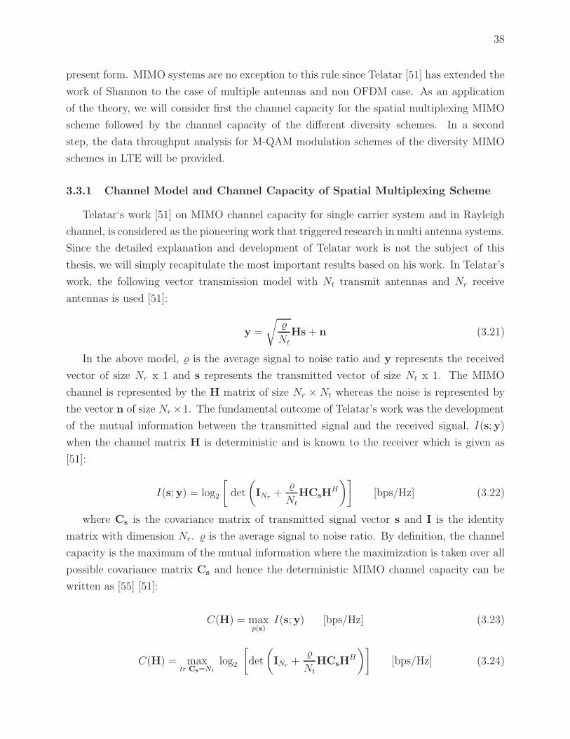
38

present form. MIMO systems are no exception to this rule since Telatar [51] has extended the

work of Shannon to the case of multiple antennas and non OFDM case. As an application

of the theory, we will consider first the channel capacity for the spatial multiplexing MIMO

scheme followed by the channel capacity of the different diversity schemes. In a second

step, the data throughput analysis for M-QAM modulation schemes of the diversity MIMO

schemes in LTE will be provided.

3.3.1 Channel Model and Channel Capacity of Spatial Multiplexing Scheme

Telatar‘s work [51] on MIMO channel capacity for single carrier system and in Rayleigh

channel, is considered as the pioneering work that triggered research in multi antenna systems.

Since the detailed explanation and development of Telatar work is not the subject of this

thesis, we will simply recapitulate the most important results based on his work. In Telatar’s

work, the following vector transmission model with Nt transmit antennas and Nr receive

antennas is used [51]:

y =

√

Nt

Hs + n (3.21)

In the above model, is the average signal to noise ratio and y represents the received

vector of size Nr x 1 and s represents the transmitted vector of size Nt x 1. The MIMO

channel is represented by the H matrix of size Nr × Nt whereas the noise is represented by

the vector n of size Nr×1. The fundamental outcome of Telatar’s work was the development

of the mutual information between the transmitted signal and the received signal, I(s;y)

when the channel matrix H is deterministic and is known to the receiver which is given as

[51]:

I(s;y) = log2

[det

(INr

+

NtHCsH

H

)][bps/Hz] (3.22)

where Cs is the covariance matrix of transmitted signal vector s and I is the identity

matrix with dimension Nr. is the average signal to noise ratio. By definition, the channel

capacity is the maximum of the mutual information where the maximization is taken over all

possible covariance matrix Cs and hence the deterministic MIMO channel capacity can be

written as [55] [51]:

C(H) = maxp(s)

I(s;y) [bps/Hz] (3.23)

C(H) = maxtr Cs=Nt

log2

[det

(INr

+

NtHCsH

H

)][bps/Hz] (3.24)

39

The above equation is known as the ”log-det” formula and is considered as the pioneering

work that triggered research in multi antennas systems. For fading channel, the channel

matrix H is a random matrix and hence the associated channel capacity is also a random

variable. To deal with the random behaviour of the channel, the average of the above equation

over the distribution of H with the given name of ergodic MIMO channel capacity can be

defined as [51]:

CE = E

{max

tr Cs=Nt

log2

[det

(INr

+

NtHCsH

H

)]}[bps/Hz] (3.25)

It is worth noting that the above derivation of the ergodic MIMO channel capacity does

not tell us how to choose the covariance matrix of s (Cs) to get the maximum mutual

information. To be able to compute the maximization, it should be clarified if the transmitter,

the receiver, or both have perfect knowledge of the channel state information (CSI).

If the channel matrix H is known at the transmitter, the transmit covariance matrix (Cs)

can be chosen to maximize the channel capacity for a given realization of the channel. The

main tool for performing this maximization is a technique known as water filling which we

will not consider in this thesis. If the channel matrix H is, however, known at the receiver,

Telatar showed that the optimal signal covariance matrix has to be chosen according to:

Cs = I (3.26)

This means that the antennas should transmit uncorrelated streams with the same average

power. With such covariance matrix, the ergodic MIMO channel capacity becomes [51]:

CE = E

{log2 det

(INr

+

Nt

HHH

)}[bps/Hz]. (3.27)

3.3.2 Channel Model and Channel Capacity of Diversity Schemes

The ergodic channel capacity in (3.27) is valid for channel matrix where different signals

are transmitted independently and hence cannot be applied directly to the space time block

coding where the signals are transmitted in the form of space block codes. In fact, a STBC

scheme with Nt transmit antennas and Nr receive antennas is generally characterized by the

40

transmission matrix which has general form [49]:

G =

g11 g21 ... gNt1

g12 g22 ... gNt2

. . ... .

. . ... .

g1T g2T ... gNtT

(3.28)

where gij represents a linear combination of the signal constellation components and their

conjugates. gij is transmitted from the ith transmit antenna in the jth time slot for i =

1, ..., Nt and j = 1, ..., T . T represents the number of time slots used to transmit S symbols.

For such STBC, it has been found that the equivalent AWGN scaled channel is given by [59]:

ynT

=1

Rc

‖H‖2FxnT +wnT (3.29)

where ynT

is the S × 1 complex matrix after STBC decoding and S represents the number

of transmitted symbols. xnT is the transmitted S× 1 complex vector with each entry having

energy Es/Nt, Es is the maximum total transmitted energy on the Nt transmit antennas per

symbol time, and wnT is complex Gaussian noise with zero mean and variance N0/2 in each

dimension. ‖H‖2F =∑N

i=1

∑Mj=1 ‖hij‖2 is the squared Frobenius norm of H, hij is the channel

gain from the ith transmit antenna to the j th receive antenna. Rc is the code rate of the

STBC and defined as S/T , where T is the number of time slots to transmit one block code.

From the equivalent AWGN channel in (3.29), it was shown that the effective instantaneous

SNR at the receiver denoted as γ is given as [59]:

γ =Es

NtRcN0‖H‖2F (3.30)

which means that the channel matrix is converted into a scalar channel [40] [31] [12] [59] and

hence the ergodic capacity of the equivalent STBC channel in (3.29) is given by [40] and [12]

as:

C = E [Rc log2(1 + γ)] (b/s/Hz) (3.31)

or equivalently, by inserting (3.30) into (3.31):

C = E

[Rc log2

(1 +

Es

NtRcN0‖H‖2F

)](b/s/Hz) (3.32)

If the probability density function of the instantaneous SNR p(γs) is known, the ergodic

41

capacity of the equivalent STBC can be evaluated using the following integral equation [40]:

C = Rc

∫ ∞

0

log2 (1 + γ) p(γs)dγs (b/s/Hz) (3.33)

Equation (3.33) represents the fundamental formula for capacity evaluation of any diver-

sity STBC scheme. This is through this equation that we will present our capacity analysis

of SFBC-OFDM and FSTD-OFDM diversity schemes in LTE environment.

SFBC Channel Capacity Analysis

Since OFDM system converts the multipath channel intoN frequency flat-fading subchan-

nels, the average capacity over flat-fading subchannel that is defined by Ck is determined first.

Then, the overall average channel capacity over N can be found as:

Cχ=

1

N

N∑

k=1

Cχ

k (3.34)

where k represents the subcarrier index and χ ∈ {SFBC, FSTD}. The average capacity

achieved by a SFBC-OFDM scheme is calculated using the probability density function of

the instantaneous SNR [52]:

CSFBC

k =

∫ ∞

0

Rc log2 (1 + γ)fSFBCγ (γ)dγ (3.35)

where fSFBCγ (γ) is defined as

fSFBCγ (γ) =

2

γ2γe−

2

γγ (3.36)

Substituting the PDF in the equation of average capacity, we obtain:

CSFBC

k =

∫ ∞

0

Rc log2 (1 + γ)2

γ2γe−

2

γγdγ (3.37)

After some manipulation, the equation of the CSFBC

k can be written as:

CSFBC

k = Aµ

∫ ∞

0

ln (1 + γ)(µγ)η−1e−µγdγ (3.38)

where

A =Rc × log2(10)× log10(e)

2; µ =

2

γ; η = 2 (3.39)

The integral in equation (3.38) can be evaluated using the following results [22]:

42

µ

(η − 1)!

∫ ∞

0

ln(1 + x)(µx)η−1e−µxdx = Pη(−µ)E1(µ) + Ση−1q=1

1

qPq(µ)Pη−q(−µ) (3.40)

where Pq(.) and E1(x) represent respectively the Poisson distribution and the exponential

integral of first order which are given as [22]

Pq(x) = Σq−1v=0(

xv

v!)e−x (3.41)

E1(x) =

∫ ∞

x

t−1e−tdt for x > 0 (3.42)

Using (3.40), the closed form of (3.38) becomes

CSFBC

k = A{P2(−µ)E1(µ) + P1(µ)P1(−µ)} (3.43)

This concludes our analysis for the 2× 1 SFBC scheme.

FSTD Channel Capacity Analysis

Following the same approach adopted for the analysis of 2 × 1 SFBC scheme, we can

determine the average channel capacity for the (4 × 2) FSTD scheme. To this end, we use

the expression for the kth OFDM subcarrier CFSTD

k [52]:

CFSTD

k =

∫ ∞

0

Rclog2(1 + γ)fFSTDγ (γ)dγ (3.44)

where fFSTDγ (γ) is defined by:

fFSTDγ (γ) =

8

3γ4γ3e−

2

γγ. (3.45)

Substituting (3.45) in (3.44), we obtain:

CFSTD

k =

∫ ∞

0

Rclog2(1 + γ)8

3γ4γ3e−

2

γγdγ (3.46)

which after some manipulation, becomes:

CFSTD

k =Aµ

3

∫ ∞

0

ln(1 + γ)(µγ)η−1e−µγdγ (3.47)

where A and µ are as defined in (3.39) and η = 4. Using (3.40), a closed form can be found

43

as:

CFSTD

k = 2A

[P4(−µ)E1(µ) + Σ3

q=1

1

qPq(µ)Pη−q(−µ)

](3.48)

This concludes our analysis of 4× 2 FSTD MIMO scheme in LTE. The numerical results

in terms of bits/s/Hz are shown in Figure 3.4. To verify our analysis, the results of Monte-

−10 −5 0 5 10 15 20 25 30 35 400

2

4

6

8

10

12

14

15

SNR (dB)

Ca

pa

city (

bp

s/H

z)

Theoretical Capacity SISOSimulation Capacity SISOTheoretical Capacity SFBC−OFDM 2x1Simulation Capacity SFBC−OFDM 2x1Theoretical Capacity FSTD−OFDM 4x2Simulation Capacity FSTD−OFDM 4x2

Figure 3.4 Capacity for SISO, SFBC-OFDM and FSTD-OFDM Schemes

Carlo simulation of channel capacity of the two studied diversity schemes as well as the

SISO case are also included. The dashed line curve in Figure 3.4 represents the channel

capacity of SISO scheme using our analysis. The diamond shaped points represents the SISO

capacity obtained with Monte-Carlo simulation. The theoretical channel capacity of 2 × 1

STBC is shown by the red curve in Figure 3.4, whereas the black square line represent the

capacity obtained by Monte-Carlo simulation. As expected, in the high SNR regions, only a

small improvement of the channel capacity of the 2 × 1 SBC with respect to the SISO case

is observed. Specifically, for SNR = 34 dB the improvement of 2 × 1 STBC is about 0.5

bits/s/Hz with respect to SISO. For low SNR regions, the channel capacity of the SISO case

and the 2× 1 STBC is almost the same. The theoretical channel capacity of the 2× 2 STBC

44

scheme is shown by the purple dashed line in Figure 3.4. The improvement with respect to

the SISO case is more important. In fact, for the same SNR = 34 dB, the improvement is

about 1.6 bits/s/Hz. Finally, it can be observed from Figure 3.4 that numerical evaluation

results obtained from capacity analysis match closely to the capacity results obtained from

Monte-Carlo simulations, which comforts us in the accuracy of our mathematical analysis.

3.4 Data Throughput Performance Evaluation for M-QAM Modulation Schemes

In SISO OFDM systems, the maximal data throughput depends on the available band-

width and the parameters associated with the OFDM signal, such as the number of subcarriers

and the modulation order (QPSK, 16-QAM, 64-QAM). For a given frequency bandwidth (B)

the maximal coded data throughput in bits per second can be approximated by the following

simple equation [32]:

CodedThroughput(bps) =NFB.NSC .NOFDM .Nb.ECR

Tsub(3.49)

where NFB is the number of Frequency Blocks in the given frequency bandwidth (B), NSC is

the number of subcarriers in one Frequency Block, NOFDM is the number of OFDM symbols

in one subframe, Nb is the number of bits in one subcarrier; ECR is the Effective Code Rate,

and Tsub is the duration of one subframe that is equal to 1 ms. In LTE, NSC and NOFDM are

fixed with values 12 and 14 respectively [4]. For 5 MHz (NFB = 25) bandwidth LTE system

with 64-QAM Modulation (Nb = 6) and ECR = 0.9, the maximal data throughput that can

be supported by the system is then 22.68 Mbps. The uncoded data throughput can be found

by excluding the effective code rate (ECR) from the equation (3.49). This yields:

UncodedThroughput(bps) =NFB.NSC .NOFDM .Nb

Tsub

(3.50)

The throughput results can be compared to the system capacity Cχ

B (χ ∈ {SFBC, FSTD})of a flat fading channel as developed in Section 3.3 but adjusted by the inherent system losses.

In this case, the system capacity is simply given as [32]:

Cχ

B = F × B × Cχ. (3.51)

where F and B are two correcting factors. The correcting factor B can be calculated as [32]:

B =NSC .NOFDM .NFB

Tsub

(3.52)

45

where NSC is the number of subcarriers in one Resource Block and is equal to 12, NOFDM

represents the number of OFDM symbols in one subframe and for normal cyclic prefix it

is equal to 14. NFB is the number of resource blocks (RB) that fit into the selected band-

width (for example in 5 MHz bandwidth we found 25 Resource Blocks). The values of NFB

corresponding to the selected bandwidth (B) are shown in Table 3.2.

Finally, Tsub is the duration of one subframe and is equal to 1 ms. To take into account

the losses due to the added cyclic prefix and reference symbols, a correction factor F is

introduced in the calculation of the system capacity and is given by [32]:

F =Tframe − Tcp

Tframe× Nsc ×NOFDM/2− 4

Nsc ×NOFDM/2(3.53)

where Tframe is the fixed duration frame and is equal to 10 ms. Tcp represents the total Cyclic

Prefix time of all OFDM symbols within one frame and is given by:

Tcp = (Tcp1 + 6× Tcp2)×Nslot (3.54)

where Tcp1 is the duration of the first cyclic prefix of the first OFDM symbol in one slot and

is equal to 5.2µs. Tcp2 is the duration of the cyclic prefix of the next six OFDM symbols in

one slot as shown in Figure 2.7 and is equal to 4.7µs. Finally, Nslot is the number of slots

within the duration of one frame and is equal to 20. The results of calculation of the system

capacity based on Equation 3.51 for different bandwidth values are shown in Figure 3.5.

CB = F × B × log2(1 + γ). (3.55)

The results in Figure 3.5 represent the limit of channel capacity of a system with con-

tinuous valued inputs and continuous valued outputs of complex signals for different channel

bandwidth (B) as defined in LTE (Table 3.2). These limits can be considered as an upper

Table 3.2 Number of Resource Blocks

B (MHz) NFB

1.4 65 2510 5015 7520 100

46

−10 −5 0 5 10 15 20 250

20

40

60

80

100

120

140

SNR (dB)

Syste

m S

ha

nn

on

Ca

pa

city (

Mb

ps)

1.4 MHz5 MHz10 MHz15 MHz20 MHz

Figure 3.5 System Capacity as a function of SNR for different Bandwidth settings

bound of real data throughput of a system with discrete valued multilevel/phase inputs. It

can also be noticed from the Figure how the Shannon capacity increases as the bandwidth

increases. The results relative to real data throughput and their respective limit will be

shown in the next section.

Table 3.3 ECR and Modulation Order for CQI

CQI Modulation ECR ECR x 1024[6]1 4QAM 0.0762 782 4QAM 0.1172 1203 4QAM 0.1885 1934 4QAM 0.3008 3085 4QAM 0.4385 4496 4QAM 0.5879 6027 16QAM 0.3691 3788 16QAM 0.4785 4909 16QAM 0.6016 61610 64QAM 0.4551 46611 64QAM 0.5537 56712 64QAM 0.6504 66613 64QAM 0.7539 77214 64QAM 0.8525 87315 64QAM 0.9258 948

47

Table 3.4 SISO Generated Data

Modulation Scheme QPSKMIMO Configuration SISO 2× 1 SFBC 4× 2 FSTD

ECR 0.5879 0.6016 0.9258Max Possible Data (Bits/SubFrame) 8400 8400 8400

Tx Data bits1st SubFrame 4512 4372 4136

2nd to 5th SubFrames 4680 4456 4220

Tx Coded Bits1st SubFrame 7712 7456 7056

2nd to 5th SubFrames 8000 7600 7200

Tx User Symbols1st SubFrame 3856 3728 35282nd to 5th SubFrames 4000 3800 3600

Expected Data Throughput (Bits/Subframe) 8000 7600 7200Calculated ECR 0.5850 0.5863 0.5861

3.4.1 Numerical Results and Discussion for System Throughput

In this section, we present numerical results of the data throughput results of SFBC-

OFDM and FSTD-OFDM MIMO schemes for different M-QAM modulation schemes using

the LTE simulator [36]. The LTE simulator allows the calculation of coded and uncoded data

throughput. For coded calculations, the transmitted signal is coded using the Turbo Code as

defined in LTE. The overall effective code rates for different modulation schemes are defined

in LTE and are given in Table 3.3. The Monte-Carlo simulation results are presented in the

Figure 3.6; 3.7 and 3.8, where they are compared to coded and un-coded data throughput for

the SISO configuration. Figure 3.6 represents the results for QPSK modulation. The results

of 16-QAM are presented in Figure 3.7 while those relative to 64-QAM modulation appear

in Figure 3.8.

For QPSK modulation, the un-coded data throughput of SISO configuration is shown by the

ball blue curve. It can be observed that as the SNR increases the data throughput increases

and it reaches its maximum at an SNR of almost 48 dB. The coded data throughput of

the same modulation (QPSK) and represented by the blue curve in Figure 3.6 reaches its

maximum with only 10 dB. As expected from the coding process, the coded data throughput

is less than the un-coded data throughput. In fact, the coded and un-coded data throughputs

are related by the effective code rate used for channel coding. As shown in Table 3.3, the ECR

for QPSK (CQI = 6) is equal to 0.5879, which represents the ratio of the useful transmitted

data rate to the overall coded data after channel coding. An ECR of 0.5879 means that

only 0.5879 of the transmitted data are useful data. The remaining data are used only for

error protection and detection. This principle is well represented in the results of Figure

3.6, where the coded data throughput is found to be 4.9 Mbps whereas the un-coded data

throughput is 8.3 Mbps, which represents, effectively and as expected, a code rate of 0.5879.

The benefits of using the channel coding (Turbo coding in LTE)is clearly shown in Figure

48

−10 0 10 20 30 40 50 600

1

2

3

4

5

6

7

8

9

SNR (dB)

Th

rou

gh

pu

t (M

bp

s)

Capacity Limit SISO

Capacity Limit 2x1

Capacity Limit 4x2

Coded SISO

Coded SFBC 2x1

Coded FSTD 4x2

Uncoded SISO

Uncoded SFBC 2x1

UnCoded FSTD 4x2

Un−Coded

Coded

Capacity Limit

Figure 3.6 Data Throughput for QPSK Modulation

3.6, where the data throughput of coded scheme is much closer to the channel capacity limit.

The coded and un-coded data throughput of the 2 × 1 SFBC are represented by the green

and purple curves respectively. In case of un-coded scheme, the improvement with respect

to the SISO case is more significant and substantial as shown in Figure 3.6. However, for

coded case, there is no big difference between SISO and 2× 1 scheme and the improvement

is less significant. One last interesting observation from the results in Figure 3.6 is the fact

that at high SNRs the SISO data throughput is greater than the data throughput for 2 × 1

and 4× 2 diversity schemes. This result is explained by the fact that more overhead data is

transmitted in case of diversity schemes as shown in Table 3.4. Specifically, for SISO scheme

the symbol rate is 4000 per subframe (1 ms) whereas with 2× 1 SFBC case, the symbol rate

is 3800 per subframe. The symbol rate of 4 × 2 FSTD is the smallest one and is found to

be 3600 per subframe and that is why the data throughput of 4 × 2 FSTD is the smallest

one at the high SNR region as shown in Figure 3.6. This observation is valid for both coded

and un-coded data throughput. The red and citrine curves represent the coded and un-coded

data throughput respectively for the 4× 2 FSTD diversity scheme. Same observations as for

2×1 SFBC scheme can be made here. The theoretical channel capacity limits for SISO, 2×1

49

SFBC and 4 × 2 FSTD in a Rayleigh channel are also shown in Figure 3.6 for illustration

and to show the effect of channel coding. It is clearly perceptible that the data throughput

comes closer to the capacity limit with using channel coding.

For 16-QAM modulation (Figure 3.7), which corresponds to a CQI of 9, the code rate

−10 0 10 20 30 40 50 600

2

4

6

8

10

12

14

16

18

SNR (dB)

Th

rou

gh

pu

t (M

bp

s)

Capacity Limit SISO

Capacity Limit 2x1

Capacity Limit 4x2

Coded SISO

UnCoded SISO

Coded SFBC 2x1

UnCoded SFBC 2x1

Coded FSTD 4x2

UnCoded FSTD 4x2

Coded

Un−Coded

Capacity Limit

Figure 3.7 Data Throughput for 16QAM Modulation

is 0.6016 (Table 3.3) and hence the un-coded data throughput is higher than the coded

data throughput. For SISO scheme, the maximum un-coded and coded data throughput,

represented by the ball blue and blue curves in Figure 3.7, are found to be 15.8 Mbps and

9.5 Mbps respectively, which corresponds as expected to a 0.6 (9.5/15.8) code rate. The

maximum data throughput is achieved with a SNR of 60 dB in case of un-coded scheme

whereas only 20 dB is needed to achieve the maximum of data throughput for coded scheme.

It can be observed from Figure 3.7 that the best performance in terms of data throughput

is achieved with the 4× 2 FSTD scheme where the maximum data throughput is reached at

SNR = 10 dB. To attain the maximum in 2× 1 SFBC scheme an SNR of 16 dB is required.

For SISO scheme an SNR of 20 dB is needed to achieve the maximum data throughput.

These results demonstrate the benefits of the diversity schemes. The code rate for CQI 15

(64-QAM Modulation) is 0.9258 which is close to 1. The maximum un-coded and coded

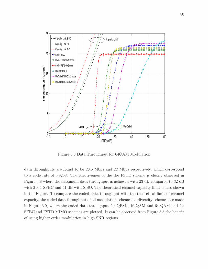
50

−10 0 10 20 30 40 50 600

5

10

15

20

25

SNR (dB)

Th

rou

gh

pu

t (M

bp

s)

Capacity Limit SISO

Capacity Limit 2x1

Capacity Limit 4x2

Coded SISO

Coded SFBC 2x1 Mode

Coded FSTD 4x2Mode

UnCoded SISO

UnCoded SFBC 2x1 Mode

UnCoded FSTD 4x2Mode

Coded Un−Coded

Capacity Limit

Figure 3.8 Data Throughput for 64QAM Modulation

data throughputs are found to be 23.5 Mbps and 22 Mbps respectively, which correspond

to a code rate of 0.9258. The effectiveness of the the FSTD scheme is clearly observed in

Figure 3.8 where the maximum data throughput is achieved with 23 dB compared to 32 dB

with 2× 1 SFBC and 41 dB with SISO. The theoretical channel capacity limit is also shown

in the Figure. To compare the coded data throughput with the theoretical limit of channel

capacity, the coded data throughput of all modulation schemes ad diversity schemes are made

in Figure 3.9, where the coded data throughput for QPSK, 16-QAM and 64-QAM and for

SFBC and FSTD MIMO schemes are plotted. It can be observed from Figure 3.8 the benefit

of using higher order modulation in high SNR regions.

51

−10 −5 0 5 10 15 20 25 30 35 400

5

10

15

20

25

SNR (dB)

Co

de

d D

ata

Th

rou

gh

pu

t (M

bp

s)

Capacity Limit SISOCapacity Limit 2x1Capacity Limit 4x2SISO QPSKSFBC 2x1 QPSKFSTD 4x2 QPSKSISO 16QAMSFBC 2x1 16QAMFSTD 4x2 16QAMSISO 64QAMSFBC 2x1 64QAMFSTD 4x2 64QAM

64−QAM

16−QAM

QPSK

Capacity Limit

Figure 3.9 Coded Data Throughput for M-QAM Modulation

52

CHAPTER 4

ANTENNA SELECTION IN MIMO SYSTEMS

As discussed in Chapter 3, the MIMO systems using multiple antennas at the transmit-

ter and multiple antennas at the receiver can improve significantly the system data rates

and reliability. The data rate improvement is achieved by the simultaneous transmission of

multiple streams of data using spatial multiplexing techniques. For channels with no spatial

correlation, the data rate can increase linearly with the minimum number of transmit and

receive antennas (min (Nr, Nt). A popular example of spatial multiplexing technique is the

V-BLAST suggested by Foschini [15]. The improvement in reliability is achieved through the

use of space diversity to significantly reduce the deep fades probability of a channel. In 1998,

Alamouti has designed a simple transmit diversity scheme with two transmit antennas [5].

Alamouti’s method provides a full diversity and requires simple linear operations both at the

transmit and receive sides. The processes of coding and decoding are performed in blocks of

transmitted symbols. Using the theory of orthogonal designs, the simple transmit diversity

technique of Alamouti has been generalized for a number of transmit antennas greater than

two [50] to a family of transmit diversity schemes known as Orthogonal Space-Time Block

Codes (OSTBC). As a different approach, Space-Time Trellis Codes (STTC) are also used

as transmit diversity schemes in MIMO systems. Also, OSTBC are the simplest space-time

codes that exploit the diversity offered by multiple antennas MIMO systems.

Besides the above mentioned advantages, MIMO systems have also some drawbacks. One

of the main drawback in the developments of MIMO systems is the increased cost caused by

the implementation of multiple Radio Frequency (RF) chains. For example, a Nr×Nt MIMO

system requires on the receiver side Nr low noise amplifiers, Nr analog to digital converters as

well as Nr RF to Intermediate Frequency (IF) converters and Nt digital to analog converters,

and on the transmitter side Nt RF amplifiers and Nt IF to RF converters to be implemented

which leads to high costs for the implementation of MIMO systems. To remedy this problem,

MIMO systems with antenna selection have been proposed, where the number of available

antennas at the receiver (Nr) is greater than the number of implemented RF chains (Lr).

The antenna selection scheme has been studied and used for a long time in the context of

radio links at the receiver with a single antenna at the transmitters. In the literature, this

technique is known as Selection Combining (SC) and Hybrid Selection/MRC (H-S/MRC). In

the SC technique, one receive antenna is selected out of Nr antennas whereas in HS/MRC Lr

53

antennas are selected fromNr receive antennas. For the case of a MIMO system in general, the

use of the antenna selection technique is known as the Hybrid Selection/MIMO (HS/MIMO).

Using a predefined selection criterion, several (Lr ≤ Nr) among the Nr receive antennas can

be selected. Thus, one can use a limited number of RF chains which are allocated to the best

Lr antennas. Obviously, this significant reduction in the complexity of the implementation

is not without price. In fact, it is at the expense of a loss, relatively small, in the system

capacity compared to the MIMO system using all antennas.

This chapter is organized as follows. In Section 4.1, we provide a brief literature overview

of the theory of antenna selection in MIMO systems and its impact on the performance

of these systems and more specifically, the impact on the channel capacity and the Bit

Error Rate. A detailed description of main antennas selection algorithms is also provided in

this section. In section 4.2, some results of the impact of the implemented Un-Correlated

Based Selection (UCBS) algorithms are provided. In section 4.3, we present the analysis

of the performance of MIMO systems using antennas selection techniques in non correlated

channels. Finally, in section 4.4, we evaluate the impact of antenna correlation on the BER

performances of MIMO OSTBC with receive antennas selection.

4.1 Antenna Selection Overview

MIMO systems with antenna selection have been extensively studied in various literatures

[17], [9], [18], [34]. In [34], the authors study the capacity upper bound of MIMO systems

with antenna selection on the receiver side. In particular they demonstrate that the capacity

is very close to that of a system without selection if the number of receive antennas is greater

or equal than the number of transmit antennas. The authors in [17] investigate the capacity

of MIMO systems with antenna selection in the case when the rank of the channel matrix is

low. Based on the minimization of the probability of error per symbol (SER ), the authors

[9] and [18] present an antenna selection scheme for space-time block coding systems. In

[18], the authors study the performances of joint transmit and receive antenna selection for

the cases of exact channel knowledge (ECK) and for statistical channel knowledge (SCK).

For ECK case, they consider the specific Alamouti code [5], whereas the more general space

time coding is considered for the SCK case. In their analysis, they adopt a selection criterion

that maximizes the Frobenius norm of the channel and, accordingly, they derive expressions

showing improvement in the signal to noise ratio (SNR) and in the outage capacity. They

use the outage capacity to affirm that the spatial diversity using the space time block coding

is maintained by the antenna selection. This impact is also analyzed in [58]. In their analy-

sis, an upper bound on the performance of BER systems with antenna selection is explicitly

54

derived. They demonstrate that the diversity order of a system with antenna selection is the

same as that of the system using all available antennas. In addition, they derive a tight upper

bound for the performance of the bit error rate (BER) for a system with Nr receive antennas

Nt transmit antennas and Lr = 1. An expression for the BER performance of Alamouti code

has also been developed when Lr = 1. In [24] , Heath et al. propose a criteria for selecting an

optimal antenna of subset that minimize the error rate. In their studies, they use coherent

receivers such as liner or maximum likelihood (ML) over a slowly varying channel. Several

selection algorithms, geared at maximizing the channel capacity were presented by different

authors [19] − [10]. In [27], the authors consider an antenna selection on the transmitter

side for OSTBC codes. Through Monte-Carlo simulations, they demonstrate that under the

assumption that the number of selected antennas is fixed, the performance is improved when

the number of available transmit antennas is increased. [54] consider the selection of antennas

for MIMO systems using three transmit antennas and a single receive antenna. They intro-

duce an algorithm to select the two best antennas based on the channel statistics provided

by the receiver. A complete review of the literature on antenna selection in MIMO systems

can be found in [33].

The optimal choice in antenna selection requires the knowledge and the estimation of the

full channel MIMO matrix. To perform the estimation of all antennas, it seems necessary to

make available all the Nr RF chains, which goes against the goal of reducing the number of

RF chains. However, in an environment that changes sufficiently slowly and with the help of

a training sequence, antennas can be multiplexed to different RF chains so that the channel

is estimated successively antenna by antenna. Practically a RF receive chain is connected to

the first receive antenna during the first part of the training sequence to estimate the channel

seen by the first antenna. Then the same chain is connected to the second antenna in the

second part of the training sequence to estimate the channel of the second antenna. This

procedure is then repeated for all available antennas. This allows the determination of the

channel state information (CSI) in all antenna elements (Nr). At the end of the training

sequence, the channels of all antennas are estimated and based on that estimation, the best

Lr antennas are selected . Therefore, a few more bits of training sequence are needed instead

of additional RF channels. In a system with high data rate, such additional bits do not affect

the spectral efficiency significantly.

In this chapter, we consider a MIMO system equipped with Nt transmit antennas and Nr

receive antennas as shown in Figure 4.1. In addition, we suppose that the transmitter has Lt

radio frequency (RF) chains and the receiver has Lr RF chains, where Lt < Nt and Lr < Nr,

55

Figure 4.1 MIMO system Model with Antenna Selection

as indicated in Figure 4.1. When there is no antenna selection, Lt = Nt and Lr = Nr.

Referring to Figure 4.1, we can distinguish three types of antenna selection mechanisms:

1. Receive Antenna Selection (RAS)

2. Transmit Antenna Selection (TAS)

3. Joint Transmit-Receive Antenna Selection (TRAS)

In case of Receive Antenna Selection, we have Lt = Nt. The goal of a Receive Antenna

selection algorithm is to find the optimal subset of receive antennas that maximizes some

selection criteria. This is what is called the optimal receive antenna selection. The only

mechanism for an optimal receive antenna selection is to make an exhaustive search among

all possible combinations and find the antennas subset that maximizes the selection crite-

rion. It follows that an optimal receive antenna selection necessitates a prohibiting time of

computation for the evaluation of the selection criteria(

Nr

Lr

)

times. For Transmit Antenna

Selection, we have Lr = Nr and the optimal transmit antenna selection necessitate the evalu-

ation of the selection criteria(

Nt

Lt

)

times. Finally, for joint transmit-receive antenna selection

a total of(

Nt

Lt

)(

Nr

Lr

)

evaluation of the selection criteria is needed. Usually, the selection

criteria goal is to maximize the channel capacity or minimize the BER.

Based on the system model in Figure 4.1, the received signal at an instant index time n

is given by:

y[n] = Hx[n] + n[n], (4.1)

56

where H is a Nr ×Nt matrix

H =

h11 h12 · · · h1Nt

h21 h22 · · · h2Nt

......

. . ....

hNr1 hNr2 · · · hNrNt

, (4.2)

where the element hij represents the channel transfer coefficient between transmitter j and

receiver i. x[n] is the transmitted vector of size (Nt×1) at instant time n and n[n] represents

the vector of additive white gaussian noise (AWGN) of size Nr × 1. The elements hij,

of the matrix H are complex gaussian random variables with zero mean and 0.5 variance

per dimension. The elements of n[n] are random gaussian variables with zero mean and

N0/2 variance per dimension. Only otherwise stated, it is assumed that all the channels

are independent and the channel state information (CSI) is perfectly known at the receiver,

but not at the transmitter. In a quasi static fading channel, the channel coefficients are

considered constant during one frame but they change independently from frame to frame.

In a block fading channel, the channel coefficients are considered constant during one block

of symbols, but they change independently from one block to another. In both cases, the

channel is considered a non-frequency selective channel (Flat-fading channel). This is the

case when the coherence bandwidth of the channel is much larger than the bandwidth of the

transmitted signal. We consider the following two main selection criteria which maximize the

channel capacity and maximize the SNR.

4.1.1 Antenna Selection Scheme based on the Channel Capacity

When the channel state information is not known at the transmitter, which is the case for

many situations, the transmitted power should be distributed equally through all transmitted

antennas. Hence, the signal to noise ratio (SNR) in each receive antenna is given by [13]:

ρ.=

P

NoB, (4.3)

where P is the total transmitted power and B is the transmitted bandwidth. If we define the

ratio γ.= Eb/No, where Eb is the average energy per transmitted bit, the relation between ρ

and γ is then given by:

γ =ρ

R, (4.4)

57

where R represents the information transmitted rate in bits/s/Hz. The channel capacity of

MIMO system using all antennas at the transmitter and at the receiver sides (no-selection)

is given by [13]:

C = log2

[det

(INr

+ρ

NtHH†

)]. (4.5)

.

In [33], it was shown that in receive antenna selection, when the receiver selects the best

Lr antennas out of Nr antennas that maximize the channel capacity in (4.5), the channel

capacity of the selected channel matrix is upper bounded by:

Cselect ≤Lr∑

i=1

log2

(1 +

ρ

Ntγi

), (4.6)

where γi represents the squared norm of the ith line of the matrixH, after ascending ordering.

Hence, γi are ordered random variables with a Chi-square distribution. This upper bound is

tight enough for Lr < Nr. It was also shown that the channel capacity of MIMO systems

is maintained provided that the number of selected antennas in one side is at least equal to

the number of available antennas at the other side. While the antenna selection maintains

the majority of the promised capacity by MIMO systems, the computation level due to the

selection algorithm complexity is quite large because there are(

Nr

Lr

)

possibilities for selection

from each side. In order to reduce the computation complexity, many sub-optimal antenna

selection algorithms have been proposed with no extensive loss in capacity compared to

optimal selection [33]. When the transmission data rate is larger than the instantaneous

mutual information, an outage event appears. In a quasi static fading chanel, where the

channel coefficients are constant during all the frame, it is not possible to quantify with an

average measure. In such situation, the Shannon capacity is essentially a random variable.

The probability of such event is known as outage probability. This probability for high SNR

regions, when the best Lr receive antennas are selected, is upper bounded by [46]:

Pselect ≤ koγ−NtNr , (4.7)

where

ko =

(2R−1R

(Nr

Lr

)NrNt

)NrNt

(NtNr)!, (4.8)

58

We can see from Equation (4.7) that the diversity order, expressed by the NtNr exponent, is

the same for a MIMO system without antenna selection (Lr = Nr) and for a MIMO system

with receive antenna selection (Lr < Nr), and this is true for any value of Nr, Nt, and Lr.

However, this expression cannot be used to quantify the outage probability, simply because

the upper bound gap is large. For that reason, the authors of [46] used another expression to

quantify the degradation of the SNR (ρ) due to receive antenna selection. This expression is

given by [46]:

Pselect ≤ Pr

(Nr∑

i=Nr−Lr+1

Xi:Nr≤(2R/Lr − 1

) NtLr

ρδ

), (4.9)

where δ = 10ζ/10, Xi:Nrrepresents the diagonal elements of the matrix HHH after ordering

(random variables with Chi-Square distribution with 2N degrees of freedom) and ζ represents

the maximum deviation between the lower bound and the exact value of outage probability.

This deviation is expressed by [46]:

ζ = 10 log10

[2R

(2R/Nr − 1)Nr

(Nr − 1

Nr

)Nr−1]. (4.10)

Equation (4.10) represents an approximation of the degradation of the SNR due to antennas

selection.

4.1.2 Antenna Selection Scheme based on the SNR

The antenna selection based on the instantaneous signal to noise ratio (SNR) is more

attractive because it is more practical than the one based on the maximization of channel

capacity. In the following, we consider the impact of receive antenna selection for MIMO

systems using the orthogonal space time block coding (OSTBC). Many upper bounds of the

probability of bit error rate (BER) of OSTBC have been derived in [58], for an arbitrary

number of transmit antennas and receive antennas as well as arbitrary number of selected

antennas. In case of BPSK constellation and Maximum Likelihood Decoding (MLD), the

probability of error per bit of a MIMO system without selection, for high SNR, is approxi-

mated by [39]:

Pb(e) ≈(

2NtNr − 1

NtNr

)(4Es

N0

)−NtNr

, (4.11)

where Es is the average energy per transmitted symbol, and N0/2 is the variance (per di-

mension) of the complex additive white Gaussian noise (AWGN). It clearly shows that the

59

diversity order is NtNr. In [58], it was shown that when the best Lr antennas were selected

among Nr antennas, the probability of error is approximated by:

Pb(e) ≈(

2NtNr − 1

NtNr

)(4Lr

Nr

Es

N0

)−NtNr

. (4.12)

.

Comparing equation (4.11) with (4.12), we can conclude that, for Lr < Nr, the diver-

sity order does not change with antenna selection compared to MIMO system using all the

antennas. In addition, it is easy to notice that the SNR reduction due to receive antenna

selection is upper bounded by 10log10(Nr/Lr) dB. In [58], an exact bound was derived when

the receiver selects the best antennas.

4.1.3 Antenna Selection Algorithms

Many algorithms for antenna selection have been published in the literature [10], [37],

[56], which can be classified as receive antennas selection, transmit antenna selection or

joint transmit-receive antenna selection. Furthermore as discussed earlier, antenna selection

algorithms can also be classified based on the selection criterion such as:

– selection based on the maximization of channel capacity (C)

– selection based on the minimisation of error probability (BER)

Antenna selection algorithms that minimize the bit error probability will necessarily min-

imize the pairwise error probability (PEP) and the union bound. The minimization of the

bit error probability leads necessarily to maximizing the instantaneous signal to noise ratio.

On the other hand, maximizing the capacity does not lead to maximizing the signal to noise

ratio. Intuitively, maximizing capacity and maximizing the signal to noise ratio appear to

be equivalent. But this is not always the case in theory. In fact, antenna selection based

on maximizing the SNR does not lead necessarily to channel capacity maximization. This

is attributed to the fact that the capacity is much more affected by the phase difference

between the antenna elements than the instantaneous signal to noise ratio. On the other

hand, maximizing the received SNR leads, necessarily, to the minimization of the BER. It

then follows that the algorithms based on the SNR maximizing are equivalent to those based

on minimization of the BER. In what follows, we present the different algorithms for antenna

selection.

60

Norm Based Selection Algorithm (NBS)

The simplest algorithm for antenna selection is known as Norm Based Selection (NBS)

[18]. The principle of the algorithm is to select the receive antennas subset that maximize

the Frobenius norm of the channel. This method does not require too much computation,

but does not provide a good performance. The algorithm was developed for systems using

orthogonal space-time block coding (OSTBC), particularly the Alamouti coding [18]. The

choice of the Frobenius norm as a selection criterion is motivated by the fact that the signal

to noise ratio and, therefore, the probability of error, depend on the Frobenius norm. In fact,

for OSTBC systems, the received signal to noise ratio is given by [5]:

γ = γo‖H‖2F , (4.13)

where γo = Es/(NtNo) and ‖H‖2F is the Frobenius norm of the matrix H defined by:

‖H‖2F =

Nr∑

i=1

Nt∑

j=1

|hij |2. (4.14)

where hij represents the elements of the channel matrix H as defined in section 4.1. The

symbol probability error Pe is then upper bounded by [18]:

Pe ≤ e−dγo‖H‖2F , (4.15)

where d is a constant that depends on the modulation order. From equations (4.15) and

(4.13), it is clear that maximizing the Frobenius norm inevitably leads to maximizing the

SNR and at the same time minimizing the instantaneous probability of error. For this

algorithm, two analyzes have been developed to quantify the performance [18]. The first

analysis is based on the average signal to noise ratio. This analysis is general and can be

applied to any orthogonal space time block codes. The second analysis focuses on the outage

probability. The capacity analysis is limited to the case of a transmit selection with Alamouti

coding. Following this analysis, the antenna selection gain in terms of the average signal to

noise ratio is expressed by [18]:

g = log10

( E{γ}γoLrLt

)= log10

(E{∑i=1...Lt

Tni

2}LrLt

), (4.16)

61

where γoLrLt is the signal to noise ratio (SNR) for the orthogonal space time codes without

antennas selection and E{γ} is the average signal to noise ratio for orthogonal space time

codes with antenna selection given by [18]:

E{γ} = γoE{‖H‖2F} = γo

Nt∑

i=1

E{T 2ni}, (4.17)

where Tk (k = 1, 2, ..., Nt) is the Frobenius norm of the Nt columns of the channel matrix H.

In [18], the gain (Equation (4.16)), g, is found to be substantial.

Correlation Based selection Algorithm (CBS)

Although the NBS algorithm is simple and straightforward to implement, its major draw-

back is that it does not provide a good performance. An alternative to this algorithm has

been proposed in [10]. This method is based on the correlation between the lines of the

channel matrix. The method is to find two lines with a strong correlation and then delete the

one having low power. This process is repeated until (Nr − Lr) lines are eliminated. With

this algorithm, it is possible to get Lr lines with a minimum of correlation and maximum

power.

Optimal Selection

The capacity of a (Nt ×Nr) MIMO system using all antennas is given by [10]:

Cfull = log2

[det

(INr

+Γ

NtHH†

)], (4.18)

where INris the identity matrix of size (Nr × Nr), Γ is the signal to noise ratio per MIMO

branch and the sign † indicate the Hermitian transpose. After receive antenna selection of

Lr antennas that maximize the channel capacity, the equation in 4.18 becomes:

Cselect = maxS(Hw)

(log2

[det

(ILr

+Γ

Nt

HwH†w

)]), (4.19)

where Hw is obtained by deleting (Nr − Lr) rows of the original matrix H and S(Hw)

represents the set of all possible Hw. The optimal antenna selection necessitates the calcu-

lation of(

Nr

Lr

)

determinants, which is time consuming. For this reason, authors presented a

62

sub-optimal algorithm allowing the reduction of complexity calculation [10].

Sub-Optimal Selection

The sub-optimal algorithm proposed by the authors [10] is based on the following equality:

det

(ILr

+Γ

NtHwH†

w

)=

r∏

k=1

(1 +

Γ

Ntλk

2

), (4.20)

where r represents the rank of the channel matrix and λk are the singular values of Hw. The

rank and the singular values should then be maximised in order to maximize the capacity.

When two rows (hk and hl) of the matrix H are identical, one of these two rows can be

eliminated. The power of each row (‖hk‖2) is also calculated in order to select the row with

highest power. If two rows have different powers, the row with the highest power is selected

and the other is rejected. Where there are no identical rows in the matrix, the rows with

high correlation are deleted. In this manner, we obtain a matrix Hw having low correlated

rows and with higher power.

The algorithm from [10] is the following:

1. The channel vector hk is defined as the k − th row of the matrix H, where k is an

element of the set X = {1, 2, ...., Nr}.2. for all k and l (k, l ∈ X), k > l, calculate the correlation Ξ(k, l). The correlation Ξ(k, l)

is defined as Ξ(k, l) = |〈hk, hl〉|.3. Loop

a) Choose the l (with k, l ∈ X, k > l) that give the largest correlation Ξ(k, l).

b) if ‖hk‖2 > ‖hl‖2, eliminate hl, otherwise, eliminate hk. Delete l (or k) from X .

c) repeat steps a) and b) until Nr − Lr rows are eliminated.

Un-Correlated Based Selection Algorithm (UCBS)

One of the disadvantages of the CBS algorithm is that it requires the computation of

the correlation of all the rows of the channel matrix. In addition, it creates a lot of loss

in capacity compared to the optimal selection. To overcome these drawbacks, the authors

of [37] presented a new algorithm and made changes to the CBS algorithm to improve its

performance in terms of capacity.

63

The UCBS algorithm is intended only for the receive antenna selection. The receiver has

Lr receive antennas and Nr RF receive chains, where LR < Nr. At the transmitter side, the

number of antennas and RF chains are equal (Nt = Lt). The goal of the UCBS algorithm is

to maximize the channel capacity. It is an algorithm that is based on the norm and the non-

correlation between the rows of channel matrix. The algorithm considers a MIMO system

equipped with Nt antennas at the transmitter and Nr antennas at the receiver. The channel

is assumed to be quasi-static with a non-frequency selective Rayleigh fading. In this case,

the input-output relationship of the MIMO system can be expressed as [37]:

y =

√ρ

Nt

Hx+ n, (4.21)

where y is an (Nr×1) received vector, x represents the transmitted vector of size (Nt×1), n is

an additive white gaussian noise (AWGN) with (No/2) per dimension, ρ is the average signal

to noise ration at each receive antenna and H is the MIMO channel matrix of size (Nr ×Nt).

The channel is supposed to be perfectly known at the receiver but not at the transmitter

side. The expression of the MIMO channel capacity when the channel state information is

not available at the transmitter can be given by [51]:

C(H) = log2

[det

(INt

+ρ

NtH†H

)], (4.22)

C(H) = log2

[det

(INr

+ρ

Nt

HH†)]

, (4.23)

where INris the Nr ×Nr identity matrix, (.)† represents the Hermitian transpose, and det(.)

is the matrix determinant.

The principle of the selection algorithm is to select the best Lr receive antennas among

Nr available based on the capacity maximization. We denote by w the subset of indices of

selected antennas (Example: w = {2, 3, 5} means that the second, third and fifth antennas

have been selected). The channel matrix corresponding to the selected antennas w is denoted

by Hw. With these notations, the channel capacity is determined by:

C(Hw) = log2

[det

(ILr

+ρ

NtHwH

†w

)], (4.24)

64

The purpose of selection algorithm is to find the matrix Hw that maximizes the channel

capacity C(Hw). The optimal selection method is an exhaustive search of all possible combi-

nations to find the antennas set that provides the maximum channel capacity. However, this

requires the computation of(

Nr

Lr

)

determinants for each channel realization. To illustrate

this method, consider the case of a system where we want to select two antennas among the

eight available antennas. In this case, the optimal method requires computation of:

(Nr

Lr

)=

(8

2

)=

8!

2! . (8− 2)!= 28 (4.25)

determinants. It is clear that the computational complexity becomes very large. This is

the reason for the interest in the development of sub-optimal antenna selection algorithms.

The idea behind the UCBS algorithm is to determine the matrix Hw by providing easier

computations than the required determinants. To this end, the matrix Hw is decomposed

into singular values (SVD). The channel capacity in terms of singular values decomposition

is then given by [37]:

C(Hw) =r∑

j=1

log2

[det

(ILr

+ρ

Nt

|λj (Hw)|2)]

, (4.26)

where r is the rank of the channel matrix Hw and λj (Hw) represents the jth singular value

of the matrix (Hw). Based on Equation (4.26), we can notice that to maximize the channel

capacity C(Hw), it is imperative to maximize the singular values (λj) and the rank (r) of

the matrix Hw. The problem becomes then to find the matrix Hw that has un-correlated

rows and maximum norm.

The UCBS algorithm is based on two parameters, namely αi,j and βi,j, defined in the

following way [37]:

αi,j =|hihj

†|‖hi‖‖hj‖

, (4.27)

βi,j =√1− αi,j

2, (4.28)

where hi represents the ith row of the channel matrix H et ‖.‖ is the vector Euclidian norm.

The value of αi,j represents the correlation between the ith and jth rows of the channel matrix

H. Consequently, βi,j corresponds to the non-correlation between ith row and jth row of the

channel matrix H. The proposed selection algorithm adopts an incremental procedure. The

65

procedure begins with an empty set of selected antennas. In each step of the algorithm, one

antenna is added to this set. Thereby, as the first step, the row with high Euclidian Norm is

selected. In the next step, the two parameters in equations (4.27) and (4.28) are calculated

with respect to the selected antenna in the first step for all remaining antennas. The antenna

that maximize a cost function fn,j is then selected and added to the selected antenna in the

first step. The cost function of the jth row is defined as follow:

fn,j =

{‖hj‖2, if n = 1

‖hj‖2∑n−1

m=1 β2wm,j if n ≥ 2

(4.29)

where wm is the mth selected antenna index. Hence, at each step, the selection rule is to find

the index wm of the receive antenna that maximizes the cost function fn,j, i.e.

wn = arg maxj∈Sn

fn,j, (4.30)

where Sn is the set of indices of receiving antennas which have not been selected in the

previous step. The procedure ends when all necessary antennas are chosen. Thus, the

proposed algorithm provides Lr receive antennas corresponding to the rows with a minimum

of correlation between them and having the maximum power.

Selection of two Rx antennas:

We Consider the specific case of selecting two antennas (Lr = 2). The Hw channel matrix

that maximize the channel capacity is found as follows:

Hw = argmaxHw

[log2

[det

(ILr +

ρ

NtHwHw

†)]]

= argmaxHw

[det

(ILr +

ρ

NtHwHw

†)]

. (4.31)

For high SNR values, the equation (4.31) can be approximated by:

Hw ≈ argmaxHw

[det

(ρ

NtHwHw

†)]

= argmaxHw

[det(HwHw

†)] . (4.32)

.

66

Table 4.1 UCBS Selection Algorithm

1 S = {1, 2, 3, ..., Nr}2 for j = 1 to Nr3 βj

2 = 04 γj = ‖hj‖5 end6 w = arg max γj

2

7 for n = 2 to Lr

8 S = S − {w}9 for all j ∈ S

10 αj =|hwhj

H |γwγj

11 βj2 = βj

2 + (1− αj2)

12 fj = γj2βj

2

13 end14 w = arg max fj

2

15 end16 return {1, 2, 3, ..., Nr} − S

In the first step, the index w1 of the row with high Euclidian Norm is found. By taking

into account the index w1 of the first selected antenna, the determinant term in Equation

(4.32) can be developed as follows:

det(HwHw†) = det

([hw1

hj

][hw1

† hj†])

= det

([‖hw1‖2 hw1hj

†

hjhw1† ‖hj‖2

])

= ‖hw1‖2‖hj‖2 − (hw1hj†)(hjhw1

†)

= ‖hw1‖2‖hj‖2 − |hw1hj†|2

= ‖hw1‖2‖hj‖2(1−

( |hw1hj†|

‖hw1‖‖hj‖

)2)

= ‖hw1‖2‖hj‖2(1− α2w1,j)

= ‖hw1‖2‖hj‖2β2w1,j (4.33)

Hw = argmaxHw

[‖hw1‖2‖hj‖2β2

w1,j

](4.34)

.

67

The antenna index, w2, that has to be selected in the second step is therefore given by:

w2 = argmaxj∈S2

[‖hj‖2β2

w1,j

](4.35)

where S2 is the set of receive antennas indices except the index w1. The detailed algorithm

is summarized in Table 4.1.

Modified UCBS Algorithm (MUCBS)

In the previously introduced algorithms, the aim of the antenna selection was either to

maximize capacity or minimize error probability. For example, the goal of the algorithm

UCBS was only to maximize capacity. The performance of this algorithm in terms of error

probability have not been discussed. The same observation can be made for the CBS algo-

rithm. The NBS algorithm maximizes only the signal to noise ratio. In the MUCBS algorithm

[56], the possibility of selecting antennas has been developed by maximizing channel capacity

and minimizing the probability of error at the same time. The goal of the MUCBS algorithm

is to select antennas so as to both maximize the capacity and minimize the probability of

error. The algorithm uses based on the same principle as the UCBS algorithm but with some

modifications in order to minimize the probability of error as well as maximizing the channel

capacity. Hence the name of Modified UCBS algorithm (MUCBS). The MUCBS algorithm is

intended only for the selection of receiver antennas. In a system with a total of Nr antennas,

the selection of Lr (Lr < Nr) antennas is performed in two main steps. The first step selects

Lc antennas that maximize capacity. In the second step, Le new antennas are selected among

the (Nr − Lc) remaining antennas. The selection of Le antennas in the second step is based

on the fact that the entire Ls (Ls = Lc + Le) antennas possess a minimum pairwise error

probability (PEP). The the channel capacity maximization is identical to that used in UCBS

algorithm. The details of this maximization were already provided in the previous section.

In what follows, we present only the minimization of pairwise error probability (PEP).

Once the new Le antennas are selected, Ls antennas are determined. The channel matrix

corresponds corresponding to (LS × Nt) antennas is then denoted by Hs. Performing the

singular value decomposition of the matrix Hs, we get:

Hs = U∆VH (4.36)

where U and V are unitary matrices, and ∆ is the diagonal matrix of singular values spec-

ified by ∆ = {λ1, λ2, ...., λLs}. These λi(i = 1, 2, ...., Ls) represent the singular values of Hs

68

and λ1 ≥ λ2 ≥ ..... ≥ λLs.

For MUCBS algorithm, the rule of selection based on minimisation of PEP is to find the

index ws of the receive antenna that maximizes the minimum eigenvalue of Hs as follows

[56]:

ws = arg maxws∈S

λLs(Hs), (4.37)

where S is the set of the remaining antennas indices that has not be selected in the previous

step.

4.2 Performance Evaluation of UCBS Antenna Selection Algorithm

In this section, we present an evaluation of the performance of antenna selection in MIMO

systems using the UCBS algorithm through MATLAB simulations. In a first step, the impact

of this algorithm on the capacity has been obtained. Subsequently, we applied the UCBS

algorithm for a system using Alamouti space-time coding and its performance in terms of bit

error rate was evaluated.

4.2.1 Impact of the UCBS Algorithm on the capacity of MIMO systems

The system which is considered is a MIMO system with two transmit antennas and eight

receiving antennas (Nt = 2, Nr = 8). For Monte-Carlo simulations, we generated random

realisation of the channel matrix H. For an exhaustive research, we have created a complete

set S(Hw) of all possible matricesHw by eliminating all possible permutations (Nr−Lr) rows

of the matrix realisation H. The size of the matrix Hw is (2× 2), because we have to select

two antennas elements ( Lr = 2 ) among eight available antennas. For each element of the

set S, we have computed the capacity using equation (4.5) and selected the element that has

the largest value of capacity. The results of this calculation correspond to the capacity of a

(2×2) system with the selection of two optimal antennas among eight available antennas. The

cumulative distribution function of this capacity is represented by the red curve in Figure 4.2.

The capacity of a (2× 2) MIMO system without antenna selection is obtained by randomly

eliminating (Nr−Lr) rows of the realisation matrix H. The cumulative distribution function

of the capacity is represented by the blue curve in Figure 4.2. The channel capacity of a

system with selection, using the UCBS algorithm is obtained as follows. For each realization

of the channel, H, we apply the UCBS algorithm to determine the selected rows of the matrix

H. For each of these sub-matrices Hw, we evaluate the channel capacity. The result of this

calculation corresponds to the capacity of a MIMO system (2×2) with antenna selection. The

cumulative distribution functions of the channel capacity with antenna selection using UCBS

69

algorithm and with optimal selection (2 × 2) are represented in Figure 4.2. To compare the

2 4 6 8 10 12 14 16 18 200

0.1

0.2

0.3

0.4

0.5

0.6

0.7

0.8

0.9

1

Capacity [bits/s/Hz]

Cu

mu

lative

Dis

trib

utio

n F

un

ctio

n

Without Selection (2x2)UCBS SelectionOptimal SelectionWithout Selection (2x8)

Figure 4.2 MIMO Capacity with Antennas Selection, Nt = 2, Nr = 8, Lr = 2 and SNR = 20dB

results with a complex system, the capacity of a (2 × 8) MIMO system was also calculated.

The cumulative distribution function of this capability is represented by the right curve

in Figure 4.2. All of cumulative distributions functions(cdf) of the channel capacity were

obtained for a signal to noise ratio equal to 20dB. We notice the antenna selection technique

increases considerably the capacity relative to a system without antenna selection. Selecting

two out of eight receive antennas leads to about 3 bits/s/Hz gain in terms of ergodic capacity

as compared to the (2 × 2) system without selection. However, compared to the complex

system (2 × 8), the system with a selection represents a loss of nearly 2.5 bits/s/Hz. More

importantly, we see that the capacity obtained by UCBS algorithm is very close to that

obtained by the optimal selection procedure.

70

4.3 BER Analysis of the MIMO STBC System using Receive Antenna Selection

In this section, we present an analytical performance evaluation of the 2 × 2 wireless

MIMO Alamouti coding scheme using receive antenna selection. Complete knowledge of the

Channel State Information (CSI) at the receiver, i.e., perfect knowledge of both the symbol

synchronisation and the channel gains, and a MIMO model of uncorrelated Rayleigh fading

subchannels are assumed. A receive selection algorithm based on the maximizing SNR is

used to select two antennas. Under these assumptions, we derive the exact average BER

for Binary Phase Shift Keying (BPSK) modulation using the Moment Generating Function

(MGF) and the order statistics associated with the instantaneous SNR at the two selected

receive antennas. We consider a wireless communication system with 2 transmit antennas and

Nr ≥ 2 receive antennas (Figure 4.1). It is assumed that the amplitudes of fading from each

transmit antenna to each receive antenna are mutually uncorrelated Rayleigh distributed. We

also assume that CSI is known at the receiver [14]. At each time the two transmit antennas

send Alamouti coded blocks and two receive antennas are selected according to the best and

next best SNR. Let H = [hi,j] denote the Nr × 2 MIMO channel matrix, where hi,j is the

fading coefficient between transmit and receive antenna, j = 1, 2, i = 1, 2, ..., Nr respectively,

a sample of independent complex Gaussian random variables with zero mean and variance

1/2 per dimension. For decoding purposes, a 2×2 matrix H, a subset of H, is used to denote

the channel between the two selected receive antennas. The corresponding receiver SNR for

the Alamouti scheme [5] is then given by [18]:

γ =γ02

∥∥∥H∥∥∥2

F(4.38)

where ‖.‖2F denote the Frobenius norm, γ0 = Eb/N0 is the average total energy per bit at

the transmitter and N0 the one-sided power spectral density of the additive white Gaussian

noise (AWGN). For a BPSK modulation scheme, the instantaneous BER of a SISO system

for coherent demodulation is given as [39]

Pe =1

2erfc(

√γ) (4.39)

where γ is the instantaneous SNR at the receiver.

In the selection process, we choose the two receive antennas i(1), i(2) such that

H =

[hi(1),1 hi(1),2

hi(2),1 hi(2),2

](4.40)

71

where

i(1) = arg maxi∈{1,2...Nr}

{|hi,1|2 + |hi,2|2} (4.41)

i(2) = arg maxi∈{1,2...Nr}

i 6=i(1)

{|hi,1|2 + |hi,2|2} (4.42)

.

To derive an expression of the average BER, we must determine the joint probability

density function of i(1) and i(2). This is done in the forthcoming section.

4.3.1 Error analysis of the receive antenna selection scheme

In this section, we derive the exact BER expression for the proposed selection scheme

over quasi-static flat Rayleigh fading channels for any Nr ≥ 2. Let Yi = |hi,1|2+ |hi,2|2 be theinstantaneous normalized channel power received at antenna i. It is known [39] that the Yi

, i = 1, 2, ..., Nr, are i.i.d. chi-squared random variables with 4 degrees of freedom and with

probability density [39]

fY (x) =

xe−x if x ≥ 0

0 otherwise

(4.43)

and a cumulative distribution function

FY (x) =

1− e−x(1 + x) if x ≥ 0

0 otherwise

(4.44)

Rearranging the random variables Yi in descending order as { Yi(1), Yi(2)...Yi(Nr) } where Yi(1) ≥Yi(2) ≥ ... ≥ Yi(Nr) , the joint probability density of the largest {Z1 = Yi(1)} and the second

largest {Z2 = Yi(2)} variables is given as [11], [8]

fZ1,Z2(x, y) =

Nr(Nr − 1)fY (x)fY (y)FY (y)Nr−2 if 0 ≤ x ≤ y < ∞

0 otherwise

(4.45)

Finally, the random variable ρ = Z1 + Z2 represents the total instantaneous normalized

channel power received by the 2 × 2 selection scheme and its probability density is readily

obtained as [11]

72

fρ(x) =

∫ x/2

0fZ1,Z2

(x− u, u)du if x ≥ 0

0 otherwise

(4.46)

Using (4.45), (4.44) and (4.43), the expression of (4.46) can be explicitly written as

fρ(x) =

Nr(Nr − 1)∫ x/2

0G(x, u)du if x ≥ 0

0 otherwise

(4.47)

where

G(x, u) = (x− u)ue−x[1− e−u(1 + u)

]Nr−2(4.48)

Straightforward but lengthly computations allow us to write fρ(x) for x ≥ 0 as

fρ(x) =

x3

6e−x if Nr = 2

Nr(Nr − 1)e−x(x3

12+ Ax+B +

∑Nr−2j=1 e−j x

2

×∑j+2m=0 αj,mx

m) if Nr > 2

(4.49)

Where the coefficients A,B, α are given by

A =Nr−2∑

j=1

(−1)j(Nr − 2)!

(Nr − 2− j)!

j∑

i=0

(i+ 1)

(j − i)!ji+2

B = −Nr−2∑

j=1

(−1)j(Nr − 2)!

(Nr − 2− j)!

j∑

i=0

(i+ 1)(i+ 2)

(j − i)!ji+3

for j = 1, 2...Nr − 2

αj,0 = (−1)j(Nr − 2)!

(Nr − 2− j)!

j∑

i=0

(i+ 1)(i+ 2)

(j − i)!ji+3

αj,1 = (−1)j(Nr − 2)!

2(Nr − 2− j)!

j∑

i=0

i(i+ 1)

(j − i)!ji+2

αj,2 = (−1)j(Nr − 2)!

8(Nr − 2− j)!

j∑

i=0

(i+ 1)(i− 2)

(j − i)!ji+1

73

for m = 3, 4...j + 2

αj,m = (−1)jjm(Nr − 2)!

2mm!(Nr − 2− j)!

×j∑

i=m−2

(i+ 1)(i+ 2− 2m)

(j − i)!ji+3

Using the expression of (4.49), the moment generating function (MGF) of γ = γ02ρ can be

obtained as [6]

Φγ(s, γ0) =

∫ ∞

0

e−s γoρ

2 fρ(ρ)dρ (4.50)

Substituting (4.49) in (4.50), we obtain the expression of the MGF as

Φγ(s, γ0) =

16(sγ0+2)4

if Nr = 2

Nr(Nr − 1)( 8(sγ0+2)4

+ 4A(sγ0+2)2

+ 2B(sγ0+2)

+∑Nr−2

j=1

∑j+2m=0

αj,mm!2m+1

(sγ0+2+j)m+1 ) if Nr > 2

(4.51)

Finally, the BER for coherent binary signals is given by [6]

Pe(γ0) =1

π

∫ π/2

0

Φγ(1

sin(θ)2, γo)dθ (4.52)

substituting (4.51) in (4.52) the BER can be obtained as:

Pe(γ0) =

16I(γ0, 0, 4) if Nr = 2

Nr(Nr − 1)[23I(γ0, 0, 4)

+4.A.I(γ0, 0, 2) + 2.B.I(γ0, 0, 1)

+∑Nr−2

j=1

∑j+2m=0 αj,m.m!.2m+1I(γ0, j,m+ 1)]

if Nr > 2

(4.53)

where

I(γ0, j, k) =1

π

∫ π/2

0

1

( γ0sin(θ)2

+ 2 + j)kdθ (4.54)

74

is an auxiliary integral [21] which can be expressed in terms of known analytically defined

functions as [21]

I(γ0, j, k) =1

2π(γ0 + j + 2)B(

1

2, k +

1

2)

×2F1

(k,

1

2, k + 1;

2 + j

γ0 + j + 2

)(4.55)

where B(x,y) is the incomplete beta function [21] defined as

B(x, y) =Γ(x)Γ(y)

Γ(x+ y)

∫ 1

0

ux−1(1− u)y−1du (4.56)

and 2F1(α, β, γ; z) is the Gauss Hypergeometric function [21]. Note that the Beta func-

tion B(x, y) and the Gauss hypergeometric function 2F1(α, β, γ; z) are provided for common

mathematical software such as MATLAB, MAPLE and MATHEMATICA.

Numerical Results

In this section, we illustrate the analytical and simulation performance for the Alamouti

scheme with receive antennas selection over un-correlated Rayleigh fading channels. The

one rate Alamouti code is used. At a given symbol period, two signals are simultaneously

transmitted from the two antennas. The signal transmitted from the first antenna is denoted

by x1 and from the second antenna by x2. During the next symbol period signal −x2∗ is

transmitted from the first antenna, and signal x1∗ is transmitted from the second antenna,

where * is the complex conjugate operation [5].

[x1 x2

−x2∗ x1

∗

](4.57)

It is assumed that the channel state information is exactly known at the receiver, such as

on a static channel, where the channel gains can be obtained by sending a pilot sequence

used for channel estimation [16]. In the simulations, we consider a (2 × 2) MIMO system

with space-time block coding (Alamouti) and we evaluate the impact of antenna selection

on the performance in terms of bit error rate. The BPSK modulation scheme is used. The

number of RF chains is fixed (Lr = 2) but the number of available antennas (Nr = 2, 3, 4, 6)

is variable. In a first step, we evaluate the performance of bit error rate for the case of Nr = 2

and Lr = 2. This case corresponds to the classical Alamouti system (2× 2) without antenna

selection. Thereafter, Nr = 3) is considered and Lr = 2 antennas are selected from Nr = 3

using UCBS algorithm. For this configuration, the BER performance is evaluated. The same

75

0 2 4 6 8 10 12 14

10−4

10−3

10−2

10−1

SNR (dB)

Bit E

rro

r R

ate

(B

ER

)

Alamouti 2X2 without selectionSimulation Nr = 3Simulation Nr = 4Simulation Nr = 6Analytical Nr =2Analytical Nr = 3Analytical Nr = 4Analytical Nr = 6

Figure 4.3 Comparison of Simulation Results and Analytical expressions for Nr = 2, 3, 4, 6

evaluation is repeated for Nr = 4, 5, 6. The simulation results are shown in Figure 4.3. In

the case of Lr = 2 without antenna selection, the results correspond to those shown in [5].

When Nr = 3 the SNR gain about 3 dB for BER of 10−5 can be observed. For the same

BER, the gain becomes almost 7 dB when Nr = 6 is considered. From the curves in Figure

4.3, it is easy to notice that the more the number of available receive antennas, provides a

better BER performance. BER expression results match closely to the simulations for SNR

between 0 dB and 12 dB and the expression for the case of Nr = 2 correspond to the exact

BER performance of the 2× 2 Alamouti Scheme without selection.

4.4 Effect of Antenna Correlation on Receive Antenna Selection

In Section 4.3, we assumed that the coefficients of the fading channels corresponding to

each transmit and receive antennas were mutually uncorrelated Rayleigh distributed implying

that the elements hij of the H matrix are uncorrelated. However, since spatial correlation is

an important factor in MIMO performance, we set our goal to evaluate through simulations

the impact of spatial correlation between antennas on the performance of the MIMO systems

using receive antenna selections in flat fading channels. As a performances metric, we consider

the Bit Error Rate (BER) for Orthogonal Space Time Block Coding (OSTBC) using receive

76

antenna selection. The UCBS algorithm, discussed in section 4.1.3 will be used as the receive

antenna selection algorithm. For simplicity, it is assumed that all antennas have the same

radiation pattern and furthermore the spatial correlation is independent of the position of an

antenna in the array.

4.4.1 System and Channel Model

We consider the MIMO system model as shown in Figure 4.1 where Lt = Nt = 2. We

consider Nr > Lr available receive antennas where Lr = 2 receive antennas are selected out

of Nr antennas. The relation between the transmitted signal and the received signal is given

by

y[n] = Hx[n] + n[n], (4.58)

where the channel matrix H is defined as

H =

h11 h12

h21 h22

. .

. .

. .

hNr1 hNr2

(4.59)

H =

h11 h12

h21 h22

h31 h32

h41 h42

. .

. .

. .

hNr1 hNr2

(4.60)

where hi,j is the fading coefficient between transmit antenna j and receive antenna i, (j = 1, 2,

i = 1, 2, ..., Nr). hi,j is a sample of independent complex Gaussian random variables with

zero mean and variance 1/2 per dimension. x[n] is the transmitted vector of size (2 × 1) at

instant time n and n[n] represents the vector of additive white gaussian noise (AWGN) of

size Nr × 1. The elements of n[n] are random gaussian variables with zero mean and N0/2

variance per dimension. To introduce the correlation effect in the channel model, we assume

that the correlation matrix of the MIMO channel is the Kronecker product of the receive and

77

transmit correlation matrices [28]

RMIMO = Rrx ⊗Rtx (4.61)

where Rrx and Rtx represent respectively the receive and transmit correlation matrices defined

as

Rtx =

1 ρtx12 ... ρtx1Nt

ρtx21 1 ... ρtx2Nt

. . ... .

ρtxNt1 ρtxNt2 ... 1

Nt×Nt

(4.62)

and

Rrx =

1 ρrx12 ... ρrx1Nr

ρrx21 1 ... ρrx2Nr

. . ... .

ρrxNr1 ρrxNr2 ... 1

Nr×Nr

(4.63)

The correlated MIMO channel matrix, Hc, is then obtained as:

vec(Hc) = C vec(H) (4.64)

where C is the result of the Cholesky decomposition of RMIMO, H is the fading MIMO

channel matrix defined in (4.59)

RMIMO = CCT (4.65)

4.4.2 Simulations Results and Discussion

Using the system and channel model considered in section 4.4.1, we performed Monte-

Carlo simulations to evaluate the performances of receive antenna selection with spatial

correlation between the elements hij of the channel matrix H. BPSK modulation and 2 × 2

Alamouti coding as OSTBC are in effect in the simulations. For receive antenna selection,

the UCBS receive selection algorithm described in section 4.1.3 is used. For a fixed value of

Nr, a Nr × 2 correlated Rayleigh fading channel matrix is generated and only 2× 2 rayleigh

channel matrix is selected using the UCBS algorithm so that the two best receive antennas

are chosen out of Nr available receive antennas. Based on the selected 2 × 2 channel, the

performance of the Alamouti code in terms of BER is evaluated. The simulation results for

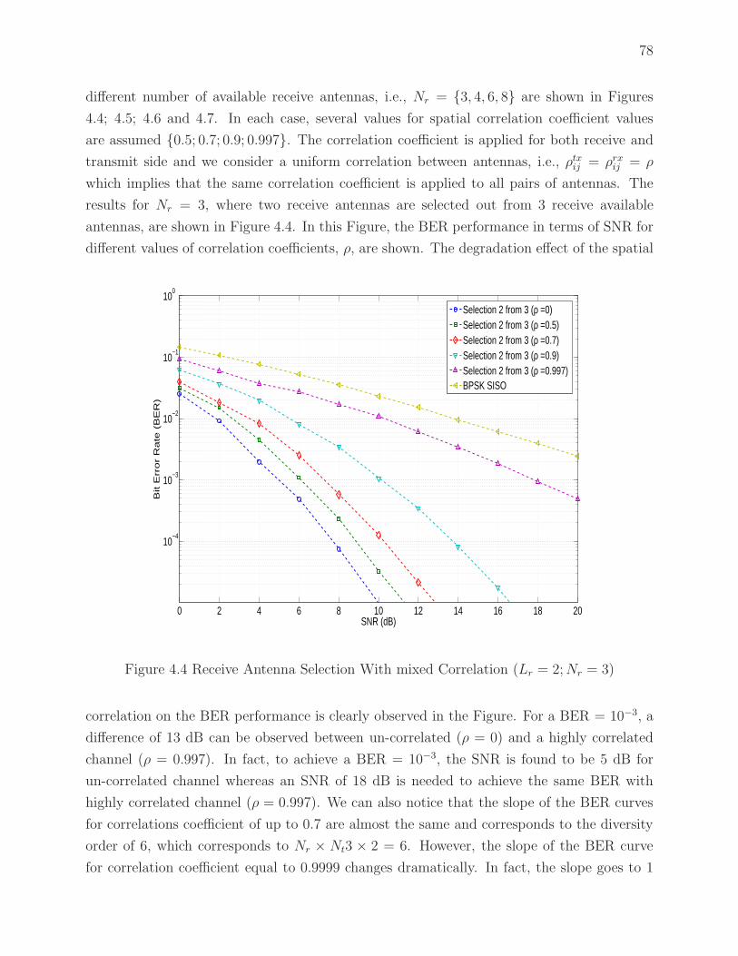
78

different number of available receive antennas, i.e., Nr = {3, 4, 6, 8} are shown in Figures

4.4; 4.5; 4.6 and 4.7. In each case, several values for spatial correlation coefficient values

are assumed {0.5; 0.7; 0.9; 0.997}. The correlation coefficient is applied for both receive and

transmit side and we consider a uniform correlation between antennas, i.e., ρtxij = ρrxij = ρ

which implies that the same correlation coefficient is applied to all pairs of antennas. The

results for Nr = 3, where two receive antennas are selected out from 3 receive available

antennas, are shown in Figure 4.4. In this Figure, the BER performance in terms of SNR for

different values of correlation coefficients, ρ, are shown. The degradation effect of the spatial

0 2 4 6 8 10 12 14 16 18 20

10−4

10−3

10−2

10−1

100

SNR (dB)

Bit E

rro

r R

ate

(B

ER

)

Selection 2 from 3 (ρ =0)Selection 2 from 3 (ρ =0.5)Selection 2 from 3 (ρ =0.7)Selection 2 from 3 (ρ =0.9)Selection 2 from 3 (ρ =0.997)BPSK SISO

Figure 4.4 Receive Antenna Selection With mixed Correlation (Lr = 2;Nr = 3)

correlation on the BER performance is clearly observed in the Figure. For a BER = 10−3, a

difference of 13 dB can be observed between un-correlated (ρ = 0) and a highly correlated

channel (ρ = 0.997). In fact, to achieve a BER = 10−3, the SNR is found to be 5 dB for

un-correlated channel whereas an SNR of 18 dB is needed to achieve the same BER with

highly correlated channel (ρ = 0.997). We can also notice that the slope of the BER curves

for correlations coefficient of up to 0.7 are almost the same and corresponds to the diversity

order of 6, which corresponds to Nr × Nt3 × 2 = 6. However, the slope of the BER curve

for correlation coefficient equal to 0.9999 changes dramatically. In fact, the slope goes to 1

79

for highly correlated channel (0.997), which is the same as the slope of the SISO curve. This

indicates that when the Rx antennas are fully correlated the diversity order of the system

will be equal to 1, which is the diversity order of SISO case. However, it can be observed

that in that case, the BER of the MIMO 2x2 system is still about 3 dB better compared to

SISO case (i.e. a gain). This is due to the fact that 2 antennas (even though they are fully

correlated) are in use and twice SNR (i.e., 3 dB) are received at the receiver side, compared

to SISO. Similar results about the BER for Nr = 4, 6 and 8 are shown in Figures 4.5, 4.6, 4.7.

In Figure 4.5, where Nr = 4, a difference of about 14 dB is observed between un-correlated

channel (ρ = 0) and highly correlated channel (ρ = 0.997) at a BER level equal to 10−3. In

fact, the SNR is found to be 4 dB for 10−3 BER, whereas an SNR of 18 dB is needed to

achieve the same level of BER (10−3).

0 2 4 6 8 10 12 14 16 18 20

10−4

10−3

10−2

10−1

100

SNR (dB)

Bit E

rro

r R

ate

(B

ER

)

Selection 2 from 4 (ρ =0)Selection 2 from 4 (ρ =0.5)Selection 2 from 4 (ρ =0.7)Selection 2 from 4 (ρ =0.9)Selection 2 from 4 (ρ =0.997)BPSK SISO

Figure 4.5 Receive Antenna Selection With mixed Correlation (Lr = 2;Nr = 4)

Again for correlation coefficients other than approximately equal to 1 (i.e. 0.5 and 0.7),

the slope of the curve corresponds to the diversity order of 8 (Nr × 2). This means that the

diversity order (Nr × Nt) is maintained for correlation coefficient not equal to 1. A similar

conclusion can be made when we consider Figures 4.6 and 4.7. Finally, to compare the

results of receive antenna selection with no selection, we plotted in Figure 4.8 presents the

80

0 2 4 6 8 10 12 14 16 18 20

10−4

10−3

10−2

10−1

100

SNR (dB)

Bit E

rro

r R

ate

(B

ER

)

Selection 2 from 6 (ρ = 0)Selection 2 from 6 (ρ = 0.5)Selection 2 from 6 (ρ = 0.7)Selection 2 from 6 (ρ = 0.9)Selection 2 from 6 (ρ = 0.997)BPSK SISO

Figure 4.6 Receive Antenna Selection With mixed Correlation (Lr = 2;Nr = 6)

BER curves for a fixed value of correlation coefficient and for different values of Nr as well

as the results of the 2× 2 Alamouti scheme without selection but with the same correlation

coefficient. The curve for 2×2 Alamouti without selection and zero correlation is also shown

in Figure 4.8. It can be seen from this Figure that for highly correlated channel increasing the

number of available antennas for receive antenna selection is also beneficial in terms of SNR

gain with respect to the BER performance. As can be seen increasing Nr reduces the average

BER and the performances becomes closer to the case of un-correlated 2×2 Alamouti scheme

since the best performance is obtained with 8 receive antennas available for selection. The

slopes of the curves tend to be different in the high SNR region, indicating that the diversity

order is increased by the number of available receive antennas Nr.

81

0 2 4 6 8 10 12 14 16 18 20

10−4

10−3

10−2

10−1

100

SNR (dB)

Bit E

rro

r R

ate

(B

ER

)

Selection 2 from 8 (ρ =0)Selection 2 from 8 (ρ =0.5)Selection 2 from 8 (ρ =0.7)Selection 2 from 8 (ρ =0.9)Selection 2 from 8 (ρ =0.997)BPSK SISO

Figure 4.7 Receive Antenna Selection With mixed Correlation (Lr = 2;Nr = 8)

82

0 2 4 6 8 10 12 14 16 18 20

10−4

10−3

10−2

10−1

100

SNR (dB)

Bit E

rro

r R

ate

(B

ER

)

2×2 Alamouti (No Selection; ρ = 0)Selection 2 From 3Selection 2 From 4Selection 2 From 6Selection 2 From 82×2 Alamouti (No Selection; ρ = 0.9)BPSK SISO

ρ = 0.9

2 × 2 Alamouti No Selection (ρ = 0)

Figure 4.8 BER of Receive Antenna Selection with mixed Correlation (ρ = 0.9)

83

CHAPTER 5

SUMMARY AND CONCLUSIONS

This dissertation consists of two main parts. The first part (Chapter 3) presents an

analysis and evaluation of the performance of MIMO-OFDM schemes in 4G LTE systems.

More specifically, we derive an average BER performance for two OSTBC diversity MIMO

schemes; namely the 2 × 1 SFBC-OFDM and the 4 × 2 FSTD-OFDM in the 3GPP 5 MHz

Long Term Evolution (LTE) system over a Rayleigh flat fading channel. To show the BER

performance improvement of the MIMO-OFDM schemes, the performance is compared to

the SISO configuration. To ascertain the accuracy of the analysis, we also performed Monte-

Carlo simulation using a LTE Link Level Simulator. The results show a good agreement

between numerical results and Monte-Carlo simulation results. To complete the analysis, a

study of the channel capacity for 2×1 SFBC-OFDM and 4×2 FSTD-OFDMMIMO schemes

in Rayleigh flat fading channel has been performed. We use the probability density function

of the instantaneous signal to noise ratio to derive analytical expressions for the capacity in

terms of exponential integral and Poisson distribution. Effective data throughput as mea-

sured through simulation compare well with the system channel capacity limit.

In the second part of this thesis (Chapter 4) we evaluated the performances of antenna

selection in MIMO systems. First, we reviewed antenna selection techniques and algorithms

in MIMO systems as well as OSTBC systems. We then presented a performance evaluation for

receive antenna selection in Rayleigh flat fading channels, assuming no antenna correlation.

We derived analytical expression for the BER performances using order statistics theory to

determine the probability density function of the signal to noise ratio of the selected subset of

antennas. The analytical results of the BER performance of OSTBC were expressed in terms

of an auxiliary integral. This integral can be evaluated using two known analytical defined

functions, namely, the incomplete gamma function and the Gauss hypergeometric function.

In our analysis, we considered a receive antenna selection where two receive antennas were

selected out of Nr available antennas. To verify the accuracy of our analysis, we performed

Monte-Carlo simulations and then compared the results to the theoretical analysis. For

Monte-Carlo simulations, we implemented the UCBS receive antenna selection algorithm.

The results show a good agreement between numerical values and Monte-Carlo simulations

results. The order statistics theory is restricted to non correlated channels and hence it

cannot be applied for correlated channels. Consequently we were constrained to evaluate the

84

performance of receive antenna selection in a correlated channels by Monte-Carlo simulations.

We used the Kronecker MIMO channel model to generate correlated MIMO channels. Using

the kronecker model, the antenna correlation at both sides are applied separately. Our results

showed that even in correlated channel, the receive antenna selection is beneficial compared

to no selection schemes.

5.1 Future Work

The performance analysis and evaluation presented in this thesis were made based on

some assumptions, like flat fading channel and uncorrelated channels. Future work, could

consider the following different assumptions.

5.1.1 MU-MIMO Aspects

In our performance evaluation of MIMO schemes in LTE (Chapter 3), we assumed a single

user MIMO system (SU-MIMO), where the same time frequency resources are allocated to

only one user. In addition to SU-MIMO as prescribed in the initial release of LTE standard,

different multi user MIMO schemes (MU-MIMO) have also been defined and hence can be

supported [44] by the standard. In MU-MIMO schemes, K UEs out of U active UEs in the

cell, where K is much smaller than U , are selected for simultaneous communication over the

same time frequency resource. For example, in a system with Nt transmit antennas and UEs

with single receive antenna each, Nt different users can be multiplexed, where each stream

is allocated to each UE. Thus, a substantial multiplexing gain can be achieved in case of

MU-MIMO with single antennas at the UEs. Another advantage of the MU-MIMO is the

natural de-correlation between the channels of the different UEs due to the fact that the

separation between the UEs is typically large relative to the wavelength. It then becomes

worthwhile to consider the performance of such systems.

5.1.2 CSI Aspects

One of the assumption which is consistently used throughout this work is perfect knowl-

edge of the channel state information at the receiver side. However in real implementation,

channel information is usually derived through channel estimation techniques which are not

always accurate. In LTE, the channel estimation is performed using the Reference Signals

(RS). As the signal in LTE evolves both in time and frequency domains, the channel esti-

mation can be performed in both domains, and the impact of each type of estimation on

the performance of LTE systems can be considered in the analysis. In the case of transmit

85

selection, which has not been considered in our work, the impact of the feedback delay should

also be considered in the analysis.

5.1.3 Frequency Selective Channel Aspects

In our performance evaluation in Chapter 4 of receive antenna selection , we used a flat

fading Rayleigh channel. In many situations the channel may be frequency selective. One

of the most important limitation of antenna selection occurs when the channel is frequency

selective. Indeed the different channel responses as a function of frequency imply that, in

each band, antenna selection should be different. Thus, whenever the channel is highly

frequency selective, antenna selection may not be useful or feasible. However, MIMO-OFDM

systems are known to view the frequency selective channel as N flat fading channels, where

N is the number of subcarriers in the OFDM symbol. In [35], the diversity order analysis

of antenna selection scheme over frequency selective channel has been considered while the

BER performance was evaluated by simulations only. Further studies of antenna selection in

such channels might be worthwhile of interest in the future.

5.1.4 Antenna Correlated Channel Aspects

In addition to the flat fading Rayleigh channel assumption in our performance analysis of

the receive antenna selection, we assumed uncorrelated channels in order to be able to apply

the theory of order statistics. In [57], an analysis of MIMO systems with receive antenna se-

lection in spatially correlated fading channels is provided using multivariate analysis together

with the Wishart distribution [23] but for the case of the selection of only one receive antenna.

Extensions to include more selections should be of great interest to investigate whether or

not the use of selection diversity is still of practical use in improving the performance.

5.1.5 Contributions and Publications

The results and analysis of the main work obtained in this thesis were published and

submitted in the following international conferences and journals:

1. BER Analysis of Alamouti Scheme with Receive Antenna Selection, published on 2010

6th International Conference of Wireless and Mobile Communications (ICWMC),

2. Investigation of the correlation effect on the Performance of V-BLAST and OSTBC

MIMO Schemes, published on the 2011 Seventh International Conference of Wireless

and Mobile Communicationss

86

3. Performance Evaluation of MIMO Schemes in 5 MHZ Bandwidth LTE Systems, pub-

lished on the 2012 8th International Conference of Wireless and Mobile Communications

4. Bit Error Analysis of MIMO Schemes in LTE Systems, published on the 2013 9th

International Conference of Wireless and Mobile Communications and received a best

paper award.

5. Analysis of the Performance for SFBC-OFDM and FSTD-OFDM Schemes in LTE Sys-

tems over MIMO Fading Channels, submitted to the International Journal On Advances

in Networks and Services as an Invited paper by IARIA Journals

6. Performance Analysis of MIMO Schemes in 3GPP Long Term Evolution System sub-

mitted to Springer’s Wireless Personal Communications

87

REFERENCES

[1] 3GPP (2009). Technical specification ts36.211 version 8.7.0 ”evolved universal

terresterial radio access (e-utra); physical channel and modulation, (release 8)”.

http://www.3gpp.org.

[2] 3GPP (2009). Technical specification ts36.212 ”evolved universal terresterial radio access

(e-utra); multiplexing and channel coding”. http://www.3gpp.org.

[3] 3GPP (2009). Technical specification ts36.213 ”evolved universal terresterial radio access

(e-utra); physical layer procedures”. http://www.3gpp.org.

[4] 3GPP (2013). Technical specification group radio access network.

http://www.3gpp.org.

[5] ALAMOUTI, S. (1998). A simple transmit diversity technique for wireless communica-

tions. Selected Areas in Communications, IEEE Journal on, 16, 1451 –1458.

[6] ALOUINI, M. S. and SIMON, M. K. (2000). Digital Communications over Fading

Channels: A Unified Approach to Performance Analysis, Wiley.

[7] ANDREWS, J. G. and GHOSH, A. (2007). Fundamentals of WiMAX: Understanding

Broadband Wireless Networking, PRENTICE HALL.

[8] ARNOLD, B. C., BALAKRISHNAN, N. and NAGARAJA, H. N. (1992). A first course

in order statistics. Wiley series in probability and mathematical statistics. J. Wiley, New

York. A Wiley-Interscience publication.

[9] BAHCECI, I., DUMAN, T. and ALTUNBASAK, Y. (2003). Antenna selection for

multiple-antenna transmission systems: performance analysis and code construction.

Information Theory, IEEE Transactions on, 49, 2669–2681.

[10] CHOI, Y.-S., MOLISCH, A., WIN, M. and WINTERS, J. (2003). Fast algorithms for

antenna selection in mimo systems. Vehicular Technology Conference, 2003. VTC 2003-

Fall. 2003 IEEE 58th. vol. 3, 1733–1737 Vol.3.

[11] DAVID, H. (1981). Order statistics. Wiley series in probability and mathematical

statistics. Applied probability and statistics. Wiley.

[12] ESPINOSA, H. C., FONOLLOSA, J. R. and PENIN, J. A. D. (2001). Channel capacity

of space-time block coding. in Proc. IST Mobile Communications. 9–14.

[13] GHRAYEB, A. (2006). A survey on antenna selection for mimo communication systems.

Information and Communication Technologies, 2006. ICTTA ’06. 2nd. vol. 2, 2104–2109.

88

[14] GIFFORD, W. M., WIN, M. Z. and CHIANI, M. (2008). Antenna subset diversity

with non-ideal channel estimation. IEEE Transactions on Wireless Communications, 7,

1527–1539.

[15] GOLDEN, G., FOSCHINI, C. J., VALENZUELA, R. and WOLNIANSKY, P. (1999).

Detection algorithm and initial laboratory results using v-blast space-time communica-

tion architecture. Electronics Letters, 35, 14–16.

[16] GOLDSMITH, A. (2005). Wireless Communications. Cambridge University Press, New

York, NY, USA.

[17] GORE, D., NABAR, R. and PAULRAJ, A. (2000). Selecting an optimal set of transmit

antennas for a low rank matrix channel. Acoustics, Speech, and Signal Processing, 2000.

ICASSP ’00. Proceedings. 2000 IEEE International Conference on. vol. 5, 2785–2788

vol.5.

[18] GORE, D. and PAULRAJ, A. (2002). Mimo antenna subset selection with space-time

coding. Signal Processing, IEEE Transactions on, 50, 2580–2588.

[19] GOROKHOV, A. (2002). Antenna selection algorithms for mea transmission systems.

Acoustics, Speech, and Signal Processing (ICASSP), 2002 IEEE International Confer-

ence on. vol. 3, III–2857–III–2860.

[20] GRADSHTEYN, I. S. and RYZHIK, I. M. (1994). Table of Integrals, Series and

Products. Academic Press, San Diego, cinquieme edition. Erratum available from

www.mathtable.com.

[21] GRADSHTEYN, I. S. and RYZHIK, I. M. (2000). Table of Integrals, Series and

Products. Academic Press, San Diego, sixth edition. Erratum available from

www.mathtable.com.

[22] GUNTHER, C. (1996). Comment on ”estimate of channel capacity in rayleigh fading

environment. Vehicular Technology, IEEE Transactions on, 45, 401–403.

[23] HAGEDORN, M., SMITH, P., BONES, P., MILLANE, R. and PAIRMAN, D. (2006). A

trivariate chi-squared distribution derived from the complex wishart distribution. Jour-

nal of Multivariate Analysis, 97, 655 – 674.

[24] HEATH, R. and PAULRAJ, A. (2001). Antenna selection for spatial multiplexing sys-

tems based on minimum error rate. Communications, 2001. ICC 2001. IEEE Interna-

tional Conference on. vol. 7, 2276–2280 vol.7.

[25] IKUNO, J., WRULICH, M. and RUPP, M. (2010). System level simulation of lte net-

works. Vehicular Technology Conference (VTC 2010-Spring), 2010 IEEE 71st. 1 –5.

[26] JOHNSON, C. (2012). Long Term Evolution IN BULLETS, PRENTICE HALL. Sec-

onde edition.

89

[27] KATZ, M., TIIROLA, E. and YLITALO, J. (2001). Combining space-time block coding

with diversity antenna selection for improved downlink performance. Vehicular Tech-

nology Conference, 2001. VTC 2001 Fall. IEEE VTS 54th. vol. 1, 178–182 vol.1.

[28] KERMOAL, J., SCHUMACHER, L., PEDERSEN, K., MOGENSEN, P. and FRED-

ERIKSEN, F. (2002). A stochastic mimo radio channel model with experimental vali-

dation. Selected Areas in Communications, IEEE Journal on, 20, 1211–1226.

[29] LEGNAIN, R., HAFEZ, R. H. M. and MARSLAND, I. (2012). Ber analysis of three-

phase xor-and-forward relaying using alamouti stbc. Communications Letters, IEEE,

16, 1458–1461.

[30] LOPEZ-MARTINEZ, F., MARTOS-NAYA, E., WONG, K.-K. and ENTRAM-

BASAGUAS, J. (2011). Closed-form ber analysis of alamouti-mrc systems with icsi

in ricean fading channels. Communications Letters, IEEE, 15, 46–48.

[31] MAAREF, A. and AISSA, S. (2005). Capacity of space-time block codes in mimo

rayleigh fading channels with adaptive transmission and estimation errors. Wireless

Communications, IEEE Transactions on, 4, 2568–2578.

[32] MEHLFUHRER, C., WRULICH, M., IKUNO, J. C., BOSANSKA, D. and RUPP, M.

(2009). Simulating the long term evolution physical layer. Proc. of the 17th European

Signal Processing Conference (EUSIPCO 2009). Glasgow, Scotland.

[33] MOLISCH, A. (2004). Mimo systems with antenna selection - an overview. Mitsubishi

Electric Research Labs. 1–22.

[34] MOLISCH, A., WIN, M. and WINTERS, J. (2001). Capacity of mimo systems with

antenna selection. Communications, 2001. ICC 2001. IEEE International Conference

on. vol. 2, 570–574 vol.2.

[35] OHNO, S. and TEO, K. (2009). Diversity analysis of antenna selection over frequency-

selective mimo channels. Acoustics, Speech and Signal Processing, 2009. ICASSP 2009.

IEEE International Conference on. 2813–2816.

[36] ONLINE (2009). Lte link level simulator. Available

http://www.nt.tuwien.ac.at/ltesimulator.

[37] PARK, J.-S. and PARK, D.-J. (2005). A new antenna selection algorithm with low

complexity for mimo wireless systems. Communications, 2005. ICC 2005. 2005 IEEE

International Conference on. vol. 4, 2308–2312 Vol. 4.

[38] PRASSARD, R. (2001). OFDM for Wireless Communications Systems. Artech House.

[39] PROAKIS, J. G. (2001). Digital Communications, Mc Graw Hill.

90

[40] SANDHU, S. and PAULRAJ, A. (2000). Space-time block codes: a capacity perspective.

Communications Letters, IEEE, 4, 384–386.

[41] SCHWARZ, S., MEHLFUHRER, C. and RUPP, M. (2010). Calculation of the spatial

preprocessing and link adaption feedback for 3gpp umts/lte. Wireless Advanced (WiAD),

2010 6th Conference on. 1 –6.

[42] SCHWARZ, S., WRULICH, M. and RUPP, M. (2010). Mutual information based cal-

culation of the precoding matrix indicator for 3gpp umts/lte. Smart Antennas (WSA),

2010 International ITG Workshop on. 52 –58.

[43] SESIA, S., ISSAM, T. and BACKER, M. (2011). LTE The UMTS Long Term Evolution

From Theory To Practice, John Wiley.

[44] SESSIA, S., TAOUFIK, I. and BAKER, M. (2011). LTE The UMTS Long Term Evo-

lution: From THEORY TO PRACTICE, WILEY. Seconde edition.

[45] SHANNON, C. E. (1948). A mathematical theory of communication. The Bell System

Technical Journal, 27, 379–423, 623–656.

[46] SHEN, H. and GHRAYEB, A. (2006). Analysis of the outage probability for mimo

systems with receive antenna selection. Vehicular Technology, IEEE Transactions on,

55, 1435–1440.

[47] SIMKO, M., MEHLFUHRER, C., WRULICH, M. and RUPP, M. (2010). Doubly dis-

persive channel estimation with scalable complexity. Smart Antennas (WSA), 2010

International ITG Workshop on. 251 –256.

[48] SIMON, M. K. and ALOUINI, M.-S. (1998). A unified approach to the performance

analysis of digital communication over generalized fading channels. Proceedings of the

IEEE, 86, 1860–1877.

[49] TAROKH, V., JAFARKHANI, H. and CALDERBANK, A. (1999). Space-time block

codes from orthogonal designs. Information Theory, IEEE Transactions on, 45, 1456–

1467.

[50] TAROKH, V., JAFARKHANI, H. and CALDERBANK, A. (1999). Space-time block

codes from orthogonal designs. Information Theory, IEEE Transactions on, 45, 1456–

1467.

[51] TELATAR, I. E. (1999). Capacity of multi-antenna gaussian channels. EUROPEAN

TRANSACTIONS ON TELECOMMUNICATIONS, 10, 585–595.

[52] TORABI, M. and HACCOUN, D. (2011). Performance analysis of joint user scheduling

and antenna selection over mimo fading channels. Signal Processing Letters, IEEE, 18,

235–238.

91

[53] TSE, D. and VISWANATH, P. (2008). Fundamnetals of Wireless Communications,

Cambridge University Press.

[54] WONG, W. H. and LARSSON, E. (2003). Orthogonal space-time block coding with

antenna selection and power allocation. Electronics Letters, 39, 379–381.

[55] WRULICH, M. (2006). Capacity Analysis of MIMO Systems. Memoire de maıtrise,

Institut fur Nachrichtentechnik und Hochfrequenztechnik, Vienna University of Tech-

nology.

[56] XIE, W., XIE, L., ZHAN, J. and LIU, S. (2006). A novel antenna selection algorithm

for mimo systems under correlated channels. ITS Telecommunications Proceedings, 2006

6th International Conference on. 461–464.

[57] XU, Z., SFAR, S. and BLUM, R. (2009). Analysis of mimo systems with receive antenna

selection in spatially correlated rayleigh fading channels. Vehicular Technology, IEEE

Transactions on, 58, 251–262.

[58] ZENG, X. N. and GHRAYEB, A. (2004). Performance bounds for space-time block

codes with receive antenna selection. Information Theory, IEEE Transactions on, 50,

2130–2137.

[59] ZHANG, H. and GULLIVER, T. (2005). Capacity and error probability analysis for

orthogonal space-time block codes over fading channels. Wireless Communications,

IEEE Transactions on, 4, 808–819.

92

APPENDICE A

IMPACT OF RECEIVE ANTENNA CORRELATION

To evaluate the impact of only receive antenna correlation, we performed different sim-

ulation when the antenna correlation at the transmitter is equal to 0 (i.e., the transmit

correlation matrix is the identity matrix, Rtx = I) and only receive antenna correlation is

considered. The results for the 2× 2 scheme without receive antenna selection and for differ-

ent values of correlation coefficient (ρrx = {0.5, 0.7, 0.9, 0.99999}) are shown in Figure A.1.

In this Figure, the BPSK BER performances of the 2 × 2 Alamouti scheme are shown. It

0 2 4 6 8 10 12 14 16 18 20

10−4

10−3

10−2

10−1

100

SNR (dB)

Bit E

rro

r R

ate

(B

ER

)

No Selection 2 × 2 (ρrx

= 0)

No Selection 2 × 2 (ρrx

= 0.5)

No Selection 2 × 2 (ρrx

= 0.7)

No Selection 2 × 2 (ρrx

= 0.9)

No Selection 2 × 2 (ρrx

= 0.99999)

Alamouti 2x1 BPSK SISO

Figure A.1 BER of Receive Antenna Selection with receive antenna Correlation (ρtx = 0)

can be noticed from the Figure that the recieve antenna correlation deteriorate the BER

performances. When the correlation coefficient tends to 1 (ρrx = 0.99999), the slope of the

BER curve becomes equal to 2. In fact, it is clearly shown in the Figure that the curve

of 2 × 2 scheme with highly receive antenna correlation (ρrx = 0.99999) is almost parallel

93

to the curve of the 2 × 1 scheme without any correlation. Also, it can be noticed that the

curve of the 2 × 2 scheme is just shifted by almost 3 dB with respect to the 2 × 1 scheme,

which represents a 3 dB SNR gain with respect to the 2 × 1 case. This 3 dB improvement

with respect to the 2 × 1 case is explained by the fact that the two receive antennas act as

one receive antenna with a double SNR when the correlation coefficient is almost equal to 1.

The results for Nr = 3, 4, 6, and 8 are shown in Figures A.2, A.3, A.4 and A.5, respectively.

In those Figures, we plotted the BPSK BER performance of 2 × 2 Alamouti scheme with

receive antenna selection in correlated channel and where the correlation coefficients values

are the same as before. The results when two receive antennas are selected out of three

receive available antennas are shown in Figure A.2. We can notice from the Figure that the

0 2 4 6 8 10 12 14 16 18 20

10−4

10−3

10−2

10−1

100

SNR (dB)

Bit E

rro

r R

ate

(B

ER

)

Selection 2 / 3 (ρrx

= 0)

Selection 2 / 3 (ρrx

= 0.5)

Selection 2 / 3 (ρrx

= 0.7)

Selection 2 / 3 (ρrx

= 0.9)

Selection 2 / 3 (ρrx

= 0.99999)

Alamouti 2x1 BPSK SISO

Figure A.2 BER of Receive Antenna Selection with receive antenna Correlation (ρtx = 0 andNr = 3)

receive antenna correlation deteriorates the BER performance. In fact, in case of uncorre-

lated receive antennas (ρrx = 0), the BER level of 10−3 is achieved with SNR value equal to

5 dB, whereas the same BER level is achieved with 11 dB when the correlation coefficient

is almost equal to 1 (ρrx = 0.99999), which represents a degradation of 6 dB. It can also be

observed from the Figure how the slope of the curve tends to be the same as the 2×1 case as

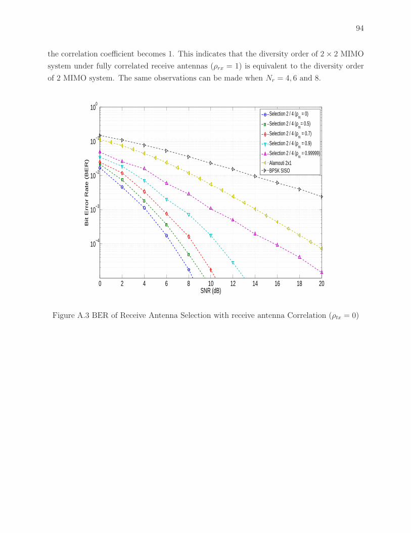
94

the correlation coefficient becomes 1. This indicates that the diversity order of 2× 2 MIMO

system under fully correlated receive antennas (ρrx = 1) is equivalent to the diversity order

of 2 MIMO system. The same observations can be made when Nr = 4, 6 and 8.

0 2 4 6 8 10 12 14 16 18 20

10−4

10−3

10−2

10−1

100

SNR (dB)

Bit E

rro

r R

ate

(B

ER

)

Selection 2 / 4 (ρrx

= 0)

Selection 2 / 4 (ρrx

= 0.5)

Selection 2 / 4 (ρrx

= 0.7)

Selection 2 / 4 (ρrx

= 0.9)

Selection 2 / 4 (ρrx

= 0.99999)

Alamouti 2x1 BPSK SISO

Figure A.3 BER of Receive Antenna Selection with receive antenna Correlation (ρtx = 0)

95

0 2 4 6 8 10 12 14 16 18 20

10−4

10−3

10−2

10−1

100

SNR (dB)

Bit E

rro

r R

ate

(B

ER

)

Selection 2 / 6 (ρrx

= 0)

Selection 2 / 6 (ρrx

= 0.5)

Selection 2 / 6 (ρrx

= 0.7)

Selection 2 / 6 (ρrx

= 0.9)

Selection 2 / 6 (ρrx

= 0.99999)

Alamouti 2x1 BPSK SISO

Figure A.4 BER of Receive Antenna Selection with receive antenna Correlation (ρtx = 0)

96

0 2 4 6 8 10 12 14 16 18 20

10−4

10−3

10−2

10−1

100

SNR (dB)

Bit E

rro

r R

ate

(B

ER

)

Selection 2 / 8 (ρrx

= 0)

Selection 2 / 8 (ρrx

= 0.5)

Selection 2 / 8 (ρrx

= 0.7)

Selection 2 / 8 (ρrx

= 0.9)

Selection 2 / 8 (ρrx

= 0.99999)

Alamouti 2x1BPSK SISO

Figure A.5 BER of Receive Antenna Selection with receive antenna Correlation (ρtx = 0)

97

APPENDICE B

DERIVATION OF THE ALTERNATIVE FORM OF Q-FUNCTION

The classical expression of the Q-function is defined by:

Q(x) =

∫ ∞

x

1√2π

exp

(−y2

2

)dy (B.1)

.

The following derivation is aimed to obtain an alternative form of Equation (B.1), where

the lower limit of the integral is independent of the variable x and the upper limit is finite.

To this end, the starting point of the derivation is to consider the integral due to [20] [p. 362,

Eq. (3.363.2)]

∫ ∞

u

e−µx

x√x− u

dx =π√uerfc (

√uµ) (B.2)

.

Putting u = y2 and multiplying both sides of Equation (B.2) by 12eµu gives

1

2

∫ ∞

y2

e−µx

x√x− u

dx =π

2yeµy

2

erfc (yõ) (B.3)

.

In order to extend the Equation (B.3) to two dimension (x, y), we define u = x− y2. The

Equation (B.3) then becomes:

1

2

∫ ∞

0

e−µu

(u+ y2)√udu =

π

2yeµy

2

erfc (yõ) (B.4)

.

Now, we define u = t2, which leads to du = 2tdt = 2√udt. Hence, Equation (B.4) be-

comes:

98

∫ ∞

0

e−µt2

(t2 + y2)dt =

π

2yeµy

2

erfc (yõ) (B.5)

.

Putting y = 1 andµ = z2 in the above equation, we obtain:

∫ ∞

0

e−z2t2

(t2 + 1)dt =

π

2ez

2

erfc (z) (B.6)

.

Equivalently, Equation (B.6) can be written as:

2

π

∫ ∞

0

e−z2(t2+1)

(t2 + 1)dt = erfc (z) (B.7)

.

The final step in the derivation of the alternative form of the Q- function is to let

sin2θ = (t2 + 1)−1 and cos2θ = t2(t2 + 1), which leads to a derivation of t with respect

to θ as:

dt = −(t2 + 1)dθ (B.8)

and the Equation (B.7) becomes:

2

π

∫ π2

0

exp

( −z2

sin2θ

)dθ = erfc (z) (B.9)

by letting z = x√2, we finally obtain the desired alternative form of the Q-function as:

1

π

∫ π2

0

exp

(− x2

2 sin2θ

)dθ = Q(x) (B.10)

99

which conclude the derivation of the alternative form of the Q-function.

It is worth noting that there is another different method to arrive to the form of Equation

(B.10), which can be found in [6].

100

APPENDICE C

BER EVALUATION USING THE ALTERNATIVE Q-FUNCTION

To compute the average error probability, an integral whose integrand consists of the

product of the Gaussian Q-function and the probability density function (PDF) of the fading

channel have to be evaluated. If one has to use the classical form of the Q-function, the

integral for the evaluation will have the following form:

I =

∫ ∞

0

Q(a√γ)pγ(γ)dγ =

∫ ∞

0

[∫ ∞

a√γ

1√2π

exp

(−y2

2

)dy

]pγ(γ)dγ (C.1)

where γ represents the average signal to noise ratio and a is constant that depends on the spe-

cific modulation scheme. As discussed, in general, the evaluation of the integral in Equation

(C.1) is difficult because of the presence of√γ in the lower limit of the integral. However,

if, instead, the alternative form of the Q-function (Appendix A; Equation (B.10)) has to be

used, the evaluated integral becomes:

I =

∫ ∞

0

[1

π

∫ π/2

0

exp

(− a2γ

2 sin2θ

)dθ

]pγ(γ)dγ (C.2)

or equivalently

I =1

π

∫ π/2

0

[∫ ∞

0

exp

(− a2γ

2 sin2θ

)pγ(γ)dγ

]dθ (C.3)

where the integral in brackets (inner integral) is i the form of a Laplace transform with respect

to the variable γ. In fact, the Laplace transform of pγ(γ) represents the Moment Generating

Function of γ, which is defined by:

Mγ(s) =

∫ ∞

0

esγpγ(γ)dγ (C.4)

and hence Equation (C.3) can be written as:

I =1

π

∫ π/2

0

Mγ

(− a2

2 sin2θ

)dθ (C.5)

.

Using the above integral, the evaluation of the error probability is simplified to the eval-

101

uation a single integral on θ. The first step in the evaluation is then the calculation of the

Laplace transform of the probability density function (PDF) of the instantaneous SNR, which

represents the Moment Generating Function (MGF) of γ. The second step consists of the

evaluation of a single integral on θ.

102

APPENDICE D

VIENNA LTE LINK LEVEL SIMULATOR

In order to verify the analysis of LTE performances with Monte-Carlo simulation, a full

LTE transmission chain have to be implemented to perform those simulations. However,

LTE is a complex system and implementing all the functionalities and features of this system

would require a huge time. Fortunately, an LTE link level simulator has been made publicly

under an academic use license including source code by Vienna Technical University. This

enabled academic researches access to an open source LTE simulator, which facilitates the

comparison and sharing different algorithm and results. In this thesis, we used the Vienna

LTE link level simulation to verify our analysis and perform some evaluations of LTE sys-

tem performances. The simulator is a software implementation of the physical (PHY) layer

procedures. The Link Level Simulator is aimed to simulate one or multiple links between the

Evolved base station (eNodeB) and the User Equipment (UE), including channel model. In

this appendix, we provide a brief description of the overall structure of the simulator used in

this thesis.

The Vienna link level simulator consists of three main blocks, namely Transmitter (TX),

Channel Model and Receiver (RX) as shown in Figure D.1.

Figure D.1 Functional Block Diagram of Vienna LTE Link Level Simulator

The signaling, from transmitter to the receiver, and the User Equipment feedback, from

the receiver to the transmitter and expressed in terms of Channel State Information (CSI)

103

and acknowledjement/non acknowledgement (ACK/NACK), are assumed to be error free

and that is why they are not connected to the channel model.

The functional block diagram of the transmitter is shown in Figure D.1 and represents the

implementation of the transmission procedures as described in the corresponding technical

specification series (TS). Specifically, the physical layer of LTE are described in TS 36.x series

[2], [1], [3].

Figure D.2 Functional Block Diagram of the Transmitter of the LTE Simulator

Based on the feedback values received from the UE, the scheduling algorithm in the trans-

mitter assigns each UE specific Resource Blocks (RBs), a modulation and coding scheme

(MCS), an MIMO transmission mode and an appropriate pre-coding matrix for spatial mul-

104

tiplexing. The transmitted signal can be modulated using 4-QAM, 16-QAM or 64-QAM

modulations alphabets with discrete set of coding rates as specified in. Three main MIMO

modes can be supported by the simulator, namely Transmit Diversity (TxD); Open loop spa-

tial multiplexing (OLSM) and Closed Loop Spatial Multiplexing (CLSM). For each MIMO

mode, different antennas configuration can be supported. For example, in TxD mode tho

possibilities of antennas configuration can be supported, namely 2× 1 and 4× 2, where 2× 1

means two transmit antennas and one receive antennas.

Two types of fading channels can be supported by the Vienna LTE simulator, namely

block fading channels and fast fading channels. In the case of block fading channel, the

channel coefficient is constant during the duration of one sub-frame (1 ms). In fast fading

channels, time correlated channel impulse response are generated for each sample of the

transmitted signal. The channel models that can be supported by the LTE simulator are as

follow:

1. Additive White Gaussian Noise (AWGN)

2. Rayleigh Flat Fading Channel

3. Channel models based on the Power Delay Profile (PDP) such as ITU Pedestrian B

and ITU Vehicular A channel models.

4. Winner Phase II channel model

The receiver in the LTE simulator is implemented with many options in terms of receiver

algorithm, channel estimation and feed back calculations. The overall structure of the im-

plemented receiver in LTE is shown in Figure D.3. As detection algorithms, the receiver

can support Zeros Forcing (ZF), Linear Minimum Mean Square Error (LMMSE) and Soft

Sphere Decoding (SSD) algorithms. In terms of channel estimation, four different types of

channel estimator are implemented, namely Least Square (LS), Minimum Mean Square Error

(MMSE), approximate Linear Minimum Mean Square Error (LMMSE) and perfect channel

knowledge based on all transmitted symbols. The feedback information to be sent to the

transmitter are calculated based on the results of channel estimation. The feedback infor-

mation include the Channel Quality Indicator (CQI) for all modes of operation, the Rank

Indicator (RI) for spatial multiplexing modes and finally the Pre-coding Matrix Indicator

(PMI) for Closed Loop Spatial Multiplexing Mode (CLSM). The structure of the receiver

allows the investigation of various aspects, such as channel estimation, frequency and time

synchronisation algorithms, modeling of the channel encoding and decoding and physical

layer modeling for system level simulation.

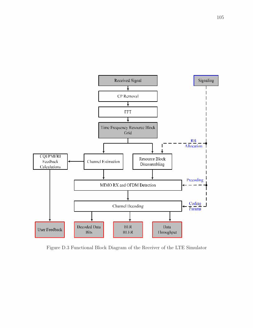
105

Figure D.3 Functional Block Diagram of the Receiver of the LTE Simulator