performance evaluation of aodv routing protocol:...
TRANSCRIPT

Performance Evaluation of AODV Routing Protocol: Real-Life Measurements
Semester Project Report
Project Supervisors:
Mario Čagalj LCA, EPFL
Prof. Jean-Pierre Hubaux
LCA, EPFL
Alexander Zurkinden, SCC June, 2003

2
Table of Contents
1. Introduction ................................................................................ 3
2. Mobile Ad-Hoc Networks........................................................... 3
2.1 Overview......................................................................................................................... 3
2.1 Terminology.................................................................................................................... 5
2.2 Characteristics................................................................................................................ 5
2.3 Routing in MANET ........................................................................................................ 5 2.3.1 Proactive Protocol..................................................................................................................... 6 2.3.2 Reactive Protocol...................................................................................................................... 6
3. IEEE 802.11................................................................................. 6
4. AODV .......................................................................................... 7
4.1 Overview......................................................................................................................... 7
4.2 Route Discovery.............................................................................................................. 8
4.3 Route Maintenance......................................................................................................... 8
4.4 Hello Messages................................................................................................................ 9
5. Experimental Setup .................................................................... 9
5.1 System components .......................................................................................................10
5.2 Software Tools ...............................................................................................................11 5.2.1 AODV-UU ............................................................................................................................. 11 5.2.2 AODV-UCSB......................................................................................................................... 11 5.2.3 PING...................................................................................................................................... 11 5.2.4 NetPIPE.................................................................................................................................. 11 5.2.5 MGEN.................................................................................................................................... 12 5.2.6 Iptables................................................................................................................................... 12
5.3 Set-up of the mobile Ad-Hoc network experiments......................................................12 5.3.1 Set-up of the real multihop experiments....................................................................................... 13 5.3.2 Set-up for the forced multihop experiments .................................................................................. 13 5.3.3 Mobility experiment set-up .......................................................................................................... 15
6. Results and Comments ............................................................. 15
6.1 Route Discovery Time ...................................................................................................16
6.2 Packet Loss Performance ..............................................................................................18
6.3 End-to-End Delay Performance....................................................................................19
6.4 Throughput using TCP traffic ......................................................................................22
6.5 Throughput using UDP traffic ......................................................................................28
6.6 Mobility..........................................................................................................................30
7. Conclusion................................................................................. 34
8. Bibliography.............................................................................. 36

3
1. Introduction
Mobile Ad- Hoc networking has gained an important part of the interest of researchers and become very popular this past few years, due to its potential and possibilities. With a MANET computing is not restrained on locality, time nor on mobility. Computing therefore can be done anywhere and anytime!
IEEE 802.11 which are the official standards for wireless communication take only single-hop networks into account. Therefore routing protocols, for network without infrastructures, have to be developed. These protocols determine how messages can be forwarded, from a source node to a destination node which is out of the range of the former, using other mobile nodes of the network. Routing, which includes for example maintenance and discovery of routes, is one of the very challenging areas in communication. Many protocols have been proposed [1] – [3] under which AODV [4] (Ad-Hoc On-demand Distance Vector).
Numerous simulations of routing protocols have been made using different simulators, such as ns and GloMoSim. Simulators though cannot take into account of all the factors that can come up in real life and performance and connectivity of mobile Ad-Hoc network depend and are limited also by such factors. Routing algorithms are being developed for commercial purposes and thus will be used outside of laboratories and simulators. There was our motivation to evaluate the behavior of a routing protocol in real-life scenarios which can come up in everyday life. As routing protocol AODV has been chosen, since in our opinion the ideas behind it are very promising.
Specifically we decided to perform real life experiments and comparisons using the two implementations of AODV developed at the University of California in Santa Barbara (UCSB), USA and the Uppsala University (UU), Sweden. The impact of varying packet size, route length and mobility in Ad- Hoc networks on connectivity, packet loss, Route Discovery Time and throughput was tested.
In possible real life experiences, where each node has exactly one up- and one downstream neighbor, distance get with increasing number of hops fast extremely long. This can lead, when doing experiments with many nodes, to problems. There was our second motivation to discover if there is another possibility than using simulators, to evaluate networks and how well this would reflect results obtained in a similar real life set-up. Advantage was taken of the possibility of dropping messages at a node from other specified nodes. That way the real life set-up was moved into a room where distances are short.
In this paper we first give an introduction to Ad-Hoc Mobile Networks and different routing methods. Chapter 3 presents a summary of IEEE 802.11. In chapter 4 AODV and its characteristics are discussed. The set-up of the experiments and the used software are described in chapter 5. The obtained results are presented in chapter 6. Finally in chapter 7 we come to the conclusion of this project.
2. Mobile Ad-Hoc Networks 2.1 Overview
Mobile Ad-Hoc Network (MANET) is a recent developed part of wireless communication. The difference to traditional wireless networks is that there is no need for established infrastructure. Since there is no such infrastructure and therefore no preinstalled routers which can, for example, forward packets from one host to another, this task has to be

4
taken over by participants, also called mobile nodes, of the network. Each of those nodes take equal roles, what means that all of them can operate as a host and as a router.
Next to the problems of traditional wireless networks such as security, power control, transmission quality and bandwidth optimization, new problems come up in Ad-Hoc networks. We have in mind problems like maintenance and discovery of routes and topological changes of the network. To solve such problems is the challenge of Ad-Hoc Networking.
In figures 2.1.1. are examples of a infrastructure, a wireless and a Ad-Hoc network presented.
Fig. 2.1.1.i Example of a LAN
Fig. 2.1.1.ii Example of a WLAN
Fig. 2.1.1.iii Example of a Ad-Hoc network

5
2.1 Terminology
• Packet – A unit of data. A message is made out of several packets • Transmission Range – The area in which the signal of a sending node can be
received • Node – Participant of the network such as a laptop computer or a mobile phone • Source Node – Node that wants to send a message • Destination Node – Node which is the intended receiver of the message • Intermediate Node – All the nodes of a route which forward packets • Route – Path made out of different nodes to connect the source to the destination
node • Hop – The number of hops of a route is one smaller than the number of its containing
nodes • Flooding – The easiest way of routing. A message is send to all the machines and
forwarded from those machines until the destination of the messages is reached • Unicast – A message is send from one sender to exactly one receiver • Multicast – A message is send from one sender to multiple receivers with a single
send operation • Local Broadcast – A message is send to all the nodes within the transmission range
2.2 Characteristics
• Nodes – All the nodes in a mobile Ad-Hoc network, regardless of their position, can communicate with other nodes with the same priority. Since there is no infrastructure there is a need, in order to let distant nodes communicate with each other, of nodes in the network who take over the position of a router.
• Loss rate and delay – The communication medium of wireless networks, electromagnetic waves, encounter during their propagation many interference coming from objects which are in the propagation way of the waves or from other transmitting wireless devices. Therefore we have in MANETs a higher loss rate and delay than in wired networks.
• Topology – Since the nodes in an Ad-Hoc network are mobile the chance of frequent changes in the topology of the network is high. Algorithms for Ad-Hoc networks have to take these topological changes into account.
• Security – Because the computer communicate over the air, every node, equipped with the necessary utilities, inside the transmitting area of a sending node, can receive the sent messages. For this reason wireless network are less secure than wired ones.
• Capacity – At the moment is the amount of data which a link of a wireless network is able to transmit per unit of time smaller than the one of a wired network.
2.3 Routing in MANET
Routing in a MANET is done with the goal of finding a short and optimized route from the source to the destination node. In this section we describe briefly ways in which such a route can be determined. Next to the two described protocols there exist also Hybrid protocols, which are a combination of the other two.

6
2.3.1 Proactive Protocol
One possible routing protocol is a proactive protocol. The idea of such a protocol is to keep track of routes from a source to all destination in the network. That way as soon as a route to a destination is needed it can be selected in the routing table. Advantages of a proactive protocol are that communication experiences a minimal delay and routes are kept up to date. Disadvantages are the additional control traffic and that routes may break, as a result of mobility, before they are actually used or even that they will never be used at all, since no communication may be needed from a specific source to a destination.
An example of a proactive protocol is the Destination Sequence Distance Vector (DSDV) protocol [2]. In the DSDV algorithm each node keeps track of routing information, like number of hops to destination, sequence number of destination and the next hop on the route to the destination. The sequence number is provided by the destination host itself, to assure loop freedom. This means that the routes for a destination never form a cycle. Since topology may vary frequently, each node transmits periodically updates, including the nodes accessible from it and the length of the route to this node. When an other node receives such a update it compares the update with its own routing table and keeps the information with the highest sequence number. If the information in the update and those of its routing table have the same sequence number for a node, the entry with the shortest route is kept. 2.3.2 Reactive Protocol
Another way of routing in a MANET are reactive protocols or also called on demand protocols. They use the concept of acquiring information about routing only when needed. An advantage is that smaller bandwidth is needed for maintaining routing tables. A disadvantage is that when a route is needed we encounter a non negligible delay, since before using the route for a specific communication, it has to be determined.
An example of a reactive protocol is the Dynamic Source Routing (DSR) protocol [3]. It is based on the two mechanisms of Route Discovery and Route Maintenance used to discover and maintain information about routes. Those two mechanisms are operated on demand.
When a route is needed and it is not already known by a node it sends a Route Request (RREQ) message to its neighbors. Those forward the message until it reaches the destination node. Each intermediate node updates the RREQ with its address. When a node sends a RREQ message it attaches to it a request ID. The request ID and the IP address of the node form a unique identifier. This is done in order to prevent that an intermediate node which receives twice the same RREQ message forwards it twice.
When the destination receives the RREQ it sends a Route Reply (RREP) message back to the source node by reversing the hop sequence recorded in the RREQ. When the source receives the RREP it can start communicating with the destination, by including the whole route in the header of each to be sent message.
3. IEEE 802.11
The scope of IEEE 802.11 [5] is to develop and maintain specifications for wireless connectivity for fixed, portable and moving stations within a local area. It defines over-the-air protocols necessary to support networking in a local area. This standard provides MAC and physical layer functionality. The extension 802.11b (the MAC protocol used in our studies) gives accommodation of transmission rates of up to 11 Mbps and operates in the 2.4 GHz band. The 802.11 standard takes into account of power management, bandwidth, security and addressing, since these are the significant differences from wireless to wired LANs. The
7
MAC layer of the 802.11 standard provides access control functions, such as addressing, access coordination etc.
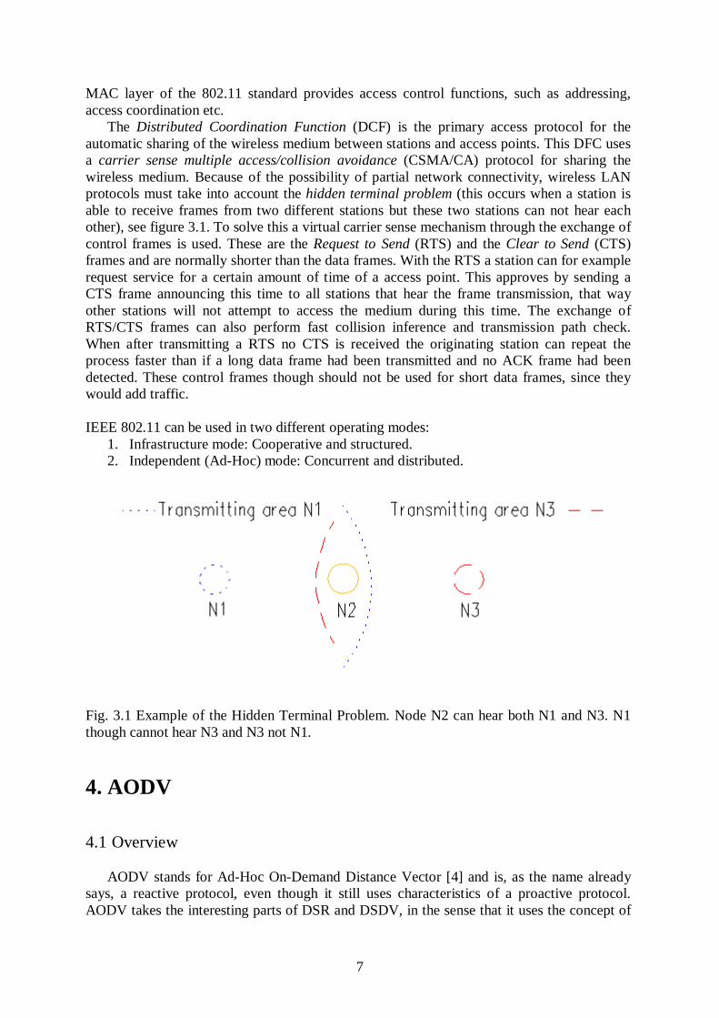
The Distributed Coordination Function (DCF) is the primary access protocol for the automatic sharing of the wireless medium between stations and access points. This DFC uses a carrier sense multiple access/collision avoidance (CSMA/CA) protocol for sharing the wireless medium. Because of the possibility of partial network connectivity, wireless LAN protocols must take into account the hidden terminal problem (this occurs when a station is able to receive frames from two different stations but these two stations can not hear each other), see figure 3.1. To solve this a virtual carrier sense mechanism through the exchange of control frames is used. These are the Request to Send (RTS) and the Clear to Send (CTS) frames and are normally shorter than the data frames. With the RTS a station can for example request service for a certain amount of time of a access point. This approves by sending a CTS frame announcing this time to all stations that hear the frame transmission, that way other stations will not attempt to access the medium during this time. The exchange of RTS/CTS frames can also perform fast collision inference and transmission path check. When after transmitting a RTS no CTS is received the originating station can repeat the process faster than if a long data frame had been transmitted and no ACK frame had been detected. These control frames though should not be used for short data frames, since they would add traffic.
IEEE 802.11 can be used in two different operating modes:
1. Infrastructure mode: Cooperative and structured. 2. Independent (Ad-Hoc) mode: Concurrent and distributed.
Fig. 3.1 Example of the Hidden Terminal Problem. Node N2 can hear both N1 and N3. N1 though cannot hear N3 and N3 not N1.
4. AODV 4.1 Overview
AODV stands for Ad-Hoc On-Demand Distance Vector [4] and is, as the name already says, a reactive protocol, even though it still uses characteristics of a proactive protocol. AODV takes the interesting parts of DSR and DSDV, in the sense that it uses the concept of

8
route discovery and route maintenance of DSR and the concept of sequence numbers and sending of periodic hello messages from DSDV.
Routes in AODV are discovered and established and maintained only when and as long as needed. To ensure loop freedom sequence numbers, which are created and updated by each node itself, are used. These allow also the nodes to select the most recent route to a given destination node.
AODV takes advantage of route tables. In these it stores routing information as destination and next hop addresses as well as the sequence number of a destination. Next to that a node also keeps a list of the precursor nodes, which route through it, to make route maintenance easier after link breakage. To prevent storing information and maintenance of routes that are not used anymore each route table entry has a lifetime. If during this time the route has not been used, the entry is discarded. 4.2 Route Discovery
When a node wants to communicate with an other node it first checks its own routing table if an entry for this destination node exists. If this is not the case, the source node has to initialize a route discovery. This is done by creating a RREQ message, including the hop count to destination, the IP address of the source and the destination, the sequence numbers of both of them, as well as the broadcast ID of the RREQ. This ID and the IP address of the source node together form a unique identifier of the RREQ. When the RREQ is created the source node broadcasts it and sets a timer to wait for reply.
All nodes which receive the RREQ first check by comparing the identifier of the message with identifiers of messages already received. If it is not the first time the node sees the message, it discards silently the message. If this is not the case the node processes the RREQ by updating its routing table with the reverse route. If a node is the destination node or has already an active route to the destination in its routing table with sequence number of the destination host which is higher than the one in the RREQ, it creates a RREP message and unicasts it to the source node. This can be done by analyzing the reverse route for the next hop. Otherwise it increments the RREQ’s hop count and then broadcasts the message to its neighbors.
When the source node receives no RREP as a response on its RREQ a new request is initialized with a higher TTL and wait value and a new ID. It retries to send a RREQ for a fixed number of times after which, when not receiving a response, it declares that the destination host is unreachable.
Fig. 4.2.1 shows the propagation of the RREQ through the network and the path taken by the RREP from the destination to the source node. 4.3 Route Maintenance
When a route has been established, it is being maintained by the source node as long as the route is needed. Movements of nodes effect only the routes passing through this specific node and thus do not have global effects. If the source node moves while having an active session, and loses connectivity with the next hop of the route, it can rebroadcast an RREQ. If though an intermediate station loses connectivity with its next hop it initiates an Route Error (RERR) message and broadcasts it to its precursor nodes and marks the entry of the destination in the route table as invalid, by setting the distance to infinity. The entry will only be discarded after a certain amount of time, since routing information may still be used.

9
Fig. 4.2.1 Propagation of RREQ and Fig. 4.3.1 Route Maintenance
Route Determination When the RERR message is received by a neighbor it also marks its route table entry for the destination as invalid and sends again RERR messages to its precursors.
In figure 4.3.1.I, the node N4 moves to N4’ and so node N3 can not communicate with it anymore, connectivity is lost. N3 creates a RERR message to N2, there the route is marked invalid and unicasts the message to N1. The message is unicast since we have only route passing through each node. N1 does the same thing and unicasts the message to the source node. When the RERR is received at the source node and it still needs the route to the destination it reinitiates a route discovery. Figure 4.3.1 II shows the new route from the source to the destination through node N5.
Also if a node receives a data packet for a node which it does not have an active route to, it creates a RERR message and broadcasts it as described above.
4.4 Hello Messages
If no broadcast has been send within, by default, one second, each node broadcasts Hello message to its neighbors in order to keep connectivity up to date. These messages contain the node’s IP address and its current sequence number. So that these messages are not forwarded from the node’s neighbors to third parties the Hello message has a TTL value of one.
5. Experimental Setup
In this chapter the system components, the software tools used to make the different experiments and the network setups for those experiments are described.

10
5.1 System components
To setup the MANET the following computers and laptop were used: Two stations using an AMD Athlon 900 MHz processor. They are equipped with the
standard I/O interfaces, such as serial and parallel ports, USB, CD-ROM, a keyboard and a mouse. Next to that they have a PCMCIA-to-PCI adapter installed. For the forced multihop experiments two more stations were used. On one is a Intel Pentium II 300 MHz processor installed and on the other a Intel Pentium III 450 MHz. They are also equipped with the standard I/O interfaces and a PCMCIA-to-PCI adapter.
In order to setup a MANET where the different nodes are not all inside the same collision domain, two laptops were used. One of them was a Toshiba 490 CDT laptop, using an Intel Pentium II processor and equipped with the standard I/O interfaces, and two Type I/II PCMCIA card slots. The other one a Toshiba 480 CDT laptop, with an Intel Pentium I processor and is equipped with the same interfaces as the other laptop.
On all of the stations and laptops is a Linux operating system running. The used Linux is the Red Hat Linux Version 7.3. An important character of Linux is that it includes TCP/IP networking software which were for this project indispensable .
The radio adapter chosen is the 2.4 GHz Wireless Lan Adapter of the Cisco Aironet 350 series [11]. Figure 5.1.1. shows a picture of the used radio adapter. Specifications related to them are shown in table 5.1.I.
Fig. 5.1.1 Wireless Lan Adapter, the PCMCIA version was used Table 5.1.I Cisco Aironet 350 Series Client Adapter Specifications
Data Rates Supported
1, 2, 5.5, and 11 Mbps
Network Standard IEEE 802.11b
Frequency Band 2.4 to 2.4897 GHz
Network Architecture Types
Infrastructure and ad hoc
Media Access Protocol
Carrier sense multiple access with collision avoidance (CSMA/CA)
Indoor:
130 ft (40 m) @ 11 Mbps
Range (typical)
350 ft (107 m) @ 1 Mbps

11
5.2 Software Tools
The software used during the project are noted and described in this section. 5.2.1 AODV-UU
AODV-UU [6] is the AODV implementation developed at the University of Uppsala, Sweden. For the experiments we used the, at the beginning of this project, latest version available, version 0.6. It is based on the AODV draft version 11.
AODV can be run, after installation, by typing the following command “./aodvd [options]” .
It is possible to log the routing table of AODV, this by using the option “-r 3”, where the number is the interval in seconds when a new log is made. For command line options run “./aodvd –help“. 5.2.2 AODV-UCSB
AODV-UCSB [7] is the AODV implementation developed at the University of California in Santa Barbara, USA. Version 0.1b is used for the experiments. It is based on the AODV draft version 10.
Use the command “./aodvd –o –t all” to run the daemon in the foreground with all the information concerning the routing printed to the screen. Use “./aodvd -?” for the command line options.
It has to be noted that AODV-UCSB uses partly files from the AODV-UU implementation. 5.2.3 PING
For different parts of the experiments the PING utility has been used. This software transmits by default one ICMP ECHO –REQUEST datagram per second, which asks for a ICMP ECHO-RESPONSE from the destination host. The output includes the datagram size, sequence number and the round trip time (RTT) of each request. When finished, PING prints out the minimum, average and maximum RTT and the packet loss statistics. By default we have a packet size of 56 bytes to which we have to count an addition 8 bytes used for the ICMP header. Thus we have by default 64 bytes inside the IP packet. The IP header measures without any options 20 bytes. The actual number of bytes leaving the IP layer is therefore 84 bytes.
ICMP [12] is the error and control message protocol used by the Internet protocol family. 5.2.4 NetPIPE
NetPIPE [8] stands for Network Protocol Independent Performance Evaluator. Version 3.3 has been used. This software is made to establish a connection, send and receive data and close the connection. It increases the to be transmitted data block size k from a single byte until transmission time exceeds one second or the block size reaches the defined upper limit. For each block size k three measurements are take, k - p bytes, k bytes and k + p bytes, where p is by default 3. NetPIPE produces a log file that contains the block size, throughput and transfer time. With those information it is for example possible to produce a graph that represents throughput versus the transfer block size. In our experiments NetPIPE was used to send and evaluate TCP traffic.

12
NetPIPE has to run on the two host. On the source node run “./NPtcp –t –h destination_node [options]”, where destination_node is the IP-address of this. On the destination node run “./NPtcp –r [options]” . 5.2.5 MGEN
MGEN [9] is a Multi-Generator Toolset, version 4 was used. MGEN is a Toolset to send
different packet sizes in a variety of ways, using UPD traffic over the network. To use MGEN on the sever side, scripts have to been written, in which you can define the port number from which the packets are send from, the IP address of the client node and the port number to which the packets have to be send to. Also the number of packets to send per second, the size of the packet, the way those packets have to be transmitted, either periodically or with a poison distribution, has to be defined. An example of such a script is:
“ 0.0 ON 1 UDP DST 192.168.100.1/5000 PERIODIC [1 1024] “
This script will originate a flow of MGEN UDP to the IP address 192.168.100.1 port number 5000 beginning immediately when the script is executed. The message will consist of 1024 byte messages at a regular rate of one per second.
On the client side it is possible to log the activities on the defined port. This log file gives us the following information: packet size, sequence number, time when packet was send, time when packet was received at the destination host, and IP address of the sending and receiver host. This log file is used to evaluate the throughput. The duration of each experiment will be defined in chapter 6. 5.2.6 Iptables
Iptables [10] gives us the functionality of packet filtering. This is done on the mac-layer. Iptables is included in the standard linux kernel.
The command to use to drop packets arriving from a specific node is:
“iptables –A INPUT -m mac --mac-source ab:cd:ef:gh:ij:kl –j DROP”
where ab:cd:ef:gh:ij:kl is the mac address of the node of which messages should be dropped. To see the list of mac addresses that are blocked type: “iptables –L” , for help “iptables --help”. 5.3 Set-up of the mobile Ad-Hoc network experiments
As described in the Introduction chapter of this paper two different scenarios were studied. In one we have a mobile Ad-Hoc network, where each node has exactly one up- and one downstream neighbor (when we have a link directed from node a to b, a is the upstream neighbor of b and b is the downstream neighbor of a). This scenario is a possible one of the reality. The disadvantage when doing experiments with such a network is that distances get with increasing number of hops fast extremely long. For this reason the network was, after performing the experiments in the real life scenario, moved into a room. There the first scenario was simulated by dropping on each node messages from other specified nodes, with which the node is not able to communicate with in reality.
13
5.3.1 Set-up of the real multihop experiments
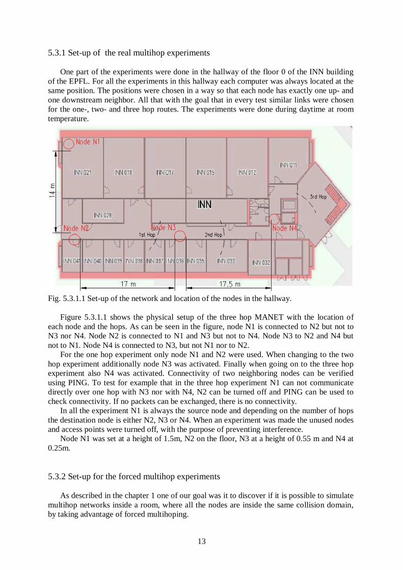
One part of the experiments were done in the hallway of the floor 0 of the INN building of the EPFL. For all the experiments in this hallway each computer was always located at the same position. The positions were chosen in a way so that each node has exactly one up- and one downstream neighbor. All that with the goal that in every test similar links were chosen for the one-, two- and three hop routes. The experiments were done during daytime at room temperature.
Fig. 5.3.1.1 Set-up of the network and location of the nodes in the hallway.
Figure 5.3.1.1 shows the physical setup of the three hop MANET with the location of each node and the hops. As can be seen in the figure, node N1 is connected to N2 but not to N3 nor N4. Node N2 is connected to N1 and N3 but not to N4. Node N3 to N2 and N4 but not to N1. Node N4 is connected to N3, but not N1 nor to N2.
For the one hop experiment only node N1 and N2 were used. When changing to the two hop experiment additionally node N3 was activated. Finally when going on to the three hop experiment also N4 was activated. Connectivity of two neighboring nodes can be verified using PING. To test for example that in the three hop experiment N1 can not communicate directly over one hop with N3 nor with N4, N2 can be turned off and PING can be used to check connectivity. If no packets can be exchanged, there is no connectivity.
In all the experiment N1 is always the source node and depending on the number of hops the destination node is either N2, N3 or N4. When an experiment was made the unused nodes and access points were turned off, with the purpose of preventing interference.
Node N1 was set at a height of 1.5m, N2 on the floor, N3 at a height of 0.55 m and N4 at 0.25m.
5.3.2 Set-up for the forced multihop experiments As described in the chapter 1 one of our goal was it to discover if it is possible to simulate
multihop networks inside a room, where all the nodes are inside the same collision domain, by taking advantage of forced multihoping.

14
Note also that this realization is a good and easy possibility to show students how mobile ad-hoc networking and AODV work, without having to set up each time a large network.
Fig. 5.3.2.1 Set-up in the laboratory room INN 021, the nodes where set at a height of 1.5 m When doing the experiments with forced multihoping we have to keep in mind that we
have only one collision domain. To avoid collision only one station can send at a time (CSMA/CA). When transmitting a package from the first node to the last in a three hop network the same phenomena can be observed in reality (RTS/CTS). When we have more than four nodes, forced multihoping does not reflect reality anymore, since in reality, if we have 5 nodes, the first node can transmit packages to the second node at the same time as the fourth node is transmitting packages to the fifth node.
After all the experiments done in a location where real multihoping is possible, in our case the hallway, were repeated in a room, the two obtained results were compared. In chapter 6 of this report the differences between the reality and the to each of them belonging forced multihop experiments are described. Below the exact order of events how forced multihoping can be set-up is described.
First of all, depending on the number of hops, a plan in which is defined which node is allowed to receive messages from which other nodes has to be drawn. See figure 5.3.2.2 for a possible example of such a three hop network.
Then on each node messages coming from machines that the node is not allowed to communicate with have to be dropped. This can be done using the iptables software and the command described in section 5.2.6. This command has to be repeated on each node for all the nodes that it is not allowed to communicate with. Now the multihop network is ready to be used.
Experiments were done at room temperature and during daytime. As nodes the four stations were used. The network set-up was the same as in the hallway, in the meaning that node N1 was always the sending node and depending on the number of hops N2, N3 or N4 was the receiving nodes. Figure 5.3.2.1 shows the physical set-up of the network in the INN 021 laboratory. All the precautions were made to avoid interference.
Note that for all the experiments made inside the laboratory and the hallway we use transmitting power of 1mW.

15
Fig. 5.3.2.2 Example of a 4 hop forced multihop set-up
5.3.3 Mobility experiment set-up
MANET and AODV are made for mobile scenarios and in real life they are also used under mobile circumstances. To test how mobility affects AODV mobile experiments were made. The set-up of those experiments is the same as in the hallway, shown in Figure 5.3.1.1. Node N1, N2 and N3 were the static nodes and have the same location as described above. N4 is the mobile source node.
Two different scenarios were tested. In the first scenario the position, where the node is being started to move, was the same position where node N4 was located in the hallway set-up. We approached then with slow walking speed (about 0.2 m/s) the destination node N1. The laptop was carried in the hands, which was at a height of 1.10 m. Before beginning to approach node N1 we waited for a stable connection. This to have for each experiment equal starting conditions.
In the second scenario the starting point was the destination node N1. This time instead of approaching the destination node, we walked away, with the sending node in the hands, from it. Conditions were the same as in the first scenario.
Comment on the set-up and the results: In order to be able to make exact comments on the results and what the connectivity and the RTT exactly depended on different important locations were noted on the results. These are the locations of the static nodes and the areas where each of the hop end.
6. Results and Comments
To evaluate the performance of AODV different experiments were performed under varying conditions. Our interests were:
• Route Discovery Time: The time taken from when a RREQ is assembled until the
RREP is received • Packet Loss Performance: The percentage of lost packages during 1000 ping • End-to-End Delay: The time taken from when a certain packet is sent by the
source node until it is received by the destination node • Communication Throughput using TCP and UDP traffic • Mobility: The behavior of AODV in the mobile case
The varying conditions were different route length, varying packet sizes and mobility.

16
All the different experiments were done in the hallway, where we have different collision domains and inside the laboratory, where we have only one collision domain, as described above.
We started with our experiments in the hallway and evaluated as first experiment the throughput using TCP. As described in chapter 1, one goal of the project was also to compare two implementation of AODV, namely AODV-UU and AODV-UCSB. So we performed the first experiments for both of the implementations. As can be seen in the results section for TCP, we found immense differences between the two implementation. Taking into account those facts we decided to adapt our project goals and continue the experiments only with the implementation of the University of Uppsala.
The different obtained results are discussed below. 6.1 Route Discovery Time
Whenever a node wants to communicate with another node and no entry in the routing table for this specific destination node exists, a route discovery is initiated. The time taken to discover this route is an important quality of a routing protocol.
Interesting to us was the time the UU implementation of AODV takes from when a RREQ is assembled until a RREP is received, what is called the Route Discovery Time (RDT). This time is in function of the distance to the destination and the size of the network (the number of nodes in the network), but does not depend on the size of the data packet to be transmitted.
For this experiment we used the same set-up as described in section 5.3.1. In order to measure the RDT the AODV-UU was started and its output was logged. AODV waits after reboot a certain period of time, called DELETE-PERIOD, before transmitting any route discovery messages, this is done since sequence numbers may be lost and routing loops may be created. Also after this period of time no neighboring node of the rebooted node will be using it as an active next hop any more.
After waiting the DELETE-PERIOD time we used PING to send a message to the destination node. The destination node was either N3 or N4, in function of the number of hops. The RDT for one hop was not tested, since during the DELETE-PERIOD the source node can receive Hello messages from its neighbors and therefore has a active route entry in the routing table of them. To be able to determine the RDT the routing table of the source node should only contain an entry for its neighboring node and no entry for the destination node should exist. This was the case, since no other nodes where having traffic, apart the normal AODV messages. It was also possible to consult the routing table of the sending node, before using PING, to verify that no entry for the destination node exists.
When the node is asked to transmit a message it first checks in its routing table if an entry for the destination node exists. If this is not the case it buffers the message and broadcasts a RREQ message. Only after the RREP message is received, the original to be transmitted message is sent. AODV notes in its output the time when an action occurred. By consulting this output it possible to determine the difference of time between the RREP was assembled and the RREQ was received. Figure 6.1.1 shows such a output. To have a good average of the RDT the proceedings described above where repeated 50 times for each network length of two and three hops.

17
Average RDT (ms)
Standard Deviation
2 Hop 80.49 41.87 3 Hop 177.42 66.51
Table 6.1.I Average RDT taken of 50 repetitions
For the average and the standard deviation the aberrant values were removed. The formula taken to determine if a value is aberrant is:
Q(3/4) + 1.5(Q(3/4) - Q(1/4)) > x aberrant, where Q(3/4) is the value situated at ¾ of the all values in ascend order.
Comments to the average RDT: If node N1 wants to know the route to node N3 it sends a
RREQ to its neighbors, which is in that case node N2. When node N2 receives the RREQ from N1 it checks its routing table to see if it has already a route to the desired destination node N3. Since N3 is a neighbor of N2, N2 has an entry for the desired node N3. So node N2 sends a RREP to N1 saying that the desired route goes through it. So in this set-up where we have a two hop route request, the RREQ has only to pass one hop.
20:28:59.896 host_init: Attaching to eth1, override with -i <if1,if2,...>. 20:28:59.954 aodv_socket_init: Receive buffer size set to 262144 20:28:59.954 main: In wait on reboot for 15000 milliseconds. Disable with "-D". 20:28:59.954 hello_start: Starting to send HELLOs! 20:29:00.952 rt_table_insert: Inserting 192.168.100.3 (bucket 3) next hop 192.168.100.3 20:29:00.952 rt_table_insert: New timer for 192.168.100.3, life=2100 20:29:00.952 hello_process: 192.168.100.3 new NEIGHBOR! 20:29:14.955 wait_on_reboot_timeout: Wait on reboot over!! 20:29:21.276 packet_queue_add: buffered pkt to 192.168.100.2 qlen=1 20:29:21.276 rreq_create: Assembled RREQ 192.168.100.2 20:29:21.276 log_pkt_fields: rreq->flags:GU rreq->hopcount=0 rreq->rreq_id=0 20:29:21.276 log_pkt_fields: rreq->dest_addr:192.168.100.2 rreq->dest_seqno=0 20:29:21.276 log_pkt_fields: rreq->orig_addr:192.168.100.1 rreq->orig_seqno=1 20:29:21.276 aodv_socket_send: AODV msg to 255.255.255.255 ttl=2 (28 bytes) 20:29:21.276 rreq_route_discovery: Seeking 192.168.100.2 ttl=2 20:29:21.431 rreq_process: ip_src=192.168.100.3 rreq_orig=192.168.100.1 rreq_dest=192.168.100.2 20:29:21.438 aodv_socket_process_packet: Received RREP 20:29:21.438 rrep_process: from 192.168.100.3 about 192.168.100.1->192.168.100.2 20:29:21.438 log_pkt_fields: rrep->flags: rrep->hcnt=2 20:29:21.438 log_pkt_fields: rrep->dest_addr:192.168.100.2 rrep->dest_seqno=11 20:29:21.438 log_pkt_fields: rrep->orig_addr:192.168.100.1 rrep->lifetime=1585 20:29:21.439 rt_table_insert: Inserting 192.168.100.2 (bucket 2) next hop 192.168.100.3 20:29:21.439 rt_table_insert: New timer for 192.168.100.2, life=1585 20:29:21.439 packet_queue_send: SENT 1 packets to 192.168.100.2 qlen=0
Fig. 6.1.1 An output of AODV- UU, taken when doing RDT experiments. The blue arrow represents the difference between the time the RREQ was assembled and the time the RREP was received.
18
For a three hop route request the RREQ has only to pass two hops. The results in table 6.1.I show that the RDT for a three hop route is a little more than the double of the RDT of a two hop route. That the RDT is not exactly linear can be explained by the fact that with every additional intermediate node in the route its IP address has to be recorded and therefore the RREP message is larger for a long route than for a shorter one.
We also note that the Standard Deviation is relatively high which is due to the channel conditions described in section 6.2. 6.2 Packet Loss Performance
Another important quality in communication is the packet loss performance of a network. It is influenced by factors like interference, multiple hops and channel conditions. In our experiments, as already mentioned, interference was as much as possible reduced and we want to measure to which degree multiple hops effect the packet loss performance in our two different set-ups.
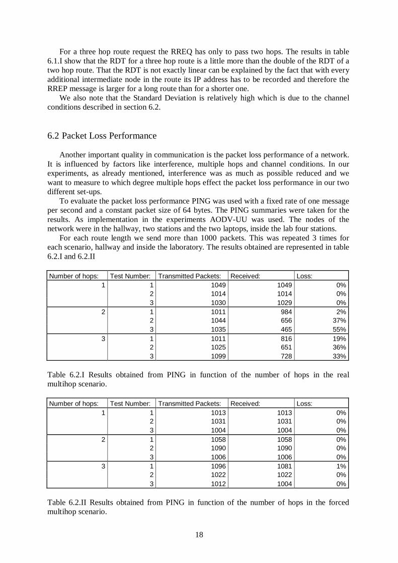
To evaluate the packet loss performance PING was used with a fixed rate of one message per second and a constant packet size of 64 bytes. The PING summaries were taken for the results. As implementation in the experiments AODV-UU was used. The nodes of the network were in the hallway, two stations and the two laptops, inside the lab four stations.
For each route length we send more than 1000 packets. This was repeated 3 times for each scenario, hallway and inside the laboratory. The results obtained are represented in table 6.2.I and 6.2.II
Number of hops: Test Number: Transmitted Packets: Received: Loss:
1 1 1049 1049 0% 2 1014 1014 0% 3 1030 1029 0%
2 1 1011 984 2% 2 1044 656 37% 3 1035 465 55%
3 1 1011 816 19% 2 1025 651 36% 3 1099 728 33% Table 6.2.I Results obtained from PING in function of the number of hops in the real multihop scenario. Number of hops: Test Number: Transmitted Packets: Received: Loss:
1 1 1013 1013 0% 2 1031 1031 0% 3 1004 1004 0%
2 1 1058 1058 0% 2 1090 1090 0% 3 1006 1006 0%
3 1 1096 1081 1% 2 1022 1022 0% 3 1012 1004 0% Table 6.2.II Results obtained from PING in function of the number of hops in the forced multihop scenario.

19
Inside the laboratory we have an excellent performance, as table 6.2.II shows. For one and two hops we have no packet losses and for three hops none or only few losses occurred. Packet loss performance depends on each single hop inside the route. The table shows increases in the number of losses with increasing number of hops. Therefore some packet losses are normal and we can not deduce from the results obtained in the forced multihop experiments a direct impact of AODV on the packet loss performance.
Table 6.2.I represents the results obtained in the real multihop experiments. It shows that for one hop we obtained almost the same results as for the experiments in the forced multihop experiments, which is normal, since the only difference between those two set-ups is the location of node N2. When the results for two and three hops are evaluated big differences to the forced mulithop experiment can be observed. Another striking observation are the differences from one performed test to the next, when the number of hops is constant. These differences can have several reasons. We have to take into account that the environmental conditions are not the same as inside the lab. People who walk in the hallway have a direct impact on the transmission of the electromagnetic waves. Another factor in the hallway was that the available space was limited and so the nodes where located near the end of the transmitting area of its neighboring nodes. Because of these factors link stability can vary from one test to the next.
This time also AODV may have a direct impact on the outcome. When no route to the destination exist, for example when waiting on the RREP message, the data packets waiting for the route are buffered. If a route discovery has been attempted RREQ_RETRIES, which is by default two, times without receiving a RREP, all the buffered data packets for this destination are dropped and a Destination Unreachable message is delivered to the application.
The conclusion of these experiments is that when simulating a multihop network by forcing multiple hops inside a room, packets have to be lost artificially, in order to make the results more realistic. 6.3 End-to-End Delay Performance The End-to-End delay is the amount of time taken from when a message has been sent by the source node until it is received by the destination node. It is the sum of the transmission, propagation, processing and queueing delay experienced by the message at every node of the network. This time is important since the shorter the EED of a message of a fixed size is, the higher the throughput. In our scenario the EED is influenced first of all by the Route Discovery Time. Since before the message actually can leave the source node, the node has to know a route to the destination node. Then another important influence of the EED when using AODV is the processing delay. When an intermediate node receives the message it first needs to analyze its header to see for whom the packet is destined for and then check for the node to which it has to forward the packet to. Another influence of the EED is for example mobility. When after mobility a connection to a node is lost, a new route has to be determined, which again adds a delay to the RTT. Here we do not take into account mobility and the Route Discovery Time. The EEDs were evaluated using NetPIPE. For each route length and scenario (real multihop and forced multihop) we repeated the experiments 20 times, this in order to get a better average. From the results of these experiments we could not only take the EED but also the saturation graph of the network. To obtain the saturation graph we plot the block size versus the transfer time and on both axis we use logarithmic scale. From this graph the saturation point, circled in the graph, can be obtained, after which an increase in block size results in an almost linear increase in

20
transfer time, this interval from the saturation point to the end of the graph is called the saturation interval. This means that after the saturation point an increase in the packet size does not result in an increase of the throughput anymore.
Saturation Graph of AODV- UU in the real multihop scenario
1
10
100
1000
10000
100000
0.001 0.01 0.1 1
EED in sec
Blo
ck s
ize
(byt
es)
One Hop Tw o Hop Three Hop
Fig. 6.3.1 Saturation Graph of experiments using AODV-UU in the real multihop network, in function of the block size and the number of hops From the figure 6.3.1, which represents the results from the experiments in a network with real multiple hops (described in section 5.3.1), we can see that there are two impacts on the EED. First of all the EED changes in function of the block size and secondly it depends on the route length.
Average EED for the real multihop scenario
Number of Hops Block size (bytes) 64 1024 32771
1 2.79 4.47 117.45
2 5.23 9.66 367.17 3 8.82 12.56 544.02
Table 6.3.I: The average End-to-End delay in the real multihop scenario for different block sizes in function of the route length.

21
To the impact of the block size: For block sizes from 1 to 771 bytes, the saturation point, we have an almost constant EED. What means, as can be seen in section 6.4 that in this interval we have a high increase in throughput (more data can be transmitted during the same amount of time). After the saturation point the EED increases almost linearly. There we have the saturation area, which can also be seen in the figure 6.4.2. Table 6.3.I represents the average EED delays of different block sizes.
When increasing the block size from 64 to 32771 bytes in a route length of 1 hop we have an increase of the EED from 2.79 ms to 117.45 ms, what equals to an average increase of 0.35 ms per 100 bytes. For a route length of 2 hops we have for the same block sizes as for 1 hop an increase of the EED from 5.23 to 367.17 ms, an average increase of 1.11 ms per 100 bytes. For the three hop route length the increase of the block size described above results in an increase of the EED from 8.82 to 544.02, equal to an average increase of 1.64 ms per 100 bytes.
To the impact of the route length on the EED: Since AODV is a routing protocol and therefore made for networks with multiple hops, it is interesting to see how the EED changes in function of the number of hops. In theory each additional hop should add the same amount of delay to the EED. If we take the block size of 64 bytes from the table 6.3.I we see that each additional hop adds about the EED of the 1 hop network to the EED, as predicted in theory. When looking at the block size of 1024 bytes, we the same rule can be observed.
Saturation Graph of AODV- UU in the forced multihop scenario
1
10
100
1000
10000
100000
0.001 0.01 0.1 1EED in sec
Blo
ck S
ize
(byt
es)
One Hop Tw o Hop Three Hop
Fig. 6.3.2 Saturation Graph of experiments using AODV-UU in the forced multihop network, in function of the block size and the number of hops

22
The same experiments were redone in a room where all the nodes are inside a collision domain, as described in section 5.3.2. Fig. 6.3.2 represents the results from this experiments. Also in these results we can observe the same characteristic as in the real multihop network. The EED changes in function of the block size and the route length. For all three hops we have up to a block size of 771 bytes a EED that changes not much from one block size to the next. Only the EED of the one hop network fluctuates, but if we take the average, it neither changes much up to a block size of 771 bytes. After this saturation point the EED grows nearly linear in function of the block size. When increasing the block size from 64 to 32771 bytes, we have for this scenario in the 1 hop network an average increase of 0.33 ms, for the two hop route 0.56 ms and for the three hop route 0.82 ms. This makes an increase factor from one to two hops of 1.70 and from one to three hops of 2.48.
The impact of the number of hops on the EED is at a block size of 64 bytes from one to two hops quite linear, as shown in table 6.3.II. That means for two hops the EED is approximately the double of the EED of the one hop route. When comparing the one hop route with the three hop one we notice a increasing factor of 7.1, instead of 3 predicted in the theory above. When looking at the EED for the different number at hops of a block size of 32771 bytes we have though a approximately linear increase from one route length to the next.
When comparing the two different scenarios, we see that the saturation graphs have the same form and have the same characteristics. When looking at the different EED we see that the EED of the forced multihop scenario performs better for one and two hops than the real multihop scenario. For three hops though we have for smaller block sizes a better performance in the real multihop scenario. This is due to the fact that at low block sizes no RTS/CTS messages are used and therefore N4 can send to N3 at the same time as N1 to N2 without collisions occur. This is not possible in the forced multihop scenario.
Conclusion of this experiment is that the forced multihop scenario can be used to simulate the real multihop scenario when we are interested in the different characteristics of the network. Since for example the saturation points lie in the same area and also additional delays from one route length to the next are in both scenarios similar.
Average EED for the forced multihop scenario
Number of Hops Block size (bytes) 64 1024 32771
1 2.42 5.51 111.33 2 4.02 7.82 187.05 3 17.5 22.22 286.17
Table 6.3.II: The average End-to-End delay in the forced multihop scenario for different block sizes in function of the route length. 6.4 Throughput using TCP traffic
Another important quality of communication networks is the throughput, since it can for example effect the performance of applications. Therefore it is interesting to have a high throughput. It is defined as the total useful data received per unit of time.

23
The idea of these experiments was to investigate how route length and data block size effect the communication throughput, when using AODV as the routing protocol and sending TCP traffic. Note that the packet size is the sum of the data block and the header size.
To evaluate the throughput performance of our networks NetPIPE was used. For each route length we repeated the experiments 20 times, this in order to get a better average. The experiments in the multihop scenario were done in a first time using AODV-UCSB and in a second time using AODV-UU. In the results of these experiments a big difference between the performances of these two implementations can be seen, for which reason we decided to perform the remaining experiments only with the AODV implementation of UU anymore. In the multihop scenario again the two stations and two laptops were used, in the forced multihop scenario the four stations. The set-ups are described in sections 5.3.1 and 5.3.2.
Figure 6.4.1 represents the results obtained from the experiments using AODV-UCSB in the hallway, the real multihop scenario, in function of the data block size and the number of hops.
First we would like to discuss the impact of the data block size on the throughput. In theory is predicted that the throughput changes when increasing the data block size. The explanation for this is that there is a difference in sending a packet with 1 byte data and a header 64 times or sending a packet with 64 bytes data and a header of the same size as before one time. In the sense that for example in the larger packet we have only one processing delay and by sending the smaller packet 64 times we have that amount of times the processing delay. The obtained results show also this fluctuating of the throughput when changing the block size.
Here we have to note that unfortunately it was not possible to get results for three hops. We were able to ping the destination node N4 from the source node N1, but experienced many packet losses and large delay. NetPIPE therefore was not able to establish a connection.
Throughput Diagram AODV- UCSB TCP in the real multihop scenario
0
0.2
0.4
0.6
0.8
1
1.2
1.4
1.6
1.8
0 5000 10000 15000 20000 25000 30000 35000
Block Size (Bytes)
Thro
ughp
ut (M
bps)
One Hop Tw o Hops
Fig. 6.4.1 Throughput diagram of the experiments made with AODV-UCSB in the hallway, with a real multihop network, in function of the block size and the number of hops
In the one hop experiment when using AODV-UCSB and increasing the data block size from 64 to 1021 bytes we have an increase of the throughput from 0.119 to 1.417 Mbps,

24
which is equal to an increase of 1090.8 % in the throughput. After that peak the throughput falls again to 0.769 Mbps at a block size of 1533 bytes. The maximum throughput is reached at a block size of 4093 bytes with a value of 1.544 Mbps. When a block size of 6141 bytes is reached the throughput only fluctuates minimal anymore and saturates at 1.25 Mbps.
For two hops we have a similar impact of the block size on the throughput. The diagram for two hops has two similar peaks of the throughput performance as discussed for the one hop diagram. The values for those two peaks are at a block size of 1027 bytes 0.201 Mbps and at a block size of 4099 bytes 0.280 Mbps, which is the maximum throughput for the two hops experiment. It is interesting to observe that the two peaks are around the same block sizes. The two hop graph also saturates after reaching a block size of 6141 bytes at a throughput value of about 0.2 Mbps.
The conclusion is that by increasing block size we can increase the performance of throughput in this set-up. By using large block sizes two main problems can occur. First of all if a bit error occurs a large amount of data has to be retransmitted. Secondly, in our experiment there was just one source node, but in other networks it may be possible that many nodes want to send at the same time therefore contention may occur and it is possible that unfairness is observed. Thus the maximizing block size of these experiments can not be generalized for other MANET set-ups.
To the impact of the number of hops on the throughput for the experiment with AODV-UCSB in the hallway. Since every additional hop increases the probability of packet loss, as seen in the results of section 6.2, and adds a delay, due to transmission, propagation, processing and queuing, we have to observe a diminution of the throughput by increasing the number of hops. In theory throughput diminishes with a factor is O(1/n) of the one hop throughput, where n is the number of hops in the route. In the results of our experiments we have for example at a block size of 1027 bytes by switching from one to two hops a reduction of the throughput of a factor of 6.37, which is very poor.
We then performed the same experiments described and discussed above, but this times we used instead of AODV-UCSB the implementation of UU, AODV-UU. The results obtained are represented in figure 6.4.2. By analyzing the results the same phenomena of the throughput performance varying in function of the block size can be observed. For the one hop results we have by increasing the block size from 64 to 1021 bytes an increase of the throughput from 0.182 to 1.782 Mbps, which is equal to an increase of 879% in the throughput. After a fall in the throughput performance to 1.282 Mbps at a block size of 1536 bytes, we have again a rise to a maximum of 2.264 Mbps at a block size of 4093 bytes. After this value the throughput saturates at around 2.15 Mbps. Here it is interesting to observe that the saturation value is close to the maximum value. For a route length of two and three hops the graphs have a similar form as the one for one hop. We reach the maximum throughput for the two hop route at a block size of 4093 bytes, which was already the size that maximized the throughput for the one hop route, with a value of 0.939 Mbps. The throughput saturates at a value of about 0.75 Mbps. For the three hop route the throughput maximizing block size is again 4093 bytes with a value of the throughput of 0.758 Mbps. It saturates at a value of about 0.55 Mbps.
A note on the maximum throughput. The reason why the maximum throughput is lower than the transmission rate of 11 Mbps for the 802.11b protocol is that our throughput is the pure data throughput (without headers) at the network layer. The 11 Mbps is the absolute throughput at the physical layer including for example headers.
A note on the saturation point. It is interesting to compare the saturation point seen in figure 6.3.1 with the one from figure 6.4.2. The throughput of the saturating block size, 771 bytes, of figure 6.3.1 is close to the saturating throughput in figure 6.4.2. The maximum throughput is though close to this saturating throughput. Also in figure 6.3.1 we can observe that not all the values are exactly on the linear line.

25
The conclusion is as described for the experiment with AODV-UCSB that by increasing the block size we can increase the throughput, but we have to find an optimum in order to prevent problems like contention, as described above. For this set-up the optimum block size would be 4093 bytes for all three route lengths.
The influence of every additional hop in the route on the throughput is here again good observable. As already described above we observe with every additional hop a greater delay and more packet losses. Here we would like to compare if the diminishing factor of the throughput of the different route lengths follows the theoretical one. For that we take the maximizing block size of 4093 bytes for all three route lengths. The throughput values for this specific route length are for one hop 2.264, for two hops 0.939 and for three hops 0.758 Mbps. By switching from one to two hops in the route length we have a diminution of the throughput of a factor 2.41 and by switching from one to three hops a factor of 2.99. In this experiment the diminishing factor is for two hops much closer to the theoretical one than the one observed in the AODV-UCSB experiment and for three hops the diminution factor is almost equal to the theoretical one.
Throughput Diagram AODV- UU TCP in the real multihop scenario
0
0.5
1
1.5
2
2.5
0 5000 10000 15000 20000 25000 30000 35000
Block Size (Bytes)
Th
rou
gh
pu
t (M
bp
s)
One Hop Tw o Hop Three Hop
Fig. 6.4.2 Throughput diagram of the experiments made with AODV-UU in the real multihop scenario in function of the block size and the number of hops
These results are again only valid for this set-up and it is possible that if we have a
network with more nodes and higher traffic the resulting graphs may look different and the diminishing factor for example can be much higher. This can happen if in a three hop set-up the last link is also used by other nodes as a route.
26
For the experiments made in the forced multihop scenario we used the set-up described in section 5.3.2. In order to make the experiments NetPIPE was used and the experiments were for each route length repeated 20 times.
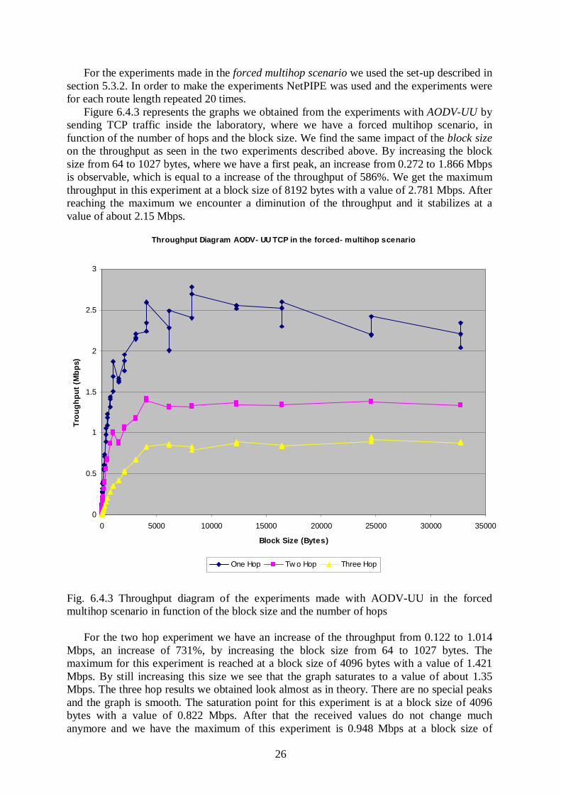
Figure 6.4.3 represents the graphs we obtained from the experiments with AODV-UU by sending TCP traffic inside the laboratory, where we have a forced multihop scenario, in function of the number of hops and the block size. We find the same impact of the block size on the throughput as seen in the two experiments described above. By increasing the block size from 64 to 1027 bytes, where we have a first peak, an increase from 0.272 to 1.866 Mbps is observable, which is equal to a increase of the throughput of 586%. We get the maximum throughput in this experiment at a block size of 8192 bytes with a value of 2.781 Mbps. After reaching the maximum we encounter a diminution of the throughput and it stabilizes at a value of about 2.15 Mbps.
Throughput Diagram AODV- UU TCP in the forced- multihop scenario
0
0.5
1
1.5
2
2.5
3
0 5000 10000 15000 20000 25000 30000 35000
Block Size (Bytes)
Tro
ug
hp
ut
(Mb
ps)
One Hop Tw o Hop Three Hop
Fig. 6.4.3 Throughput diagram of the experiments made with AODV-UU in the forced multihop scenario in function of the block size and the number of hops
For the two hop experiment we have an increase of the throughput from 0.122 to 1.014 Mbps, an increase of 731%, by increasing the block size from 64 to 1027 bytes. The maximum for this experiment is reached at a block size of 4096 bytes with a value of 1.421 Mbps. By still increasing this size we see that the graph saturates to a value of about 1.35 Mbps. The three hop results we obtained look almost as in theory. There are no special peaks and the graph is smooth. The saturation point for this experiment is at a block size of 4096 bytes with a value of 0.822 Mbps. After that the received values do not change much anymore and we have the maximum of this experiment is 0.948 Mbps at a block size of

27
24576 bytes. We also have to mention that the graphs for two and three hops saturate quite fast and that the values we received for block sizes above the saturation point do not deviate much from the value in the saturation point, which is not the case in the one hop results.
By looking at those three results it is again observable that there is no point in increasing the block size to large sizes. This would have, as seen for the one hop, opposite effects and we would have to observe a smaller throughput as would be possible to obtain. These results are obtained from the experiments made and would be different if we have more nodes and the traffic is high. In networks with high traffic there is even less a point in increasing the block size to large values, for reasons described above.
When analyzing the effect of the route length on the throughput we can again observe that every additional hop adds delay to the packet and thus the result is a diminution in the throughput. If we compare the three result obtained at the block size of 4099 bytes, we have for one hop a throughput of 2.597, for two hops 1.395 and for three hops 0.828 Mbps. The diminution factor from one to two hops is 1.86 and from one hop to three hop it is 3.14. The values obtain are close to the theoretical values and thus confirm them for those experiments.
Comparison of the AODV implementations of UCSB and UU
0
0.5
1
1.5
2
2.5
0 5000 10000 15000 20000 25000 30000 35000
Packet Size (Bytes)
Th
rou
gh
pu
t (M
bp
s)
UU 1 Hop UU 2 Hop UCSB 1 Hop UCSB 2 Hop
Fig. 6.4.4. Comparison of the throughput of the AODV implementations made by UU and UCSB
It is also interesting to make a comparison of the experiments made in the real multihop scenario with the two different implementation, figure 6.4.4 represents this. Three main characteristics come to mind. First of all we can see that all the graphs have a similar form. All of them have a steep increase in the throughput at the beginning, then they all have a first

28
peak at the block size region of 1021, 1024, 1027 bytes (NetPIPE makes for each block size k three measurements at k - 3, k , k + 3 bytes). After this first peak all three graphs have a decrease in throughput around the block size of 1536 bytes. After a second peak, at around the block size of 4096 bytes, all four graphs saturate. The second fact we notice is that the region where we have this second peak is for all four graphs the block size value that maximizes the throughput value.
What is the most noticeable however is the difference between the throughput values of the two implementations. To compare the four graphs we take their throughput values at the block size of 4093 bytes. The value at this block size for AODV-UU one hop is 2.264, for two hop it is 0.939, for AODV-UCSB one hop it is 1.494 and for two hops it is 0.277 Mbps. We have therefore at this block size for AODV-UU one hop a 51.57 % higher throughput value than for the same set-up with the AODV-UCSB implementation. For the two hop set-up the throughput value of the AODV-UU implementation is even 238.99 % higher than the same for the AODV-UCSB implementation. These results, and the fact that we could not get any results for AODV-UCSB three hops, contrary to the same set-up for AODV-UU, show us that the implementation of AODV developed at the University of Uppsala has, for our experiments, a much better performance than the one developed at the University of California at Santa Barbara. We can see that even if two implementations make use of the same algorithm, we have big differences in the results. Implementation therefore matters a lot and has a big influence on the outcome of a algorithm. As a result of the differences between the two implementations described above, we decided to perform the remaining experiments only with AODV-UU anymore. 6.5 Throughput using UDP traffic
Next to the throughput using TCP traffic we were also interested in the throughput with UDP traffic. For this experiment we used MGEN to produce the traffic and the log file. To have an average we let run the experiment for 180 seconds. UDP throughput was measured in the hallway, with a real multihop network, and inside the laboratory, with a forced multihop one. This is done for one, two and three hops, using AODV-UU and all the experiments were repeated for different sending rates, in the diagram called ‘offered load’ and route lengths. The sending rates were: 0.1 * i Mbps, where i є [1,15] and the packet size was kept fix at a value of 1472 bytes. The exact set-ups of the networks are described in sections 5.3.1 and 5.3.2.
Figure 6.5.1 represents the offered load versus the received load of the experiments described above obtained in the hallway. The diagram shows that the received load of one hop follows up to an offered load of 0.7 Mbps almost the ideal case, that means that the received load is equal to the offered load. And also for higher offered load still a high percentage of it is received. For two and three hops though the received load starts already to drop at low offered loads. At a offered load of 1.1 Mbps in the two hop network 0.76 Mbps are received, what is equal to 69.09 % of the offered load, in the three hop network 0.67 Mbps (60.9 %). The saturation point is located at a offered load of 1.3 Mbps.
It is remarkable that the graphs of two and three hops have, up to a offered load of 1.3 Mbps, a similar form. To explain this result we should know where exactly the packets are lost. A possible explanation is that already at the sending node problems of route discovery come up. When on two sent Route Discoveries no answer is received all the buffered messages, which are waiting for a established route, are dropped. The chance of a packet loss increases with the sending rate, what means that with higher rate the probability that a AODV control message is lost increases and therefore also more buffered packets are drop. This explains for one part why at high rates proportional less data is received at the destination

29
node. Another explanation of the similar form for the two and three hop graphs is that only a small portion of the sent data is received at the third node and therefore the chance of lost packets is smaller for the last hop. Another is the hidden terminal problem. For example nodes N1 and N3 send both UDP messages, either AODV control messages or data messages, but they cannot hear each other. The maximal offered load, for two and three hops, at which all the data is received at the destination node is 0.2 Mbps.
Throughput Diagram AODV- UU UDP in the real multihop scenario
0
0.2
0.4
0.6
0.8
1
1.2
1.4
1.6
0 0.2 0.4 0.6 0.8 1 1.2 1.4 1.6
Offered Load (Mbps)
Rec
eive
d L
oad
(M
bp
s)
1 Hop 2 Hop 3 Hop
Fig. 6.5.1 Throughput Diagram with UDP traffic when using AODV-UU in the real multihop scenario.
Figure 6.5.2 represents the offered load versus the received load of the experiments described above obtained inside the laboratory room. Here is remarkable how well the one and two hops set-ups perform. At a offered load of 1.2 Mbps for the one hop network we have a received load of 1.12 Mbps and for two hops 1.10 Mbps. Only at higher offered rates a drop in the received load is observed. The reason for such a good performance are as shown in section 6.2 the perfect packet loss performance for one and two hops, the good link quality and the fact that, due to CSMA/CA, only one station can transmit packets at a time, thus we have for example no AODV control messages lost. What is interesting to see in the results of the performed experiments, is that for the offered loads of 1.3 up to 1.5 Mbps the two hop set-up has a better performance than the one hop set-up. First of all we have to say that both perform good and we do not have a big difference between the two obtained results. Another point is that more repetitions should be performed to see if this is a constant case. To explain this case we should know where exactly the packets were lost. Another problem is that the experiments were redone for each route length. Better would have been if we used directly

30
the three hop route and logged at each node the received load. That way it could not have happened that the two hop route as a higher received load than the one hop.
The three hops performs up to a sending rate of 0.7 Mbps almost ideal. When increasing the sending rate a sudden drop is observed. The reason for that is, as already described, at high frequencies the probability of a packet loss is higher and therefore also the packet loss of AODV control messages is higher, which is even increased with higher number of hops. A repeated loss of AODV control message has a drop of the buffered message as consequence.
Throughput Diagram AODV- UU UDP in the forced multihop scenario
0
0.2
0.4
0.6
0.8
1
1.2
1.4
1.6
0 0.2 0.4 0.6 0.8 1 1.2 1.4 1.6
Offered Load (Mbps)
Rec
eive
d L
oad
(M
bp
s)
1 Hop 2 Hop 3 Hop
Fig. 6.5.2 Throughput Diagram with UDP traffic when using AODV-UU in the forced multihop scenario. 6.6 Mobility
Mobile Ad-Hoc networks are, as the name says, mobile. The nodes of such a network may be in constant movement, possible routes from one node to another may change constantly and therefore it is important that an algorithm like AODV takes these cases into account and reacts fast on mobility, route errors and lost connectivity. The goal of this part of the project was to evaluate AODV in the mobile scenario. Unfortunately material and labor was limited and we could just evaluate two cases possible in mobility.
For this experiment we used the set-up described in section 5.3.3 with the AODV implementation of UU. In order to measure connectivity and the RTT in the mobile case,

31
PING was used on the mobile node N4 and we pinged the destination node N1. PING was configured to send one message per second with a size, as described in section 5.2.3, of 64 bytes inside the IP packet. The size and the sending rate was kept at a constant value during each and for all the experiments. This does not reflect reality, but in this exercise we wanted to keep our interests on the pure effects of mobility on the connectivity.
The experiments of the first scenario were repeated 12 times and the experiments of the second scenario three times. We came to the conclusion that it does not make sense to take an average of the different results, since all the results obtained look different one from another and they do not follow a specific form. For this reason we like to show and discuss here two results obtained from the experiments of the first scenario and one from the second scenario. Figure 6.6.1 represents the results from the eight experiment made in the first scenario. In this figure the zones are highlighted where I started walking, passed hop number 2, as shown in figure 5.3.1, node N3, hop number one, node N2 and where I arrived at the destination node N1.
The packets that have their RTT entry at 100 ms have either a RTT of 100 ms or more or are lost packets, this was done to make the diagram more readable. First we describe the obtained graph. Before starting to walk with the node in the hand a wait was held for 10 seconds (10 packets sent) to stabilize the connection. Then we started to walk with a speed of about 0.2 m/s. What is observable is that there are 22 lost packets out of 143 sent ones, which are 15.38 %. This value is in our opinion, quite low if compared to the results seen in table 6.2.I.
Mobility Experiment Number 8 (Approaching the destination node N1)
0
20
40
60
80
100
120
1 7 13 19 25 31 37 43 49 55 61 67 73 79 85 91 97 103
109
115
121
127
133
139
Packet Number
RT
T (
ms)
Hop 2Start Node N3 Hop 1 Node N2 Node N1
Fig. 6.6.1 Dynamics of the RTT in the mobility scenario, source node N4 approaches destination node N1

32
We thought about how the diagram should look like in theory (with no packet loss) for those experiments and came to two possibilities. One possibility is that when connectivity with the initial next hop is lost the sending node searches a new route and therefore we have at that moment a sudden increase in the RTT and after this peak there should be a decrease in the RTT again until it stabilizes. More optimal and realistic would be though when getting into the communication area of a node that is closer to the destination than the actual next node in the routing table, therefore when changing the number of hops to destination, the sending node should find a new route through this new neighboring node of his. At those moments we would experience the same phenomena as described in the first possibility. No special occurrence should happen in theory when passing directly by a node.
When looking for reasons for a packet loss, we have to keep in mind that the loss of a packet can always have different reasons. The first lost packets (number 17 – 26) are normal lost packets, which easily occur as seen in the PING results for three hops. When passing hop number two we experience a packet loss, which is explainable with the second possibility we found in the theoretical course of events. We change to a new neighboring node (this can be detected by node N4 when receiving a hello message from the new neighboring node) and have to find a new route through it, which is done by sending a RREQ. During this period of time a packet loss is possible when no answer is received on two RREQ.
Mobility Experiment Number 14 (Approaching the destination node N1)
0
20
40
60
80
100
120
1 9 17 25 33 41 49 57 65 73 81 89 97 105 113 121 129 137 145 153 161 169
Packet Number
RTT
(ms)
Node N3Start Hop 2 Hop 1 Node N2 Node N1
Fig. 6.6.2 Dynamics of the RTT in the mobility scenario, source node N4 approaches destination node N1
Note also that there are no special events when passing node N3, which is also in theory
like that. The next packet losses occur when switching from two hops to one hop. This means that now we can directly communicate with the destination node N1. By the fact that we now

33
have to send the packets directly to N1 and not anymore to an intermediate node leads temporary to an increase of the RTT. This since this change has first to be noticed and evaluated. In this experiment this changing of the hop and possible other reasons, like normal packet losses, lead here to packet losses.
Inside the one hop area no special events, next to two lost packets, occur anymore. This makes sense since we have no change of hop anymore and communicate directly with the destination node N1.
By analyzing the results another characteristic was noticed. By approaching the destination node, we have in areas with a stable connection, a decrease in the RTT. Which is explainable with the fact that with fewer intermediate nodes in the route we have less delay added.
Another outcome is represented in figure 6.6.2. Here we have, contrary to figure 6.6.1, almost no areas where we have a stable connection, only when close to the destination node a stability is reached. The form of the graph is chaotic and is only explainable with a bad connection and many general packet losses.
Out of the 12 mobility experiments made in this set-up five had a chaotic form with many packet losses and seven had a nice form as seen in figure 6.6.1.
Figure 6.6.3 shows us the graph from the experiment number nine, where we walked with the source node N4 in the hands away from the destination node N1. The set-up and the method how to send the pings was the same as described in the first scenario.
Mobility Experiment Number 9 (Walking away from the destination node N1)
0
20
40
60
80
100
120
1 9 17 25 33 41 49 57 65 73 81 89 97 105 113 121 129 137 145 153 161
Packet Number
RTT
(ms)
Hop 2Node N2 Hop 1 Node N3Start at Node N1 End
Fig. 6.6.3 Dynamics of the RTT in the mobility scenario, source node N4 walks away from destination node N1

34
In this graph we also have many packet losses (42 out of 161 sent packets, 26.09%), but there is still a certain form to see in it. At the beginning, when close to the destination, we have a stable connection and the RTT is low. The further away we get from node N1 the less stable the connection is and packets start to get lost. Around the area where passing hop number one we have many changes between lost and arrived packets. Connectivity here is not stable. Also when passing hop number two we have a whole range of lost packets, this is also due to the hop switch as described in the theory part above. After this range we have a relatively stable connection with only some packet losses anymore. It is again observable that RTT is in general higher when far away from the destination node than when close to it.
All three experiments done in this second scenario have about the same form. Our general opinion about these experiments done is that we can observe a similarity with
the possible theoretical outcome. As already observed in the packet loss performance experiment, section 6.2, we have a big diversion in the number of lost packets from one experiment to another. This explains the different outcomes seen in figure 6.6.1 and 6.6.2. If we take though an experiment with few packet losses as seen in figure 6.6.1 AODV-UU reacts very good to mobility! Unfortunately from this same figure it is not possible to say how fast exactly AODV-UU reacts on the hop switch, therefore finds a new route through the new neighboring node, since we can see when passing hop number two we only have one lost packet and when passing hop number one we have nine lost packets.
Here we also have to note that the results found here reflect only the set-up described in section 5.3.3 and that the results would also be different when using another implementation of AODV than the one from UU.
Although we have mobility in those experiments, they still only reflect a part of the reality, since in other networks it is possible that all the nodes are mobile and there can be many more nodes than only four like in this experiment. To have all this was unfortunately not possible to be done, since labor and material was limited. Next to that we also should do more experiments with for example a higher sending rate and packet size than taken in this set-up. That way it would be possible to make a more general opinion about how AODV behaves on mobility.
7. Conclusion
In this project, the performance evaluation of the AODV routing protocol in Mobile Ad-Hoc Network in real multihop scenarios, an important kind of evaluation was done since reality is reflected. This report presents the results we obtained from our experiments to evaluate AODV, where we set our interest on Route Discovery Time, Packet Loss Performance, End-to-End delay, Communication Throughput and Mobility.
We compared the results of experiments done in a real multihop scenario with the one obtained in a forced (all the nodes are inside the same collision domain) multihop scenarios and came to interesting conclusions.
Two different implementations of the same algorithm were compared and we found that not only it is important to have a good algorithm, but also the implementation contributes significantly to the success of it.
The differences between the two compared implementation of the AODV routing protocol, AODV–UU and AODV–UCSB, are, as shown in figure 6.4.4, impressive. In our experiments the differences get, with increasing route length, the more and more important, until in the three hop scenario, NetPIPE was not even able anymore to get a throughput from AODV-UCSB.
From the results of the experiments performed under forced multihop conditions we can conclude that this kind of scenario can very good be used to simulate the real multihop

35
network for up to three hops and also for example for teaching purposes. This since the different results and graphs have similar characteristics and forms. Only the packet loss performance is much better in the forced multihop, due to the good channel conditions. This packet loss can be simulated be artificial packet drops.
The real multihop performance of AODV-UU are in our experiments partially very promising. The diminishing factor of the communication throughput with TCP traffic, as shown in figure 6.4.2, from one route length to the next, follows the theoretical factor of O(1/n), where n is the number of contenders, in our experiments the number of hops in the route. This is an important character of a routing protocol. We also found that the data block size has a high impact on the throughput and the end-to-end delay.
The communication throughput for multiple hops with UDP traffic starts only to diminish significantly for high offered loads, this due to the higher packet loss probability with increasing sending rate and number of hops in the route. This can lead to losses of AODV control messages and drops of buffered messages. The packet loss performance, shown in table 6.2.I, fluctuated a lot from one performed experiment to the next and depends therefore significantly on the channel conditions. Some outcomes of the experiments were not encouraging. Reason for that are mainly the constraints under which we set-up our network.
In some obtained results in the mobility scenario are good and AODV reacts fast on mobility and route losses. In other experiments we have many packet losses even in areas where we have no route losses or next hop changes. This can be lead back to the different outcomes done in the packet loss performance experiments and the channel conditions.
Based on the results obtained in our experiments we can say that AODV should not be used for multimedia application but for example for wireless sensor networks and that the performance of AODV-UU is acceptable and encouraging.

36
8. Bibliography [1] D. Johnson et al., Dynamic Source Routing for Mobile Ad Hoc Networks, IEFT MANET Draft, April 2003 [2] Charles E. Perkins, Destination- Sequence Distance- Vector Protocol, Ad Hoc Networking, ISBN 0-201-30976-9, pp. 53- 74 [3] C.-K. Toh, Associativity- Based Routing, IEEE Transactions on wireless communications, Vol. 1, No. 3, July 2002 [4] Charles E. Perkins, Elizabeth M. Belding-Royer, Samir R. Das
Ad hoc On-Demand Distance Vector Routing, IEFT MANET Draft, February 2003 Charles E. Perkins, Ad Hoc Networking, ISBN 0-201-30976-9 [5] Jim Geier, Wireless LANs, ISBN 0-6723-2058-4 [6] Implementation of AODV, Uppsala University,
http://user.it.uu.se/~henrikl/aodv/index.shtml [7] Implementation of AODV, University of California, Santa Barbara,
http://moment.cs.ucsb.edu/AODV/aodv.html [8] NetPIPE, http://www.scl.ameslab.gov/netpipe/
Quinn O. Snell, Armin R. Mikler, John L. Gustafson, NetPIPE: A Network Protocol Independent Performance Evaluator
[9] MGEN, http://mgen.pf.itd.nrl.navy.mil/mgen.html [10] Iptables, http://www.netfilter.org/ [11] Cisco wireless adapters, http://www.cisco.com [12] J. Postel, Internet Control Message Protocol, IETF Internet RFC 792, 1981