performance evaluation of mpe rainfall product at hourly and daily temporal resolution within a

Performance Evaluation of MPE Rainfall Product at Hourly and Daily Temporal Resolution within a Hydro-Estimator Pixel1

Alejandra M. Rojas-González 2, Eric W. Harmsen3 and Sandra Cruz Pol4

2Graduate student, Department of Civil Engineering, University of Puerto Rico,

Mayagüez, PR 00681, USA [email protected]

3Professor, Department of Agricultural and Biosystems Engineering, University of Puerto Rico

Mayagüez, PR 00681, U.S.A. [email protected]

4Professor, Department of Computer and Electrical Engineering, University of Puerto Rico

Mayagüez, PR 00681, U.S.A [email protected]

ABSTRACT: A rain gauge network (28 rain gauges) was installed in western Puerto Rico (PR) within a 4km x 4km GOES satellite pixel. Located within the pixel is a well monitored sub-watershed of 3.55 km2, referred to here as the “testbed subwatershed” (TBSW). The rain gauge network was established to evaluate rainfall estimates from the GOES-based Hydro-Estimator (HE), NEXRAD radar and the Center for Collaborative Adaptive Sensing of the Atmosphere (CASA) radar network, which has a high spatial resolution (≈ 200 m). Furthermore, the rain gauge network will provide a high temporal and spatial resolution rainfall dataset to be input into a distributed hydrologic model in the TBSW.

The focus of this work is to evaluate the performance of the Multisensor Precipitation Estimation (MPE) product at 1-hour and 1-day temporal resolution within the 4km x 4km HE pixel for 2007. The MPE product is popular within the hydrologic modeling community due to its resolution and mean field bias correction computations in its coverage.

Results for 2007 indicate that the highest rainfall measured by the rain gauges within the HE pixel area were September with an average and standard deviation of 241.75 mm and 73.3 mm, respectively; and August with 223.7 mm and 64.66 mm, respectively. While for the same months the MPE, produced a total monthly rainfall accumulation and standard deviation of 247.36 mm and 64.4 mm for September, respectively, and 233.68 mm and 36.54 mm for August, respectively. The mean and standard deviation daily field bias for these months were 1.08 and 1.5 for September, respectively, and 0.93 and 1.6 for August, respectively. The bias changed, when considering an hourly analysis, to 1.98 average and 5.45 standard deviation for August and 1.49 average and 3.01 standard deviation for September. Nevertheless the month that produced the largest mean bias was November with 2.24, and 2.6 standard deviation for daily rainfall accumulations; and a mean bias of 3.92 and 8.16 standard deviation for an hourly time step. In this study percentages of detection and false alarms were determined at two time scales. Key-Words: - Multisensor Precipitation Estimation, NEXRAD products, rainfall variability, mean field bias.

1. INTRODUCTION In western Puerto Rico a study is being conducted to develop a Doppler and polarimetric radar network operating with a frequency of 9.41

gigahertz (X band). This radar network will provide an effective way to predict the weather conditions in western Puerto Rico at a high spatial

WSEAS TRANSACTIONS on ENVIRONMENT and DEVELOPMENTAlejandra M. Rojas-Gonzalez, Eric W. Harmsen, Sandra Cruz Pol

ISSN: 1790-5079 478 Issue 7, Volume 5, July 2009

resolution, and will provide precipitation estimates for flood forecasting models.

A major source of error in hydrologic models is the poor quantification of the areal distribution of rainfall, typically due to the low density of rain gauges. A rain gauge located at a single point may represent an extensive area, typically > 107 m2, with only one value, which much of the time is not representative of the average rainfall, especially in areas of high topographic variability subject to convection storms [1]. Rain gauges themselves may produce errors, a major source of error being from turbulence and increased winds around the gauge, affecting precipitation quantification in events where the wind is an important factor (e.g., hurricanes).

Investigators have used mean areal precipitation as calculated by, for example Thiessen polygons, [1,2], and interpolation methods, such as spline, inverse distance weighted, and kriging. But all these methods are limited by the number of rain gauges and how they represent the spatial rainfall distribution. Currently, sophisticated methods attempt to fill gaps between rain gauges, by sensing the atmosphere with remote sensors like the space-borne Tropical Rainfall Measuring Mission (TRMM), the National Oceanic and Atmospheric Administration’s (NOAA) Hydro Estimator (HE) algorithm [4], the satellite precipitation estimation /radar rainfall merging algorithm of the NOAA-CREST Group at City University of New York [5], the U.S. National Weather Service’s (NWS) Next Generation Radar (NEXRAD), and the Multisensor Precipitation Estimation Algorithm (MPE). The HE utilizes data from the GOES geostationary satellite to estimate rainfall, and has, for example, an approximate pixel size of 4km x 4km. NEXRAD estimates rainfall within a radial coordinate system with a base resolution of 2 to 4 km.

These quantitative precipitation estimation (QPE) techniques are evaluated and adjusted or calibrated using existing rain gauges, however, these adjustments depend on the rain gauge density and their spatial distribution. Studies that have compared radar and rain gauge–derived rainfall documented large discrepancies between them [e.g., 6,7,8].

The MPE algorithm is a product of NEXRAD, and recently has replaced the Stage II and III algorithms. MPE is based on multi-year climatology of the Digital Precipitation Array (DPA) product (hourly and 4km x 4km resolution) and performs a mean field bias correction over the entire radar coverage area, based on (near) real-time hourly rain gauge data [9]. The MPE is mapped onto a polar stereographic projection called the Hydrologic Rainfall Analysis Project (HRAP) grid. This data is often used in the hydrologic modeling availing the bias correction made by the MPE algorithm; nevertheless, in long term hydrologic simulations and watersheds with small numbers of rain gauges a bias verification would be evaluated, because the bias quantification has a high variability over the radar coverage area [10,11] affecting the hydrologic calibration and validation.

With the objective to calibrate and validate the high density CASA radar network in western PR, a rain gauge network (28 tipping buckets rain gauges) was installed in a small highland area. The rain gauge network is located within a single 4km x 4km GOES HE pixel and 12 of the 28 rain gauges are within the testbed subwatershed (TBSW). The rain gauge network will provide a high resolution rainfall data set to evaluate the CASA radars, calculate the NEXRAD products and Hydro Estimator uncertainty under their typical resolution [10], and understand the hydrologic response and predictability limits due to rainfall and topographic resolution using a distributed hydrologic model to capture the spatial variations. The TBSW has an area of 3.55 km2, belongs to the Río Grande de Añasco watershed, has an average 29% slope, the predominant soil hydrologic group is C, and the surface soil has an average 3.25 cm/hr hydraulic conductivity. For long term simulations a bias evaluation was developed in this study for use in the hydrologic modeling. 2. METHODOLOGY In this study, the performance of the MPE product within the HE pixel for 2007 was evaluated using the rain gauge network (26 rain gauges) located in western Puerto Rico near the University of Puerto Rico – Mayaguez Campus. In 2006, sixteen



tipping bucket rain gauges (Spectrum Technology, Inc.1) were installed uniformly within the Hydro-Estimator (HE) pixel [10]. In June 2007, another 12 tipping bucket rain gauges were added to the network located within the TBSW.

The maximum, average and standard deviation distance between the 28 rain gauges calculated using Euclidian Distance are 829 m, 334 m and 171 m, respectively. These statistical parameters were reduced within TBSW as follows: 563 m, 218 m and 100 m, respectively. Fig. 1, shows the rain gauge network, the TBSW outline and the distance between rain gauges.

Fig. 1. Rain gauge distribution and location within the HE pixel, TBSW location and Euclidean Distance between the stations.

Some rain gauges were not operating during some periods owing to gauge damage or low logger batteries, these data were eliminated from the analysis. Five-minute rain gauge data was accumulated to 1-hour and 1-day intervals, with the intention to comparing data with the original MPE temporal resolution and daily accumulations.

MPE pixels are based on a HRAP grid. Therefore, a geographic coordinate transformation from Stereographic North Pole to NAD 1983 State Plane Puerto Rico and Virgin Islands was performed for each hour using the ArcGIS project

1 Reference to a commercial product in no way constitutes an endorsement of the product by the authors.

raster tool. The re-sampling technique algorithm used was the nearest neighbor assignment at 4km x 4km resolution. Due to changes in coordinates and raster conversions, the original pixels oriented with a certain angle, now are oriented horizontally. Figure 2 displays the change in the orientation, including the MPE pixels (left) and Hourly Rainfall Product (N1P) from NEXRAD level 3 (right). The left image shows four square black boxes corresponding to the MPE raster-projected pixels, the colored pixels are the original raster with HRAP coordinates at 4km x 4km spatial resolution, and the red box corresponds to the Hydro-Estimator pixel at the same resolution as the MPE product.

Fig. 2. MPE pixels (left) at different geographic coordinates and the HE pixel (red box). Hourly rainfall product from NEXRAD level 3 (right) as a shapefile and raster format. The TBSW is also shown near the center of the four MPE pixels.

The N1P rainfall product is calculated from NEXRAD as a rain rate each 5 or 6 minutes when the radar detects rainfall, and a 10 minutes N1P product is archived when no rainfall is detected. The N1P NEXRAD product has originally a polar geographic coordinate system (GCS) and using the NOAA Weather and Climate Toolkit Exporter program it is possible to transform the coordinates to GCS_WGS_1984. Different formats are available to export the data. The shapefiles maintain the original orientation; however, in a distributed hydrologic model it is necessary to use raster or ASCII files to represent the spatial rainfall variation in the model. Due to raster characteristics it is not possible to maintain the original orientation. Fig. 2, right image, shows the shapefile in black lines and a rainfall raster as colored pixels, both at 2km x 2km resolution.

Pixel 1 Pixel 2

Pixel 3 Pixel 4



The study was made with the projected and raster pixels, with the aforementioned in mind, 4 MPE pixels were obtained around the HE pixel, identified as Pixel 1 (top left), Pixel 2 (top right), Pixel 3 (bottom left) and Pixel 4 (bottom right), Fig. 2 (left). Area weights were calculated for intersecting areas between the MPE pixels and the HE pixel and are 0.281, 0.344, 0.169 and 0.206, respectively. These area weights are used to calculate an average map precipitation for each time step. Weights for the N1P radar product were also estimated for 9 partial N1P pixels within the HE pixel (Fig. 2, left).

2.1 Analysis

Validation of the radar products have to be evaluated to improve the hydrologic simulation. Long term continuous validation between sensors rainfall estimates and rain gauge observations should be evaluated. The accuracy of rainfall estimates can be measured by decomposing the rainfall process into sequences of discrete and continuous random variables [11,12].

The discrete variables can be evaluated with contingency tables, where the rain gauges are the “ground truth” values and the MPE are the estimated values. In this way, the accuracy of the rainfall detection in terms of hit rate “H”, probability of detection “POD”, false-alarm rate “FAR” and discrete bias “DB” can be evaluated.

Table 1 shows an example of two-way contingency tale. The variable a is the number of times that the rain gauge identifies a rainfall event and the estimator also correctly identifies a rainfall event at the same time and space. The variable d represents the number of times the rain gauge does not observe a rainfall event and the estimator correctly determines that there is no rainfall event. The variable b indicates the number of times the rain gauge does not observe a rainfall event but the estimator incorrectly indicates that there is a rainfall event. The variable c shows the number of times that the rain gauge detects a rainfall event but the estimator fails to detect the rainfall event [11].

Hit rate (H) is the fraction of the no estimating occasions when the categorical estimation correctly determines the occurrence of rainfall event or nonevent. Probability of detection (POD) is the likelihood that the event

would be estimated, given that it occurred. The false-alarm rate (FAR) is the proportion of estimated rainfall events that fail to materialize. Bias is the ratio of the number of estimated rainfall events to the number of observed events [12]. Table 1. Two-way contingency table. Observed Rainfall

(Rain gauges) Yes No

Estimated MPE Rainfall

Yes a b No c d

The typical scores that measure the accuracy of categorical estimation are:

,0n

daH

+= where dcbano +++= (1)

ca

aPOD

+= (2)

ba

bFAR

+= (3)

ca

baDB

++= (4)

The mean field bias (Bias) is used to

remove systematic error from radar estimates and used to correct the radar quantifications in the hydrologic simulation. The mean field bias is defined as the ratio of the “true” mean areal rain gauge rainfall to the corresponding radar rainfall accumulations. [13,14]. The average of the rain gauge network is evaluated each time step with a arithmetic mean, because the area weights change in time according to malfunctions in some gauges. The mean MPE rainfall at each time step is calculated using the area weights as stated above.

The indicators to evaluate the accuracy of MPE rainfall estimations over the HE pixel at different temporal scales are the Bias, root mean square error (RMSE) and normalized bias (NBIAS).



∑

∑

=

==t

t

N

ii

N

ii

R

GBias

1

1

(5)

( )2

1

1

21

−= ∑

=

tN

iii

t

RGN

RMSE (6)

( )

∑

∑

=

=

−

=t

t

N

ii

t

N

iii

t

GN

RGN

NBIAS

1

1

1

1

(7)

Where Nt is the number of hours, Gi is the areal mean rain gauge-based rain rate value at time i, and Ri is the corresponding areal mean radar rain rate value.

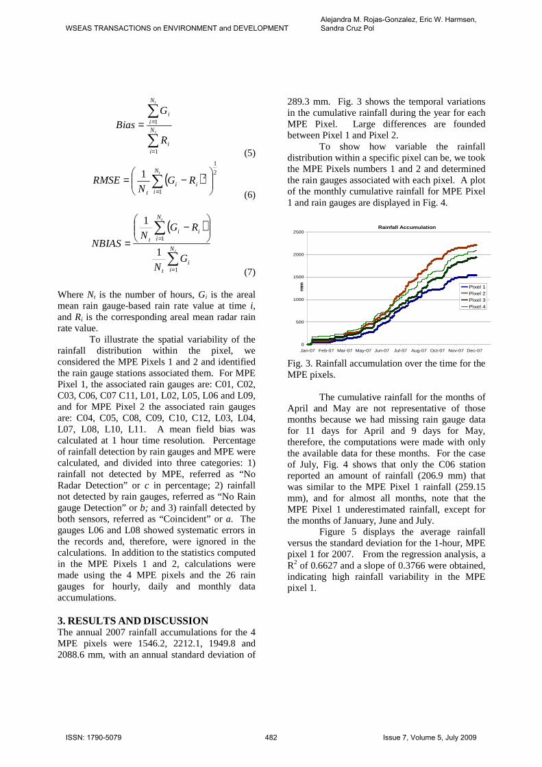
To illustrate the spatial variability of the rainfall distribution within the pixel, we considered the MPE Pixels 1 and 2 and identified the rain gauge stations associated them. For MPE Pixel 1, the associated rain gauges are: C01, C02, C03, C06, C07 C11, L01, L02, L05, L06 and L09, and for MPE Pixel 2 the associated rain gauges are: C04, C05, C08, C09, C10, C12, L03, L04, L07, L08, L10, L11. A mean field bias was calculated at 1 hour time resolution. Percentage of rainfall detection by rain gauges and MPE were calculated, and divided into three categories: 1) rainfall not detected by MPE, referred as “No Radar Detection” or c in percentage; 2) rainfall not detected by rain gauges, referred as “No Rain gauge Detection” or b; and 3) rainfall detected by both sensors, referred as “Coincident” or a. The gauges L06 and L08 showed systematic errors in the records and, therefore, were ignored in the calculations. In addition to the statistics computed in the MPE Pixels 1 and 2, calculations were made using the 4 MPE pixels and the 26 rain gauges for hourly, daily and monthly data accumulations. 3. RESULTS AND DISCUSSION The annual 2007 rainfall accumulations for the 4 MPE pixels were 1546.2, 2212.1, 1949.8 and 2088.6 mm, with an annual standard deviation of

289.3 mm. Fig. 3 shows the temporal variations in the cumulative rainfall during the year for each MPE Pixel. Large differences are founded between Pixel 1 and Pixel 2.

To show how variable the rainfall distribution within a specific pixel can be, we took the MPE Pixels numbers 1 and 2 and determined the rain gauges associated with each pixel. A plot of the monthly cumulative rainfall for MPE Pixel 1 and rain gauges are displayed in Fig. 4.

Rainfall Accumulation

0

500

1000

1500

2000

2500

Jan-07 Feb-07 Mar-07 May-07 Jun-07 Jul-07 Aug-07 Oct-07 Nov-07 Dec-07

mm Pixel 1

Pixel 2Pixel 3Pixel 4

Fig. 3. Rainfall accumulation over the time for the MPE pixels.

The cumulative rainfall for the months of

April and May are not representative of those months because we had missing rain gauge data for 11 days for April and 9 days for May, therefore, the computations were made with only the available data for these months. For the case of July, Fig. 4 shows that only the C06 station reported an amount of rainfall (206.9 mm) that was similar to the MPE Pixel 1 rainfall (259.15 mm), and for almost all months, note that the MPE Pixel 1 underestimated rainfall, except for the months of January, June and July.

Figure 5 displays the average rainfall versus the standard deviation for the 1-hour, MPE pixel 1 for 2007. From the regression analysis, a R2 of 0.6627 and a slope of 0.3766 were obtained, indicating high rainfall variability in the MPE pixel 1.



Rainfall Totals per month in the MPE Pixel 1

0

50

100

150

200

250

300

350

Jan-07 Feb-07 Mar-07 Apr-07 May-07

Jun-07 Jul-07 Aug-07 Sep-07 Oct-07 Nov-07 Dec-07

Rai

nfa

ll (m

m)

C01 C02 C03 C06 C07 C11 L01 L02 L05 L06 L09 Pixel 1 Fig. 4. Monthly Total Rainfall calculation for the rain gauge stations belongs to MPE Pixel 1, for 2007.

MPE Pixel 1

y = 0.35x + 0.04R2 = 0.64

0.00

5.00

10.00

15.00

20.00

25.00

30.00

0.00 10.00 20.00 30.00 40.00 50.00

Average Rainfall (mm)

Sta

nd

ard

Dev

iati

on

(m

m)

Fig 5. Hourly average and standard deviation rainfall for the rain gauges corresponding to MPE pixel 1 for the 2007.

4 MPE Pixels

y = 0.60x + 0.03R2 = 0.78

0.00

5.00

10.00

15.00

20.00

25.00

30.00

0.00 5.00 10.00 15.00 20.00 25.00

Average Rainfall (mm)

Sta

nd

ard

Dev

iati

on

(m

m)

Fig 6. Hourly average and standard deviation rainfall for the rain gauges corresponding to 4 MPE pixels for the 2007.

The rainfall detection variability

decreases when the four pixels are averaged by

their HE weights as mentioned above. The linear regression indicates a R2 of 0.78 and a slope of 0.60 (Fig. 6).

Mean rain gauge data and mean weighted MPE rainfall were graphed at the hourly time step and a linear regression equation was calculated (Fig. 7) obtaining a slope line of 0.508 and a R2 of 0.43.

Hourly Measurements

y = 0.5081x + 0.1542R2 = 0.4307

0

5

10

15

20

25

30

35

40

45

50

0 5 10 15 20 25 30 35 40 45 50

Rain Gauge average (mm)

MP

E P

ixel

s av

erag

e (m

m)

Fig.7. Average rain gauge rainfall vs. MPE radar rainfall within HE pixel at hourly time step.

The contingency tables and scores (Tables 2 and 3, respectively) were calculated to evaluate the Pixel 1, Pixel 2 and total 4 MPE pixels for hourly time step and daily rainfall accumulations for the four MPE pixels within the HE pixel. The number of estimated rainfall events were overestimated according to the discrete bias (DB) in the MPE pixel 1 (1.24) comparing with the Pixel 2 and the 4 MPE pixels, which have a values close to 1. For daily data the DB is underestimated by a factor of 0.956. The hit rate (H) indicates the occasions when the categorical estimation correctly determined the occurrence of rainfall event or nonevent and was around 0.82 and 0.89; non-significant differences were found between hourly and daily accumulations.

Moreover, the probability of detection (POD) is the likelihood that the event would be estimated by the radar, increasing with the time step, with 0.833 for the daily data. Daily estimates eliminate the influence of light rainfalls that the radar cannot detect. For the hourly time step, the Pixel 1 POD was higher than the POD for Pixel 2 and the average of 4 MPE pixels.

False alarm rates or portion of estimated rainfall events that fail to materialize are similar in Pixels 1, 2 (0.50 and 0.42 respectively) and the four pixels average (0.45). For the daily time step



there was a considerable reduction in the FAR (0.128). Table 2. Contingency tables for the MPE pixels.

Hourly Data MPE Pixel 1 Observed Rainfall



Yes 638 653 No 400 6581

Hourly Data MPE Pixel 2 Observed Rainfall



Yes 630 464 No 449 6729

Hourly Data 4 MPE Pixels

Observed Rainfall (Rain gauges)

Yes No Estimated MPE

Rainfall Yes 915 756 No 693 5910

Daily Data 4 MPE Pixel

Observed Rainfall (Rain gauges)

Yes No Estimated MPE

Rainfall Yes 225 33 No 45 341

Table 3. Discrete validation scores for the MPE pixels and time scales. Hourly Data Daily Data

MPE

Pixel 1 MPE

Pixel 2 4 MPE pixels

4 MPE pixels

POD 0.62 0.58 0.57 0.833 FAR 0.51 0.42 0.45 0.128 DB 1.24 1.01 1.04 0.956 H 0.87 0.89 0.82 0.879

Figures 8 and 9 show the distribution of

false alarms and the probability of no detection by the radar during 2007. Events in which the radar did not detect rainfall and the rain gauges did measure rainfall (c) were assigned a value of 1 in the graph. Events in which the radar did detected rainfall and the gauges did not measure rainfall (b) were assigned a value of 2. Differences in time when false alarms and probability of no detection quantities occurred can be observed in the graphs, and detailed statistics are presented in Table 3 and 4.

False Alarm at Pixel 1

0

1

2

1/1/

07

2/1/

07

3/1/

07

4/1/

07

5/1/

07

6/1/

07

7/1/

07

8/1/

07

9/1/

07

10/1

/07

11/1

/07

12/1

/07

Null Radar Detection (c) Null Gauge Detection (b) Fig.8. Hourly False Alarm Time Series for the MPE Pixel 1 for 2007.

False Alarm at HE pixel

0

1

2

1/1/

07

1/15/

07

1/29/

07

2/12

/07

2/26

/07

3/12/

07

3/26

/07

4/9/

07

4/23

/07

5/7/

07

5/21

/07

6/4/0

7

6/18

/07

7/2/

07

7/16

/07

7/30

/07

8/13

/07

8/27/

07

9/10/

07

9/24

/07

10/8

/07

10/2

2/07

11/5

/07

11/19

/07

12/3

/07

12/1

7/07

12/3

1/07

Null Radar Detection (c) Null Gauge Detection (b) Fig.9. Hourly False Alarm Time Series for the MPE Pixels within a HE Pixel for June to December 2007.

A mean field bias (Bias) was calculated for the MPE Pixel 1, 2 and overall 4 pixels, as the ratio of the average of the rain gauge rainfall and the mean rainfall sensed for the MPE pixels using the area weights for each time step (hourly, daily, monthly and annually accumulations). Hourly mean field bias time series are displayed in the Fig. 10 (MPE Pixel 1) and Fig. 11 (mean four MPE pixels into the HE pixel).

Large biases were found at the hourly time step and are associated with small radar rainfall and rain gauge detections (Fig. 10). Because, the minimum precipitation depth that the radar is capable of detecting is 0.01 inches or 0.00394 mm; while our rain gauge network has a rainfall depth resolution of 0.1 mm. The NEXRAD in Puerto Rico is located about 100 km from the study area in Cayey at a site elevation of 850 meters msl. Due to the earth curvature, the



beam has an elevation of 600 m above site at Mayagüez, affecting the cloud’s measurements in the lower troposphere.

To neutralize the noise effect of little rainfall quantifications in the hourly bias computation, rainfall depths less that 0.3 mm were eliminated. A considerable hourly bias reduction was observed in time (Fig. 12) and in the average and standard deviation computation across the year as well as monthly (Table 3 and Table 4).

The continuous validation scores for MPE rainfall validation (Table 4) show a normalized bias of -0.151 for daily and -0.17 for hourly accumulations. The root mean square error is greater (0.368) in daily accumulations than in hourly (0.012). The mean field bias average over 2007 in the Pixel 1 is 3.85 with a standard deviation average of 4.21 mm. The 4 MPE pixels present less Bias (2.77) but a large standard deviation (8.18). The annual average Bias is improved after eliminating rainfall depths less that 0.3 mm, diminishing to 1.55 and a standard deviation of 2.14.

In the months of April and May some data in the rain gauge network were missing, and as a consequence, the mean field bias was calculated only for the existing data. In addition, the MPE Pixels present the complete accumulations for these months while the rain gauge column shown only the exiting data. The MPE total accumulations are 120.9 and 187 mm for April and May (Table 5), but the MPE accumulations only for the time window that correspond to the rain gauge data are 22.41 and 143.61 mm for April and May, respectively.

The mean field bias tended to decrease when the calculation was performed for the whole HE pixel area (16 km2). Therefore when the MPE is accumulated (e.g., over several hours or days) the bias is reduced and the standard deviation as well. Table 5 provides detailed bias computations for 2007.

Table 4. Continuous validation scores for the MPE pixels and time scales.

Mean Hourly

Daily Data

MPE Pixel

1

MPE Pixel

2

4 MPE pixels

4 MPE pixels Rain≥

0.3mm 4 MPE pixels

NBIAS - - -0.17 - -0.151 RMSE - - 0.012 - 0.368 Bias 3.85 1.58 2.77 1.55 1.23 STD Bias

4.21 2.73 8.18 2.14 1.65

Mean Field Bias in Pixel 1

0.001

0.01

0.1

1

10

100

Jan-07Feb-07

Mar-07

Apr-07

May-07Jun-07

Jul-07Aug-07

Sep-07Oct-0

7Nov-07

Dec-07Jan-08

Bia

s

Fig.10. Hourly Mean Field Bias for the MPE Pixel 1 for 2007 year.

Mean Field Bias at HE pixel

0.001

0.01

0.1

1

10

100

Jan-07Feb-07

Mar-07

Apr-07

May-07Jun-07

Jul-07Aug-07

Sep-07Oct-07

Nov-07Dec-07

Jan-08

Bia

s

Fig.11. Hourly Mean Field Bias for the four MPE Pixels for 2007 year within a HE Pixel.



Mean Field Bias at HE pixel without rain less than 0.3mm

0.01

0.1

1

10

100

Jan-07Feb-07

Mar-07

Apr-07

May-07Jun-07

Jul-07Aug-07

Sep-07Oct-07

Nov-07Dec-07

Jan-08

Bia

s

Fig.12. Hourly Mean Field Bias for the overall MPE Pixels within a HE Pixel for June to December 2007.

The results indicate that the month with largest hourly bias was December (5.68), which also had the highest variability (STD =12.92). These results are decreased to 1.53 and 2.52 respectively, when the average rainfall less than 0.3 mm in radar and rain gauges were eliminated. The greatest daily Bias occurred in November with 2.24 and a standard deviation (STD) of 2.6. The months with Bias close to 1 are June, July, August and September of which only August and September maintain the value close to one in monthly accumulations.

Table 5. Total rainfall in the MPE pixels and mean field daily bias calculation.

MPE Pixel Rainfall MPE Statistics Rain

Gauge Month Daily Bias Hourly Bias Hourly Bias Rain>0.3mm

1 2 3 4 Mean STD Total Bias Mean STD Mean STD Mean STD

(mm) (mm) (mm) (mm) (mm) (mm) (mm) (mm) (mm) (mm) (mm) (mm) (mm)

Jan 45.3 77.3 110.4 179.2 94.9 57.3 15.51 0.16 1.43 1.81 2.47 4.77 0.60 2.02

Feb 39.9 72.6 53.0 54.9 56.5 13.4 71.50 1.27 1.20 1.91 2.89 9.11 2.57 2.80

Mar 59.5 106.7 56.6 74.8 78.4 23.0 94.62 1.21 1.36 1.38 1.48 1.89 2.18 1.98

Apr 91.6 129.5 128.4 140.7 120.9 21.3

May 142.8 203.2 182.7 223.7 187.0 34.5

Jun 220.5 283.3 196.0 206.0 235.0 39.2 192.01 0.82 1.02 0.85 3.25 10.59 1.26 1.44

Jul 259.2 430.3 245.7 263.5 316.6 87.4 82.22 0.26 0.97 1.51 1.04 2.68 0.39 0.88

Aug 200.4 268.2 195.9 252.6 233.7 36.5 223.69 0.96 0.93 1.60 1.98 5.45 1.66 2.44

Sept 164.4 312.4 277.9 227.1 247.4 64.4 241.45 0.98 1.08 1.50 1.49 3.01 1.61 1.58

Oct 177.2 187.9 261.9 239.2 208.0 40.6 204.23 0.98 0.72 0.50 1.14 1.74 1.19 0.99

Nov 89.2 72.2 124.4 117.4 95.1 24.4 162.49 1.71 2.24 2.60 3.92 8.16 2.92 4.55

Dec 55.7 68.0 111.7 104.0 79.4 27.2 109.86 1.38 1.72 2.38 5.68 12.92 1.53 2.52

Year 1545.7 2211.4 1944.4 2083.2 1952.7 249.8 1542.3 0.85 1.24 1.65 2.77 8.14 1.55 2.14

4. CONCLUSIONS The Multi-sensor Precipitation Estimation algorithm was developed by the U.S. National Weather Service to improve the NEXRAD rainfall quantifications applying an hourly bias correction over the radar coverage. In western Puerto Rico the rain gauge density to correct the MPE algorithm is poor and the bias calculated can not be applied to this region or to small watersheds, incorporating errors into hydrologic simulations. In this study, the MPE algorithm was evaluated at a small-scale within a Hydro-Estimator pixel associated with 4 MPE pixels. Individual and

overall MPE pixels were evaluated at different time scales. At major time scales (daily) the MPE performed better, except for the months of January, July, November and December comparing them with the monthly mean field bias. The hourly Bias computation for January and July presented in the Table 5 could be improved by eliminating light rainfall less than 0.3 mm in the radar and rain gauge averages. Monthly Bias variations exist in the average MPE pixels compared to the ratio of average rain gauge network and total annual MPE rainfall at 4 pixels (0.85).



A future study should extend the area to cover not only the TBSW but also the rain gauges that are in the Río Grande de Añasco and Guanajibo basins to validate the MPE algorithm and correct the rainfall quantification by a new bias factor in the hydrologic modeling.

NEXRAD Level 3 (N1P) quantification will be performed and compared with the rain gauge network data, generating surfaces at each time step within the HE pixel and the TBSW. It is imperative to measure the performance of the QPE at scales below the 2km x 2km (N1P) resolution and quantify how the hydrologic response is affected by temporal and spatial precipitation resolutions.

Acknowledgements Financial support was received from and NSF-CASA and NOAA-CREST (NA17AE1625). References [1] Wilson, J. W. and E. A. Brandes, 1979: Radar

measurement of rainfall –A summary. Bulletin of the AMS, Vo.l. 60., Issue 9, Sept., pp 1048-1058.

[2] Viessman, W., and G. L. Lewis, 1996: Introduction to Hydrology. 4th Edition, Harper-Collins, 760 pp.

[3] Stellman, K.M., H.E. Fuelberg,, R. Garza, M. Mullusky, 2001: An Examination of Radar and Rain Gauge–Derived Mean Areal Precipitation over Georgia Watersheds. American Meteorological Society Journal. Volume 16, Issue 1, February 2001.

[4] Scofield, R.A. and R.J. Kuligowski, 2003: Status and outlook of operational satellite precipitation algorithms for extreme-precipitation events. Wea, Forecasting, 18, 1037-1051.

[5] Mahani, S. E., and R. Khanbilvardi, 2009. Generating Multi-Sensor Precipitation Estimates over Radar Gap Areas. WSEAS Transactions on Systems. Vol. 8, pp. 96-106.

[6] Baeck, M. L., and J. A. Smith, 1998: Estimation of heavy rainfall by the WSR-88D. Weather Forecasting, 13, 416–436.

[7] McGregor, K. C., R. L. Bingner, A. J. Bowie, and G. R. Foster, 1995. Erosivity index values for northern Mississippi. Trans. ASCE, 38, 1039–1047.

[8] Woodley, W. L., A. R. Olsen, A. Herndon, and V. Wiggert, 1975: Comparison of gauge and radar methods of convective rain measurement. J. Appl. Meteor., 14, 909–928.

[9] Seo, D.J, J. P. Briedenbach, and E. R. Johnson, 1999: Real-time estimation of mean field bias in radar rainfall data. J. Hydrol., 223, 131–147.

[10] Harmsen, E. W., S. E. Gomez Mesa, E. Cabassa, N. D. Ramirez Beltran, S. C. Pol, R. J. Kuligowski ,R. Vasquez, 2008. Satellite Sub-Pixel Rainfall Variability. WSEAS Transactions on Signal Processing. Issue 8, Volume 7, Pages 504-513.

[11] Ramírez-Beltran, N.D, Kuligowski, R.J., Harmsen, E., Castro, J.M., Cruz-Pol, S., Cardona-Soto, M. (2008). Rainfall Estimation from Convective Storms Using the Hydro-Estimator and NEXRAD. WSEAS Transaction on Systems. No. 10, Vol. 7, pp 1016-1027.

[12] Wilks, D.S., 1995: Statistical Methods in the Atmospheric Sciences: An Introduction. Academic Press, San Diego, 467 pp.

[13] Casale, R. and C. Margottini, 2004. Natural Disasters and Sustainable Development. Springer, 41 pp.

[14] Vieux, B.E., 2004. Distributed Hydrologic Modeling using GIS. Second Edition. Kluwer Academic, The Netherlands, 164 pp.



performance evaluation of mpe rainfall product at hourly and daily temporal resolution within a

Documents