performance evaluation of scheduling … evaluation of scheduling mechanisms for broadband networks...
TRANSCRIPT
Performance Evaluation of Scheduling Mechanisms for
Broadband Networks
by
GAYATHRI CHANDRASEKARAN
Bachelor of Engineering, Electronics and Communication Engineering
Anna University
Chennai, India, 2001.
Submitted to the Department of Electrical Engineering and Computer
Science and the Faculty of the Graduate School of the University of Kansas
in partial fulfillment of the requirements for the degree of
Master of Science
Thesis Committee:
Dr. David W.Petr: Chairperson
Dr. Joseph B. Evans
Dr. David L. Andrews
Date Submitted:

ii
Dedicated to My parents
iii
Abstract
While today’s computer networks supports only best-effort service, future
packet-switching integrated-services networks will have to support real-time
communication services that allow clients to transport information with performance
guarantees expressed in terms of delay, delay jitter throughput and loss rate. An
important issue in providing guaranteed performance service is the choice of packet
service discipline at the switching nodes. Recently, a number of new service
disciplines that are aimed at providing per-connection performance guarantees have
been proposed in the context of high-speed packet switching networks. Of these, fair
queuing algorithms have gained significance in that they offer differentiated services
to different classes of traffic and attempt to maintain fairness among competing users.
Weighted Fair Queuing (WFQ) is one such fair queuing scheme. This thesis
introduces a modification to the original WFQ and characterizes its delay and
throughput performance in comparison with the traditional WFQ. The new queuing
scheme is called Hybrid FIFO-Fair Queuing (HF2Q) since it exhibits both First-In
First-Out (FIFO) and WFQ behaviors under different conditions. The modification
introduced in the virtual time updation in WFQ results in packets getting ordered as in
a FIFO queuing system when the total system load is less than unity. However, when
the system is overloaded, HF2Q behaves as traditional WFQ. These conclusions have
been established from via simulation studies. This thesis also analyses the
performance of Data Over Cable Service Interface Specification 1.1 (DOCSIS 1.1).
iv
DOCSIS 1.1 is a standard interface for cable modems, on which the IEEE 802.16
standard for Broadband Wireless Access (BWA) systems was based. DOCSIS 1.1
provides Quality of Service (QoS) guarantees to different classes of traffic via new
scheduling features like packet priorities and packet fragmentation. This thesis
presents a detailed performance analysis via simulations of these QoS scheduling
features applicable to specific classes of traffic. The performance of two classes of
service namely Unsolicited Grant Service (UGS) and Best Effort introduced by
DOCSIS was studied under different network conditions. The impacts of the different
DOCSIS scheduling features on the different traffic classes are thoroughly
investigated and analyzed.

v
Acknowledgements I would like to express my sincere gratitude to my advisor Dr.David W. Petr
who is also my committee chair, for his constant guidance and patience throughout
this thesis, and for his motivation and support during my graduate studies here at KU.
He has always been willing to take the time to help me and offer advice when needed.
His excellent teaching and instruction has provided insights on many aspects in
computer network analysis, both in the classroom and throughout this research. I
would also like to thank Dr.Petr for funding me throughout my graduate program. I
would like to thank Dr.Andrews and Dr.Evans for serving in my committee and
reviewing my thesis document. I would also like to acknowledge the contribution and
support of the faculty and staff of the University of Kansas in helping me complete
my Masters degree.
I would also like to express my sincere gratitude to Mohammed Hawa whose
work was a foundation on which I have based this thesis. His timely feedback and
valuable suggestions have helped me immensely in my work I would also like to
thank the ITTC system administrators Mike Hulet and Brett Becker for their help
with Opnet.
I owe very special thanks at ALL my friends here at KU who have made my
life away from home so much easier than I thought; with whom I’ve had SO MUCH
fun! I would like to thank my parents and grandmother who have always been there
for me for their care and support and above all GOD for giving me the strength and
confidence and without whose blessings none of this would have been possible.
vi
TABLE OF CONTENTS 1 INTRODUCTION AND MOTIVATION.............................................. 1
2 BACKGROUND AND RELATED WORK.......................................... 7
2.1 CLASSES OF QUEUING ALGORITHMS.................................................................... 7 2.2 MAC STANDARD FOR FIXED BROADBAND WIRELESS ACCESS ......................... 12
3 DESCRIPTION OF HF2Q.................................................................... 14
3.1 FIRST IN FIRST OUT (FIFO) ............................................................................... 14 3.2 FAIR QUEUING CRITERION................................................................................. 15
3.2.1 Generalized processor Sharing.................................................................. 17 3.3 WEIGHTED FAIR QUEUING................................................................................. 18
3.3.1 Transmission Scheme................................................................................. 19 3.3.2 Virtual time ................................................................................................ 19
3.4 HYBRID FIFO FAIR QUEUING (HF2Q) ............................................................... 23 3.4.1 Modifications made to formulate HF2Q .................................................... 24 3.4.2 Comparison of WFQ and HF2Q operations .............................................. 25 3.4.3 Properties of HF2Q.................................................................................... 28
4 SIMULATIONS AND ANALYSIS OF RESULTS............................ 29
4.1 SIMULATION SETUP ........................................................................................... 29 4.1.1 Queuing Model........................................................................................... 30
4.2 MEAN DELAY MEASUREMENTS FOR TOTAL LOAD < 1 ....................................... 31 4.2.1 Experiment 1 .............................................................................................. 32 4.2.2 Experiment 2 .............................................................................................. 34 4.2.3 Experiment 3 .............................................................................................. 36
4.2.3.1 Part 1 .............................................................................................................. 37 4.2.3.2 Part 2 .............................................................................................................. 39
4.3 MEAN DELAY MEASUREMENTS FOR TOTAL LOAD > 1 ....................................... 41 4.3.1 Experiment 1 .............................................................................................. 41 4.3.2 Experiment 2 .............................................................................................. 45 4.3.3 Experiment 3 .............................................................................................. 47
4.3.3.1 Part 1 .............................................................................................................. 48 4.3.3.2 Part 2 .............................................................................................................. 51
4.4 THROUGHPUT MEASUREMENTS ......................................................................... 53 4.4.1 Experiment 1 .............................................................................................. 54 4.4.2 Experiment 2 .............................................................................................. 57
4.5 CONCLUSIONS DRAWN ....................................................................................... 60
5 DOCSIS PERFORMANCE EVALUATION ...................................... 63
5.1 DOCSIS 1.1 OVERVIEW.................................................................................... 64 5.1.1 DOCSIS 1.1 Basics .................................................................................... 64
vii
5.1.2 Upstream Bandwidth Allocation: .............................................................. 67 5.1.3 Contention Resolution Algorithm (CRA) Overview................................... 69
5.3 QUALITY OF SERVICE IN DOCSIS 1.1 ............................................................... 70 5.3.1 Theory of Operation................................................................................... 71 5.3.2 Service Flows ............................................................................................. 71 5.3.3 QoS Service Flows in DOCSIS 1.1 ............................................................ 72 5.3.4 Fragmentation & Concatenation............................................................... 75
5.4 OPNET’S DOCSIS MODELS............................................................................. 77 5.4.1 Bugs............................................................................................................ 77
5.5 SIMULATION SCENARIOS ................................................................................... 79 5.6 PERFORMANCE EVALUATION OF DOCSIS 1.1 QOS........................................... 80
5.6.1 DOCSIS CMTS Parameters....................................................................... 80 5.6.2 Experiment 1 .............................................................................................. 81 5.6.3 Experiment 2 .............................................................................................. 86 5.6.4 Experiment 3 .............................................................................................. 89 5.6.5 Experiment 4 .............................................................................................. 94 5.6.6 Experiment 5 .............................................................................................. 98
6 CONCLUSIONS AND FUTURE WORK......................................... 101
6.1 SUMMARY OF CONTRIBUTIONS ........................................................................ 101 6.2 SUMMARY OF CONCLUSIONS ........................................................................... 102 6.3 FUTURE WORK ................................................................................................ 103
REFERENCES ...................................................................................... 104
APPENDIX 1......................................................................................... 107
viii
LIST OF FIGURES
FIGURE 1.1 SCHEDULER ARCHITECTURE ....................................................................... 3
FIGURE 3.4.2.1 VARIATION OF VIRTUAL TIME WITH TIME ............................................ 27
FIGURE 4.1.1.1 QUEUING MODEL ................................................................................ 31
FIGURE 4.2.1.1 MEAN DELAY FOR HF2Q: EXP. 1 ........................................................ 32
FIGURE 4.2.1.2 MEAN DELAY FOR WFQ: EXP. 1 ........................................................ 33
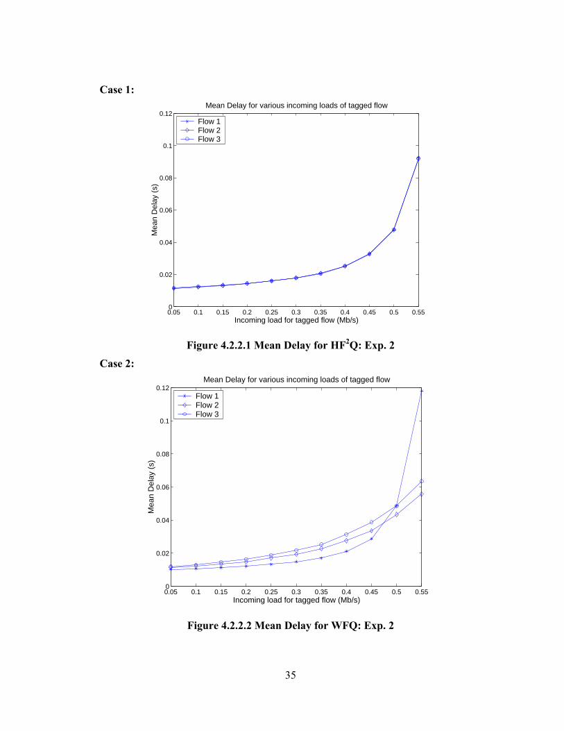
FIGURE 4.2.2.1 MEAN DELAY FOR HF2Q: EXP. 2 ........................................................ 35
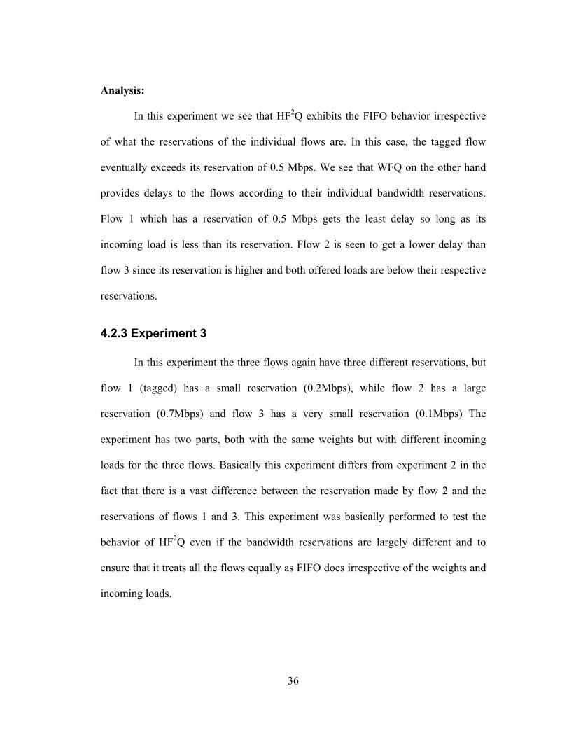
FIGURE 4.2.2.2 MEAN DELAY FOR WFQ: EXP. 2 ........................................................ 35
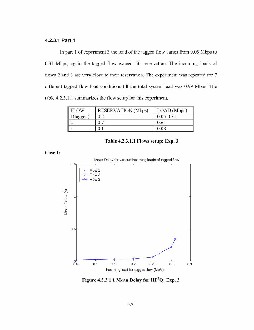
FIGURE 4.2.3.1.1 MEAN DELAY FOR HF2Q: EXP. 3 ..................................................... 37
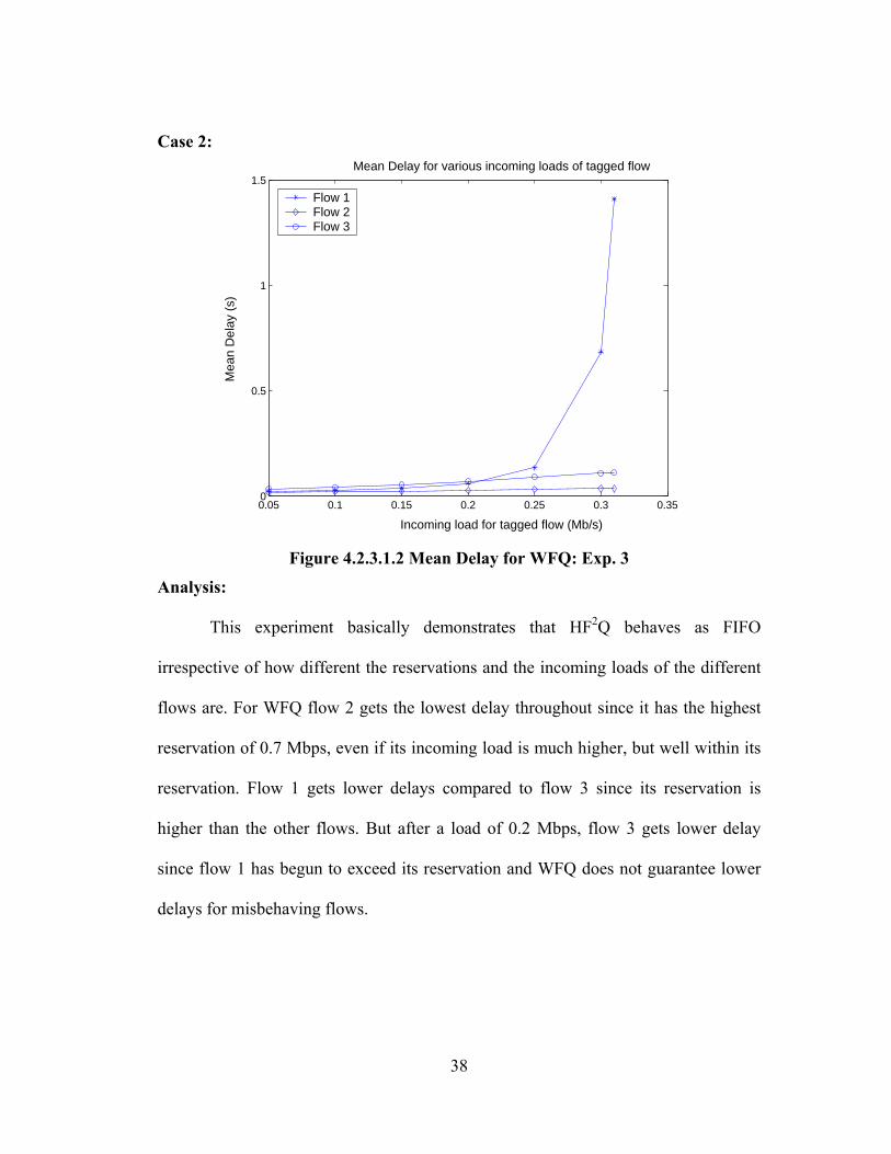
FIGURE 4.2.3.1.2 MEAN DELAY FOR WFQ: EXP. 3 ..................................................... 38
FIGURE 4.2.3.2.1 MEAN DELAY FOR HF2Q: EXP. 3 ..................................................... 39
FIGURE 4.2.3.2.2 MEAN DELAY FOR WFQ: EXP. 3 ..................................................... 40
FIGURE 4.3.1.1 MEAN DELAY FOR HF2Q: EXP. 1 ........................................................ 42
FIGURE 4.3.1.2 MEAN DELAY FOR WFQ: EXP. 1 ........................................................ 43
FIGURE 4.3.1.3 MEAN DELAY FOR HF2Q: EXP. 1 ........................................................ 43
FIGURE 4.3.1.4 MEAN DELAY FOR WFQ: EXP. 1 ........................................................ 44
FIGURE 4.3.2.1 MEAN DELAY FOR HF2Q: EXP. 2 ........................................................ 45
FIGURE 4.3.2.2 MEAN DELAY FOR WFQ: EXP. 2 ........................................................ 46
FIGURE 4.3.2.3 MEAN DELAY FOR HF2Q: EXP. 2 ........................................................ 46
FIGURE 4.3.2.4 MEAN DELAY FOR WFQ: EXP. 2 ........................................................ 47
FIGURE 4.3.3.1.1 MEAN DELAY FOR HF2Q: EXP. 3 ..................................................... 48
FIGURE 4.3.3.1.2 MEAN DELAY FOR WFQ: EXP. 3 ..................................................... 49
FIGURE 4.3.3.1.3 MEAN DELAY FOR HF2Q: EXP. 3 ..................................................... 49
FIGURE 4.3.3.1.4 MEAN DELAY FOR WFQ: EXP. 3 ..................................................... 50
FIGURE 4.3.3.2.1 MEAN DELAY FOR HF2Q: EXP. 3 ..................................................... 51
FIGURE 4.3.3.2.2 MEAN DELAY FOR WFQ: EXP. 3 ..................................................... 52
FIGURE 4.3.3.2.3 MEAN DELAY FOR HF2Q: EXP. 3 ..................................................... 52
FIGURE 4.3.3.2.4 MEAN DELAY FOR WFQ.................................................................. 53
FIGURE 4.4.1.1 THROUGHPUT FOR HF2Q: EXP. 1 ........................................................ 55
ix
FIGURE 4.4.1.2 THROUGHPUT FOR WFQ: EXP. 1......................................................... 55
FIGURE 4.4.1.3 THROUGHPUT FOR FIFO: EXP. 1......................................................... 56
FIGURE 4.4.2.1 THROUGHPUT FOR HF2Q: EXP. 2 ........................................................ 58
FIGURE 4.4.2.2 THROUGHPUT FOR WFQ: EXP. 2........................................................ 58
FIGURE 4.4.2.3 THROUGHPUT FOR FIFO: EXP. 2......................................................... 59
FIGURE 5.1.3.1 ALLOCATION MAP STRUCTURE ......................................................... 66
FIGURE 5.3.4.1 STATE DIAGRAM OF REQUEST/GRANT PROCESS ................................. 76
FIGURE 5.5.1 SIMULATION SCENARIO IN OPNET........................................................ 79
FIGURE 5.6.2.1 COMPARISON OF UGS AND BE DELAYS ............................................. 84
FIGURE 5.6.3.1 EFFECT OF FRAGMENTATION & CONCATENATION.............................. 87
FIGURE 5.6.4.2 EFFECT OF BACK-OFF ON COLLISION PROBABILITY (PIGGYBACKING
ENABLED) ............................................................................................................ 92
FIGURE 5.6.4.3 EFFECT OF BACK-OFF ON DELAY (PIGGYBACKING ENABLED)............. 93
FIGURE 5.6.5.1 EFFECT OF PIGGYBACKING ON COLLISION PROBABILITY .................... 95
FIGURE 5.6.5.2 EFFECT OF BACK-OFF ON DELAY (PIGGYBACKING ENABLED)............ 96
FIGURE 5.6.6.1 EFFECT OF PRIORITIES ON DELAY ....................................................... 99
FIGURE A1.1 MEAN DELAY FOR HF2Q: EXP. A......................................................... 107
FIGURE A1.2 MEAN DELAY FOR WFQ: EXP. A ......................................................... 108
FIGURE A1.4 MEAN DELAY FOR WFQ: EXP. A ......................................................... 109
FIGURE A1.6 MEAN DELAY FOR WFQ: EXP. A ......................................................... 110
FIGURE A1.10 MEAN DELAY FOR WFQ: EXP. B ....................................................... 112
x
LIST OF TABLES TABLE 4.2.1.1 FLOWS SETUP: EXP. 1........................................................................... 32
TABLE 4.2.2.1 FLOWS SETUP: EXP. 2........................................................................... 34
TABLE 4.2.3.1.1 FLOWS SETUP: EXP. 3........................................................................ 37
TABLE 4.2.3.2.1 FLOWS SETUP: EXP. 3........................................................................ 39
TABLE 4.3.1.1 FLOWS SETUP: EXP. 1........................................................................... 42
TABLE 4.3.2.1 FLOWS SETUP: EXP. 2........................................................................... 45
TABLE 4.3.3.1.1 FLOWS SETUP: EXP. 3........................................................................ 48
TABLE 4.3.3.2.1 FLOWS SETUP: EXP. 3........................................................................ 51
TABLE 4.4.1.1 FLOWS SETUP: EXP. 1........................................................................... 54
TABLE 4.4.2.1 FLOWS SETUP: EXP. 2........................................................................... 57
TABLE 4.5.1 QUANTIFICATION OF TRANSITIONAL BEHAVIOR OF HF2Q........................ 62
TABLE A1.1 FLOWS SETUP: EXP. A............................................................................ 107
TABLE A1.2 FLOWS SETUP: EXP. B............................................................................ 110
1
1 Introduction and Motivation
In the future, broadband networks will be an integral part of the global
communication infrastructure. With the rapid growth in popularity of wireless data
services and the increasing demand for multimedia multi-service applications (voice,
video, audio, data) it is expected that future broadband networks, both wired and
wireless, will provide services for heterogeneous classes of traffic with different
quality of service (QoS) requirements. Currently, there is an urgent need to develop
new technologies for providing QoS differentiation and guarantees in such networks.
Among all the technical issues that need to be resolved, packet scheduling is one of
the most important. Scheduling algorithms provide mechanisms for bandwidth
control, and congestion control policies are all dependent on the specific scheduling
algorithm used. Many scheduling algorithms capable of providing certain guaranteed
QoS have been developed for wireline networks.
The focus of this thesis is two-fold. The main focus is to characterize the
performance of a new scheduling algorithm called Hybrid FIFO Fair Queuing
(HF2Q). This new algorithm was stumbled upon by a fellow student [1] while
studying the properties of Weighted Fair Queuing, an existing queuing algorithm for
packet-switched networks. HF2Q has very interesting properties in that it is a
combination of two existing queuing schemes, namely the conventional First-In-First-
Out (FIFO) queuing scheme and WFQ. Detailed descriptions of all these are provided
in the subsequent chapters. Doing a complete performance characterization is
2
important since it helps us understand the operation and employ it in suitable
networks where such a behavior would be beneficial.
The other aspect of this thesis is to study the performance of IEEE 802.16
standard (standardized in 2001), which is the Medium Access Control standard for
wireless Metropolitan Area Networks (MAN) or fixed Broadband Wireless Access
(BWA) networks. IEEE 802.16 was largely based on Data Over Cable Service
Interface Specification 1.1 (DOCSIS 1.1), which is the defacto standard for delivering
broadband services over Hybrid Fiber Coax (HFC) networks. Hence the basic
protocol operation and QoS features of both the protocols are the same. IEEE 802.16
specifies a number of new features for providing QoS guarantees over a broadband
wireless network. It is important to understand the basic operation and the various
QoS features provided by this complex standard. This in turn helps in design of
wireless access systems with required QoS guarantees for specific end-users.
QoS and Scheduling
Many future applications of computer networks will rely on the ability of the
network to provide ``Quality of Service'' (QoS) guarantees. These guarantees are
usually in the form of bounds on end-to-end delay, bandwidth, delay jitter (variation
in delay), packet loss rate, or a combination of these parameters. Broadband packet
networks are currently enabling the integration of traffic with a wide range of
characteristics -- from video traffic with stringent QoS requirements to ``best-effort''
data requiring no guarantees – all within a single communication network. QoS
3
guarantees can also be provided in conventional IP packet networks by the use of
proper packet scheduling algorithms in the routers (gateways).
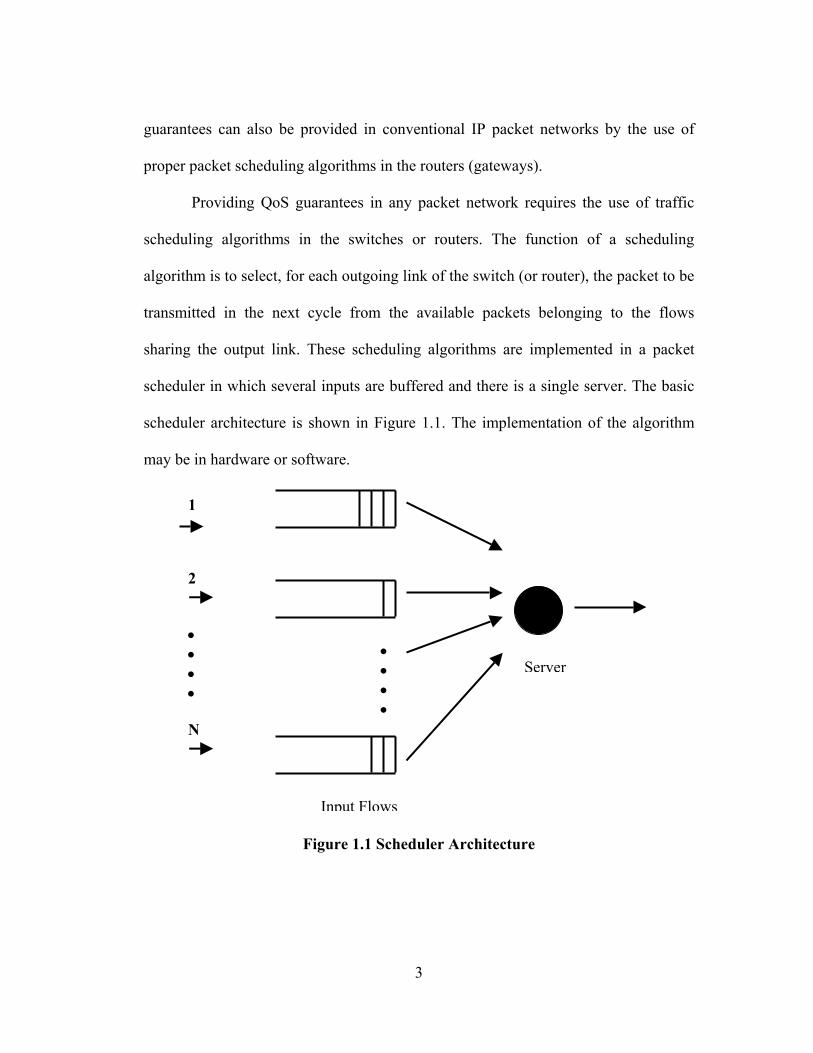
Providing QoS guarantees in any packet network requires the use of traffic
scheduling algorithms in the switches or routers. The function of a scheduling
algorithm is to select, for each outgoing link of the switch (or router), the packet to be
transmitted in the next cycle from the available packets belonging to the flows
sharing the output link. These scheduling algorithms are implemented in a packet
scheduler in which several inputs are buffered and there is a single server. The basic
scheduler architecture is shown in Figure 1.1. The implementation of the algorithm
may be in hardware or software.
Figure 1.1 Scheduler Architecture
Input Flows
• • • •
1 2
• • • • N
Server
4
Although it is possible to build a guaranteed performance service [2] on a
broad class of service disciplines, it is desired that a service discipline to be efficient,
protective, flexible, simple and fair.
Efficiency. To guarantee certain performance requirements we need a connection
admission control policy to limit the guaranteed service traffic load in the network. A
service discipline is more efficient than another one if it can meet the same end-to-
end performance guarantees under heavier load of guaranteed service traffic.
Protection. Guaranteed service requires that a network protects well-behaving
guaranteed service clients from three sources of variability: ill-behaving users,
network load fluctuation and best-effort traffic. It is essential that the service
discipline should meet the performance requirements of packets from well-behaving
guaranteed service clients even in the presence of ill-behaving users, network load
fluctuation and unconstrained best-effort traffic.
Flexibility. The guaranteed performance service needs to support applications with
diverse traffic characteristics and performance requirements. Because of the vast
diversity of traffic characteristics and performance requirements of existing
applications, as well as the uncertainty about future applications, an ideal service
discipline should be flexible to allocate different delay, bandwidth and loss rate
quantities to different guaranteed service connections.
Simplicity. The service discipline should be both conceptually simple to allow
tractable analysis and mechanically simple to allow high-speed implementation.
5
Fairness. Fairness is a desirable property in queuing algorithms that enable adequate
congestion control in networks even in the presence of ill-behaved sources (sources
that transmit at a rate more than what it is supposed to transmit at). Thus fairness in
the sense of allocating bandwidth and buffer space in a fair manner automatically
ensures that ill-behaved sources get no more than their fair share. WFQ provides this
sort of protection in the form of bandwidth allocation. But the concept of fairness can
also be viewed from a different perspective. While WFQ provides fair bandwidth
allocation, FIFO provides fairness in the sense that it provides equal mean waiting
time for packets from all flows irrespective of their offered load. In a sense, FIFO can
be deemed as a fair queuing scheme in that it does not discriminate between various
packets in terms of mean delay. Furthermore with FIFO queuing the order of arrival
determines the bandwidth and buffer allocation. The remainder of this thesis is
organized as follows.
Chapter 2 discusses the relevant work in the area of packet service disciplines
and IEEE 802.16 in the context of BWA networks.
Chapter 3 discusses Weighted Fair Queuing [WFQ] and the proposed
modification to it, resulting in a new queuing discipline Hybrid FIFO Fair Queuing
(HF2Q). Chapter 3 discusses the operation and features of HF2Q in detail.
Chapter 4 presents the analysis and results of the performance characterization
of HF2Q.
Chapter 5 presents a detailed discussion on the operation and performance
analysis of QoS aspects of IEEE 802.16 for Broadband Wireless Access networks.

6
Chapter 6 presents a summary of results obtained, conclusions drawn and
possible future work.
7
2 Background and Related Work
A number of service disciplines have been proposed in the past in the context
of high-speed packet switched network. The performances of these service disciplines
have been studied and new analysis techniques have been proposed to address their
performance issues. Since the one focus of this thesis is to discuss the performance of
a new service discipline as a modification of Weighted Fair Queuing, relevant work
in the area of queuing algorithms will be presented.
2.1 Classes of Queuing Algorithms
Queuing algorithms can be thought of as allocating three nearly independent
quantities [3]: bandwidth (which packets get transmitted), promptness (when do those
packets get transmitted), and buffer space (which packets are discarded by the
gateway). Multiple packets exist in one or more buffers sharing a common outgoing
link; the scheduler chooses a packet for service. There are several queuing methods,
including FIFO (first-in, first out), priority queuing, and fair queuing. All the queuing
algorithms discussed below are work conserving, that is, the server is never idle when
a packet is buffered in the system
1. FIFO queuing
The simplest queuing algorithm is the first-in, first-out queuing technique in
which the first packet in the queue is the first packet that is processed i.e. transmitted.
When the queue becomes full due to traffic congestion, incoming packets are
dropped. FIFO relies on end systems to control congestion via congestion control
8
mechanisms. FIFO queuing essentially relegates all congestion control to the sources,
since the order of arrival completely determines the bandwidth, promptness and
buffer space allocations. It thus does not offer any protection and it is not very
flexible in the sense that it does not provide performance guarantees for different
kinds of traffic. FIFO is extremely simple to implement and has a fairly tractable
analysis.
2. Priority queuing
This technique uses multiple queues, but queues are serviced with different
levels of priority, with the highest priority queues being serviced first. When
congestion occurs, packets tend to be dropped from lower-priority queues first. The
only problem with this method is that lower-priority queues may not get serviced at
all if high-priority traffic is excessive. Packets are classified and placed into queues
according to information in the packets, such as flow ID, explicit priority,
class/service indication, etc. Priority queuing is efficient in the sense that it provides
some amount of performance guarantees, i.e. gives preferential treatment to higher
priority queues compared to lower priority ones. It is also easy to implement.
3. Fair queuing
The fair queuing concept was originally proposed by Nagle [4] in order to
solve the problem of malicious or erratic TCP implementations. The goal of the
algorithm was to guarantee each session a portion of the network resources even
though some sessions are transmitting at a higher rate than the allocated one. A
9
round-robin approach is used to service all queues in a fair way. This prevents any
one source from overusing its share of network capacity. Fair Queuing service
disciplines address this scheduling problem by allocating bandwidth fairly among
competing flows regardless of their prior usage or congestion. In particular, these
disciplines do not penalize flows for the use of idle bandwidth. Fairness offers
protection from “misbehaving” flows and leads to effective congestion control and
better services for rate-adaptive applications. Strict QoS guarantees such as
throughput or delays can also achieved. Some of the important work related to fair
queuing is described below.
A. Virtual Clock
The Virtual clock discipline [5] aims to emulate the Time Division
Multiplexing (TDM) scheme. Each packet is allocated a virtual transmission time,
which is the tine at which the packet would have been transmitted were the server
actually doing TDM. The packets are transmitted in the increasing order of virtual
transmission times. Virtual Clock algorithm ensures that a well-behaving
connection gets good performance in the presence of connections that send
packets at a rate higher than they are supposed to.
B. WFQ and WF2Q
Weighted Fair Queuing (WFQ) [3] is a packet scheduling policy that tries to
approximate Fluid Fair Queuing (FFQ) or Generalized Processor Sharing (GPS)
policy [6]. FFQ is a general form of head-of-line processor sharing service
discipline [7]. There is a separate FIFO queue for each connection sharing the
10
same link. GPS serves the non-empty queues in proportion to their service shares.
GPS is impractical since it assumes that the server can serve all connections with
non-empty queues simultaneously and the traffic is infinitely divisible. WFQ, also
known as the Packet Generalized Processor Sharing or PGPS [8], is the most well
known approximation of the GPS service in a packet system. In WFQ when the
server is ready to transmit the next packet at a particular time t, it picks the first
packet that would complete service in the corresponding GPS system if no
additional packets were to arrive after t.
While WFQ uses only finish times of packets in the GPS system, WF2Q [9]
(Worst Case Weighted Fair Queuing) uses both start times and finish times of the
packets in the GPS system to achieve a more accurate emulation. In WF2Q, when
the next packet is chosen for service at time t, rather than selecting it from among
all the packets at the server as in WFQ, the server only considers the set of
packets that have started receiving service in the corresponding GPS system, and
selects the packet among them that would complete service first in the
corresponding GPS system.
WFQ and WF2Q have most of the properties desired in a queuing algorithm.
They offer protection to well-behaving flows under overloaded conditions and
they are very flexible in the sense that they can support applications with different
performance requirements. The main drawback is that it is not very easy to
implement.
11
C. Self-Clocked Fair Queuing A simpler packet approximation algorithm of GPS is Self-Clocked Fair
Queuing (SCFQ) [10] also known informally as “Chuck’s Approximation” [11].
To reduce the complexity in computing the reference times in the GPS system,
SCFQ introduces an approximation algorithm based on the observation that the
system’s time in the reference GPS system at any moment may be estimated from
the service time of the packet currently being serviced. Moreover, SCFQ scheme
is nearly optimal in the sense that the services received by any pair of backlogged
sessions, normalized to the corresponding service shares, stay close to each other.
4. CBQ (Class-Based Queuing)
CBQ [12] is a class-based algorithm that schedules packets from several
queues and guarantees a certain transmission rate to each queue. If a queue is not in
use, the bandwidth is made available to other queues. From this simple description,
CBQ is seen to be similar to WFQ. But CBQ is a hierarchical queuing algorithm. In
hierarchical link sharing [13] there is a class hierarchy associated with each link that
specifies the resource allocation policy for that link. A class represents a traffic
stream or aggregate of traffic streams that are grouped according to administrative
affiliation, protocol, traffic type or other criteria. A CBQ-compliant device looks
within packets to classify packets according to addresses, application type, protocol,
URL, or other information. Thus CBQ is more than a queuing scheme; it is also a
QoS scheme that identifies different types of traffic and queues the traffic according
to predefined parameters.
12
5. Delay-Earliest-Due-Date (Delay-EDD)
Delay-EDD [14] is an extension to the classic Earliest-Due-Date-First
scheduling [15], in which each packet from a periodic traffic stream is assigned a
deadline and the packets are sent in the order of increasing deadlines. In Delay-EDD,
the server negotiates a contract with each source wherein if a source obeys its
promised traffic specification, then the server will provide a delay bound. The key
lies in the assignment of deadlines to packets. The server sets a packet’s deadline to
the time at which it should be sent had it been received according to the contract.
2.2 MAC Standard for Fixed Broadband Wireless Access
Broadband Wireless Access (BWA) systems have gained an increased interest
during the last two years. This has been fuelled by a large demand on high frequency
utilization resulting in a crowded spectrum as well as a large number of users
requiring simultaneous multi-dimensional high data rate. A BWA system uses new
network architectures to deliver broadband services in a fixed point-to-point or point-
to-multipoint configuration to residential and business customers. BWA networks
support voice, data, video distribution services and emerging interactive multimedia
communications. Large bandwidth, lower installation cost and ease of deployment,
coupled with recent advancements in semiconductor technologies for wireless
applications, make BWA an attractive solution for broadband service delivery. The
wireless medium is a shared medium, which demands a Medium Access Control
(MAC) protocol to co-ordinate the transmission of multiple traffic flows over it. The
downlink flows are simply multiplexed by the access point and there is no contention.
13
The uplink direction is more challenging because of potential contention, and the
MAC protocol is needed to minimize the contention probability. The medium access
control protocol also has to include the uplink scheduling in order to accommodate
the demand assignment multiple access and dynamic resources allocation. The IEEE
802.16 standard [16] has formally been approved as the standard for BWA networks
by the IEEE Standards Association in 2001. It is worth mentioning that IEEE 802.16
is a consolidation of two proposals, one of which was based on Data Over Cable
Service Interface Specification (DOCSIS) [17]. DOCSIS is the de facto standard for
delivering broadband services over Hybrid Fiber Coax (HFC) cable networks.
DOCSIS was developed by a group of major cable operators called Cable Labs.
DOCSIS was later adopted by the ITU and is now supported by many vendors.
Versions 1.0 and 1.1 of DOCSIS were introduced in 1999, and version 2.0 was
introduced in 2000.
Not much relevant work has been done directly in the area of performance
analysis of Medium Access Control standard (IEEE 802.16) for BWA. [18] discusses
the performance of possible MAC protocols for Fixed Broadband Wireless Access
Networks. [19] describes new Quality of Service Scheduling architecture for Cable
and BWA systems.

14
3 Description of HF2Q Hybrid FIFO Fair Queuing (HF2Q) is a new service discipline for packet-
switched networks that exhibits the properties of both WFQ and First In First Out
(FIFO) under different load conditions. This new behavior is a result of a
modification in the operation of regular WFQ. This chapter presents a detailed
description of the notion of FIFO in comparison with fair queuing, the evolution of
WFQ and its principles of operation, a description of HF2Q operation and its
interesting properties, and a summary of comparison of both the service disciplines.
3.1 First In First Out (FIFO)
First-Come-First-Serve (FCFS) or First-In-First-Out (FIFO) is one of the
simplest scheduling policies. Its operation is that packets are served in the order in
which they are received. It is quite simple to implement. In particular, insertion and
deletion from the queue of the waiting packets are constant time operations and do
not require any per-connection state to be maintained by the scheduler, so it is one of
the most commonly implemented policies. However, the “best-effort service “ offered
by FIFO scheduling does not readily provide delay or throughput guarantees.
In terms of delay, FIFO results in the same expected waiting time for every
arriving packet (at least under the assumption of Poisson arrivals). FIFO provides no
mechanism for providing different waiting times for different flows. In some sense,
this is “fair” treatment of the flows. One way to provide a delay bound (for all flows)
is to limit the buffer size so that once a packet is queued up for transmission it is
15
guaranteed to be sent out in the time it takes to serve a full queue of packets. But in
this case, packets have to be dropped if the limited buffer is full when packets arrive.
Neither does FIFO explicitly provide any mechanisms for fair sharing of link
resources, but with the help of some buffer management schemes it is possible to
control the sharing of bandwidth. Buffer management schemes [20] can be achieved
by monitoring the congestion levels of queues (queue occupancy or queue occupancy
increase rate) and using this mechanism to modify buffer portioning or discarding
policy. FIFO does not provide flow isolation and essentially relegates all congestion
control to the sources, since the order of arrival completely determines the bandwidth
promptness and buffer allocations. So there have to be flow control algorithms which
when universally implemented can overcome these limitations. Unfortunately, no
matter what congestion control is used at the sources, FIFO does not protect well-
behaved sources against ill-behaved ones. A single source sending packets at a
sufficiently high speed can capture a high fraction of bandwidth of the outgoing line
[3]. As mentioned before, for a finite buffer case the delay is then very high but is
bounded, but for an infinite buffer the delay of all the packets grows infinitely.
3.2 Fair Queuing Criterion
Fair queuing was originally developed [4] as an attempt to maintain fairness in
the amount of services provided at a service point to the competing users. Unlike
FIFO queuing discipline where a session can increase its share of service by
presenting more demand and keeping a large number of packets in the queue, the
primary goal in fair queuing is to serve sessions in proportion to some pre-specified
16
service shares, independent of queuing load presented by the sessions. Fair queuing
algorithms provide protection, so that ill-behaved flows have only limited negative
impact on well-behaved flows. Allocating bandwidth and buffer space in a fair
manner automatically ensures that ill-behaved sources can get no more than their fair
share.
A queuing algorithm is said to be fair if the fairness criterion holds. We begin
by introducing some notations. Consider a queuing system served by an access link
with a total output link capacity of C (bits/second). Let us denote by K the set of
flows setup on this link, and by rk, Kk ∈ , the service rate (in bits/second) associated
with each flow k. Define Wk(t1, t2), t2 > t1, as the aggregate service (in bits) received
by flow k during the time interval [t1, t2]. The value of Wk(t1, t2) is simply equal to the
time spent by the server on flow k during [t1, t2] times the server speed C. Wk(t1, t2) /
rk is then the total service provided to flow k during the time interval [t1, t2]
normalized to its corresponding transmission rate. We call this quantity the
normalized service received by k during [t1, t2]. At any time t, a flow may be
backlogged or else absent. A flow is backlogged at time t if a positive amount of
session’s traffic is queued at time t. We denote by B(t) the set of flows that are
backlogged at time t and by B (t1, t2) the set of flows that are backlogged during the
entire interval [t1, t2]. The fairness criterion is said to hold if the following condition
is satisfied:
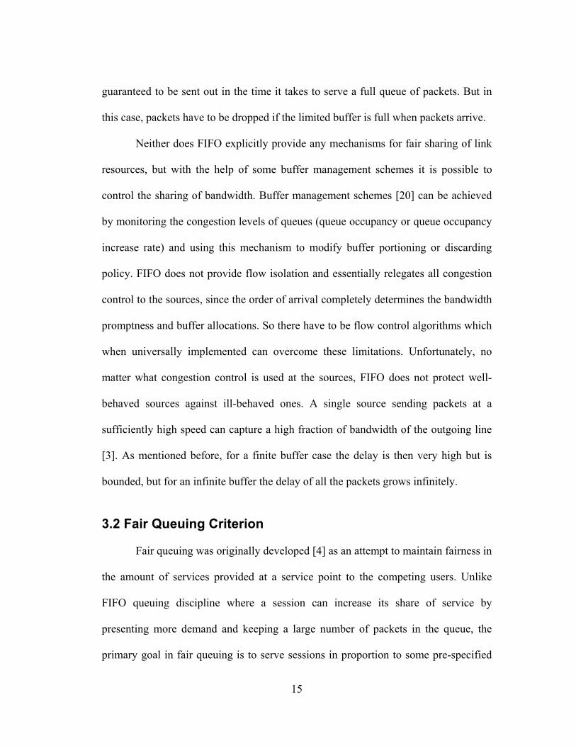
For intervals of time [t1, t2], in which both the flows k and j are backlogged,
17
),(,,0),(),(
212121 ttBkj
rttW
rttW
j
j
k
k ∈=− (3.2.1)
In real packet networks, an entire packet of a certain flow must be transmitted before
service may be shifted to another flow. Therefore, it is not possible to satisfy the
fairness criterion above exactly for all intervals of time. Instead, the objective of a fair
packet-scheduling algorithm is to ensure that the quantity |/),(/),(| 2121 jjkk rttWrttW −
is bounded for all intervals of time and is as close to zero as possible.
3.2.1 Generalized processor Sharing
Generalized-Processor-Sharing (GPS) is an ideal scheduling discipline that is
defined with respect to a fluid-model, where packets are considered to be infinitely
divisible. Thus it is also called as Fluid Fair Queuing (FFQ) [2]. With a fluid flow
model of traffic, the service is offered to sessions in arbitrarily small increments.
Equivalently, it may be assumed that multiple sessions can receive service in parallel.
As a result, it is possible to divide the service among the sessions, at all times, exactly
in proportion to the specified service shares. A GPS server is work conserving and
operates at a fixed rate C. It is characterized by positive real numbers r1, r2,
r3,…………..rN. Let Wk(t1, t2) and Wj(t1, t2), be defined as before , then a GPS server is one
which
Njrr
ttWttW
j
k
j
k ...,3,2,1,),(),(
21
21 =≥ (3.2.1.1)
for any session k that is continuously backlogged in the interval [t1,t2].
Session k is guaranteed a rate of
18
Cr
rg
jj
kk ∑
= (3.2.1.2)
A problem with GPS is that it is an idealized discipline that does not transmit packets
as entities. It assumes that the server can serve multiple sessions simultaneously and
that traffic in infinitely divisible. But in actual packet-based traffic scenarios, only
one session can receive service at a time, and an entire unit of traffic (referred to as a
packet) must be served before another unit is picked up for service.
3.3 Weighted Fair Queuing
Weighted Fair Queuing (WFQ) and its derived algorithms are excellent
approximations to the more generalized and ideal form of fair queuing viz,
Generalized Processor Sharing (GPS) even when the packets are of variable length.
Round Robin, which is an early form of fair queuing, assumes an equal service share
for all the sessions and an equal length for all packets. It provides service to the
sessions in a round robin fashion, picking one packet for service from each session
(or queue) with backlogged traffic, and then proceeding to the next session. When the
lengths of the packets are not the same and/or the service shares assigned to the
sessions are not equal, the definition of fair queuing and the right order of providing
service becomes a more subtle matter. To formulate fair queuing in this more general
case, the notion of fairness was applied to an idealized fluid-flow traffic environment
and then the outcome was used to specify fair queuing for the actual packet-based
traffic scenario. Packet-by-Packet GPS (PGPS) or WFQ does not make the
19
infinitesimal packet size assumption in GPS, and with variable-size packets, they do
not need to know a connection's mean packet size in advance.
3.3.1 Transmission Scheme Let Fp be the time at which packet p will depart (finish service) under GPS.
Then, a very good approximation of GPS would be a work-conserving scheme that
serves packets in increasing order of Fp. Now suppose the server becomes idle
(completes service of some packet) at time t. The next packet to depart under GPS
may not have arrived at time t and, since the server has no knowledge of when this
packet will arrive, there is no way for the server to be both work conserving and serve
the packet in increasing order of Fp. The server picks the first packet that would
complete service under the GPS simulation if no additional packets were to arrive
after time t. This scheme is accomplished as follows.
3.3.2 Virtual time WFQ operation is linked to the reference fluid-based GPS system by defining
a system-wide function called virtual time. The virtual time, denoted by v(t), is
associated with the reference GPS system and measures the progress of work in that
system; it is dependent on system load. The virtual time is used in WFQ to define the
order in which packets are served in the packet-by-packet scheduling algorithm. The
definition of the virtual time is that v(t) has a rate of increase in time equal to that of
the normalized service received by any backlogged flow k in the reference GPS
20
system. In the reference fluid-based system, all backlogged flows receive exactly the
same normalized service with time. Mathematically,
( ) ( )
),(,.
,0lim)( tttBk
rttWtttW
ttvdtd
k
kk ∆+∈
∆
−∆+→∆≡ (3.3.2.1)
In other words, during a busy period of the server, we can say that:
),(,),(
)()( 2121
12 ttBkr
ttWtvtv
k
k ∈=− (3.3.2.2)
where [t1, t2] is an arbitrary subinterval of the busy period. It can be shown that the
above definition leads to the following expression for evaluating v(t):
)()()( 12
),(
12
21
ttr
Ctvtv
ttBkk
−⋅=−∑
∈
(3.3.2.3)
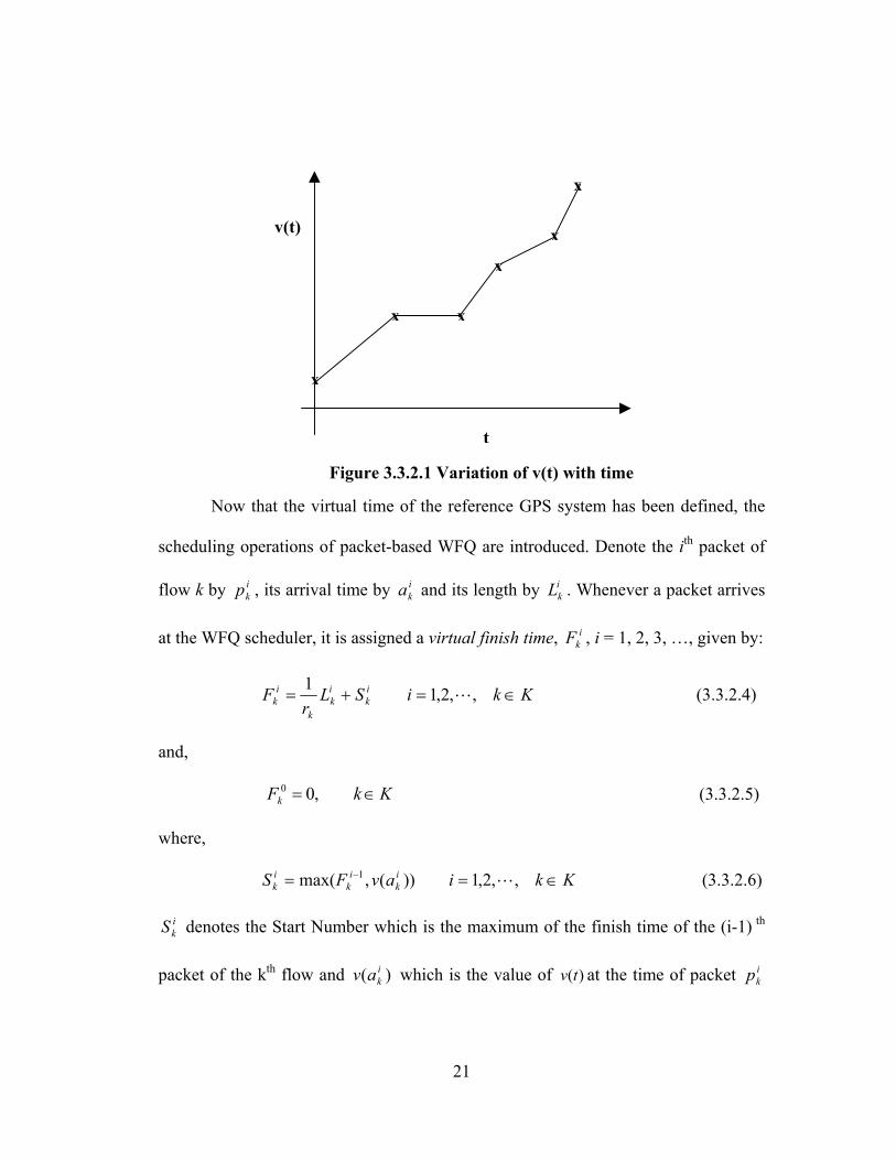
where C is the total output link capacity in bits/s. Hence, v(t) is a piecewise linear
increasing function of time with a slope that changes whenever the set of backlogged
flows B(t) changes and is inversely proportional to the sum of service shares of
sessions backlogged. Figure 3.3.2.1 shows the variation of v(t) with time. Note that
v(t) does not in general have a monotonically increasing slope (as illustrated in the
figure).
21
Now that the virtual time of the reference GPS system has been defined, the
scheduling operations of packet-based WFQ are introduced. Denote the ith packet of
flow k by ikp , its arrival time by i
ka and its length by ikL . Whenever a packet arrives
at the WFQ scheduler, it is assigned a virtual finish time, ikF , i = 1, 2, 3, …, given by:
KkiSLr
F ik
ik
k
ik ∈=+= ,,2,11
L (3.3.2.4)
and,
KkFk ∈= ,00 (3.3.2.5)
where,
KkiavFS ik
ik
ik ∈== − ,,2,1))(,max( 1 L (3.3.2.6)
ikS denotes the Start Number which is the maximum of the finish time of the (i-1) th
packet of the kth flow and )( ikav which is the value of )(tv at the time of packet i
kp
x
x
x
x
x
x
v(t)
t
Figure 3.3.2.1 Variation of v(t) with time
22
arrival. If the packet arrival is to an inactive queue, then the start number would be
the current virtual time (i.e. )( ikav ). If the arrival is to an active queue, then the start
number would be the finish time of the last packet in the queue on arrival. It can be
shown [2] that serving packets in the order of increasing virtual finish times ikF , as
computed by (3.3.2.4) and (3.3.2.5), is equivalent to serving them in the increasing
order of their actual finish times in the reference GPS system. Hence, all WFQ has to
do is compute a virtual finish time tag for each arriving packet and then serve packets
in the increasing order of their virtual finish time tags. Computing finish time tags for
each arriving packet is a simple operation that requires knowing only the packet’s
length, virtual finish time of the previous packet, and the system’s virtual time when
the packet arrives. Some of properties of the virtual time interpretation from the
standpoint of implementation are
• The virtual finishing times can be determined at the packet arrival
time.
• The packets are served in the order of virtual finishing time.
• We need to update the virtual time when there are events in the GPS
system, where each arrival and departure from the GPS system is
denoted as an event.
However the price to be paid for these advantages is some overhead in
keeping track of the set of backlogged flows. Another troublesome point in the
implementation of WFQ, as outlined above, is the requirement of evaluating v(t) of
23
the reference GPS system at each packet arrival instant. As mentioned earlier, v(t) is a
piecewise linear function, the slope of which changes whenever some flow k becomes
backlogged or absent in the reference GPS system. Such slope changes constitute
breakpoints in the piecewise linear form of v(t).The computational complexity of
evaluating v(t) depends on the frequency of such breakpoints.
3.4 Hybrid FIFO Fair Queuing (HF2Q)
This promising new queuing algorithm was stumbled upon during the process
of development of new simulation module for WFQ [1]. It turns out that introducing a
minor modification to the operations of WFQ transforms such a fair queuing policy
into a totally different queuing algorithm that exhibits very interesting properties. We
now call the new algorithm the Hybrid-FIFO/FQ system (or HF2Q for short) because
it exhibits desirable properties from both WFQ and FIFO scheduling policies. It
exhibits fairness in both perspectives, i.e. in bandwidth allocation (protecting well-
behaved sources in an overloaded system as WFQ does) and also offering equal mean
waiting times to all flows (as FIFO does) when total offered load is less than unity.
The description of this new queuing algorithm is presented here and its properties and
behavior are investigated in the next chapter. The following sections describe the
modifications required to transform WFQ into HF2Q and explain the preliminary
observations made about this new queuing system.
24
3.4.1 Modifications made to formulate HF2Q The operations of packet-based FQ algorithms (including WFQ) explained in
previous sections are dependent on virtual time, v (t), which in WFQ is calculated
using (3.3.2.2)
)()()( 12
),(
12
21
ttr
Ctvtv
ttBkk
−⋅=−∑
∈
(3.4.1.1)
where C is the total output link capacity in bits/s and [t1, t2] is a of a busy
period of the associated reference GPS system subinterval in which the set of
backlogged flows B(t) does not change. Hence, v(t) is a piecewise linear increasing
function of time with a slope that changes whenever the set of backlogged flows B(t)
changes. When a packet arrives, virtual time (represented by a variable called
roundNumber in the actual implementation) is updated. The implementation keeps
track of instants of time when the roundNumber is updated using the
lastRUpdateTime variable, which indicates the last time when the roundNumber was
updated.
( ) capacityweightSum
eTimelastRUpdatecurrentTimrroundNumberroundNumbe ⋅−
+=
(3.4.1.2)
In HF2Q, the lastRUpdateTime variable is not updated in a scenario when the
roundNumber variable is not updated at a new packet arrival because there are no
backlogged flows in the reference GPS system, i.e. the GPS system is idle in an
interval [t, t1] and a packet arrives at instant t1. For WFQ, the lastRUpdateTime
25
variable has to be updated at every packet arrival irrespective of the queuing system
status.
3.4.2 Comparison of WFQ and HF2Q operations In WFQ, calculating the virtual time during a busy period is done using
(3.4.1.1), where the break points t1 and t2 are the instants of new arrivals and/or
departures as seen by the reference GPS system. The arrivals at the GPS system are
the same as those at the WFQ system. On the other hand, departure instants might be
different for both systems. Since both GPS and WFQ are work conserving disciplines,
their busy periods coincide, i.e., the GPS server is in a busy period if and only if the
WFQ server is in a busy period. Let eτ be the end of a busy period and at this time
updating v(t) should be stopped, which means it would remain at ( )ev τ . When a new
busy period starts again by a new arrival (say flow a1) at sτ , the first packet arrival is
processed based on ( ) ( )es vv ττ = . Let the next arrival be at time 2τ and assume that the
first packet has not completed service by 2τ . Then v(t) would be correspondingly
updated to
( ) )()( 2
),(
2
211
1
s
Baa
s rCvv ττττ
ττ
−⋅+=∑
∈
(3.4.2.1)
Calculating the virtual time in H-F2Q is exactly the same as in WFQ until the
end of a busy period. The virtual time function for HF2Q is denoted by v’(t) . At the
end of a busy period eτ , the value of the virtual time is maintained as ( )ev τ , but the
variable lastRUpdateTime is not updated. This means that at a new busy period, the
26
first arrival at sτ receives a time stamp based on ( ) ( )es vv ττ = exactly as in WFQ.
However, for the next (second) arrival at 2τ , v(t) would be updated to
( ) )()( 2
),(
2
211
1
e
Baa
s rCvv ττττ
ττ
−⋅+=∑
∈
(3.4.2.2)
rather than to the expression mentioned in (3.4.2.1). This means that the second
arrival gets a much bigger timestamp than it would under WFQ (i.e., is delayed more)
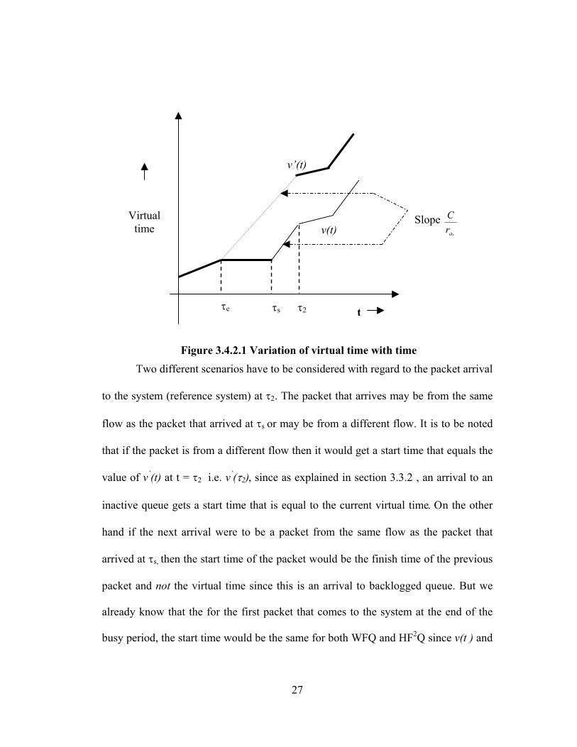
since (τ2−τe) is greater than (τ2−τs) as indicated in figure 3.4.2.1. Figure 3.4.2.1
illustrates the change of virtual time with time in both the queuing disciplines, i.e.
WFQ and HF2Q. v(t) for HF2Q is denoted as v’(t) and is shown in bold in the figure.
As can be seen in the figure, from time 2τ onward, the virtual time v’(t) is offset from
v(t) by a value of )(1
esarC ττ − due to the fact the lastRupdateTime variable was not
updated; that is, from 2τ onward both v(t) and v’(t) increase with the same slope. The
figure 3.4.2.1 assumes that the second packet is from a different flow than the first
packet, so that the slope of v(t) and also v’(t) changes at time 2τ .
27
Figure 3.4.2.1 Variation of virtual time with time
Two different scenarios have to be considered with regard to the packet arrival
to the system (reference system) at τ2. The packet that arrives may be from the same
flow as the packet that arrived at τs or may be from a different flow. It is to be noted
that if the packet is from a different flow then it would get a start time that equals the
value of v’(t) at t = τ2 i.e. v’(τ2), since as explained in section 3.3.2 , an arrival to an
inactive queue gets a start time that is equal to the current virtual time. Οn the other
hand if the next arrival were to be a packet from the same flow as the packet that
arrived at τs, then the start time of the packet would be the finish time of the previous
packet and not the virtual time since this is an arrival to backlogged queue. But we
already know that the for the first packet that comes to the system at the end of the
busy period, the start time would be the same for both WFQ and HF2Q since v(t ) and
Virtual time
tτs τ2 τe
v’(t)
v(t) Slope
1arC
28
v’(t) are the same at t= τs. In both the scenarios the packet ordering would eventually
be different than the packet ordering for normal WFQ. This has a cumulative effect
on the order of scheduling of future packets from the different flows. As we will see
in the next chapter, packets get ordered as in a FIFO queuing system if the system
load is less than unity. Of course, if the first packet already left the GPS system by 2τ ,
this means that we reached the end of another busy period.
3.4.3 Properties of HF2Q
Preliminary investigation of the HF2Q queuing system in chapter 4 indicates
that if the normalized system load is smaller than unity (i.e., 1≤ρ ), the queuing
system provides the same mean packet delay for all supported flows (similar to the
behavior of first-in first-out FIFO queuing). However, if the system load rate grows
beyond unity (i.e., when the system encounters a congestion period), the system
reverts back to operate as a WFQ system, providing protection against misbehaving
flows. In such mode, the mean packet delay of misbehaving flows (flows that send
above their capacity reservations) grows dramatically while the delay of other
behaving flows is kept finite, in the same way WFQ operates.
29
4 Simulations And Analysis of Results Simulations studies were conducted under various scenarios to characterize
the performance of HF2Q. The simulations were performed using the Extend
simulation software. Extend (Imagine That Inc.) is a simulation environment with
many features like model libraries, hierarchies of models, and its own modeling
language (ModL) which resembles C. It targets both continuous systems and discrete
event systems simulation, also offering the possibility of combining the two
paradigms. This research was conducted using discrete event simulation techniques.
4.1 Simulation Setup
Each experiment basically had a certain number of flows with each making its
own bandwidth reservation. Since the study was being done in a Broadband Wireless
Access context, a link speed of 1Mbps was chosen for all the experiments. Speeds in
wireless broadband can go from sub one megabit (< 1 Mbps) to 45 Mbps range. All
the flows transmitted packets whose lengths were uniformly distributed between
4000-12000 bits so that the mean packet length was 8000 bits. The arrival process for
each flow was Poisson. The simulations were run for an average of 2000 s. This
ensured that even for both low and high load cases more than 100,000 packets were
generated for a given run. In each simulation there were three flows (or sources), and
the incoming load of one of the flows was varied, keeping the loads of the other flows
constant. In all of the simulations, the flow (flow 1) whose load keeps varying is
named the tagged flow and the other flows are named non-tagged.
30
The aim of the different simulation experiments was to characterize the
performance of HF2Q in terms of two performance requirements, namely the average
delay and throughput. The average packet delay was measured for each flow for
varying incoming loads of the tagged flow. Throughput measurements were also
performed for certain cases. Each simulation was setup for a specified number of
runs wherein the incoming load of the tagged flow is different for each run and the
different flows had specified bandwidth reservations (indicated by weights). The aim
of the simulations was to characterize the performance of HF2Q in two scenarios:
When the total load of the system is less than 1
When the total load exceeds one (i.e. when the system is overloaded).
Also a comparison with WFQ is also shown for each of the different cases.
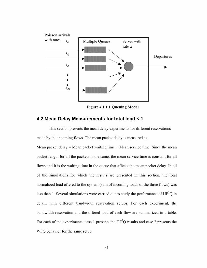
4.1.1 Queuing Model
A M/G/1 queuing model is considered, in which arrivals from flow 2
constitute a Poisson process with rate λi (exponential interarrival times) and service
times are independent, identically distributed with a general probability distribution
with mean service rate µ. In our case, the service times are uniformly distributed with
a mean of 8 ms. Figure 4.1.1.1 illustrates the queuing model. There are a total of N
queues and a single server to process packets from all of these queues. Each queue
has its own arrival rate (λ1,λ2,λ3,........λN).
31
Figure 4.1.1.1 Queuing Model
4.2 Mean Delay Measurements for total load < 1
This section presents the mean delay experiments for different reservations
made by the incoming flows. The mean packet delay is measured as
Mean packet delay = Mean packet waiting time + Mean service time. Since the mean
packet length for all the packets is the same, the mean service time is constant for all
flows and it is the waiting time in the queue that affects the mean packet delay. In all
of the simulations for which the results are presented in this section, the total
normalized load offered to the system (sum of incoming loads of the three flows) was
less than 1. Several simulations were carried out to study the performance of HF2Q in
detail, with different bandwidth reservation setups. For each experiment, the
bandwidth reservation and the offered load of each flow are summarized in a table.
For each of the experiments, case 1 presents the HF2Q results and case 2 presents the
WFQ behavior for the same setup
• • •
Multiple Queues Server with rate µ
Departures
Poisson arrivals with rates λ1
λ2
λ3
• • •
λN
32
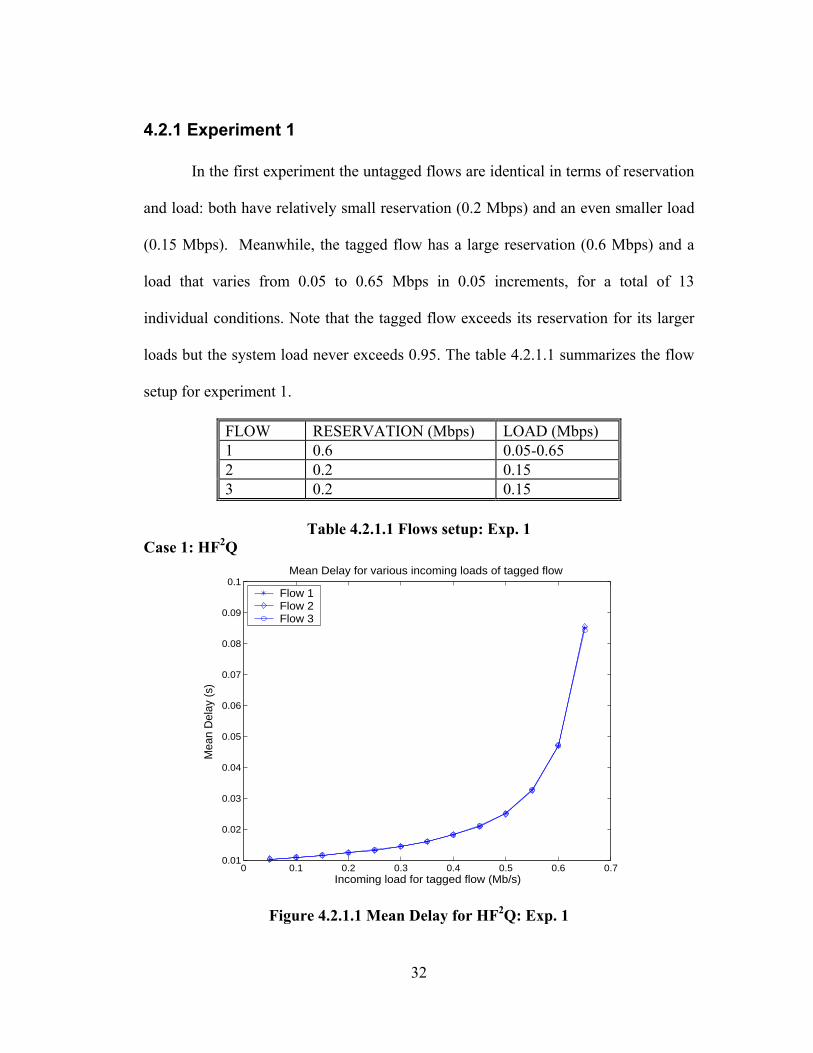
4.2.1 Experiment 1
In the first experiment the untagged flows are identical in terms of reservation
and load: both have relatively small reservation (0.2 Mbps) and an even smaller load
(0.15 Mbps). Meanwhile, the tagged flow has a large reservation (0.6 Mbps) and a
load that varies from 0.05 to 0.65 Mbps in 0.05 increments, for a total of 13
individual conditions. Note that the tagged flow exceeds its reservation for its larger
loads but the system load never exceeds 0.95. The table 4.2.1.1 summarizes the flow
setup for experiment 1.
FLOW RESERVATION (Mbps) LOAD (Mbps) 1 0.6 0.05-0.65 2 0.2 0.15 3 0.2 0.15
Table 4.2.1.1 Flows setup: Exp. 1
Case 1: HF2Q
0 0.1 0.2 0.3 0.4 0.5 0.6 0.70.01
0.02
0.03
0.04
0.05
0.06
0.07
0.08
0.09
0.1Mean Delay for various incoming loads of tagged flow
Incoming load for tagged flow (Mb/s)
Mea
n D
elay
(s)
Flow 1Flow 2Flow 3
Figure 4.2.1.1 Mean Delay for HF2Q: Exp. 1
33
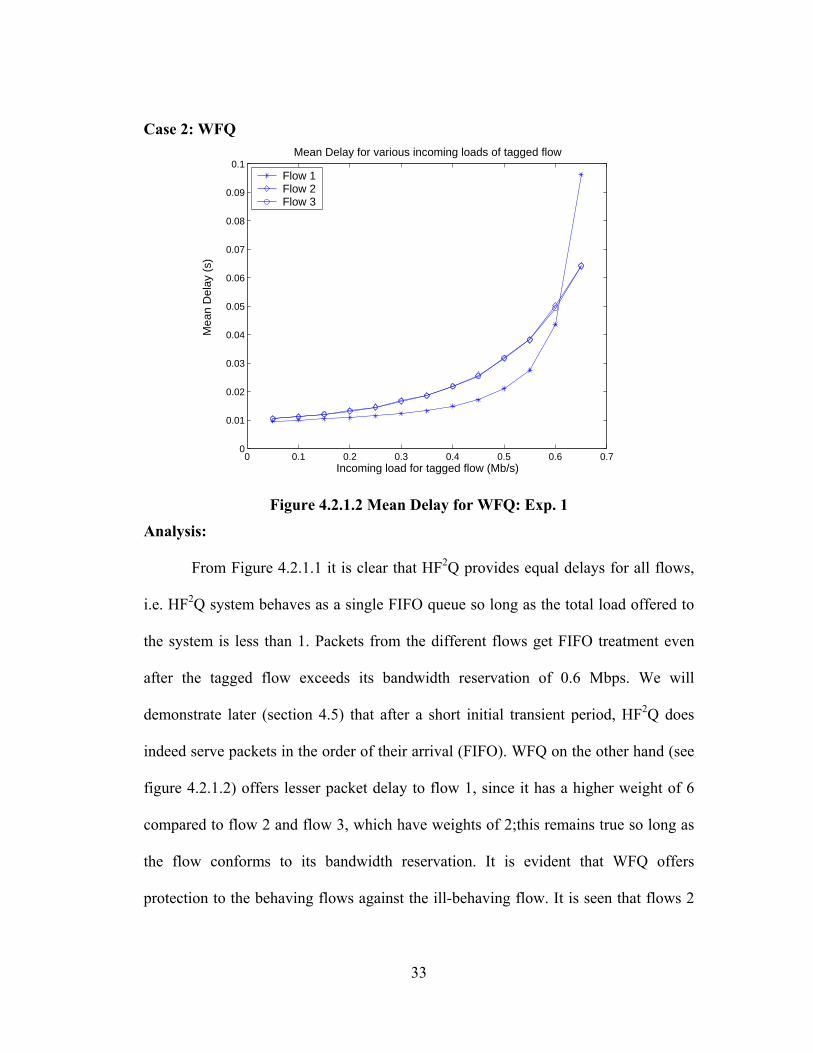
Case 2: WFQ
0 0.1 0.2 0.3 0.4 0.5 0.6 0.70
0.01
0.02
0.03
0.04
0.05
0.06
0.07
0.08
0.09
0.1Mean Delay for various incoming loads of tagged flow
Incoming load for tagged flow (Mb/s)
Mea
n D
elay
(s)
Flow 1Flow 2Flow 3
Figure 4.2.1.2 Mean Delay for WFQ: Exp. 1
Analysis:
From Figure 4.2.1.1 it is clear that HF2Q provides equal delays for all flows,
i.e. HF2Q system behaves as a single FIFO queue so long as the total load offered to
the system is less than 1. Packets from the different flows get FIFO treatment even
after the tagged flow exceeds its bandwidth reservation of 0.6 Mbps. We will
demonstrate later (section 4.5) that after a short initial transient period, HF2Q does
indeed serve packets in the order of their arrival (FIFO). WFQ on the other hand (see
figure 4.2.1.2) offers lesser packet delay to flow 1, since it has a higher weight of 6
compared to flow 2 and flow 3, which have weights of 2;this remains true so long as
the flow conforms to its bandwidth reservation. It is evident that WFQ offers
protection to the behaving flows against the ill-behaving flow. It is seen that flows 2
34
and 3 are protected and get lower delays when flow 1 exceeds its bandwidth
reservation, ie when the incoming load of flow 1 is greater than 0.6 Mbps, whereas
the delay of packets belonging to flow 1 increases. Also flows 2 and 3 get equal
delays since they have the same bandwidth reservation and same offered load. A few
more experiments which are slight modifications to experiment 1 (different
reservations, and non-tagged flows having equal reservations) were performed. These
experiments are not discussed separately since they have the same basic results as
experiment 1 does. Detailed results (tables, graphs) for these experiments are
presented in Appendix 1.
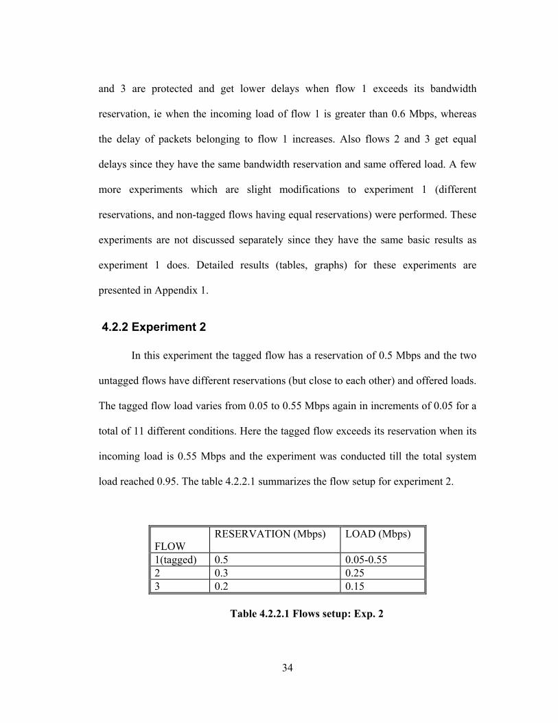
4.2.2 Experiment 2
In this experiment the tagged flow has a reservation of 0.5 Mbps and the two
untagged flows have different reservations (but close to each other) and offered loads.
The tagged flow load varies from 0.05 to 0.55 Mbps again in increments of 0.05 for a
total of 11 different conditions. Here the tagged flow exceeds its reservation when its
incoming load is 0.55 Mbps and the experiment was conducted till the total system
load reached 0.95. The table 4.2.2.1 summarizes the flow setup for experiment 2.
FLOW
RESERVATION (Mbps) LOAD (Mbps)
1(tagged) 0.5 0.05-0.55 2 0.3 0.25 3 0.2 0.15
Table 4.2.2.1 Flows setup: Exp. 2
35
Case 1:
0.05 0.1 0.15 0.2 0.25 0.3 0.35 0.4 0.45 0.5 0.550
0.02
0.04
0.06
0.08
0.1
0.12Mean Delay for various incoming loads of tagged flow
Incoming load for tagged flow (Mb/s)
Mea
n D
elay
(s)
Flow 1Flow 2Flow 3
Figure 4.2.2.1 Mean Delay for HF2Q: Exp. 2
Case 2:
0.05 0.1 0.15 0.2 0.25 0.3 0.35 0.4 0.45 0.5 0.550
0.02
0.04
0.06
0.08
0.1
0.12Mean Delay for various incoming loads of tagged flow
Incoming load for tagged flow (Mb/s)
Mea
n D
elay
(s)
Flow 1Flow 2Flow 3
Figure 4.2.2.2 Mean Delay for WFQ: Exp. 2
36
Analysis:
In this experiment we see that HF2Q exhibits the FIFO behavior irrespective
of what the reservations of the individual flows are. In this case, the tagged flow
eventually exceeds its reservation of 0.5 Mbps. We see that WFQ on the other hand
provides delays to the flows according to their individual bandwidth reservations.
Flow 1 which has a reservation of 0.5 Mbps gets the least delay so long as its
incoming load is less than its reservation. Flow 2 is seen to get a lower delay than
flow 3 since its reservation is higher and both offered loads are below their respective
reservations.
4.2.3 Experiment 3
In this experiment the three flows again have three different reservations, but
flow 1 (tagged) has a small reservation (0.2Mbps), while flow 2 has a large
reservation (0.7Mbps) and flow 3 has a very small reservation (0.1Mbps) The
experiment has two parts, both with the same weights but with different incoming
loads for the three flows. Basically this experiment differs from experiment 2 in the
fact that there is a vast difference between the reservation made by flow 2 and the
reservations of flows 1 and 3. This experiment was basically performed to test the
behavior of HF2Q even if the bandwidth reservations are largely different and to
ensure that it treats all the flows equally as FIFO does irrespective of the weights and
incoming loads.
37
4.2.3.1 Part 1
In part 1 of experiment 3 the load of the tagged flow varies from 0.05 Mbps to
0.31 Mbps; again the tagged flow exceeds its reservation. The incoming loads of
flows 2 and 3 are very close to their reservation. The experiment was repeated for 7
different tagged flow load conditions till the total system load was 0.99 Mbps. The
table 4.2.3.1.1 summarizes the flow setup for this experiment.
FLOW RESERVATION (Mbps) LOAD (Mbps) 1(tagged) 0.2 0.05-0.31 2 0.7 0.6 3 0.1 0.08
Table 4.2.3.1.1 Flows setup: Exp. 3 Case 1:
0.05 0.1 0.15 0.2 0.25 0.3 0.350
0.5
1
1.5Mean Delay for various incoming loads of tagged flow
Incoming load for tagged flow (Mb/s)
Mean D
ela
y (s
)
Flow 1Flow 2Flow 3
Figure 4.2.3.1.1 Mean Delay for HF2Q: Exp. 3
38
Case 2:
0.05 0.1 0.15 0.2 0.25 0.3 0.350
0.5
1
1.5Mean Delay for various incoming loads of tagged flow
Incoming load for tagged flow (Mb/s)
Mea
n D
elay
(s)
Flow 1Flow 2Flow 3
Figure 4.2.3.1.2 Mean Delay for WFQ: Exp. 3
Analysis:
This experiment basically demonstrates that HF2Q behaves as FIFO
irrespective of how different the reservations and the incoming loads of the different
flows are. For WFQ flow 2 gets the lowest delay throughout since it has the highest
reservation of 0.7 Mbps, even if its incoming load is much higher, but well within its
reservation. Flow 1 gets lower delays compared to flow 3 since its reservation is
higher than the other flows. But after a load of 0.2 Mbps, flow 3 gets lower delay
since flow 1 has begun to exceed its reservation and WFQ does not guarantee lower
delays for misbehaving flows.
39
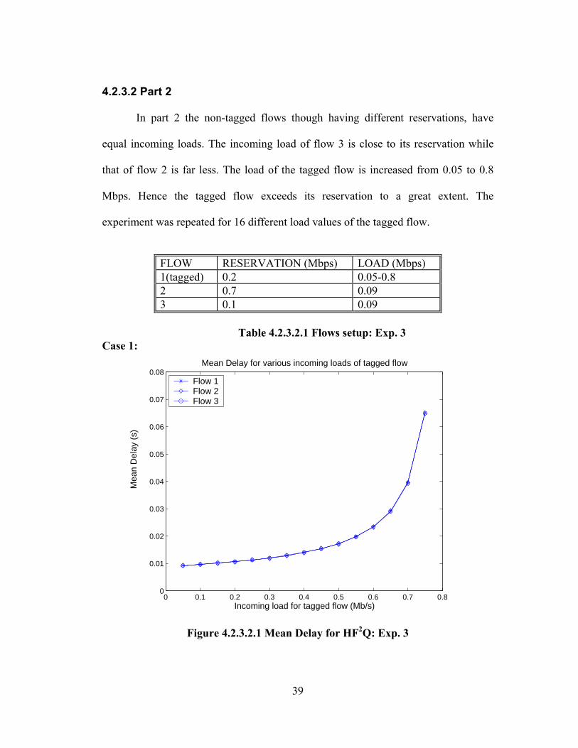
4.2.3.2 Part 2
In part 2 the non-tagged flows though having different reservations, have
equal incoming loads. The incoming load of flow 3 is close to its reservation while
that of flow 2 is far less. The load of the tagged flow is increased from 0.05 to 0.8
Mbps. Hence the tagged flow exceeds its reservation to a great extent. The
experiment was repeated for 16 different load values of the tagged flow.
FLOW RESERVATION (Mbps) LOAD (Mbps) 1(tagged) 0.2 0.05-0.8 2 0.7 0.09 3 0.1 0.09
Table 4.2.3.2.1 Flows setup: Exp. 3 Case 1:
0 0.1 0.2 0.3 0.4 0.5 0.6 0.7 0.80
0.01
0.02
0.03
0.04
0.05
0.06
0.07
0.08Mean Delay for various incoming loads of tagged flow
Incoming load for tagged flow (Mb/s)
Mea
n D
elay
(s)
Flow 1Flow 2Flow 3
Figure 4.2.3.2.1 Mean Delay for HF2Q: Exp. 3
40
Case 2:
0 0.1 0.2 0.3 0.4 0.5 0.6 0.7 0.80
0.01
0.02
0.03
0.04
0.05
0.06
0.07
0.08Mean Delay for various incoming loads of tagged flow
Incoming load for tagged flow (Mb/s)
Mea
n D
elay
(s)
Flow 1Flow 2Flow 3
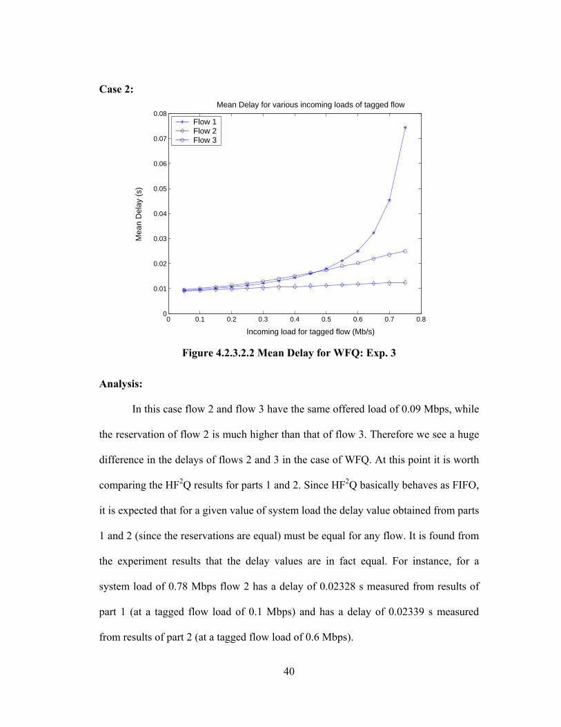
Figure 4.2.3.2.2 Mean Delay for WFQ: Exp. 3
Analysis:
In this case flow 2 and flow 3 have the same offered load of 0.09 Mbps, while
the reservation of flow 2 is much higher than that of flow 3. Therefore we see a huge
difference in the delays of flows 2 and 3 in the case of WFQ. At this point it is worth
comparing the HF2Q results for parts 1 and 2. Since HF2Q basically behaves as FIFO,
it is expected that for a given value of system load the delay value obtained from parts
1 and 2 (since the reservations are equal) must be equal for any flow. It is found from
the experiment results that the delay values are in fact equal. For instance, for a
system load of 0.78 Mbps flow 2 has a delay of 0.02328 s measured from results of
part 1 (at a tagged flow load of 0.1 Mbps) and has a delay of 0.02339 s measured
from results of part 2 (at a tagged flow load of 0.6 Mbps).
41
4.3 Mean Delay Measurements for total load > 1
The same experiments were repeated for an overloaded system, wherein the
total load offered is greater than 1. Again a comparison was made between the
performance of HF2Q and WFQ. With the current Internet and broadband revolution,
the network must handle increasingly large volumes of data, which can lead to
network overload and signal degradation. Hence queuing algorithms that control the
order in which packets are sent, and the usage of the gateway buffer space, and the
way in which packets from different sources interact play an important part in
congestion control. Hence it is important that the performance of this new queuing
algorithm under overloaded conditions is characterized and a comparison made to the
existing WFQ. In all of these experiments two sets of results for the HF2Q and WFQ
are shown – one set (shown in case 1) that includes the all the delay values of the
flows including the values for a total system load of 1, and another set (shown in case
2) that does not show the values of load for which the system exhibits a transitional
behavior of HF2Q. In all the results shown below, the delay of the tagged flow, which
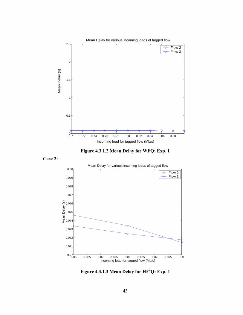
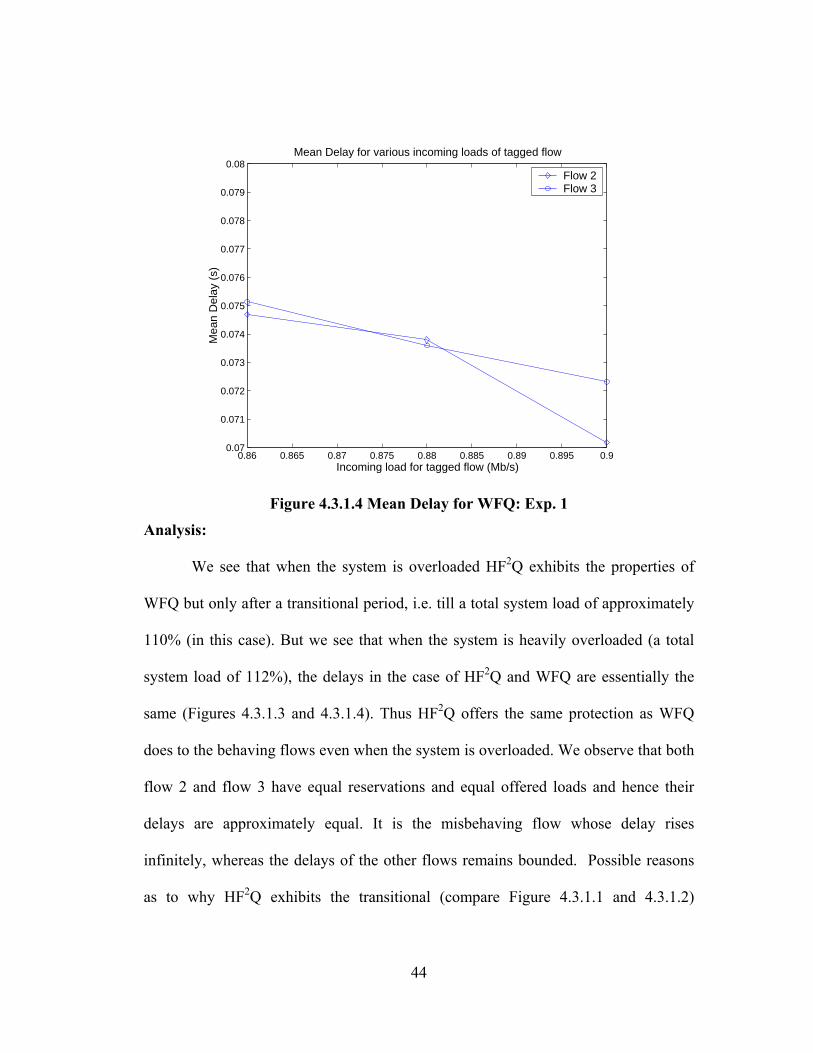
rises infinitely, is not plotted. In the following description, the experiments
correspond to those described in section 4.2 (underloaded case).
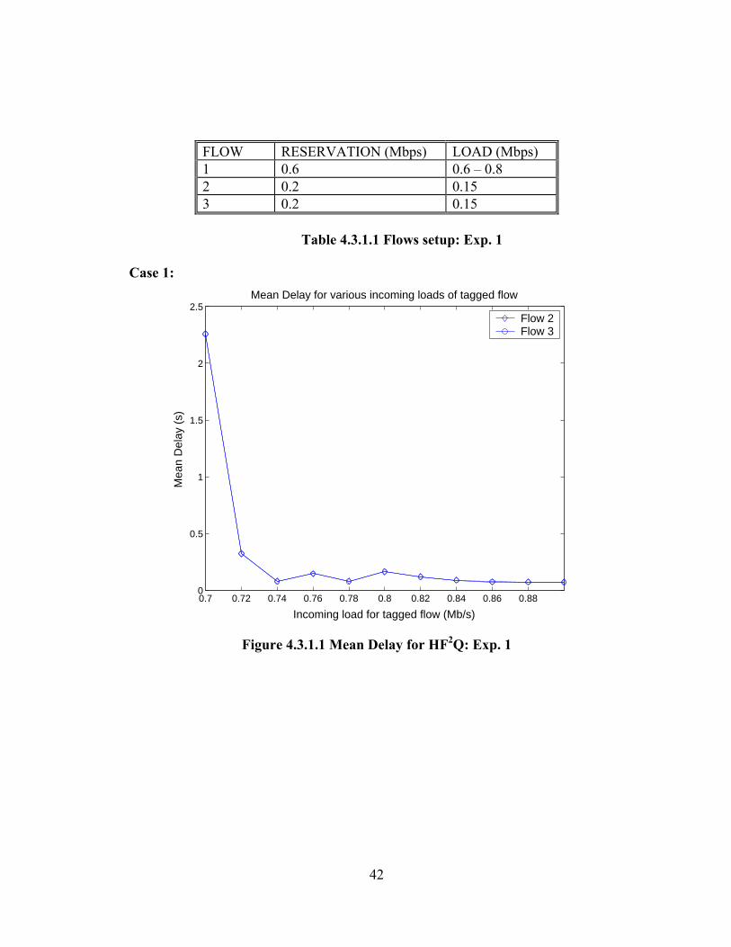
4.3.1 Experiment 1
The load of the tagged flow is increased from 0.6 Mbps (100% system load)
to 0.8 Mbps (120% system load), while the load of the other two flows are maintained
below their reservations. The experiment was repeated for 11 different loads of the
tagged flow. Table 4.3.1.1 summarizes the flow setup.
42
FLOW RESERVATION (Mbps) LOAD (Mbps) 1 0.6 0.6 – 0.8 2 0.2 0.15 3 0.2 0.15
Table 4.3.1.1 Flows setup: Exp. 1 Case 1:
0.7 0.72 0.74 0.76 0.78 0.8 0.82 0.84 0.86 0.880
0.5
1
1.5
2
2.5Mean Delay for various incoming loads of tagged flow
Incoming load for tagged flow (Mb/s)
Mea
n D
elay
(s)
Flow 2Flow 3
Figure 4.3.1.1 Mean Delay for HF2Q: Exp. 1
43
0.7 0.72 0.74 0.76 0.78 0.8 0.82 0.84 0.86 0.880
0.5
1
1.5
2
2.5Mean Delay for various incoming loads of tagged flow
Incoming load for tagged flow (Mb/s)
Mea
n D
elay
(s)
Flow 2Flow 3
Figure 4.3.1.2 Mean Delay for WFQ: Exp. 1
Case 2:
0.86 0.865 0.87 0.875 0.88 0.885 0.89 0.895 0.90.07
0.071
0.072
0.073
0.074
0.075
0.076
0.077
0.078
0.079
0.08Mean Delay for various incoming loads of tagged flow
Incoming load for tagged flow (Mb/s)
Mea
n D
elay
(s)
Flow 2Flow 3
Figure 4.3.1.3 Mean Delay for HF2Q: Exp. 1
44
0.86 0.865 0.87 0.875 0.88 0.885 0.89 0.895 0.90.07
0.071
0.072
0.073
0.074
0.075
0.076
0.077
0.078
0.079
0.08Mean Delay for various incoming loads of tagged flow
Incoming load for tagged flow (Mb/s)
Mea
n D
elay
(s)
Flow 2Flow 3
Figure 4.3.1.4 Mean Delay for WFQ: Exp. 1
Analysis:
We see that when the system is overloaded HF2Q exhibits the properties of
WFQ but only after a transitional period, i.e. till a total system load of approximately
110% (in this case). But we see that when the system is heavily overloaded (a total
system load of 112%), the delays in the case of HF2Q and WFQ are essentially the
same (Figures 4.3.1.3 and 4.3.1.4). Thus HF2Q offers the same protection as WFQ
does to the behaving flows even when the system is overloaded. We observe that both
flow 2 and flow 3 have equal reservations and equal offered loads and hence their
delays are approximately equal. It is the misbehaving flow whose delay rises
infinitely, whereas the delays of the other flows remains bounded. Possible reasons
as to why HF2Q exhibits the transitional (compare Figure 4.3.1.1 and 4.3.1.2)
45
behavior are presented in the section 4.5. As for the underloaded case the detailed
results for similar experiments are presented in Appendix 1.
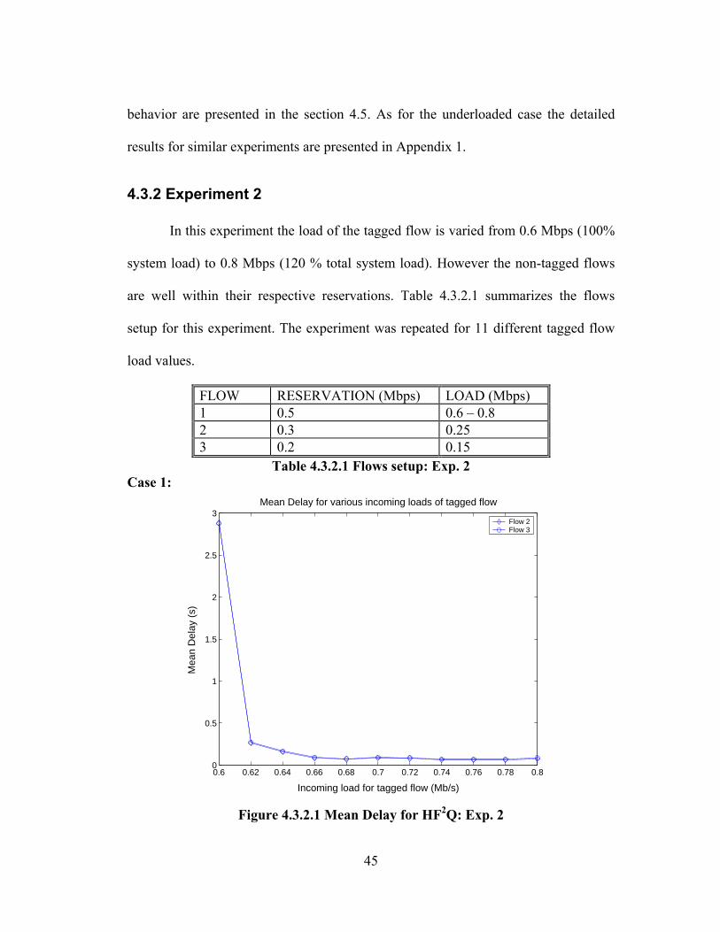
4.3.2 Experiment 2
In this experiment the load of the tagged flow is varied from 0.6 Mbps (100%
system load) to 0.8 Mbps (120 % total system load). However the non-tagged flows
are well within their respective reservations. Table 4.3.2.1 summarizes the flows
setup for this experiment. The experiment was repeated for 11 different tagged flow
load values.
FLOW RESERVATION (Mbps) LOAD (Mbps) 1 0.5 0.6 – 0.8 2 0.3 0.25 3 0.2 0.15
Table 4.3.2.1 Flows setup: Exp. 2 Case 1:
0.6 0.62 0.64 0.66 0.68 0.7 0.72 0.74 0.76 0.78 0.80
0.5
1
1.5
2
2.5
3Mean Delay for various incoming loads of tagged flow
Incoming load for tagged flow (Mb/s)
Mea
n D
elay
(s)
Flow 2Flow 3
Figure 4.3.2.1 Mean Delay for HF2Q: Exp. 2
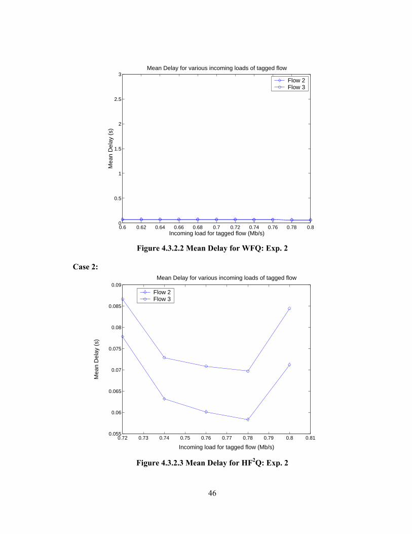
46
0.6 0.62 0.64 0.66 0.68 0.7 0.72 0.74 0.76 0.78 0.80
0.5
1
1.5
2
2.5
3Mean Delay for various incoming loads of tagged flow
Incoming load for tagged flow (Mb/s)
Mea
n D
elay
(s)
Flow 2Flow 3
Figure 4.3.2.2 Mean Delay for WFQ: Exp. 2
Case 2:
0.72 0.73 0.74 0.75 0.76 0.77 0.78 0.79 0.8 0.810.055
0.06
0.065
0.07
0.075
0.08
0.085
0.09Mean Delay for various incoming loads of tagged flow
Incoming load for tagged flow (Mb/s)
Mea
n D
elay
(s)
Flow 2Flow 3
Figure 4.3.2.3 Mean Delay for HF2Q: Exp. 2
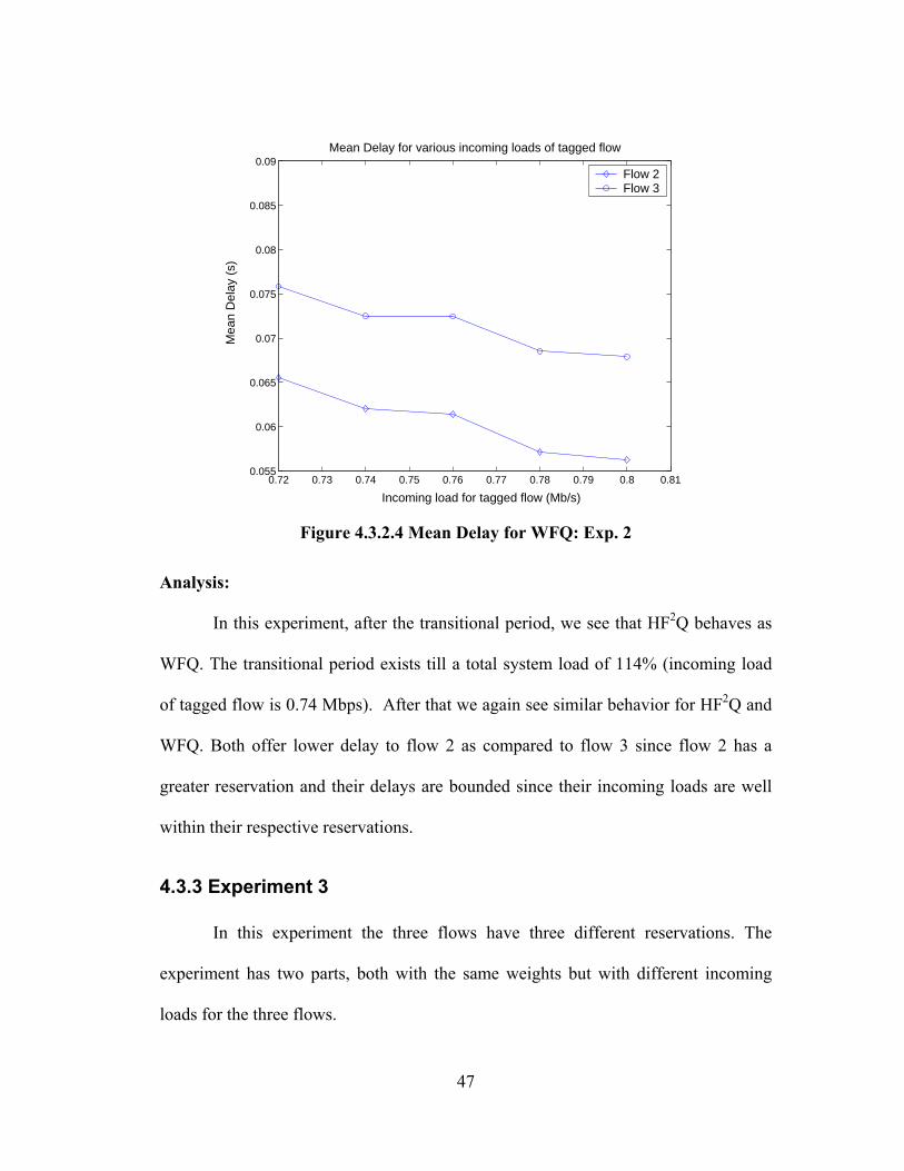
47
0.72 0.73 0.74 0.75 0.76 0.77 0.78 0.79 0.8 0.810.055
0.06
0.065
0.07
0.075
0.08
0.085
0.09Mean Delay for various incoming loads of tagged flow
Incoming load for tagged flow (Mb/s)
Mea
n D
elay
(s)
Flow 2Flow 3
Figure 4.3.2.4 Mean Delay for WFQ: Exp. 2
Analysis:
In this experiment, after the transitional period, we see that HF2Q behaves as
WFQ. The transitional period exists till a total system load of 114% (incoming load
of tagged flow is 0.74 Mbps). After that we again see similar behavior for HF2Q and
WFQ. Both offer lower delay to flow 2 as compared to flow 3 since flow 2 has a
greater reservation and their delays are bounded since their incoming loads are well
within their respective reservations.
4.3.3 Experiment 3 In this experiment the three flows have three different reservations. The
experiment has two parts, both with the same weights but with different incoming
loads for the three flows.
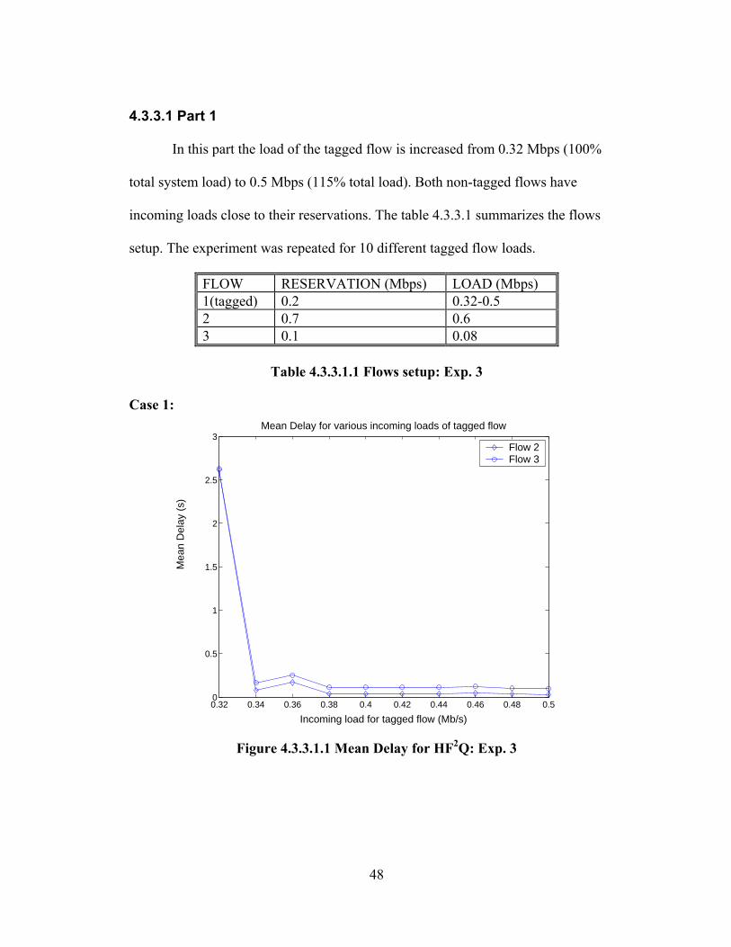
48
4.3.3.1 Part 1
In this part the load of the tagged flow is increased from 0.32 Mbps (100%
total system load) to 0.5 Mbps (115% total load). Both non-tagged flows have
incoming loads close to their reservations. The table 4.3.3.1 summarizes the flows
setup. The experiment was repeated for 10 different tagged flow loads.
FLOW RESERVATION (Mbps) LOAD (Mbps) 1(tagged) 0.2 0.32-0.5 2 0.7 0.6 3 0.1 0.08
Table 4.3.3.1.1 Flows setup: Exp. 3
Case 1:
0.32 0.34 0.36 0.38 0.4 0.42 0.44 0.46 0.48 0.50
0.5
1
1.5
2
2.5
3Mean Delay for various incoming loads of tagged flow
Incoming load for tagged flow (Mb/s)
Mea
n D
elay
(s)
Flow 2Flow 3
Figure 4.3.3.1.1 Mean Delay for HF2Q: Exp. 3
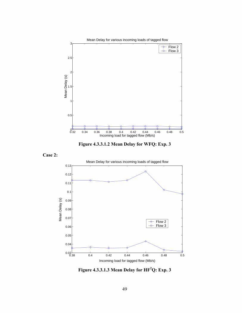
49
0.32 0.34 0.36 0.38 0.4 0.42 0.44 0.46 0.48 0.50
0.5
1
1.5
2
2.5
3Mean Delay for various incoming loads of tagged flow
Incoming load for tagged flow (Mb/s)
Mea
n D
elay
(s)
Flow 2Flow 3
Figure 4.3.3.1.2 Mean Delay for WFQ: Exp. 3
Case 2:
0.38 0.4 0.42 0.44 0.46 0.48 0.50.03
0.04
0.05
0.06
0.07
0.08
0.09
0.1
0.11
0.12
0.13Mean Delay for various incoming loads of tagged flow
Incoming load for tagged flow (Mb/s)
Mea
n D
elay
(s)
Flow 2Flow 3
Figure 4.3.3.1.3 Mean Delay for HF2Q: Exp. 3
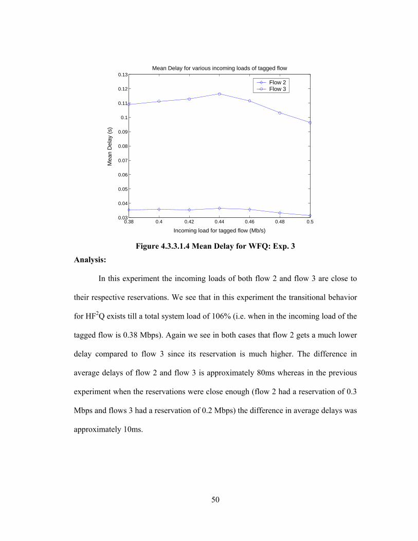
50
0.38 0.4 0.42 0.44 0.46 0.48 0.50.03
0.04
0.05
0.06
0.07
0.08
0.09
0.1
0.11
0.12
0.13Mean Delay for various incoming loads of tagged flow
Incoming load for tagged flow (Mb/s)
Mea
n D
elay
(s)
Flow 2Flow 3
Figure 4.3.3.1.4 Mean Delay for WFQ: Exp. 3
Analysis:
In this experiment the incoming loads of both flow 2 and flow 3 are close to
their respective reservations. We see that in this experiment the transitional behavior
for HF2Q exists till a total system load of 106% (i.e. when in the incoming load of the
tagged flow is 0.38 Mbps). Again we see in both cases that flow 2 gets a much lower
delay compared to flow 3 since its reservation is much higher. The difference in
average delays of flow 2 and flow 3 is approximately 80ms whereas in the previous
experiment when the reservations were close enough (flow 2 had a reservation of 0.3
Mbps and flows 3 had a reservation of 0.2 Mbps) the difference in average delays was
approximately 10ms.
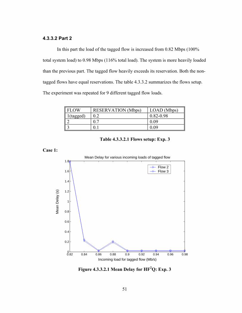
51
4.3.3.2 Part 2
In this part the load of the tagged flow is increased from 0.82 Mbps (100%
total system load) to 0.98 Mbps (116% total load). The system is more heavily loaded
than the previous part. The tagged flow heavily exceeds its reservation. Both the non-
tagged flows have equal reservations. The table 4.3.3.2 summarizes the flows setup.
The experiment was repeated for 9 different tagged flow loads.
FLOW RESERVATION (Mbps) LOAD (Mbps) 1(tagged) 0.2 0.82-0.98 2 0.7 0.09 3 0.1 0.09
Table 4.3.3.2.1 Flows setup: Exp. 3 Case 1:
0.82 0.84 0.86 0.88 0.9 0.92 0.94 0.96 0.980
0.2
0.4
0.6
0.8
1
1.2
1.4
1.6
1.8Mean Delay for various incoming loads of tagged flow
Incoming load for tagged flow (Mb/s)
Mea
n D
elay
(s)
Flow 2Flow 3
Figure 4.3.3.2.1 Mean Delay for HF2Q: Exp. 3
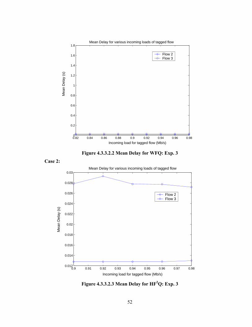
52
0.82 0.84 0.86 0.88 0.9 0.92 0.94 0.96 0.980
0.2
0.4
0.6
0.8
1
1.2
1.4
1.6
1.8Mean Delay for various incoming loads of tagged flow
Incoming load for tagged flow (Mb/s)
Mea
n D
elay
(s)
Flow 2Flow 3
Figure 4.3.3.2.2 Mean Delay for WFQ: Exp. 3
Case 2:
0.9 0.91 0.92 0.93 0.94 0.95 0.96 0.97 0.980.012
0.014
0.016
0.018
0.02
0.022
0.024
0.026
0.028
0.03Mean Delay for various incoming loads of tagged flow
Incoming load for tagged flow (Mb/s)
Mea
n D
elay
(s)
Flow 2Flow 3
Figure 4.3.3.2.3 Mean Delay for HF2Q: Exp. 3
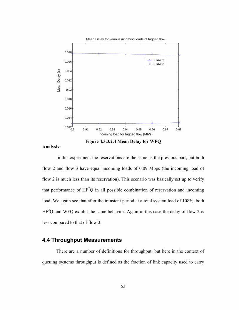
53
0.9 0.91 0.92 0.93 0.94 0.95 0.96 0.97 0.980.012
0.014
0.016
0.018
0.02
0.022
0.024
0.026
0.028
Mean Delay for various incoming loads of tagged flow
Incoming load for tagged flow (Mb/s)
Mea
n D
elay
(s)
Flow 2Flow 3
Figure 4.3.3.2.4 Mean Delay for WFQ
Analysis:
In this experiment the reservations are the same as the previous part, but both
flow 2 and flow 3 have equal incoming loads of 0.09 Mbps (the incoming load of
flow 2 is much less than its reservation). This scenario was basically set up to verify
that performance of HF2Q in all possible combination of reservation and incoming
load. We again see that after the transient period at a total system load of 108%, both
HF2Q and WFQ exhibit the same behavior. Again in this case the delay of flow 2 is
less compared to that of flow 3.
4.4 Throughput Measurements
There are a number of definitions for throughput, but here in the context of
queuing systems throughput is defined as the fraction of link capacity used to carry
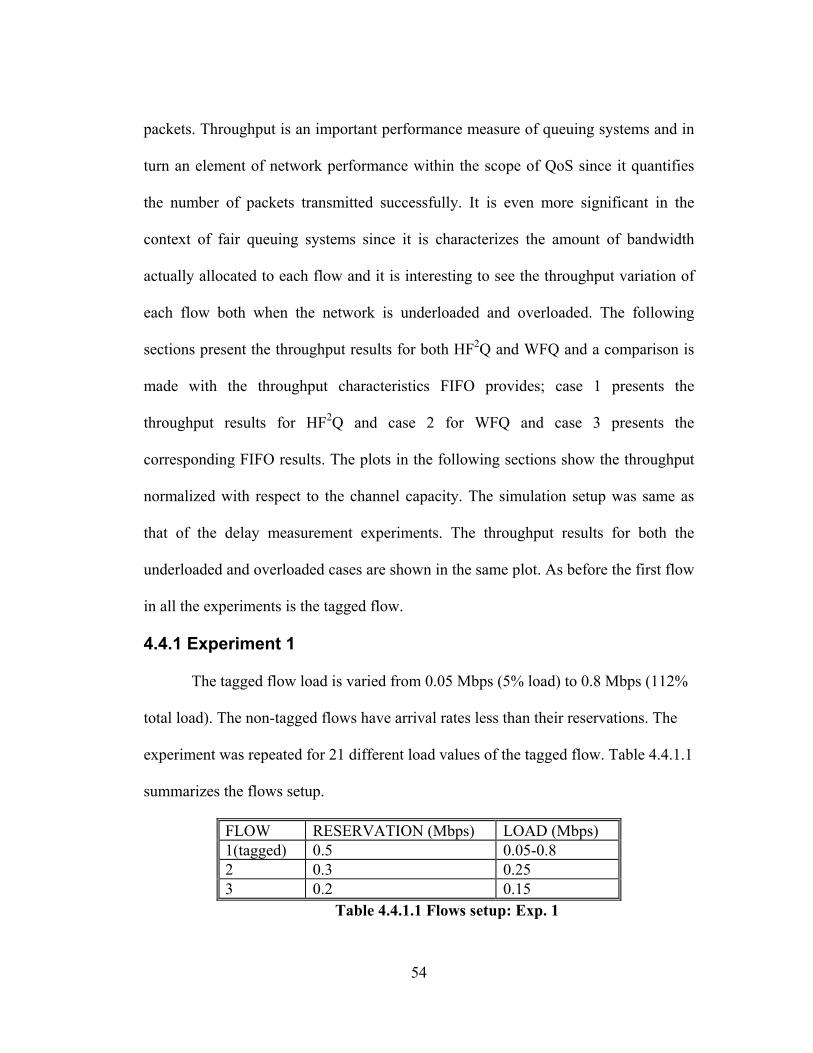
54
packets. Throughput is an important performance measure of queuing systems and in
turn an element of network performance within the scope of QoS since it quantifies
the number of packets transmitted successfully. It is even more significant in the
context of fair queuing systems since it is characterizes the amount of bandwidth
actually allocated to each flow and it is interesting to see the throughput variation of
each flow both when the network is underloaded and overloaded. The following
sections present the throughput results for both HF2Q and WFQ and a comparison is
made with the throughput characteristics FIFO provides; case 1 presents the
throughput results for HF2Q and case 2 for WFQ and case 3 presents the
corresponding FIFO results. The plots in the following sections show the throughput
normalized with respect to the channel capacity. The simulation setup was same as
that of the delay measurement experiments. The throughput results for both the
underloaded and overloaded cases are shown in the same plot. As before the first flow
in all the experiments is the tagged flow.
4.4.1 Experiment 1
The tagged flow load is varied from 0.05 Mbps (5% load) to 0.8 Mbps (112%
total load). The non-tagged flows have arrival rates less than their reservations. The
experiment was repeated for 21 different load values of the tagged flow. Table 4.4.1.1
summarizes the flows setup.
FLOW RESERVATION (Mbps) LOAD (Mbps) 1(tagged) 0.5 0.05-0.8 2 0.3 0.25 3 0.2 0.15
Table 4.4.1.1 Flows setup: Exp. 1
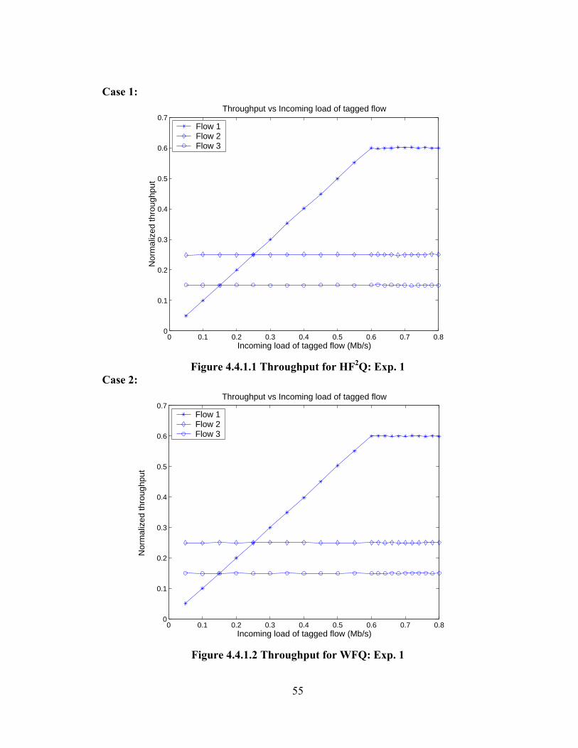
55
Case 1:
0 0.1 0.2 0.3 0.4 0.5 0.6 0.7 0.80
0.1
0.2
0.3
0.4
0.5
0.6
0.7Throughput vs Incoming load of tagged flow
Incoming load of tagged flow (Mb/s)
Nor
mal
ized
thro
ughp
ut
Flow 1Flow 2Flow 3
Figure 4.4.1.1 Throughput for HF2Q: Exp. 1
Case 2:
0 0.1 0.2 0.3 0.4 0.5 0.6 0.7 0.80
0.1
0.2
0.3
0.4
0.5
0.6
0.7Throughput vs Incoming load of tagged flow
Incoming load of tagged flow (Mb/s)
Nor
mal
ized
thro
ughp
ut
Flow 1Flow 2Flow 3
Figure 4.4.1.2 Throughput for WFQ: Exp. 1
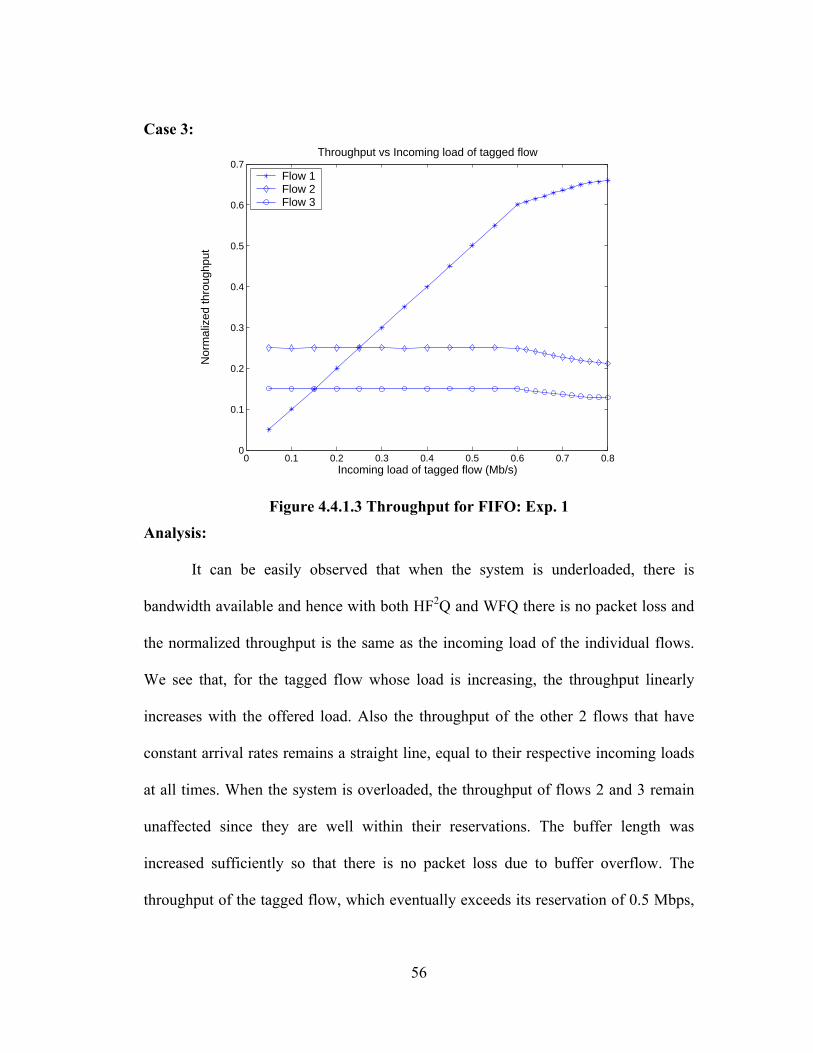
56
Case 3:
0 0.1 0.2 0.3 0.4 0.5 0.6 0.7 0.80
0.1
0.2
0.3
0.4
0.5
0.6
0.7Throughput vs Incoming load of tagged flow
Incoming load of tagged flow (Mb/s)
Nor
mal
ized
thro
ughp
ut
Flow 1Flow 2Flow 3
Figure 4.4.1.3 Throughput for FIFO: Exp. 1
Analysis: It can be easily observed that when the system is underloaded, there is
bandwidth available and hence with both HF2Q and WFQ there is no packet loss and
the normalized throughput is the same as the incoming load of the individual flows.
We see that, for the tagged flow whose load is increasing, the throughput linearly
increases with the offered load. Also the throughput of the other 2 flows that have
constant arrival rates remains a straight line, equal to their respective incoming loads
at all times. When the system is overloaded, the throughput of flows 2 and 3 remain
unaffected since they are well within their reservations. The buffer length was
increased sufficiently so that there is no packet loss due to buffer overflow. The
throughput of the tagged flow, which eventually exceeds its reservation of 0.5 Mbps,
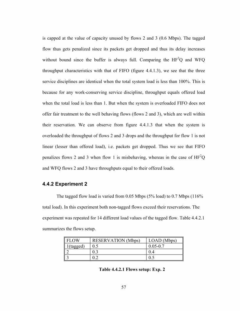
57
is capped at the value of capacity unused by flows 2 and 3 (0.6 Mbps). The tagged
flow thus gets penalized since its packets get dropped and thus its delay increases
without bound since the buffer is always full. Comparing the HF2Q and WFQ
throughput characteristics with that of FIFO (figure 4.4.1.3), we see that the three
service disciplines are identical when the total system load is less than 100%. This is
because for any work-conserving service discipline, throughput equals offered load
when the total load is less than 1. But when the system is overloaded FIFO does not
offer fair treatment to the well behaving flows (flows 2 and 3), which are well within
their reservation. We can observe from figure 4.4.1.3 that when the system is
overloaded the throughput of flows 2 and 3 drops and the throughput for flow 1 is not
linear (lesser than offered load), i.e. packets get dropped. Thus we see that FIFO
penalizes flows 2 and 3 when flow 1 is misbehaving, whereas in the case of HF2Q
and WFQ flows 2 and 3 have throughputs equal to their offered loads.
4.4.2 Experiment 2
The tagged flow load is varied from 0.05 Mbps (5% load) to 0.7 Mbps (116%
total load). In this experiment both non-tagged flows exceed their reservations. The
experiment was repeated for 14 different load values of the tagged flow. Table 4.4.2.1
summarizes the flows setup.
FLOW RESERVATION (Mbps) LOAD (Mbps) 1(tagged) 0.5 0.05-0.7 2 0.3 0.4 3 0.2 0.5
Table 4.4.2.1 Flows setup: Exp. 2
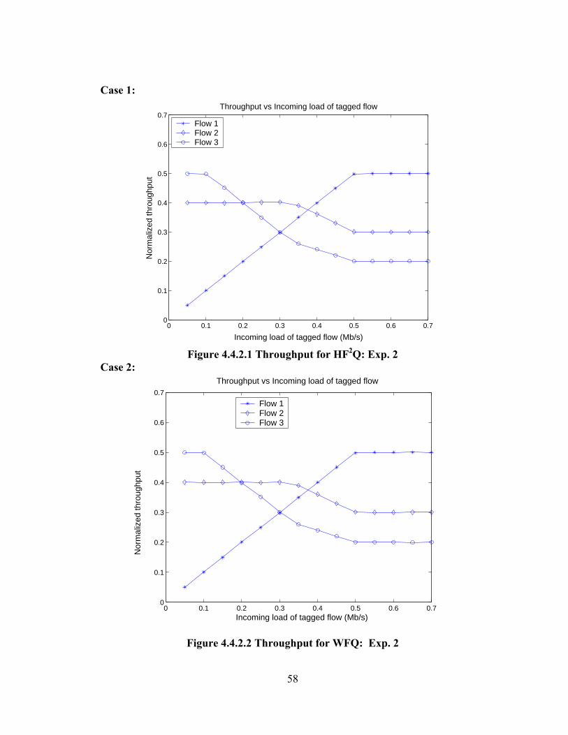
58
Case 1:
0 0.1 0.2 0.3 0.4 0.5 0.6 0.70
0.1
0.2
0.3
0.4
0.5
0.6
0.7Throughput vs Incoming load of tagged flow
Incoming load of tagged flow (Mb/s)
Nor
mal
ized
thro
ughp
ut
Flow 1Flow 2Flow 3
Figure 4.4.2.1 Throughput for HF2Q: Exp. 2
Case 2:
0 0.1 0.2 0.3 0.4 0.5 0.6 0.70
0.1
0.2
0.3
0.4
0.5
0.6
0.7
Throughput vs Incoming load of tagged flow
Incoming load of tagged flow (Mb/s)
Nor
mal
ized
thro
ughp
ut
Flow 1Flow 2Flow 3
Figure 4.4.2.2 Throughput for WFQ: Exp. 2
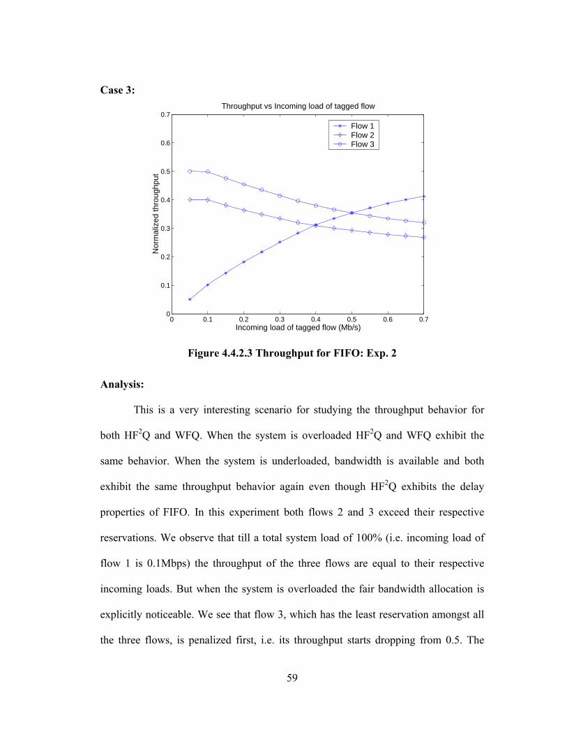
59
Case 3:
0 0.1 0.2 0.3 0.4 0.5 0.6 0.70
0.1
0.2
0.3
0.4
0.5
0.6
0.7Throughput vs Incoming load of tagged flow
Incoming load of tagged flow (Mb/s)
Nor
mal
ized
thro
ughp
ut
Flow 1Flow 2Flow 3
Figure 4.4.2.3 Throughput for FIFO: Exp. 2
Analysis:
This is a very interesting scenario for studying the throughput behavior for
both HF2Q and WFQ. When the system is overloaded HF2Q and WFQ exhibit the
same behavior. When the system is underloaded, bandwidth is available and both
exhibit the same throughput behavior again even though HF2Q exhibits the delay
properties of FIFO. In this experiment both flows 2 and 3 exceed their respective
reservations. We observe that till a total system load of 100% (i.e. incoming load of
flow 1 is 0.1Mbps) the throughput of the three flows are equal to their respective
incoming loads. But when the system is overloaded the fair bandwidth allocation is
explicitly noticeable. We see that flow 3, which has the least reservation amongst all
the three flows, is penalized first, i.e. its throughput starts dropping from 0.5. The
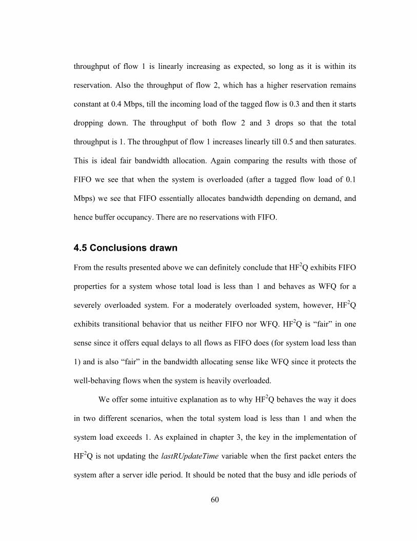
60
throughput of flow 1 is linearly increasing as expected, so long as it is within its
reservation. Also the throughput of flow 2, which has a higher reservation remains
constant at 0.4 Mbps, till the incoming load of the tagged flow is 0.3 and then it starts
dropping down. The throughput of both flow 2 and 3 drops so that the total
throughput is 1. The throughput of flow 1 increases linearly till 0.5 and then saturates.
This is ideal fair bandwidth allocation. Again comparing the results with those of
FIFO we see that when the system is overloaded (after a tagged flow load of 0.1
Mbps) we see that FIFO essentially allocates bandwidth depending on demand, and
hence buffer occupancy. There are no reservations with FIFO.
4.5 Conclusions drawn From the results presented above we can definitely conclude that HF2Q exhibits FIFO
properties for a system whose total load is less than 1 and behaves as WFQ for a
severely overloaded system. For a moderately overloaded system, however, HF2Q
exhibits transitional behavior that us neither FIFO nor WFQ. HF2Q is “fair” in one
sense since it offers equal delays to all flows as FIFO does (for system load less than
1) and is also “fair” in the bandwidth allocating sense like WFQ since it protects the
well-behaving flows when the system is heavily overloaded.
We offer some intuitive explanation as to why HF2Q behaves the way it does
in two different scenarios, when the total system load is less than 1 and when the
system load exceeds 1. As explained in chapter 3, the key in the implementation of
HF2Q is not updating the lastRUpdateTime variable when the first packet enters the
system after a server idle period. It should be noted that the busy and idle periods of
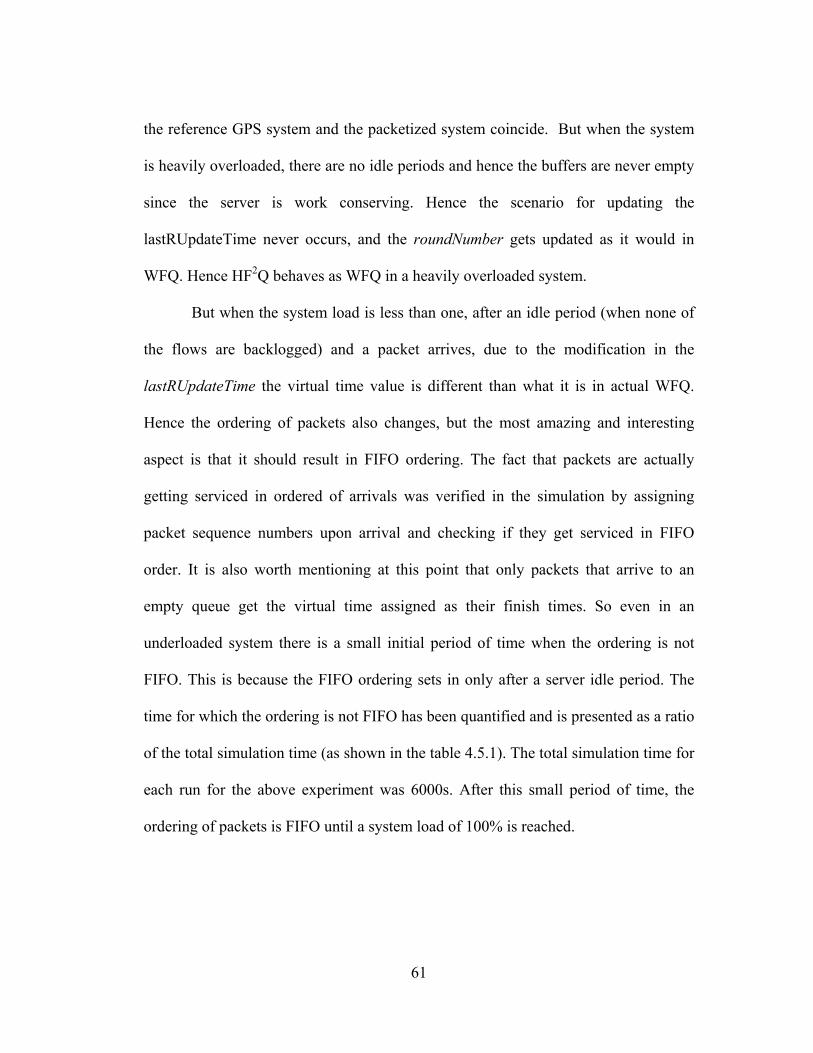
61
the reference GPS system and the packetized system coincide. But when the system
is heavily overloaded, there are no idle periods and hence the buffers are never empty
since the server is work conserving. Hence the scenario for updating the
lastRUpdateTime never occurs, and the roundNumber gets updated as it would in
WFQ. Hence HF2Q behaves as WFQ in a heavily overloaded system.
But when the system load is less than one, after an idle period (when none of
the flows are backlogged) and a packet arrives, due to the modification in the
lastRUpdateTime the virtual time value is different than what it is in actual WFQ.
Hence the ordering of packets also changes, but the most amazing and interesting
aspect is that it should result in FIFO ordering. The fact that packets are actually
getting serviced in ordered of arrivals was verified in the simulation by assigning
packet sequence numbers upon arrival and checking if they get serviced in FIFO
order. It is also worth mentioning at this point that only packets that arrive to an
empty queue get the virtual time assigned as their finish times. So even in an
underloaded system there is a small initial period of time when the ordering is not
FIFO. This is because the FIFO ordering sets in only after a server idle period. The
time for which the ordering is not FIFO has been quantified and is presented as a ratio
of the total simulation time (as shown in the table 4.5.1). The total simulation time for
each run for the above experiment was 6000s. After this small period of time, the
ordering of packets is FIFO until a system load of 100% is reached.
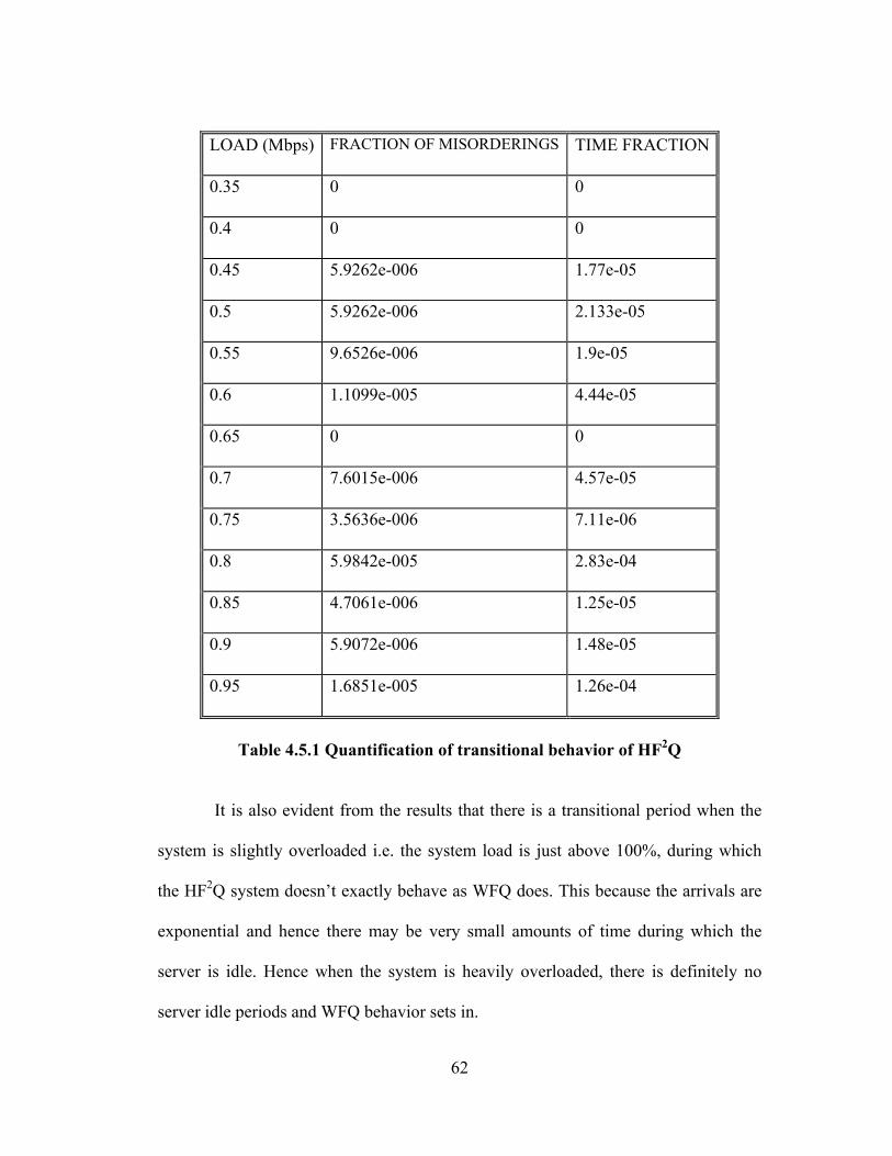
62
LOAD (Mbps) FRACTION OF MISORDERINGS TIME FRACTION
0.35 0 0
0.4 0 0
0.45 5.9262e-006 1.77e-05
0.5 5.9262e-006 2.133e-05
0.55 9.6526e-006 1.9e-05
0.6 1.1099e-005 4.44e-05
0.65 0 0
0.7 7.6015e-006 4.57e-05
0.75 3.5636e-006 7.11e-06
0.8 5.9842e-005 2.83e-04
0.85 4.7061e-006 1.25e-05
0.9 5.9072e-006 1.48e-05
0.95 1.6851e-005 1.26e-04
Table 4.5.1 Quantification of transitional behavior of HF2Q
It is also evident from the results that there is a transitional period when the
system is slightly overloaded i.e. the system load is just above 100%, during which
the HF2Q system doesn’t exactly behave as WFQ does. This because the arrivals are
exponential and hence there may be very small amounts of time during which the
server is idle. Hence when the system is heavily overloaded, there is definitely no
server idle periods and WFQ behavior sets in.
63
5 DOCSIS Performance Evaluation
As mentioned in Chapter 1, the objective of this thesis was two-fold, one to
characterize the performance of a new queuing discipline and the other to evaluate the
performance of DOCSIS 1.1. Chapters 3 and 4 presented a detailed evaluation of
HF2Q. This chapter presents a detailed performance evaluation of DOCSIS 1.1 in the
context of BWA networks.
Hybrid Fiber Coax (HFC) cable networks have been used in the past primarily
to deliver broadcast-quality TV signals to homes. The wide availability of such
systems and their extremely wide bandwidth allows extending their functionality to
deliver high-speed broadband data signals to end-users. Data over Cable System
Interface Specifications (DOCSIS), a MAC protocol elaborated under the leadership
of Cable Television Laboratories, Inc., has been established as the major industry
standard for two-way communications over HFC cable plants. The first
specifications, referred to as DOCSIS 1.0, have been largely deployed in cable
networks. The second specifications (DOCSIS 1.1) are now in the early phase of
deployment. The physical layer of DOCSIS 1.1 specifications is the same as that of
DOCSIS 1.0. The difference between the two sets of specifications lies on the MAC
layer, which includes Quality of Service (QoS) capabilities, in DOCSIS 1.1
specifications. This has been adopted as the de facto standard for delivering
broadband services for HFC networks. Although DOCSIS is designed for
interoperability among cable modems and related products, with a few modifications
it can be used in wireless Multipoint, Multichannel Distribution Service (MMDS) and
64
Local Multipoint Distribution Service (LMDS) systems. Such Broadband Wireless
Access (BWA) networks attempt to carry high speed Internet traffic to subscriber
systems, are easy to implement and can be installed without extensive infrastructure.
Hence, The IEEE802.16 standard developed for BWA systems was based on two
HFC MAC protocols, IEEE 802.14a and DOCSIS. This is due to the striking
similarities between the cable medium and the wireless environment.
5.1 DOCSIS 1.1 Overview
5.1.1 DOCSIS 1.1 Basics
DOCSIS 1.1 is an IP-centric point-to-multipoint standard that was developed
for broadband Internet access applications over cable TV networks. DOCIS specifies
both the physical layer and the Medium Access Control (MAC) layer. Its major
components are the Cable Modems (CM) at the customer premises and the Cable
Modem Termination System (CMTS) at the head-end of the cable plant. DOCSIS 1.1
evolved from the DOCSIS 1.0 specs, but with Quality of Service (QoS) mechanisms
and algorithms implemented at the MAC layer. To summarize, DOCSIS 1.1 builds
upon 1.0, but also includes the following features:
• Quality of Service
• Dynamic Services
• Concatenation
• Fragmentation
• Payload Header Suppression
65
• IP Multicast
• CM Authentication
• SNMPv3
• CM Account Management
• Fault Management
• Secure Software
The medium between the CMTS and the different CMs is a two-way shared
medium, in which the downstream channels carry signals from the head-end to users
and upstream channels carry signals from users to head-end. Upstream and
downstream channels are separated using Frequency Division Duplex (FDD). A CM
is normally tuned to one upstream channel and the associated downstream channel.
The upstream channel is an inherently shared medium while the downstream is a
broadcast dedicated link from the CMTS to the CMs.
DOCSIS has a reservation-based, centralized approach for allocating
bandwidth and scheduling packet transmissions on the upstream channel. The
upstream is modeled as a stream of mini-lots, with a dynamic mix of contention and
reservation-based transmission opportunities. CMs may use the contention mini-slots
for transmitting their requests, and the CMTS allocates (schedules) transmission
opportunities for the CMs in the next frame if capacity is available. Periodically, the
CMTS sends a Bandwidth Allocation Map (MAP) message over the downstream
channel to indicate to the CMs the specific mini-lots allocated to them. The
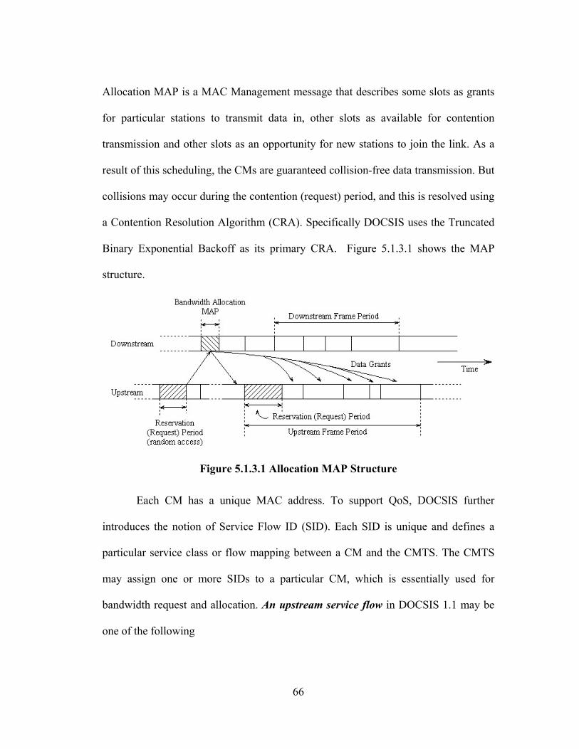
66
Allocation MAP is a MAC Management message that describes some slots as grants
for particular stations to transmit data in, other slots as available for contention
transmission and other slots as an opportunity for new stations to join the link. As a
result of this scheduling, the CMs are guaranteed collision-free data transmission. But
collisions may occur during the contention (request) period, and this is resolved using
a Contention Resolution Algorithm (CRA). Specifically DOCSIS uses the Truncated
Binary Exponential Backoff as its primary CRA. Figure 5.1.3.1 shows the MAP
structure.
Figure 5.1.3.1 Allocation MAP Structure
Each CM has a unique MAC address. To support QoS, DOCSIS further
introduces the notion of Service Flow ID (SID). Each SID is unique and defines a
particular service class or flow mapping between a CM and the CMTS. The CMTS
may assign one or more SIDs to a particular CM, which is essentially used for
bandwidth request and allocation. An upstream service flow in DOCSIS 1.1 may be
one of the following
67
• Unsolicited Grant Service (UGS)
• Real-time Polling Service (rtPS)
• Non-Real-time Polling Service (nrtPS)
• Best Effort (BE)
• Unsolicited Grant Service with Activity Detection (UGS-AD)
Other key enhancements made in DOCSIS 1.1 are
• Support for multiple service flows per cable modem allows a single modem to
support a combination of video, voice and data packets.
• Dynamic service establishment allows MAC messages to dynamically create,
modify and delete traffic flows.
• Layer 2 fragmentation allows fragmenting larger data packets
• Concatenation allows CMs to send multiple MAC frames in the same
transmission
5.1.2 Upstream Bandwidth Allocation:
There are a number of ways by which the CM can obtain bandwidth for data
transmission from the CMTS:
a) By making explicit requests through contention, piggybacking or unicast
opportunities
b) Unsolicited grants
68
Contention:
Portions of the upstream bandwidth are open to all modems (contention) for
requesting upstream bandwidth. The requests transmitted through contention are
subject to collision, and these collisions are resolved by a Contention Resolution
Algorithm.
Piggybacking:
Piggyback is a request for additional bandwidth sent in a data transmission.
Piggybacking obviates contention, since the requests are transmitted with the data
packets.
Unicast Request Polls:
Periodic unicast request opportunities are sent as a means of real-time polls regardless
of network congestion. These opportunities in the Allocation MAP (see below) may
be used by the stations to transmit their request packets, avoiding contention. The
allocation MAP is a varying length MAC Management message that is transmitted by
the CMTS to define the transmission opportunities on the upstream. It includes a
fixed-length header followed by variable number of Information Elements (IEs). Each
IE defines the allowed usage for a range of minislots. Each IE consists of a 14-bit
SID, a 4-bit type code and a 14-bit starting offset. The four defined types of SIDs are
broadcast (intended for all stations), multicast (intended for a group of stations),
unicast (intended for a particular station) and a null address (intended for no station).
The various IEs that the CMTS may send in the MAP are:
69
• Request IE – provides intervals in which requests may be made for
bandwidths for upstream data transmission
• Request/Data IE – provides intervals in which requests for bandwidth or short
data packets may be transmitted
• Initial Maintenance IE – provides intervals in which new stations may join the
network
• Station Maintenance IE - provides intervals in which stations are expected to
perform some aspect of routine maintenance
• Short and Long Data Grant IEs - provide an opportunity for a CM to transmit
one or more upstream PDUs (Protocol Data Unit which follows a MAC
Header in a MAC frame)
Many different scheduling algorithms may be implemented in the CMTS by different
vendors. The specification does not mandate a particular algorithm.
5.1.3 Contention Resolution Algorithm (CRA) Overview The CMTS controls assignments on the upstream channel through the MAP
and determines which minislots are subject to collision. The mandatory method of
contention resolution that must be supported is based on a Truncated Binary
Exponential Back-off, with the initial back-off window and the maximum back-off
window controlled by the CMTS. The values are specified as a part of the MAP and
represent a power-of two value. When a CM has information to send and wants to
enter the contention resolution process, it sets its internal back-off window equal to
70
the Data Back-off Start defined in the MAP currently in effect. The CM randomly
selects a value within its back-off window - [0,2Backoff]. This random value
indicates the number of contention opportunities that the CM must defer before
transmitting. A CM must only consider the contention transmit opportunities for
which this transmission would be eligible. These are defined by either Request IEs or
Request/Data IEs in the MAP. After a contention transmission, the CM waits for a
Data Grant (Data Grant Pending) or Data Ack in a subsequent MAP. Once either is
received, the contention resolution is complete. The CM determines that the
contention transmission was lost when it finds a MAP without a Data Grant (Data
Grant Pending) or Data Ack for it. The CM must now increase its back-off window
by a factor of two, as long as it is less than the maximum back-off window (Back-off
End). The CM now randomly selects a number within its new back-off window and
repeats the deferring process described above. This re-try process continues until the
maximum number of retries (16) has been reached, at which time the PDU must be
discarded.
5.3 Quality of Service in DOCSIS 1.1
The DOCSIS 1.1 Specification includes several new Quality of Service (QoS)
related concepts not present in DOCSIS 1.0. These include:
• Packet Classification & Flow Identification
• Service Flow QoS Scheduling
• Fragmentation and Concatenation
71
5.3.1 Theory of Operation
The various DOCSIS protocol mechanisms can be used to provide Quality of
Service for both upstream and downstream traffic through the CM and the CMTS.
The requirements for Quality of Service include:
• A configuration and registration function for pre-configuring CM based
Service
• Flows and traffic parameters
• A signaling function for dynamically establishing QoS- enabled service Flows
and traffic parameters
• Utilization of MAC scheduling and traffic parameters for upstream Service
Flows
• Utilization of QoS traffic parameters for downstream Service Flows
• Classification of packets arriving from upper layer service interface to a
specific active Service flow.
5.3.2 Service Flows
A Service Flow is a MAC-layer transport service that provides unidirectional
transport of packets either to upstream packets transmitted by the CM or to
downstream packets transmitted by the CMTS. A Service Flow is characterized by a
set of QoS Parameters such as latency, jitter and throughput assurances. In order to
standardize operation between the CM and CMTS, these attributes include details of
72
how the CM requests upstream minislots and the expected behavior of the CMTS
upstream scheduler.
The CM and CMTS provide this QoS by shaping, policing, and prioritizing
traffic according to the QoS Parameter Set defined for the Service Flow. The flow in
which a packet is transmitted is based on the content of the IP header fields, allowing
every application to receive a different service flow. Multiple data flows (each flow
corresponding to a service and identified by a service identification descriptor (SID)
concurrently exist in a cable modem. A transmission request in the upstream and the
corresponding grant includes the SID as the flow identifier. The cable modem and the
CMTS negotiate the QoS for each flow upon allocation and dynamically as the
service requirement changes. QoS is then achieved by the implementation of
sophisticated scheduling mechanisms in the CMTS. A classification function is
applied to every packet.
5.3.3 QoS Service Flows in DOCSIS 1.1
Scheduling services are designed to improve the efficiency of the poll/grant
access. By specifying a scheduling service and its associated QoS parameters, the
CMTS can anticipate the throughput and latency needs of the upstream traffic and
provide polls and/or grants at the appropriate times. Each service is tailored to a
specific type of data flow described. The basic services comprise:
1. Unsolicited Grant Service (UGS) is designed to support real-time service flows
that generate fixed size data packets on a periodic basis, such as Voice Over IP
(VoIP). The service offers fixed size grants on a real-time basis, which eliminate
73
the overhead and latency of CM requests and assure that grants will be available
to meet the flow’s real-time needs. The CMTS must provide fixed size data grants
at periodic intervals to the Service Flow. The CM is prohibited from using any
contention request and the CMTS should not provide unicast data opportunities.
Piggyback requests are also prohibited. The key service parameters are:
• Unsolicited Grant Size (bytes): Used by the CMTS to compute the size of the
unsolicited grant in minislot units.
• Grants Per Interval: The actual number of data grants per Nominal Grant
Interval
• Nominal Grant Interval: Specifies the nominal interval between successive
data grant opportunities for this Service Flow.
• Tolerated Grant Jitter: Specifies the maximum amount of time that the
transmission opportunities may be delayed from the nominal periodic
schedule for a particular Service Flow
2. Real-Time Polling Service (rtPS) is designed to support real-time service flows
that generate variable size data packets on a periodic basis, such as MPEG video.
The service offers real-time, periodic, unicast request opportunities, which meet
the flow’s real-time needs and allow the CM to specify the size of the desired
grant. This service requires more request overhead than UGS, but supports
variable grant sizes for optimum data transport efficiency. The CMTS provides
periodic unicast request opportunities. When the source becomes inactive, the
74
transmission reservations are released to other flows. The CM is prohibited from
using any contention request or request/data opportunities, and also from sending
piggybacked requests. The CM uses only the unicast request opportunities in
order to obtain upstream transmission opportunities. Key service parameters:
• Nominal Polling Interval: Specifies the nominal interval between successive
unicast request opportunities for this Service Flow on the upstream channel
• Minimum Reserved Traffic Rate (bits/s): The CMTS should be able to satisfy
bandwidth requests for a service flow up to its Minimum Reserved Traffic
Rate.
3. Non-Real-Time Polling Service (nrtPS) is designed to support non-real-time flows
that require variable size data grants on a regular basis, such as high bandwidth
FTP. The service offers unicast polls on a regular basis, which assures that the
flow receives request opportunities even during network congestion. The CMTS
typically polls nrtPS SIDs on an (periodic or non-periodic) interval on the order of
one second or less. The CMTS must provide timely unicast request opportunities.
The CM is allowed to use the contention request opportunities as well as the
unicast request opportunities. Key service parameters:
• Nominal Polling Interval: Specifies the nominal interval between successive
unicast request opportunities for this service flow on the upstream channel.
• Traffic Priority: The value of this parameter specifies the priority assigned to a
service flow (Valid range: 0-7)
75
4. Best Effort (BE) service provides efficient service to best-effort traffic. The CM is
allowed to use contention as well as piggybacking of requests. This service flow
has limited QoS support. The key service parameter is:
• Traffic Priority: The value of this parameter specifies the priority assigned to a
service flow (Valid range: 0-7)
5. Unsolicited Grant Service with Activity Detection (UGS/AD) is designed to
support UGS flows that become inactive for substantial portions of time, such as
VoIP with silence suppression. The service provides unsolicited grants when the
flow is active and unicast polls when the flow is inactive. This combines the low
overhead and low latency of UGS with the efficiency of rtPS. Though UGS/AD
combines UGS and rtPS, only one scheduling service is active at a time. The
CMTS must provide periodic unsolicited grants when the flow is active, but
reverts to providing unicast request opportunities when the flow is inactive. It
detects inactivity by unused grants. The CM is prohibited from using contention
requests or request/data opportunities. Piggybacking requests are also prohibited.
The key service parameters are Nominal Polling Interval, Nominal Grant Interval,
and Unsolicited Grant Size.
5.3.4 Fragmentation & Concatenation Fragmentation is sending a portion of a packet frame during a reserved slot
time. Fragmentation is an upstream CM “modem capability”. The CMTS must enable
or disable this capability on a per-modem basis. The per-modem basis provides
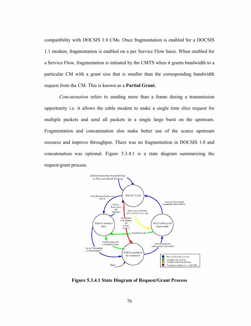
76
compatibility with DOCSIS 1.0 CMs. Once fragmentation is enabled for a DOCSIS
1.1 modem, fragmentation is enabled on a per Service Flow basis. When enabled for
a Service Flow, fragmentation is initiated by the CMTS when it grants bandwidth to a
particular CM with a grant size that is smaller than the corresponding bandwidth
request from the CM. This is known as a Partial Grant.
Concatenation refers to sending more than a frame during a transmission
opportunity i.e. it allows the cable modem to make a single time slice request for
multiple packets and send all packets in a single large burst on the upstream.
Fragmentation and concatenation also make better use of the scarce upstream
resource and improve throughput. There was no fragmentation in DOCSIS 1.0 and
concatenation was optional. Figure 5.3.4.1 is a state diagram summarizing the
request/grant process.
Figure 5.3.4.1 State Diagram of Request/Grant Process
77
5.4 OPNET’s DOCSIS Models
OPNET's Model Library is recognized industry-wide as the most advanced
suite of models of network protocols, technologies, and applications available.
OPNET's DOCSIS model suite has been developed jointly by OPNET and the
CableLabs' Bandwidth Modeling and Management Vendor Forum. The model is
based on the DOCSIS 1.1 specification (as established by CableLabs), and includes
features relevant to both DOCSIS 1.1 and 1.0 system. The model enables testing
configurations and architectures before building expensive prototypes. It also allows
creation of virtual representations of proposed cable modem networks so as to
evaluate the capacity and quality of service (QoS) characteristics of alternative
designs. A detailed description on OPNET’s DOCSIS model suite can be found in
[21].
5.4.1 Bugs
In the course of performing the different simulations a few bugs were found
out in OPNET’s DOCSIS 1.1 implementation. The first three have been fixed in
OPNET Model Release 9. The last one is yet to be fixed.
• DOCSIS RTP process does not add unicast requests to the MAP in the
required intervals .The docsis_cmts process calls the RTP process to find out
whether or not a unicast request should be added to the MAP every time it
creates a new MAP. The RTP process should be basically checking whether
the time since the last poll is greater than the real-time polling interval or not.
78
If yes, a unicast request must be added to the MAP. There seems to be a
logical error due to which this is not happening. As a result performance
studies were not done with the rtPS QoS class.
• CMTS does not add Pending Grant IEs to the MAP. When the CMTS
identifies that it can't satisfy a grant, it has to add a Pending IE to the MAP to
inform the CM that it’s request has been received and that it would be
satisfied in the subsequent MAP. This does not happen, due to a bug in the
implementation. This results in the CM contending again which it wouldn't
have done had the pending grant IE been added to the MAP. This would have
a small but definite impact on the results obtained. The fact that the CMs
contend again would have led to an increase in the number of contentions and
hence the collision probability. But this is true only for the experiments for
which concatenation and fragmentation had been disabled, because if
fragmentation had been enabled, the CMTS does not deny a grant, but instead
gives a partial grant. This bug may have had some effect on the simulation
results.
• DOCSIS nrtPS does not add unicast requests to the MAP. DOCSIS 1.1 offers
unicast request opportunities to nrtPS to avoid contention during times of
network contention. But due to a logical bug in the implementation, the
CMTS was not adding the unicast request polls to the MAP. This is the only
feature that differentiates nrtPS from BE. Again because of this we were not
able conduct performance studies with nrtPS.
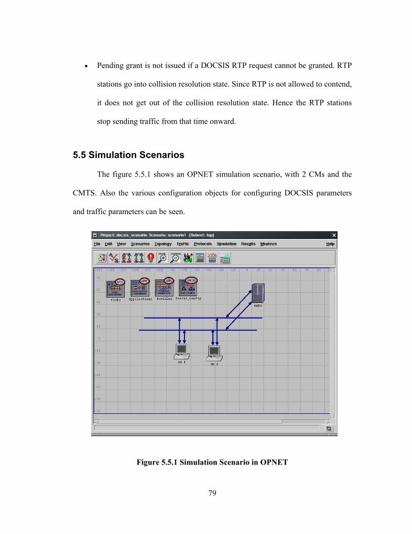
79
• Pending grant is not issued if a DOCSIS RTP request cannot be granted. RTP
stations go into collision resolution state. Since RTP is not allowed to contend,
it does not get out of the collision resolution state. Hence the RTP stations
stop sending traffic from that time onward.
5.5 Simulation Scenarios
The figure 5.5.1 shows an OPNET simulation scenario, with 2 CMs and the
CMTS. Also the various configuration objects for configuring DOCSIS parameters
and traffic parameters can be seen.
`
Figure 5.5.1 Simulation Scenario in OPNET
80
5.6 Performance Evaluation of DOCSIS 1.1 QoS
5.6.1 DOCSIS CMTS Parameters
Physical Media Profile:
This defines profiles that allow the user to configure the RF specifications
(modulation, channel width, data rate, and center frequency) and interleave
latency of downstream channels and upstream channels. Parameters used for
these simulations were:
Upstream Bandwidth: 640 Kb/s
Downstream bandwidth: 27Mb/s
Upstream modulation scheme: QPSK
Downstream modulation scheme: 64 QAM
MAP Profile:
This attribute defines the bandwidth allocation MAP profiles that are applied
to the upstream channel parameters on CMTS nodes.
MAP inter-arrival time: 0.2s
Short data grant limit: 128 bytes
Long data grant limit: 10000 bytes
Data back off start: 7
Data back off end: 16
Number of contention slots: 64
Bytes per minislot: 4 bytes
81
5.6.2 Experiment 1 a. Comparison of Best Effort & UGS Delays b. Effect of Piggybacking on Best Effort Delay Configuring the UGS station:
The total upstream bandwidth is 640Kbps. 64 minislots have been allotted for
contention. The remaining bandwidth can be calculated in the following way:
Duration of one minislot = 50 us
Number of minislots in MAP: MAP time / Duration of one minislot
= 0.2/0.00005
= 4000 minislots
Number of minislots available
for data transmission = 4000- (32+2) [2 slots for station maintenance]
Size of one minislot = 4 bytes
Remaining bandwidth = (3966 * 4 * 8) / 0.2
= 634.56 Kbps
Of the remaining bandwidth ~ 10% has been allotted to UGS. Since UGS is generally
used for Constant Bit Rate Traffic, i.e. for flows that generate fixed packets in regular
intervals, the station has been configured in the following manner.
UGS Station Traffic Statistics:
Request Packet size = 1000 bytes
Packet Inter-arrival time = 0.21s
Packet size distribution: Constant
Inter-arrival times distribution: Constant

82
UGS QoS Parameters:
The Nominal Grant interval is set so that there is a grant every MAP and it is
also approximately equal to the packet inter-arrival time.
Grant Size = 1300 bytes
Nominal Grant Interval = 0.2s
Physical overhead calculation:
The following parameters are used for the physical overhead calculation.
These are configured as a part of the Physical Media Overhead within the MAP
Profiles. Messages can be short or long data frames. Short data frames have a 100-
byte limit while long frames can go up to 10,000 bytes. Since all the packets lengths
used in the simulation exceeds 100 bytes, the long data frame physical parameters are
listed below. Before transmitting a packet received from the higher layer, the CMTS
divides the packet into code words. It then adds FEC error correction bytes to each
code word and preamble length bits to each frame.
Preamble Length: 56 bits
FEC Error Correction (FEC Parity): 16 bytes
FEC Code Word Length: 226 bytes
Guard Time (bits): 40
Last Code Word Mode: Fixed
A sample overhead calculation for a packet size of 1300 bytes is shown below.
The MAC headers are added to the IP frame (includes 20 bytes of IP header and 20
bytes of TCP header).
83
Total message size before upstream physical overhead is added = Size of IP frame +
DOCSIS_MSG_PDU_HDR_SIZE (20 bytes)
Message size = Payload size + TCP/IP headers + MAC Overhead
= 1300 + 40 + 20
= 1360 bytes
No of code words = (message size)/(FEC Code word length- FEC Parity)
= 1360 /(226-16)
= 6.47
= 7 (rounded off to the highest integer)
Now the final message size = number of code words x FEC code word
= 7 x 226
= 1582
Total Frame Size = Message size + (Preamble + Guard Time)/8
= 1582 + (56 + 40)/8
= 1582 + 12
= 1594 bytes.
The total bandwidth allocated to the UGS station is (1594 * 8)/0.2 =63.76 Kbps.
Configuring the BE stations:
The rest of the bandwidth was distributed among the BE stations. The stations
had identical parameters and also traffic statistics. The load was increased by adding
stations. Fragmentation and concatenation were disabled.
BE Stations Traffic Statistics:
Mean packet Size = 800 bytes
Mean packet inter-arrival time = 0.22s
Packet size distribution: Exponential
Inter-arrival time distribution: Exponential
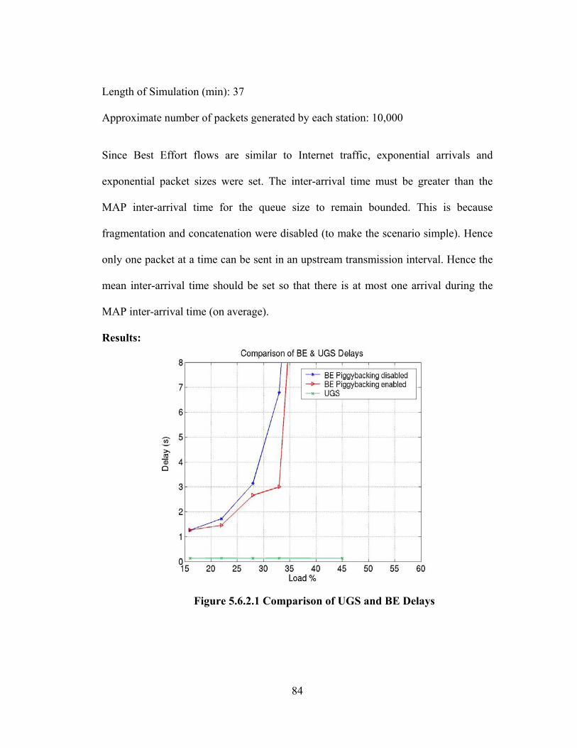
84
Length of Simulation (min): 37
Approximate number of packets generated by each station: 10,000
Since Best Effort flows are similar to Internet traffic, exponential arrivals and
exponential packet sizes were set. The inter-arrival time must be greater than the
MAP inter-arrival time for the queue size to remain bounded. This is because
fragmentation and concatenation were disabled (to make the scenario simple). Hence
only one packet at a time can be sent in an upstream transmission interval. Hence the
mean inter-arrival time should be set so that there is at most one arrival during the
MAP inter-arrival time (on average).
Results:
Figure 5.6.2.1 Comparison of UGS and BE Delays
85
Analysis:
The performance of BE traffic was compared with UGS. UGS flows are
allowed to reserve a certain portion of the bandwidth. No requests for transmission
are needed; hence UGS has a low bounded constant delay, since it receives a grant
every MAP and thus queue size is low and bounded. BE on the other hand has
“request grant, request grant” pattern. Stations have to contend for sending requests
and have to wait for grants in the subsequent MAPs. Contentions may result in
collision and thus there may be increased delay due to retransmissions. The effect of
piggybacking on delay is also studied. With piggybacking enabled, requests are
piggybacked to outgoing data and thus the frequency of contention is reduced and
delay is reduced. We see that the system saturates quickly. This is because
fragmentation and concatenation were disabled; hence only one frame can be sent per
MAP. This leads to relatively high delay values, since the queue size builds up
quickly. This is because as load increases, the CMTS would not be able to satisfy all
the requests from all the stations. Also in this experiment and in all the experiments
that follow, the load value is the actual load value and not the calculated value. The
load value was calculated from the simulations as
Reserved slot time in MAP/ Total MAP duration. We report actual loads because with
the exponential packet lengths and exponential inter-arrival times, it is very difficult
to predict the load values from the mean packet size and inter-arrival time. The packet
lengths are exponentially distributed and hence they would be distributed in a wide
86
range of values. Also, as explained before, there is also some amount of complexity
involved in the computation of the upstream physical overhead.
5.6.3 Experiment 2
Effect of Fragmentation & Concatenation
Configuring the UGS station:
As before ~ 10% of the total bandwidth was allotted to the UGS Station. The
MAP configuration parameters were retained for all the experiments.
UGS Station Traffic Statistics:
Request Packet size = 1000 bytes
Packet Inter-arrival time = 0.21s
Packet size distribution: Constant
Inter-arrival times distribution: Constant
Number of packets generated by each station: 10,000
UGS QoS Parameters:
Grant Size = 1300 bytes
Nominal Grant Interval = 0.2s
The total bandwidth allocated to the UGS station is (1594 * 8)/0.2 =63.76 Kbps.
Configuring the BE stations:
The rest of the bandwidth was distributed among the 11 BE stations. The
stations had identical parameters and also traffic statistics. The load was increased by
adding stations to the scenario. The experiment was performed to study the effect of
fragmentation and concatenation on performance i.e., on mean delay. Hence one set
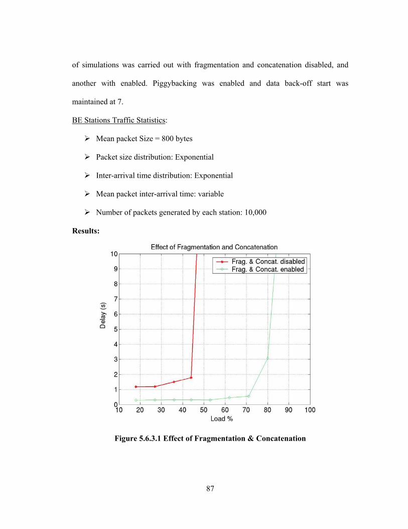
87
of simulations was carried out with fragmentation and concatenation disabled, and
another with enabled. Piggybacking was enabled and data back-off start was
maintained at 7.
BE Stations Traffic Statistics:
Mean packet Size = 800 bytes
Packet size distribution: Exponential
Inter-arrival time distribution: Exponential
Mean packet inter-arrival time: variable
Number of packets generated by each station: 10,000
Results:
Figure 5.6.3.1 Effect of Fragmentation & Concatenation
88
Analysis:
DOCSIS concatenation combines multiple upstream packets into one packet
to reduce packet overhead (as explained already, the physical upstream overhead is
considerable) and overall latency, and to increase transmission efficiency. Using
concatenation, a DOCSIS cable modem makes only one bandwidth request for
multiple packets, as opposed to making a different bandwidth request for each
individual packet; this technique is especially effective for bursty real-time traffic,
such as voice calls. Since a single bandwidth request is made for a multiple frames,
the queuing time is reduced, and this brings down the overall access delay. This also
saves upstream bandwidth to an extent since sending of many small request packets is
avoided. The need for frequent contention is also reduced, resulting in fewer
collisions. This also contributes to an improvement in performance. When enabling
concatenation, fragmentation should also be enabled; otherwise packets that are too
large for transmission in a single MAP are not transmitted. That is, when
concatenation is enabled the request sizes are generally big, and the CMTS does not
issue a grant at all if fragmentation is disabled and there are not enough minislots in
the current MAP. Thus fragmentation and concatenation together help in better
utilization of the upstream bandwidth compared to the case when both were disabled.
In that case we are only able to reach loads of 45%, since after that the queue builds
up and delay increases indefinitely. But when fragmentation and concatenation were
enabled, we are able to reach much higher load values with lesser access delays.
89
5.6.4 Experiment 3 Effect of Backoff Start and Piggybacking Configuring the UGS station
As before ~ 10% of the total bandwidth was allotted to the UGS Station. The
MAP configuration parameters were retained for all the experiments.
UGS Station Traffic Statistics:
Request Packet size = 1000 bytes
Packet Inter-arrival time = 0.21s
Packet size distribution: Constant
Inter-arrival times distribution: Constant
Number of packets generated by each station: 10,000
UGS QoS Parameters:
Grant Size = 1300 bytes
Nominal Grant Interval = 0.2s
The total bandwidth allocated to the UGS station is (1594 * 8)/0.2 =63.76
Kbps.
Configuring the BE stations:
The rest of the bandwidth was distributed among the BE stations. The stations
had identical parameters and also traffic statistics. In this experiment the number of
BE stations were maintained constant at 11 and the load was changed by changing the
inter-arrival times. In order to make load values predictable and to simplify protocol
operation, fragmentation and concatenation were disabled and packet lengths were
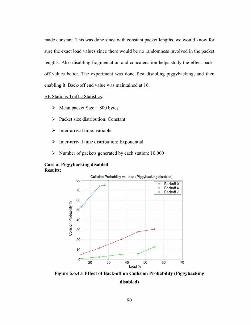
90
made constant. This was done since with constant packet lengths, we would know for
sure the exact load values since there would be no randomness involved in the packet
lengths. Also disabling fragmentation and concatenation helps study the effect back-
off values better. The experiment was done first disabling piggybacking, and then
enabling it. Back-off end value was maintained at 16.
BE Stations Traffic Statistics:
Mean packet Size = 800 bytes
Packet size distribution: Constant
Inter-arrival time: variable
Inter-arrival time distribution: Exponential
Number of packets generated by each station: 10,000
Case a: Piggybacking disabled Results:
Figure 5.6.4.1 Effect of Back-off on Collision Probability (Piggybacking
disabled)
91
Analysis:
We see the effect of the data back-off start value on collision probability. For
a data back-off of zero we see that the collision probability is very high and it
increases with increase in load. This is because since the initial value is zero, the
back-off window is zero (no random wait). Hence the probability that two stations
would pick the same minislot for contention is very high. This would result in a
collision and the contention requests of both the stations would be lost. Also since
piggybacking has been disabled, there are more frequent contentions as load
increases. This leads to increased probability of collisions. We see that the collision
probability decreases as the back-off value increases. This is because the station
defers its transmission by a greater number of minislots (since its window size is big).
Also we see that we are able to go up to much higher loads for back-off 4 & 7. This is
because with a lower back-off value, there would be increased number of
retransmissions since the collision probability is more. Hence the queue builds up
quickly. But with greater back-off values, the collision probability is comparatively
less and hence we are able to go up to comparatively high load values.
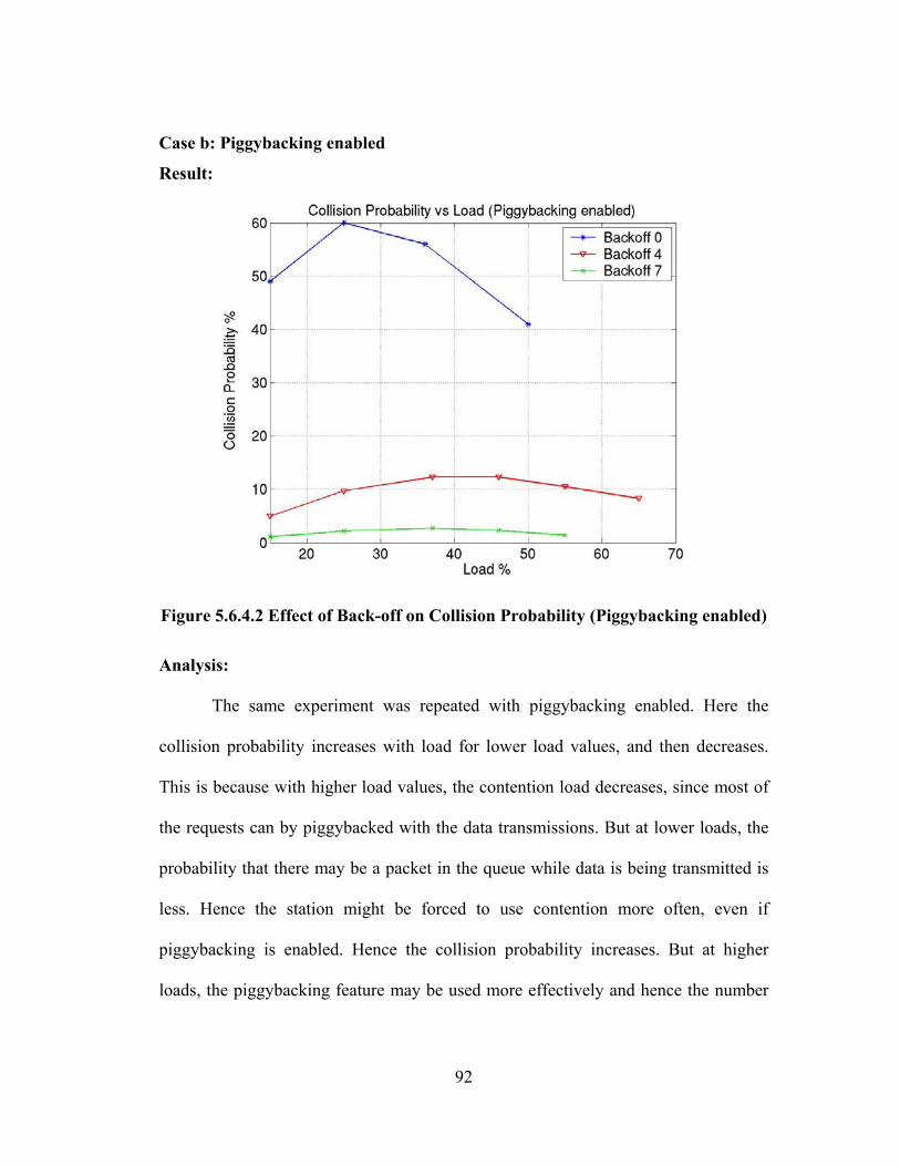
92
Case b: Piggybacking enabled
Result:
Figure 5.6.4.2 Effect of Back-off on Collision Probability (Piggybacking enabled) Analysis:
The same experiment was repeated with piggybacking enabled. Here the
collision probability increases with load for lower load values, and then decreases.
This is because with higher load values, the contention load decreases, since most of
the requests can by piggybacked with the data transmissions. But at lower loads, the
probability that there may be a packet in the queue while data is being transmitted is
less. Hence the station might be forced to use contention more often, even if
piggybacking is enabled. Hence the collision probability increases. But at higher
loads, the piggybacking feature may be used more effectively and hence the number
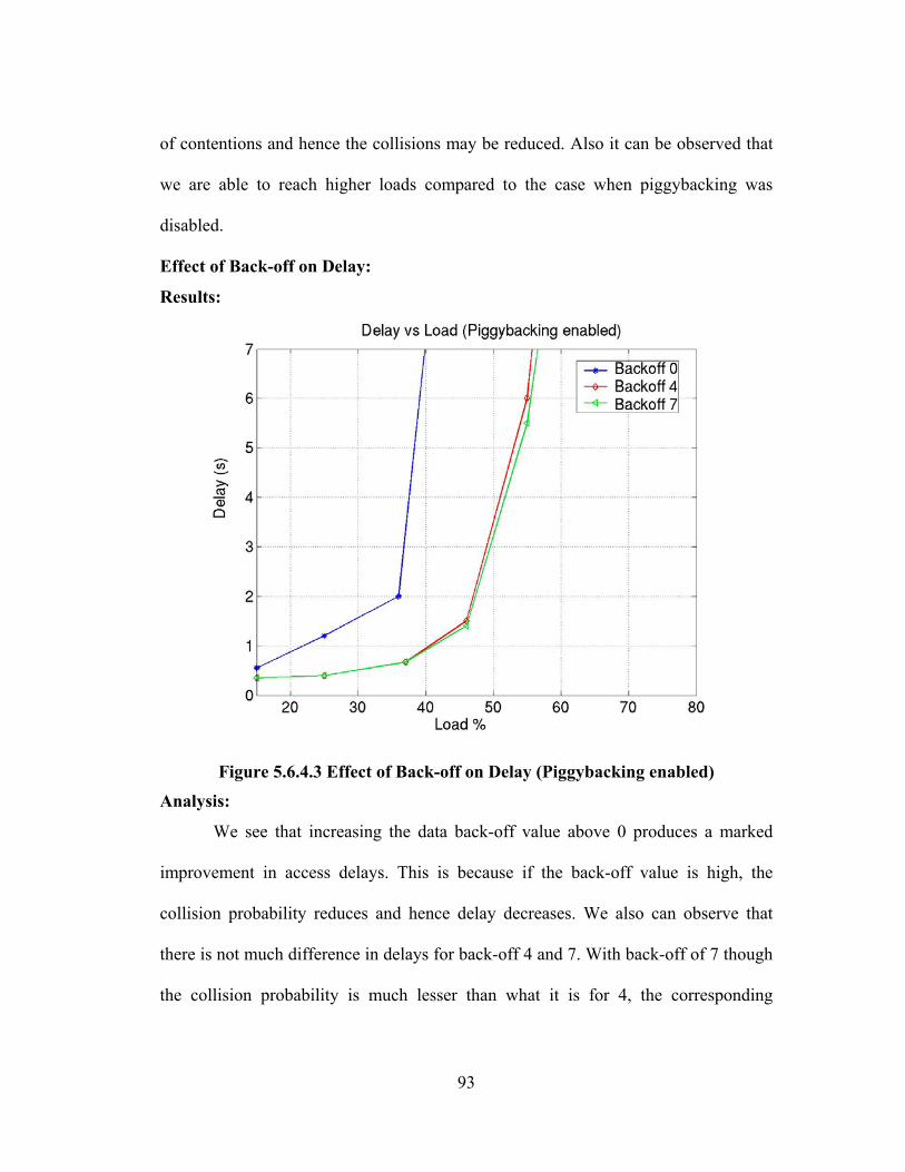
93
of contentions and hence the collisions may be reduced. Also it can be observed that
we are able to reach higher loads compared to the case when piggybacking was
disabled.
Effect of Back-off on Delay:
Results:
Figure 5.6.4.3 Effect of Back-off on Delay (Piggybacking enabled)
Analysis:
We see that increasing the data back-off value above 0 produces a marked
improvement in access delays. This is because if the back-off value is high, the
collision probability reduces and hence delay decreases. We also can observe that
there is not much difference in delays for back-off 4 and 7. With back-off of 7 though
the collision probability is much lesser than what it is for 4, the corresponding
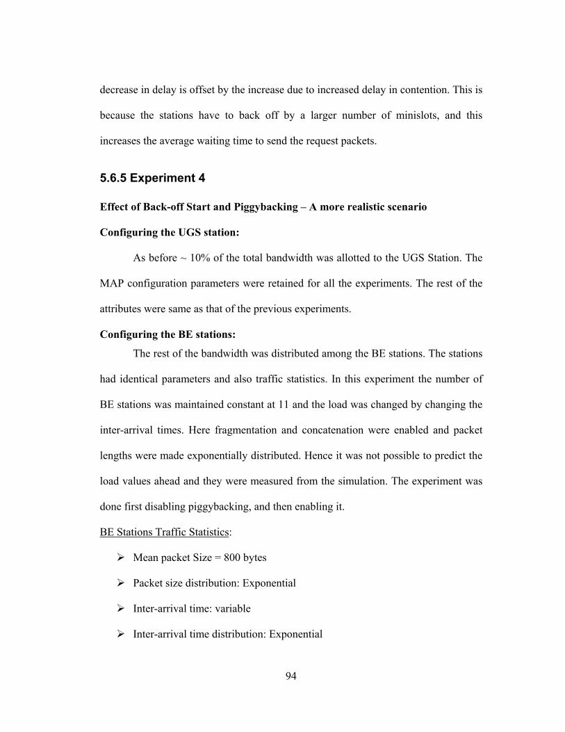
94
decrease in delay is offset by the increase due to increased delay in contention. This is
because the stations have to back off by a larger number of minislots, and this
increases the average waiting time to send the request packets.
5.6.5 Experiment 4 Effect of Back-off Start and Piggybacking – A more realistic scenario Configuring the UGS station:
As before ~ 10% of the total bandwidth was allotted to the UGS Station. The
MAP configuration parameters were retained for all the experiments. The rest of the
attributes were same as that of the previous experiments.
Configuring the BE stations:
The rest of the bandwidth was distributed among the BE stations. The stations
had identical parameters and also traffic statistics. In this experiment the number of
BE stations was maintained constant at 11 and the load was changed by changing the
inter-arrival times. Here fragmentation and concatenation were enabled and packet
lengths were made exponentially distributed. Hence it was not possible to predict the
load values ahead and they were measured from the simulation. The experiment was
done first disabling piggybacking, and then enabling it.
BE Stations Traffic Statistics:
Mean packet Size = 800 bytes
Packet size distribution: Exponential
Inter-arrival time: variable
Inter-arrival time distribution: Exponential
95
Number of packets generated by each station: 10,000
Results:
Figure 5.6.5.1 Effect of Piggybacking on Collision Probability
Analysis:
The simulations were carried out to study the effect of back-off on collision
probability, for back-offs 0, 4 & 7. The results are plotted in figure 5.6.5.1 showing
the effect of piggybacking for back-off 4. We see that enabling piggybacking has
reduced the collision probability since the need for contention is reduced with
piggybacking enabled. But we see that the trend is same whether piggybacking has
been enabled or not. This is because concatenation has been enabled. So the effect of
concatenation is more prominent. Since with concatenation enabled, requests for
multiple frames can be made, there is less need for contention. Hence the collision
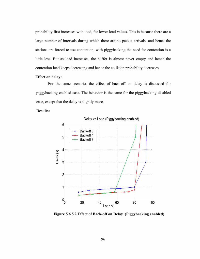
96
probability first increases with load, for lower load values. This is because there are a
large number of intervals during which there are no packet arrivals, and hence the
stations are forced to use contention; with piggybacking the need for contention is a
little less. But as load increases, the buffer is almost never empty and hence the
contention load keeps decreasing and hence the collision probability decreases.
Effect on delay:
For the same scenario, the effect of back-off on delay is discussed for
piggybacking enabled case. The behavior is the same for the piggybacking disabled
case, except that the delay is slightly more.
Results:
Figure 5.6.5.2 Effect of Back-off on Delay (Piggybacking enabled)
97
Analysis:
For low loads, increasing the back-off value reduces the collision probability
and hence delay decreases significantly due to reduced retransmissions. There is not
much of a difference between back-off 7 and 4 for lower loads, since the decrease in
delay as a consequence of decreased collision is offset by the increased delay incurred
during contention. This is because as the back-off value is more, the back-off window
is larger and hence the station defers by a greater number of minislots before
transmitting its request. This increases delay since for a specified value of priority,
the CMTS issues grants in the order in which they were received. But it is observed
that the load value at which the system saturates, i.e. the buffer builds up, decreases
as the back-off value increases. This is because each station defers its transmission by
a greater number of minislots, and hence it is possible that the request may not reach
the CMTS before the next MAP is transmitted. Hence it may so happen that the
station is forced to wait for two MAP periods. This leads to the queue building up and
delay rising indefinitely. But for back-off zero, the window starts with a small value
and slowly increases each time a collision occurs and hence it is more adaptive to the
load, and helps utilizing the entire bandwidth.
Comparing the results illustrated in figure 5.6.5.2 with those in figure 5.6.4.3,
we see that the system saturates quickly for higher back-off values in figure 5.6.5.2,
as opposed to figure 5.6.4.3. This is because for the experiment of figure 5.6.5.2,
fragmentation and concatenation were enabled, whereas for experiment 3 (figure
5.6.4.3) both were disabled. So with fragmentation and concatenation enabled, it is
98
possible to achieve a much higher throughput and utilize the entire bandwidth
available in one MAP period. Also if the back off is high, with the piggybacking
enabled, it is possible that certain requests reach the CMTS only after the subsequent
MAP is sent. This leads to an increased waiting time, and also building up of the
queue. On the other hand, with the previous experiment (figure 5.6.4.3), since
fragmentation and concatenation were disabled, the collisions had a prominent effect
and it wouldn’t be possible to saturate the entire available bandwidth. So the system
saturates quickly for the lower back-off value.
5.6.6 Experiment 5 Effect of Priorities on Delay Simulation Scenario:
The set up consisted of 2 UGS stations and 8 Best Effort stations. The packet
attributes and other UGS parameters were the same as that of previous experiments.
The total bandwidth allocated to the UGS station is (1594 * 8 *2)/0.2 = 127.72 Kbps.
There were 8 Best Effort stations with priorities [0-3], i.e. 2 stations per priority. The
number of stations was maintained constant throughout the experiment. Load was
changed by changing the packet inter-arrival times. Since fragmentation and
concatenation were enabled, there was no constraint on the inter-arrival times (i.e.
they are no longer required to be greater than the MAP duration.). Again load values
were measured from the simulation.
BE Stations Traffic Statistics:
Mean packet Size = 800 bytes
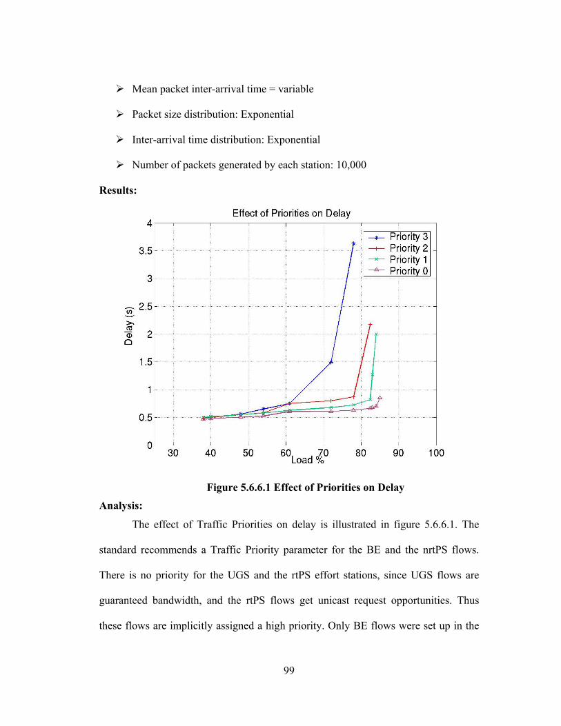
99
Mean packet inter-arrival time = variable
Packet size distribution: Exponential
Inter-arrival time distribution: Exponential
Number of packets generated by each station: 10,000
Results:
Figure 5.6.6.1 Effect of Priorities on Delay
Analysis:
The effect of Traffic Priorities on delay is illustrated in figure 5.6.6.1. The
standard recommends a Traffic Priority parameter for the BE and the nrtPS flows.
There is no priority for the UGS and the rtPS effort stations, since UGS flows are
guaranteed bandwidth, and the rtPS flows get unicast request opportunities. Thus
these flows are implicitly assigned a high priority. Only BE flows were set up in the
100
simulation experiment for studying the effect of priorities. The CMTS uses the
Traffic Priority attribute for determining precedence in grant generation. Priorities do
not affect contention process, though. Traffic Priorities range from 0-7 applicable to
BE and nrtPS, 0 being the highest. It is clearly seen that the higher priority stations
have lower access delay, since it is given preference in transmitting data. The grants
in the MAP are scheduled in order of priority, and thus a high priority station gets to
transmit its packets first and thus suffers lower access delays.
101
6 Conclusions and Future Work
We finish up this thesis with a quick summary of the contributions of this
research effort and a few pointers to future work
6.1 Summary of Contributions • Characterized the performance of HF2Q: The performance of a new queuing
mechanism was characterized completely. The properties of HF2Q were
studied from simulations under different load conditions. The performance was
evaluated by studying the delay and throughput characteristics of the queuing
algorithm.
• Compared the performance of HF2Q to WFQ: The performance of HF2Q
was compared to that of WFQ since HF2Q results from a modification made to
WFQ. The comparisons were made under different scenarios (different
combinations of reservations and incoming load for the different flows). This
helps us better understand the behavior of both the algorithms, which are
extremely complicated.
• Evaluated the performance of QoS features of DOCSIS 1.1: This is very
significant because a complete performance evaluation of this particular
standard (standardized in 2001) has never been done before. DOCSIS is a very
complex MAC protocol with a number of new QoS features introduced. Hence
understanding of the operation of the protocol and evaluating the performance
of the QoS features for different classes of traffic is very important for any
102
future work. This thesis has evaluated the QoS features for 2 classes of traffic
namely UGS and Best Effort.
6.2 Summary of Conclusions • It was determined from simulations that HF2Q behaved as FIFO when the total
system load is less than unity and behaves as WFQ when the total system load
exceeds unity.
• The throughput behavior of HF2Q was studied and comparisons were made
with that of WFQ and FIFO. Since all three are work-conserving, when the
total load is less than 1, they have identical throughput characteristics. When
the system is overloaded, WFQ and HF2Q behave identically and offer
protection to well-behaving flows, but FIFO essentially offers throughput
according to demand, as expected.
• As regards the performance evaluation of DOCSIS 1.1, it was established from
simulations that the UGS traffic (Constant Bit Rate Traffic) has bounded and
low delays irrespective of the load offered by the other classes. It was also
determined that fragmentation and concatenation improves the delay
characteristics of best effort traffic when the load is very high. Also
piggybacking improves delay for best effort since it reduces the probability of
collision.
103
6.3 Future Work
• There is much scope for future work with regard to the performance of HF2Q.
Understanding how the queuing algorithm behaves is very important because
this could be a significant step in presenting an analytic explanation as to why
HF2Q behaves as FIFO in an underloaded case. This is again another key step
to a possible future work as - finding a closed form expression for the main
waiting time for WFQ.
• DOCSIS 1.1 mentions two other traffic classes namely RTPS and NRTPS. The
evaluation of the performance of these traffic classes was not possible due the
fact that there were bugs in the software implementation. Hence evaluating that
would definitely be an interesting and worthwhile research. Also it would be
interesting to compare the performances of existing scheduling architectures
for DOCSIS 1.1 to the new scheduling architecture proposed in [19].
104
References
[1] Mohammed Hawa, "Stochastic Evaluation of Fair Scheduling with
Applications to Quality-Of-Service in Broadband Wireless Access Networks,”
Ph.D. Dissertation, University of Kansas, August 2003
[2] H. Zhang, “Service disciplines for guaranteed performance service in packet
switching networks,” Proceedings of the IEEE, 83(10): 1374–1399, October
1995.
[3] A. Demers, S. Keshav, and S. Shenker, “Analysis and simulation of a fair
queuing algorithm,” In Journal of Internetworking Research and Experience,
pages 3–26, October 1990. Also in Proceedings of ACM SIGCOMM’89, pp
312.
[4] J. Nagle, On Packet Switches with Infinite Storage, IEEE Transactions on
Communications, Volume 35, pp 435-438, 1987.
[5] L. Zhang, “Virtual Clock: A new traffic control algorithm for packet
switching networks,” In Proceedings of ACM SIGCOMM’90, pages 19-29,
Philadelphia, PA September 1990.
[6] A. Parekh and R. Gallager, “A generalized processor sharing approach to flow
control -the single node case,” In Proceedings of the INFOCOM’92, 1992.
[7] L. Kleinrock, Queuing Systems. John Wiley and Sons, 1975.
[8] A. Parekh, “A Generalized Processor Sharing Approach to Flow Control in
Integrated Services Networks,” PhD dissertation, MIT, February 1992.
105
[9] J. C. R. Bennett and H. Zhang, “WF2Q: Worst-case Fair Weighted Fair
Queueing,” Proceedings of INFOCOM ’96, pp. 120–128, March 1996.
[10] S. J. Golestani, “A Self-Clocked Fair Queueing Scheme for Broadband
Applications,” Proceeding of INFOCOM ’94, pp. 636–646, April 1994.
[11] J. Davin and A. Heybey, “A simulation study of fair queuing and policy
enforcement,” Computer Communication Review, 20(5): 23-29, October 1990.
[12] S. Floyd and V. Jacobson, “Link-sharing and resource management models
for packet networks,” IEEE/ACM Transactions on Networking, 3(4): 365–
386, August 1995.
[13] J.C.R. Bennett and H. Zhang, “Hierarchical packet fair queueing algorithms,”
In Proceedings of the ACMSIGCOMM 96, pages 143–156, Palo Alto, CA,
August 1996.
[14] D. Ferrari, “Real-time communication in an internetwork,” Journal of High
Speed Networks, 1(1): 79-103, 1992.
[15] C. Liu, J. Layland, “Scheduling Algorithms for Multiprogramming in a Hard
RealTime Environment,” Journal of ACM, January 1973
[16] IEEE 802.16 Standard, IEEE Draft Standard for Local and Metropolitan Area
Networks - Part 16: Air Interface for Fixed Broadband Wireless Access
Systems, IEEE Draft P802.16/D5,
http://grouper.ieee.org/groups/802/16/published.html.
[17] Data-Over-Cable Service Interface Specifications, Radio Frequency Interface
Specification, SP-RFIv1.1-I07-010829, http://www.cablemodem.com/.
106
[18] K. Sriram, “Performance of MAC Protocols for Broadband HFC and Wireless
Access Networks,” Advances in Performance Analysis, Vo1. 1, No. 1, pp. 1–
37, 1998.
[19] Mohammed Hawa and David W. Petr, "Quality of Service Scheduling in
Cable and Broadband Wireless Access Systems," Tenth International
Workshop on Quality of Service (IWQoS 2002), pp. 247-255, May 2002.
[20] Todd Lizambri, Fernando Duran and Shukri Wakid, “Priority Scheduling and
Buffer Management for ATM Traffic Shaping,”
http://w3.antd.nist.gov/Hsntg/publications/Papers/lizambri_1299.pdf
[21] Gayathri Chandrasekaran, Mohammed Hawa, David Petr, “Preliminary
Performance Evaluation of QoS in DOCSIS 1.1,” Technical Report ITTC-
FY2003-TR-22736-01, Jan. 2003.
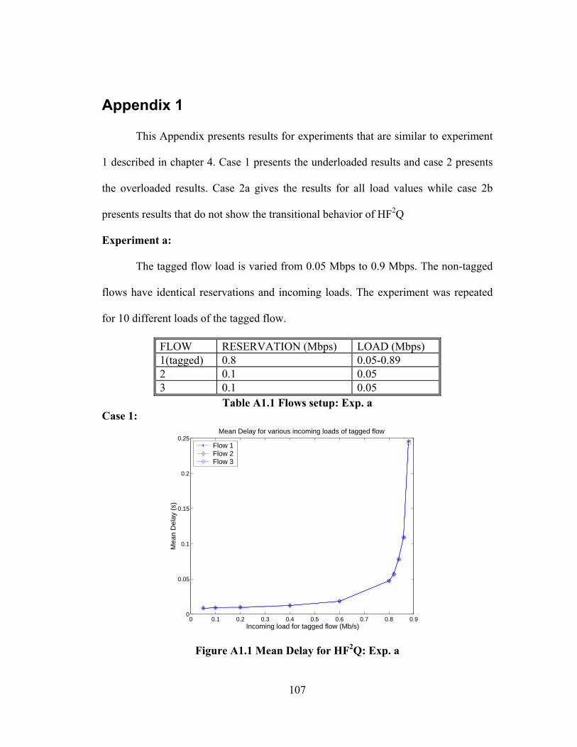
107
Appendix 1
This Appendix presents results for experiments that are similar to experiment
1 described in chapter 4. Case 1 presents the underloaded results and case 2 presents
the overloaded results. Case 2a gives the results for all load values while case 2b
presents results that do not show the transitional behavior of HF2Q
Experiment a:
The tagged flow load is varied from 0.05 Mbps to 0.9 Mbps. The non-tagged
flows have identical reservations and incoming loads. The experiment was repeated
for 10 different loads of the tagged flow.
FLOW RESERVATION (Mbps) LOAD (Mbps) 1(tagged) 0.8 0.05-0.89 2 0.1 0.05 3 0.1 0.05
Table A1.1 Flows setup: Exp. a Case 1:
0 0.1 0.2 0.3 0.4 0.5 0.6 0.7 0.8 0.90
0.05
0.1
0.15
0.2
0.25Mean Delay for various incoming loads of tagged flow
Incoming load for tagged flow (Mb/s)
Mea
n D
elay
(s)
Flow 1Flow 2Flow 3
Figure A1.1 Mean Delay for HF2Q: Exp. a

108
0 0.1 0.2 0.3 0.4 0.5 0.6 0.7 0.8 0.90
0.05
0.1
0.15
0.2
0.25Mean Delay for various incoming loads of tagged flow
Incoming load for tagged flow (Mb/s)
Mea
n D
elay
(s)
Flow 1Flow 2Flow 3
Figure A1.2 Mean Delay for WFQ: Exp. a
Case 2a:
0.9 0.95 1 1.05 1.1 1.150
0.2
0.4
0.6
0.8
1
1.2
1.4Mean Delay for various incoming loads of tagged flow
Incoming load for tagged flow (Mb/s)
Mea
n D
elay
(s)
Flow 1Flow 2
Figure A1.3 Mean Delay for HF2Q: Exp. a
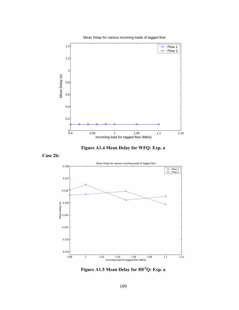
109
0.9 0.95 1 1.05 1.1 1.150
0.2
0.4
0.6
0.8
1
1.2
1.4
Mean Delay for various incoming loads of tagged flow
Incoming load for tagged flow (Mb/s)
Mea
n D
elay
(s)
Flow 1Flow 2
Figure A1.4 Mean Delay for WFQ: Exp. a
Case 2b:
0.98 1 1.02 1.04 1.06 1.08 1.1 1.12
0.101
0.102
0.103
0.104
0.105
0.106
0.107
0.108Mean Delay for various incoming loads of tagged flow
Incoming load for tagged flow (Mb/s)
Mea
n D
elay
(s)
Flow 1Flow 2
Figure A1.5 Mean Delay for HF2Q: Exp. a
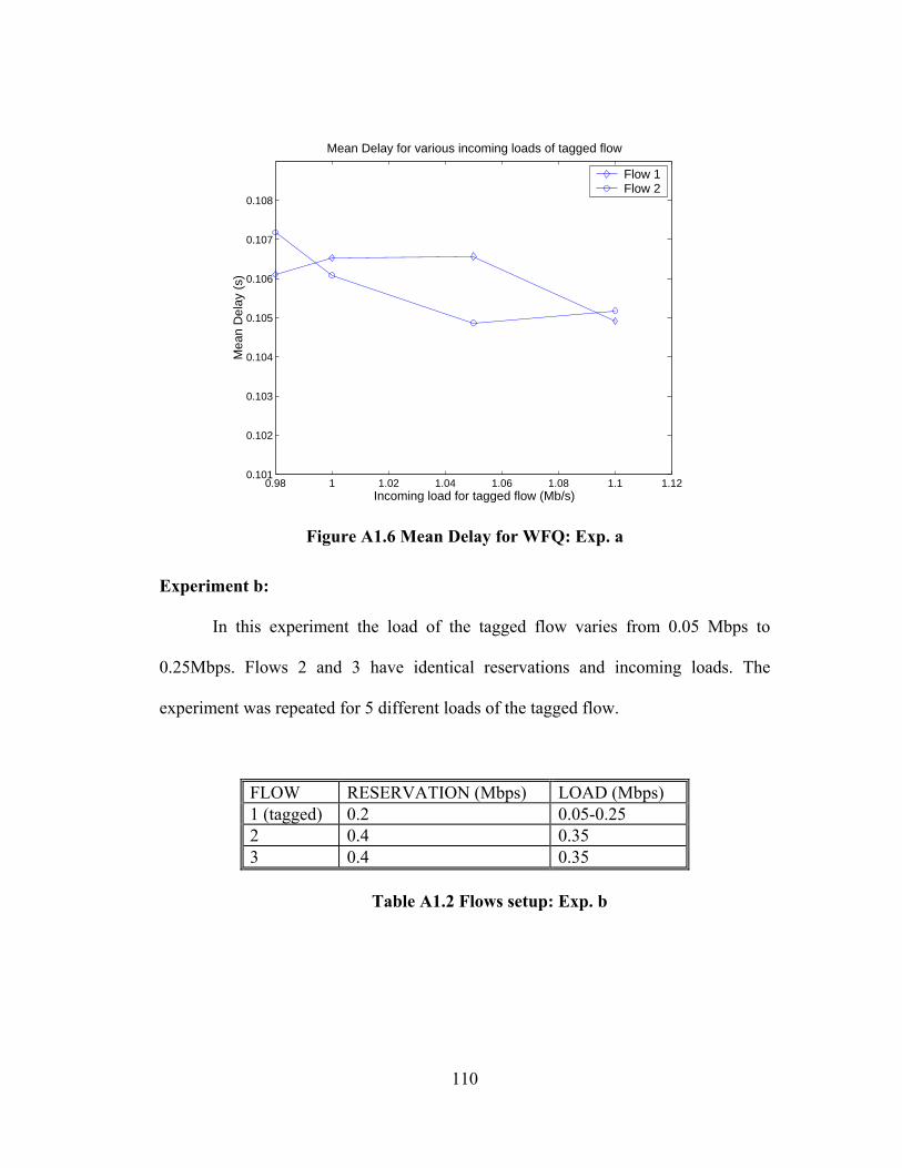
110
0.98 1 1.02 1.04 1.06 1.08 1.1 1.120.101
0.102
0.103
0.104
0.105
0.106
0.107
0.108
Mean Delay for various incoming loads of tagged flow
Incoming load for tagged flow (Mb/s)
Mea
n D
elay
(s)
Flow 1Flow 2
Figure A1.6 Mean Delay for WFQ: Exp. a
Experiment b:
In this experiment the load of the tagged flow varies from 0.05 Mbps to
0.25Mbps. Flows 2 and 3 have identical reservations and incoming loads. The
experiment was repeated for 5 different loads of the tagged flow.
FLOW RESERVATION (Mbps) LOAD (Mbps) 1 (tagged) 0.2 0.05-0.25 2 0.4 0.35 3 0.4 0.35
Table A1.2 Flows setup: Exp. b

111
Case 1:
0.05 0.1 0.15 0.2 0.250
0.05
0.1
0.15
0.2
0.25Mean Delay for various incoming loads of tagged flow
Incoming load for tagged flow (Mb/s)
Mea
n D
elay
(s)
Flow 1Flow 2Flow 3
Figure A1.7. Mean Delay for HF2Q: Exp. b
0.05 0.1 0.15 0.2 0.250
0.05
0.1
0.15
0.2
0.25Mean Delay for various incoming loads of tagged flow
Incoming load for tagged flow (Mb/s)
Mea
n D
elay
(s)
Flow 1Flow 2Flow 3
Figure A1.8 Mean Delay for WFQ: Exp. b
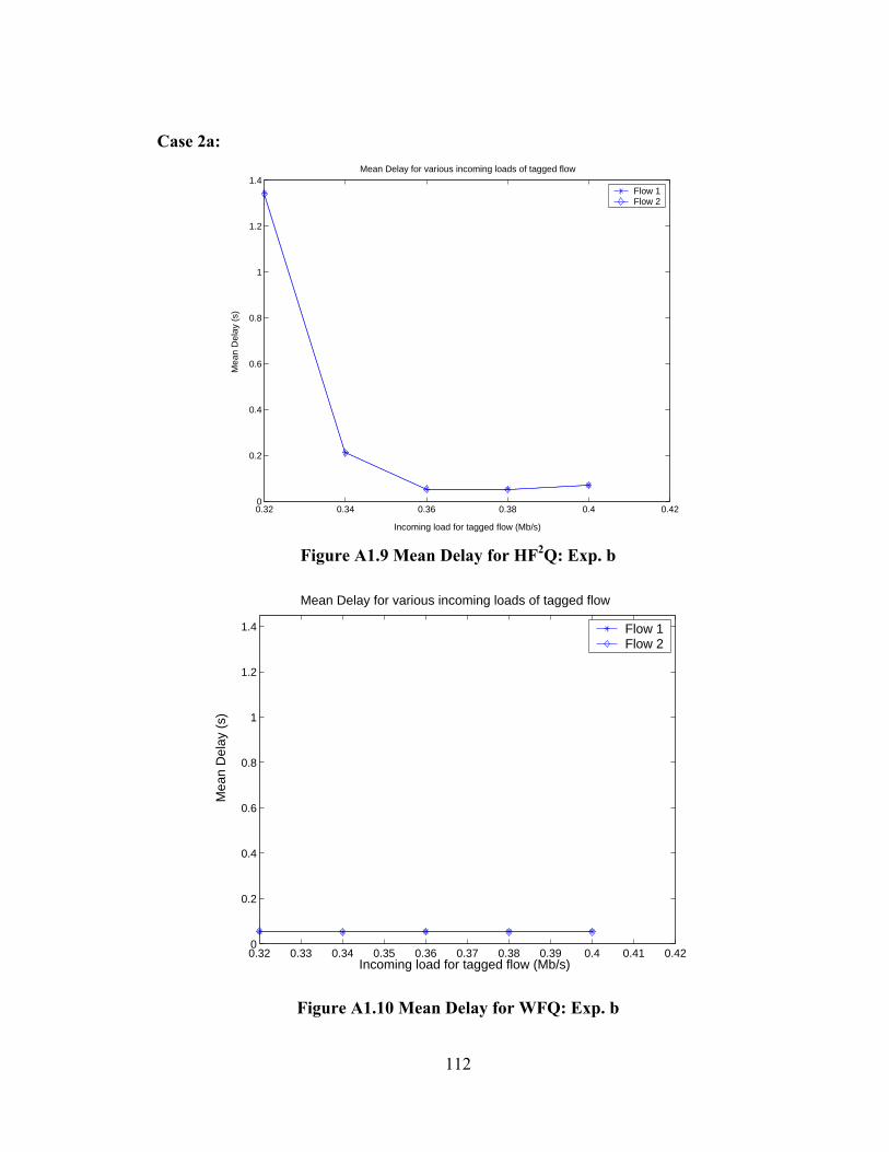
112
Case 2a:
0.32 0.34 0.36 0.38 0.4 0.420
0.2
0.4
0.6
0.8
1
1.2
1.4Mean Delay for various incoming loads of tagged flow
Incoming load for tagged flow (Mb/s)
Mea
n D
elay
(s)
Flow 1Flow 2
Figure A1.9 Mean Delay for HF2Q: Exp. b
0.32 0.33 0.34 0.35 0.36 0.37 0.38 0.39 0.4 0.41 0.420
0.2
0.4
0.6
0.8
1
1.2
1.4
Mean Delay for various incoming loads of tagged flow
Incoming load for tagged flow (Mb/s)
Mea
n D
elay
(s)
Flow 1Flow 2
Figure A1.10 Mean Delay for WFQ: Exp. b
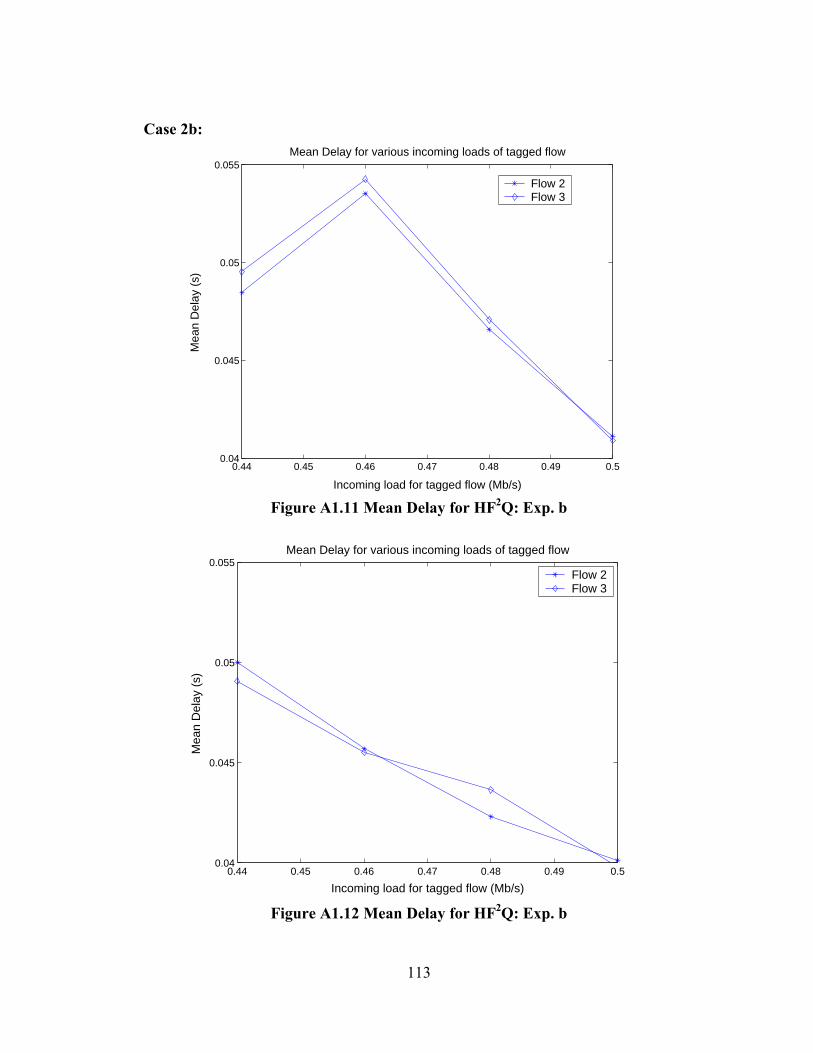
113
Case 2b:
0.44 0.45 0.46 0.47 0.48 0.49 0.50.04
0.045
0.05
0.055Mean Delay for various incoming loads of tagged flow
Incoming load for tagged flow (Mb/s)
Mea
n D
elay
(s)
Flow 2Flow 3
Figure A1.11 Mean Delay for HF2Q: Exp. b
0.44 0.45 0.46 0.47 0.48 0.49 0.50.04
0.045
0.05
0.055Mean Delay for various incoming loads of tagged flow
Incoming load for tagged flow (Mb/s)
Mea
n D
elay
(s)
Flow 2Flow 3
Figure A1.12 Mean Delay for HF2Q: Exp. b