performance improvement of bearingless multi-sector pmsm...
TRANSCRIPT
1
Performance Improvement of BearinglessMulti-Sector PMSM with Optimal Robust Position
ControlG. Valente, IEEE Member, A. Formentini, IEEE Member, L. Papini, C. Gerada, IEEE Member, P. Zanchetta,
IEEE Senior Member
Abstract—Bearingless machines are relatively new devices thatconsent to suspend and spin the rotor at the same time. Theycommonly rely on two independent sets of three-phase windingsto achieve a decoupled torque and suspension force control.Instead, the winding structure of the proposed multi-sectorpermanent magnet (MSPM) bearingless machine permits tocombine the force and torque generation in the same three-phasewinding.In this paper the theoretical principles for the torque andsuspension force generation are described and a referencecurrent calculation strategy is provided. Then, a robust optimalposition controller is synthesized. A Multiple Resonant Controller(MRC) is then integrated in the control scheme in order tosuppress the position oscillations due to different periodic forcedisturbances and enhance the levitation performance. TheLinear-Quadratic Regulator (LQR) combined with the LinearMatrix Inequalities (LMI) theory have been used to obtainthe optimal controller gains that guarantee a good systemrobustness.Simulation and experimental results will be presented to validatethe proposed position controller with a prototype bearinglessMSPM machine.
Index Terms—Bearingless machines, Multi-phase machines,LQR, LMI, H2 control, H∞ control.
I. INTRODUCTION
Bearingless Machines (BMs) embed in a single machinethe features of Active Magnetic Bearings (AMBs) and con-ventional motors. Despite the fact that the first BM has beenpresented in the early ’70 [1], they have not received muchattention till the last couple of decades [2]. This technologyhas become of particular interest for ultra-high speeds drives[3]. It is the case of compressors, spindles, flywheels [4],[5] and generators where high rotational speed operationmeans minimize the weight, size and cost, and maximize theefficiency of the whole system [6]. Furthermore, bearinglessdrives would provide a possible solution for installations inextremely harsh environments, such as vacuum and very low
G. Valente, A. Formentini and P. Zanchetta are with thePEMC group, University of Nottingham, Nottingham, NG7 2RD,UK (e-mail: [email protected], [email protected],[email protected]).
L. Papini and C. Gerada are with the PEMC group, University ofNottingham and University of Nottingham China campus (e-mail: [email protected], [email protected]).
and high temperatures, and in sterile conditions with no-lubrication requirements such as chemical and turbo-molecularpumps and artificial hearts [7].Research in BM has intensively focused in the force controltechnique employed to suspend the rotor element. Conven-tionally, an additional winding with different pole pairs isinstalled in order to independently control the x − y forcecomponents and the torque [8]. On the other hand, the multi-phase solution leads to a simpler construction and to thecapability of fault tolerant operation. In [9] the force produc-tion principles of a five-phase bearingless motor is presented.A multi-phase sectored bearingless drive was presented in[10] where the torque and suspension force production wasachieved controlling the q− and d− axis currents, respectively.The cross coupling effect in the torque and force generationwas considered in [11] for a MSPM machine. Furthermore, thereference currents have been computed taking into account theJoule losses minimization. The active force control was thenexploited to damp selected vibrations at different operatingspeeds for a test machine equipped with both mechanicalbearings. The same motor structure was considered in [12]where two Degree of Freedom (DOF) levitation could beachieved adopting the Space Vector Decomposition techniqueto independently control the airgap magnetic fields responsiblefor the torque and force production, respectively.The position control of all the above mentioned bearinglessmachines rely on standard Proportional-Integral-Derivative(PID) regulators. The latter can effectively compensate con-stant force disturbances, however they suffer when the distur-bance is periodic. The periodic disturbance rejection has beenwidely investigated especially for AMB and several controllerconfigurations have been proposed for its suppression. In [13]a notch filter is implemented to eliminate the synchronousdisturbance. In [14] a disturbance observer is implemented instate space and applied to reject the time-varying disturbances.A multi-frequency force disturbance elimination is proposedin [15] consisting of several resonant controllers connectedin parallel. [16], [17] present a position controller involvinga stabilizing controller and a harmonic compensator for abearingless induction motor presenting a two-pole winding fortorque generation and a four-pole winding for force produc-tion. The stabilizing controller has the only task to keep therotor stably suspended within the mechanical bounds and itdoes not present good periodic disturbance rejection. There-

2
fore, a harmonic compensator is necessary in order to suppressthe three vibration frequencies. Being fr and fs the rotationand the two-pole winding supply frequencies respectively, theabove mentioned vibration frequencies are: fr, caused bythe rotor mass unbalance; 2fs − fr, caused by the slottingand eccentricity in a two-pole motor [18]; fs, caused bythe interaction between two-pole supply flux and homopolarflux. The latter can be found in machines where the rotorshaft presents a small permanent magnetization. A vibrationsuppression technique for a flexible shaft has been proposedin [19] using as case study a bearingless induction motor. Theradial force control is employed to damp the vibrations whilegoing through the first bending critical speed. A simplifiedposition controller is proposed including proportional, integraland a so called practical derivative blocks. A forth order high-cut filter is implemented in the practical derivative block.In the proposed work, the mathematical model of the MSPMmachine is presented according to [11], [20], [21] in order tocalculate the reference current optimized values for both radialforce and torque production. In particular, the minimizationof the stator Joule losses has been chosen as optimizationobjective.To the best knowledge of the authors the synthesis of theradial position controller is often neglected in papers dealingwith bearingless drives. Most of them ( [8]–[10], [12]) justmention that a PID controller is employed without providingthe design procedure. In this manuscript, a robust optimal 2-DOF radial position controller is synthesized to stabilize thesystem. Then, the position control performance is improvedadopting a multi-resonant controller. The latter has the aim ofcompensating multi-frequency position oscillations caused byperiodic force disturbances. The controllers are derived in statespace form and the Linear Quadratic Regulator (LQR) togetherwith the Linear Matrix Inequality (LMI) theory are usedto calculate the controllers parameters in order to guaranteerobustness and stability properties in the rotor suspension inthe operative speed range. Finally, simulation and experimentalresults are presented to validate the proposed control strategyfor a prototype bearingless MSPM machine.
II. THE MATHEMATICAL MODEL OF THE MSPMMACHINE
The mathematical model that describes the current to x− yforce and torque relation for the considered machine is pro-vided in this section. It will be then employed to obtain thereference current values that minimize the Joule losses in themachine.
A. The machine structure
The multi-three phase winding structure can be appreciatedin Fig. 1 while the machine main characteristics are listed inTable I. In particular, the bearingless MSPM machine topologyconsidered in this work consists of ns = p sets of three-phasefull-pitched distributed winding with a floating star point.Each winding set occupies 1/3 of the machine circumferenceand it does not overlap with the contiguous ones. The leftsuperscript s in this manuscript will be adopted in order to
Fig. 1. Cross section of the 18 slot - 6 poles - 3 sectors MSPM machineconsidered.
TABLE IMACHINE PARAMETERS
Parameter ValuePole number (2p) 6PM material NdFeBPower rating 1.5 [kW]Nominal current peak (In) 13 [A]Rated Speed (ωmax
m ) 2π50 [rad/s]PM flux of one sector (ΛPM ) 0.0284 [Wb]Torque constant (kT ) 0.128 [Nm/A]Line to line voltage constant (kV ) 15.5 [V/krpm]Rotor mass (m) 2 [Kg]Magnetic stiffness (km) 0.7 [N/µm]Backup bearing clearance (δmax) 150 [µm]Outer Stator diameter 95 [mm]Inner Stator diameter 49.5 [mm]Axial length 90 [mm]Airgap length 1 [mm]
define quantities related to the single sth sector. The angularposition of the generic sector s with respect the x−axis isgiven by sγ = s (2π)/ns + γ0 where γ0 defines the angularposition of the magnetic axis of the sector 1.
B. The machine mathematical model
The mathematical model that will be presented in thissection is based on the following assumptions: linear magneticbehaviour of the materials and magnetic decoupling betweensectors. Furthermore, the rotor is considered a rigid body. Un-der the above mentioned assumptions the matrix formulation(1) expresses the generalized mechanical wrench of the motor[22] as a function of the electrical angular position ϑe = pϑmof the rotor and stationary reference frame current componentssiα and siβ of each sector s.
WE = KE(ϑe,s γ)Iαβ (1)
Where WE =[Fx(ϑe) Fy(ϑe) T (ϑe)
]Tis the mechan-
ical x− y forces and torque vector and
3
Iαβ =[1iα
1iβ · · · siαsiβ · · · nsiα
nsiβ]T
is thetotal vector of the α−β axis currents. The α−β axis currentvector of the generic sector s is defined as
siαβ = TC
[siu
sivsiw]T
(2)
where siu, siv and siw are the phase current of sector s whileTC is the direct three-phase Clarke transformation written in(3) neglecting the zero-sequence component.
TC =2
3
[1 −1/2 −1/20√3/2 −
√3/2
](3)
Matrix KE(ϑe,sγ) ∈ R3×2ns contains the force and torque
coefficients that link the α − β current quantities to themechanical x − y force and torque outputs. Its structure isreported in (4).
KE =[1KE(ϑe,
1 γ) · · · nsKE(ϑe,ns γ)
](4)
Each sub-matrix sKE(ϑe,s γ) ∈ R3×2 can be found in [20].
The problem of calculating the current commands can besolved inverting matrix KE . However, KE is in general arectangular matrix and in [20] the minimization of the copperlosses has been chosen as strategy leading to the calculationof the pseudo inverse of KE as follow
K+E = KT
E(KEKTE)−1 (5)
Therefore, the vector current command I∗αβ can be calcu-lated in (6).
I∗αβ = K+EW
∗E (6)
Conventional PI controllers require d − q axis current inthe rotor synchronous reference frame. Hence, the d− q axisreference currents of each sector can be calculated multiplyingI∗αβ by an appropriate rotating matrix as in (7).
I∗dq = TR(ϑe)I∗αβ (7)
Where TR(ϑe) is defined in (8).
TR(ϑe) =
Rdq(ϑe) 02,2 02,2
02,2 Rdq(ϑe) 02,2
02,2 02,2 Rdq(ϑe)
(8)
0m,n ∈ Rm×n is a null matrix and Rdq(ϑe) ∈ R2×2 is theclockwise rotation matrix.
III. STATE SPACE DESIGN OF THE 2-DOF RADIALPOSITION CONTROL
This section deals with the design and tuning of the x− yaxis position controller. The state space model of the mechan-ical plant is presented first. An LQR-based tuning procedureis subsequently presented along with a robustness analysis.Finally, a MR-based control solution is described to cancelsinusoidal disturbances.
Fig. 2. Block scheme of the optimal position controller. r identifies thereference rotor radial position set equal to zero in order to maintain the rotorcentred inside the stator
A. State space model of the mechanical plant
The plant model considered in this paper treats the rotor asa mass m free to move along the x − y axis. Since the ratiobetween polar and diametral moment of inertia is very small('0.097) the gyroscopic effect is neglected and the equationsalong the x− axis can be considered decoupled from the onealong the y− axis. Hereafter, only one axis is considered. Thestate space system can be written as{
xp = Apxp +Bpup
yp = Cpxp(9)
with
Ap =
[0 1kmm 0
];Bp =
[01m
];Cp =
[1 0
](10)
xp =[q q
]Tis the state vector defined as the rotor displace-
ment q and the rotor radial speed q, up is the input force whilem and km are the rotor mass and magnetic stiffness constant,respectively.It is worth to notice that the mechanical plant described by(9) is inherent unstable, hence the controller has to guaranteethe stability of the overall closed loop system.
B. Optimal position controller
A convenient control structure to adopt for regulating thedescribed mechanical plant is the full state feedback. The rotorradial speed measurement is however not available in practise.Its calculation through discrete derivative of rotor positionintroduces noise in the feedback path. To handle this, theplant input can be extended with an integrator to filter outhigh frequency noise. As will be better explained later, thisextension will results in a low-pass filter in the plant input.The plant must also be extended with and additional integralstate on its output to obtain a zero steady state error [23]. Theresulting extended system is{
x = Ax+B2u
y = Cx(11)
where the state matrices are defined as follow
A =
0 01,2 0Bp Ap 02,1
0 −Cp 0
;B2 =
102,1
0
;C =
01
02,1
T(12)
A full state feedback control low in the form
4
u = −Kex = −[kf K −kI
] xfxpxI
(13)
can then be computed where K =[kp kd
]and kp, kd, kI and
kf are the proportional, derivative, integral and filter gains. Theresulting control scheme is reported in Fig. 2. From Fig. 2 itcan be noted how the feedback loop around the filter integratormoves the pole depending on the value of kf changing thelow-pass cut off frequency.
An elegant approach to compute the feedback gain in (13) isto use the LQR technique. With this approach it is possible tocompute a state feedback gain that minimize the cost function
JLQR =
∫ ∞0
[xTQx+ uTRu]dt (14)
where Q and R are state and input weight matrices respec-tively explicated in the following section. The term xTQxtakes into account the rapidity of the system to reach thestability point (i.e. the origin) while uTRu accounts for thecontrol effort needed to bring the system states to zero [24].
C. Robustness analysis
The LQR tuning method offers good robustness perfor-mance, guaranteeing at least 60 [deg] phase margin, infinitepositive gain margin and 0.5 negative gain margin. However,if an extended system is used, the margins are ensured at theextended plant input, and not at the original plant one [25]. Toovercome this limitation, it is useful to reformulate the LQRproblem as the minimization of an H2 system norm. System(11) can be rewritten as
x = Ax+B1d+B2u
z2 = C2x+D22u
z∞ = C1x+D11d
(15)
where z2 and z∞ are the H2 and H∞ performance outputrespectively while d is the system disturbance. Imposing C2 =[√
Q01,4
]and D22 =
[04,1√R
], the cost function (14) is equivalent
to [24]
J2 =
∫ ∞0
[g(t)T g(t)]dt (16)
where g is the closed loop impulse response from d toz2 assuming the state feedback control law (13). The LQRproblem can then be stated as: find a state feedback controllaw (13) that minimizes the H2 norm defined in (16). Thisreformulation can be cast to an LMI problem offering a moreflexible resolution of the problem. In particular, it is possibleto set a constraint on the H∞ norm of the transfer functionfrom d to z∞ allowing to increase closed loop robustness. Infact, the robustness of the closed loop system can be studiedanalysing the H∞ norm of the sensitivity function S(s)
Ms = ‖S(s)‖∞ S(s) =1
1 + L(s)(17)
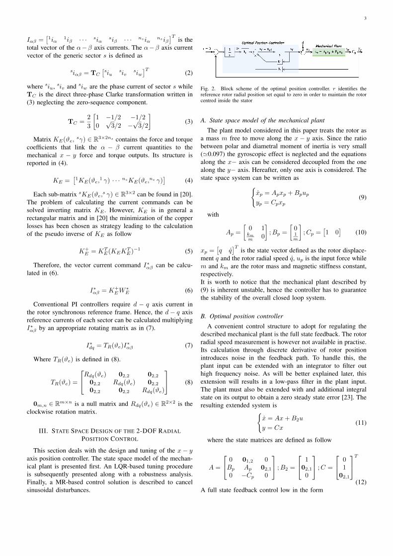
Fig. 3. Block scheme of the MR position controller integrated in the optimalposition controller.
With reference to Fig. 2, L(s) is the open loop transferfunction from d to up. Ms is directly related to gain and phasemargin. Indeed, the quantity Ms is the inverse of the shortestdistance from the Nyquist curve of the open loop transferfunction to the critical point -1. For instance, a sensitivityMs < ξ0 guarantees that the distance from the critical pointto the Nyquist curve is always greater than 1/ξ0 and that theNyquist curve of the loop transfer function is always outsidea circle of radius 1
Msaround the critical point -1, known as
the sensitivity circle. Limiting Ms to values typically smallerthan ξ0 = 2 ensures good robustness of the closed loop system[26].Defining matrices C1, D11 and B1 in (15) as
C1 =[1 0 0 0
];D11 = 1;B1 =
[0 BTp 0
]T(18)
the closed loop transfer function from d to z∞ is equalto S(s) defined in (17). It is now possible to set an upperbound to Ms during the optimal controller syntheses in orderto increase the overall system robustness.
D. Integration of MRC in the optimal position control
In order to compensate the position oscillation, the relevantsystem state portion can be filtered by means of a dynamicsystem presenting high gain at the frequencies to be damped.A multi-frequency force disturbance causes a multi-frequencyposition oscillation, hence a set of dynamic systems, each ofthem designed to have high gain at a specific frequency, isrequired in this work. For this reason a set of filters is used,forming a MRC [15]. The inclusion of resonant controllerscomplicates, in general, the tuning of the resulting overallregulator. The presence of complex conjugate poles risk todestabilize the system as soon as the gains increase. In thiswork, the resonant controller are modelled in state spacedomain and have been included in the extended plant. In thisway it is possible to adopt the LQR tuning procedure describedin previous subsection solving the tuning problem.The state space equation of the nth filter is{
xr,n = Ar,nxr,n +Br,nur
yr,n = Cr,nxr,n(19)
where xr,n is the state vector and Ar,n, Br,n, Cr,n are definedas
Ar,n =
[0 1−ω2
n 0
];Br,n =
[0ω2n
];Cr,n =
[1 0
](20)
5
with ωn = 2πfn the resonant pulsation.In the proposed paper the first 4 harmonics of the rotatingpulsation are compensated. Hence, defining ωm the rotatingspeed in [rad/s], the n = 4 resonant pulsations are: ω1 = ωm,ω2 = 2ω1, ω3 = 3ω1 and ω4 = 4ω1. Equation (21) shows thestate space formulation of the MRC.{
xr = Arxr +Brur
yr = Crxr(21)
where Ar and Cr are block diagonal matrices defined asdiag(Ar,1, · · · , Ar,n) and diag(Cr,1, · · · , Cr,n) respectivelywhile the macro-vector Br is defined piling the vectors Br,n.The output yr can now be inserted in the cost function (14)obtaining
JLQR =
∫ ∞0
[xTQx+ yTr Qryr + uTRu]dt =∫ ∞0
[xTQx+ xTr CTr QrCrxr + uTRu]dt (22)
where Qr is the state weight matrix of the MRC that willbe defined in the next section. Defining the augmented statex =
[x xr
]T, (22) becomes
JLQR =
∫ ∞0
[xT Qx+ uTRu]dt (23)
where Q =
[Q 04,8
08,4 CTr QrCr
]. (23) is the conventional
LQR cost function for the augmented system
˙x = Ax+ B2u (24)
A and B2 are defined as follow
A =
[A 04,8
Wr Ar
];Wr = −BrC; B2 =
[B2
08,1
](25)
System (24) is obtained merging systems (15) and (21)and assuming the rotor position as input of the MRC (21).Minimizing the cost function (23) results in a state feedbackcontrol law in the form
u = −Kx = −[Ke −Kr
] [ xxr
](26)
The resulting control structure is depicted in Fig. 3. Thepresented controller has been designed to compensate 4 spe-cific frequencies, however it is straightforward to customize(21) for any order n.
The synthesis of the optimal controller can be carried outfollowing the formulation presented in the previous subsectiononce matrices A and B2 are replaced with A and B2 in (15).Furthermore, C1, B1, C2 and D22 have to be re-written takinginto account the considered MRC as follow
C1 =[C1 01,8
]; B1 =
[B1
08,1
]; C2 =
[√Q
01,12
]; D22 =
[012,1√R
](27)
while D11 remains unchanged.
Real axis [rad/s]
-1500 -1000 -500 0 500
Imagin
ary
axis
[ra
d/s
]
-2000
-1000
0
1000
2000a) MRC tuned for a single speed value
2π10 [rad/s]
2π20 [rad/s]
2π30 [rad/s]
2π40 [rad/s]
2π50 [rad/s]-4 0 4
-500
0
500
Zoom
-1000 -500 0 500
Real axis [rad/s]
-2000
-1000
0
1000
2000
Imagin
ary
axis
[ra
d/s
]
b) MRC tuned for different speed values2π10 [rad/s]
2π20 [rad/s]
2π30 [rad/s]
2π40 [rad/s]
2π50 [rad/s]-80 -60 -40 -20 0
-2000
0
2000
Zoom
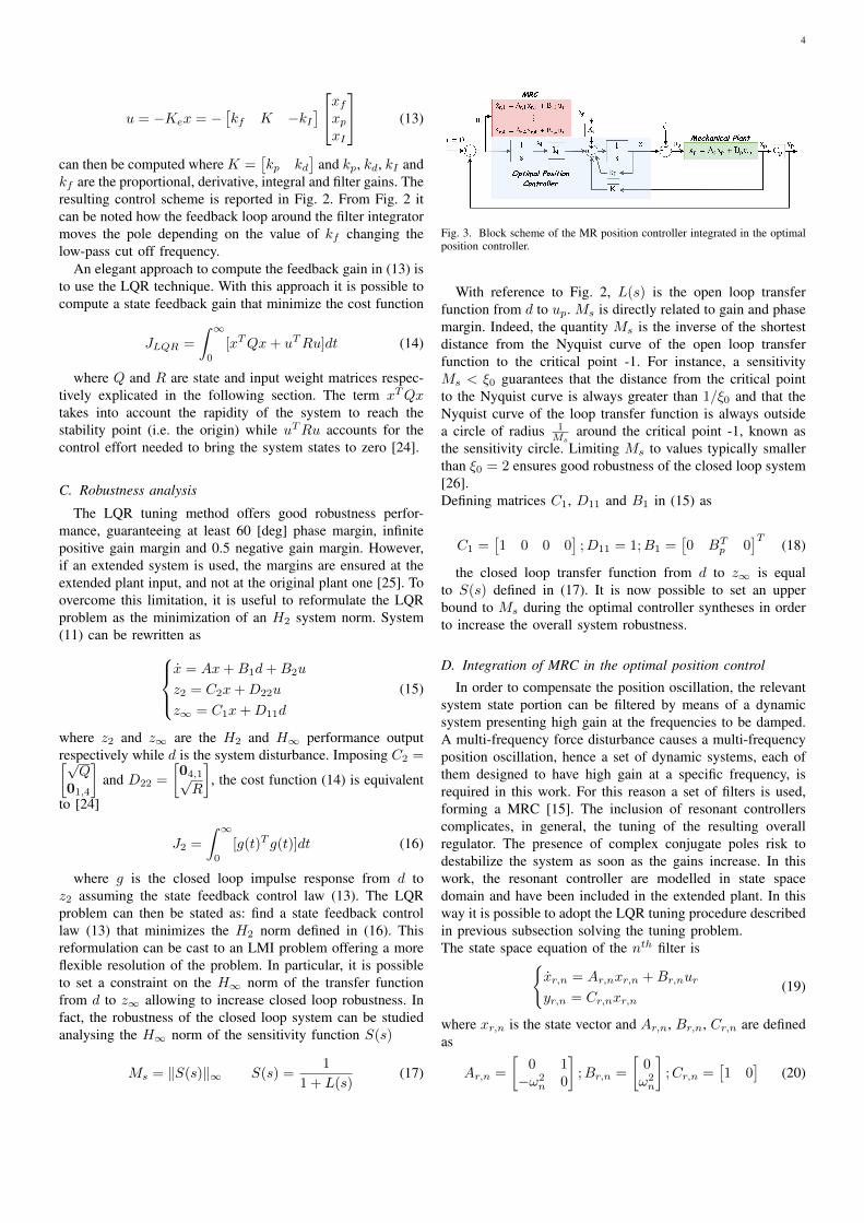
Fig. 4. Poles map of the MRC controller: a) tuning with a single speed value;b) tuning with different speed values to cover the operative speed range.
1 2 3 4 5 6 7 8 9 100
1
2
3
Magn
itu
de
[ab
s]
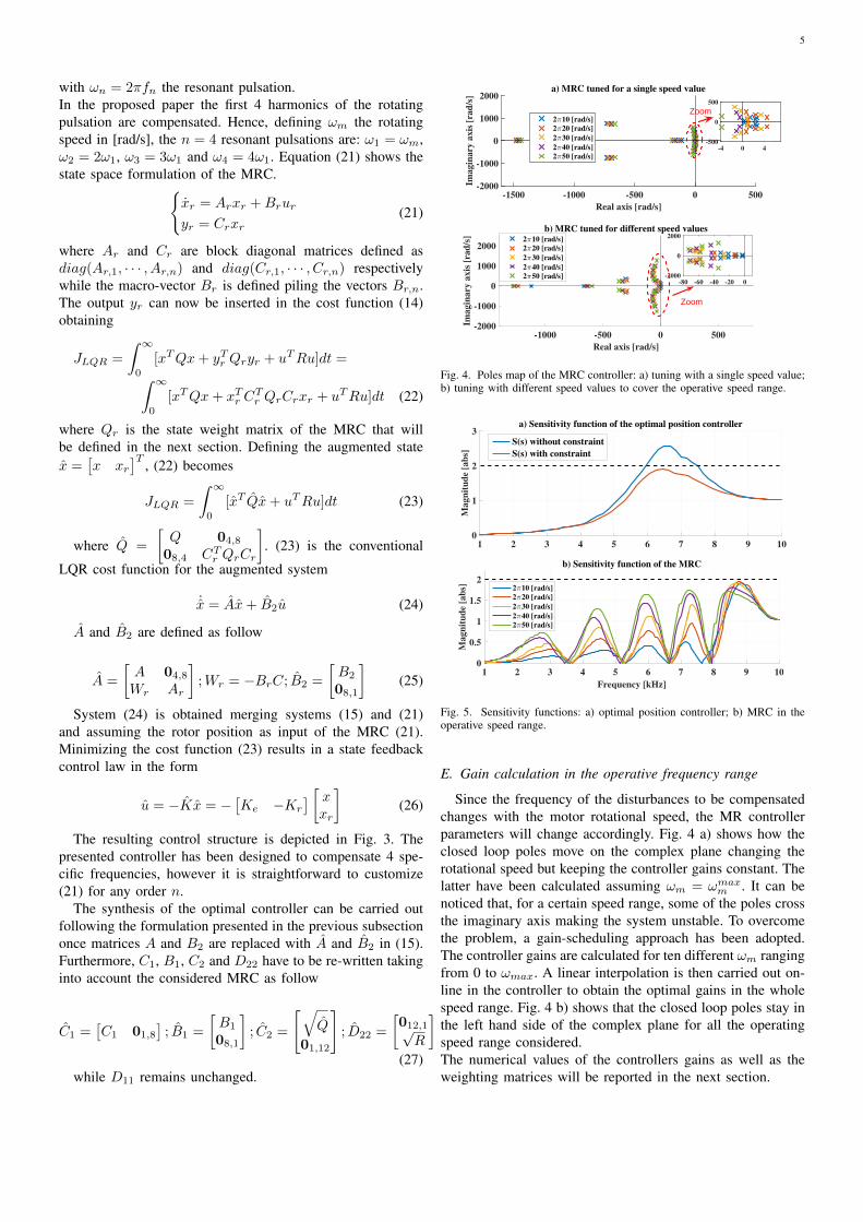
a) Sensitivity function of the optimal position controller
S(s) without constraint
S(s) with constraint
1 2 3 4 5 6 7 8 9 10
Frequency [kHz]
0
0.5
1
1.5
2
Magn
itu
de
[ab
s]
b) Sensitivity function of the MRC
2π10 [rad/s]
2π20 [rad/s]
2π30 [rad/s]
2π40 [rad/s]
2π50 [rad/s]
Fig. 5. Sensitivity functions: a) optimal position controller; b) MRC in theoperative speed range.
E. Gain calculation in the operative frequency range
Since the frequency of the disturbances to be compensatedchanges with the motor rotational speed, the MR controllerparameters will change accordingly. Fig. 4 a) shows how theclosed loop poles move on the complex plane changing therotational speed but keeping the controller gains constant. Thelatter have been calculated assuming ωm = ωmaxm . It can benoticed that, for a certain speed range, some of the poles crossthe imaginary axis making the system unstable. To overcomethe problem, a gain-scheduling approach has been adopted.The controller gains are calculated for ten different ωm rangingfrom 0 to ωmax. A linear interpolation is then carried out on-line in the controller to obtain the optimal gains in the wholespeed range. Fig. 4 b) shows that the closed loop poles stay inthe left hand side of the complex plane for all the operatingspeed range considered.The numerical values of the controllers gains as well as theweighting matrices will be reported in the next section.
6
TABLE IISTANDARD CONTROLLER GAINS
Parameter gain Valuekf (×103) 2.3303kp (×109) 4.4816kd (×106) 7.6553kI (×1011) 5.4753
IV. SIMULATION RESULTS
A. Numerical values of the controllers gains
The feedback vector Ke of the standard controller canbe obtained setting the weighting matrices Q and R. Theirchoice is the key problem in the design of optimal controllerswith the LQR method and it is often based on the designerexperience. Indeed, iterative and trial and error approaches areconventionally used to determine those values of Q and R thatprovide the desired system response. The same has been donefor the considered position controller. In particular, both sidesof (14) have been divided by R, defined as a scalar quantityfor this controller. The operation scales the cost function JLQRbut does not change its shape. Therefore, only the weights ofmatrix Q have to be defined. Increasing the integral weightproduces a fast reference signal response while increasing thestates weights produces the opposite effect, hence Q has beenset equal to diag(0, 0, 0, qI). On the other hand, high valuesof qI result in high low pass filter cut-off frequencies, henceworst noise rejection capabilities. Therefore, the choice of qIis a trade off between a good system dynamic and a good noiserejection. The integral weight qI was chosen equal to 3e23 inthis work. Furthermore, the sensitivity function is constrainedsetting the value of ξ0 equal to 2. The controller gains obtainedare reported in Table II. Fig. 5 reports a comparison betweenthe sensitivity function of the LQR controller described inSection III-B and the robust one described in Section III-C.As can be noted, in the second case, the sensitivity functiondoes not exceed the setting value ξ0 enhancing the systemrobustness.In the MRC considered in this work n = 4 hence the size ofthe feedback vector K is 12, where the first four elementscorrespond to Ke while the remaining eight ones are theresonant state vector gains. R and ξ0 remain unchanged whileQ has to be used as weighting matrix including Q, previouslydefined, and Qr = diag(10qr, 8qr, 6qr, 4qr) where qr is setequal to 1e17. Table III shows the gain values for the tenoperating speeds considered, covering the operative frequencyrange. Furthermore, Fig.5 b) shows that the sensitivity functionis maintained below ξ0 for the all speed range.
B. Simulation model
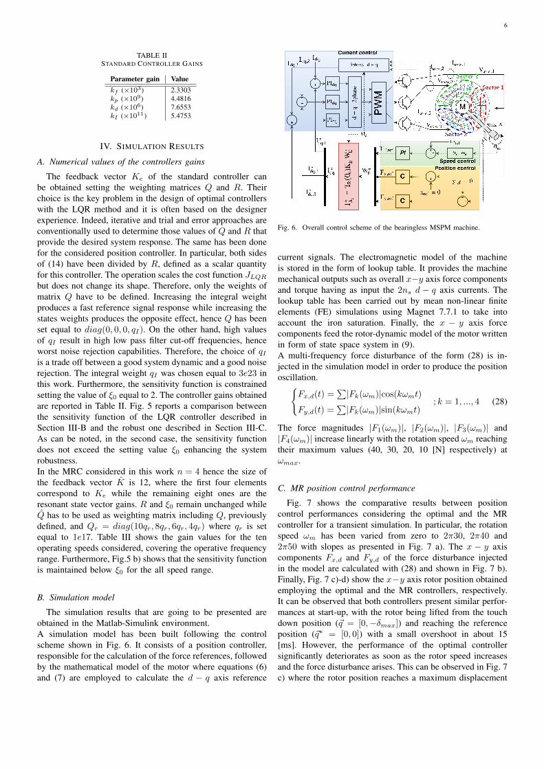
The simulation results that are going to be presented areobtained in the Matlab-Simulink environment.A simulation model has been built following the controlscheme shown in Fig. 6. It consists of a position controller,responsible for the calculation of the force references, followedby the mathematical model of the motor where equations (6)and (7) are employed to calculate the d − q axis reference
Fig. 6. Overall control scheme of the bearingless MSPM machine.
current signals. The electromagnetic model of the machineis stored in the form of lookup table. It provides the machinemechanical outputs such as overall x−y axis force componentsand torque having as input the 2ns d − q axis currents. Thelookup table has been carried out by mean non-linear finiteelements (FE) simulations using Magnet 7.7.1 to take intoaccount the iron saturation. Finally, the x − y axis forcecomponents feed the rotor-dynamic model of the motor writtenin form of state space system in (9).A multi-frequency force disturbance of the form (28) is in-jected in the simulation model in order to produce the positionoscillation.{
Fx,d(t) =∑|Fk(ωm)|cos(kωmt)
Fy,d(t) =∑|Fk(ωm)|sin(kωmt)
; k = 1, ..., 4 (28)
The force magnitudes |F1(ωm)|, |F2(ωm)|, |F3(ωm)| and|F4(ωm)| increase linearly with the rotation speed ωm reachingtheir maximum values (40, 30, 20, 10 [N] respectively) atωmax.
C. MR position control performance
Fig. 7 shows the comparative results between positioncontrol performances considering the optimal and the MRcontroller for a transient simulation. In particular, the rotationspeed ωm has been varied from zero to 2π30, 2π40 and2π50 with slopes as presented in Fig. 7 a). The x − y axiscomponents Fx,d and Fy,d of the force disturbance injectedin the model are calculated with (28) and shown in Fig. 7 b).Finally, Fig. 7 c)-d) show the x−y axis rotor position obtainedemploying the optimal and the MR controllers, respectively.It can be observed that both controllers present similar perfor-mances at start-up, with the rotor being lifted from the touchdown position (~q = [0,−δmax]) and reaching the referenceposition (~q∗ = [0, 0]) with a small overshoot in about 15[ms]. However, the performance of the optimal controllersignificantly deteriorates as soon as the rotor speed increasesand the force disturbance arises. This can be observed in Fig. 7c) where the rotor position reaches a maximum displacement

7
TABLE IIIMR CONTROLLER GAINS
Parameter gain 2π5 2π10 2π15 2π20 2π25 2π30 2π35 2π40 2π45 2π50
kf (×103) 2.3898 2.5325 2.6862 2.8112 2.8983 2.9579 2.9935 3.0159 3.0245 3.0309kp (×109) 4.8086 5.6651 6.7092 7.6302 8.3088 8.7607 9.0051 9.1077 9.0863 9.0089kd (×107) 0.8034 0.9011 1.0163 1.1155 1.1901 1.2433 1.2778 1.2993 1.3100 1.3141kI (×1011) 5.4742 5.4691 5.4771 5.4702 5.4726 5.4742 5.4709 5.4708 5.4653 5.46401kr,1 (×108) 8.6636 7.9634 6.3956 4.5581 2.8278 1.2083 -0.2847 -1.6428 -2.8747 -4.00152kr,1 (×106) 8.8506 8.8598 7.9997 6.9851 6.0445 5.2336 4.5215 3.9108 3.3706 2.89681kr,2 (×108) 7.5443 4.7120 1.4754 -1.3529 -3.5946 -5.3388 -6.6589 -7.6370 -8.3008 -8.70792kr,2 (×106) 7.1009 5.9927 4.6647 3.5085 2.5955 1.8954 1.3467 0.9128 0.5632 0.28231kr,3 (×108) 6.4065 3.3975 -0.0301 -2.9718 -5.1356 -6.5840 -7.3986 -7.7001 -7.5736 -7.15252kr,3 (×106) 4.4869 3.6767 2.7350 1.8940 1.2241 0.7149 0.3308 0.0470 -0.1581 -0.30061kr,4 (×108) 5.8283 4.0060 0.8680 -2.3267 -4.6635 -5.9415 -6.2956 -6.0075 -5.3120 -4.43382kr,4 (×106) 1.8761 1.9429 1.6609 1.1691 0.6764 0.2814 -0.0016 -0.1860 -0.2964 -0.3539
0 0.1 0.2 0.3 0.4 0.5 0.6 0.7 0.8 0.9 10
10
20
30
40
50
Sp
eed
[H
z]
a) Rotating speed
0 0.2 0.4 0.6 0.8 1-100
-50
0
50
100
Forc
e d
istu
rbe
[N]
b) Force disturbe
x-axis force
y-axis force
0 0.2 0.4 0.6 0.8 1-150
-100
-50
0
50
100
Posi
tion
[µ
m]
c) Radial position for optimal control
x-axis position
y-axis position
0 0.01 0.02-150-100
-500
0 0.2 0.4 0.6 0.8 1
Time [s]
-150
-100
-50
0
50
Posi
tion
[µ
m]
d) Radial position for MR control
x-axis position
y-axis position
0 0.01 0.02-150-100
-500
Fig. 7. Simulative comparison between optimal and MR position controllersduring a speed transient: a) rotating speed; b) force disturbance; c) x − yaxis position with optimal position controller; d) x−y axis position with MRposition controller.
of around 90 [µm] when the rotation speed is 2π50 [rad/s]and the force disturbance presents its maximum magnitudeand frequency. Therefore, a MRC is required to guaranteea good performance in the bearingless operation. Fig. 7 d)shows that the MRC introduced effectively suppresses themulti-frequency oscillation after a short transient in the wholeoperating speed range.The following section will present the experimental results ob-tained with both position controllers on a prototype bearinglessMSPM machine.
Fig. 8. Experimental rig: a) the three three-phase inverters; b) the controlboard; c) the machine prototype and test rig; d) the rotor shaft with thedisplacement sensors.
V. EXPERIMENTAL RESULTS
A. Description of the experimental set-up
The experimental set-up is detailed in all its parts in Fig. 8.Fig. 8 a) shows the three three-phase inverters, each of themconnected to one of the MSPM motor winding (Fig. 8 c)).The power module of the single inverter is a dual-in-linepackage intelligent power module (PS21A79) manufacturedby Mitsubishi Semiconductor operated at 10 [kHz] switchingfrequency. The industrial control boards mounted on eachinverter have been removed and substituted by one centralizedand custom made control platform [27] (Fig. 8 b)) thatcommunicates with the power modules gate drives by meansof fibre optics cables.In the presented bearingless drive two degrees of freedom areactively controlled, hence the tilting movement and the axialdisplacement must be constrained by a self-alignment bearingmounted on one side of the shaft. The other side is free tomove along the x−y axes within a certain displacement givenby the clearance δmax of the backup bearing. Fig. 8 d) showsthe two eddy currents displacement probes mounted on thebackup bearing housing along the x− y axes.

8
-150 -100 -50 0 50 100 150-150
-100
-50
0
50
100
150
Y-p
osi
tio
n [µ
m]
a) 30 [Hz] rotating speed
-150 -100 -50 0 50 100 150
X-position [µ m]
b) 40 [Hz] rotating speed
Backup bearing inner surface
Rotor position for optimal position controller
Rotor position for MR position controller
-150 -100 -50 0 50 100 150
c) 50 [Hz] rotating speed
Fig. 9. Rotor trajectory obtained with the optimal and with the MR position controllers: a) 30 [Hz] rotating speed; b) 40 [Hz] rotating speed; c) 50 [Hz]rotating speed.
0
5
10
0
5
10
0
5
10
Posi
tion
[µ
m]
0
5
10
0 100 200 300 400 500
Frequency [Hz]
0
5
10
0 100 200 300 400 500
Frequency [Hz]
0
5
10
MR controllerOptimal controller
30 [Hz] 30 [Hz]
40 [Hz] 40 [Hz]
50 [Hz] 50 [Hz]
Fig. 10. Harmonic spectrum carried out with the fast Fourier transform ofthe x−axis position measurement. The compensation of the multi-frequencyposition oscillation can be appreciated.
B. Periodic disturbance suppression
The suppression of the multi-frequency position oscilla-tion has been tested for three different operating speeds(ωm = 2π30, 2π40, 2π50 [rad/s]) in order to experimentallyvalidate the stability of the position controllers in the operativespeed range. Fig. 9 a)-c) shows the rotor trajectory in ax − y plane. It can be noticed that both the optimal andthe MR position controllers can achieve a more performingbearingless operation keeping the rotor element well far fromthe backup bearing inner surface. From the figures it canalso be observed that the MRC significantly improves thelevitation performances maintaining the rotor displacementwithin 10 [µm] against the 40 [µm] of the optimal controller.The harmonic spectrum of the x−axis position for the threerotation speeds considered is presented in Fig. 10. It can bewell appreciated how the MRC manages to damp the first fourposition harmonics corresponding to the pulsations ω1 = ωm,ω2 = 2ω1, ω3 = 3ω1 and ω4 = 4ω1.The previous experimental results validate the improvementsin terms of levitation performances of the MRC respect tothe optimal one in steady state operating conditions. However,the rapidity of damping the position oscillation should also betaken into account in the analysis, hence a transient test hasbeen performed running the motor progressively from standstill to 2π30, 2π40 and 2π50 [Hz] within one second. The
0 0.2 0.4 0.6 0.8 1-20
0
20
40
60
Sp
eed
[H
z]
a) Rotating speed
Measured speed
Speed reference
0 0.2 0.4 0.6 0.8 1
Time [s]
-50
0
50
100
150
Posi
tion
[µ
m]
b) x-y axis postion
x-y axis postion reference
x-axis position
y-axis position
0 0.01 0.02
0
50
100
Fig. 11. Transient test results using the MRC: a) rotating speed; b) x − yaxis position measurement.
results are presented in Fig. 11 a) and b). The MR positioncontroller is activated after 10 [ms] and the rotor reaches thereference position in about 15 [ms] (Fig. 11 b)), which isin good agreement with the simulation result obtained. Thenthe rotor is accelerated as shown in Fig. 11 a) and the MRCquickly operates to damp the position oscillation during thespeed variations (Fig. 11 b)).
VI. CONCLUSIONS
In the presented work the theoretical principles of the torqueand suspension force generation of the bearingless MSPMmachine have been illustrated. The obtained mathematicalmodel has been exploited to calculate the optimal referencecurrent signals targeting the minimization of the Joule losses.Then, a robust optimal position controller is introduced andsynthesized following a state space approach. The LQRand the LMI techniques have been adopted to calculate thecontrollers gains taking into account the robustness of theoverall closed loop system. A multi-resonant controller hasbeen finally added to compensate the periodic disturbances. Acomparison of the two proposed controllers is carried out by

9
means of numerical simulations aiming the compensation ofthe periodic disturbance.Finally, the proposed position controller design is validatedexperimentally on a prototype bearingless MSPM machineshowing that the MRC performs an effective rejection of theposition oscillations enhancing the levitation performance ofthe bearingless drive.
REFERENCES
[1] P. Hermann, “A radial active magnetic bearing,” London Patent, no. 1,p. 478, 1973.
[2] X. Sun, L. Chen, and Z. Yang, “Overview of bearingless permanent-magnet synchronous motors,” IEEE Transactions on Industrial Elec-tronics, vol. 60, no. 12, pp. 5528–5538, Dec 2013.
[3] T. Baumgartner, R. M. Burkart, and J. W. Kolar, “Analysis and design ofa 300-w 500000-r/min slotless self-bearing permanent-magnet motor,”IEEE Transactions on Industrial Electronics, vol. 61, no. 8, pp. 4326–4336, Aug 2014.
[4] A. H. Pesch, A. Smirnov, O. Pyrhnen, and J. T. Sawicki, “Magneticbearing spindle tool tracking through µ -synthesis robust control,”IEEE/ASME Transactions on Mechatronics, vol. 20, no. 3, pp. 1448–1457, June 2015.
[5] S. Y. Zhang, C. B. Wei, J. Li, and J. H. Wu, “Robust h infinity controllerbased on multi-objective genetic algorithms for active magnetic bearingapplied to cryogenic centrifugal compressor,” in 2017 29th ChineseControl And Decision Conference (CCDC), May 2017, pp. 46–51.
[6] A. Chiba, T. Fukao, O. Ichikawa, M. Oshima, M. Takemoto, and D. G.Dorrell, Magnetic bearings and bearingless drives. Elsevier, 2005.
[7] J. Asama, T. Fukao, A. Chiba, A. Rahman, and T. Oiwa, “A designconsideration of a novel bearingless disk motor for artificial hearts,” in2009 IEEE Energy Conversion Congress and Exposition, Sept 2009, pp.1693–1699.
[8] K. Inagaki, A. Chiba, M. A. Rahman, and T. Fukao, “Performancecharacteristics of inset-type permanent magnet bearingless motor drives,”in 2000 IEEE Power Engineering Society Winter Meeting. ConferenceProceedings (Cat. No.00CH37077), vol. 1, 2000, pp. 202–207 vol.1.
[9] J. Huang, B. Li, H. Jiang, and M. Kang, “Analysis and control of mul-tiphase permanent-magnet bearingless motor with a single set of half-coiled winding,” IEEE Transactions on Industrial Electronics, vol. 61,no. 7, pp. 3137–3145, July 2014.
[10] S. Kobayashi, M. Ooshima, and M. N. Uddin, “A radial position controlmethod of bearingless motor based on d - q -axis current control,” IEEETrans. on Ind. Appl., vol. 49, no. 4, pp. 1827–1835, July 2013.
[11] G. Valente, L. Papini, A. Formentini, C. Gerada, and P. Zanchetta,“Radial force control of multi-sector permanent magnet machines forvibration suppression,” IEEE Transactions on Industrial Electronics,vol. PP, no. 99, pp. 1–1, 2017.
[12] G. Sala, G. Valente, A. Formentini, L. Papini, D. Gerada, P. Zanchetta,A. Tani, and C. Gerada, “Space vectors and pseudo inverse matrix meth-ods for the radial force control in bearingless multi-sector permanentmagnet machines,” IEEE Transactions on Industrial Electronics, vol. PP,no. 99, pp. 1–1, 2018.
[13] R. Herzog, P. Buhler, C. Gahler, and R. Larsonneur, “Unbalance com-pensation using generalized notch filters in the multivariable feedback ofmagnetic bearings,” IEEE Transactions on Control Systems Technology,vol. 4, no. 5, pp. 580–586, Sep 1996.
[14] C. Peng, J. Fang, and X. Xu, “Mismatched disturbance rejectioncontrol for voltage-controlled active magnetic bearing via state-spacedisturbance observer,” IEEE Transactions on Power Electronics, vol. 30,no. 5, pp. 2753–2762, May 2015.
[15] C. Peng, J. Sun, X. Song, and J. Fang, “Frequency-varying currentharmonics for active magnetic bearing via multiple resonant controllers,”IEEE Transactions on Industrial Electronics, vol. 64, no. 1, pp. 517–526,Jan 2017.
[16] A. Laiho, A. Sinervo, J. Orivuori, K. Tammi, A. Arkkio, and K. Zenger,“Attenuation of harmonic rotor vibration in a cage rotor induction ma-chine by a self-bearing force actuator,” IEEE Transactions on Magnetics,vol. 45, no. 12, pp. 5388–5398, Dec 2009.
[17] A. Sinervo and A. Arkkio, “Rotor radial position control and its effect onthe total efficiency of a bearingless induction motor with a cage rotor,”IEEE Transactions on Magnetics, vol. 50, no. 4, pp. 1–9, April 2014.
[18] A. Sinervo, A. Laiho, and A. Arkkio, “Low-frequency oscillation inrotor vibration of a two-pole induction machine with extra four-polestator winding,” IEEE Transactions on Magnetics, vol. 47, no. 9, pp.2292–2302, Sept 2011.
[19] A. Chiba, T. Fukao, and M. A. Rahman, “Vibration suppression of aflexible shaft with a simplified bearingless induction motor drive,” IEEETrans. on Industry Applic., vol. 44, no. 3, pp. 745–752, May 2008.
[20] G. Valente, L. Papini, A. Formentini, C. Gerada, and P. Zanchetta,“Radial force control of multi-sector permanent magnet machines,” in2016 XXII Inter. Conf. on Electrical Machines (ICEM), Sept 2016, pp.2595–2601.
[21] G.Valente, L. Papini, A. Formentini, C. Gerada, and P. Zanchetta, “Ra-dial force control of multi-sector permanent magnet machines consid-ering radial rotor displacement,” in 2017 IEEE Workshop on ElectricalMachines Design, Control and Diagnosis (WEMDCD), April 2017, pp.140–145.
[22] P. Bolognesi, “A mid-complexity analysis of long-drum-type electricmachines suitable for circuital modeling,” in 2008 18th InternationalConference on Electrical Machines, Sept 2008, pp. 1–5.
[23] G. F. Franklin, J. D. Powell, A. Emami-Naeini, and J. D. Powell,Feedback control of dynamic systems. Addison-Wesley Reading, MA,1994, vol. 3.
[24] J. B. Burl, Linear optimal control: H (2) and H (Infinity) methods.Addison-Wesley Longman Publishing Co., Inc., 1998.
[25] B. D. Anderson and J. B. Moore, Optimal control: linear quadraticmethods. Courier Corporation, 2007.
[26] S. Skogestad and I. Postlethwaite, Multivariable feedback control:analysis and design. Wiley New York, 2007, vol. 2.
[27] A. Galassini, G. L. Calzo, A. Formentini, C. Gerada, P. Zanchetta, andA. Costabeber, “ucube: Control platform for power electronics,” in 2017IEEE Workshop on Electrical Machines Design, Control and Diagnosis(WEMDCD), April 2017, pp. 216–221.
G. Valente received his Bachelor degree in EnergyEngineering in 2011 and his Master degree inElectrical Engineering in 2014 both from theUniversity of Padova, Italy. Between 2013 and2014 he developed sensorless control techniquesfor PMSM for his Master thesis at the Universityof Oviedo, Spain. He is now working towards itsPh.D. with the Power Electronics, Machines andControl Group, University of Nottingham, UK.His main research interest is design and control ofelectrical machines.
A. Formentini was born in Genova, Italy,in 1985. He received the M.S. degree incomputer engineering and the PhD degree inelectrical engineering from the University ofGenova, Genova, in 2010 and 2014 respectively.He is currently working as research fellowin the Power Electronics, Machines andControl Group, University of Nottingham.His research interests include control systemsapplied to electrical machine drives and powerconverters.
L. Papini received his Bachelor degree (Hons.)and Master degree (Hons.) in Electrical engineeringin 2009 and 2011, respectively, both from theUniversity of Pisa, Italy. He’s been a visitingstudent at The University of Nottingham, UK,developing analytical and numerical models forelectrical machines. From June to November 2011he collaborated with the Department of EnergyEngineering, University of Pisa, as a researchassistant. He is currently working towards its Ph.D.with the Power Electronic, Motors and Drives
Group at University of Nottingham. Since 2013 hold a position of researchassistant in the same institution. His main research interests are high speed,high power density electric machines, machine control and levitating system.

10
C. Gerada (M 05) received the Ph.D. degree innumerical modeling of electrical machines from theUniversity of Nottingham, Nottingham, U.K., in2005. He subsequently worked as a Researcher atthe University of Nottingham on high-performanceelectrical drives and on the design and modeling ofelectromagnetic actuators for aerospace applications.He was appointed as Lecturer in electrical machinesin 2008, Associate Professor in 2011, and Professorin 2013. His core research interests include thedesign and modeling of high-performance electric
drives and machines. Prof. Gerada is an Associate Editor of the IEEETransaction on Industry Applications.
P. Zanchetta (M 00, SM 15) received his MEngdegree in Electronic Engineering and his Ph.D. inElectrical Engineering from the Technical Universityof Bari (Italy) in 1993 and 1997 respectively. In 1998he became Assistant Professor of Power Electronicsat the same University. In 2001 he became lecturerin control of power electronics systems in the PEMCresearch group at the University of Nottingham UK,where he is now Professor in Control of PowerElectronics systems. He has published over 270 peerreviewed papers and he is Senior Member of the
IEEE. He is Chair of the IAS Industrial Power Converter Committee IPCCand member of the European Power Electronics (EPE) executive board. Hisresearch interests include control of power converters and drives, Matrix andmultilevel converters, power electronics for energy and transportation.