performance indices of soft computing models to …
TRANSCRIPT

Journal of Thermal Engineering, Vol. 3, No. 4, Special Issue 5, pp. 1358-1374, August, 2017 Yildiz Technical University Press, Istanbul, Turkey
This paper was recommended for publication in revised form by Regional Editor Omid Mahian 1 Energy Engineering Program, Izmir Institute of Technology, Izmir, Turkey
2 Department of Architecture, Izmir Institute of Technology, Izmir, Turkey
*E-mail: [email protected] Manuscript Received 21 June 2016, Accepted 20 September 2016
PERFORMANCE INDICES OF SOFT COMPUTING MODELS TO PREDICT THE
HEAT LOAD OF BUILDINGS IN TERMS OF ARCHITECTURAL INDICATORS
C.Turhan1, T. Kazanasmaz
2, G. Gökçen Akkurt
1*
ABSTRACT
This study estimates the heat load of buildings in Izmir/Turkey by three soft computing (SC) methods; Artificial
Neural Networks (ANNs), Fuzzy Logic (FL) and Adaptive Neuro-based Fuzzy Inference System (ANFIS) and
compares their prediction indices. Obtaining knowledge about what the heat load of buildings would be in
architectural design stage is necessary to forecast the building performance and take precautions against any
possible failure. The best accuracy and prediction power of novel soft computing techniques would assist the
practical way of this process. For this purpose, four inputs, namely, wall overall heat transfer coefficient,
building area/ volume ratio, total external surface area and total window area/total external surface area ratio
were employed in each model of this study. The predicted heat load is evaluated comparatively using simulation
outputs. The ANN model estimated the heat load of the case apartments with a rate of 97.7% and the MAPE of
5.06%; while these ratios are 98.6% and 3.56% in Mamdani fuzzy inference systems (FL); 99.0% and 2.43% in
ANFIS. When these values were compared, it was found that the ANFIS model has become the best learning
technique among the others and can be applicable in building energy performance studies.
Keywords: Heat Load, Residential Buildings, ANN, Fuzzy Logic, ANFIS, Soft Computing
INTRODUCTION AND REVIEW
A wide variety of modelling techniques provide possibilities to predict energy consumption and the heat
load of the buildings in recent years, such as simple regression techniques [1-3], dynamic simulation tools [4-6],
artificial neural networks (ANNs) [7-10], adaptive-network based fuzzy inference systems (ANFIS) [11,12], the
hybrid optimization algorithm [13,14] and fuzzy logic (FL) approaches [15-18]. The significance is based on
their applicability and accuracy; that is their ability on how they achieve the outputs and in what kind of
precision they would correspond to the reality. Regression models predict well with more homogeneous data sets
but it is difficult or impossible to produce useful results for real-world problems. The performances of these
algorithms are not powerful when the problem becomes complex. Dynamic simulation tools are based on
physical methods which require certain guidelines and over-detailed modelling. Besides, these simulation tools
are expensive and complicated, making it difficult to use. Therefore, soft modelling (SC) methods including
ANNs, FL and ANFIS have become the novel tools to overcome any deficiencies observed in any other
techniques by reducing one of the total error indices which are mean absolute percentage error (MAPE), mean
squared error (MSE) or mean squared deviation (MSD) and root mean square error (RMSE). These models also
use the statistical criteria such as correlation coefficient (R) and multiple correlation coefficient (R2) for
goodness of fit. The error indices are expected to close to zero whilst the R and R2 should be as close as to 1 for
the best performance [11, 16-18].
The building sector represents the second-largest energy consumer accounting for 37 % of the total final
energy consumption (18 % in residential buildings, 19 % in non-residential buildings) in terms of final energy
consumption in Turkey. However, this sector presents significant energy saving opportunities for the cost-
effective energy, estimated at almost 30-50 % of the current energy consumption [19]. Heating energy
consumption has the highest share in total energy consumption of buildings [20]. Consequently, the heat load is
the basic numerical quantity to evaluate the energy consumption of buildings [7, 21]. The estimation of heat load
is necessary, both for the new existing buildings which might be renovated to improve their energy consumption.
Foreseeing early inaccuracies regarding the heat load might be avoided by designing appropriate wall overall
heat transfer coefficient, building area to volume ratio, total external surface area and total window area to total
Journal of Thermal Engineering, Research Article Vol. 3, No. 4, Special Issue 5, pp. 1358-1374, August, 2017
1359
external surface area ratio. Thus, the heat load and energy consumption might be evaluated simply and rapidly in
the early design stage.
Considering the existing buildings, it might not be possible to obtain the architectural or mechanical
drawings where the above mentioned parameters can be taken. If this is the case, the parameters can be obtained
by field measurements. While renovating the existing buildings, the estimation of heat loads would guide
professionals about what type of precautions or what type of renovation strategies might be taken into
consideration.
To evaluate the heat load, ANNs are recently accepted alternative artificial intelligence methods offering
a way to tackle non-linear and complex problems. Turhan et al. [7] and Ekici and Aksoy [22] succeeded to
predict the heat load of existing buildings implementing a back propagation ANN model with a multiple
correlation coefficient of 0.9774 and 0.948-0.985 (comparing with building energy simulation model results),
respectively. Another study employed 8 input parameters (relative compactness, surface area, wall area, roof
area, overall height, orientation, glazing area and glazing distribution) in the ANN model to estimate the heating
and cooling load of buildings [23]. One issue which needs to be discussed is that ANNs are black box models
which make them more challenging to interpret. The model offers a weight matrix which is optimized after
thousands of iterations. Furthermore, limited or noisy training data result in an illogical and meaningless output.
Fuzzy logic (FL) is an evolving method which has the ability to describe the knowledge in a descriptive
human-like manner in the form of simple rules using linguistic variables [24]. The fuzzy system contains a set of
rules which were developed from qualitative descriptions which makes it user friendly. During last decades, a
few studies have published on predicting energy consumption of buildings. Chibattoni et al. [16] conducted a
fuzzy logic energy consumption model for Italian residential buildings using the occupancy activity and typical
domestic habits. The model was validated with electricity demand data recorded over the period of one year.
The mean error of the model was found as 0.52% which was acceptable as quite successful prediction. Kabak et
al. [17], implemented fuzzy multi-criteria decision making approach in order to analyse BEP-TR [25] energy
simulation tool. The study applied an approach to categorize alternative buildings according to their overall
energy performance. The criterion such as location and climate data, geometrical shape, building envelope,
mechanical systems, lighting system, hot water system and renewable energy and cogeneration was used for the
model. The impact of each criterion on energy consumption of buildings was analysed. Kajl et al. [26] created a
fuzzy logic model to correct the outputs by post-processing the results of neural networks. The fuzzy assistant
allows the user to determine the impact of eleven building parameters including length and width of buildings,
number of floors, R-value of exterior wall, fenestration and U-value of windows on the annual and monthly
energy consumption. The model was compared with DOE-2 [27] simulation tool results with a RMSE of 0.35.
Apart from these promising machine learning techniques, the combination of them is called ANFIS in
which the benefit of self-learning procedure of ANNs and simple structure of FL are apparent. The ANFIS model
was effective in forecasting the building energy consumption in cold regions, with a 0.965 prediction rate, when
transparency ratios, azimuth angles, building form factors and insulation thicknesses were used as the model
inputs [11]. Another study supported its performance and high accuracy similarly; however, the model had a time
consuming performance with different parameter configuration [28].
The question is whether gathering the strongest characterization of each technique (ANNs and FL) and
combining them in ANFIS would result in a higher prediction power or not? Goyal et al. (2014) compared
ANNs, FL and ANFIS and figured out that FL had the highest estimation rate, when the prediction of daily pan
evaporation was the case [29]. Applications and comparison of the SC methods are apparent in several research
areas apart from energy studies [30-33]. Islam [32] developed a number of AI techniques varying from ANNs to
FL to estimate electrical load in a company. The study showed that ANNs was principally attractive, as they were
capable of handling the nonlinear relationships between load and the factors affecting them directly from
historical data. Wang et al. [33] compared the performances of ANNs, autoregressive moving-average (ARMA),
ANFIS, support vector machine (SVR) and genetic programming (GP) models on forecasting monthly discharge
time series. The evaluation criteria contained the MAPE and the R. The ANFIS model was the best performed
technique with an R of 0.9322. A further study resulted in the highest estimation performance of neuro-fuzzy
systems to figure out the thermal diffusivity of building materials when compared to ANNs and inverse methods
[34].
This paper presents the comparison of three SC models, namely, ANNs, FL and ANFIS in the field of
predicting heat load of buildings. For the validation, the results are compared with a building simulation tool

Journal of Thermal Engineering, Research Article Vol. 3, No. 4, Special Issue 5, pp. 1358-1374, August, 2017
1360
which is called The Standard Assessment Procedure for Energy Rating of Dwellings software (KEP-IYTE-ESS)
[35]. The study also shows which SC method performs better on prediction of the heat load of buildings.
OVERVIEW OF SC TECHNIQUES
The SC methods which are used for the study are described in this section.
ANNs ANNs are data-driven mathematical models which resemble the biological nervous system [36]. Being
capable of capturing non-linear relationships among the parameters is ANNs’ superiority. The structure of the
ANNs is composed of parallel element units called neurons. A schematic representation of an ANN model is
shown in Figure 1.
Figure 1. Schematic representation of a feed forward ANN
ANNs have three layers-the input, hidden and output layers. Each layer is composed of a high number
of interconnected- and weighted- neurons transmitting the signals in the entire structure to produce the output.
Input layer is the incoming signals whilst output layer is the desired ones. Hidden layer is the connection
between input and output layers which stores the net information and transfer functions. The target output at each
output neuron is minimized by adjusting the weights and biases through some training algorithm. Scalar input
x1,x2 and x3 are multiplied by weight wnm and the weighted values are fed to the summing confluence. The
neuron has a bias bi that is summed with the weighted inputs in order to form the net input netj given in Eq. (1).
(netj) = x1 w1j + x2 w2j + …….+ xnwnj + bi (1)
The sigmoid function is usually employed as an activation function in the training step of the network.
The sigmoid function is expressed as Eq. (2):
y = 1/ (1+ e – netj) (2)
The objective of the model is to decrease error to an acceptable value that is called epoch or training
cycle. The error is expressed by the root-mean-squared error value (RMSE), which can be calculated with
following equation (3):
E=½[pΣiΣ|tip- oip|] ½ (3)
where (E) is the RMSE, t the network output, and o the desired output vectors over all the pattern (p).

Journal of Thermal Engineering, Research Article Vol. 3, No. 4, Special Issue 5, pp. 1358-1374, August, 2017
1361
FL Approach FL is a logical system which aims at a formulation of approximate reasoning. First, the approach was
proposed by Loutfi A. Zadeh in 1965 with the work “Fuzzy Theory” [37]. Zadeh defined the concept of Fuzzy
Sets as a class of objects with a continuum of grades of membership. Such a set is characterized by a
membership function which assigns to each object a grade of membership ranging between zero and one. After
1974, this technique was applied in many areas such as controlling of physical or chemical parameters like
temperature, electric current, flow of fluid and motion of machines [38]. The general structure of the FL
modelling is presented in Figure 2.
Figure 2. The structure of Fuzzy logic modelling
A fuzzy set is a generalization of an ordinary set by allowing a degree (or grade) of membership for
each element. Many degrees of membership are allowed in fuzzy sets. The degree of membership is indicated by
a number between 0 and 1. In extreme cases, if the degree is 0, the element does not belong to the set, and if 1,
the element belongs 100% to the set.
In a set, every element is associated with a degree of membership. This means that the membership function
(MF) of a set represents each element to its degree. The membership function assists the partial belongings
mathematically which have values between 0 and 1. It is formally written as Eq. 4.
µA (x): X → [0, 1] (4)
Basic relations for fuzzy sets are specified like in the ordinary sets. Fuzzy operations include union,
intersection, complement, binary relations and composition of relations as classical operations.
Fuzzy logic rules are called as contingent statements that describe the dependence of one or more linguistic
variable on another. The simple form of the basic lingual If-Then rule is shown as;
If “α” is A and “β” is B, then “λ” is C.
Here, the corresponding linguistic values are A, B and C while α, β and λ are the inputs. For example “if
temperature is HIGH the humidity is ZERO” is a fuzzy implication.
The model basically includes four components: fuzzification, fuzzy rule base, fuzzy output engine, and
fuzzification [38,39]. For each input and output variable selected is converted to degrees of membership by
fuzzification. It includes definition of fuzzy sets, determination of the degree of membership of crisp inputs in
appropriate fuzzy sets. All fuzzy variables are theoretically represented as a number between 0 and 1.In order to
obtain the fuzzy output, Fuzzy rule base form the basis for the fuzzy logic. It contains rules that cover all suitable
fuzzy relations between inputs and outputs. The fuzzy rule-based system uses IF-THEN rule based system given
by IF ascendant, THEN consequent [40]. Following rules are constituted for the example [41].
R1 : If x1 is LOW and x2 is SHORT then y is VILLAGE
R2 : If x1 is LOW and x2 is LONG then y is TOWN
R3 : If x1 is HIGH and x2 is SHORT then y is TOWN
R4 : If x1 is HIGH and x2 is LONG then y is TOWN
For the fourth rule; it is assumed as if the population of the settlement (x1) is high and the distance to the
furthest municipality (x2) is high then the rate of being municipality (y) is high.

Journal of Thermal Engineering, Research Article Vol. 3, No. 4, Special Issue 5, pp. 1358-1374, August, 2017
1362
Each fuzzy rule gives a single number that represents the truth value of that rule. All fuzzy rules are
taken into account by fuzzy inference engine in the fuzzy rule base. The fuzzy inference system is a framework
based on concepts of fuzzy set theorem, fuzzy if-then rules, and fuzzy reasoning. Conventional fuzzy inference
systems are typically built by domain experts and have been used in automatic control, decision analysis, and
expert systems. Optimization and adaptive techniques expand the applications of fuzzy inference systems to
fields such as adaptive control, adaptive signal processing, nonlinear regression, and pattern recognition. Fuzzy
inference system can take either fuzzy inputs or crisp inputs, but the outputs it produces are almost always fuzzy
sets. Sometimes it is necessary to have a crisp output, especially in a situation where a fuzzy inference system is
used as a controller. Therefore, a method of defuzzification is required to extract a crisp value that best represents
the fuzzy set. With crisp inputs and outputs, a fuzzy inference system implements a nonlinear mapping from its
input space to output space. This mapping is accomplished by a number of fuzzy if-then rules, each of which
describes the local behaviour of the mapping [42]. There are two methods widely used; the minimum and the
product operation methods. If “°” is the operator that indicates rule of inference, Eq. 5 can be written in terms of
membership function for minimum operator.
oB(y) = MAX [ MIN ( oA(x), oR(x,y) )] x ϵ E1 (5)
Similarly, Eq. 6 can be written in terms of membership function for prod operator.
oB(y) = MAX [ oA(x), oR(x,y)] x ϵ E1 (6)
Defuzzification converts fuzzy output set to crisp. It is necessary to convert the fuzzy quantities into
crisp quantities because generated fuzzy results cannot be used as such to the applications. Defuzzification can
also be called as “rounding off” method [39]. There are many defuzzification methods named as (COG)
(centroid), bisector of area (BOA), mean of maxima (MOM), leftmost maximum (LM), rightmost maximum
(RM), centre of sums and weighted average method [39]. Centroid method is the most widely used method as
expressed in Eq.7;
𝐾𝑥∗ =
∑ 𝜇(𝐾𝑖𝑥)𝐾𝑖𝑥𝑖
∑ 𝜇(𝐾𝑖𝑥)𝑖
(7)
𝐾𝑥∗ is the defuzzified output value,Kix is the output value in the ith subset, and μ(Kix) is the membership value of
the output value in the ith
subset.
ANFIS
ANFIS is the combination of ANNs and FL approaches which has adaptive nodes and directional links
[43]. With the ability of a fuzzy system and with the numeric power of a neural system adaptive network, ANFIS
has been shown to be powerful on prediction studies. Figure 3 shows the schematic representation of a typical
ANFIS model.

Journal of Thermal Engineering, Research Article Vol. 3, No. 4, Special Issue 5, pp. 1358-1374, August, 2017
1363
Figure 3. Architecture of ANFIS [43]
Figure 3 has two inputs (x and y) and one output (f). The model implements Sugeno-Takagi fuzzy
inference systems and if-then rules:
R1: IF x is A1 and y is B1 THEN f1= p1x + q1y+r1
R2: IF x is A2 and y is B2 THEN f2= p2x + q2y+r2
Here, Ai and Bi are the fuzzy sets, fi is the output and pi,qi and ri are the design parameters in training phases.
The nodes in ANFIS can be summarized as follows;
Layer 1: The layer that input variables are introduced to the system. The membership functions are used as node
functions.
Layer 2: The layer that the rules are constructed with the strength of corresponding layer.This layer generates
output.
Layer 3: The layer is an average layer that optimizes firing strength.
Layer 4: Consequent nodes that act as a defuzzifier.
Layer 5: Output nodes. The layer generates an output from the sum of each rule.
ANFIS uses training algorithm to optimize the design parameters to predict the desired output. When
the optimum parameters are found, the gradient descent method starts to adjust parameters corresponding to the
fuzzy sets in the input layer. Similarly, the output is calculated by applying the forward pass.
MODELLING THE HEAT LOAD OF BUILDINGS USING SC METHODS
Gathering the data
The subject matter is the residential building stock in İzmir (38.25 N, 27.08 E), Turkey, while the study
material itself included the apartments’ floor plans, sections and drawings of mechanical installation as obtained
from the Municipalities of the city. To allow the broadness and randomness of the problem definition and overall
findings, a total of 148 buildings with a variety of zoning, floor plans, heights and orientation are chosen as they
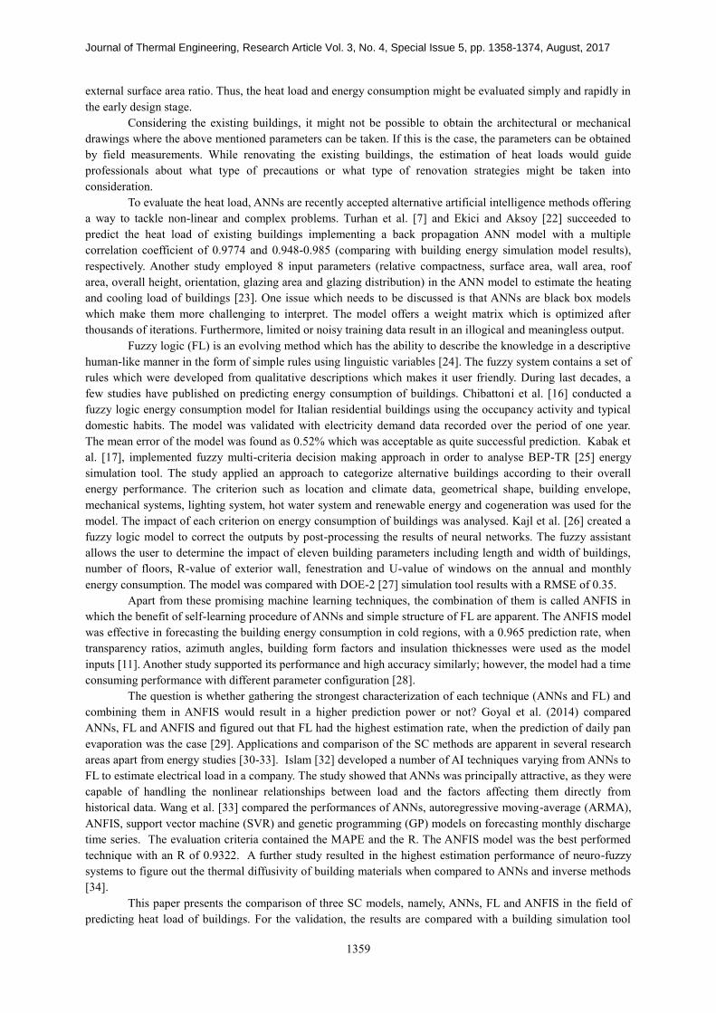
are distributed in scattered regions of the city. Figure 4 illustrates the schematic elevation and plan drawings of a
building which is four-storey high involving two separate apartments on each floor. The number of floors ranged
from 5 to 11, which directly provides information about the building form and its volume; while the orientation
covers every direction due to the city plan. Their zoning status which influences their total external wall area, is
either detached or attached on two sides. The data, on the other hand, correspond to the values of overall heat
transfer coefficient of the walls (U value), area-to-volume ratio (A/V), total external surface area (TESA), total
window area-to-total external surface area ratio (TWA/TESA) which are calculated and obtained the above
mentioned drawings. These are the most notable architectural parameters when the heat load has been calculated.
An example is summarized in Table 1.
The heat load values are gathered through simulations. The software named KEP-IYTE-ESS runs the
heat load calculations for each apartment, as explained in detail in previous studies [7 , 35, 44]. This monthly
static method including degree-day correction is based on the European standard EN ISO 13790 (2008) and the
Turkish standard TS 825. Its calculation process is validated and supported by BESTEST [45, 46]. The
performance of ANNs, FL and ANFIS depends on the comparison of soft computing findings with the ones
obtained from the software KEP-IYTE-ESS.
Development of SC methods
Three SC models were developed by employing original data from architectural projects. . In this study,
taking the data into consideration, the wall overall heat transfer coefficient (U), area/volume ratio (A/V), total
external surface area (TESA), total window area/total external surface area ratio (TWA/TESA). Although there
are several more parameters to obtain heat load of buildings, the parameters were chosen in this study are easily
measurable ones in case of architectural drawings of the buildings are not available which is the case for the
Table 1. Heating load characterization of one apartment
U value of the wall
(W/m2K)
TESA
(m2)
A/V
(1/m)
TWA/TESA
(-)
Heat Load
(kW/m2)
Apartment 1 1.43 213.66 0.4134 0.1636 0.0266
Apartment 2 1.37 1324.04 0.4001 0.1048 0.0425
Apartment 3 1.64 736.56 0.391 0.3016 0.0907
Journal of Thermal Engineering, Research Article Vol. 3, No. 4, Special Issue 5, pp. 1358-1374, August, 2017
1364
Figure 4. Schematic drawings of one residential building with two apartments on one floor
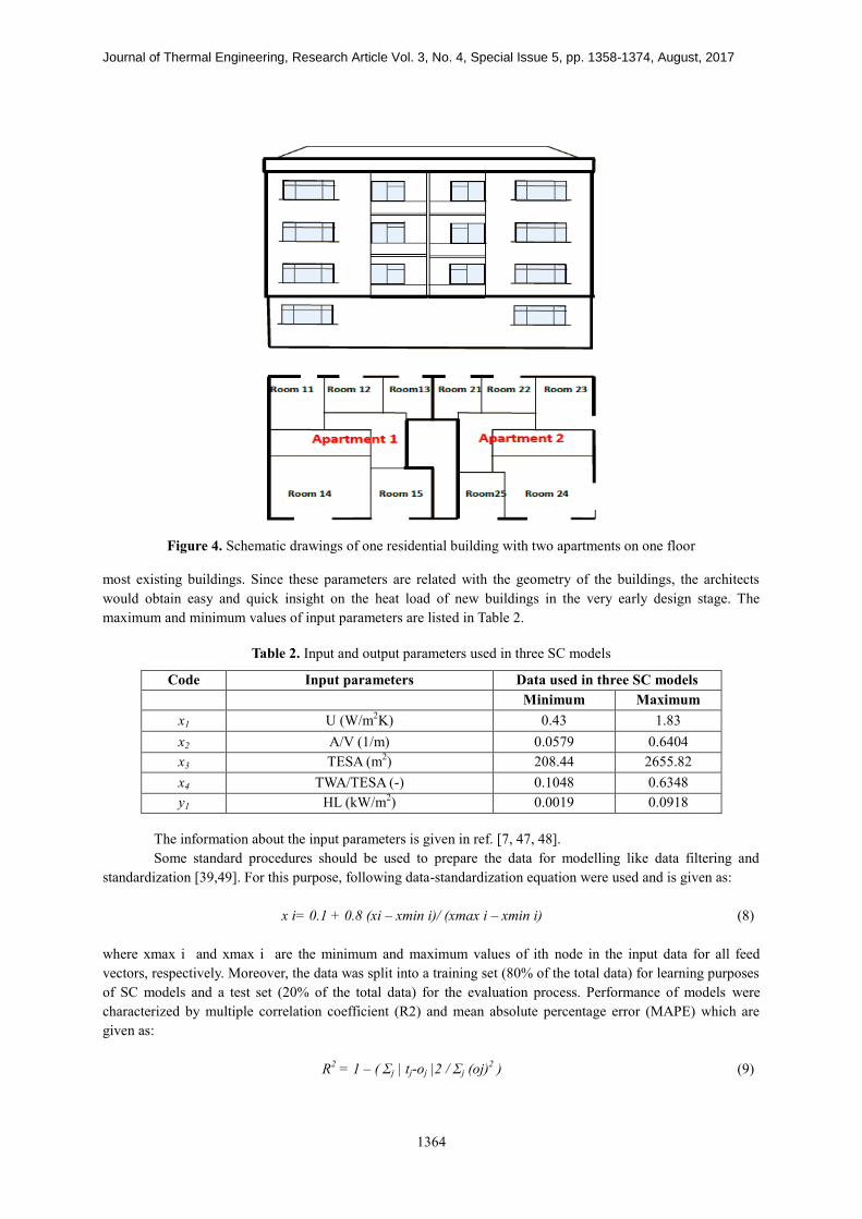
most existing buildings. Since these parameters are related with the geometry of the buildings, the architects
would obtain easy and quick insight on the heat load of new buildings in the very early design stage. The
maximum and minimum values of input parameters are listed in Table 2.
Table 2. Input and output parameters used in three SC models
Code Input parameters Data used in three SC models
Minimum Maximum
x1 U (W/m2K) 0.43 1.83
x2 A/V (1/m) 0.0579 0.6404
x3 TESA (m2) 208.44 2655.82
x4 TWA/TESA (-) 0.1048 0.6348
y1 HL (kW/m2) 0.0019 0.0918
The information about the input parameters is given in ref. [7, 47, 48].
Some standard procedures should be used to prepare the data for modelling like data filtering and
standardization [39,49]. For this purpose, following data-standardization equation were used and is given as:
x i= 0.1 + 0.8 (xi – xmin i)/ (xmax i – xmin i) (8)
where xmax i and xmax i are the minimum and maximum values of ith node in the input data for all feed
vectors, respectively. Moreover, the data was split into a training set (80% of the total data) for learning purposes
of SC models and a test set (20% of the total data) for the evaluation process. Performance of models were
characterized by multiple correlation coefficient (R2) and mean absolute percentage error (MAPE) which are
given as:
R2 = 1 – ( Σj | tj-oj |2 / Σj (oj)
2 ) (9)

Journal of Thermal Engineering, Research Article Vol. 3, No. 4, Special Issue 5, pp. 1358-1374, August, 2017
1365
MAPE = 1/p Σj [| (tj-oj) / tj|]*100 (10)
t is the target value, o is the output value and p is the number of input-output pairs [50]. Here, the R2 is expected
to be close to 1, while the MAPE should be as close as to zero for the best performance.
ANN model
ANN models were developed for the case buildings and published earlier in Ref [7]. The Levenberg–
Marquardt (LM) algorithm were used for the models with an iteration number of 20,000. The optimum structure
of the best ANN models was found to be 4-7-5-1 neuron in each layers. Learning rate was constant during the
prediction process and equal to 0.02. Log-sigmoid transfer function which is widely used for transfer function
was selected in the hidden layer and output layer. For further detail of ANN model structure please see Ref. [7].
FL model
FL approach is particularly useful in prediction problems due to its simplicity and natural structure. To
generate a simpler model, FL model was established including four inputs (U, A/V, TESA and TWA/TESA) and
an output (HL). Both Mamdani and Sugeno fuzzy inference systems (FIS) were developed for the study. The
fuzzy subsets of the variables were considered to have triangular and trapezoid membership functions. The
inference operator and defuzzification methods were selected as “the min” and “centroid” methods, respectively.
Three subdivisions of inputs and parameters namely were set as low (L), medium (M) and high (H) as
represented in Figure 5.
In the model, the fuzzy rules were expressed as “IF-THEN” format. Table 3 shows an example of 20
fuzzy rules set randomly from the total 81 rules.
Table 3. 20 fuzzy rules selected from the total of 81 sets
U value of the
wall (W/m2K)
A/V ratio
(m2/m
3)
TESA
(m2)
TWA/TESA
(-)
HL
(kW/m2)
L L L L VL
L L L H L
M L L L L
H L L L M
L L M M M
L M H L M
L L H H H
L L H L M
L M L L VL
L L H L L
L L H M M
H H M H VH
H L H M VH
H L L H H
M L L H H
M L M H H
H L M M VH
H M M H VH
H H L H H
H H H H VH
Let us assume that the U value of the wall is 0.8 W/m2K, A/V ratio is 0.30 m
2/m
3, TESA is 250 m
2 and
TWA/TESA is 0.2. We want to find out the fuzzy output of the heat load of the building under these variables
would be. As seen in Figure 5, 0.8 W/m2K is a part of “low” and “medium” subsets of the U value of the wall
with µ(U)=0.95 and µ(U)=0.05 membership degrees, respectively. Similarly, 0.3 of A/V ratio is a part of “low”
and “medium” subsets with membership degrees of µ(A/V)=0.05 and µ(A/V)=0.95, respectively. The fuzzy
inference engine would consider the following rules from the fuzzy rule base related to the above example and

Journal of Thermal Engineering, Vol. 3, No. 4, Special Issue 5, pp. 1358-1374, August, 2017 Yildiz Technical University Press, Istanbul, Turkey
1367
Figure 5. Block diagram used for fuzzy modeling

Journal of Thermal Engineering, Vol. 3, No. 4, Special Issue 5, pp. 1358-1374, August, 2017 Yildiz Technical University Press, Istanbul, Turkey
1368
IF U value of the wall is “low” (µ(U)=0.90), A/V ratio is “medium” (µ(A/V)=0.83), TESA is “low”
(µ(TESA)=0.98) and TWA/TESA is “low” (µ(TWA/TESA)=0.32) THEN the heat load of the building is “very
low” (µ(HL)= min (0.90, 0.83, 0.98,0.32)= 0.32.
IF U value of the wall is “low” (µ(U)=0.90), A/V ratio is “low” (µ(A/V)=0.17), TESA is “medium”
(µ(TESA)=0.02) and TWA/TESA is “medium” (µ(TWA/TESA)=0.68) THEN the heat load of the building is
“medium” (µ(HL)= min (0.90, 0.17, 0.02,0.68)= 0.02.
Figure 5 shows the output value of 0.0084 kW/m2 corresponding to 0.32 degree of membership in the
“very low” subset of the heat load of building and the output values of 0.0106 and 0.069 kW/m2 corresponding to
0.02 degree of membership in the “medium” subset of the heat load of building.
When one employs Eq. (7) for the above example, the following output value would be obtained by weighted-
average defuzzification;
heat load*= [0.32*(0.0084) + 0.02*(0.0106+0.095)/2]/ (0.32+0.02)
heat load*= 0.0102 kW/m2
ANFIS Model ANFIS approach have many benefits since it is the combination of ANN and FL approaches. To this
aim, an ANFIS model was developed with 300 epoch, 3-3-3 number of neurons and 81 fuzzy rules. Sugeno-type
ANFIS model with four inputs and an output was selected as the best performed model. The input membership
function was ‘gaussmf’ and the output membership function was ‘linear’. Table 4 depicts the used training
parameters in the ANFIS model for the heat load of buildings prediction.
Table 4. Training parameters of the ANFIS for the heat load
Parameters Heat load of buildings
Number of nodes 193
Number of linear parameters 405
Number of nonlinear parameters 24
Number of fuzzy rules 81
Membership function Gaussmf
Epoch 300
Output MF type Linear
Number of MF (input) 3-3-3
RESULTS AND DISCUSSION
Three SC models of existing residential buildings were developed for 4 input parameters which were U
value of the wall, A/V ratio, TESA and TWA/TESA ratio. The output parameter was the heat load of the
buildings. The input data was compiled from a total number of 148 residential building including 2136
apartments situated in Izmir. The developed models were applied to predict the heat load of buildings and
compare with the KEP-IYTE-ESS results. The commonly used statistical criteria mean absolute percentage error
(MAPE) and the multiple correlation coefficient (R2) were calculated to evaluate the performance of the models.
The comparison of KEP-IYTE-ESS and the best ANN model results of building heat load set is given in Figure
6a. The figures indicate that the model is able to give a successful prediction of 97.7% the MAPE of 5.06. Figure
6b depicts the comparison of KEP-IYTE-ESS and FL model results of building heat load set. From the figures, it
is evident that the FL model illustrates a reasonably good performance with R2 of 98.6%.
Mamdani method is widely accepted for capturing expert knowledge that allows us to describe the expertise in
more intuitive, more human-like manner. On the contrary, Sugeno method is computationally efficient and works
well with optimization and adaptive techniques, makes it very attractive in control problems, particularly for
dynamic non-linear systems. The most fundamental difference between Mamdani-type FIS and Sugeno-type FIS
is the way the crisp output is generated from the fuzzy inputs. Mamdani FIS has output membership functions
whereas Sugeno FIS has no output membership functions [51, 52]. Table 5 shows the comparison of two FIS
performances. The highest R2 of 98.6% and the lowest MAPE of 3.56% were obtained with Mamdani fuzzy
inference systems.
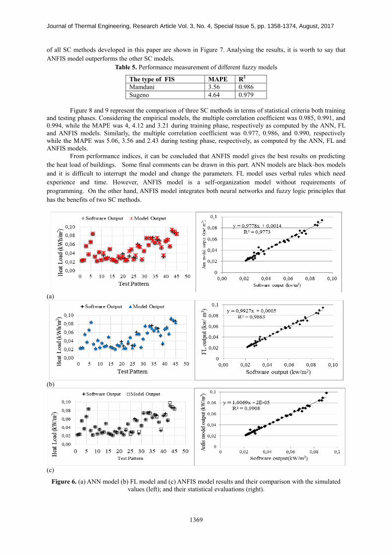
Figure 6c shows the comparison of ANFIS model and simulation results. The figures indicate that the
predicted values of the model had close match with the simulation software outputs (R2 of 99%). The comparison
Journal of Thermal Engineering, Research Article Vol. 3, No. 4, Special Issue 5, pp. 1358-1374, August, 2017
1369
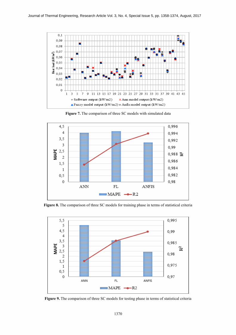
of all SC methods developed in this paper are shown in Figure 7. Analysing the results, it is worth to say that
ANFIS model outperforms the other SC models.
Table 5. Performance measurement of different fuzzy models
The type of FIS MAPE R2
Mamdani 3.56 0.986
Sugeno 4.64 0.979
Figure 8 and 9 represent the comparison of three SC methods in terms of statistical criteria both training
and testing phases. Considering the empirical models, the multiple correlation coefficient was 0.985, 0.991, and
0.994, while the MAPE was 4, 4.12 and 3.21 during training phase, respectively as computed by the ANN, FL
and ANFIS models. Similarly, the multiple correlation coefficient was 0.977, 0.986, and 0.990, respectively
while the MAPE was 5.06, 3.56 and 2.43 during testing phase, respectively, as computed by the ANN, FL and
ANFIS models.
From performance indices, it can be concluded that ANFIS model gives the best results on predicting
the heat load of buildings. Some final comments can be drawn in this part. ANN models are black-box models
and it is difficult to interrupt the model and change the parameters. FL model uses verbal rules which need
experience and time. However, ANFIS model is a self-organization model without requirements of
programming. On the other hand, ANFIS model integrates both neural networks and fuzzy logic principles that
has the benefits of two SC methods.
(a)
(b)
(c)
Figure 6. (a) ANN model (b) FL model and (c) ANFIS model results and their comparison with the simulated
values (left); and their statistical evaluations (right).
Journal of Thermal Engineering, Research Article Vol. 3, No. 4, Special Issue 5, pp. 1358-1374, August, 2017
1370
Figure 7. The comparison of three SC models with simulated data
Figure 8. The comparison of three SC models for training phase in terms of statistical criteria
Figure 9. The comparison of three SC models for testing phase in terms of statistical criteria

Journal of Thermal Engineering, Research Article Vol. 3, No. 4, Special Issue 5, pp. 1358-1374, August, 2017
1371
CONCLUSIONS
This paper explores the potential of the ANN, FL and ANFIS modelling techniques on the estimation of
the heat load of buildings. The input data are composed of basic architectural parameters, U value of the wall,
A/V ratio, TWA/TESA ratio and TESA, which are gathered from drawings of 2136 apartments located in Izmir-
Turkey. In general, the prediction of the heat load of building requires data on many input parameters. Further, it
involves non-linear equations whose solution is complex. The dynamic building energy simulation software
require detailed building and environmental parameters as input data which is possible only for the buildings
whose architectural projects are accessible and valid. As expected, existing input data, however, will lead to a
low accurate simulation. In addition, operating the simulation tools is difficult to perform and they normally
require expert users. Regression models generally use homogenous data sets and predictions are often done with
statistical software which are based on conventional algorithms such as curve fitting, the least square method and
time series. However, the flexibility of these models is limited by the formulation of the building parameters that
have non-linear relationships among each other. ANNs can solve non-linear and complex problems but they are
black box models. Besides, limited or noisy training data may result in an inconsistent and meaningless output in
some models. Fuzzy logic models are useful tools in the prediction of heat load of buildings where the building
and environmental parameters are unknown. Comparing the number of input data required for simulation
software, fuzzy logic models suggest a simple model with a high accuracy using limited input parameters.
However, the FL technique requires a significant time and experienced users to construct the verbal rules. ANFIS
model has the advantage of being significantly faster and more accurate than many ANN and FL models. The
results indicated that the SC models are powerful tools to estimate the heat load of buildings. Considering
statistical parameters, ANFIS model was the best model both in training and testing phases
Acknowledgements
The Scientific and Technological Research Council of Turkey (TÜBİTAK) funded this research and
their contribution is gratefully acknowledged (Project Number: 109M450).
NOMENCLATURE
ANFIS adaptive neuro-fuzzy inference system
AI artificial intelligence
ANNs artificial neural networks
ARMA autoregressive moving-average
A/V area/volume ratio (1/m)
bi Bias
CO2 carbon dioxide
FIS fuzzy inference system
FL fuzzy logic
GP genetic programming
HL heat load (kW/m2)
Kx* defuzzified output value
Kix output value in the ith
subset
LM levenberg-marquardt
MAPE mean absolute percentage error
MF membership function
MSE mean squared error
MSD mean squared deviation
netj net inputs
o desired output
p Pattern
R correlation coefficient
R2 multiple correlation coefficient
RMSE root mean squared error

Journal of Thermal Engineering, Research Article Vol. 3, No. 4, Special Issue 5, pp. 1358-1374, August, 2017
1372
SC soft computing
SVR support vector machine
t network output
TESA total external surface area (m2)
TWA/TESA total window area/ total external surface area
μ(Kix) membership value of the output value in the ith
subset
U wall overall heat transfer coefficient (W/m2K)
x1,x2,…..,xn scaler inputs
w1j,w2j,….wnj Weights
y Output
REFERENCES
[1] J.S. Hygh, J.F. DeCarolis, D.B. Hill, S.R.Ranjithan, Multivariate regression as an energy assessment tool in
early building design, Building and Environment 57 (2012) 165-175.
[2] I. Korolija, Y. Zhang, L.M. Halburd, V.I. Harby, Regression models for predicting UK office building energy
consumption from heating and cooling demand, Energy and Buildings 59 (2013) 214-227.
[3] T. Catalina, V.Iordache, B. Caracaleanu, Multiple regression models for fast prediction of the heating energy
demand, Energy and Buildings 57 (2013) 302-312.
[4] M.Manfren, N.Aste, R.Moshksar, Calibration and uncertainty analysis for computer models- A meta-model
based approach for integrated building energy simulation, Applied Energy 103 (2013) 627-641.
[5] Y.Heo, R. Choudhary, G. Augenbroe, Calibration of building energy models for retrofit analysis under
uncertainty, Energy and Buildings 47 (2012) 550-560.
[6] A. Boyano, P. Hernandez, O.Wolf, Energy demands and potantial savings in European office buildings: Case
studies based on EnergyPlus simulations, Energy and Buildings 65 (2013) 19-28.
[7] C.Turhan, T.Kazanasmaz, İ.Erlalelitepe Uygun, K.E.Ekmen, G.Gökçen Akkurt, Comparative study of a
building energy performance software (KEP-IYTE-ESS) and ANN-based building heat load estimation, Energy
and Buildings 85, 115-125.
[8] G. Mavromatidis, S. Acha, N.Shah, Diagnotic tools of energy performance for supermarkets using Artificial
Neural Network algorithms, Energy and Buildings 62 (2013) 304-14.
[9] S.K. Kwok, Y. E.W.M.Lee, A study of the importance of occupancy to bulding cooling load in prediction by
intelligent approach, Energy Conversion and Management 52 (2011) 2555-2564.
[10] Q. Li, Q.L. Meng, J.J. Cai, H. Yoshino, A. Mochida, Predicting hourly cooling load in the building: A
comparison of support vector machine and different artificial neural networks, Energy Conversion and
Management 50 (2009) 90-96.
[11] B.B.Ekici, U.T.Aksoy. Prediction of building energy needs in early stage of design by using ANFIS, Expert
Systems with Applications, 38 (2011) 5352-5358.
[12] K.Li, H. Su. Forecasting building energy consumption with hybrid genetic algorithm-hierarchical adaptive
network-based fuzzy inference system, Energy and buildings, 42 (2010), 2070-2076.
[13] F. Boithias, M. El Mankibi, P. Michel, Genetic algorithms based optimization of artificial neural network
architecture for buildings’ indoor discomfort and energy consumption prediction, Building Simulation 5 (2)
(2012), 95-106.
[14] S. A. Kalogirou, Artificial Neural Networks and Genetic Algorithms in Energy Applications in Buildings,
Advances in Building Energy Research 3 (1) (2009), 83-119.
[15] T.Kazanasmaz, Fuzzy logic model to classify effectiveness of daylighting in an office with a movable blind
system, Building and Environment, 69 (2013), 22-34.
[16] L. Ciabottoni, M.Grisostomi,G.Ippoliti, S.Longhi, Fuzzy logic home energy consumption modelling for
residential photovoltaic plant sizing in the new Italian scenario, Energy74 (2014), 359-367.
[17] M.Kabak, E.Köse, O.Kırılmaz, S.Burmaoğlu, A fuzzy multi-criteria decision making approach to access
building energy performance, Energy and Buildings 72 (2014), 382-389.
[18] C.Li, G.Zhang,M.Wang,J.Yi, Data-driven modelling and optimization of thermal comfort and energy
consumption using type-2 fuzzy method, Soft Computing 17 (2013), 2075-2088.

Journal of Thermal Engineering, Research Article Vol. 3, No. 4, Special Issue 5, pp. 1358-1374, August, 2017
1373
[19] Republic of Turkey ministry of energy and natural resources, Retrieved 05st March 2014,
fromhttp://www.enerji.gov.tr/yayinlar_raporlar_EN/ETKB_2010_2014_Stratejik_Plani_EN.pdf
[20] T. Kazanasmaz, İ.Erlalelitepe Uygun, G.Gökçen Akkurt, C.Turhan, K.E.Ekmen, On the relation between
architectural considerations and heating energy performance of Turkish residential buildings in Izmir, Energy
and Buildings 72 (2014) 38-50.
[21] H.X.Zhao, F.Magoules, A review on the prediction of building energy consumption, Renewable and
Sustainable Energy Reviews16 (3) (2012) 3586-3592.
[22] B.B.Ekici, U.T.Aksoy, Prediction of building energy consumption by using artificial neural networks.
Advanced Engineering Software 2011; 40: 356-362.
[23] J.S.Chou , D.K. Bui, Modelling heating and cooling loads by artificial intelligence for energy efficient
building design. Energy and Buildings 2014; 82: 437-446.
[24] G. Tayfur., S. Özdemir, P.V. Singh, Fuzzy logic algorithm for runoff-induced sediment transport from bare
soil surfaces, Advances in Water Resources 26 (2003), 1249-1256.
[25] National Building Energy Performance Calculation Methodology of Turkey. (No: YİG/2010-02)), Turkish
Official Journal (2010).
[26] S. Kajl, M.A. Roberge, L.Lamarche, P.Malinovski, Evaluation of building energy consumption based on
fuzzy logic and neural network applications, Proceedings of CLIMA 2000 conference (1997) 264-274.
[27] DOE- 2.2 Version 47d Edition, James J. Hirsch & Associates (JJH), 2009.
[28] K.Li, H.Su,J.Chu, Forecasting building energy consumption using neural networks and hybrid neuro-fuzzy
system: A comparative study, Energy and Buildings 43(10):2893-2899.
[29] M.K. Goyal, B. Bharti , J. Quilty , J. Adamowski, A. Pandey, Modeling of daily pan evaporation in sub-
tropical climates using ANN, LS-SVR, Fuzzy Logic, and ANFIS, Expert Systems with Applications 41 (2014),
5267–5276.
[30] M. Firat , Comparison of Artificial Intelligence Techniques for river flow forecasting. Hydrol. Earth Syst
2008;12: 123-129.
[31] A.K. Singh, M.C. Deo, S.V. Kumar, Neural network–genetic programming for sediment transport.
Proceeding of the ICE 2007; 160: 113-119.
[32] U.I.B. Islam, Comparison of Conventional and Modern Load Forecasting Techniques Based on Artificial
Intelligence and Expert Systems. IJCSI International Journal of Computer Science Issues 2011; 8 (5): 1694-
0814.
[33] C.W. Wang, W.K. Chau, C.T. Cheng, L. Qui, A comparison of performance several artificial intelligence
methods for forecasting monthly discharge time series. Journal of Hydrology 2009; 374: 294-306.
[34] S. Grieu , O.Faugeroux , O.Traure, B.Claudet, J.L. Bodnar, Artificial intelligence tools and inverse methods
for estimating the thermal diffusivity of building materials. Energy and Buildings 2011; 43:543-554.
[35] KEP-SDM. Dwelling Energy Performance-Standart Assessment Procedure, Chambers of Mechanical
Engineers. Izmir,Turkey. 2008.
[36] W. McCulloch, P. Walter, A Logical Calculus of Ideas Immanent in Nervous Activity. Bulletin of
Mathematical Biophysics 1943; 5 (4): 115–133.
[37] L.A. Zadeh, Fuzzy Logic = Computing with Words, IEEE TRANSACTIONS ON FUZZY SYSTEMS 4 (2),
1996, 103-111.
[38] T. Munakata, Fundamentals of the New Artificial Intelligence: Beyond Traditional Paradigms, Springer-
Verlag, New York, USA, 1998.
[39] G. Tayfur, Soft computing methods in water research engineering, WIT Press, Southampton, UK, 2012.
[40] S. Sivanandam , S. Sumathi, S. Deepe, “Introduction of Fuzzy Logic using MATLAB ,Springer, New York,
USA, 2007.
[41] A.D. Kulkarni, Computer Vision and Fuzzy-Neural Systems, Printice Hall, New Jersey, USA, 2001.
[42] K. Hirota, W. Pedrycz, Fuzzy logic neural networks: Design and computations, in: Proc. Int. Joint Conf.
Neural Networks Singapore (1991) 152-157.
[43] H.Esen, M. Inalli, A.Sengur, M. Esen, Predicting performance of a ground-source heat pump system using
fuzzy weighted pre-processing-based ANFIS, Building and Environment 43, 2008, 2178-2187.
[44] T. Kazanasmaz ,İ. Erlalelitepe Uygun , G. Gokcen Akkurt ,C. Turhan , K.E. Ekmen , On the relation
between architectural considerations and heating energy performance of Turkish residential buildings in Izmir.
Energy and Buildings 2014; 72 :38-50.

Journal of Thermal Engineering, Research Article Vol. 3, No. 4, Special Issue 5, pp. 1358-1374, August, 2017
1374
[45] J.Neymark , R. Judkoff , G. Knabe , H.T. Le, M. Durig , A.Glass et al. ,Applying the building energy
simulation test (BESTEST) diagnostic method to verification of space conditioning equipment models used in
whole-building energy simulation programs. Energy and Buildings 2012; 34, 917–931.
[46] G. Gokcen Akkurt, C.D. Sahin, S. Takan , Z.D. Arslan, Testing a simplified building energy simulation
program via building energy simulation test (BESTTEST). CLIMAMED 7th Mediterranean Congress of
Climatization October 2013: Istanbul, Turkey; 49–57.
[47] R.Pachedo, J.Ordonez, G.Martinez, Energy efficient design of building: A review, Renewable and
Sustainable Energy Reviews 16 (6) (2012) 3559-3573.
[48] L.P. Wang, J. Gwilliam, P. Jones, Case study of zero energy house design in UK, Energy and Buildings 41
(2009) 1215-1222.
[49] C.W.Dawson, R.Wilby, An artificial neural network approach to rainfall-runoff modelling, Hydrological
Sciences Journal 43 (1), 1998, 47-66.
[50] V.M.P. Antognetti. Neural Networks, Concepts Applications and Implementations. New Jersey, USA:
Prentice Hall;1991.
[51] A. Kaur, A. Kaur, Comparison of Mamdani-Type and Sugeno-Type Fuzzy Inference Systems for Air
Conditioning System, International Journal of Soft Computing and Engineering (IJSCE) 2 (2) (2012) 2231-2307.
[52] A. A. Shleeg, IM. Ellabib, Comparison of Mamdani and Sugeno Fuzzy Interference Systems for the Breast
Cancer Risk, Engineering and Technology International Journal of Computer, Information, Systems and Control
Engineering 7 (10) (2013) 695-699.