performance measurement of network applicationjharris/3comproject/masters... · performance...

i

Performance Measurement of Network Application

A Thesis

Presented to the Faculty of the

California Polytechnic State University

San Luis Obispo

In Partial Fulfillment

of the Requirement of the Degree

Master of Science in Computer Science

By

Siu Ming Lo

June 1999

ii

AUTHORIZATION FOR REPRODUCTION OF MASTER’S THESIS

I grant permission for the reproduction of this thesis in its entirety or any of its parts,

without further authorization from me.

__________________________________Signature

__________________________________Date

iii

APPROVAL PAGE

TITLE: Performance Measurement of Network Application

AUTHOR: Siu Ming Lo

DATE SUBMITTED: June 10, 1999

Dr. Mei-Ling Liu______________ ____________________________Advisor or Committee Chair Signature

Dr. Len Myers________________ ____________________________Committee Member Signature

Dr. Patrick Wheatley___________ ____________________________Committee Member Signature

iv

Abstract

Performance Measurement of Network Application

Siu Ming Lo

June 1999

During the past decade, the computer world has been undergoing a dramatic change in

many aspects. In the past, personal computer was known as a desktop machine that

functioned alone. All the resources, data, and computing power were within the same

machine. However, in the Internet world today, more and more computers are connected

together through the network to share data and resources or parallel the computation.

Networking Operation System (NOS) is the key technology to make this new computing

paradigm possible. One of the popular NOS is Windows NT 4.0, which was developed

by Microsoft Corporation. Meanwhile, many of networking software is developed to take

advantage of this emerging paradigm of computing. Efficient implementation of the

networking software is crucial to be competitive in the market. This study will investigate

an instrumentation technique which utilizes the Windows NT Performance Counters to

evaluate the performance of the networking software. The three major performance

metrics in which we are interested are CPU utilization, latency and throughput.

Keywords

Performance measurement, Performance Evaluation, Network application, File Transfer

Protocol, Windows NT Performance Counters, Performance Data Helper (PDH) library

v

Acknowledgments

I would like to express my sincere gratitude to my advisor, Dr. Mei-Ling Liu, for

her guidance, advice, motivation, assistance and patience throughout my course of

preparing this thesis. Without her help, I doubt I would be able to finish my thesis before

leaving Cal Poly.

I would also like to thank my thesis committee members, Dr. Len Myers and Dr.

Patrick Wheatley, for providing valuable inputs to improve this thesis work.

Last, but not least, I would like to thank our sponsor, 3com, for all their support.

vi

Table of Contents

Pages

List of Figures viii

List of Tables xii

Chapter 1: Introduction and Background of the Project 1

1.1 Brief Introduction of the Project1.2 Background of the Project1.3 Outline of the Thesis

Chapter 2: Introduction to Network Performance Measurement 3

2.1 The Initiative of Network Performance Evaluation2.2 Some Common Metrics to evaluate Network Performance

Chapter 3: Techniques and Tools for Performance Measurement 7

3.1 The Proper Procedure of Evaluating Network Performance3.2 Two Major Categories of Network Performance Benchmark Tools3.2.1 Transport-layer benchmarks3.2.2 Application-layer benchmarks3.3 Introduction to Some Common Benchmark Tools3.3.1 Hewlett Packard Netperf3.3.2 Novell Perform33.3.3 Windows NT Performance Monitor (PERFMON)

Chapter 4: Performance Monitoring on Windows NT 14

4.1 Measuring Performance by Using Windows NT Performance Counters4.1.1 Introduction to Windows NT Performance Counters4.1.2 The Process of accessing Windows NT Performance Counters4.2 Performance Data Helper (PDH) Library4.2.1 Introduction to Performance Data Helper Library4.2.2 PDH Library Overview4.2.2.1 Terminology4.2.2.2 PDH Functions and Structures

Chapter 5: Overview of File Transfer Protocol (FTP) 27

Chapter 6: Testbed Environment Setup and Configuration 30

6.1 Hardware description of computer systems on the testbed

vii

6.2 Software description of computer systems on the testbed6.3 FTP Sever Installation and Configuration

Chapter 7: Instrumentation and Overhead Analysis 35

7.1 Overview of Instrumentation7.2 Instrumentation Points Selection7.3 Two Instrumentation Approaches7.3.1 Commonplaces Between Two Instrumentation Approaches7.3.2 In-line Instrumentation7.3.3 Monitoring Process Instrumentation7.3.3.1 Communication Data Structure7.3.3.2 Modification of the Instrumentation Files7.3.3.3 Modification of the PDHTest Software7.4 Overhead Estimation and Analysis of the Two Instrumentation

Methods7.5 Performance Metrics and Their Limitation7.6 Instrumentation Procedure on WinSock-FTP (graphical-mode FTP)

and NcFTP (text-mode FTP)7.7 Limitations of Using the In-line Instrumentation Method and

Difficulties Encountered in the Instrumentation Process

Chapter 8: Instrumentation Results and Analysis 73

8.1 CPU utilization profile of the WinSock-FTP application8.2 CPU utilization profile of the NcFTP application8.3 Latency and throughput of the WinSock-FTP application8.4 Latency and throughput of the NcFTP application

Chapter 9: Conclusion and Future Work 115

Bibliography 117

Appendix A 119

viii

LIST OF FIGURES

Figure Page

1. Basic Configuration of Network System 5

2. Windows NT performance monitoring components interaction 16

3. The FTP model illustrates client and server with a TCP control connection 28

between them and a separate TCP connection between their associated

data transfer

4. The Testbed Setup for the Experiment 30

5. An instrumented WinSock-FTP application using In-line instrumentation 39

6. An instrumented WinSock-FTP application using monitoring process 40

instrumentation

7. Instrumentation code for both In-line Instrumentation and Monitoring 41

Process Instrumentation

8. The flow of execution of the instrumented WinSock-FTP application 43

9. The relationship and interaction between instrumented WinSock-FTP 48

and modified PDHTest application

10. The time-event diagram of instrumented WinSock-FTP and modified 49

PDHTest application

11. In-line instrumentation overhead estimation 62

12. Monitoring Process Instrumentation overhead estimation 62

13. A sample of performance data written to the text file 68

14. Verification of CPU utilization performance data 69

15. Reduction on the frequency of probing by interleaving 70

16. Overall CPU utilization profile of the WinSock-FTP application in 74

the file-sending operation

17. A detailed view of hotspot "A" (CPU utilization profile of the WinSock-FTP 76

application in the file-sending operation)

18. A detailed view of hotspot "B" (CPU utilization profile of the WinSock-FTP 77

ix


19. A detailed view of hotspot "C" (CPU utilization profile of WinSock-FTP 79


20. Overall CPU utilization profile of the WinSock-FTP application in the 80

file-receiving operation

21. A detailed view of hotspot "A" (CPU utilization profile of the 82

WinSock-FTP application in the file-receiving operation)

22. A detailed view of hotspot "B" (CPU utilization profile of the 83


23. A detailed view of hotspot "C" (CPU utilization profile of the 84


24. Overall CPU utilization profile of the NcFTP application in the 85

file-sending operation

25. A detailed view of hotspot "A" (CPU utilization profile of the NcFTP 87


26. A detailed view of hotspot "B" (CPU utilization profile of the NcFTP 88


27. A detailed view of hotspot "C" (CPU utilization profile of the NcFTP 89


28. A detailed view of hotspot "D" (CPU utilization profile of the NcFTP 90


29. Overall CPU utilization profile of the NcFTP application in the 91

file-receiving operation

30. A detailed view of hotspot "A" (CPU utilization profile of the NcFTP 92

application in the file receiving operation)

31. A detailed view of hotspot "B" (CPU utilization profile of the NcFTP 93

application in the file-receiving operation)

32. A detailed view of hotspot "C" (CPU utilization profile of the NcFTP 94


33. A detailed view of hotspot "D" (CPU utilization profile of the NcFTP 95


x

34. A detailed view of hotspot "E" (CPU utilization profile of the NcFTP 96


35. The latency of the WinSock-FTP application for sending file in the 97

range of 100 to 4000 bytes

36. The latency of the WinSock-FTP application for sending file in the 99

range of 100 to 1000 kilobytes

37. The throughput of the WinSock-FTP application for sending file in the 100


38. The throughput of the WinSock-FTP application for sending file in the 101


39. The latency of the WinSock-FTP application for receiving file in the 102


40. The latency of the WinSock-FTP application for receiving file in the 103


41. The throughput of the WinSock-FTP application for receiving file in 105

the range of 100 to 4000 bytes

42. The throughput of the WinSock-FTP application for receiving file in 106

the range of 100 to 2000 kilobytes

43. The latency of the NcFTP application for sending file in the range of 107

100 to 4000 bytes

44. The latency of the NcFTP application for sending file in the range of 108

100 to 4000 kilobytes

45. The throughput of the NcFTP application for sending file in the range 109

of 100 to 4000bytes

46. The throughput of the NcFTP application for sending file in the range 110

of 100 to 4000 kilobytes

47. The latency of the NcFTP application for receiving file in the range of 111

100 to 4000 bytes

48. The latency of the NcFTP application for receiving file in the range of 112

100 to 4000 kilobytes

49. The throughput of the NcFTP application for receiving file in the range 113

xi

of 100 to 4000 bytes

50. The throughput of the NcFTP application for receiving file in the range 114

of 100 to 4000 kilobytes

xii

LIST OF TABLES

Table Page

1. IP addresses and hardware addresses of computer systems on the testbed 31

13

Chapter 1: Introduction and Background of the Project

1.1 Brief Introduction of the Project

The Windows NT Performance Monitor (PERFMON) has been widely recognized by

application developers as a useful tool for debugging and performance evaluation during

the process of development. However, it has some shortcomings that will be mentioned

later. The goal of this project is to demonstrate a technique using Performance Counters

to measure Windows NT network performance. Application-level instrumentation is the

main focus. We will use a File Transfer Protocol (FTP) application as an example of

network software for proof of concept. Instrumentation approaches, experimental results,

analysis and conclusion will be presented. The primary goal (or motivation) behind the

project is to investigate and demonstrate the feasibility of employing NT Performance

Counters provided by the Windows NT operating system to obtain valid performance

data such as latency and CPU utilization. Also, the result and experience attained will

provide insight on the feasibility of using this technique to instrument the Windows NT

TCP/IP stack.

1.2 Background of the Project

This study is funded by 3Com-CalPoly joint research project, which was initiated in

January 1997. The primary goal of this joint project focuses on the “Maximization of

Network Performance”. In the Electrical Engineering building, Room 104, Faculty

Research Laboratory, a Local Area Network (LAN) with five NT workstations,

contributed by 3com, has been specifically set up for this research project. Research and

study activities have been ongoing since the lab was operative. Some of these activities

14

include reviews of computer architecture, reviews of CPU/memory and network caching

literature, studies of network performance measurement and tools, studies of parallel

network processing, development of the prototype I2O network-disk interface process,

and so on. The joint project has supported many undergraduate student senior projects

and graduate student master theses.

1.3 Outline of the Thesis

This thesis is organized as follows. In Chapter 2, we give an introduction of network

performance measurement. In Chapter 3, we describe the techniques and tools for

performance measurement. An introduction to Windows NT performance monitoring and

the Performance Data Helper (PDH) library are presented in Chapter 4. Chapter 5

provides some basic knowledge of the File Transfer Protocol (FTP). Chapter 6 contains

information on the setup of the tested environment and its configuration. In Chapter 7, we

describe our instrumentation approaches and the instrumentation overhead analysis. In

Chapter 8, we discuss our instrumentation results and analysis. Finally, we present

conclusions in Chapter 9.

15

Chapter 2: Introduction to Network Performance Measurement

The necessity to evaluate the performance of computer systems has been recognized for a

long time [12]. Performance measurement has been significantly important to computer

system designers, administrators, and analysts to justify the impact of a new design or

change compared to existing system. On the other hand, this information is also

important to the users or customers to evaluate different systems from different vendors

to determine whether their needs can be fulfilled.

Svobodova [12] categorizes system evaluations into two major trends: comparative

evaluations and analytic evaluations. Comparative evaluation compares the performance

of two or more systems with same set of system parameters and workload model. The

purpose of this evaluation is to compare the efficiency and effectiveness of different

products or services. On the other hand, analytic evaluation studies the performance of a

single system with respect to various system parameters and/or system workload. The

purpose of this evaluation approach is to optimize the performance of a system.

2.1 The Initiative of Network Performance Evaluation

A computer network, or even the Internet, is composed of dozens to thousands or even

millions of computers connected together. The goal is to allow information and valuable

resources to be shared among computers located at different sites. As the usage of the

Internet exploded in mid 90s, more and more communication software applications and

distributed applications (which take advantage of parallel processing to achieve high

throughput and performance) will be developed and deployed over the Internet or

16

corporate networks. Therefore, the importance of network performance measurements is

accentuated by the rapid deployment of these network software applications in this

decade.

As Liu mentioned [1], “ Network system performance is the performance of a computer

system where networking plays a significant (if not the dominant) role, hence it is a

continuum of computer system performance.” Computer system performance studies

have already been around for a long time. In traditional computer performance

evaluation, the subject is a single computer comprised of hardware and software

components. Most concerns are concentrated on the comparison of performance between

two or more computer system or optimization of performance of a single system. On the

other hand, the network system is a product of the combination of the computer

technology with the networking technology, whereby independent computers are

interconnected through a network. With this approach, independent computers are able to

share resources including CPU cycles, data, applications, and services among others. For

a network system, also known as distributed system, the scope of performance evaluation

is considerably extended and complicated by the existence of the network component.

Not only is the performance of individual systems an issue, but the interaction among the

computers as well as the network which interconnects them also play a significant role.

This additional dimension of the network increases the difficulty and amount of effort on

evaluating such a system significantly compared with evaluating a traditional, standalone

computer system.”

17

The following diagram illustrates the basic configuration of network system.

Network OperatingSystem A

Network OperatingSystem B

NetworkProtocol Stack

NetworkProtocol Stack

Network InterfaceCard

Network InterfaceCard

Network Media (Wire)

Application A

Application B

Application C

Application D

2.2 Some Common Metrics to evaluate Network Performance

As Svobodova[12] phrased it: “The very fundamental problem of computer performance

analysis is the problem of defining ‘performance’ and of defining criteria for performance

evaluation. First, it must be understood that performance is a qualitative characteristic,

highly subjective to the needs of the people involved with the system meets the

expectation of the person involved with it.”

Figure 1 Basic Configuration of Network System

18

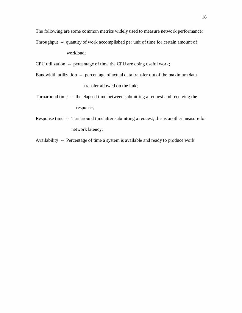
The following are some common metrics widely used to measure network performance:

Throughput -- quantity of work accomplished per unit of time for certain amount of

workload;

CPU utilization -- percentage of time the CPU are doing useful work;

Bandwidth utilization -- percentage of actual data transfer out of the maximum data

transfer allowed on the link;

Turnaround time -- the elapsed time between submitting a request and receiving the

response;

Response time -- Turnaround time after submitting a request; this is another measure for

network latency;

Availability -- Percentage of time a system is available and ready to produce work.

19

Chapter 3: Current techniques or tools for performance measurement

The subject of network performance evaluation has been of concern for a long time,

especially in industry. Currently, one of the most popular evaluation techniques,

benchmarking, is widely employed by vendors and users of network equipment and

systems, and by independent parties providing network performance evaluation.

3.1 The Proper Procedure of Evaluating Network Performance

The process of network performance measurement [1] generally follows the steps

described below. A valid scheme or model should cover all of these steps.

1. Define and implement a model that closely represents the system to be evaluated, also

known as the system model.

2. Define and implement the workload of the system. The workload model should truly

reflect the amount and the type of work the system is expected to do.

3. Define performance metrics to be used for the evaluation.

4. Design and implement a performance monitoring mechanism that allows

measurements to be observed and recorded.

5. Obtain the values of the chosen performance metrics.

6. Interpret the measurements with respect to system performance.

By definition, a benchmark is “a point of reference from which measurements can be

compared [1].” In terms of computer performance evaluation, a benchmark usually

means “a job or a set of jobs that represents a typical workload for a computer system,

which could be a single instruction, a program, or a specified sequence of function calls.”

20

How well the benchmark to approximate the real system workload is determined by how

proper the mix of jobs representative of each class of applications in the actual workload.

In other words, a benchmark is like a simulator, which generates the effect of the usage of

system resources. However, the benchmark commonly referred to in existing literature on

network performance is actually more than a workload generator, it also includes a

performance monitor. The performance monitor component is a collection of modules

that allows the performance of the evaluated system to be observed, measured, recorded,

and interpreted.

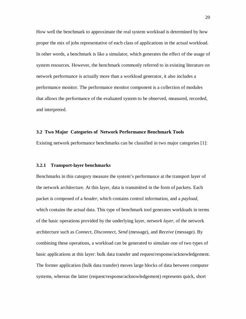
3.2 Two Major Categories of Network Performance Benchmark Tools

Existing network performance benchmarks can be classified in two major categories [1]:

3.2.1 Transport-layer benchmarks

Benchmarks in this category measure the system’s performance at the transport layer of

the network architecture. At this layer, data is transmitted in the form of packets. Each

packet is composed of a header, which contains control information, and a payload,

which contains the actual data. This type of benchmark tool generates workloads in terms

of the basic operations provided by the underlying layer, network layer, of the network

architecture such as Connect, Disconnect, Send (message), and Receive (message). By

combining these operations, a workload can be generated to simulate one of two types of

basic applications at this layer: bulk data transfer and request/response/acknowledgement.

The former application (bulk data transfer) moves large blocks of data between computer

systems, whereas the latter (request/response/acknowledgement) represents quick, short

21

exchanges of messages. For bulk data transfer applications, the primary performance

measure of interest is throughput; for request/response applications, it is response time.

Hewlett Packard Netperf [13] is an example of a Transport-layer benchmark.

3.2.2 Application-layer benchmarks

Another class of network performance benchmarks are those which measure the

performance at the application layer, where the basic operations are more abstract than

those at the transport layer. At this layer, the workload is perceived in terms of files being

transferred between a client and a server or in terms of requests being fulfilled by a

server. There are two sub-types, divided along the line of two popular applications of

network systems: file serving and transaction serving. In file-serving applications, the

data of one or more files is transferred between a client and a server. In transaction-

serving applications, a client requests a service (such as for data from a database) and the

request is processed by the server. For the former, the measure of the most interest is the

throughput of files being transferred. For the latter, it is the response time, the time

between when a request is issued and when the response is received. Novell Perform3 is

an example of an Application-layer benchmark.

3.3 Introduction to Some Common Benchmark Tools

The followings are three common benchmark tools that have been commonly used in

industry:

22

3.3.1 Hewlett Packard Netperf

Netperf [13] is a benchmark that can be used to measure various aspects of networking

performance. Its primary focus is on bulk data transfer (throughput) and request/response

(response time) performance using either TCP or UDP and the Berkeley Sockets

interface. There are optional tests available to measure the performance of DLPI, Unix

Domain Sockets, the Fore ATM API and the HP HiPPI LLA interface.

Netperf [13] is designed around the basic client-server model. There are two executables

- netperf and netserver. Generally you will only execute the netperf program - the

netserver program will be invoked by the other system's inetd.

When you execute netperf, the first thing that will happen is the establishment of a

control connection to the remote system. This connection will be used to pass test

configuration information and results to and from the remote system. Regardless of

the type of test being run, the control connection will be a TCP connection using BSD

sockets. Once the control connection is up and the configuration information has been

passed, a separate connection will be opened for the measurement itself using the APIs

and protocols appropriate for the test. The test will be performed, and the results will

be displayed.

Netperf can also be used to measure CPU utilization except this is a difficult metric to

measure accurately. By default, Netperf uses a technique, which are tight loops

consuming any CPU cycles left over by the networking, then calculates the difference

23

between the total number of CPU cycles and the CPU cycles consumed by the loops. The

CPU utilization is presented as a percentage of the total number of CPU cycles.

3.3.2 Novell Perform3

Perform3 [7], a benchmark developed by Novell, is a client/server benchmark. It

measures the network adapter throughput produced by memory-to-memory data transfers

from a file server to the participating client workstation. It measures throughput by

reading block size files from the server’s cache. It uses the file server’s disk caching as

this ensures that there is no server disk activity during the read. The delay in the server

disk’s read and write would otherwise hinder performance measurements. This also

enables the network adapter cards to perform at their peak. Perform3 reads the cached file

for a specified number of seconds and then calculates the throughput in kilobytes per

second.

Perform3 can be used to measure individual workstations or a group of workstations. If

more than one workstation is used, Perform3 is initiated on one workstation, which is

selected as the master workstation. After the master workstation is established then

Perform3 is run on all the other workstations under test. The start of each test is

coordinated through the master workstation so that all the workstation tests start at the

same time. Perform3 collects all test data at the end of the run and generates an aggregate

number in kilobytes per second for the entire test.

24

3.3.3 Windows NT Performance Monitor (PERFMON)

PERFMON is a built-in tool for monitoring the performance of Windows NT computer

systems. It is a tool that is diverse and customizable and is regularly used in industry to

obtain performance analysis. One of its main characteristics is that it can be customized

to report measurements required by the vendor. One of its uses in the industry is in

testing the performance of device drivers and providing a good feedback on making

design decisions. Its performance monitoring utility is based on an object-based model.

System components such as drivers and services export various performance objects,

whose attributes can then be imported by PERFMON. In Windows NT an object is a

standard mechanism for identifying and using system resources. Objects are created to

represent individual processes, sections of shared memory, and physical devices. Disk

drives, adapter cards, and processes are just a few examples of the performance objects

supported by PERFMON. Data are collected for each of the performance objects in the

form of performance counters. These counters can then be used to compute a wide

variety of measurements. PERFMON also supports object instances of each object type.

A complete set of counter instances are assigned to each of the object instances, so

performance measurements can be collected on each of the object instances. All the

measurements on performance objects are collected and displayed in a graphical

presentation. PERFMON provides charting, alerting, and reporting capabilities that

reflect both current activity and ongoing logging.

25

However, based on our observation, PERFMON has at least the following 3 limitations:

1. Performance data are displayed at a fixed rate of once per second.

2. It does not provide a mechanism to capture data at a specific instrumentation point.

3. It does not provide timing information between pairs of instrumentation points.

26

Chapter 4: Performance Monitoring on Windows NT

In spite of its usefulness and ease-to-use user interface, PERFMON suffers the limitations

mentioned in the previous section. This prompted us to look for alternatives to

compensate the deficiencies, but without scarificing the powerful performance

monitoring capability provided by PERFMON. One of the solutions we propose is to use

Windows NT Performance Counters. NT Performance Counters use the same mechanism

to collect and retrieve performance data information from NT Internal as PERFMON. A

detailed description will be given in Section 4.1. However, this approach seems more

fulfilled the requirements in terms of higher rate of data probing and data collection at a

specific instrumentation point. Generally, NT Performance Counters will be accompanied

by Performance Data Helper (PDH) Library functions, which provide an interface to

simplify the access to the NT Performance Counters’ internal structure, to access

performance data information. More detailed descriptions of PDH Library functions will

be given in section 4.2.

4.1 Measuring Performance by Using Windows NT Performance Counters

4.1.1 Introduction to Windows NT Performance Counters

The performance data that the Windows NT operating system provides contains

information for a variable number of object types, instances per object, and counters per

object type. Detailed descriptions of these terminologies will be given in the section

4.2.2.1. The counters are used to measure various aspects of performance. For example,

the Process object includes the Handle Count counter to measure the number of handles

open by the process. An instance is a unique copy of a particular object type, though not

27

all object types support multiple instances. For example, the System object has no

instances since there is only one System. On the other hand, the Process object supports

multiple instances because Windows NT supports multiple processes.

In order for a program to utilize the performance features of the Windows NT operating

system, the use of the Registry functions is necessary. The Registry functions retrieve

groups of data from the HKEY_PERFORMANCE_DATA key that contains the

performance information. The blob of data is formatted according to specifications that

are documented in the Platform SDK (Software Development Kit)[2]. Section 18.4 of

“The Windows NT Device Driver Book”, Art Baker [4], also has a detail description on

the overall structure of performance data such as PERF_DATA_BLOCK,

PERF_OBJECT_TYPE, PERF_COUNTER_DEFINITION, PERF_COUNER_BLOCK,

and PERF_INSTANCE_DEFINITION structures. We must also be aware of how to

perform the calculations on this raw data in order to get the information we would expect

from a counter. There are around 30 different types of counters that can be in the

performance data, so there are 30 different ways to calculate the information.

(Technically there are fewer, since some of the counter types share the same calculation

method.)

4.1.2 The Process of accessing Windows NT Performance Counters

Performance information [4] (performance counter -- data about a given performance

object) for Windows NT is not stored in the Registry in the same way that hardware or

software configuration data is. Rather, the Win32 Registry function calls gather

28

performance data at the time someone asks for it, which could be triggered by a PDH

(Performance Data Helper) library function call. The following diagram shows all the

components behind the scene, which demonstrates how Windows NT Performance

Counters can be accessed by PDH library functions

File MappingObject

DeviceControl

User-modeDriver

Kernel-modeDriver

PDH LibraryFunction Call

Data Collection DLL

Win32 RegistryAPI

The following describes the sequence of events that occur when we run an application

program to access system performance data [4].

1. The application uses the Win32 RegQueryValueEx function to access the

HKEY_PERFORMANCE_DATA key.

Figure 2 [4] Windows NT performance monitoring components interaction

29

2. The Registry API scans HKEY_LOCAL_MACHINE\…\Services for drivers and

services with a Performance subkey, which identifies a driver or service as a

performance monitoring component. Values contained in the Performance subkey

identify a data-collection DLL that acts as an interface between the Registry API and

the objects being monitored.

3. The Registry API maps these interface DLLs into the process requesting performance

data. It then calls the Open and Collect functions in each DLL to determine what

objects and counters the DLL supports.

4. Each time the application want updated performance information, it calls the

RegQueryValueEx again. This results in calls to the Collect function in each

performance component’s data-collection DLL. The Collect function gets a raw

sample from the object being monitored and sends it back to PDH library function.

5. When the application closes the HKEY_PERFORMANCE_DATA key with

RegCloseKey, the Registry API calls the DLL’s Close function to do any necessary

cleanup. It then unmaps the DLL from the process.

4.2 Performance Data Helper (PDH) Library Interface

In Windows NT, the easiest way to obtain the performance data is to use the Performance

Monitor available in the Administrative Tools group. However, if we need to collect

30

performance data for our application, the easiest way to do this is to use the interface

provided by the Performance Data Helper (PDH) library. Applications that need more

control over performance data collection can use the registry interface directly. This is the

method that is used by the functions in PDH.DLL and by the Performance Monitor. It is

more efficient for the Performance Monitor to use the registry interface, because it

displays counters grouped by object. If you are retrieving individual counters, rather than

a group of counters from a particular object, it is just as efficient to use the PDH

interface.

4.2.1 Introduction to Performance Data Helper Library

The Performance Data Helper (PDH) is a companion library to the native performance-

monitoring features of the Windows NT operating system. It is built on top of the

standard performance-monitoring features of Windows NT and doesn't really add any

new functionality to native performance monitoring.

What the PDH Library does is to package the data in a form that does not require any

traversal at all. As a matter of fact, the library also provides a nice dialog box that allows

the user to select counters interactively. You can use the library without the dialog box

simply by specifying counters as strings. For instance, the counter for a Process object's

Handle Count is specified as a string that looks like this: \Process(MyApp)\HandleCount.

This simplification is at the heart of the PDH Library. It is not necessary to know

anything about the native performance data in order to easily find the information we

seek.

31

4.2.2 PDH Library Overview

4.2.2.1 Terminology

Objects/Object Type

An Object Type is defined as a measurable entity. The term object is also used to refer to

a measurable entity. The list of objects on our system includes Browser, Cache, ICMP,

IP, Logical Disk, Memory, NBT Connection, Network Interface, NWLink IPX, NWLink

NetBIOS, NWLink SPX, Objects, Paging File, Physical Disk, Process, Processor,

Redirector, Server, Server Work Queues, System, TCP, Telephony, Thread, and

UDP.

Each of these objects is associated with a different set of counters. For instance, the

Physical Disk object has counters that measure disk performance while the Memory

object has counters that measure memory performance.

Counter

A counter is unit of performance. It provides data related to a single item of the system.

Some examples of counters are Handle Count and Thread Count, both associated with a

Process object. Another counter is the % Processor Time, which measures the amount of

processor time an object utilizes. This counter is actually used in two different Object

types, a Process object and a Thread object. In a Process object, the % Processor Time

counter measures the entire process, while % Processor Time for a Thread object

measures only a specific thread.

32

Instance

An instance is an instantiation of a particular object, such as a specific process or thread.

All instances of a given Object have the same set of counters. For example, the Process

object has an instance for each of the running processes. The Thread object has an

instance for each thread of each process in the system. As mentioned earlier, some

objects, like the Memory object don't have instances at all since there is always only one

of them in the system. Some objects may have zero instances, which means that there are

no current instantiations of the object. This can occur, for instance, in the Telephony

object if Telephony has never been configured.

The above definitions are not really related to the PDH Library directly since they are

part of the native performance data; however, we must understand them in order to use

the PDH Library properly. The following definitions, however, are specific to the PDH

Library.

Counter name string

A counter name string is of special importance to the PDH Library, since this is the

identifier of a counter for inclusion in gathering performance data. The counter names

must be formatted a specific way in order to be properly recognized by the PDH Library.

The format is:

\\Machine\PerfObject(ParentInstance/ObjectInstance#InstanceIndex)\Counter

33

The \\Machine portion is optional. If included, it specifies the name of the machine. If a

machine name is not included, the PDH Library uses the local machine.

The \PerfObject component is required; it specifies the object that contains the counter. If

the object supports variable instances, then you must also specify an instance string. The

format of the (ParentInstance/ObjectInstance#InstanceIndex) portion depends on the type

of object specified. If the object has simple instances, then the format is just the instance

name in parentheses. For example, an instance for the Process object would be the

process name such as (Explorer) or (MyApp).

The \Counter portion is required; it specifies the performance counter. A more detailed

explanation on Counter can be found in the Counter section above.

Fortunately, the PDH Library supplies a counter browsing dialog box that will build the

counter name strings automatically. This allows us to avoid having to know everything

about the counter name strings before we can use the PDH Library. Platform SDK

documentation [2] has format specification of the counter path string.

Query

A query is a collection of counters. The PDH Library supports multiple queries. For

instance, we could have a query that contains counters related to one process, and another

query that contains counters related to another process. Each of these queries can be

individually updated to gather the raw data associated with each counter in the query.

34

Additionally, we could have a query containing counters for which frequent updates are

required and another query containing counters for which infrequent updates are needed.

Multiple queries allow this flexibility.

Our program creates queries. Once created, they can be used in PDH functions to update

the counters they contain. Counters are also added to a query by our program. If we do

not add any counters to a query, then nothing interesting will occur.

Raw data

Raw data are the data that is associated with a counter as it appears in the native

Windows NT performance data. There is little that can be done with the raw data,

although they are important for statistical calculations.

Formatted data

Formatted data in the PDH Library are data that we expect to see from a counter. The

PDH Library formats the data for us based on the calculations that are required depending

on the counter type in the native Windows NT performance data. We do not have to

know anything about these calculations or how they work in order to get properly

formatted data from the counters.

Statistics

The PDH Library also handles statistical calculations for us. The library provides

statistics on average, minimum, and maximum for each counter we specify. Proper

35

calculation of statistics requires that a collection of raw data be kept for some time

period. It is up to our application to save the raw data in a queue and update this

information as often as necessary.

Browse Performance Counters Dialog and Callback Function

The PDH Library provides a dialog box that allows the user to interactively select

counters for monitoring. This dialog box allows the user to select an object. When an

object is selected, the list of counters changes to show the counters that are relevant for

the selected object. Also, instances are shown if the object has instances.

There are many ways to modify the behavior of the dialog box. For instance, one may

only want to add only a single counter per dialog box or to allow counters from remote

machines to be added.

A callback function is associated with the dialog that allows your program to be notified

when the user chooses to add a counter. The callback function is executed and all selected

counters are reported to the function. The callback function is responsible for actually

doing something with the selected counters. If the callback function does nothing, then

the selection has no effect. Obviously, for anything interesting to occur, the callback

function must add the counter to a query.

36

4.2.2.2 PDH Functions and Structures

The prototypes and structure definitions for the PDH functions come in two header files.

The header file PDH.h must be included in order to gain access to the functions, data

types, and structure definitions used in the PDH Library.

All of the PDH functions have a return type of PDH_STATUS. The actual values we can

expect from the functions are defined in the PDHMsg.h header file. We must include this

header file in order to use the definitions described in the documentation.

To properly link to the PDH Library, we must use the PDH.LIB import file that comes

with the Platform SDK [2].

The following introduce some of the most common PDH library functions used for

performance data collection:

To create a query and start using the PDH Library, call the PdhOpenQuery function. This

function takes a pointer to a HQUERY variable as one of its parameters. This HQUERY

variable will contain the handle to the query created. Remember that a query is a

collection of counters, so after PdhOpenQuery, the query is initially empty.

To close a query, call PdhCloseQuery, passing the HQUERY for the query you wish to

close.

37

In the PDH Library, counters are more than just the performance data. Counters also have

status and a timestamp.

To add a counter to a query, you must call the PdhAddCounter function. You supply the

HQUERY associated with the counter you are adding and also supply the counter name

string. You can optionally supply some user data (a 32-bit value) to associate with the

counter. The function takes a pointer to a HCOUNTER variable. If the function is

successful, then this HCOUNTER variable will contain the handle to the counter.

To remove a counter from a query, call PdhRemoveCounter, passing the HCOUNTER for

the counter you wish to remove.

The counter name string can come from any number of sources. Either the counter string

is stored in a file, or hard coded in the program. You can also use the PDH Browse

Performance Counters dialog box to allow the user to interactively select counters to add.

In any case, once a counter name is determined, you must call PdhAddCounter in order to

get the counter added to a query.

To collect performance data, call PdhCollectQueryData function collects the current raw

data value for all counters in the specified query and updates the status code of each

counter. If the function succeeds, it returns ERROR_SUCCESS. If the function fails, the

return value is a PDH error status defined in pdhmsg.h. However, the

PdhCollectQueryData function can succeed, but may not have collected data for all

38

counters. Therefore, we should always check the status code of each counter in the query

before using the data.

After performance data has been collected, we need to display it in a readable format. We

call PdhGetFormattedCounterValue function, which returns the current value of a

specified counter in the format requested by the caller. There are three possible formats

can be specified in the parameter by the caller. PDH_FMT_DOUBLE returns data as a

double-precision floating point real. PDH_FMT_LARGE returns data as a 64-bit integer.

PDH_FMT_LONG returns data as a long integer.

39

Chapter 5: Overview of File Transfer Protocol (FTP)

In this project, we choose File Transfer Protocol (FTP) [6][7] as an implementation

example of network application to demonstrate our concept. Therefore, it may be

appropriate to briefly introduce the File Transfer Protocol (FTP).

File transfer is among the most frequently used TCP/IP applications, and it accounts for

much network traffic. Standard file transfer protocols existed for the ARPANET before

TCP/IP became operational. These early versions of file transfer software evolved into a

current standard known as the File Transfer Protocol (FTP).

FTP runs on top of a reliable end-to-end transport protocol like TCP. Besides file

transfer, FTP also offers many other facilities. For example,

1. Interactive Access.

2. Format (representation) Specification.

3. Authentication Control.

Like other servers, most FTP implementations allow concurrent access by multiple

clients. Clients use TCP to connect to the server. A single master server process awaits

connections and creates a slave process to handle each connection. Unlike most servers,

however, the slave process does not perform all the necessary computation. Instead, the

slave accepts and handles the control connection from the client, but uses an additional

process or processes to handle a separate data transfer connection. The control connection

40

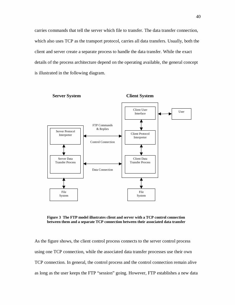
carries commands that tell the server which file to transfer. The data transfer connection,

which also uses TCP as the transport protocol, carries all data transfers. Usually, both the

client and server create a separate process to handle the data transfer. While the exact

details of the process architecture depend on the operating available, the general concept

is illustrated in the following diagram.

Client UserInterface

Client ProtocolInterpreter

Client DataTransfer Process

Server ProtocolInterpreter

Server DataTransfer Process

FileSystem

FileSystem

User

Control Connection

Data Connection

FTP Commands& Replies

Server System Client System

As the figure shows, the client control process connects to the server control process

using one TCP connection, while the associated data transfer processes use their own

TCP connection. In general, the control process and the control connection remain alive

as long as the user keeps the FTP “session” going. However, FTP establishes a new data

Figure 4 The FTP model illustrates client and server with a TCP control connectionFigure 3 The FTP model illustrates client and server with a TCP control connectionbetween them and a separate TCP connection between their associated data transfer

41

transfer connection for each file transfer. In fact, many implementations create a new pair

of data transfer processes, as well as a new TCP connection, whenever the server needs to

send information to the client. Once the control connection disappears, the session is

terminated and the software at both ends terminates all data transfer processes.

When a client forms an initial connection to a server, the client uses a random, locally

assigned, protocol port number, but contacts the server at a well-known port (21). Many

clients can contact a server with this scheme, because TCP uses both endpoints to

identify a connection. When the control processes create a new TCP connection for a

given data transfer, the client obtains an unused port on its machine and uses it to contact

the data transfer process on the server’s machine. The data transfer process on the server

machine can use the well-known port reserved for FTP data transfer (20). To ensure that

a data transfer process on the server connects to the correct data transfer process on the

client machine, the server side must not accept connections from an arbitrary process.

Instead, when it issues the TCP passive open request, it specifies the port that will be

used on the client machine as well as the local port.

42

Chapter 6: Testbed Environment Setup and Configuration

Experiments of this study are conducted in Cal Poly – 3Com joint project laboratory

located at building 20, room 114. This laboratory is also known as Faculty Resources

Laboratory. The following figure shows the network testbed topology.

R100b3129.65.26.70

(Source machine)

R100b2129.65.26.23

(Target machine)

Outlander129.65.26.67(NT server)

100BaseT

Fast Ethernet

Instrumented FTPapplication isinstalled here

Figure 4 The Testbed Setup for the Experiment

43

Machine Name IP Address Hardware Address

(Ethernet Address)

Outlander

(Windows NT Server)

129.65.26.67 00:60:97:2d:b1:a7

R100b2

(Passive host machine)

129.65.26.23 00:60:97:2d:b1:d9

R100b3

(Target machine)

129.65.26.70 00:60:97:2d:b1:e0

Table 1 IP addresses and hardware addresses of computer systems on the testbed

6.1 Hardware description of computer systems on the testbed

Outlander

• HP Netserver LH Pro

• Dual Intel X86 family 6 Model 1 Stepping 7 Processors

• 3Com Fast EtherLink XL PCI 10/100 Adapter (3C905)

• HP 4.26GB A 80 LXPO Hard Drive

R100b2

• HP Vectra VL series 4 Pentinum 200MHz

• 32 Megabyte RAM


44

• Matrox Millenuim 2MB Video Card

• Quantum Fireball TM2 2.4GB Hard Drive

• Hitachi CDR-7930 CD-ROM

R100b3

• HP Vectra VL series 4 Pentinum 200MHz

• 96 Megabyte RAM


• Matrox Millenuim 2MB Video Card

• Quantum Fireball TM2 2.4GB Hard Drive

• Hitachi CDR-7930 CD-ROM

• Iomega Internal Zip Drive

6.2 Software description of computer systems on the testbed

The following only describes the major software have been used for this project.

R100b2 and R100b3

• Windows NT 4.0 Workstation with Service Pack 3

• Microsoft Visual Studio 97 Professional Edition

• Microsoft Office 97 Professional Edition

• Windows NT Software Development Kit (SDK)

• Windows NT Device Driver Kit (DDK)

45

• Microsoft Development Network (MSDN) Library - January 1999

• Intel’s VTune 3.0

• Network General’s NetXRay International Version 3.0.3

Outlander

• Windows NT 4.0 Server

6.3 FTP Server Installation and Configuration

By default, FTP server is not installed automatically while we install Windows NT 4.0

Workstation on our computer. In order to perform FTP experiments for this project, one

need to install it separately. A subscription to the Microsoft Developer Network package

has been provided for the CalPoly-3Com joint research project to regularly update our

development software such as SDK and DDK. Inside that package, FTP server software

can be found in Disk 4 with the title ”Windows NT 4.0 Workstation”. Once the CD is

found, one can start the installation.

The following describes the installation procedure of the FTP server.

1. Press the Start button on the lower, left-handed corner in the Windows environment,

select Settings and then select Control Panel.

2. Click on the Network icon and select the Services tab on the panel.

3. Look for Microsoft Peer Web Server from the Network Services list. If found, it

means the FTP server has been installed previously. Then one can skip the rest of

46

procedure and jump to configuration procedure below. If not found, click on Add

button.

4. Look for Microsoft Peer Web Server from the Network Services list in the Select

Network Service panel, highlight it and then press OK.

5. Put the CD into the CD-ROM, modify the driver letter of the path in the Window NT

Setup panel if necessary and then press Continue.

6. The necessary files for setting up the FTP server will be copied to the system.

After the FTP server software has been installed, one needs to go through the following

configuration procedure.

1. Press the Start button on the lower, left-handed corner in the Windows environment,

select Microsoft Peer Web Services (Common) and then select Internet Service

Manager.

2. Highlight the FTP service of the local computer, click on Properties menu and select

Start Service. This will change the FTP server into the running mode.

3. Then one can start to transfer file using anonymous access.

47

Chapter 7: Instrumentation and Overhead Analysis

7.1 Overview of Instrumentation

Instrumentation is a method used to collect and extract useful information from a subject.

This technique is widely employed in many different fields, especially in engineering and

technical industries. One simple example of using instrumentation is to determine the

temperature and pressure change of hot water while it flows along a long steel pipe.

In order to obtain the information, we need to attach thermometers and barometers to a

few locations along the pipe, so that we can monitor the change from one location to the

other. In this example, the hot water in the long steel pipe is our subject. The

thermometer and barometer are our instrumentation tools. The locations where the

thermometers and barometers are attached are instrumentation points. Temperature and

pressure are our parameters of measurement.

In this project, we measure the performance of one network software, File Transfer

Protocol (FTP), which runs on the Windows NT 4.0 platform. In this case, our subject is

48

the File Transfer Protocol (FTP) application. Our instrumentation tool is the

instrumentation code that accesses the NT Performance Counters. Details will be

discussed in section 7.3. In section 7.2, we will discuss how we choose our

instrumentation points. And in section 7.4, we will present the overhead estimation of the

instrumentation. In section 7.5, we will discuss what parameters we use as our

performance metrics. Then in section 7.6, we will describe the instrumentation procedure

for a WinSock-FTP application and an NcFTP application. Finally, limitations of using

the In-line instrumentation method and difficulties encountered in the instrumentation

process will be presented in section 7.7.

In the following discussion, there are two terms to which we are frequently referred.

Their meanings are defined as follows.

1. Instrumentation code – a small piece of C programming code that is inserted to the

source files of the target application under test. It indicates the location where we are

interested in collecting performance data. The details are discussed in Section 7.3.1.

2. Instrumentation files – a pair of files we wrote. Their file names are SimplePerf.h and

SimplePerf.c respectively. They provide an interface for performance data collection.

7.2 Instrumentation Points Selection

Where to insert instrumentation codes is crucial to attain meaningful results. This

decision is driven by the purpose of our instrumentation, which in this case, is the

information we expect to obtain from the application we instrumented. In this project, we

are interested in collecting performance information for an FTP application while it

49

performs some network-related operations. The operations to be evaluated are sending a

local file and retrieving a remote file. We decided to insert our instrumentation codes

along the execution path of those two operations. The following sums up the major points

of interest for our instrumentation. However, their exact function names are not presented

because they are dependent on the specific implementation of FTP.

(i) Start the FTP application

(ii) Connect to the remote host machine (input username and password)

(iii) Open the control connection

(iv) Open the data connection

(v) Transfer file (either sending or receiving)

(vi) Close the data connection

(vii) Close the control connection

(viii) Close the FTP application

7.3 Two Instrumentation Approaches

In terms of instrumentation methods, we had two distinct approaches at the beginning.

We intended to use both approaches for our experiments and to compare the outcomes.

The goal is to find out which method generates more accurate results. We use WinSock-

FTP as a target application for our instrumentation experiments.

50

In the first approach, we insert all the instrumentation to the WinSock-FTP application.

Once the flow of execution of the program reaches an instrumentation point, the

performance data collection operation will be performed within the WinSock-FTP

application. The instrumented WinSock-FTP is not interrupted from running while the

data is collected. In the second approach, we only insert part of the instrumentation to the

WinSock-FTP. When an instrumentation point is reached, performance data collection is

performed externally by an independent application, PDHTest. The instrumentation in the

WinSock-FTP application provides the interface that allows the two processes to

coordinate their operations. For instance, when the flow of execution reaches an

instrumentation point in the instrumented WinSock-FTP, it is interrupted from running

and passes control to the PDHTest. Then, the PDHTest starts to collect performance data.

Once it is finished, the PDHTest is interrupted and passes control back to the

instrumented WinSock-FTP until the next instrumentation point is reached. This

operation repeats continuously until the performance data of all the instrumentation

points has been collected.

51

The following diagram shows a screen shot of an instrumented WinSock-FTP application

(First Instrumentation Approach).

52

Figure 5 An instrumented WinSock-FTP application using In-line instrumentation

The following diagram shows a screen shot of an instrumented WinSock-FTP application

monitoring by PDHTest application (Second Instrumentation Approach)

53

Figure 6 An instrumented WinSock-FTP application using monitoring process instrumentation

7.3.1 Commonalties Between the Two Instrumentation Approaches

There are a few commonalties between two instrumentation methods. First of all, they

both use the same instrumentation code. The following shows a section of

instrumentation code directly copied from our instrumented WinSock-FTP application.

// get the start timettStart=time(NULL);

//*******************#ifdef DIRECT

PDH_GetData("Begin_recvthefile"); In-line instrumentation

54

pCount++;#endif//*******************//*******************#ifdef SHARE

PDH_GetData("Begin_recvthefile");#endif//*******************

// loop to receive input from remote endwhile(!bAborted && (iNumBytes=recv(sockfd,(LPSTR)szMsgBuf,4000,0))>0){

Figure 7 Instrumentation code for both In-line Instrumentation and Monitoring ProcessInstrumentation

We inserted both types of instrumentation code at the same instrumentation point. Since

they are put between the #ifdef - #endif statements, we can select either as our

instrumentation method by compiling the files with the corresponding identifier, either

DIRECT or SHARE. PDH_GetData is a data-collection function defined in our

instrumentation file. We will discuss it in details in section 7.3.2 and 7.3.3. pCount is a

integer variable to store the current count of the temporary data structure defined below.

Secondly, both instrumentation methods defer to print the performance data to the text

file until all the data have been collected from the instrumentation points. This approach

is for the accuracy of our instrumentation. In theory, the execution time of

instrumentation code should be as short as possible. The more time it takes, the more

inaccuracy it introduces. Since file operation is a very slow operation, it is unacceptable

to print the performance data to the file at every instrumentation point. Therefore, we

decided to store the performance data into an array of temporary data structures during

the process of data collection and then write the result back to a text file when the

collection is finished. Both instrumentation methods use the same temporary data

structure, which is shown below, to store the performance information.

Monitoring application

55

typedef struct Data{

char location[30]; // location stampULONG tCount; // time stampdouble counter1; // % processor timedouble counter2; // % user timedouble counter3; // % privileged time

} performData;

This temporary data structure stores performance information, which includes location,

time, percentage of processor time, percentage of user time, and percentage of privileged

time, at an instrumentation point.

7.3.2 In-line Instrumentation

In the first approach, besides inserting instrumentation code at the instrumentation points,

we include an additional pair of instrumentation files, SimplePerf.h and SimplePerf.c, to

the source code of WinSock-FTP application. Their function is to provide the

instrumented code an interface to access the performance data in the Windows NT

Performance Counters. Then we re-compiled the files, which include instrumentation

files and instrumentation-embedded WinSock-FTP source files, into an executable file,

an instrumented WinSock-FTP application. We named this approach In-line

instrumentation.

The following diagram shows the flow of execution of the instrumented WinSock-FTP

application.

Performancedata collection

WinSock-FTPInstrumentation files

56

In the instrumentation file, SimplePerf.c, we defined three functions. They are

(i) PDH_Start, (ii) PDH_GetData, and (iii) PDH_End respectively. As mentioned

before, their function is to provide the instrumented code an interface to access the

performance data in the Windows NT Performance Counters.

The following describes the responsibility of the three functions in detail:

BOOL PDH_Start(){

BOOL fRes = TRUE;int i;

szCounterName[0] = "\\Processor(0)\\% Processor Time";szCounterName[1] = "\\Processor(0)\\% User Time";szCounterName[2] = "\\Processor(0)\\% Privileged Time";

if(ERROR_SUCCESS != PdhOpenQuery(NULL, 1, &hQuery)){

fRes = FALSE;}

for (i=0; i<3; i++){

if(ERROR_SUCCESS != PdhAddCounter(hQuery, szCounterName[i] , 1,&hCounter[i]))

{

1

2

3

Figure 8 The flow of execution of the instrumented WinSock-FTP application

57

fRes = FALSE;

}}

return fRes;}

(i) PDH_Start is an initialization function. This function only needs to be called

once at the beginning of each run before we can start to collect performance data.

(1) At the beginning, it defines the performance counters we are interested in

monitoring into an array of counter name. (2) Then it calls a function in the PDH

library named PdhOpenQuery, which initiates a query and allows performance

counters be added to the query subsequently. If the call succeeds, a handle is

returned for this specific query. (3) After that, it invokes PdhAddCounter, another

PDH library function, to add all the counters defined in our array previously to the

query. Then we are ready to collect performance data.

BOOL PDH_GetData(char* nString){

BOOL fRes = TRUE;int i;LARGE_INTEGER hpCount;char *lpString = nString;

if(ERROR_SUCCESS != PdhCollectQueryData(hQuery)){

fRes = FALSE;}

for(i=0; i<3; i++){

if(ERROR_SUCCESS != PdhGetFormattedCounterValue(hCounter[i],PDH_FMT_DOUBLE, NULL, &pdhFormattedValue[i]))

{fRes = FALSE;

}

}

if(fRes != FALSE){

for(i=0; i<strlen(nString); i++){

dataArray[pCount].location[i] = *lpString;

3

2

1

58

lpString++;}dataArray[pCount].location[i] = '\0';

if(QueryPerformanceCounter(&hpCount))dataArray[pCount].tCount = (ULONG) (hpCount.QuadPart);

dataArray[pCount].counter1 = pdhFormattedValue[0].doubleValue;dataArray[pCount].counter2 = pdhFormattedValue[1].doubleValue;dataArray[pCount].counter3 = pdhFormattedValue[2].doubleValue;

}

return fRes;}

(ii) PDH_GetData is a data collection function. (1) It takes a single string as

argument. At each instrument point, we pass in a label, which represents this

particular instrumentation, as an argument. This is the key to associate a specific

instrumentation point with its performance data for the analysis. (2) Inside the

function, first of all, it calls a PDH library function, PdhCollectQueryData, to

update the performance information of all the counters defined in its query.

However, the performance information collected by this function is in raw data

format. (3) In order to present the data in a format that the user can understand,

another PDH library function, PdhGetFormattedCounterValue, needs to be

called. This function converts the raw data into either one of three displayable

formats, which are double-precision floating point real, 64-bit integer or long

integer. (4) QueryPerformanceCounter is another PDH library function that

allows us to query the time information of the system. It is called to keep a time

record so that the latency between two successive calls to PDH_GetData

function, which also represent the latency between two successive instrumentation

points, can be determined. Finally, all the information, including the label of the

instrumentation point, the time stamp, and the performance information of the

three counters, are copied to a temporary data structure for deferred printing.

4

59

BOOL PDH_End(){


for(i=0; i<3; i++){

if(ERROR_SUCCESS != PdhRemoveCounter(hCounter[i])){

fRes = FALSE;}

}

if(ERROR_SUCCESS != PdhCloseQuery(hQuery)){

fRes = FALSE;}

return fRes;}

(iii) PDH_End is a clean-up function. It is necessary to formally remove all the

performance counters from the query when the data-collection process is

completed. (1) It can be achieved by calling the PDH library function,

PdhRemoveCounter. It takes a handle to the query as parameter to remove all the

counters within it. (2) After that, another PDH library function, PdhCloseQuery,

is called to close the query. Then the clean-up procedure is completed.

7.3.3 Monitoring Process Instrumentation

In the second approach, in addition to inserting instrumentation codes at the

instrumentation points and including instrumentation files with the WinSock-FTP

application source code as in the first approach, we run an independent, monitoring

application, PDHTest, concurrently with the instrumented WinSock-FTP application.

PDHTest is a performance monitoring tool that comes with Windows NT 4.0. Its source

code is freely available and fully commented. Its function is to provide the instrumented

code an interface to access the performance data in the Windows NT Performance

Counters. This is the approach employed by the NT Performance Monitor. Another

1

2

60

performance monitor which adopts this approach is Statlist, which comes with SDK.

However, some changes on PDHTest application must be made in order to collect

performance data for the instrumented WinSock-FTP application. Also, the function of

instrumentation files, SimplePerf.h and SimplePerf.c, are different from the previous

instrumentation approach. They are only responsible for providing a synchronization

mechanism Event between the two processes, instrumented WinSock-FTP and PDHTest,

and for allocating a section of shared memory for their communication. A detailed

description of the change of instrumentation files and modification of PDHTest

application will be given in section 7.3.1. The following diagram shows the relationship

and interaction between the instrumented WinSock-FTP and the modified PDHTest

application.

61

Instrumentation code



InstrumentedWinSock-FTP

Application

PerformanceData Collection

SharedMemory

ModifiedPDHTest

Application

Instrumentation files

The access to the sharedmemory is synchronizedby the Windows NT built-in synchronizationmechanism Event

Temporarydata structure

The following shows the time-event diagram of the instrumented WinSock-FTP and

PDHTest application during the process of data collection.

The processis running

The processis waiting

InstrumentedWinSock-FTP

Application

ModifiedPDHTest

Application

Latencyintroduced by theinstrumentation

code

Time spent ondata collection

Figure 9 The relationship and interaction between instrumented WinSock-FTP andmodified PDHTest application

Figure 10 The time-event diagram of instrumented WinSock-FTP and modified PDHTestapplication

62

7.3.3.1 Communication Data Structure

In this approach, we use an independent, monitoring process for our data collection. In

order for the monitoring process to know where the data should be taken, we need to

provide a mechanism that allows the two processes, instrumented WinSock-FTP and

PDHTest, to synchronously communicate with each other. As mentioned before, the

function of the instrumentation files is to provide a synchronization mechanism Event and

to allocate a section of shared memory for communication. In the context of this

instrumentation method, shared memory is like a single-slot mailbox, which holds a

message for either of the two processes. On the other hand, Event is like the mail key.

The two processes need to get the key before they can open the mailbox to read the

message from or write the message to each other. This mechanism enforces the two

processes to run alternatively. Also, the message must be in a format that both processes

can understand. Therefore, we defined a data structure to accomplish this need.

struct sData{

BOOL doneFlag;int nextProcess;char location[SIZE];

};

This data structure is composed of three fields:

1. The first field is a Boolean variable named doneFlag. This variable signifies whether

the process of data collection has finished. By default, it is false. It can be set true

only by the PDH_End function, a clean-up function, of the instrumentation file. This

63

is how the PDHTest is notified to stop data collection and start the clean-up

procedure.

2. The second field is an integer variable named nextProcess. This variable indicates

which process schedule to run next. We used FTP_App, which is defined at a value of

10, to represent the instrumented WinSock-FTP and PDH_App, which is defined at a

value of 20, to represent the PDHTest. When a process gets the control, it first checks

this field to determine whether it is supposed to run. If it is, it will continue.

Otherwise, it will release the control to let another process an opportunity to run. This

mechanism enforces the two processes to run alternatively.

3. The last field is a character string variable named location. This variable is used by

the instrumented WinSock-FTP to pass the label information of instrumentation

points to PDHTest. Therefore PDHTest can associate the label with the performance

data it collects.

The information of this data structure is copied to the section of shared memory, on

which both processes are mapped. Therefore, they both can read from and write to this

shared memory for communication in a coordinated manner.

7.3.3.2 Modification on Instrumentation Files

In this approach, we also need to include additional instrumentation files to the source

code of WinSock-FTP. However, as mentioned in section 7.3, their functions are only

responsible to provide a synchronization mechanism between the two processes,

64

instrumented WinSock-FTP and modified PDHTest, and allocate a section of shared

memory for their communication. The following is the details of the three functions.

BOOL PDH_Start(char* nString){

BOOL fRes = TRUE;int i;BYTE *lpSharedData = &sharedData;DWORD errCode = 0;char *lpString = nString;

sharedData.doneFlag = FALSE;sharedData.nextProcess = PDH_App;


sharedData.location[i] = *lpString;lpString++;

}sharedData.location[i] = '\0';

// A sort of creating a mutexhEvent = CreateEvent(NULL, TRUE, FALSE, "accessToken");

// create a chunk of shared memory for communicationhFileMapObj = CreateFileMapping((HANDLE)0xFFFFFFFF, NULL,

PAGE_READWRITE, 0, 0x00000100, "sMemory");

/ map to that chunk of shared memorylpMapView = MapViewOfFile(hFileMapObj, FILE_MAP_READ |

FILE_MAP_WRITE, 0, 0, 0);

// copy everything in sharedata struct into shared memorylpSharedData = &sharedData;for(i=0; i<sizeof(sharedData); i++){

lpMapView[i] = (BYTE)*lpSharedData;(BYTE)lpSharedData++;

}

// release it, so others can grab itretValue = SetEvent(hEvent);

return fRes;}

(i) PDH_Start is an initialization function. (1) It first initializes the communication

data structure with proper values. For example, it sets the doneFlag variable to be

false; it also sets the nextProcess variable to be PDH_App, which means that

PDHTest is the next process to run; and finally it stores the label of

instrumentation point in the location variable. (2) Then it invokes a

1

2

3

4

5

6

65

synchronization mechanism called Event, which can be accomplished by calling a

Microsoft Windows NT 4.0 (WinNT4) library function named CreateEvent. This

function takes a unique name, which is accessToken in our case, as one of the

arguments and returns a handle to this event. The unique name identifies this

particular Event object. Later, if another process opens an Event with the same

name, both processes will be able to use this built-in mechanism to synchronize

themselves. (3) After that, it calls another WinNT4 library function,

CreateFileMapping, to allocate a section of shared memory. This function is

similar to CreateEvent function and takes a name, which is sMemory, to uniquely

identify the allocated shared memory. Similarly, if another process uses WinNT4

OpenFileMapping function to open shared memory with the same name, both

processes will be able to use this to communicate with each other. (4) However,

before the process can use this section of shared memory, it needs to call another

WinNT4 library function, MapViewOfFile, to map its view to this shared

memory. (5) Then it copies all the information from the communication data

structure onto the shared memory. (6) Finally, it sets the Event by calling

WinNT4 SetEvent function. This function notifies all other processes, which

subscribe to this Event object, that the process holding the Event object has

suspended and given up the control (the Event object). Any other processes

waiting for this Event object have the opportunity to get a hold on it and start to

run.



66

BYTE *lpSharedData = &sharedData;char *lpString = nString;

while (1){

WaitForSingleObject(hEvent, 1000);

retValue = ResetEvent(hEvent);

lpSharedData = &sharedData;lpSharedData += sizeof(BOOL);for(i=0; i<sizeof(int); i++){

(BYTE)*lpSharedData = lpMapView[sizeof(BOOL)+i];(BYTE)lpSharedData++;

}

if(sharedData.nextProcess == FTP_App)break;

retValue = SetEvent(hEvent);}

//**********************// Copy the location and time stamp to shared memory here//**********************





lpSharedData = &sharedData;for(i=0; i<sizeof(sharedData); i++){


}

retValue = SetEvent(hEvent);

return fRes;}

(ii) PDH_GetData is a function that updates the label of the instrumentation point

and signals the PDHTest to collect performance data. At the beginning, it enters

an infinite loop. (1) Inside that loop, it waits for the Event, which is accessToken,

to be set by some processes using a WinNT4 library function,

WaitForSingleObject. (2) Whenever it responds to the Event, it resets the Event

immediately by calling ResetEvent, another WinNT4 library function. What it

5

4

3

2

1

67

does is to mark that the Event is not available anymore. (3) Then it copies the

information to the communication data structure and checks the nextProcess field

to determine whether this process is supposed to run. If it is, it exits the infinite

loop and continues. Otherwise, it sets the Event, stays in the loop and waits for the

Event again. (4) After exiting the loop, it sets the doneFlag field of the data

structure to be false, assigns the nextProcess field with PDH_APP and copies the

label of the instrumentation point to the location field. (5) Finally, it copies the

information of the data structure back to the shared memory and sets the Event.

Then it finishes the process of updating PDHTest the current label of the

instrumentation point.

BOOL PDH_End(char* nString){

BOOL fRes = TRUE;int i;BYTE *lpSharedData = &sharedData;char *lpString = nString;

// this while-loop check to make sure who's turn. If not, release the controlwhile(1){

WaitForSingleObject(hEvent, 1000);retValue = ResetEvent(hEvent);



}


retValue = SetEvent(hEvent);//** might put delay here **

}

//**********************

1

68

// Copy the location and time stamp to shared memory here//**********************

// Copy back the new stuff into the shared memorysharedData.doneFlag = TRUE;sharedData.nextProcess = PDH_App;






}


// this while-loop check to make sure who's turn. If not, release the controlwhile(1){


lpSharedData = &sharedData;

lpSharedData += sizeof(BOOL);for(i=0; i<sizeof(int); i++){


}


retValue = SetEvent(hEvent);}

UnmapViewOfFile(lpMapView);

CloseHandle(hFileMapObj);

return fRes;}

(iii) PDH_End is a clean-up function. (1) First of all, it enters the infinite loop as

PDH_GetData function does. It keeps checking until it has permission to run. (2)

After exiting the loop, it sets the doneFlag field to be true to notify PDHTest of

the end of the data collection process, assigns the nextProcess field with

PDH_APP and copies the label of the instrumentation point to the location field.

2

3

4

69

Then it copies back the information to the shared memory and sets the Event. This

signifies to the PDHTest to end the data collection and start its own clean-up

procedure. (3) Then it enters an infinite loop again. It waits for PDHTest to finish

the above tasks and pass the control back. (4) Once the control is back, it finally

removes its view from the shared memory and de-allocates it.

7.3.3.3 Modification on PDHTest Software

Also, some modifications need to be made on PDHTest software so that it can

synchronously communicate with the instrumented WinSock-FTP application. Most of

the changes are made in a function called AutoStart. Originally, there is only a single line

of code that requests performance data to be collected once per second. We have changed

that to collect data at the instrumentation points. We substituted the original code with

our code. (1) Similar to PDH_Start at the beginning, it calls a WinNT4 library function,

OpenEvent, and uses the same name, which is accessToken, as argument. By doing this,

both modified PDHTest and instrumented WinSock-FTP use the same Event object to

synchronize themselves. (2) Then it calls another WinNT4 library function,

OpenFileMapping, to open up the same section of shared memory allocated by the

instrumented WinSock-FTP previously. It is accomplished by providing the same name,

which is sMemory, as the argument to the function. (3) After that, another WinNT4

library function, MapViewOfFile, is called to map a view of the shared memory into the

address space of the calling process. Thereafter, similar to PDH_GetData, it enters the

double infinite loops. (4) The function of the inner infinite loop is to continuously check

whether this process, modified PDHTest, should run before it continues. (5) After exiting

70

the inner loop, it copies all the information from the shared memory to the

communication data structure and then invokes the function collectData, which we

defined, to collect the performance data and stores in the temporary data structure. (6)

Then it checks the doneFlag field of the communication data structure to determine

whether it is set true. If it is, it exits the outer infinite loop. (7) Then it prints all the

performance information previously stored in the array of temporary data structure to a

text file. Thereafter, it unmaps a mapped view of the shared memory and then closes the

handle to the shared memory and finally closes the handle to the text file. (8) Otherwise,

it stays inside the loop, assigns the nextProcess field with FTP_App and set the Event.

Then it repeats the same routine by going back into the inner infinite loop and waiting for

permission to run.

BOOL AutoStart(){

int i ;BYTE *lpSharedData = &sharedData;DWORD retState;BOOL retValue;DWORD errCode = 0;

hEvent = OpenEvent(EVENT_ALL_ACCESS|SYNCHRONIZE, TRUE,"accessToken");

hFileMapObj = OpenFileMapping(FILE_MAP_ALL_ACCESS, TRUE,"sMemory");

lpMapView = MapViewOfFile(hFileMapObj, FILE_MAP_ALL_ACCESS, 0, 0,0);

while(1){

while(1){

retState = WaitForSingleObject(hEvent, 1000);retValue = ResetEvent(hEvent);



}

if(sharedData.nextProcess == PDH_App)break;

1

3

2

4

71

retValue = SetEvent(hEvent);Sleep(1);

}

lpSharedData = &sharedData;for(i=0; i<sizeof(BOOL); i++){

(BYTE)*lpSharedData = lpMapView[i];(BYTE)lpSharedData++;

}

lpSharedData = &sharedData;lpSharedData += sizeof(BOOL);lpSharedData += sizeof(int);for(i=0; i<SIZE*sizeof(char); i++){

(BYTE)*lpSharedData = lpMapView[sizeof(BOOL)+sizeof(int)+i];(BYTE)lpSharedData++;

}

collectData(ghWndMain, 1);

if(sharedData.doneFlag == TRUE)break;

sharedData.nextProcess = FTP_App;


lpMapView[sizeof(BOOL)+i] = (BYTE)*lpSharedData;(BYTE)lpSharedData++;

}

retValue = SetEvent(hEvent);Sleep(1);

}

fp = fopen("pdhData.log", "a");

for(i=0; i<pCount+1; i++){

fprintf(fp, "%s %ul %4.4f %4.4f %4.4f\n",dataArray[i].location,dataArray[i].tCount,dataArray[i].counter1,dataArray[i].counter2,dataArray[i].counter3);

}

UnmapViewOfFile(lpMapView);CloseHandle(hFileMapObj);fclose(fp);retValue = SetEvent(hEvent);

return TRUE;}

7

8

6

5

72

7.4 Overhead Estimation and Analysis of the Two Instrumentation Methods

Overhead estimation is an important step of instrumentation process. It estimates the

error introduced by the instrumentation so that we can correct the data to yield a more

accurate result. In our previous analogy, we used thermometer to measure the

temperature of hot water in the pipe. Since the temperature of the actual thermometer has

an effect on the hot water temperature, the temperature it reads is not the temperature of

the hot water at that moment. Similarly, inserting instrumentation code to the software,

also changes the execution time and performance of the software we evaluate. Therefore,

overhead estimation is absolutely an essential step. We will describe how we can account

for the change introduced by the instrumentation as follows.

It is obvious that the execution of instrumented software will take longer than that of the

software without instrumentation. However, we would like to determine how much

longer the instrumented software needs to take. If we can determine an average time

taken by the instrumentation code at the instrumentation points, we should be able to use

this information to adjust our result and yield the actual execution time of the software. In

this section, we will estimate the instrumentation overhead introduced by our two

methods on WinSock-FTP.

We measured the latency of the instrumentation code using the following two

configurations.

Instrumentation Code A

Instrumentation Code D

Instrumentation Code B

Instrumentation Code C

File Transfer Function

73

(a) We inserted the instrumentation code at the location where immediately before and

after the file transfer function was called. In addition, we inserted another pair of

instrumentation codes, one at the beginning and the other at the end, inside the

function.

(b) We only inserted the instrumentation code at the location where immediately before

and after the file transfer function was called.

Then we followed the following steps to estimate the instrumentation code overhead:

(1) Re-compiled WinSock-FTP with the configuration (a) using the In-line

Instrumentation method.

(2) Executed the instrumented WinSock-FTP to perform file transfer.

(3) Sent each file ten times through a set of files with different size.

(4) Counted the total number of times the instrumentation code B and C are being

executed for each file size (Ninst).

(5) Calculated the average time difference between instrumentation code A and D for

each file size (Tinst ftp).

Instrumentation Code A

Instrumentation Code B

File Transfer Function

74

(6) Re-compiled WinSock-FTP with the configuration (b) using the In-line

Instrumentation method.

(7) Executed the instrumented WinSock-FTP to perform file transfer.

(8) Sent each file ten times through the same set files.

(9) Calculated the average time difference between instrumentation code A and B for

each file size (Torig ftp).

(10) Substituted all the results into the following equation to calculate the average

execution time of the instrumentation code (Tinst).

Tinst = ( Tinst ftp - Torig ftp ) / Ninst

where Tinst = Average execution time of the instrumentation code;

Tinst ftp = Execution time for instrumented file transfer function;

Torig ftp = Execution time for un-instrumented file transfer function;

Ninst = Number of times the instrumentation code is being executed.

(11) Repeated step (1) through (10) for Monitoring Process Instrumentation method.

The following diagrams show the findings of instrumentation latency for our two

instrumentation methods.

75

In-line Instrumentation Overhead (approximately 1.7 msec/instrumentation)

y = 0.0017x + 0.0113

0

0.1

0.2

0.3

0.4

0.5

0.6

0.7

0 50 100 150 200 250 300 350 400

No. of instrumentation points

Time(s

Separate App. Instrumentation Overhead (approxim ately 65 m sec/instrum entation)

y = 0.0651x - 0.0561

0

5

10

15

20

25

30

0 50 100 150 200 250 300 350 400 450

No. of instrumentation points

Tim

e(s

ec)

From the above diagrams, we realized that it took approximately 1.7 milliseconds to

execute the instrumentation code for using the In-line Instrumentation method. On the

other hand, the execution time of the instrumentation code, which took approximately 65

milliseconds, was even longer for using Monitoring Process Instrumentation. From the

Figure 11 In-line instrumentation overhead estimation

Figure 12 Monitoring Process Instrumentation overhead estimation

76

instrumentation standpoint, the less the time it takes, the better the accuracy of the

measurement of the target application will be. It is obvious that the latency introduced by

the first instrumentation approach is much less than the second approach. Therefore, we

will use the first approach as our instrumentation method to evaluate the performance of

File Transfer Protocol (FTP) application.

Beside introducing latency to the source code, instrumentation also consumes a certain

amount of CPU time. In this section, the impact of the In-line instrumentation on CPU

utilization is also estimated. There are several operations that cause additional usage of

CPU time due to the instrumentation such as:

1. Jump to the performance data collection subroutine

2. Query the performance data from the NT operation system

3. Assigned the queried performance data to the temporary data structure for defer

printing

Therefore, the following small program is written to estimate its CPU usage:

void main(){

FILE *fp;int i;

fp = fopen("dataCPU.log", "a");/********************/

pCount = 0;PDH_Start();

PDH_GetData("Begin_WinMain");pCount++;

/*******************/

while(1){

PDH_GetData("Begin_connectsock");pCount++;Sleep(50);if (pCount >= 500000)

break;}

1

2

77


fprintf(fp, "%s %ul %4.4f %4.4f %4.4f\n",dataArray[i].location,

dataArray[i].tCount,dataArray[i].counter1,dataArray[i].counter2,dataArray[i].counter3);

}

/******************************/PDH_GetData("End_WinMain");PDH_End();

/****************************/fclose(fp);

}

(1) First of all, the program opens a text file for storing performance data permanently, as

well as initializes the data collection routine by calling PDH_Start function. (2) Then it

queries the performance data by calling PDH_GetData function and follows with a delay

of 50 millisecond continuously until the pCount exceeds the value of 500,000. The

purpose of the delay is to simulate the actual frequency of data collection function being

executed. As mentioned previously, valid data can only be obtained if the two successive

queries to CPU utilization data have a time gap which is more than 60,000 counts

(approximately 50 milliseconds). (3) After all the data have been collected, they are

written back to a text file for analysis later. (4) Finally, it initializes the clean-up

procedure and exits.

From the result we collected, we find that the CPU usage is very close to nothing during

the process of our experiment. Therefore, we conclude that it is reasonable to ignore the

impact on CPU usage caused by the In-line instrumentation in the later experiments.

3

4

78

7.5 Performance Counters and Their Limitation

In this project, the two major performance metrics we are interested are Latency and CPU

Utilization. The detailed descriptions of these two metrics have been discussed in Chapter

2. In Windows NT, there are two performance counters that allow us to retrieve

performance information related to these two metrics.

For latency, there is a function QueryPerformanceCounter that retrieves the current value

of the high-resolution performance counter. It takes a 64-bit integer as parameter to store

the current performance-counter value. The stored value can be in the range of 0 to

4294967296. The counter increments 1193182 times per second until it rolls over. Then it

restarts from 0 and increments again. Therefore, this counter can give us a time value

with a resolution up to 838 nanosecond.

For CPU utilization, there is a Process performance object available on Windows NT,

which consists of counters that measure aspects of processor activity. The processor is the

part of the computer that performs arithmetic and logical computations, initiates

operations on peripherals, and runs the threads of processes. A computer can have

multiple processors. The processor object represents each processor as an instance of the

object. Within this object, there is a counter called %Processor Time. It represents the

percentage of time that the processor is executing a non-Idle thread. This counter was

designed as a primary indicator of processor activity. It is calculated by measuring the

time that the processor spends executing the thread of the Idle process in each sample

interval, and subtracting that value from 100%. (Each processor has an Idle thread which

79

consumes cycles when no other threads are ready to run.) It can be viewed as the fraction

of the time spent doing useful work. However, the resolution of this counter is very low.

According to Jamie Hanrahan [3], an author publishing books on Windows NT Internal,

CPU time accounting in NT is driven by the programmable interval timer interrupt,

which NT normally runs at 100 Hz. Therefore, requesting CPU utilization information

with frequency greater than the timekeeping interval is invalid. In the other words, the

maximum resolution of CPU time counter is 10 millisecond.

7.6 Instrumentation Procedure on WinSock-FTP (graphical-mode FTP) andNcFTP (text-mode FTP)

In this project, we performed instrumentation on both WinSock-FTP (graphical-mode

FTP) and NcFTP (text-mode FTP). Since both applications execute file transfer by using

Windows NT TCP/IP stack, their performance results should give us some insight on the

performance and inner workings of the stack itself. In the rest of this section, we will

describe the procedures taken to instrument the applications and guidelines to retrieve

valid performance data from both FTP applications.

WinSock-FTP version 93.12.07 is a window socket FTP client based on WS_FTP and

freely distributed in the public domain. This software is developed by Santanu Lahiri , a

student from Ohio State University.

NcFTP 2.4.2, developed by Mike Gleason from University of Michigan, is an enhanced

version of text-mode FTP client for the Win32 platform. If you need to recompile NcFTP

80

yourself, you need to download both NcFTP and pdcurses packages from their web sites

[10].

7.6.1 Instrumentation Procedure of WinSock-FTP (graphical-mode FTP)

The following describes the instrumentation procedure of WinSock-FTP:

1. Create a project file as a Win32 Application in Microsoft Visual C++ 5.0

2. Add all the source files of the WinSock-FTP to the project.

3. Insert a file-printing statement, which prints the name of the function, in every

function of the source files.

4. Compile the project to generate an executable file.

5. Execute the modified version of WinSock-FTP application and perform the file

transfer operation. The name of all the functions being executed during the process of

file transfer will be written to a text file.

6. Identify the functions of interested as discussed in section 7.2 in the text file and

insert the instrumentation code at those functions.

7. Comment out the file-printing statements.

8. Add SimplePerf.c, SimplePerf.h (instrumentation files), Pdh.dll and Pdh.lib (PDH

library files) to the project and recompile. These files are responsible for the actual

data collection function.

9. Execute the instrumented WinSock-FTP and perform the file transfer operation.

Performance data at the instrumentation points will be collected into an array of

81

temporary data structure during the process and then written to a text file when it is

done.

10. A sample of performance data written to the text file is shown in Figure 13.

Begin_WinMain 3133727545l 4.7059 3.4729 1.2331

Begin_connectTCP 3137738361l 54.4114 33.1554 21.3142

gethostbyname 3137781673l 17.6899 27.4367 0.0000

End_connectsock 3180957642l 6.0430 4.0406 1.9926

End_sendname&pwd 3181836811l 11.6536 1.3592 10.8734

GetFTPListenSocket 3187653343l 1.8035 0.0000 1.6435

End_accept 3187665427l 100.0000 0.0000 99.1525

End_sendthefile 3187904067l 84.9784 20.0288 65.0936

End_WinMain 3190164957l 9.6278 2.6425 7.3989

Figure 13 A sample of performance data written to the text file

11. As the data sample show above, the first column represents the label of the

instrumentation point. The second column represents the time stamp in count

(1193182 counts per second). The third column represents percentage of processor

time spent on this process (% Processor Time). The fourth column represents

percentage of processor time spent on user mode (% User Time). Finally, the fifth

column represents percentage of processor time spent on kernel mode (% Privileged

Time).

12. Ignore the last extra digit of the time stamp in the second column.

82

13. Verify the validity of CPU utilization performance data. As shown in Figure 14, if the

sum of % User Time (fourth column) and % Privileged Time (fifth column) is equal

or fairly close (± 2%) to % Processor Time (third column), we consider whether the

values are valid (label A); otherwise they are invalid (label B). The generation of

invalid CPU performance data are caused by the limitation of minimum probing

interval described in Section 7.5.

Begin_WinMain 3133727545l 4.7059 3.4729 1.2331


gethostbyname 3137781673l 17.6899 27.4367 0.0000




End_accept 3187665427l 100.0000 0.0000 99.1525


End_WinMain 3190164957l 9.6278 2.6425 7.3989

14. Identify the valid performance data points in the text file. Then we reduce the

frequency of probing by commenting some instrumentation code to increase the

interval between two successive calls and transfer the same file again. We adjust the

interval by trial and error until it reports valid performance data. In other words, we

reduce the frequency of probing by interleaving our instrumentation points as shown

in Figure 15. Based on our observation, minimum time interval between two

successive instrumentation points should be at least 60000 counts or more. The longer

the interval, the better the CPU performance data is.

Figure 14 Verification of CPU utilization performance data

A

B

83

Begin_WinMain 3133727545l 4.7059 3.4729 1.2331


gethostbyname 3137781673l 17.6899 27.4367 0.0000




End_accept 3187665427l 100.0000 0.0000 99.1525


End_WinMain 3190164957l 9.6278 2.6425 7.3989

15. Repeat step 14 until the CPU performance data collected from all the instrumentation

points are valid.

16. When all the time stamp and CPU utilization data have been collected, we can

generate a performance profile of the WS_FTP application.

7.6.2 Instrumentation Procedure of NcFTP (text-mode FTP)

The following describes the instrumentation procedure of NcFTP:

1. Make sure Microsoft Visual C++ 5.0 and Microsoft Software Development Kit

(SDK) have been installed on our machine.

2. Make sure we have installed both NcFTP and pdcurses directories, which both could

be downloaded from the web sites indicated above, on the same directory level.

3. Create a project file as Win32 Console Application in Microsoft Visual C++ 5.0

4. Add all the source files in NcFTP directory to the project.

Figure 15 Reduction on the frequency of probing by interleaving

1

2

3

1

2

3

84

5. Insert a file-printing statement, which prints the name of the function, in every

function of the source files.

6. Open a Command Prompt Windows, run a batch file, vcvars.bat, located at VC’s bin

directory (on our machine, it is located at C:\Program Files\DevStudio\VC\bin, which

depends upon where you installed VC). This batch file will set up our environment

variable properly for use with VC; it will also add the above bin directory to our

execution path.

7. Change our directory to NcFTP directory and then type nmake. It will re-compile to

generate a new NcFTP application.

8. Execute the modified version of NcFTP application and perform the file transfer

operation. The name of all the functions being executed during the process of file

transfer will be written to a text file.

9. Identify the functions we are interested as discussed in section 7.2 in the text file and

insert the instrumentation code at those functions.

10. Comment out the file-printing statements.

11. Add SimplePerf.c, SimplePerf.h (instrumentation files), and Pdh.lib (PDH library

files) to the NcFTP directory and modified the makefile which comes with NcFTP

package to include those new files and then recompile. The modified version of

Makefile could be found in Appendix. These files perform the actual data collection

function.

12. Execute the instrumented NcFTP and perform the file transfer operation. Performance

data at the instrumentation points will be collected into an array of temporary data

structure during the process and then written to a text file when it is done.

85

13. Follow step 10 through 16 of WinSock-FTP instrumentation procedure.

7.7 Limitations of Using the In-line Instrumentation Method and DifficultiesEncountered in the Instrumentation Process

The following lists the difficulties and limitations we faced:

1. Source code is required for instrumentation.

2. It is necessary to re-compile the project every time once there is any modification on

the insertion of the instrumentation code. If the size of the instrumented source code

is large and/or the modification on the insertion of the instrumentation code is

frequent, re-compilation of the project will be extremely time-wasteful.

3. Because of maximum probing interval of some performance counters like CPU

performance object, we have to interleave the insertion of our instrumentation code

for retrieving valid performance data if the two instrumentation points are too close to

each other.

4. Also, we are unable to retrieve performance information from a function if it is too

fast. For example, in our case, we are not able to retrieve CPU utilization information

during the process of actual file transfer because the sendstr function, which sends

data piece by piece, is called repeatedly to transfer the whole file. The individual calls

result in execution that are too fast to be timed.

5. There is no formal documentation that describes the limitations of the NT

performance counters.

6. There is no formal definition to distinguish between valid and non-valid performance

data given by the NT performance counters.

86

Chapter 8: Instrumentation Results and Analysis

The following terminology is used throughput our discussion:

(1) File-sending operation – includes the startup of an FTP application, the connection to

the remote host, the sending of a local file, and the completion of the FTP application.

(2) File-receiving operation – includes the startup of an FTP application, the connection

to the remote host, the receiving of a remote file, and the completion of the FTP

application.

8.1 CPU Utilization Profile of the WinSock-FTP Application

8.1.1 CPU Utilization Profile of the File-Sending Operation

The following diagrams show the relationship of both latency and throughput with

respect to the size of the file being sent in the file-sending operation.

87

CPU utilization profile of WinSock-FTP(Sending a 100kb file)

0

20

40

60

80

100

120

0 5 10 15 20 25 30 35 40 45 50

Time (sec)

%C

PU

uti

lizat

ion

Time spent by user onchoosing the remotehost to connect to

Time spent by the FTP client on obtaining DNS

Time spent by user onchoosing the local fileto send

Time spent by user onquitting the FTP client

Begin_WinMain End_WinMain

A

B C

Figure 16 shows the CPU usage of the WinSock-FTP application with respect to time

during the entire process of file-sending operation. From the graph, we realize that there

are three major areas where a significant amount of CPU time is consumed. These three

hot spots occurs when the WinSock-FTP application performs (A) the remote-host

connection, (B) the first-time retrieval of the list of files from the FTP server of the

remote host, and (C) the second-time retrieval of the list of files from the FTP server of

the remote host. A close-up view of these three areas and a detailed discussion are

presented later. It should be pointed out that the three events only constitute a small

portion of the entire file-sending operation. In other words, the WinSock-FTP application

spends most of its time in waiting for user input or performing other tasks during the file-

Figure 16 Overall CPU utilization profile of the WinSock-FTP application in the file-sendingoperation

88

sending operation. From our results, we determine that the application spends most of its

time in the following areas:

(1) It spends about 3 seconds to wait for user command to connect to the remote host.

(2) It also spends about 36 seconds to interact with the Domain Name Services (DNS)

server, which translates the domain name of a computer to its binary Internet address.

(3) After connecting to the remote computer, it spends another 3 seconds to wait for the

user to selecting the file to send.

(4) Finally, it spends about 1 second to wait for the user to quit the application.

In addition, we also observe that the WinSock-FTP application consumes approximately

5 percent of the CPU time when it starts and about 15 percent of the CPU time when it

closes. We believe the CPU time is consumed in allocating and deallocating resources

such as memory buffers for the WinSock-FTP application.

89

CPU utilization profile of WinSock-FTP(hotspot A, file-sending operation)

0

5

10

15

20

25

3.08 3.1 3.12 3.14 3.16 3.18 3.2 3.22 3.24 3.26 3.28 3.3

Time (sec)

%C

PU

uti

lizat

ion Begin_DoConnect

Begin_connectTCP

Begin_connectsock

getservbyname gethostbyname

Figure 17 shows a detailed view of hotspot “A”. It shows the first few functions that are

responsible for setting up a control connection to the remote host. It includes a function

gethostbyname that initiates DNS. As mention before, the address-translation process of

the WinSock-FTP application takes about 36 seconds to finish on our testbed. It is

calculated by taking the difference in timestamps obtained from calls to the two

functions, gethostbyname and getprotobyname. The rest of the functions that are

responsible for setting up a control connection are presented in the next figure. From our

result, it shows that the beginning procedure of setting up a control connection consumes

about 15-22 percent of CPU time. We believe the CPU time is mainly consumed by a few

socket functions, which are getservbyname, gethostbyname and getprotobyname

Figure 17 A detailed view of hotspot "A" (CPU utilization profile of the WinSock-FTP applicationin the file-sending operation)

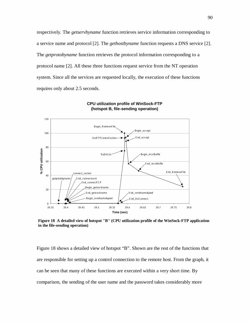
90

respectively. The getservbyname function retrieves service information corresponding to

a service name and protocol [2]. The gethostbyname function requests a DNS service [2].

The getprotobyname function retrieves the protocol information corresponding to a

protocol name [2]. All these three functions request service from the NT operation

system. Since all the services are requested locally, the execution of these functions

requires only about 2.5 seconds.

CPU utilization profile of WinSock-FTP(hotspot B, file-sending operation)

0

20

40

60

80

100

120

39.35 39.4 39.45 39.5 39.55 39.6 39.65 39.7 39.75 39.8

Time (sec)

%C

PU

uti

lizat

ion

getprotobyname

connect_socket

End_connectsock

End_connectTCP

Begin_getsockname

End_getsockname

Begin_sendname&pwd

End_sendname&pwd

End_DoConnect

DoDirList

Begin_RetrieveFile

GetFTPListenSocket

Begin_accept

End_accept

Begin_recvthefile

End_recvthefile

End_RetrieveFile

Figure 18 shows a detailed view of hotspot “B”. Shown are the rest of the functions that

are responsible for setting up a control connection to the remote host. From the graph, it

can be seen that many of these functions are executed within a very short time. By

comparison, the sending of the user name and the password takes considerably more

Figure 18 A detailed view of hotspot "B" (CPU utilization profile of the WinSock-FTP applicationin the file-sending operation)

91

time, about 0.17 second. This can be explained by the need to transmit authentication

information through the newly-established control connection to the remote host. A total

of approximately 0.2 second is spent by the rest of the functions for setting up a control

connection. In terms of CPU usage, these functions consume next to nothing as they

require no service from the NT operating system. After the control connection was set up,

a CPU utilization spur, which is short by definition, occurs when the function, DoDirList,

is called. Since the WinSock-FTP is a graphical-user-interface application, it

automatically displays the list of remote files for user selection once the control

connection has been established. In order to display the list of remote files, the WinSock-

FTP application needs to establish a data connection to the remote host and retrieve the

name list of the remote files to the local computer. These operations require a lot of data

transfer and processing in a short period of time. Therefore, they cause a sudden and

significant increase in CPU utilization. As shown in the graph, the CPU usage jumped to

100 percent during the retrieval of the name list of the remote files. After this CPU-

intensive operation has finished, the CPU usage gradually declines back to the original

level.

.

92

CPU utilization profile of WinSock-FTP(hotspot C, file-sending operation)

0

20

40

60

80

100

120

43.1 43.15 43.2 43.25 43.3 43.35 43.4 43.45 43.5

Time (sec)

%C

PU

uti

lizat

ion

OnCmdLocalToRemote

Begin_SendFile

GetFTPListenSocket

Begin_accept

End_acceptBegin_sendthefile

End_sendthefile

End_SendFile

DoDirList

Begin_RetrieveFile

GetFTPListenSocket

Begin_accept

End_acceptBegin_recvthefile

End_recvthefile

End_RetrieveFile

Figure 19 shows the detailed view of hotspot “C”. First of all, it shows that a small

number of functions are called by the WinSock-FTP application to set up a data

connection for the purpose of file sending. From the graph, we know that the time of

establishing the data connection is fairly short, which is about 0.01 second. Also, it takes

about 0.15 second for sending a file of 100 kilobytes. The relationship between the size

of the sending files and their corresponding latency is presented later in this chapter. The

sending and receiving of a file are two major operations that consume a large amount of

CPU time. There is a large amount of data copying (data-touching operation) [11]

involved during this process. When only a small file is sent, as this case, the sending

operation only occupies about 5 percent of the CPU time. After the operation comes

Figure 19 A detailed view of hotspot "C" (CPU utilization profile of WinSock-FTP application inthe file-sending operation)

93

another huge spur. The pattern of this spur is very similar to the previous one. This spur

comes about as a result of another file name lookup operation. Since the name of the file

to be sent might not exist in the existing remote file list, the WinSock-FTP application

may need to retrieve the name list of the remote files from the remote computer once

again to update the local name list of the remote files.

8.1.2 CPU Utilization Profile of the File-Receiving Operation

The following diagrams illustrate the relationship of both latency and throughput with

respect to the size of the file being received in the file-receiving operation.

CPU utilization profile of WinSock-FTP(Retrieving a 100kb file)

0

10

20

30

40

50

60

70

80

90

100

0 5 10 15 20 25 30 35 40 45 50

Time (sec)

%C

PU

uti

lizat

ion

Time spent by user onchoosing the remote hostto connect to

Time spent by the FTP client on obtaining DNS

Time spent by user onchoosing the remote fileto retrieve

Time spent by useron quitting the FTP

A

B

C

Begin_WinMain

End_WinMain

Figure 20 Overall CPU utilization profile of the WinSock-FTP application in the file-receivingoperation

94

Figure 20 shows the CPU usage of the WinSock-FTP application with respect to time

during the entire process of the file-receiving operation. As we expected, the graph looks

very similar to the graph of the file-sending operation, except it shows the presence of a

single huge spur only. This difference is due to the fact that the WinSock-FTP application

only needs to retrieve the name list of the remote files for user selection once only, when

it first connects to the remote host. After retrieving the files from the remote host, it is not

necessary for the application to retrieve the name list of the remote files again, as in the

case of the file-sending operation, since the list of remote files still remains the same.

There are again four periods of waiting during the file-receiving operation. Referring to

the description of the overall CPU utilization of the file-sending operation, the length of

waiting period (1), (3) and (4) vary with the response of the user. By the contrast, it still

takes about 36 seconds, which is same as the waiting time of the file-sending operation,

to perform DNS. The following shows the detailed view of the three areas.

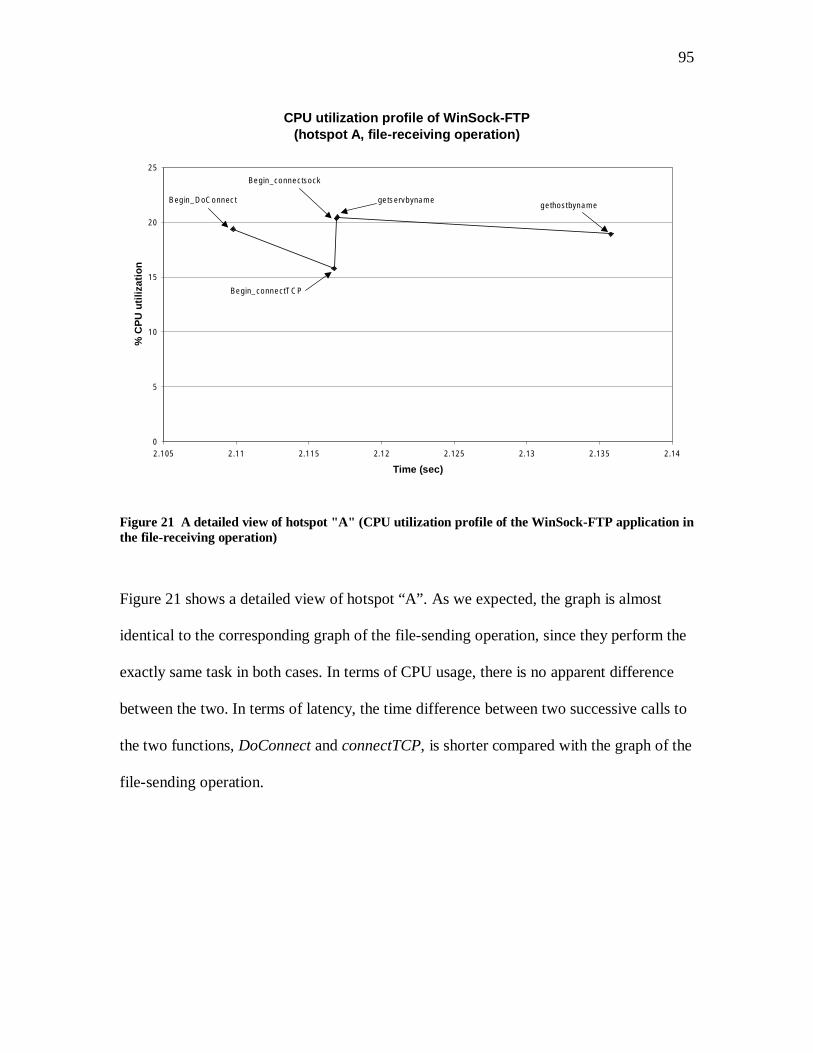
95

CPU utilization profile of WinSock-FTP(hotspot A, file-receiving operation)

0

5

10

15

20

25

2.105 2.11 2.115 2.12 2.125 2.13 2.135 2.14

Time (sec)

%C

PU

uti

lizat

ion

Begin_DoConnect

Begin_connectTCP

Begin_connectsock

getservbynamegethostbyname

Figure 21 A detailed view of hotspot "A" (CPU utilization profile of the WinSock-FTP application inthe file-receiving operation)

Figure 21 shows a detailed view of hotspot “A”. As we expected, the graph is almost

identical to the corresponding graph of the file-sending operation, since they perform the

exactly same task in both cases. In terms of CPU usage, there is no apparent difference

between the two. In terms of latency, the time difference between two successive calls to

the two functions, DoConnect and connectTCP, is shorter compared with the graph of the

file-sending operation.

96

CPU utilization profile of WinSock-FTP(hotspot B, file-receiving operation)

0

10

20

30

40

50

60

70

80

90

100

39 39.2 39.4 39.6 39.8 40 40.2 40.4

Time (sec)

%C

PU

uti

lizat

ion

getprotobyname

connect_socket

End_connectsock

End_connectTCP

Begin_getsockname

End_getsockname

Begin_sendname&pwd

End_sendname&pwd

End_DoConnect

DoDirList

Begin_RetrieveFile

GetFTPListenSocket

Begin_accept End_accept

Begin_recvthefile

End_recvthefile

End_RetrieveFile

Figure 22 A detailed view of hotspot "B" (CPU utilization profile of the WinSock-FTP application inthe file-receiving operation)

Figure 22 shows the detailed view of hotspot “B”. Generally speaking, it is similar to the

corresponding graph of the file-sending operation. However, they are different in a

number of places. First of all, the execution time between the two instrumentation points,

End_getsockname and Begin_sendname&pwd, is longer. In addition, the CPU usage of

retrieving the name list of the remote files is only 90 percent compared to 100 percent of

CPU usage for the file-sending operation. Both the file-sending and the file-receiving

operations initiate the same call to establish the control connection and retrieve the name

list of the remote files; therefore, we believe that the difference is due to the averaging of

total number of data.

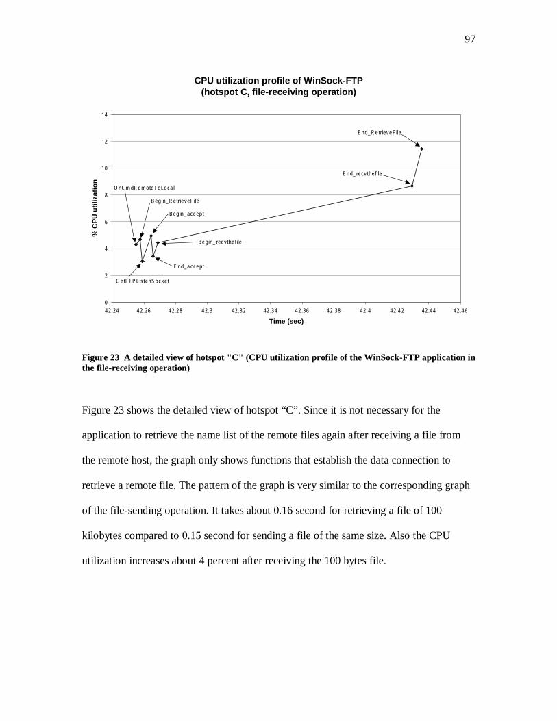
97

CPU utilization profile of WinSock-FTP(hotspot C, file-receiving operation)

0

2

4

6

8

10

12

14

42.24 42.26 42.28 42.3 42.32 42.34 42.36 42.38 42.4 42.42 42.44 42.46

Time (sec)

%C

PU

uti

lizat

ion

OnCmdRemoteToLocal

Begin_RetrieveFile

GetFTPListenSocket

Begin_accept

End_accept

Begin_recvthefile

End_recvthefile

End_RetrieveFile

Figure 23 A detailed view of hotspot "C" (CPU utilization profile of the WinSock-FTP application inthe file-receiving operation)

Figure 23 shows the detailed view of hotspot “C”. Since it is not necessary for the

application to retrieve the name list of the remote files again after receiving a file from

the remote host, the graph only shows functions that establish the data connection to

retrieve a remote file. The pattern of the graph is very similar to the corresponding graph

of the file-sending operation. It takes about 0.16 second for retrieving a file of 100

kilobytes compared to 0.15 second for sending a file of the same size. Also the CPU

utilization increases about 4 percent after receiving the 100 bytes file.

98

8.2 CPU Utilization Profile of the NcFTP Application

8.2.1 CPU Utilization Profile of the File-Sending Operation


respect to the size of file being sent in the file-sending operation.

CPU utilization profile of NcFTP(Sending a 4000kb file)

0

10

20

30

40

50

60

70

80

90

100

0 1 2 3 4 5 6 7 8 9 10

Time (sec)

%C

PU

Uti

lizat

ion

Time spent by user on typing forconnecting to remote host

Time spent by user on typing forsending a local file

Time spent onfile transfer

Time spent by user on typingQuit command

B

C

D

A

CloseDataConnection w32_closesocket

EndTransfe

Figure 24 Overall CPU utilization profile of the NcFTP application in the file-sending operation

Figure 24 shows the CPU usage of the NcFTP application with respect to time during the

entire process of the file-sending operation. As indicated in the graph, most of the

functions along the execution path of the file-sending operation are only executed in a

small portion of the entire period. A close-up view of these functions and a detailed

99

discussion are presented in this section later. Like the WinSock-FTP application, the

NcFTP application spends most of its time in waiting for the user input or performing file

transfer during the file-sending operation. From our results, it shows that the NcFTP

application spends most of its time in the following:

(1) It spends about 2.5 seconds to wait for the user input to connect to the remote host

(2) It spends another 3 seconds to wait for the user input to select the file to be sent

(3) It then spends about 1 second to send a 4000 kilobytes file

(4) Finally, it spends about 2 seconds to wait for the user input to quit the application

In terms of CPU usage, there are a few operations that cause a significant amount of

consumption of CPU time. They are listed as follows:

(1) Establishes a control connection to the remote host

(2) Sends a specified local file to the remote host

(3) Deallocates the resources of the application and exits.

100

CPU utilization profile of NcFTP(hotspot A, file-sending operation)

0

0.5

1

1.5

2

2.5

3

3.5

4

4.5

0 0.01 0.02 0.03 0.04 0.05 0.06

Time (sec)

%C

PU

uti

lizat

ion

Begin_Main

Init

w32_setsockopt

GetOurHostNam

GetHostEntry

InitDefaultFTPPortUserLoggedIn

getwd

RunStartUpScrip

GetOpenOption

Figure 25 A detailed view of hotspot "A" (CPU utilization profile of the NcFTP application in thefile-sending operation)

Figure 25 shows the detailed view of hotspot “A”. All the functions shown in this

diagram are automatically executed when the NcFTP application starts. These functions

basically perform the initialization procedure for the application such as getting the name

of local host, and pursing anonymous user login and password, etc. From the graph, it

shows that these functions consume very low percentage of CPU time, which is around 3

to 4 percent. It is because these functions only query information from the local

computer. This type of operation should be very quick and simple; therefore, the result

matches our expectation.

101

CPU utilization profile of NcFTP(hotspot B, file-sending operation)

0

2

4

6

8

10

12

14

2.614 2.616 2.618 2.62 2.622 2.624 2.626 2.628 2.63 2.632 2.634 2.636

Time (sec)

%C

PU

uti

lizat

ion

ExecCommandLine

DoClose

CloseControlConnection

CloseDataConnection

GetOpenOptionsOpenControlConnection

GetHostEntry

w32_socket

w32_connect

w32_getsockname

w32_setsockopt

Close_OpenControlConnection

Figure 26 A detailed view of hotspot "B" (CPU utilization profile of the NcFTP application in thefile-sending operation)

Figure 26 shows the detailed view of hotspot “B”. First of all, the application interprets

the user command to determine what operation requested by the user. Once it determines

that the user requests to set up a control connection to the remote host, it starts the

corresponding procedure. The figure shows all the functions that are responsible for

establishing a control connection to the remote host. As shown, the average CPU usage of

these functions is about 6 percent higher than the average CPU usage of the initialization

procedure. From the graph, we also realize the CPU usage tends to increase gradually

from 6 to 13 percent during the process of setting up the control connection. Since this

sequence of functions requests name look-up service and minor data transfer from the

operation system, it is obvious that the CPU usage increases. Once the connection is set

102

up, the CPU usage falls back to about 3 percent. This phenomenon further ensures our

assumption. Therefore, the results we got are consistent with our expectation.

CPU utilization profile of NcFTP(hotspot C, file-sending operation)

0

0.5

1

1.5

2

2.5

3

3.5

5.618 5.62 5.622 5.624 5.626 5.628 5.63 5.632 5.634 5.636

Time (sec)

%C

PU

uti

lizat

ion

ExecCommandLine

PutCmd

GetLocalSendFileName

OpenLocalSendFile

BinaryPut

Begin_OpenDataConnection

w32_socket

w32_bind

w32_getsockname

w32_listen

w32_setsockopt

End_OpenDataConnection

AcceptDataConnection

w32_accept

w32_closesocket

StartTransferStdFileSend

Figure 27 A detailed view of hotspot "C" (CPU utilization profile of the NcFTP application in thefile-sending operation)

Figure 27 shows the detailed view of hotspot “C”. First of all, it interprets the user

command to determine that the user requests to send a local file to the remote host. It

starts to open the local file for read. Then, it sets up a data connection to the remote host.

Once the data connection has established, it starts to send the file. From our result, it

indicates that these procedures only contribute an average CPU usage of 2 to 3 percent.

Then, we notice that there is a huge increase of CPU usage during the process of the file

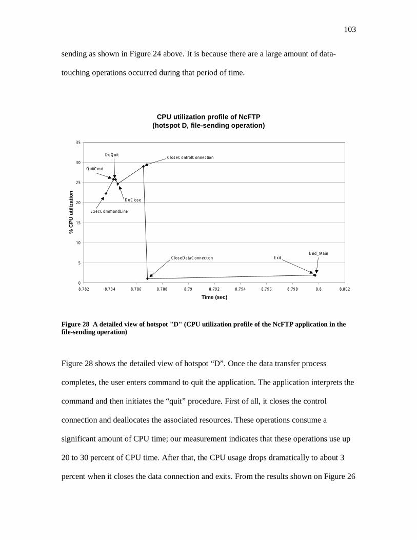
103

sending as shown in Figure 24 above. It is because there are a large amount of data-

touching operations occurred during that period of time.

CPU utilization profile of NcFTP(hotspot D, file-sending operation)

0

5

10

15

20

25

30

35

8.782 8.784 8.786 8.788 8.79 8.792 8.794 8.796 8.798 8.8 8.802

Time (sec)

%C

PU

uti

lizat

ion

ExecCommandLine

QuitCmd

DoQuit

DoClose


CloseDataConnection ExitEnd_Main

Figure 28 A detailed view of hotspot "D" (CPU utilization profile of the NcFTP application in thefile-sending operation)

Figure 28 shows the detailed view of hotspot “D”. Once the data transfer process

completes, the user enters command to quit the application. The application interprets the

command and then initiates the “quit” procedure. First of all, it closes the control

connection and deallocates the associated resources. These operations consume a

significant amount of CPU time; our measurement indicates that these operations use up

20 to 30 percent of CPU time. After that, the CPU usage drops dramatically to about 3

percent when it closes the data connection and exits. From the results shown on Figure 26

104

and Figure 28, it implies that opening or closing a control connection depletes much more

CPU time than opening or closing a data connection.

8.2.2 CPU Utilization Profile of the File-Receiving Operation


respect to the size of file being received in the file-receiving operation.

CPU utilization profile of NcFTP(Retrieving a 4000kb file)

0

10

20

30

40

50

60

70

80

0 2 4 6 8 10 12 14 16Time (sec)

%C

PU

Uti

lizat

ion

Time spent by user on typingfor connecting to remote host

Time spent by user on typing forretrieving a remote file Time spent on file transfer

Time spent by useron typing Quitcommand

A

B

C

D

E

CloseDataConnection

w32_closesocket

EndTransfer

Figure 29 Overall CPU utilization profile of the NcFTP application in the file-receiving operation

Figure 29 shows the CPU usage of the NcFTP application with respect to time during the

entire process of the file-receiving operation. When we compare the result with those of

the file-sending operation, we realize that they are almost the same. The major

105

differences are (1) the CPU usage at the end of file transfer process is lower for the file-

receiving operation, which is about 70 to 75 percent, and (2) the CPU usage of the “Quit”

procedure is higher, which is about 55 percent.

CPU utilization profile of NcFTP(hotspot A, file-receiving operation)

3.45

3.5

3.55

3.6

3.65

3.7

3.75

3.8

3.85

3.9

0 0.01 0.02 0.03 0.04 0.05 0.06

Time (sec)

%C

PU

uti

lizat

ion

Begin_Main

Init

w32_setsockopt

GetOurHostName

GetHostEntry

InitDefaultFTPPort

UserLoggedIn

getwd

RunStartupScript

GetOpenOptions

Figure 30 A detailed view of hotspot "A" (CPU utilization profile of the NcFTP application in thefile receiving operation)

Figure 30 shows the detailed view of hotspot “A”. It shows the initialization functions of

the file-receiving operation. All of these functions consume CPU time in the range of 3.4

to 3.9 percent. The result here is consistent with the result of the file-sending operation

previously.

106

CPU utilization profile of NcFTP(hotspot B, file-receiving operation)

0

2

4

6

8

10

12

14

16

3.275 3.28 3.285 3.29 3.295 3.3

Time (sec)

%C

PU

uti

lizat

ion

ExecCommandLine

DoClose


CloseDataConnection

GetOpenOptions

OpenControlConnection

GetHostEntry

w32_socket

w32_connect

w32_getsockname

w32_setsockopt

Close_OpenControlConnection

Figure 31 A detailed view of hotspot "B" (CPU utilization profile of the NcFTP application in thefile-receiving operation)

Figure 31 shows the detailed view of hotspot “B”. As we expect, the CPU consumption

for establishing a control connection is higher than the initialization procedure. From our

result, it shows that the CPU consumption of these functions falls in the range of 6 to 14

percent. In addition, the result here matches the result of the file-sending operation we

presented previously.

107

CPU utilization profile of NcFTP(hotspot C, file-receiving operation)

0

0.5

1

1.5

2

2.5

3

3.5

4

7.149 7.15 7.151 7.152 7.153 7.154 7.155 7.156 7.157

Time (sec)

%C

PU

uti

lizat

ion

ExecCommandLine

GetCmdDoGet

CloseDataConnection


w32_socket

w32_bind

w32_getsockname

w32_listen

w32_setsockopt

End_OpenDataConnection


w32_accept

w32_closesocket

StartTransfer

CloseDataConnection

w32_closesocket

EndTransfer

Figure 32 A detailed view of hotspot "C" (CPU utilization profile of the NcFTP application in thefile-receiving operation)

Figure 32 shows the detailed view of hotspot “C”. It shows one of the major differences

between the file-sending and file-receiving operations in the NcFTP application. This

sequence of functions is only executed when the file-receiving operation is performed.

The purpose is to find out the date and the size of the file before it is retrieved. This

information allows the application to determine whether the local computer has already

had the most updated version of the file. If not, the application will retrieve the remote

file; otherwise, it leaves the same file alone by default. Such a feature is designed for

efficiency but is specific to the NcFTP application. From the graph, it shows this

mechanism only uses up about 2 to 4 percent of CPU time, which is about the same CPU

usage for setting up a data connection.

108

CPU utilization profile of NcFTP(hotspot D, file-receiving operation)

0

1

2

3

4

5

6

7

8

9

7.252 7.254 7.256 7.258 7.26 7.262 7.264

Time (sec)

%C

PU

uti

lizat

ion

BinaryGet

CloseDataConnection


w32_socket

w32_bind

w32_getsockname

w32_listen

w32_setsockoptEnd_OpenDataConnection


w32_accept

w32_closesocket

StartTransfer

StdFileReceive

Figure 33 A detailed view of hotspot "D" (CPU utilization profile of the NcFTP application in thefile-receiving operation)

Figure 33 shows the detailed view of hotspot “D”. This figure shows the functions that

set up a data connection for retrieving the file. Their CPU usage is in the range of 4 to 8

percent. It is about 3 percent higher than those of the file-sending operation. The higher

CPU processing time is due to the fact that the implementation of the receiving side is

more complex than that of the sending side in the Windows NT operation system. It

involves buffering for sequencing the received packets before the data is sent up to the

application.

109

CPU utilization profile of NcFTP(hotspot E, file-receiving operation)

0

10

20

30

40

50

60

70

14.226 14.228 14.23 14.232 14.234 14.236 14.238 14.24 14.242 14.244 14.246

Time (sec)

%C

PU

uti

lizat

ion

ExecCommandLine QuitCmd

DoQuit

DoClose


CloseDataConnection

Exit

End_Main

Figure 34 A detailed view of hotspot "E" (CPU utilization profile of the NcFTP application in thefile-receiving operation)

Figure 34 shows the detailed view of hotspot “E”. This diagram shows the CPU

utilization of the “Quit” procedure of the file-receiving operation. It indicates the “Quit”

procedure takes about 55 percent of CPU time to deallocate the resources. It is about 25

percent higher than the same procedure executed by the file-sending operation. Also, we

notice that the CPU usage jumps to 55 percent when the application is closed.

8.3 Latency and Throughput of the WinSock-FTP Application

8.3.1 Latency and Throughput of the File-Sending Operation


respect to the size of file being sent in the file-sending operation.

110

Relationship between number of bytes sent and time taken of a GUI FTP application duringfile transfer (small scale)

0

1000

2000

3000

4000

5000

6000

7000

0 0.5 1 1.5 2 2.5 3 3.5 4 4.5

Number of bytes sent (kilobyte)

Tim

eta

ken

bet

wee

nst

art

and

retu

rno

fS

end

fun

ctio

n(m

icro

seco

nd

)

Figure 35 The latency of the WinSock-FTP application for sending file in the range of 100 to 4000bytes

Figure 35 shows the relationship between the time duration of sending a file and the size

of the file being sent in the range of 100 to 4000 bytes. As we expect, the trend of the

graph indicates that the latency increases as the size of file increases. However, the

latency increases in a stepwise format as the file size increases. Each step spans about

500 bytes. In other words, the latency only increases slightly as the file size increases up

to 500 bytes. Then the latency increases significantly when the file size exceeds 500

bytes. After that, the latency increases slightly again until the file size reaches 1000 bytes.

This pattern repeats itself for every 500 bytes increment. Such a circumstance can be

explained as follows. When a network application sends data to or received data from the

network, the information is exchanged in the form of segment through the transport layer

111

protocol, TCP. A segment is composed of a fixed 20-byte header followed by zero or

more data bytes. The size of segment is determined by TCP but is restricted by two

factors. First, each segment, including the TCP header, must fit in the 65,535-byte IP

payload. Second, each network has a maximum transfer unit (MTU), and each segment

must fit in the MTU. In this experiment, we run our test on two NT workstations that are

connected by 100 Mbps Ethernet. The maximum transmission unit (MTU) of Ethernet is

1500 bytes. It means that the upper bound on segment size is 1500 bytes in this case. If

the data size is less than 1500 bytes, it can all fit in one segment and passes through the

network without being fragmented. Therefore, there is no apparent delay for the increase

of data size. However, if the data size is more than 1500 bytes, the data need to be

fragmented to fit in the 1500-byte segment and also requires at least another segment to

transmit the rest of data. Each time the data is fragmented to fit into the smaller segment

size, it introduces a significant amount of delay. Due to such a unique pattern shown in

our graph, we believe that it somehow relates to the fragmentation mechanism in the

network layer of the TCP/IP stack.

112

Relationship between number of bytes sent and time taken of a GUI FTP application duringfile transfer (large scale)

y = 1286.7x + 7777.4

0

200000

400000

600000

800000

1000000

1200000

1400000

0 200 400 600 800 1000 1200


Tim

eta

ken

bet

wee

nst

art

and

retu

rno

fS

end

fun

ctio

n(m

icro

sec)

Figure 36 The latency of the WinSock-FTP application for sending file in the range of 100 to 1000kilobytes


of the file being sent in the range of 100 to 1000 kilobytes. The purpose of this

measurement is to find out the trend of latency as the size of file increases in a large

scale. By doing that, we hope we can predict the change of latency when the file size

becomes infinitely large. From the graph, it indicates the latency increases linearly as the

size of file increases. It roughly introduces an additional latency of 0.13 second for each

increase of file size of 100 kilobytes.

113

Relationship between transfer file size and throughput of a GUI FTP application(small scale)

0

100

200

300

400

500

600

700

0 0.5 1 1.5 2 2.5 3 3.5 4 4.5


Th

rou

gh

pu

t(k

ilob

yte/

sec)

Figure 37 The throughput of the WinSock-FTP application for sending file in the range of 100 to4000 bytes

Figure 37 shows the relationship between throughput and the size of file being sent in the

range of 100 to 4000 bytes. The throughput value is calculated by dividing the size of file

with latency shown in the above two figures. Therefore, the see-saw pattern of the

throughput curve is due to the step-wise pattern of the latency curve. From the graph, it

indicates that the throughput increases as the size of file increases. However, the rate of

increase decreases as the size of file increases. Such a trend suggests to us that the

throughput rate will level off at a certain size of the file. In other word, after passing that

point (file size), further increase in the file size will not increase the throughput.

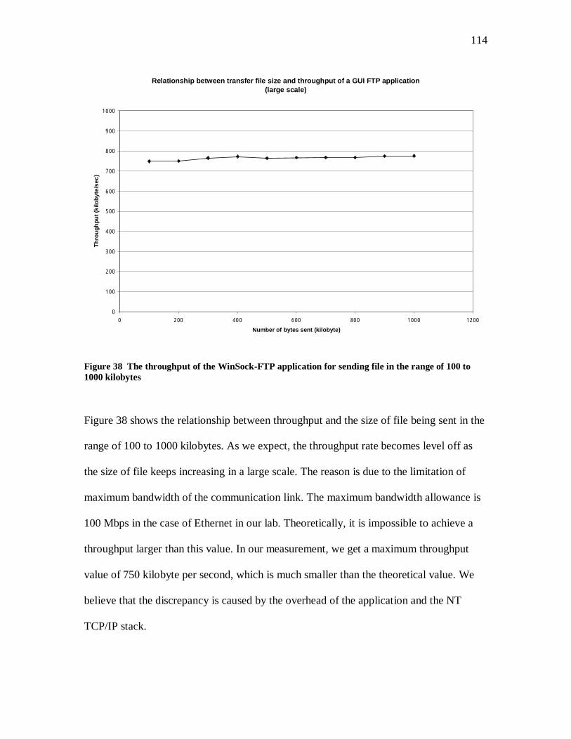
114

Relationship between transfer file size and throughput of a GUI FTP application(large scale)

0

100

200

300

400

500

600

700

800

900

1000

0 200 400 600 800 1000 1200


Th

rou

gh

pu

t(k

ilob

yte/

sec)

Figure 38 The throughput of the WinSock-FTP application for sending file in the range of 100 to1000 kilobytes

Figure 38 shows the relationship between throughput and the size of file being sent in the

range of 100 to 1000 kilobytes. As we expect, the throughput rate becomes level off as

the size of file keeps increasing in a large scale. The reason is due to the limitation of

maximum bandwidth of the communication link. The maximum bandwidth allowance is

100 Mbps in the case of Ethernet in our lab. Theoretically, it is impossible to achieve a

throughput larger than this value. In our measurement, we get a maximum throughput

value of 750 kilobyte per second, which is much smaller than the theoretical value. We

believe that the discrepancy is caused by the overhead of the application and the NT

TCP/IP stack.

115

8.4.2 Latency and Throughput of the Receiving Operation


respect to the size of file being received in the file-receiving operation.

Relationship between number of bytes received and time taken of a GUI FTP applicationduring file transfer (small scale)

0

20000

40000

60000

80000

100000

120000

140000

160000

180000

0 0.5 1 1.5 2 2.5 3 3.5 4 4.5

Number of bytes received (byte)

Tim

eta

ken

bet

wee

nst

art

and

retu

rno

fR

ecei

ved

fun

ctio

n(m

icro

seco

nd

)

Figure 39 The latency of the WinSock-FTP application for receiving file in the range of 100 to 4000bytes

Figure 39 shows the relationship between the time duration (latency) of receiving a file

and the size of the file being received in the range of 100 to 4000 bytes. As we have seen,

the latency curve of receiving a file is quite different from that of sending a file. From the

graph, it indicates that the latency is approximately 150,000 microseconds (0.15 second)

for the file size between 100 to 1400 bytes. Then the latency drops dramatically to around

4,000 microseconds for the file size between 1500 to 2900 bytes, which is very close to

116

the sending latency for the same file size range. Then the latency jumps to 150,000

microseconds again for the file size between 3000 to 3600 bytes. After that, it drops back

to about 5,000 microseconds for the file size between 3700 to 4000 bytes. This latency

pattern is totally out of our expectation. At the beginning, we thought we have got an

incorrect measurement. Therefore, we repeated our experiments several times to verify

our results. Consequently, the results are very consistent and repeatable. Also, we verified

our instrumentation method is exactly the same as we got our latency result for file

sending.

Relationship between number of bytes received and time taken of a GUI FTP applicationduring file transfer (large scale)

y = 1281.3x - 74807

0

500000

1000000

1500000

2000000

2500000

3000000

0 500 1000 1500 2000 2500

Number of bytes received (kilobyte)

Tim

eta

ken

bet

wee

nst

art

and

retu

rno

fR

ecei

vefu

nct

ion

(mic

rose

con

d)

Figure 40 The latency of the WinSock-FTP application for receiving file in the range of 1000 to 2000kilobytes

117


of the file being received in the range of 100 to 2000 kilobytes. When we look at the

relationship of latency and the size of the receiving file in a bigger picture, our result

indicates that the curve grows linearly as the result shown in Figure YYY for the file

sending. Comparing both results, it seems that the latency curves of both the file-sending

and the file-receiving have the same growing rate with respect to the size of the file.

However, the time of the file receiving is always 15,000 microseconds less than the time

of the file sending for each corresponding file size. We believe that such a difference is

caused by the different implementation of the sending and the receiving functions. In the

WinSock-FTP application, the function SendMass is responsible for sending a local file

and the function ReadMass is responsible for receiving a remote file. However,

SendMass in terms calls another function SendStr to perform the actual file sending;

whereas, ReadMass performs the actual file receiving itself. Each time the SendStr

function is called, an extra time delay (overhead) is introduced to our measurement.

Therefore, our result shows this constant difference.

118

Relationship between transfer file size and throughput of a GUI FTP application(small scale)

0

200

400

600

800

1000

1200

1400

0 0.5 1 1.5 2 2.5 3 3.5 4 4.5


Th

rou

gh

pu

t(k

ilob

yte/

sec)

Figure 41 The throughput of the WinSock-FTP application for receiving file in the range of 100 to4000 bytes

Figure 41 shows the relationship between throughput and the size of file being received

in the range of 100 to 4000 bytes. As mentioned earlier, the throughput value is

calculated by dividing the file size with its corresponding latency of file transfer. It is

expected that we have a sort of graph which looks like the reciprocal of the latency curve.

From the graph, it indicates that there is only extremely small throughput for the file size

in the range of 100 to 1400 bytes and 3000 to 3600 bytes. Conversely, there is a

reasonable amount of throughput when the receiving file has a size in a range of 1500 to

2900 bytes and 3700 to 4000 bytes. Also, we can see that the throughput increases as the

file size increases in the specified range.

119

Relationship between transfer file size and throughput of a GUI FTP application(large scale)

0

200

400

600

800

1000

1200

0 500 1000 1500 2000 2500


Th

rou

gh

pu

t(k

ilob

yte/

sec)

Figure 42 The throughput of the WinSock-FTP application for receiving file in the range of 100 to2000 kilobytes

Figure 42 shows the relationship between throughput and the size of file being received

in the range of 100 to 2000 kilobytes. From the graph, it indicates the throughput rate is

about 1100 kilobytes per second for receiving a file of 100 kilobyte. However, as the file

size is getting bigger, the throughput rate gradually declines. Finally, the throughput rate

levels off at the throughput rate of 800 kilobytes per second. Compared with the ultimate

throughput rate of 750 kilobytes per second for the file sending, the file receiving seems

to have a higher ultimate throughput. However, we believe such a small discrepancy is

due to our limited sample size. If the sample size were bigger, the difference should be

insignificant. In other words, the ultimate throughput rate for both the file sending and the

file receiving should be the same. Furthermore, since the throughput decreases at the

120

beginning and levels off eventually, it suggests to us that there exists an optimum file size

in the range of 4000 bytes to 100 kilobytes, where yields the maximum throughput.

8.4 Latency and Throughput of the NcFTP Application

8.4.1 Latency and Throughput of the File-Sending Operation


respect to the size of the file being sent in the file-sending operation.

Relationship between number of bytes sent and time taken of NcFTP application during filetransfer (small scale)

0

500

1000

1500

2000

2500

3000

3500

4000

4500

5000

0 0.5 1 1.5 2 2.5 3 3.5 4 4.5


Tim

eta

ken

bet

wee

nb

egin

nin

gan

den

do

ffi

letr

ansf

er(m

icro

seco

nd

)

Figure 43 The latency of the NcFTP application for sending file in the range of 100 to 4000 bytes

Figure 43 shows the relationship between the time duration (latency) of sending a file and

the size of the file being sent in the range of 100 to 4000 bytes. From the graph, it

121

illustrates the latency increases slightly as the size of the file increases. Compared with

the result of the WinSock-FTP, the increase rate of latency of the NcFTP application is

much less. However, the latency curve does not show the same type of step-wise pattern

as the WinSock-FTP application does. It is kind of random with a tendency of slight

increase.

Relationship between number of bytes sent and time taken of NcFTP application during filetransfer (large scale)

y = 184.42x - 9880.6

0

100000

200000

300000

400000

500000

600000

700000

800000

0 500 1000 1500 2000 2500 3000 3500 4000 4500


Tim

eta

ken

bet

wee

nb

egin

nin

gan

den

do

ffi

letr

ansf

er(m

icro

seco

nd

)

Figure 44 The latency of the NcFTP application for sending file in the range of 100 to 4000 kilobytes


of the file being sent in the range of 100 to 4000 kilobytes. It is expected that the latency

curve will grow linearly as the file size increases in a large scale. However, as mentioned

earlier, the increase rate of latency of the NcFTP application is much less than that of the

WinSock-FTP application. According to Figure 37, the WinSock-FTP application

122

introduces 1287 microseconds of latency for each additional kilobyte of file being sent in

the average. Conversely, the NcFTP application only introduces 184 microseconds of

latency, which is about 7 times less.

Relationship between sending file size and throughput of NcFTP application(small scale)

0

200

400

600

800

1000

1200

0 0.5 1 1.5 2 2.5 3 3.5 4 4.5


Th

rou

gh

pu

t(k

ilob

yte/

sec)

Figure 45 The throughput of the NcFTP application for sending file in the range of 100 to 4000 bytes

Figure 45 shows the relationship between throughput and the size of the file being sent in

the range of 100 to 4000 bytes. From the graph, it shows that the throughput increases in

a fairly linear fashion throughout the entire range of file size. Compared with the

WinSock-FTP application, the NcFTP application has a higher throughput for sending the

file.

123

Relationship between sending file size and throughput of NcFTP application(large scale)

0

1000

2000

3000

4000

5000

6000

7000

0 500 1000 1500 2000 2500 3000 3500 4000 4500


Th

rou

gh

pu

t(k

ilob

yte/

sec)

Figure 46 The throughput of the NcFTP application for sending file in the range of 100 to 4000kilobytes

Figure 46 shows the relationship between throughput and the size of the file being sent in

the range of 100 to 4000 kilobytes. It indicates that the ultimate throughput rate of the file

sending of the NcFTP application is about 5500 kilobytes per second. Conversely, the

maximum throughput of the WinSock-FTP application is only 750 kilobytes per second.

Therefore, the file-sending throughput of the NcFTP application is about 7.3 times

higher.

124

8.4.2 Latency and Throughput of the Receiving Operation

Relationship between number of bytes received and time taken of NcFTP application duringfile transfer (small scale)

0

50000

100000

150000

200000

250000

0 0.5 1 1.5 2 2.5 3 3.5 4 4.5


Tim

eta

ken

bet

wee

nb

egin

nin

gan

den

do

ffi

letr

ansf

er(m

icro

seco

nd

)

Figure 47 The latency of the NcFTP application for receiving file in the range of 100 to 4000 bytes

Figure 47 shows the relationship between the time duration (latency) of receiving a file

and the size of the file being received in the range of 100 to 4000 bytes. From the graph,

it indicates that we have the same unusual pattern as we measure the latency of the file

receiving introduced by the WinSock-FTP application. Such a common pattern suggests

that the cause come from the NT operating system rather than either one of the specific

FTP implementations or instrumentation and measurement errors. Finally, we determine

that the cause is due to the late return of the receiving socket function, recv for the

WinSock-FTP application and read for the NcFTP application. Usually, this function is

located inside an infinite loop that continuously reads data from the data connection until

125

the end of data stream. Once all the data has been read, the operating system returns a

value of 0 or less as a delimiter to indicate the end of data. The function constantly

checks for its return value to look for the delimiter. Once found, it exits the infinite loop.

However, we find out that the receiving function takes a long time to return for certain

file sizes when the end of data stream has been reached. It seems that there are some

algorithms inside the NT operating system to determine whether it should return

immediately if no more data is coming.

Relationship between number of bytes received and time taken of NcFTP application duringfile transfer (large scale)

y = 1546.1x - 26169

0

1000000

2000000

3000000

4000000

5000000

6000000

7000000

0 500 1000 1500 2000 2500 3000 3500 4000 4500


Tim

eta

ken

bet

wee

nb

egin

nin

gan

den

do

ffi

letr

ansf

er(m

icro

seco

nd

)

Figure 48 The latency of the NcFTP application for receiving file in the range of 100 to 4000kilobytes

Figure 48 shows the relationship between the time duration of receiving a file and the

size of the file being received in the range of 100 to 4000 kilobytes. When we look at the

126

change in latency of the receiving function with respect to different size of files in a large

scale, there is a linear relation between them. But the increase rate of latency for the

NcFTP application (1546 microseconds increase in latency per additional 100 kilobytes)

is a little bit higher than that for the WinSock-FTP application (1281 microseconds

increase in latency per additional 100 kilobytes).

Relationship between receiving file size and throughput of NcFTP application (small scale)

0

100

200

300

400

500

600

700

800

900

0 0.5 1 1.5 2 2.5 3 3.5 4 4.5


Th

rou

gh

pu

t(k

ilob

yte/

sec)

Figure 49 The throughput of the NcFTP application for receiving file in the range of 100 to 4000bytes

Figure 49 shows the relationship between throughput and the size of the file being

received in the range of 100 to 4000 bytes. As we expect, there is very little throughput

for the file size in the range of 100 to 1400 bytes and 3000 to 3600 bytes. And there is an

127

increasing throughput for the file size in the range of 1500 to 2900 bytes and 3700 to

4000 bytes.

Relationship between receiving file size and throughput of NcFTP application(large scale)

0

100

200

300

400

500

600

700

800

900

0 500 1000 1500 2000 2500 3000 3500 4000 4500


Th

rou

gh

pu

t(k

ilob

yte/

sec)

Figure 50 The throughput of the NcFTP application for receiving file in the range of 100 to 4000kilobytes

Figure 50 shows the relationship between throughput and the size of the file being

received in the range of 100 to 4000 kilobytes. From the graph, it indicates that the

ultimate throughput rate of the NcFTP application for the file receiving is about 700

kilobytes per second, which is about 8 times less than the throughput for the file sending.

Also, it is about 100 kilobytes per second less than the throughput of the WinSock-FTP

application for the file receiving.

128

Chapter 9: Conclusion and Future Work

9.1 Conclusion

This project measured the performance (CPU utilization, latency, and throughput) of the

network application, File Transfer Protocol, by using Windows NT Performance

Counters. Then the performance results are compared and contrasted between the two

FTP implementations (WinSock-FTP and NcFTP application). The results indicate that

FTP applications generally cost between 5 to 20 percent of CPU time to establish a

control connection to remote host and 3 to 4 percent of CPU time to set up a data

connection for data transfer. Moreover, the bigger the file sent or received, the more the

CPU time is consumed because of the nature of data-touching operation. In addition, the

time taken to transmit a file increases linearly as the file size increases in a large sense.

On the contrary, the throughput increases in a decreasing rate and finally levels off as the

size of file transfer increases. (The final throughput of the WinSock-FTP application, 750

kilobyte per second for file-sending, 800 kilobyte per second for file receiving; the final

throughput of the NcFTP application, 6000 kilobyte per second for file-sending, 700

kilobyte per second for file-receiving.) Based on our instrumentation experience in this

project, we believe that Windows NT Performance Counters are not appropriate to use

for measuring an application with a short running time or retrieving valid performance

data from two instrumentation points with small time delay in between. In other words, it

is suitable to employ the NT Performance Counters to evaluate the performance of an

application that runs over a relatively long period of time. In conclusion, we do not think

we can utilize the technique developed in this project to instrument the NT TCP/IP stack,

since the time to pass though the whole stack is only 100 microseconds.

129

9.2 Future Work

Here are a few areas the future researchers can extend the work from this study:

1. Further reduce the overhead of instrumentation code to improve the accuracy of the

results.

2. Seek out a way that allows user to select the instrumentation point for performance

information retrieval without requiring the re-compilation of the project.

3. Explore a better way to estimate the CPU utilization overhead of the instrumentation.

4. Utilize another performance-measuring tool to measure the same applications to

verify the correctness of performance data from the Windows NT Performance

Counters.

5. Explore and utilize other performance counters to further evaluate the performance of

the applications

6. Apply this instrumentation technique to other network applications such as HTTP

130

Bibliography

[1] Liu, Mei-Ling. “A Look at Network Performance Benchmarks”, Department of

Computer Science, Cal Poly State University, San Luis Obsipo, CA. August 1997

[2] Microsoft MSDN Library, January 1999

[3] Deja News, microsoft.public.win32.programmer.kernel, Jamie Hanrahan, Re: How

valid of using Windows NT performance counter

[4] Art Baker, The Windows NT Device Driver Book, Prentice Hall 1997

[5] Sameer Jayendra Shah, Senior Project “Network Benchmarking”, Department of

Computer Engineering, Cal Poly State University, San Luis Obispo, CA. December

1997

[6] RFC 959: File Transfer Protocol, http://www.w3.org/Protocols/rfc959/

[7] W. Richard Stevens, TCP/IP Illustrated, Volume 1, Addison-Wesley 199X

[8] Perform3 http://www.risc.ua.edu/~ftp/network/netwire/novlib/06/prfrm3.exe

[9] Jeffrey Richter, Advanced Windows, Third Edition, Microsoft Press 1997

[10] NcFTP and pdscurses packages download sites

http://www-personal.umich.edu/~gsar/ncftp-2.4.2-win32.tar.gz (321 KB)

and

http://www-personal.umich.edu/~gsar/pdcurses-2.3b-win32.tar.gz (376 KB)

[11] Jonathan Kay and Joseph Pasquale, “Profiling and Reducing Processing Overheads

in TCP/IP”, IEEE/ACM Transaction on Networking, Volume 4, No. 6, December

131

1996

[12] Svobodova L. “Computer Performance Measurement and Evaluation Methods:

Analysis and Applications”, Elsevier Science Publishers, 1976.

[13] Public Netperf Homepage: www.cup.hp.com/netperf.

132

Appendix A: Source files

The source code of the WinSock-FTP application can be downloaded in the followingsite:

http://www.ccrkba.org/saf.org/pub/rkba/inet/winftp/

The source code of the PDHTest application can be downloaded in the following site:

http://msdn.microsoft.com/library/techart/msdn_pdhlib.htm

SimplePerf.h (In-line instrumentation)

#ifndef _PDH_H_#include <pdh.h>#endif

typedef struct Data{

char location[30];ULONG tCount;

double counter1;double counter2;double counter3;

} performData;

// prototypesBOOL PDH_Start();BOOL PDH_End();BOOL PDH_GetData(char*);

SimplePerf.c (In-line instrumentation)

#include <pdh.h>//#include <pdhmsg.h>#include "simplePerf.h"//#include <assert.h>#include <math.h>//#include <stdio.h>

// globalsHQUERY hQuery;HCOUNTER hCounter[3];PDH_FMT_COUNTERVALUE pdhFormattedValue[3];extern HWND hWndMain;//FILE *fp;

char* szCounterName[3];

performData dataArray[500];int pCount;

DWORD cStatus;//SYSTEMTIME sampleTime;

/*

133

PDH_Start:

Function to call PdhOpenQuery

*/

BOOL PDH_Start(){


szCounterName[0] = "\\Processor(0)\\% Processor Time";szCounterName[1] = "\\Processor(0)\\% User Time";szCounterName[2] = "\\Processor(0)\\% Privileged Time";

if(ERROR_SUCCESS != PdhOpenQuery(NULL, 1, &hQuery)){

// fprintf(fp, "Could not open PDH query.\n");fRes = FALSE;

}

for(i=0; i<3; i++){

if(ERROR_SUCCESS != PdhAddCounter(hQuery, szCounterName[i] , 1, &hCounter[i])){

// fprintf(fp, "Could not add PDH counter.\n");fRes = FALSE;

// cStatus = PdhAddCounter(hQuery, szCounterName[i], 1, &hCounter[i]);// fprintf(fp, "The reason is %x\n", cStatus);// fprintf(fp, "The bad added counter is %s\n", szCounterName[i]);

}}

return fRes;}

/*

PDH_End:

Function to call PdhCloseQuery

*/BOOL PDH_End(){


for(i=0; i<3; i++){

if(ERROR_SUCCESS != PdhRemoveCounter(hCounter[i])){

// fprintf(fp, "Could not remove PDH counter.\n");fRes = FALSE;

}}

if(ERROR_SUCCESS != PdhCloseQuery(hQuery)){

// fprintf(fp, "Could not close PDH query.\n");fRes = FALSE;

}

return fRes;}


134

BOOL fRes = TRUE;int i;LARGE_INTEGER hpCount;char *lpString = nString;

if(ERROR_SUCCESS != PdhCollectQueryData(hQuery)){

// fprintf(fp, "Could not collect PDH query data.\n");fRes = FALSE;

// cStatus = PdhCollectQueryData(hQuery);// fprintf(fp, "The reason is %x\n", cStatus);

}

for(i=0; i<3; i++){

if(ERROR_SUCCESS != PdhGetFormattedCounterValue(hCounter[i], PDH_FMT_DOUBLE, NULL,&pdhFormattedValue[i]))

{// fprintf(fp, "Failure in PdhGetFormattedCounterValue.\n");

fRes = FALSE;

// cStatus = PdhGetFormattedCounterValue(hCounter[i], PDH_FMT_DOUBLE, NULL, &pdhFormattedValue[i]);// fprintf(fp, "The reason is %x\n", cStatus);// fprintf(fp, "The bad formatted counter is %s\n", szCounterName[i]);

}

}

if(fRes != FALSE){


dataArray[pCount].location[i] = *lpString;lpString++;

}dataArray[pCount].location[i] = '\0';

if(QueryPerformanceCounter(&hpCount))dataArray[pCount].tCount = (ULONG) (hpCount.QuadPart);

dataArray[pCount].counter1 = pdhFormattedValue[0].doubleValue;dataArray[pCount].counter2 = pdhFormattedValue[1].doubleValue;dataArray[pCount].counter3 = pdhFormattedValue[2].doubleValue;

}

return fRes;}

SimplePerf.h (Monitoring process instrumentation)

#define FTP_App 10#define PDH_App 20#define SIZE 25

struct sData{

BOOL doneFlag;int nextProcess;

char location[SIZE];};

// prototypesBOOL PDH_Start();BOOL PDH_End();BOOL PDH_GetData();

135

SimplePerf.c (Monitoring process instrumentation)

#include "simplePerf.h"#include <math.h>#include <stdio.h>#include <stdlib.h>#include <winnt.h>#include <string.h>

// globals

FILE *fp;HANDLE hEvent;HANDLE hFileMapObj;BYTE *lpMapView; // pointer to shared memory

struct sData sharedData;BOOL retValue;

/*

PDH_Start:

Function to call PdhOpenQuery

*/

BOOL PDH_Start(char* nString){


BYTE *lpSharedData = &sharedData;DWORD errCode = 0;char *lpString = nString;





// A sort of creating a mutexhEvent = CreateEvent(NULL, TRUE, FALSE, "accessToken");

// errCode = GetLastError();

// create a chunk of shared memory for communicationhFileMapObj = CreateFileMapping((HANDLE)0xFFFFFFFF, NULL, PAGE_READWRITE, 0, 0x00000100,

"sMemory");// errCode = GetLastError();

// map to that chunk of shared memorylpMapView = MapViewOfFile(hFileMapObj, FILE_MAP_READ | FILE_MAP_WRITE, 0, 0, 0);


// copy everything in sharedata struct into shared memorylpSharedData = &sharedData;

for(i=0; i<sizeof(sharedData); i++){


}


136

// release it, so others can grab itretValue = SetEvent(hEvent);

// errCode = GetLastError();return fRes;

}

/*

PDH_End:

Function to call PdhCloseQuery

*/BOOL PDH_End(char* nString){



// this while-loop check to make sure who's turn. If not, release the controlwhile(1)

{WaitForSingleObject(hEvent, 1000);




}


retValue = SetEvent(hEvent);//** might put delay here **

}

//**********************// Copy the location and time stamp to shared memory here

//**********************

// Copy back the new stuff into the shared memorysharedData.doneFlag = TRUE;sharedData.nextProcess = PDH_App;




lpSharedData = &sharedData;for(i=0; i<sizeof(sharedData); i++)

{lpMapView[i] = (BYTE)*lpSharedData;(BYTE)lpSharedData++;

}


// this while-loop check to make sure who's turn. If not, release the controlwhile(1)

{WaitForSingleObject(hEvent, 1000);

137


lpSharedData = &sharedData;



}



//** might put delay here **}

UnmapViewOfFile(lpMapView);

CloseHandle(hFileMapObj);

return fRes;}




while(1){




}


retValue = SetEvent(hEvent);/** might put delay here **/

}

//**********************// Copy the location and time stamp to shared memory here

//**********************






138


}


return fRes;}

main.c (In-line instrumentation CPU overhead estimation)

#include <stdio.h>#include <stdlib.h>#include "simplePerf.h"

extern int pCount;extern performData dataArray[500000];

void main(){

FILE *fp;int i;

fp = fopen("dataCPU.log", "a");/********************/

pCount = 0;PDH_Start();

PDH_GetData("Begin_WinMain");pCount++;

/*******************/

while(1){

PDH_GetData("Begin_connectsock");pCount++;

Sleep(1);printf("Say hello %i times\n", pCount);

if (pCount >= 500000)break;

}




}

/******************************/PDH_GetData("End_WinMain");PDH_End();

/****************************/fclose(fp);

}

Modification on PDHTest source files

Change made in window.c

139

void collectData(HWND hwnd, UINT id){

// Display value resultsif (!UpdateListView()) {

// Failure in updating the list viewAutoStop();

// PostMessage(hwnd, WM_CLOSE, 0, 0);}

/*else {

// Updating the list view worked for the actual value// Now update the list view for stats (if enabled)if (gfStatsOn) {

// Update raw valuesif (!UpdateRawValues()) {

AutoToggleStatistics(GetMenu(hwnd));return ;

}

// Display statisticsif (!DisplayStatistics()) {

AutoToggleStatistics(GetMenu(hwnd));return ;

}}

}*/}

BOOL UpdateListView(){

int nIndex, nNumItems;LV_ITEM lvi;

/*****************/int i;ULONG UpSecs1;LARGE_INTEGER hpCount;

if(QueryPerformanceCounter(&hpCount)){

UpSecs1 = (ULONG) (hpCount.QuadPart);}

for(i = 0; i < 30; i++){

dataArray[pCount].location[i] = sharedData.location[i];}dataArray[pCount].tCount = UpSecs1;

/*****************/

nNumItems = ListView_GetItemCount(ghWndListView);

if (nNumItems == 0) {// Bail out since there is not data to collectUpdateStatus("No data to collect.");return FALSE;

}

if (!PDH_CollectQueryData()) {// Bail out since data collection failedreturn FALSE;

}

ZeroMemory(&lvi, sizeof(lvi));

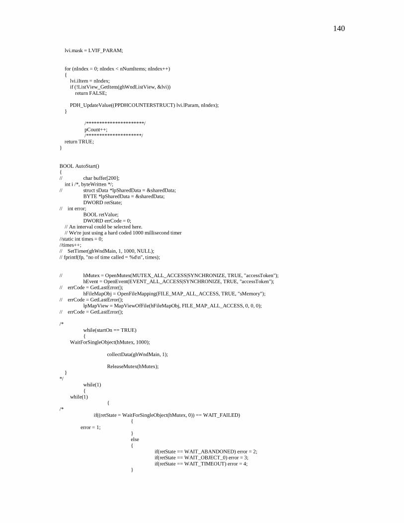
140

lvi.mask = LVIF_PARAM;

for (nIndex = 0; nIndex < nNumItems; nIndex++){

lvi.iItem = nIndex;if (!ListView_GetItem(ghWndListView, &lvi))

return FALSE;

PDH_UpdateValue((PPDHCOUNTERSTRUCT) lvi.lParam, nIndex);}

/**********************/pCount++;/*********************/

return TRUE;}

BOOL AutoStart(){// char buffer[200];

int i /*, byteWritten */;// struct sData *lpSharedData = &sharedData;

BYTE *lpSharedData = &sharedData;DWORD retState;

// int error;BOOL retValue;DWORD errCode = 0;

// An interval could be selected here.// We're just using a hard coded 1000 millisecond timer

//static int times = 0;//times++;// SetTimer(ghWndMain, 1, 1000, NULL);// fprintf(fp, "no of time called = %d\n", times);

// hMutex = OpenMutex(MUTEX_ALL_ACCESS|SYNCHRONIZE, TRUE, "accessToken");hEvent = OpenEvent(EVENT_ALL_ACCESS|SYNCHRONIZE, TRUE, "accessToken");

// errCode = GetLastError();hFileMapObj = OpenFileMapping(FILE_MAP_ALL_ACCESS, TRUE, "sMemory");

// errCode = GetLastError();lpMapView = MapViewOfFile(hFileMapObj, FILE_MAP_ALL_ACCESS, 0, 0, 0);


/*while(startOn == TRUE){

WaitForSingleObject(hMutex, 1000);


ReleaseMutex(hMutex);}

*/while(1){

while(1){

/*if((retState = WaitForSingleObject(hMutex, 0)) == WAIT_FAILED)

{error = 1;

}else{

if(retState == WAIT_ABANDONED) error = 2;if(retState == WAIT_OBJECT_0) error = 3;if(retState == WAIT_TIMEOUT) error = 4;

}

141

*/retState = WaitForSingleObject(hEvent, 1000);

retValue = ResetEvent(hEvent);// retValue = ReadFile(hFileMap, lpSharedData, sizeof(sharedData), &byteWritten, NULL);

lpSharedData = &sharedData;/*


(BYTE)*lpSharedData = lpMapView[i];(BYTE)lpSharedData++;

}*/



}

if(sharedData.nextProcess == PDH_App)break;

// retValue = ReleaseMutex(hMutex);retValue = SetEvent(hEvent);

//** might put delay here **Sleep(1);

}

lpSharedData = &sharedData;for(i=0; i<sizeof(BOOL); i++)

{(BYTE)*lpSharedData = lpMapView[i];(BYTE)lpSharedData++;

}

lpSharedData = &sharedData;lpSharedData += sizeof(BOOL);lpSharedData += sizeof(int);

for(i=0; i<SIZE*sizeof(char); i++){

(BYTE)*lpSharedData = lpMapView[sizeof(BOOL)+sizeof(int)+i];(BYTE)lpSharedData++;

}


sharedData.nextProcess = FTP_App;// WriteFile(hFileMap, lpSharedData, sizeof(sharedData), &byteWritten, NULL);

lpSharedData = &sharedData;lpSharedData += sizeof(BOOL);

for(i=0; i<sizeof(int); i++){

lpMapView[sizeof(BOOL)+i] = (BYTE)*lpSharedData;(BYTE)lpSharedData++;

}

/*lpSharedData = &sharedData;



}*/

if(sharedData.doneFlag == TRUE)break;

// retValue = ReleaseMutex(hMutex);retValue = SetEvent(hEvent);

142

Sleep(1);}

/*sharedData.nextProcess = FTP_App;

// WriteFile(hFileMap, lpSharedData, sizeof(sharedData), &byteWritten, NULL);



}*/

fp = fopen("pdhData.log", "a");




}

UnmapViewOfFile(lpMapView);CloseHandle(hFileMapObj);

fclose(fp);// ReleaseMutex(hMutex);

retValue = SetEvent(hEvent);// CloseHandle(hMutex);

return TRUE;}

BOOL AutoStop(){

// Kill the timer// KillTimer(ghWndMain, 1);

return TRUE;}

Change made in pdhfns.c

BOOL PDH_DisplayFormattedValue(/***LONG**/ DOUBLE lValue, int nItemIndex, int nSubItem){

TCHAR szMsg[1024];

/** change **wsprintf(szMsg, TEXT("%d"), lValue);fprintf(fp, "%d ", lValue);

*//*

wsprintf(szMsg, TEXT("%d"), (LONG)lValue);fprintf(fp, "%2.2f ", lValue);

*/if(nItemIndex == 0)

dataArray[pCount].counter1 = lValue;if(nItemIndex == 1)

dataArray[pCount].counter2 = lValue;if(nItemIndex == 2)

dataArray[pCount].counter3 = lValue;

SetSubItemText(nItemIndex, nSubItem, szMsg);

return TRUE;}

143

BOOL PDH_UpdateValue(PPDHCOUNTERSTRUCT pCounterStruct, int nItemIndex){

BOOL fRes = TRUE;PDH_FMT_COUNTERVALUE pdhFormattedValue;

__try {

if (ERROR_SUCCESS != PdhGetFormattedCounterValue(pCounterStruct->hCounter,

/**change** PDH_FMT_LONG, ***/PDH_FMT_DOUBLE,NULL,&pdhFormattedValue )) {

UpdateStatus(TEXT("Failure in PdhGetFormattedCounterValue."));fRes = FALSE;

}}__except(EXCEPTION_EXECUTE_HANDLER) {

UpdateStatus(TEXT("Exception in PdhGetFormattedCounterValue. (Handled)"));MessageBeep(0);fRes = FALSE;

}

if (fRes) {if (pdhFormattedValue.CStatus != ERROR_SUCCESS) {

// error in the counter// report the error in the list viewSetSubItemText(nItemIndex, COL_COUNTERVALUE, TEXT("Error"));fRes = FALSE;

}else

PDH_DisplayFormattedValue(/**change **pdhFormattedValue.longValue ***/ pdhFormattedValue.doubleValue,nItemIndex, COL_COUNTERVALUE);

}

return fRes;}

Modification on the makefile of the NcFTP application

CC=cl.exe -nologoLINK=link.exe -nologo

!ifdef DEBUGCFLAGS= -Od -Z7 -D_DEBUG -D_CONSOLE -DWIN32 -DDIRECT -DDOMAINNAME=\"foo.com\" -I. -Ih:\slo\ncftp-orig\pdcurses-2.3b-win32LINKFLAGS= -nologo -debug -pdb:none -subsystem:console!elseCFLAGS= -Od -DNDEBUG -DWIN32 -DDIRECT -DDOMAINNAME=\"foo.com\" -I. -Ih:\slo\ncftp-orig\pdcurses-2.3b-win32LINKFLAGS= -nologo -release -subsystem:console!endif

ENTRYPOINT=

LIBS=h:\slo\ncftp-orig\pdcurses-2.3b-win32\win32\pdcurses.lib h:\slo\ncftp-orig\ncftp-2.4.2-win32\pdh.lib user32.lib wsock32.lib

OBJS = simplePerf.obj\bookmark.obj\cmdline.obj\cmdlist.obj\cmds.obj\complete.obj\cpp.obj\datesize.obj\ftp.obj\

144

get.obj\getopt.obj\glob.obj\hostwin.obj\lgets.obj\linelist.obj\list.obj\macro.obj\main.obj\makeargv.obj\open.obj\prefs.obj\progress.obj\put.obj\rcmd.obj\sio.obj\strn.obj\tips.obj\util.obj\wgets.obj\win.obj\win32.obj\xfer.obj

all: ncftp.exe

ncftp.exe: $(OBJS)$(LINK) $(LINKFLAGS) @<<

$(OBJS) -out:ncftp.exe $(LIBS)<<

config.h: Config.h.w32copy Config.h.w32 config.h

sys.h: win32.h Util.h Main.h Cmds.h Open.h Cmdline.h DateSize.h Prefs.h FTP.h Getopt.hXfer.h Tips.h Version.h config.h simplePerf.h pdh.h

touch sys.h

simplePerf.obj: simplePerf.c simplePerf.h pdh.h

bookmark.obj: bookmark.c sys.h util.h bookmark.h ftp.h

cmdline.obj: cmdline.c sys.h Util.h Cmdline.h Cmds.h Main.h MakeArgv.h Open.h

cmdlist.obj: cmdlist.c Curses.h Util.h Main.h Open.h Cmds.h Glob.h List.h Get.h Put.hHostwin.h Prefs.h Cmdline.h

cmds.obj: cmds.c sys.h Util.h RCmd.h Cmds.h Cmdline.h List.h MakeArgv.h Macro.h Main.hDateSize.h Open.h Glob.h Getopt.h FTP.h Cpp.h Prefs.h Tips.h Version.h

complete.obj: complete.c sys.h LineList.h Cmdline.h Complete.h Prefs.h Util.h List.h

cpp.obj: cpp.c sys.h Curses.h Util.h RCmd.h Cpp.h

datesize.obj: datesize.c sys.h Util.h RCmd.h Cmds.h Xfer.h List.h DateSize.h

ftp.obj: ftp.c sys.h Util.h FTP.h RCmd.h

get.obj: get.c Util.h RCmd.h Xfer.h Cmds.h Glob.h Get.h DateSize.h List.h Getopt.h sys.h

getopt.obj: getopt.c sys.h util.h getopt.h

glob.obj: glob.c sys.h Util.h RCmd.h Glob.h Xfer.h List.h Main.h

hostwin.obj: hostwin.c sys.h curses.h Util.h Cmds.h Open.h Hostwin.h

lgets.obj: lgets.c sys.h util.h lgets.h

list.obj: list.c sys.h Util.h RCmd.h Xfer.h Cmds.h List.h Glob.h

145

linelist.obj: linelist.c sys.h

macro.obj: macro.c sys.h Util.h Macro.h Cmds.h Cmdline.h MakeArgv.h

main.obj: main.c sys.h

makeargv.obj: makeargv.c sys.h util.h makeargv.h

open.obj: open.c sys.h Open.h Util.h GetPass.h Cmds.h RCmd.h FTP.h Get.h Getopt.h Macro.hHostwin.h Main.h

prefs.obj: prefs.c sys.h curses.h wgets.h Util.h Cmds.h Progress.h Hostwin.h Prefs.hRCmd.h Main.h

progress.obj: progress.c sys.h Util.h Cmds.h Xfer.h Progress.h GetPass.h Main.h curses.h

put.obj: put.c sys.h Util.h RCmd.h Xfer.h Cmds.h Get.h Getopt.h Glob.h Put.h

rcmd.obj: rcmd.c sys.h Util.h RCmd.h Open.h Main.h Xfer.h FTP.h

sio.obj: sio.c sys.h sio.h

strn.obj: strn.c sys.h strn.h

tips.obj: tips.c sys.h util.h tips.h

util.obj: util.c sys.h Util.h Main.h Curses.h

wgets.obj: wgets.c sys.h util.h curses.h

win.obj: win.c sys.h Util.h Main.h Version.h RCmd.h LGets.h GetPass.h

win32.obj: win32.c win32.h

xfer.obj: xfer.c sys.h Util.h Main.h Xfer.h RCmd.h FTP.h Progress.h Sio.h

####### Maintainance Targets######

clean:-del *.obj-del *.tr2-del *.exe-del *.td2

performance measurement of network applicationjharris/3comproject/masters... · performance...

Documents