performance of agriculture in river basins of tamil nadu in the last
TRANSCRIPT
1
Performance of Agriculture in River Basins of Tamil Nadu
In the last three Decades – A Total Factor Productivity
Approach
A Project Sponsored by Planning Commission,
Government of India
Research Team
K.Palanisami
C.R.Ranganathan
A.Vidhyavathi
Rajkumar.M
N.Ajjan
Final Report
March 2011
Centre for Agricultural and Rural Development Studies
Tamil Nadu Agricultural University
Coimbatore – 641 0013
2
Acknowledgement
The authors express their sincere thanks to Planning Commission, Government of
India for providing necessary financial support to carry out this study. The authors
express their sincere thanks to Tamil Nadu Agricultural University for providing
necessary facility to carry out the research work.

3
CONTENTS
S.No CHAPTER Topics Page
No.
1 I 1. Executive Summary 1
2 II 2. Introduction 7
3
III
3. Objectives 10
3.1. Review of Past Studies: TFP measures
4 IV
4. Data Envelopment Analysis (DEA) 17
4.1. Input and output orientations
5
V
5. Profile of the Study Area: Tamil Nadu
27
5.1. Principal crops and production
5.2. Irrigation
5.3. Problems facing Agriculture in the State
5.3.1. Land degradation and soil quality
5.3.2. Wastelands
5.3.3. Pollution
6 VI 6. Profile of River Basins of Tamil Nadu 35
7
VII
7. Methodology
38
7.1. Estimation of basin areas and proportion of
basin areas in each district of Tamil Nadu
7.2. Conversion of district-wise data to basin-wise
7.3. Estimation of Malmquist Index of Total Factor
Productivity Growth in Agriculture
7.4. The Malmquist TFP Index
8 VIII
8. Basin coverage 44
8.1. Time period
9
IX
9. Output Series
9.1. Total inputs
45 9.1.1. Labor Input
9.1.2. Land Input

4
S.No CHAPTER Topics Page
No.
9.1.3. Chemical Fertilizer input
9.1.4. Irrigation Input
9.1.5. Livestock inputs
9.1.6. Units of variables
10
X
10. Results and Discussions
47
10.1. Summary Statistics
10.1.1. Crop output
10.1.2. Livestock output
10.1.3. Net Sown Area and net irrigated area
10.1.4. Fertilizer Usage
10.1.5. Labour input
10.1.6. Cattle and poultry input
11 XI
11. Liberalization policies and their effects on
agriculture in the river basins 56
12 XII
12. Comparison of crop out per unit of sown area
and per unit of water potential 67
13
XIII
13. Results of TFP analysis
71 13.1. Overall TFP growth
13.2. Individual basin TFP
13.3. Growth rates of TFPs
14 XIV 14. Cumulative TFP indices 82
15
XV
15. Results of DEA analysis
86
15.1. DEA with VRS technology and Output
Orientation.
15.2. DEA with VRS technology and Input
Orientation.
16 XVI 16. Summary and Conclusion 94
17 XVII 17. Policy recommendations 98
18 XVIII 18. References 100

5
LIST OF TABLES
Table
No List of Tables
Page
No
1 Total Factor Productivity trends for crops in selected states 13
2 Land Use Pattern in Tamil Nadu (Lakh ha) 28
3 Land Holding Pattern in Tamil Nadu 29
4 Status of Principle Crops in Tamil Nadu 30
5 Reduction in Per Capita Availability of Water in Tamil Nadu
31 6 Season wise Rainfall in Tamil Nadu (mm)
7 Irrigation Status in Tamil Nadu ( Area in lakh ha)
8 Change in Availability of Groundwater in Tamil Nadu 32
9 Major River Basins of Tamil Nadu 35
10 Area and Rainfall of the River Basins 36
11 Surface and Groundwater Potential of the River Basins 37
12 Summary Statistics Crop output (Rs.Crores) 47
13 Summary Statistics - Livestock output (Rs.Crores) 51
14 Summary Statistics - Net-Area-Sown-Input (Area in ha) 52
15 Summary Statistics - Net Irrigated Area Input (Area in ha) 53
16 Summary Statistics - NPK-Value-Input (in lakh tonnes)
17 Summary Statistics - Labour input (in Numbers) 54
18 Summary Statistics - Cattle-Input (in Numbers) 55
19 Summary Statistics - Poultry-Input (in Numbers)
20 Crop output (Rs. In crores) in the pre and post liberalization periods 57
21 Livestock output (Rs. In Crores) in the pre and post liberalization periods 59

6
Table
No List of Tables
Page
No
22 Net area sown (Area in ha) in the pre and post liberalization periods 60
23 Net area irrigated input (Area in ha) in the pre and post liberalization periods 61
24 N, P, K input (in lakh tonnes) in the pre and post liberalization periods 62
25 Labour input (number) in the pre and post liberalization periods 63
26 Cattle input (number) in the pre and post liberalization periods 64
27 Poultry input (number) in the pre and post liberalization periods 65
28 Value of crop output per ha. of sown area 67
29 Value of crop output per MCM of water potential 69
30 Mean Technical Efficiency Change, Technical Change and TFP Change, during
three decades in the seventeen river basins of Tamil Nadu 75
31 Table Mean TFPs in three periods 77
32 Growth rates of TFPs 80
33 Output Oriented VRS DEA model scores for the River basins of Tamil Nadu 87
34 Output Oriented VRS DEA model –benchmarks and projected values 89
35 Input Oriented VRS DEA model scores for the River basins of Tamil Nadu 91
7
LIST OF FIGURES
Figure
No List of Figures Page No
1 Map of Tamil Nadu State 27
2 River Basins of Tamil Nadu 35
3 Crop output in Small Basins during 1975-76 to 2005 - 06 48
4 Crop output in Medium Basins during 1975-76 to 2005 – 06 49
5 Crop output in Large Basins during 1975-76 to 2005 - 06 50
6 Crop output/ ha of net sown area 68
7 Crop output/per unit of water 70
8 Trend in Total Factor Productivity Index in Small basins during 1975-
76 to 2005 - 06 72
9 Trend in Total Factor Productivity Index in Medium basins during
1975-76 to 2005 - 06 73
10 Trend in Total Factor Productivity Index in Large basins during 1975-
76 to 2005 - 06 74
11 Cumulative TFP Indices in Small basins during 1975-76 to 2005 – 06 83
12 Cumulative TFP Indices in Medium basins during 1975-76 to 2005 – 06 84
13 Cumulative TFP Indices in Large basins during 1975-76 to 2005 - 06 85

8
CHAPTER I
Executive Summary
1. Introduction/Objectives
Tamil Nadu has 17 major river basins and most of them are water stressed. Agricultural
sector consumes about 75% of the water resources. Agriculture sector faces major constraints due
to water scarcity. There is growing demands for water from industry and domestic users and also
interstate competition for surface water resources also intensifies. Given the state water policy,
priority is given for domestic use followed by irrigation and industry etc. indicating that
agricultural sector has to manage the scarcity in the future. Further the canal systems have poor
water control and management. Also, out of the 1.8 million wells, about 0.16 million wells are
defunct in the state as the water table is fast declining. Again, out of the 385 blocks in the state,
90 are dark (extraction exceeding 100% of the recharge, 89 are grey (extraction exceeding 65%)
and the rest are white where the extraction is less than 65%.
Given all these constraints and scarcities for the existing water supply scenarios, what is
needed is the clear understanding of the value of water in alternate uses as well as the incentive to
allocate the water among competing crops and uses in different river basins. However, currently
the available information is related to the administrative boundaries such as districts, which as
such are difficult to relate with the river basin boundaries. Hence, it is important to reorient the
district level data to basin level for making basin level interventions. This will also help to work
out the performance of both irrigation and agriculture sectors at basin level.
Accordingly the main objectives of the study are as follows:
i) To analyze the agricultural growth in all the 17 river basins of Tamil Nadu using the
total factor productivity approach,
ii) To study the income inequality in all the river basins of Tamil Nadu, and
iii) To suggest policy options to improve the productivity of agriculture in the basins.
iv) To assess the performance of agriculture, apart from growth rates, total factor
productivity (TFP) was mainly used employing Data Envelopment Analysis (DEA).
These objectives are set with a view to provide guidance in policy planning in river
basins. Since the main objective of the study is to study agricultural growth in major river
basins, historical data on agricultural production for the past three decades were used.
District-wise data on agricultural production available from various government
publications are the primary data for the present study.

9
1.1. Methodology
All the 17 river basins of Tamil Nadu constituted our study area. They were Chennai
basin, Palar basin, Varahanadhi basin, Ponnaiyaar basin, Vellar basin, Paravanar basin, Cauvery
basin, Agniyar basin, Pambar and Kottakaraiyar basin, Vaigai basin, Gundar basin, Vaippar
basin, Kallar basin, Thambaraparani basin, Nambiar basin, Kodaiyar basin and Parambikulam
Azhiyar Project (PAP) basin. The study covers the period of 1975 -76 and 2005 -2006, which
concerned with important changes in agriculture due to liberalization of trade and reforms in
investment, initiation of privatization, tax reforms and inflation controlling measures. The study
used two output variables, viz., crops and livestock output variables. The output series for these
two variables were derived by aggregating detailed output quantity data of all agricultural
commodities. Area under each crop was multiplied by the constant prices of respective crop to
arrive at agricultural output. Total inputs use in agriculture included of labor, land, chemical
fertilizers, and irrigation area were used.
The district-wise data was first converted into basin-wise data based on the area of each
basin falling under each district. Total factor productivity (TFP) for each basin for each year was
computed using Malmquist index methods. This approach employs data envelopment analysis
(DEA) which a non-parametric method. The Malmquits index is computed by using the formula
,
,
,
,
,,,,
2/1
ssto
ttto
ssso
ttso
ttssoxyd
xydx
xyd
xydxyxym
Where the notation ),( ttso yxd represents the distance from the period t observation to the
period s technology. A value of mo greater than one will indicate positive TFP growth from
period s to period t while a value less than one indicates a TFP decline. These distance functions
are obtained by solving linear programming models derived from DEA methodology.
1.2. Findings/Conclusions
There was wide range of crop and livestock outputs in all the river basins. Though net
irrigated area increased over the decades, there was not much increase in net sown area. This
was supported by the minimum of coefficient of variation. In addition, there was considerable
increase in intake of NPK fertilizers in all river basins.
As the decades under consideration were after green revolution, the intake of inorganic
fertilizers had increased due to increase in area under high yielding varieties and area under

10
irrigation. There was tremendous increase in poultry population in Tamil Nadu especially in
Cauvery basin and P.A.P basin. Only after 1990s, there was wide fluctuation in crop output in
all the river basins. Before 1990s, the trend was smooth. The same trend was also noted in
livestock output.
Though net irrigated area has shown positive trend in pre liberalization period and
negative trend in post liberalization period, the net sown area has sown negative trend invariably
in both the periods in all basins. As expected net irrigated area was increasing at declining rate
over the decades. After post liberalization period, the trend was vigorous. This was mainly due
to proliferation of wells particularly bore wells.
NPK consumption in agriculture was increasing at decreasing rate. Increase in net
irrigated area has led to increased consumption of fertilizers. After liberalization period, change
in labour use in agriculture was negative in few basins and was less in other basins compared to
pre liberalization period. In pre liberalization period there was positive percentage change in all
river basins. Comparing cattle input in base year and current year period, Tamil Nadu as a whole
showed negative change. In general, poultry population was increasing over the decades.
The total factor productivity indices of 17 river basins fluctuate during the whole period
of study. Technical efficiency change was further decomposed into pure efficiency change and
scale efficiency change. The TFP analysis showed that in Chennai basin agricultural production
is technically efficient as the TFP was more than 1. In Palar basin the range of efficiency change
was from 0.772 to 1.506. There was not much difference in TFP and other efficiency change in
pre liberalization period and post liberalization period.
It was more than one indicating that Palar basin was technically efficient in using inputs.
In Varahanadhi basin TFP was more than one in pre and post liberalization periods indicating
that the basin was technically sound. Though in Ponnaiyaar river basin average TFP was more
than one, in post liberalization period it was less than one i.e. 0.957. In pre liberalization period,
it was 1.229.
In Paravanar basin, the average TFP was 1.034 and there was slight difference in TFP in
pre (0.989) and post liberalization period (1.079). The efficiency change was one in both periods
and the change in TFP was due to technical efficiency change.
In Vellar basin the average TFP was more than one (1.070) in the last three decades.
There was no difference noted in pre and post liberalization periods. Nevertheless, the efficiency
change was less than one and the technical change was more than one. The average TFP was
nearing one in post libralisation period and it was above one in pre liberalization period (1.115).
11
Though technical change was more than one in both periods, the efficiency change was less than
one or nearing one.
There is a possibility for improving efficiency of inputs in Agniyar basin as there was
slight reduction in efficiency change from 1.013 (pre liberalization period) to 0.986 (post
liberalization period). Though average TFP was more than one in both periods in Pambar &
Kottakaraiyar river basin, there was slight reduction in TFP and technical change in post
liberalization period.
The same trend was noted in Vaigai basin as in case of Pambar & Kottakaraiyar basin.
Gundar river basin also followed the same trend as that of Pambar and Vaigai basin. The
average TFP for the last three decades was 0.99. In Kallar basin the changes in total factor
productivity was mainly due to technical change. As efficiency change was 1 and there was no
change in efficiency of inputs in last three decades, any development activity should focus on
technical improvement. In Nambiar basin changes in total factor productivity was fully
contributed by technical changes and not due to the efficiency of inputs in agriculture and allied
sector. There was no change in TFP in two periods indicating that there was not much change in
technology adopted by the farmers. Efficiency of inputs also needs attention, as it remained
same in both the periods. In Kodaiyar basin also changes in total factor productivity was fully
contributed by technical changes and not due to the efficiency of inputs in agriculture and allied
sector.
P.A.P was the only basin in which the total factor productivity was less than one in pre
and post liberalization period. The average total factor productivity was 0.976 for the last three
decades.
All river basins had shown negative growth rate in pre liberalization period except P.A.P
basin. In post liberalization period basins, namely Chennai, Palar, Varahanadhi, Ponnaiyaar,
Paravanar, Vaippar, Thambaraparani and Nambiar river basins have shown positive growth rate.
All other river basins showed negative growth rate in post liberalization period. The positive
growth rate was mainly due to efficiency of inputs used for agriculture and livestock.
Efficiency change has contributed much to the total factor productivity. But overall
growth rate ie growth rate of total factor productivity for last three decades was negative for all
river basins except Nambiar and P.A.P river basins. However, most of the river basins have
shown total factor productivity more than one but there was no growth in the total factor
productivity in last three decades except in one or two basins.

12
1.3. Recommendations
1. Since crop and livestock are the integral components of agricultural production, it is
important to make developmental programs to be converging at basin level. All the ongoing and
proposed programs should have common linkages and aim to deliver the target output.
Livestock is the major supplementary income for farming community. As the number of
animals maintained by a farm firm is merely for meeting domestic needs and meeting daily
expenses. Dairying is not done as commercial activities by all farms. Farmers should be
encouraged to practice dairying as commercial venture by providing technical guidance and
credit facilities. Development of poultry industry in agricultural farms could lead to more area
under maize and other cereals and development of feed units. Training and technical expertise in
dairying and poultry will sustain marginal and small farming communities in Tamil Nadu.
2. The results of the DEA and TFP analyses help to identify the basins for efficient use of
the resources. Increasing the cropping and irrigation intensity will help some of the basins to
perform comparatively well. Hence using the results of the study the basins that have more
potential to improve the performance through efficient use of the resources such as water,
labour, fertilizer should be identified and interventions should be made to improve the
performance.
3. Technology package should be updated and made available for each basin and the cost
of transfer and adoption should be linked with the ongoing programs. Needed capacity building
programs should be in built using the existing KVKs and regional agricultural research stations.
4. Conservation programs such as watershed management and improved water
management techniques such as drip and sprinklers are still lacking behind due to poor
adoption. Future water related investment programs should therefore aim to develop strategies
and action plans to address the issue of efficient water allocation and management with the goal
of maximizing the productivity per unit of water. Given the existing water supply scenarios, the
demand management strategies will be considered more relevant for the efficient management
of the available supplies. Therefore, what is needed is the clear understanding of the value of
water in alternate uses as well as the incentive to allocate the water among competing crops and
uses in different river basins.

13
5. Creation of strong database at basin level is important incorporating the supply and
demand details of water crop, and livestock. Investment made, returns to investment in various
activities in the basin should be documented and analyzed periodically for making future
projects of the basin current and future potential.
6. Climate change will affect the water supplies and it is important to identify and
implement the various adaptation measures at both micro (farm) level and macro (basin) level.
This will help to improve the overall basin performance.

14
CHAPTER II
Introduction
2. Introduction
Tamil Nadu's geographic area consists of 17 river basins, a majority of which is water-
stressed. There are 61 major reservoirs; about 40,000 tanks and about 3 million wells that heavily
utilize the available surface water (17.5 BCM) and groundwater (15.3 BCM). Agriculture is the
single largest consumer of water in the State, using 75% of the State's water. Agriculture sector
faces major constraints due to dilapidated irrigation infrastructure coupled with water scarcity
due largely to growing demands from industry and domestic users and intensifying interstate
competition for surface water resources. In some parts of the state, the rate of extraction of
groundwater has exceeded recharge rates, resulting in falling water tables.
Water quality is also a growing concern. Effluents discharged from tanneries and textile
industries and heavy use of pesticides and fertilizers have had a major impact on surface water
quality, soils, and groundwater. The State Government has taken a number of progressive actions
on water resources and irrigation management, particularly through the World Bank-assisted
Tamil Nadu Water Resources Consolidation Project (WRCP). Tamil Nadu was one of the first
states to pass a groundwater bill, Procurement/Right to transparency act and a farmer‟s
management of irrigation systems acts. The State has prepared a planning framework for water
resources management, and a State Water Policy.
Given the geographical area of about 13 m.ha and the average annual rainfall of about
950 mm with bi-modal distribution, the surface water potential is estimated at 25000 MCM (893
TMC) and the ground water potential is about 22400 MCM (800 TMC). The demand for non-
agricultural purposes in year 2025 will be about 16500 MCM (589 TMC) and the demand for
agriculture purposes will be about 45000 MCM (1607 TMC) thus leaving a supply-demand gap
of about 14100 MCM (504 TMC) (29.7 %). Given the state water policy, priority is given for
domestic use followed by irrigation and industry etc. indicating that agricultural sector has to
manage the scarcity in the future.
The major issues with the canal systems are poor water control and management, inter-
sectoral water demand and the crop pattern with high water intensive crops such as rice,

15
sugarcane, banana, and turmeric. The irrigation efficiency is ranging from 40 to 50% only.
Compared to the annual operation & maintenance expenditure of about Rs 400 million,
The cost recovery is only about Rs.100 millions indicating poor maintenance of the
systems. In the case of tanks, the major issues are tank siltation, encroachment, poor system
management, and heavy dependence on rice cultivation. Out of 39200 tanks in the state, about 2
% are defunct in the tank intensive regions and about 67% in the tank-non intensive regions. This
is because, in a 10-year period, the tanks fill fully only in 2 years, partially fill in 5 years and fail
in 3 years. Mostly marginal and small farmers are distributed in the tank commands.
Water market is getting importance in the recent years mainly to supplement the
inadequate tank water particularly at the end of the rice crop period. Farmers normally spent
about 20% of their rice crop income for buying water from wells owners. Since only about 15%
of the farmers own wells in the tank command, there is great demand for well water. However,
there is scope to diversify the crop pattern due to growing tank water scarcity. In the case of
wells, the wells in the canal and tank commands perform well compared to non-command areas,
due to declining water table. Out of the 1.8 million wells, about 0.16 million wells are defunct in
the state as the water table is fast declining. Out of the 385 blocks in the state, 90 are dark
(extraction exceeding 100% of the recharge, 89 are grey (extraction exceeding 65%) and the rest
are white where the extraction is less than 65%. The average area irrigated per well has decreased
from 1.4 ha during 1980s to 0.4 during 1990s indicating the water scarcity due to high well
density and the associated well failure. The imputed cost of providing irrigation through wells is
about Rs 0.3 million per ha. Further the flat rate of electricity from 1984 onwards and the free
electricity introduced in the state from 1989 onwards also to some extent contributed for the
over-exploitation of the ground water.
The efficiency of the irrigation systems are also reflected in the productivity of crops per
unit of water. Mostly crops under well irrigation systems are giving higher productivity per unit
of water.
The inter-sectoral water allocation is increasing in the recent years, as the wells, which
are the main sources of domestic water sources are failing due to declining water table and poor
water quality.
The industrial demand for water is also increasing where the water charges paid by the
industries form a sizeable portion of the O&M expenditure, thus indicating the scope for revenue
generation through efficient water allocation.
16
Government is making serious efforts in improving the performance of the irrigation
systems, through several interventions such as modernization of canal and tank irrigation
systems. In the case of regions with groundwater irrigation, watershed programs are introduced
in a big way.
Still, the performance of these systems is comparatively poor due to less incentive to
conserve water due to poor water control and management. The water users association formed
in the canal and tank commands under the WRCP have started functioning.
Conservation programs such as watershed management and improved water management
techniques such as drip and sprinklers are still lacking behind due to poor adoption. Future water
related investment programs should therefore aim to develop strategies and action plans to
address the issue of efficient water allocation and management with the goal of maximizing the
productivity per unit of water.
Given the existing water supply scenarios, the demand management strategies will be
considered more relevant for the efficient management of the available supplies. Therefore, what
is needed is the clear understanding of the value of water in alternate uses as well as the incentive
to allocate the water among competing crops and uses in different river basins. However,
currently the available information is related to the administrative boundaries such as districts,
which as such are difficult to relate with the river basin boundaries. Hence, it is important to
reorient the district level data to basin level for making basin level interventions. This will also
help to work out the performance of both irrigation and agriculture sectors at basin level.
Accordingly, the following objectives are set forth:
17
CHAPTER III
Objectives and Review of Literature
3. Objectives:
i) To analyze the agricultural growth in all the 17 river basins of Tamil Nadu using the total
factor productivity approach,
ii) To study the income inequality in all the river basins of Tamil Nadu, and
iii) To suggest policy options to improve the productivity of agriculture in the basins.
iv) To assess the performance of agriculture, apart from growth rates, total factor
productivity (TFP) was mainly used employing Data Envelopment Analysis (DEA).
3.1. Review of Past Studies: TFP measures
TFP growth shows the relationship between growth of output and growth of input,
calculated as a ratio of output to input. In other words, productivity is raised when growth in
output outpaces growth in input. Productivity growth without an increase in inputs is the best
kind of growth to aim for rather than attaining a certain level of output by increasing inputs, since
these inputs are subject to diminishing marginal returns. However, how to measure the total input
and total output is both conceptually and empirically difficult. Methods to estimate TFP can be
classified in four major groups:
1. least-squares econometric production models;
2. growth accounting TFP indices;
3. data envelopment analysis (DEA); and
4. Stochastic frontiers (Coelli et al., 2001).
The first two methods are normally used with times series data and assume that all
production units are technically efficient. Methods (3) and (4) can be applied to a cross-section of
firms, farms, regions, or countries to compare their relative productivity. In this study, we use
both a Törnqvist-Theil index (growth accounting framework) and a non-parametric Malmquist
index (DEA approach) to measure agricultural TFP growth in China and India.
The Malmquist index and based on distance functions, has become extensively used in
the measure and analysis of productivity after Färe et al. (1994) showed that the index can be

18
estimated using a non-parametric approach. The non-parametric Malmquist index has been
especially popular since it does not entail assumptions about economic behavior (profit
maximization or cost minimization) and therefore does not require prices for its estimation,
which in many cases are not available for international comparisons. Most important for this
study is its ability to decompose productivity growth into two mutually exclusive and exhaustive
components: changes in technical efficiency over time (catching-up) and shifts in technology
over time (technical change).
To define the output-based Malmquist index assume, as in Färe et al. (1998), that for each
time period t=1, 2…T the production technology describes the possibilities for the transformation
of inputs x t into outputs y
t .
This is the set of output vectors that can be produced with input vector x. For the
technology in period t and with y t ∈ mR
outputs and x
t ∈ nR inputs: The frontier of the output
possibilities for a given input vector is defined as the output vector that cannot be increased by a
uniform factor without leaving the set. In our analysis, we will refer to these production units as
basins. The output distance function is defined at t as the reciprocal of the maximum proportional
expansion of output vector y t
given input x t
. The distance measure equals 1 when the
production point in period t is on the frontier for period t.
The Malmquist index measures the TFP change between two data points (e.g. those of a
country in two different times) by calculating the ratio of the distance of each data point relative
to a common technological frontier. Following Färe et al. (1994), the Malmquist output-oriented
index between period t and t+1 is given by: as which is a geometric mean of two Malmquist
indices: one using the technology frontier in t as the reference, and a second index that uses
frontier in t+1 as the reference. Färe et al. (1994) showed that the Malmquist index could be
decomposed into an efficiency change component and a technical change component, and that
these results applied to the different period-based Malmquist indices. The ratio outside the square
brackets measures the change in technical efficiency between period t and t+1. The expression
inside brackets measures technical change as the geometric mean of the shift in the technological
frontier between t and t+1 evaluated using frontier at t and at t+1, respectively, as the reference.
The efficiency change component of the Malmquist indices measures the change in how
far observed production is from maximum potential production between period t and at t+1, and

19
the technical change component captures the shift of technology between the two periods. A
value of the efficiency change component of the Malmquist index greater than one means that the
production unit is closer to the frontier in period t+1 than it was in period t: the production unit is
catching-up to the frontier. A value less than one indicate efficiency regress. The same range of
values is valid for the technical change component of total productivity growth, meaning
technical progress when the value is greater than one and technical regress when the index is less
than one.
Research study done by Indian Institute of Agricultural Research, New Delhi indicated
that public investment in irrigation, infrastructure development (road, electricity), research and
extension and efficient use of water and plant nutrients were the dominant sources of TFP
growth. The sharp deceleration in total investment and more so in public sector investment in
agriculture is the main cause for the deceleration. This has resulted in the slow-down in the
growth of irrigated area and a sharp deceleration in the rate of growth of fertiliser consumption.
The most serious effect of deceleration in total investment has been on agricultural research and
extension. This trend must be reversed as the projected increase in food and non-food production
must accrue essentially through increasing yield per hectare. Recognising that there are serious
yield gaps and there are already proven paths for increasing productivity. It is very important for
India to maintain a steady growth rate in total factor productivity. As the TFP increases, the cost
of production decreases and the prices also decrease and stabilise. Both producer and consumer
share the benefits.
The fall in food prices will benefit the urban and rural poor more than the upper income
groups, because the former spend a much larger proportion of their income on cereals than the
latter. All the efforts need to be concentrated on accelerating growth in TFP, whilst conserving
natural resources and promoting ecological integrity of agricultural system. More than half of the
required growth in yield to meet the target of demand must be met from research efforts by
developing location specific and low input use technologies with the emphasis on the regions
where the current yields are below the required national average yield.
Many observers have expressed concern that technological gains have not occurred in a
number of crops, notably coarse cereals, pulses and in rainfed areas. Recent analysis on TFP
growth based on cost of cultivation data does not prove this perception. Tamil Nadu has shown
increasing trend only in case of paddy. In all the 18 major crops considered in the analysis,
20
several states have recorded positive TFP growth. This is spread over major cereals, coarse
grains, pulses, oilseeds, fibres, vegetables, etc. In most cases, in the major producing states,
rainfed crops also, showed productivity gains. There is thus strong evidence that technological
change has generally pervaded the entire crop sector. There are, of course, crops and states where
technological stagnation or decline is apparent and these are the priorities for present and future
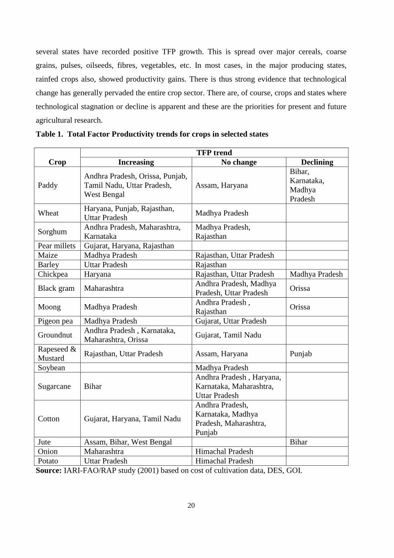
agricultural research.
Table 1. Total Factor Productivity trends for crops in selected states
Crop
TFP trend
Increasing No change Declining
Paddy
Andhra Pradesh, Orissa, Punjab,
Tamil Nadu, Uttar Pradesh,
West Bengal
Assam, Haryana
Bihar,
Karnataka,
Madhya
Pradesh
Wheat Haryana, Punjab, Rajasthan,
Uttar Pradesh Madhya Pradesh
Sorghum Andhra Pradesh, Maharashtra,
Karnataka
Madhya Pradesh,
Rajasthan
Pear millets Gujarat, Haryana, Rajasthan
Maize Madhya Pradesh Rajasthan, Uttar Pradesh
Barley Uttar Pradesh Rajasthan
Chickpea Haryana Rajasthan, Uttar Pradesh Madhya Pradesh
Black gram Maharashtra Andhra Pradesh, Madhya
Pradesh, Uttar Pradesh Orissa
Moong Madhya Pradesh Andhra Pradesh ,
Rajasthan Orissa
Pigeon pea Madhya Pradesh Gujarat, Uttar Pradesh
Groundnut Andhra Pradesh , Karnataka,
Maharashtra, Orissa Gujarat, Tamil Nadu
Rapeseed &
Mustard Rajasthan, Uttar Pradesh Assam, Haryana Punjab
Soybean Madhya Pradesh
Sugarcane Bihar
Andhra Pradesh , Haryana,
Karnataka, Maharashtra,
Uttar Pradesh
Cotton Gujarat, Haryana, Tamil Nadu
Andhra Pradesh,
Karnataka, Madhya
Pradesh, Maharashtra,
Punjab
Jute Assam, Bihar, West Bengal Bihar
Onion Maharashtra Himachal Pradesh
Potato Uttar Pradesh Himachal Pradesh
Source: IARI-FAO/RAP study (2001) based on cost of cultivation data, DES, GOI.

21
Talluri (2000) provides an introduction to DEA and some important methodological
extensions that have improved its effectiveness as a productivity analysis tool. They proposed a
combination of models that allowed for effective ranking of DMUs in the presence of both
quantitative as well as qualitative factors.
Other ranking methods that do not specifically include cross-efficiencies were proposed
by Rousseau and Semple (1995), and Andersen and Petersen (1993). Rousseau and Semple
(1995) approached the same problem as a two-person ratio efficiency game. Their formulation
provides a unique set of weights in a single phase as opposed to the two-phase approaches
presented above. Andersen and Petersen (1993) proposed a ranking model, which is a revised
version of problem. In this model, the test DMU is removed from the constraint set allowing the
DMU to achieve an efficiency score of greater than 1, which provides a method for ranking
efficient and inefficient units. He also discussed weight restrictions in DEA.
The study on total factor productivity of agricultural commodities in economic
community of West African states by Department of Agricultural Economics and Extension,
Ladoke Akintola University of Technology, Nigeria (2005) provided a view on extent of
productivity growth in crops relevant to food security and which have high potential for intra-
ECOWAS trade. This paper done so by obtaining measures of Total Factor Productivity (TFP)
for rice, cotton and millet over a 45-year period from 1961-2005 using a panel of major
ECOWAS countries producing the crops. Calculations were based on data collected from
FAOSTAT database, IRRI world rice statistics, international cotton advisory committee
database, and individual country statistical database and studies. The data included output of each
crop (rice, cotton and millet) and six input variables comprising land area, labour and seed
fertilizer and irrigation and country dummies.
The TFP measures were calculated using stochastic frontier approach. The TFP index was
obtained by simply multiplying the technical change and the technological change. This is
equivalent to the decomposition of the Malmquist index suggested by Fare et al (1994).The 45
year period is divided into two sub periods; 1961-1978 and 1979-2005 in order to study the
effects of ECOWAS reforms on productivity growth of the selected crops.
The results show evidence of phenomenal growth in the TFP of all the selected crops.
Cotton however has the most impressive results followed by rice. A closer look at the TFP in
ECOWAS and pre-ECOWAS sub-period shows larger TFP in ECOWAS period (1979-2005) for
rice, and millet but larger TFP in pre-ECOWAS period for cotton. In both periods, productivity
22
growth in rice and cotton was sustained through technological progress while it was sustained
through more efficient use of inputs in millet.
Olajide (2003) examined changes in agricultural productivity in Sub-Sahara Africa
countries in the context of diverse institutional arrangements using Data Envelopment Analysis
(DEA). From a time, series, which consists of information on agricultural production and means
of production, were obtained from FAO AGROSTAT and rainfall data from Steve O‟Connell
database. The information was for a 43-year period (1961-2003); DEA method was used to
measure Malmquist index of total factor productivity. A decomposition of TFP measures
revealed whether the performance of factors productivity is due to technological change or
technical efficiency change over the reference period. The study further examined the effect of
land quality, malaria, education and selected governance indicators such as, control of corruption
and government effectiveness on productivity growth. All the variables included in the model are
significant with the exception of government effectiveness. They equally performed well in terms
of expected relationship with TFP except education and land quality index, which unexpectedly
had an inverse relationship with TFP.
There are different methods for estimating the total factor productivity (TFP) growth e.g.
Malmquist and Tornquist indexes. The former had gained popularity in recent years since Fare et
al., (1994) apply the linear programming approach to calculate the distance functions that make
up the Malmquist index. According to Shih et al, (2003), since Data Envelopment Analysis
(DEA) type of analysis can be directly applied to calculate the index, the Malmquist index has
the advantage of computational ease, does not require information on cost or revenue shares to
aggregate inputs or outputs, consequently, less data demanding and it allows decomposition into
changes in efficiency and technology. This method does not attract any of the stochastic
assumptions restriction, however, it is susceptible to the effects of data noise, and can suffer from
the problem of „unusual‟ shadow prices, when degrees of freedom are limited (Coelli and Rao,
2003).
The issue of shadow prices is important and is one that is not well understood among
authors who apply these Malmquist DEA methods; also, DEA methods in measuring
productivity growth which made it distinct from pure index approach such as Fisher and
Tornkvist indexes is that it does not require any price data, more so that agricultural input price
data are seldom available and could at times be distorted by the government policies.

23
In the late 1970s, a mathematical programming approach known as Data Envelopment
Analysis (DEA) was developed to measure technical efficiency by comparing the individual
firm‟s production to the best practice frontier (Charnes, Cooper and Rhodes, 1978). The
contribution of Farrell was path breaking as noted by Forsund and Sarafoglou (2000) in their
article “On the origin of Data Envelopment Analysis”.
Efficiency measures were based on radial uniform contractions or expansions from
inefficiency observations to the frontier. Thomson and Thrall (1995) observed Farrell seminal
paper was followed by a relatively large number of refinement and extensions, which may be
broadly classified into three schools of thought and identified as Afriat School, Charnes School
and Shepherd School. Afriat School covers econometricians‟ parametric estimation approach,
while the last two may more accurately be termed axiomatic production theory school.

24
CHAPTER IV
Data Envelopment Analysis (DEA)
4. Data Envelopment Analysis (DEA)
DEA is linear-programming methodology, which uses data on input and output quantities
of a Decision Making Units (DMU) such as individual firms of a specific sectors to construct a
piece-wise linear surface over data points. In this study, the countries were used as the DMU.
The DEA method is closely related to Farrell‟s original approach (1957) and it is widely being
regarded in the literature as an extension of that approach. This approach was initiated by
Charnes et al.; (1978) and related work by Fare, Grosskopf and Lovell 1985) the frontier surface
is constructed by the solution of a sequence of linear programming problems. The degree of
technical inefficiency of each country, which represents the distance between the observed data
point and the frontier, is produced as a by-product of the frontier construction method.
Either DEA can be input or output oriented depending on the objectives. The input-
oriented method, defines the frontier by seeking the maximum possible proportional reduction in
input usage while the output is held constant for each country. The output-oriented method seeks
the maximum proportional increase in output production with input level held fixed. These two
methods, that is, input-output oriented methods provide the same technical efficiency score when
a constant return to scale (CRS) technology applies but are unequal when variable returns to
scale (VRS) is assumed (Coelli and Rao, 2001).
In this study, the output-oriented method will be used by assuming that in agriculture, it
is common to assume output maximization from a given sets of inputs. The interpretation of CRS
assumption has attracted a lot of critical discussion e.g. Ray and Desli, 1997, Lovell, 2001, but
also monotonicity and convexity are debatable e.g. Cherchye, et al., 2000.
Fare et al., (1994) used Data Envelopment Analysis (DEA) methods to estimate and
decompose the Malmquist productivity index. The DEA method is a non-parametric approach in
which the envelopment of decision-making units (DMU) can be estimated through linear
programming methods to identify the “best practice” for each DMU. The efficient units are
located on the frontier and the inefficient ones are enveloped by it.
A key advantage of DEA over other approaches previously examined is that it more
easily accommodates both multiple inputs and multiple outputs. As a result, it is particularly

25
useful for analysis of multispecies fisheries, because prior aggregation of the outputs is not
necessary. Further, as will be outlined below, a specific functional form for the production
process does not need to be imposed on the model (as is required in the use of the SPF approach).
The envelopment surface will differ depending on the scale assumptions that underpin the model.
Two scale assumptions are generally employed: constant returns to scale (CRS), and variable
returns to scale (VRS). The latter encompasses both increasing and decreasing returns to scale.
CRS reflects the fact that output will change by the same proportion as inputs are changed
(e.g. a doubling of all inputs will double output); VRS reflects the fact that production
technology may exhibit increasing, constant and decreasing returns to scale. As demonstrated in
Section 2.6, input- and output-based capacity measures are only equivalent under the assumption
of constant returns to scale. However, there are generally a priori reasons to assume that fishing
would be subject to variable returns and, in particular, decreasing returns to scale. Cooper,
Seiford and Tone (2000) provide a discussion of methods for determining returns to scale. In
essence, the researcher examines the technical efficiency given different returns to scale, and
determines whether the observed levels are along the frontier corresponding to a particular
returns to scale.
4.1. Input and output orientations
A range of DEA models have been developed that measure efficiency and capacity in
different ways. These largely fall into the categories of being either input-oriented or output-
oriented models.
With input-oriented DEA, the linear programming model is configured to determine how
much the input use of a firm could contract if used efficiently in order to achieve the same output
level. For the measurement of capacity, the only variables used in the analysis are the fixed
factors of production. As these cannot be reduced, the input-oriented DEA approach is less
relevant in the estimation of capacity utilization. Modifications to the traditional input-oriented
DEA model, however, could be done such that it would be possible to determine the reduction in
the levels of the variable inputs conditional on fixed outputs and a desired output level.
In contrast, with output-oriented DEA, the linear programme is configured to determine a
firm‟s potential output given its inputs if it operated efficiently as firms along the best practice
frontier. This is more analogous to the SPF approach, which estimated the potential output for a

26
given set of inputs and measured capacity utilization as the ratio of the actual to potential output,
and is consistent with the illustration of the method.
Coelli and Rao (2003) paper examined levels and trends in agricultural output and
productivity in 93 developed and developing countries that account for a major portion of the
world population and agricultural output. We make use of data drawn from the Food and
Agriculture Organization of the United Nations and our study covers the period 1980-2000. Due
to the non-availability of reliable input price data, the study uses data envelopment analysis
(DEA) to derive Malmquist productivity indexes. The study examines trends in agricultural
productivity over the period. Issues of catch-up and convergence, or in some cases possible
divergence, in productivity in agriculture are examined within a global framework. The paper
also derives the shadow prices and value shares that are implicit in the DEA-based Malmquist
productivity indices, and examines the plausibility of their levels and trends over the study
period. *This issue of shadow prices is important, and is one that is not well understood among
authors who apply these Malmquist DEA methods.
A major advantage cited in support of the use of DEA in measuring productivity growth,
is that these methods do not require any price data. This is a distinct advantage, because in
general, agricultural input price data are seldom available and such prices could be distorted due
to government intervention in most developing countries. However, an important point needs to
be added here. Even though the DEA-based productivity measures may not explicitly use market
price information, they do implicitly use shadow price information, derived from the shape of the
estimated production surface. This issue is described in some detail in Coelli and Prasada Rao
(2001), who show that one can use these shadow prices to calculate shadow shares information,
to help shed light on the factors influencing these productivity growth measures. Hence, a main
aim of this paper is to demonstrate the feasibility of explicitly identifying the implicit shadow
shares and to study regional variation and trends in these shares over time.
They used shadow share information to provide valuable insights into why various
authors have obtained widely differing TFP growth measures for some countries, when applying
these Malmquist DEA methods. This has been particularly evident when the applications have
involved panel data sets containing small groups of countries, and the countries included in each
data set differ from study to study.

27
Some important findings of the paper were on levels and trends in global agricultural
productivity over the past two decades. The results presented here examine the growth in
agricultural productivity in 93 countries over the period 1980 to 2000. The results show an
annual growth in total factor productivity growth of 2.1 percent, with efficiency change (or catch-
up) contributing 0.9 percent per year and technical change (or frontier-shift) providing the other
1.2 percent. This is most likely a consequence of the use of a different sample period and an
expanded group of countries.
In terms of individual country performance, the most spectacular performance is posted
by China with an average annual growth of 6.0 percent in TFP over the study period. Other
countries with strong performance are, among others, Cambodia, Nigeria and Algeria. The
United States has a TFP growth rate of 2.6 percent, whereas India has posted a TFP growth rate
of only 1.4 percent. Turning to performance of various regions, Asia is the major performer with
an annual TFP growth of 2.9 percent. Africa seems to be the weakest performer with only 0.6
percent growth in TFP.
Examining the question of catch-up and convergence, we find that those countries that
were well below the frontier in 1980 (with technical efficiency coefficients of 0.6 or below) have
a TFP growth rate of 3.6 percent. This was in contrast to a low 1.2 percent growth for the
countries that were on the frontier in 1980. These results indicate a degree of catch-up in
productivity levels between high-performing and low-performing countries. Those results were
quite interesting since they indicated an encouraging reversal during 1980-2000 period) in the
phenomenon of negative productivity trends and technological regression reported in some of the
earlier studies for the period 1961-1985.
Cheng Yuk-shing (1998) studied performance of Chinese agriculture and he used the
Malmquist index to examine the sources of productivity growth in Chinese agriculture. Since the
late 1980s, Chinese officials and economists had shown serious concern over the growth
potential of Chinese agriculture. Relative returns to agricultural activities have been conceived to
be too low and investment in agriculture insufficient. However, the fact was that China‟s
agriculture experienced a period of rapid growth in the 1990s, after a slow down in the second
half of the 1980s. In this study, Malmquist productivity indexes were computed for counties of

28
Jiangsu Province. They indicated that the total factor productivity growth in agriculture was as
high as 7.8% per annum during 1991-95.
The decomposition result showed that there was rapid technical progress, along with a
substantial decline in technical efficiency. This paper investigated the sources of productivity
growth in Chinese agriculture over the period of 1988-95, using county-level data of Jiangsu
Province. It had been shown that the growth of total factor productivity in 1991-95 was very
rapid, averaging 7.8% annually. Yet contribution of inputs to agricultural growth was negative
and technical efficiency declined substantially in this period. The productivity increase arose
from entirely technical progress.
The impressive technical progress may indicate that the efforts of the Chinese
government in boosting agricultural growth since the early 1990s might have been successful.
Policies conducive to agricultural growth include an increase in investment in agricultural and
irrigation facilities and an improvement in agriculture extensions. Output can be increased even if
the original factors of production are used. Still, another possibility is that farmers have shifted
their production more to cash crops that are high value-added products. In any case, further study
is needed in order to understand more about the remarkable technical progress in Chinese
agriculture.
However, the major challenge to Chinese agriculture is the decline in technical efficiency.
Previous studies suggest that there was substantial improvement in technical efficiency after the
introduction of household responsibility system in the early 1980s. The empirical result of this
study suggests that the efficiency level has not been maintained. The decline in efficiency in fact
has eroded part of the positive impact of the technical progress. For agricultural growth to sustain
in the future, the Chinese government might need to look more carefully into the factors that
have caused such a serious decline in efficiency.
Andre et al. showed a connection between Data Envelopment Analysis (DEA) and the
methodology proposed by Sumpsi et al. (1997) to estimate the weights of objectives for decision
makers in a multiple attribute approach in their working paper. This connection gave rise to a
modified DEA model that allows estimating not only efficiency measures but also preference
weights by radially projecting each unit into a linear combination of the elements of the payoff
matrix (which is obtained by standard multicriteria methods). For users of Multiple Attribute
Decision Analysis the basic contribution of this paper was a new interpretation of the
29
methodology by Sumpsi et al. (1997) in terms of efficiency. They also proposed a modified
procedure to calculate an efficient payoff matrix and a procedure to estimate weights through a
radial projection rather than a distance minimization. For DEA users, we provide a modified
DEA procedure to calculate preference weights and efficiency measures, which does not depend
on any observations in the dataset. This methodology has been applied to an agricultural case
study in Spain.
This connection could be exploited in order to suggest a modified version of DEA in
order to measure preference weights. The main idea is to use DEA including the elements of the
payoff matrix as the only units in the reference set and interpret the λ parameters as the weights
of each criterion or throughput. The purpose of this technique is to account for the effect of
technological (feasibility) constraints in the decision making process.
This way a single technique is capable of providing estimates of preference parameters
and an alternative efficiency measure with the property of being independent of the DMUs in the
sample. They had proposed a modified procedure to calculate the payoff matrix to guarantee that
all its elements are efficient.
Moreover, they provided an approximate measure of efficiency that depends only on the
information related to each DMU, being independent of the rest of the units in the sample. The
main drawback of the modified DEA model for DEA users is the calculation of the payoff
matrix, which usually requires full information about the decision problem that is faced by the
DMU‟s. In a further research, we are working on a way to avoid this difficulty.
Fan Shenggen et al (2009) measured and compared agricultural total factor productivity
(TFP) growth in China and India and relates TFP growth in each country to policy milestones
and investment in agricultural research.
TFP was measured using a non-parametric Malmquist index, which allows the
decomposition of TFP growth into its components: efficiency and technical change. The results
showed that comparing TFP growth in China and India it was found that efficiency improvement
played a dominant role in promoting TFP growth in China, while technical change had also
contributed positively. In India, the major source of productivity improvement came from
technical change, as efficiency barely changed over the last three decades, which explains lower
TFP growth than in China. Agricultural research had significantly contributed to improve

30
agricultural productivity in both China and India. Even today, returns to agricultural R&D
investments are very high, with benefit/cost ratios ranging from 20.7 to 9.6 in China and from
29.6 to 14.8 in India.
Rosegrant and Evenson (1995) assessed total factor productivity (TFP) growth in India,
examines the sources of productivity growth, including public and private investment, and
estimates the rates of return to public investments in agriculture. The results showed that
significant TFP growth in the Indian crops sector was produced by investments -- primarily in
research – but also in extension, markets, and irrigation. The high rates of return, particularly to
public agricultural research and extension, indicated that the Government of India was not
over investing in agricultural research and investment, but rather that current levels of public
investment could be profitably expanded.
Analysis of total factor productivity measured the increase in total output, which was not
accounted for, by increases in total inputs. The total factor productivity index was computed as
the ratio of an index of aggregate output to an index of aggregate inputs. Growth in TFP was
therefore the growth rate in total output less the growth rate in total inputs. In this analysis,
Tornqvist-Theil TFP indices were computed for 271 districts covering 13 states in India, 1956-
87.
Renuka Mahadevan (2003) assessed the productivity growth in Indian agriculture and to
study the impact of globalisation. The study revealed that, there could easily be benefits that have
not yet surfaced, or were yet to be identified and perhaps too difficult or intangible to measure.
Whatever the case, it was highly likely that it is too soon to assess the full impact of
globalization and economic reforms. Furthermore, the process of liberalization had been gradual
and remained incomplete.
For example, the complete removal of quantitative restrictions after March 2001 would
have provided an opportunity for Indian farmers to tap world markets and, if they were
successful, results should start to become evident soon. Export promotion via the development of
export and trading houses as well as effective liberalizing export promotion zone schemes for
agriculture were fairly recent measures and only time will tell as to how effective these measures
were. Other possibilities such as agro-industry parks for promoting exports were also in the
pipeline. In conclusion, India had successfully set sail on the waters of globalization and

31
economic reforms and even in the wake of economic and political instability, she had to carefully
steer her course in order to reap the benefits of increased productivity growth in the agricultural
sector.
Canan et al. (2008) analyzed productivity growth in Turkey, EU-15 and CEE (Central
and East European) Countries over the period 1995-2006. Malmquist productivity index had
been used to measure the productivity. A nonparametric programming method is used to compute
Malmquist productivity indexes, which were decomposed into two component measures, namely
technical change and efficiency change. It was found that Hungarian productivity growth was
higher than the other countries including EU-15 over the period 1995-2006, all with due to
efficiency change. Productivity growth in Turkey within the period analyzed decreased
especially in 2001, which was a crisis year.
Ramesh Chand (2005) measured the performance of agriculture sector in the country in
the recent years. The result turned out to be quite dissatisfactory because of sharp deceleration in
growth rate of agricultural output. Agricultural production over time was affected by interacting
influences of technological, infrastructural, and policy factors. During the decade of 1990s,
declining trend in public sector investment that set in year 1979-80 continued for most part of the
decade.
However, terms of trade were kept favourable to agriculture sector during 1990s by
hiking level of cereal prices through government support, trade liberalization, exchange rate
devaluation, and disprotection to industry.
Several researchers felt that as economic reforms focused mainly on price factor and
ignored infrastructure and institutional changes the overall impact on growth of agricultural
sector has not been favourable. Highest response to fertilizer was obtained in the case of Tamil
Nadu where one percent increase in fertilizer brought 0.7 percent increase in output. Elasticity of
crop output with respect to irrigation was one.
Tamil Nadu has scope to raise output by 0.65 and 0.82% per irrigation through irrigation.
Shift in one percent area from food grain to non-food grain offers scope to raise crop output by
1.73 percent in Uttar Pradesh 1.6 percent in Karnataka and Assam, 2.4 percent in Bihar 1.5
percent in Maharashtra, 1.4 Percent in West Bengal, 1.2 percent in Orissa and 1.1 percent in
Tamil Nadu. It seems likely that Andhra Pradesh, Bihar, Gujarat, Himachal Pradesh, Jammu and
Kashmir, Karnataka, Maharashtra, Orissa, Punjab, Tamil Nadu, U.P, and West Bengal are in a

32
position to increase fertilizer use by same rate as witnessed during 1990s. Expansion of area
under irrigation, improvement in total factor productivity, resource shift towards high value
enterprises and increase in application of fertilizer were the four sources of growth in agriculture.
Crop intensity is another source for output growth but in our exercise, its impact on output is
captured by impact of irrigation on output.
Ashok and Balasubramanian (2006) explore the role of infrastructure in productivity and
diversification of agriculture and discussed issues related to the project and advantage in
development of Tamil Nadu state economy. Tamil Nadu‟s performance with respect to the
Human Development Index (HDI) was also impressive; it ranked third among 29 states.
This is especially true for human development indicators like female life expectancy,
female mortality rate, and access to safe drinking water etc. Notwithstanding these achievements,
Tamil Nadu was still a low-income state and had a relatively high incidence of poverty (20 per
cent) and unemployment (14 per cent) in the country. There were intra-state disparities in key
poverty and social indicators. About 12 million people live in poverty, and inequality in Tamil
Nadu was higher than the all-India average, and was in fact, the highest among the fifteen major
states. This uneven improvement in the quality of life had left a large section of the population,
which has consistently failed to benefit from the economic and social development that the state
has achieved.
Rural poverty is concentrated among those with marginal landholdings and dependent on
rain-fed agriculture. Recurring droughts and price crashes due to seasonal gluts increase the
vulnerability of these sections due to income variations. Investment in infrastructure like
irrigation, road, education, markets, etc., would in the long run reduce this vulnerability and
enable the small and marginal farmers to participate in the new development process ushered in
by the liberalization and globalization of the economy.
Cereal based small farm agriculture in the State of Tamil Nadu in India was facing the
challenge of accelerating crop productivity and diversification of crops in the context of
declining public investment and in the globalizing economy.

33
The results of the study clearly established that the investments in rural infrastructure like
irrigation, rural markets, and roads increase the total factor productivity in Tamil Nadu
agriculture. Nevertheless, public investment in agriculture had been declining in real terms in the
90s. It was imperative that stepping up investment in rural infrastructure is not only essential to
accelerate agricultural productivity but also to secure livelihoods for two-third of the population
in the State in the emerging global economic order. The results showed that the effect of
infrastructure on diversification is mixed. While irrigation intensity, the markets, and commercial
vehicles had positive significant influence on crop diversification, road density had significant
negative influence on diversification.

34
CHAPTER V
Profile of the Study Area: Tamil Nadu
5. Profile of the Study Area: Tamil Nadu
Tamil Nadu is one of the progressive & largest states in India. The Gross State Domestic
Product (GSDP) at factor cost at constant (1999-2000) prices in the State increased from
Rs.183843 crore in 2005-06 to Rs.201042 crore in 2006-07 and registered a growth of 9.36 per
cent which is more or less equal to that of the preceding year (9.39%). For the corresponding
period, the GSDP measured at current prices increased from Rs.229543 crore to Rs.262692 crore
that recorded a double-digit growth of 14.44 per cent. The State witnessed positive and
comfortable growth rates in all the three-sub sectors viz. primary, secondary and services sectors
during the last three years. All the three sub sectors in the recent past yielded desirable results.
In real terms, the primary sector achieved a growth of 13.07 per cent, the secondary sector
7.49 per cent and the services sector recorded 9.45 per cent during 2006-07, which helped the
State economy to achieve the overall growth of 9.36 per cent.
Figure 1. Map of Tamil Nadu State

35
In Tamil Nadu Large chunk of population is engaged in agriculture activities. Agriculture
continues to be the prime mover of the State economy supporting 56 percent of the population
(Tamil Nadu Agriculture Policy Note 2010-11, Government of Tamil Nadu) and contributes 12.3
percent of the State income of 2007-08 (Tamil Nadu - An Economic Appraisal 2006-07&2007-
08, Government of Tamil Nadu). Having geographical area of 130 lakh ha, its net sown area has
come down to 50.62 lakh ha in 2007-08 from 61.35 lakh ha in seventies.
Table 2.Land Use Pattern in Tamil Nadu (Lakh ha)
Classification
1970-80
1980-90
1990-00
2007-08
Forests 20.05 20.76 21.44 21.06
Barren and unculturable land 5.4 4.2 3.8 4.9
Permanent pastures and other grazing
lands 1.98 1.45 1.25 1.10
Cultivable waste 4.15 3.08 3.25 3.47
Land put to non-agricultural uses 16.00 17.95 19.07 21.61
Land under miscellaneous tree crops and
groves not included in the net area sown 2.15 1.82 2.25 2.68
Current fallows 12.02 16.18 10.57 9.81
Other fallows lands 5.31 7.03 10.93 14.99
Net area sown 61.35 56.22 56.32 50.62
Total Geographical area 130.06 130.06 130.16 130.27
Source: Department of Economics and Statistics, Chennai -6.
Land use pattern of the State has undergone rapid structural changes over the period. The
decline in the net area sown was mainly attributed to increasing conversion of agricultural land
into non-agricultural purposes including housing sites. The full impact of the above observations
is that rising population, consequent urbanisation, rural-to-urban induced migration, falling net
area sown, creation of substantial rural employment, indiscriminate housing activities, etc. are
major areas of concern. Land put to non-agricultural purposes has increased from 16 lakh ha in
1970s to 21.61 lakh ha in 2007-08 (Table 2). Area under permanent pastures and grazing lands
are shrinking; it is a sign of a decline in village common land due to encroachment and neglect.
However, total area under these categories is very small. The area under miscellaneous tree crops
and groves has increased which is a sign of growing interest in agro-forestry and horticultural
trees.
Land holdings- Constantly rising demography pressure on land is a serious cause for
concern. The marginal and small farm holdings accounts for 89% of the total holdings and the

36
area operated by them 52% of the total area. The per capita availability of land has been
continuously declining and the availability of cultivable land is even worse. Land is not only an
important factor of production, but also the basic means of subsistence for majority of the people
in the State of Tamil Nadu.
Table 3.Land Holding Pattern in Tamil Nadu
Category Number of holdings (lakhs) Average of Size of Holdings (ha)
1970-71 1995-96 1970-71 1995-96
Marginal (< 1ha) 31.25 59.51 0.42 0.37
Small (1 – 2 ha) 11.09 12.34 1.42 1.39
Semi Medium (2-4ha) 6.96 6.01 2.75 2.70
Medium (4-10ha) 3.25 2.00 5.83 5.68
Large (> 10 ha) 0.59 0.26 17.00 23.62
Total 53.14 80.12 1.45 0.91
Together with the shrinking area under cultivation, the pattern of land ownership is also
unfavourable for agricultural development. The average size of holdings has declined from 1.45
ha in 1970-71 to 0.91 ha in 1995-96 (Table 3.). The all India figure for average area owned per
household is 1.59 ha.
This reflects the pressure of population on land. The share of total land operated by small
and marginal farmers has increased from 42 percent to 52 percent during the same period.
The growth in number and extent of small and marginal farmers is a major hurdle in
promoting capital investment in agricultural sector and modernizing agriculture sector.
Fragmentation of land results in uneconomic land holdings.
5.1. Principal crops and production
Rice is the dominant crop in Tamil Nadu. Groundnut, Sugarcane and cotton are important
commercial crops. Jowar, bajra and pulses are some important foodgrain crops. These seven
crops account for about 73% of gross cropped area, while 42 other crops are each cultivated in
small areas. They include minor millets, other oil seeds, turmeric, vegetables, fruits, coconut and
other minor crops.
Area under paddy decreased to 17.89 lakh ha during 2007-08 compared to 19.31 lakh ha.
In the preceding year (Table 4). Area under pulses also registered increase. The same trend
follows in groundnut also. In respect of cotton, area remains almost same. To encourage cotton

37
growers in Tamil Nadu, contract farming is popularized with buy back arrangements. Under
contract farming, the farmer is provided support in diverse areas such as marketing, input, credit,
insurance coverage etc.
Table 4.Status of Principle Crops in Tamil Nadu
Crops 1989-1990 1999-2000 2005-06 2006-07 2007-08
Area Yield Area Yield Area Yield Area Yield Area Yield
Paddy 19.63 3088 21.64 3481 20.50 2541 19.31 3423 17.89 2817
Pulses 8.21 407 6.92 420 5.25 337 5.36 541 6.09 303
Sugarcane 2.22 104* 3.16 109* 3.35 105* 3.91 115* 3.54 108*
Cotton 2.81 308# 1.78 324
# 1.10 260
# 1.00 374
# 1.00 343
#
Groundnut 10.15 1195 7.59 1736 6.19 1775 5.08 1981 5.35 1957
Area in lakhs ha and Yield in Kg/ha; *in terms of cane‟ # in terms of lint
Source: Compiled from various issues of Season and Crop Reports, Government of Tamil Nadu
Productivity trend in paddy, sugarcane, and cotton was almost stagnant. Groundnut
productivity has shown marginal increase. Wide variation has noticed in pulse productivity as
major pulse area is under rainfed condition.
5.2.Irrigation
The irrigation potential of the State has already been realized. Per capita availability of
water is lowest in Tamil Nadu. Well irrigation is dominant in Tamil Nadu. Of the 1.8 million
wells, approximately 10 per cent are defunct. The depth of bore wells in hard rock is between
600 and 1000 ft. This situation tends to the water management as the key to the priority area for
both the farmers and implementing authority. It further focused on area of efficient water
management and crop diversification imperative in the place of highly water intensive crops like
paddy and sugarcane in the State Irrigation: The major irrigation sources in the State are canals,
tanks, and wells. The per capita availability of water in the state stood at 900 cubic meters as
against the All-India level of 1980 cubic meters as on 2001.
38
Table 5.Reduction in Per Capita Availability of Water in Tamil Nadu
Year
Population
Millions
Total water resources available per
annum
Surface water
availability
Cubic Km Per capita cubic meter Per capita cubic meter
1951 30.1 44.923 1492 803
1961 33.7 44.923 1333 717
1971 41.2 44.923 1090 586
1981 48.4 44.923 928 499
1991 55.9 44.923 804 432
2001 62.1 44.923 723 389
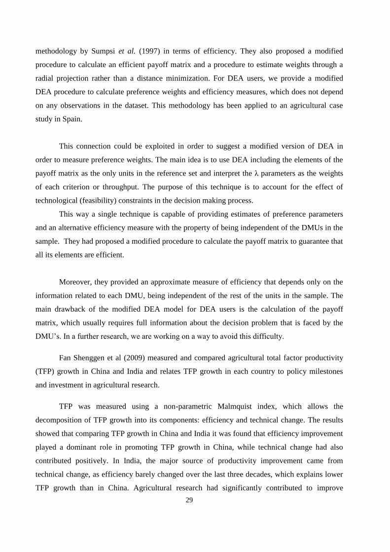
The per capita availability of surface water in Tamil Nadu has come down from 803 cubic
meter in 1951 to 389 cubic meter in 2001(Table 5.). This is mainly due to population explosion
and increase in usage of water in industrial sector.
Table 6.Seasonwise Rainfall in Tamil Nadu (mm)
Year Southwest Northeast Winter Summer Total Rainfall
1979-80 196.4 337.0 10.5 125.4 669.3
1989-90 348.8 341.0 90.2 136.7 916.7
1999-2000 199.9 499.5 119.5 77.9 896.8
2007-08 341.6 515.4 46.2 261.2 1164.4
The state‟s annual normal rainfall is 958.51mm. Nearly more than 30% of the crops
grown in the state are under rainfed condition.
From the table it is evidenced that variation in rainfall received was higher and more than
40% of the rainfall was received from Northeast monsoon period. With the total rainfall of
1164.4 mm received during 2007-08, it was rated as 'excess' and emerged to be more beneficial
to cropping.
Table 7. Irrigation Status in Tamil Nadu (Area in lakh ha)
Particulars 1989-90 1999-2000 2006-07
Gross Irrigated Area 30.4 35.9 33.1
Net Irrigated Area 24.9 29.7 28.9
Canals 7.9 8.7 7.8
Tanks 5.2 6.3 5.3
Wells 11.7 14.5 15.7
Others 0.1 0.1 0.1
Area Irrigated More than Once 5.5 6.2 4.2

39
The age old structures, inadequate maintenance, encroachment in the catchments and
foreshore areas, large scale siltation, the live practice of fragmentation of holdings, lack of
institutional arrangements for the supply of water, widespread deviations from the intended
cropping pattern, seepage, percolation, evaporation, diversion of ayacut for nonagricultural
purposes, excessive drawal in the upper reaches, unauthorized drawal etc. have caused a wide
gap between the potential created and its utilization in the case of surface flow sources of
irrigation in the State.
The net area irrigated by surface flow source has become stagnant as 13.1 lakh hectares in
1989-90 and in 2006-07(Table 7.). Due to the proliferation of wells, the extent of area irrigated
increased from 11.7 in 1989-90 to 15.7 lakh hectares in 2006-07, increasing its relative share in
the total net area irrigated in the State from 24 to 54 percent. Proliferation of wells and
indiscriminate drawal of water has its own adverse effect on the water table. Due to this area
irrigated more than once has come down from 5.5 lakh ha in 1989-90 to 4.2 lakh ha in 2006-07.
Viewed against these serious limitations, the overall irrigation scenario in the State is
uninspiring.
At this juncture, even to maintain the existing irrigated area, the State has to focus its
attention on popularization and adoption of water saving techniques which saves 40-70 per cent
of water as compared to field irrigation, bringing in atleast 10 per cent of the total irrigated area
under these techniques, popularization of rainwater harvesting and conservation techniques,
evolving an integrated approach to use surface and groundwater conjunctively, equipping and
involving the farmers in the maintenance of source and water distribution, regularizing the
drawal of groundwater with the safe limits and minimization of water losses.
Table 8.Change in Availability of Groundwater in Tamil Nadu
S.No Year of
Assessment
No. of
Districts
Total
No. of
Blocks
Categorization of Blocks
Dark (85 – 100%) Grey (65 – 85%) White
(65%)
1 1987 19 378 41 86 251
2 1992 22 384 89 86 209
Over
Exploited
(>100%)
Critical
(90 –
100%)
Semi
Critical
(70-
90%)
Safe
(<70%)
Saline
3 1998 28 385 135 35 70 137 8
4 2003 28 385 135 37 105 97 8
Source: Water Resource Organisation, Govt. of Tamil Nadu.

40
As per the latest estimates of January 2003, the State has tapped 86 percent of
groundwater potential. Across the State, the untapped groundwater potential is distributed in 97
safe blocks (tapping of potential <70%), 105 semi-critical blocks (>70% to<90%) and183 critical
blocks (>90% to<100%). In about 138 blocks (36% of the total blocks in the State), the potential
has been over exploited, exceeding the recharge capacity (Table 8.). As a result, the number of
dark blocks is increasing.
5.3. Problems facing Agriculture in the State
5.3.1. Land degradation and soil quality
Crop yields are dependent on certain soil characteristics- soil nutrient content, water-
holding capacity, organic matter content, acidity, top soil depth and soil biomass and so on. Soil
erosion is by wind or water. Erosion causes depletion of fertility through the removal of the
valuable and fertile surface soil. In Tamil Nadu, erosion is observed in and around 13 lakh ha.
The organic matter content in the soil has gone down from 1.20% in 1971 to 0.68% in 2002 in
Tamil Nadu, because of less use of organic inputs.
5.3.2. Wastelands
The adverse effect of salinity in soil is that it hinders crop growth and results in reduction
in crop yield. The estimated extent of soils affected by salinity and alkalinity is estimated at 2.48
L.ha. Besides 1.23 L.ha. Suffering from acidic soils. Excess water hinders plant growth by
reducing aeration, which in turn decreases the water absorption and nutrient uptake by roots.
The coastal regions of Tamil Nadu face heavy damages due to water logging. The
command areas in major irrigation projects experience water logging problem. In Tamil Nadu
44,820 ha is estimated as marshy lands. About 14 percent of the area in Tamil Nadu is under very
poorly drained soils. Another 16 percent is under moderately well drained to well drain soils and
15 percent is somewhat excessively drained soil.
The gullies are the first stage of excessive land dissection followed by their networking
which lead to the development of ravine land. The ravines are extensive system of gullies
developed along nullas, streams, and river coarse. It has been estimated that Tamil Nadu has
22,550 ha. Under gullied / ravine lands. Wastelands are degraded lands that can be brought under
vegetative cover.
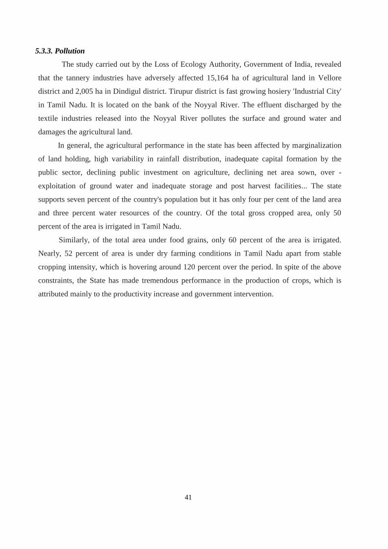
41
5.3.3. Pollution
The study carried out by the Loss of Ecology Authority, Government of India, revealed
that the tannery industries have adversely affected 15,164 ha of agricultural land in Vellore
district and 2,005 ha in Dindigul district. Tirupur district is fast growing hosiery 'Industrial City'
in Tamil Nadu. It is located on the bank of the Noyyal River. The effluent discharged by the
textile industries released into the Noyyal River pollutes the surface and ground water and
damages the agricultural land.
In general, the agricultural performance in the state has been affected by marginalization
of land holding, high variability in rainfall distribution, inadequate capital formation by the
public sector, declining public investment on agriculture, declining net area sown, over -
exploitation of ground water and inadequate storage and post harvest facilities... The state
supports seven percent of the country's population but it has only four per cent of the land area
and three percent water resources of the country. Of the total gross cropped area, only 50
percent of the area is irrigated in Tamil Nadu.
Similarly, of the total area under food grains, only 60 percent of the area is irrigated.
Nearly, 52 percent of area is under dry farming conditions in Tamil Nadu apart from stable
cropping intensity, which is hovering around 120 percent over the period. In spite of the above
constraints, the State has made tremendous performance in the production of crops, which is
attributed mainly to the productivity increase and government intervention.
42
CHAPTER VI
Profile of River Basins of Tamil Nadu
6. Profile of River Basins of Tamil Nadu
The river basins in Tamil Nadu are grouped into 17 major river basins as furnished below.
Figure 2. River Basins of Tamil Nadu
Table 9.Major River Basins of Tamil Nadu
Name of the Major River Basin Group River Basins in the Group
1. Chennai Basin Group 1. Araniyar
2. Kusaithalaiyar
3. Cooum
4. Adayar
2. Palar 5. Palar
3. Varahanadhi 6. Ongur
7. Varahanadhi
4. Ponnaiyaar 8. Malattar
9. Ponnaiyaar
10. Gadilam
5. Vellar 11. Vellar

43
6. Paravanar
7. Cauvery 12. Cauvery
8. Agniyar 13. Agniyar
14. Ambuliyar
15. Vellar
9. Pambar and
Kottakaraiyar
16. Koluvanar
17. Pambar
18. Manimukthar
19. Kottakaraiyar
10. Vaigai 20. Vaigai
11. Gundar 21. Uthirakosamangaiyar
22. Gundar
23. Vembar
12. Vaippar 24. Vaippar
13. Kallar . 25.Kallar
2 26. Korampallam Aru
14. Thambaraparani 27. Thambaraparani
15. Nambiyar 28. Karmaniar
29. Nambiyar
30. Hanumanadhi
16. Kodaiyar 31. Palayar
32. Valliyar
33. Kodaiyar
17. PAP 34.West flowing river
Table 10.Area and Rainfall of the River Basins
S.No Name of the Major
River Basin Group
Area of
the basin
(sq.km)
Normal
Annual
Rainfall
(mm)
Normal Rain
Volume
(Km3)
System
tanks
Non
system
tanks
1. Chennai Basin Group 5542 1130 6.26 1304 215
2. Palar 10911 940 10.03 661
3. Varahanadhi 4214 1250 4.55 131 1290
4. Ponnaiyar 11257 920 11.17 1133
5. Vellar 7659 980 386 71
6. Paravanar 760 8.39 2 9
7. Cauvery 43867 930 45.32
8. Agniyar 4566 910 4.06 346 3629
9. Pambar and
Kottakaraiyar 5847 880 3.07 160 1161
10. Vaigai 7031 900 6.97 521 976
11. Gundar 5647 770 3.73 526 123
12. Vaippar 5423 800 5.00 151 711
13. Kallar 1879 600 1.04 15 184
14. Thambaraparani 5969 1110 6.09 1300
15. Nambiyar 2084 950 1.48 559 38
16. Kodaiyar 1533 1720 2.64 2 1460
17. PAP 3462 610 1.33

44
Table 11.Surface and Groundwater Potential (MCM) of the River Basins
S.No Name of the Major
River Basin Group
Surface water
potential
Groundwater
potential
Other
sources
Total water
potential
1. Chennai Basin Group 906.00 1120.22 2026.22
2. Palar 1758.00 2610.32 4368.32
3. Varahanadhi 412.09 1482.07 4.00 1898.16
4. Ponnaiyaar 1310.43 1560.00 2870.43
5. Vellar 1065.00 1344.00 6.00 2415.00
6. Paravanar 104.30 225.50 39.70 370.00
7. Cauvery 5962.00 2869.00 8831.00
8. Agniyar 585.00 920.00 499.00 2004.00
9. Pambar and
Kottakaraiyar
653.00 976.00 1629.00
10. Vaigai 1579.00 993.00 2572.00
11. Gundar 567.52 766.00 1334.00
12. Vaippar 611.00 1167.00 4.82 1782.82
13. Kallar 124.56 69.58 17.37 211.51
14. Thambaraparani 1375.00 744.00 2119.00
15. Nambiyar 203.87 274.74 478.61
16. Kodaiyar 925.00 342.10 1267.10
17. PAP 416.00 751.001 1167.00
Detailed particulars of the each river basin such as basin area, districts in which they fall, sub-
basins etc are provided in Appendix-I

45
CHAPTER VII
Methodology
7. Methodology
The proposed methodology to study the total factor productivity (TFP) of agriculture in
river basins of Tamil Nadu consists of the following three steps:
7.1. Estimation of basin areas and proportion of basin areas in each district of Tamil Nadu:
Estimates of 17 river basin areas are available from published records. Also rough
estimates of area of each basin in each district are available and these figures must be checked for
their accuracy. This will be done by using GIS techniques and the figures will be revised. Using
these figures, the proportion of area occupied by each basin in each district will be estimated.
7.2. Conversion of district-wise data to basin-wise:
Data on various input and output variables are available district wise from published
records. Further, these districts, which were 24 in number during 1970s have been subdivided
over years and now there are 31 districts and recent data are available only for the new districts
while figures for past years are available only for the original districts.
So first, these data will be aggregated either to the original districts or for the latest
districts. Apportion these revised time series figures will be then to various basins based on the
estimates obtained in Step 1 as follows: Let DjBipij ,...2,1;,...2,1 be the proportion of area
occupied by basin i in district j and B and D be respectively the total number of basins and
districts. Also let xd be the value of a input or output variable for the district d in a certain year
and yb be the estimated value of that variable for basin b during the same year. Also let
1 1 11 12 1
2 2 21 22 2
1 2
and
D
D
B D B B BD
y x p p . . p
y x p p . . p
Y X P. . . . . . .
. . . . . . .
y x p p . . p
It can be easily checked that
Y PX
The above formula provides an elegant method of estimation of figures for each basin.
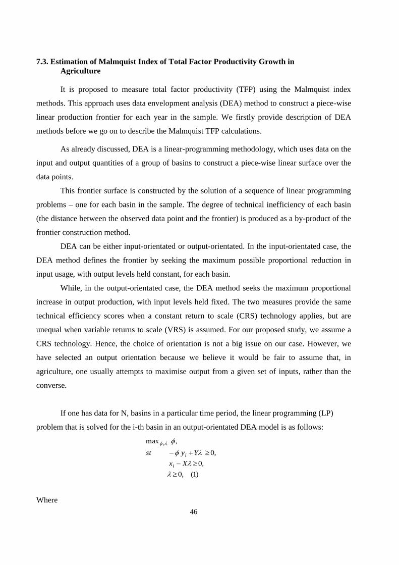
46
7.3. Estimation of Malmquist Index of Total Factor Productivity Growth in
Agriculture
It is proposed to measure total factor productivity (TFP) using the Malmquist index
methods. This approach uses data envelopment analysis (DEA) method to construct a piece-wise
linear production frontier for each year in the sample. We firstly provide description of DEA
methods before we go on to describe the Malmquist TFP calculations.
As already discussed, DEA is a linear-programming methodology, which uses data on the
input and output quantities of a group of basins to construct a piece-wise linear surface over the
data points.
This frontier surface is constructed by the solution of a sequence of linear programming
problems – one for each basin in the sample. The degree of technical inefficiency of each basin
(the distance between the observed data point and the frontier) is produced as a by-product of the
frontier construction method.
DEA can be either input-orientated or output-orientated. In the input-orientated case, the
DEA method defines the frontier by seeking the maximum possible proportional reduction in
input usage, with output levels held constant, for each basin.
While, in the output-orientated case, the DEA method seeks the maximum proportional
increase in output production, with input levels held fixed. The two measures provide the same
technical efficiency scores when a constant return to scale (CRS) technology applies, but are
unequal when variable returns to scale (VRS) is assumed. For our proposed study, we assume a
CRS technology. Hence, the choice of orientation is not a big issue on our case. However, we
have selected an output orientation because we believe it would be fair to assume that, in
agriculture, one usually attempts to maximise output from a given set of inputs, rather than the
converse.
If one has data for N, basins in a particular time period, the linear programming (LP)
problem that is solved for the i-th basin in an output-orientated DEA model is as follows:
)1(,0
,0
,0
,max ,
Xx
Yyst
i
i
Where

47
iy is a Mx1 vector of output quantities for the i-th basin;
ix is a Kx1 vector of input quantities for the i-th basin;
Y is a NxM matrix of output quantities for all N basins;
X is a NxK matrix of input quantities for all N basins;
is a Nx1 vector of weights; and
is as scalar.
It must be noted that the parameter will take a value greater than or equal to one, and that -1
is the proportional increase in outputs that could be achieved by the i-th basin, with input
quantities held constant. Note also that 1/ defines a technical efficiency (TE) score with varies
between zero and one.
The above LP is solved B times – once for each basin in the sample. Each LP produces a
and a vector. The -parameter – provides information on the technical efficiency score for
the i-th basin the -vector provides information on the peers of the (inefficient) i-th basin. The
peers of the i-th basin are those efficient that define the facet of the frontier against which the
(inefficient) i-th basin is projected.
7.4. The Malmquist TFP Index
The Malmquist index is defined using distance functions. Distance functions allow one to
describe a multi-input, multi-output production technology without the need to specify a
behavioural objective (such as cost minimization or profit maximization). One may define input
distance functions and output distance functions. An input distance function characterizes the
production technology by looking at a minimal proportional contraction of the input vector, given
an output vector. An output distance function considers a maximal proportional expansion of the
output vector, given an input vector. We only consider an output distance function in detail in
this paper. However, input distance functions can be defined and used in a similar manner.
A production technology may be defined using the output set, P(x), which represents the
set of all output vectors, y, which can be produced using the input vector, x. That is,
.producecan:)( yxyxP
The output distance function is defined on the output set, P (x), as:
.)(/:min, xPyyxdo
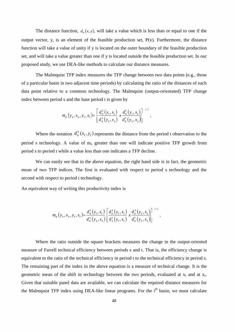
48
The distance function, yxdo , , will take a value which is less than or equal to one if the
output vector, y, is an element of the feasible production set, P(x). Furthermore, the distance
function will take a value of unity if y is located on the outer boundary of the feasible production
set, and will take a value greater than one if y is located outside the feasible production set. In our
proposed study, we use DEA-like methods to calculate our distance measures.
The Malmquist TFP index measures the TFP change between two data points (e.g., those
of a particular basin in two adjacent time periods) by calculating the ratio of the distances of each
data point relative to a common technology. The Malmquist (output-orientated) TFP change
index between period s and the base period t is given by
,
,
,
,
,,,,
2/1
ssto
ttto
ssso
ttso
ttssoxyd
xydx
xyd
xydxyxym
Where the notation ),( ttso yxd represents the distance from the period t observation to the
period s technology. A value of mo greater than one will indicate positive TFP growth from
period s to period t while a value less than one indicates a TFP decline.
We can easily see that in the above equation, the right hand side is in fact, the geometric
mean of two TFP indices. The first is evaluated with respect to period s technology and the
second with respect to period t technology.
An equivalent way of writing this productivity index is
,
,
,
,
,
,
,,,,
2/1
ssto
ssso
ttto
ttso
ssso
ttto
ttssoxyd
xydx
xyd
xyd
xyd
xydxyxym
Where the ratio outside the square brackets measures the change in the output-oriented
measure of Farrell technical efficiency between periods s and t. That is, the efficiency change is
equivalent to the ratio of the technical efficiency in period t to the technical efficiency in period s.
The remaining part of the index in the above equation is a measure of technical change. It is the
geometric mean of the shift in technology between the two periods, evaluated at xt and at xs.
Given that suitable panel data are available, we can calculate the required distance measures for
the Malmquist TFP index using DEA-like linear programs. For the ith
basin, we must calculate
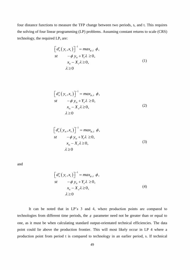
49
four distance functions to measure the TFP change between two periods, s, and t. This requires
the solving of four linear programming (LP) problems. Assuming constant returns to scale (CRS)
technology, the required LPs are:
1
0
0
0
t
o t t ,
it t
it t
d y ,x max ,
st y Y ,
x X ,
(1)
1
0
0
0
s
o s s ,
is s
is s
d y ,x max ,
st y Y ,
x X ,
(2)
1
0
0
0
t
o st s ,
is t
is t
d y ,x max ,
st y Y ,
x X ,
(3)
and
1
0
0
0
s
o t t ,
it s
it s
d y ,x max ,
st y Y ,
x X ,
(4)
It can be noted that in LP‟s 3 and 4, where production points are compared to
technologies from different time periods, the parameter need not be greater than or equal to
one, as it must be when calculating standard output-orientated technical efficiencies. The data
point could lie above the production frontier. This will most likely occur in LP 4 where a
production point from period t is compared to technology in an earlier period, s. If technical

50
progress has occurred, then a value of <1 is possible. It could also possibly occur in LP 3 if
technical regress has occurred, but this is less likely.
In the input-orientated case, the DEA defines the frontier by seeking the maximum
possible proportional reduction in input usage, with output levels held constant, for each River
Basin. In the output-orientated case, DEA seeks the maximum proportional increase in output
production, with input levels held fixed. The two measures provide the same technical efficiency
scores when a constant return to scale (CRS) technology applies.
In this study, we select an output orientation with assumption of CRS. Because, in
agriculture, one usually attempts to maximize output from a given set of inputs, rather than
minimizing the inputs for a given level of output.
Therefore, we are assuming constant returns to scale technology for this analysis. The
Malmquist total factor productivity change indices are decomposed into technical change and
technical efficiency change components. The above approach is further extended by
decomposing technical efficiency change into scale efficiency and pure technical efficiency
components.
As the proposed study is of empirical in nature and the study is intended to utilize both
primary and secondary data for past 30 years from published and unpublished records.
Secondary sources for data collection were Seasons and Crop Report, Economic Appraisal of
Tamil Nadu, Statistics at a Glance, Publications of Central Water Commission, Published, and
unpublished records of Public Works Department, Census of India, Livestock Census, District
Statistical Office, and Department of Agriculture etc.
51
CHAPTER VIII
Basin coverage and Time Period
The data for the present study consisted of the following:
8. Basin coverage: All the river basins of Tamil Nadu were included in the present study. They
were Chennai basin, Palar basin, Varahanadhi basin, Ponnaiyaar basin, Vellar basin, Paravanar
basin, Cauvery basin, Agniyar basin, Pambar and Kottakaraiyar basin, Vaigai basin, Gundar
basin, Vaippar basin, Kallar basin, Thambaraparani basin, Nambiar basin, Kodaiyar basin and
Parambikulam Azhiyar Project (PAP) basin
8.1. Time period: the study covers the period of 1975 -76 and 2005 -2006, which concerned with
important changes in agriculture due to liberalization of trade and reforms in investment,
initiation of privatization, tax reforms and inflation controlling measures.
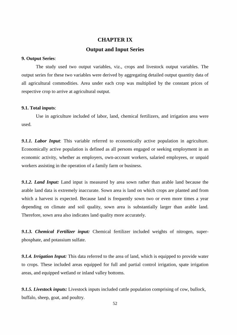
52
CHAPTER IX
Output and Input Series
9. Output Series:
The study used two output variables, viz., crops and livestock output variables. The
output series for these two variables were derived by aggregating detailed output quantity data of
all agricultural commodities. Area under each crop was multiplied by the constant prices of
respective crop to arrive at agricultural output.
9.1. Total inputs:
Use in agriculture included of labor, land, chemical fertilizers, and irrigation area were
used.
9.1.1. Labor Input: This variable referred to economically active population in agriculture.
Economically active population is defined as all persons engaged or seeking employment in an
economic activity, whether as employers, own-account workers, salaried employees, or unpaid
workers assisting in the operation of a family farm or business.
9.1.2. Land Input: Land input is measured by area sown rather than arable land because the
arable land data is extremely inaccurate. Sown area is land on which crops are planted and from
which a harvest is expected. Because land is frequently sown two or even more times a year
depending on climate and soil quality, sown area is substantially larger than arable land.
Therefore, sown area also indicates land quality more accurately.
9.1.3. Chemical Fertilizer input: Chemical fertilizer included weights of nitrogen, super-
phosphate, and potassium sulfate.
9.1.4. Irrigation Input: This data referred to the area of land, which is equipped to provide water
to crops. These included areas equipped for full and partial control irrigation, spate irrigation
areas, and equipped wetland or inland valley bottoms.
9.1.5. Livestock inputs: Livestock inputs included cattle population comprising of cow, bullock,
buffalo, sheep, goat, and poultry.

53
9.1.6. Units of variables: The table below provides the units of various variables used in the
present study.
Variable Unit
Agricultural output Rupees in Crores Net sown area hectare
Crop output Rupees in Crores
Net Irrigated area hectare
Livestock output Rupees in Crores
NPK consumption lakh tones
Labour input Numbers
Cattle and poultry numbers

54
CHAPTER X
Results and Discussions
10. Results and Discussions
10.1. Summary Statistics
10.1.1. Crop output
The summary statistics of output and input variables namely crop output, livestock
output, net sown area, net irrigated area, NPK intake, labour input, cattle input and poultry input
for all the basins are presented and discussed below.
Table 12.Summary Statistics Crop output (Rs.Crores)
Sl.No Name of the basin Area of the
basin Max Min Average SD CV (%)
1 Chennai Basin 5542 2002 113 822 669 81
2 Palar River Basin 10911 5537 320 2041 1697 83
3 Varahanadhi River Basin 4214 3850 134 1392 1289 93
4 Ponnaiyaar River Basin 11257 11553 374 2928 2614 89
5 Paravanar River Basin 7659 830 25 294 282 96
6 Vellar Basin 760 8737 280 2329 2091 90
7 Cauvery River Basin 43867 24550 1934 7435 5750 77
8 Agniyar River Basin 4566 2494 74 547 564 103
9
Pambar & Kottakaraiyar
River Basin
5847
1204 103 434 315 73
10 Vaigai River Basin 7031 3169 221 1001 766 77
11 Gundar River Basin 5647 1600 133 537 380 71
12 Vaippar Basin 5423 1045 96 445 280 63
13 Kallar River Basin 1879 137 31 85 33 39
14 Thambaraparani River Basin 5969 883 77 374 241 64
15 Nambiyar River Basin 2084 281 28 125 75 60
16 Kodaiyar River Basin 1533 757 10 106 130 123
17 P.A.P. Basin 3462 1589 246 596 321 54
From the above table it could be noted that there was wide range of crop output in all the
river basins. The coefficient of variation was more than fifty percent in general and it was more
than hundred in Agniyar and Kodaiyar river basin. The minimum value was less than hundred
crores in river basins namely Paravanar, Agniyar, Vaippar, Kallar, Thambaraparani, Nambiar,
and Kodaiyar. The crop output depended on the value of the crop and its area. For comparing the
crop output, the basins were classified as small, medium, and large depending on net sown area.
The following figures provide the performance of the basins in the three categories over the
period 1975-76 to 2005-06.
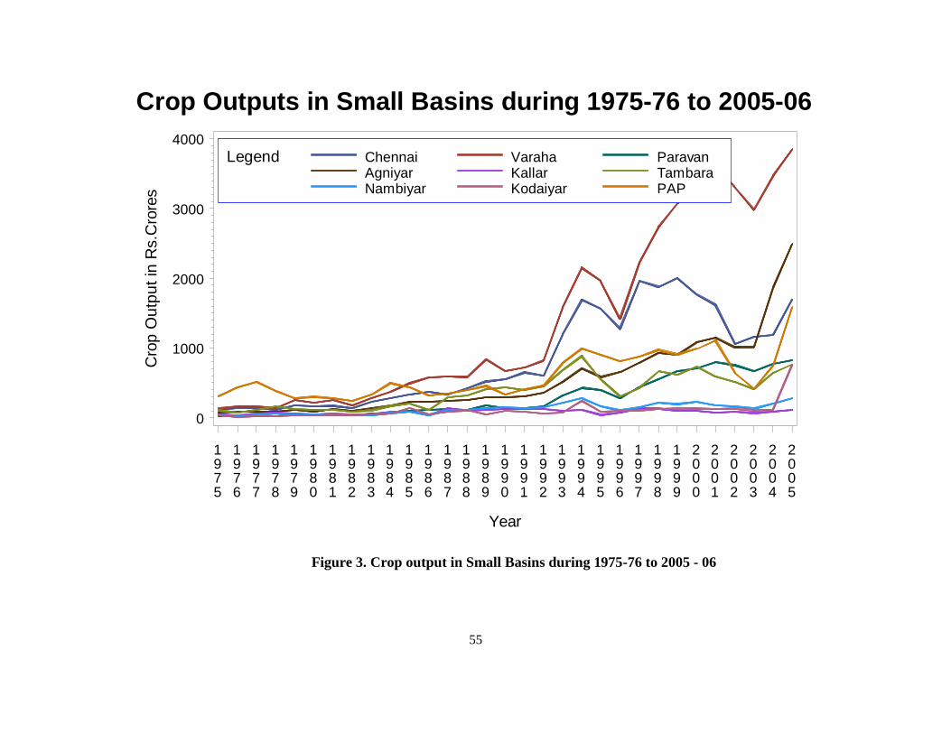
55
Cro
p O
utp
ut
in R
s.C
rore
s
0
1000
2000
3000
4000
Year
1975
1976
1977
1978
1979
1980
1981
1982
1983
1984
1985
1986
1987
1988
1989
1990
1991
1992
1993
1994
1995
1996
1997
1998
1999
2000
2001
2002
2003
2004
2005
Crop Outputs in Small Basins during 1975-76 to 2005-06
Legend Chennai Varaha ParavanAgniyar Kallar TambaraNambiyar Kodaiyar PAP
Figure 3. Crop output in Small Basins during 1975-76 to 2005 - 06

56
Cro
p O
utp
ut
in R
s.C
rore
s
0
1000
2000
3000
4000
5000
6000
7000
8000
9000
Year
1975
1976
1977
1978
1979
1980
1981
1982
1983
1984
1985
1986
1987
1988
1989
1990
1991
1992
1993
1994
1995
1996
1997
1998
1999
2000
2001
2002
2003
2004
2005
Crop Outputs in Medium Basins during 1975-76 to 2005-06
Legend Vellar Pambar VaigaiGundar Vaippar
Figure 4. Crop output in Medium Basins during 1975-76 to 2005 – 06
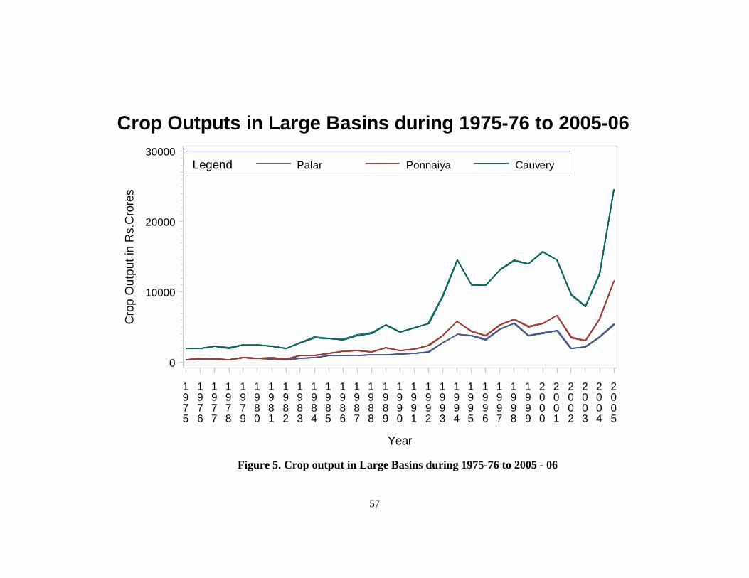
57
Cro
p O
utp
ut
in R
s.C
rore
s
0
10000
20000
30000
Year
1975
1976
1977
1978
1979
1980
1981
1982
1983
1984
1985
1986
1987
1988
1989
1990
1991
1992
1993
1994
1995
1996
1997
1998
1999
2000
2001
2002
2003
2004
2005
Crop Outputs in Large Basins during 1975-76 to 2005-06
Legend Palar Ponnaiya Cauvery
Figure 5. Crop output in Large Basins during 1975-76 to 2005 - 06

58
From the graphs, it could be seen that among the small basins, Varahanadhi Basin ranks
first in terms of crop output during the last five years, 2001-02 to 2005-06. Among the medium
basins, Vellar basin ranks first and Cauvery basin ranks first consistently among the large basins
10.1.2. Livestock output
The table below provides a summary of livestock output in all the basins. Livestock is
one of the major allied activities of agriculture. Highest value of livestock output was recorded in
Cauvery basin followed by Ponnaiyaar and Vellar basins. The coefficient of variation was
hundred and less than hundred. Comparing base year i.e. 1976 there was increase in livestock
population in all the basins. This was mainly due to sustained income from livestock and in most
of the farms, livestock was maintained by family labour they.
Table 13.Summary Statistics - Livestock output (Rs.Crores)
S.No Name of the basin Max Min Average SD CV (%)
1 Chennai Basin 402 11 136 132 97
2 Palar River Basin 570 27 251 197 79
3 Varahanadhi River Basin 196 8 79 67 85
4 Ponnaiyaar River Basin 663 17 210 183 87
5 Paravanar River Basin 31 1 11 11 100
6 Vellar Basin 593 17 190 169 89
7 Cauvery River Basin 2569 102 934 740 79
8 Agniyar River Basin 223 7 78 72 92
9 Pambar & Kottakaraiyar River Basin 164 7 68 55 80
10 Vaigai River Basin 324 10 127 103 81
11 Gundar River Basin 200 7 79 66 83
12 Vaippar Basin 223 5 62 64 103
13 Kallar River Basin 105 4 28 26 94
14 Tambarabarani River Basin 281 7 70 73 104
15 Nambiyar River Basin 104 3 27 27 99
16 Kodaiyar River Basin 115 6 42 36 86
17 P.A.P. Basin 171 6 67 51 76

59
10.1.3. Net Sown Area and net irrigated area
The next two tables provide a summary of net sown area in all the 17 basins. Though net
irrigated area increased over the decades, there was not much increase in net sown area. This was
supported by the minimum of coefficient of variation as given in the table.
It was evidenced from Tamil Nadu state data on net sown area. Average net sown area in
the decade 1980-90 was 56.22 lakh ha and it was reduced to 50.62 lakh ha in the year 2007-08.
Land put to non-agricultural purposes has increased from 16 lakh ha in 1970s to 21.61 lakh ha in
2007-08. Other fallow lands have increased from 5.31 lakh ha in 1970s to 14.99 lakh ha in 2007-
08. There was considerable increase in net irrigated area in all river basins over three decades.
The coefficient of variation was in the range of 27 to 38 percentages. This was mainly due to
development of groundwater irrigation. As per the latest estimates of January 2003, the State has
tapped 86 percent of groundwater potential. This statement was well supplement by the statistics
of increase in area under well-irrigated area from 11.7 lakh ha (1989-90) to 15.7 lakh.ha in 2006-
07 in Tamil Nadu state.
Table 14.Summary Statistics - Net-Area-Sown-Input (Area in ha)
S.No Name of the basin Max Min Average SD CV
1 Chennai Basin 249108 150179 206499 25086 12
2 Palar River Basin 533525 306677 451031 51629 11
3 Varahanadhi River Basin 188903 143563 174477 11447 7
4 Ponnaiyaar River Basin 721218 539594 659571 49727 8
5 Paravanar River Basin 33585 25429 31030 1787 6
6 Vellar Basin 412352 314088 381649 25502 7
7 Cauvery River Basin 2046556 1644539 1907825 97386 5
8 Agniyar River Basin 249301 143965 205154 25491 12
9
Pambar & Kottakaraiyar
River Basin 253484 188930 220498 16560 8
10 Vaigai River Basin 344108 200851 277800 43811 16
11 Gundar River Basin 287527 207989 247578 23012 9
12 Vaippar Basin 280109 159031 217028 38600 18
13 Kallar River Basin 132971 63890 95403 21046 22
14 Tambarabarani River Basin 169148 118493 145162 13710 9
15 Nambiyar River Basin 75692 51010 62284 6719 11
16 Kodaiyar River Basin 81431 73000 77040 2333 3
17 P.A.P. Basin 172086 133868 153051 10095 7

60
Table 15.Summary Statistics - Net Irrigated Area Input (Area in ha)
S.No Name of the basin Max Min Average SD CV (%)
1 Chennai Basin 426456 133033 305920 97650 32
2 Palar River Basin 764884 202507 500127 171061 34
3 Varahanadhi River Basin 328864 80755 221957 70637 32
4 Ponnaiyaar River Basin 702206 161364 483752 176411 36
5 Paravanar River Basin 69643 12770 37270 12864 35
6 Vellar Basin 497413 130095 359684 124561 35
7 Cauvery River Basin 2499734 742220 1799856 595109 33
8 Agniyar River Basin 314983 120042 234890 69022 29
9 Pambar & Kottakaraiyar 266309 110143 204078 54700 27
10 Vaigai River Basin 350523 117251 258421 81892 32
11 Gundar River Basin 228040 92306 175828 47825 27
12 Vaippar Basin 168546 77505 128190 29441 23
13 Kallar River Basin 47870 16319 32647 9041 28
14 Thambaraparani River Basin 240706 74035 172689 56148 33
15 Nambiyar River Basin 79369 25108 57108 18276 32
16 Kodaiyar River Basin 77438 24681 55850 21005 38
17 P.A.P. Basin 172437 48208 124819 39585 32
10.1.4. Fertilizer Usage: Fertilizer was a major input for agriculture in Tamil Nadu. The relevant
summary statistics are presented in the table below:
Table 16.Summary Statistics - NPK-Value-Input (in lakh tonnes)
S.No Name of the basin Max Min Average SD CV (%)
1 Chennai Basin 0.65 0.15 0.41 0.11 26.68
2 Palar River Basin 1.25 0.29 0.72 0.21 29.41
3 Varahanadhi River Basin 0.57 0.18 0.40 0.10 25.26
4 Ponnaiyar River Basin 0.91 0.11 0.45 0.25 56.00
5 Paravanar River Basin 0.12 0.04 0.08 0.02 27.75
6 Vellar Basin 1.17 0.22 0.61 0.22 35.92
7 Cauvery River Basin 4.16 0.92 2.65 0.75 28.08
8 Agniyar River Basin 0.92 0.13 0.40 0.18 44.05
9 Pambar & Kottakaraiyar 1.01 0.12 0.25 0.17 68.42
10 Vaigai River Basin 0.85 0.17 0.43 0.14 32.57
11 Gundar River Basin 0.44 0.12 0.25 0.08 31.06
12 Vaippar Basin 0.28 0.09 0.17 0.05 29.10
13 Kallar River Basin 0.10 0.02 0.05 0.02 29.43
14 Tambarabarani River Basin 0.37 0.10 0.26 0.07 28.76
15 Nambiyar River Basin 0.12 0.04 0.09 0.02 25.37
16 Kodaiyar River Basin 0.20 0.04 0.11 0.04 36.15
17 P.A.P. Basin 0.34 0.07 0.23 0.06 26.38

61
It could be seen from the above table that there was considerable increase in intake of
NPK fertilizers in all river basins. As the decades under consideration were after green
revolution, the intake of inorganic fertilizers had increased due to increase in area under high
yielding varieties and area under irrigation.
10.1.5. Labour input
Labour was a major input. Table below summarizes the usage of labour in all the river
basins. Even though the quantum of usage varied widely across the basins, the coefficient of
variation for this input ranged between 6 and 33 percentages between the basins.
Table 17.Summary Statistics - Labour input (in Numbers)
S.No Name of the basin Max Min Average SD CV (%)
1 Chennai Basin 389181 261467 352125 46606 13
2 Palar River Basin 826761 506993 700631 104779 15
3 Varahanadhi River Basin 370331 185093 278078 58660 21
4 Ponnaiyaar River Basin 1077715 473443 765766 191128 25
5 Paravanar River Basin 68385 30956 48521 11769 24
6 Vellar Basin 784325 339241 537435 139010 26
7 Cauvery River Basin 3399740 1523559 2325241 567675 24
8 Agniyar River Basin 381088 131609 233214 77546 33
9 Pambar & Kottakaraiyar 276366 119130 197850 51409 26
10 Vaigai River Basin 537372 345827 475144 73805 16
11 Gundar River Basin 305872 202382 270506 37524 14
12 Vaippar Basin 280242 207580 242889 21031 9
13 Kallar River Basin 80968 58671 70333 6504 9
14 Thambaraparani River Basin 293731 218184 271100 26981 10
15 Nambiyar River Basin 105739 79115 95293 7960 8
16 Kodaiyar River Basin 166546 33227 121133 38121 31
17 P.A.P. Basin 207306 164241 192357 10585 6
10.1.6. Cattle and poultry input
There was tremendous increase in poultry population in Tamil Nadu especially in
Cauvery basin and P.A.P basin. Poultry is the perfect substitute for meat. Low price and
adequate supply were main reason for development of poultry as commercial venture in this
area. Weather and technical expertise were reasons for concentration of poultry units in these
two basins.
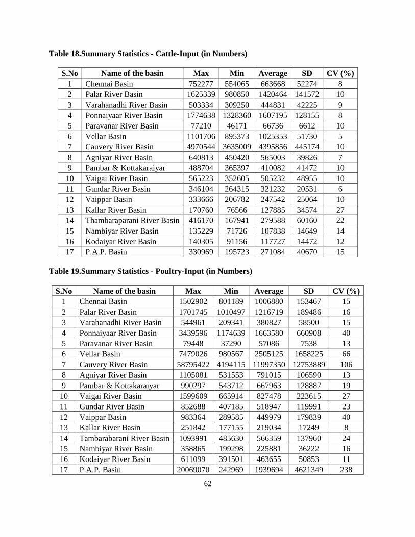
62
Table 18.Summary Statistics - Cattle-Input (in Numbers)
S.No Name of the basin Max Min Average SD CV (%)
1 Chennai Basin 752277 554065 663668 52274 8
2 Palar River Basin 1625339 980850 1420464 141572 10
3 Varahanadhi River Basin 503334 309250 444831 42225 9
4 Ponnaiyaar River Basin 1774638 1328360 1607195 128155 8
5 Paravanar River Basin 77210 46171 66736 6612 10
6 Vellar Basin 1101706 895373 1025353 51730 5
7 Cauvery River Basin 4970544 3635009 4395856 445174 10
8 Agniyar River Basin 640813 450420 565003 39826 7
9 Pambar & Kottakaraiyar 488704 365397 410082 41472 10
10 Vaigai River Basin 565223 352605 505232 48955 10
11 Gundar River Basin 346104 264315 321232 20531 6
12 Vaippar Basin 333666 206782 247542 25064 10
13 Kallar River Basin 170760 76566 127885 34574 27
14 Thambaraparani River Basin 416170 167941 279588 60160 22
15 Nambiyar River Basin 135229 71726 107838 14649 14
16 Kodaiyar River Basin 140305 91156 117727 14472 12
17 P.A.P. Basin 330969 195723 271084 40670 15
Table 19.Summary Statistics - Poultry-Input (in Numbers)
S.No Name of the basin Max Min Average SD CV (%)
1 Chennai Basin 1502902 801189 1006880 153467 15
2 Palar River Basin 1701745 1010497 1216719 189486 16
3 Varahanadhi River Basin 544961 209341 380827 58500 15
4 Ponnaiyaar River Basin 3439596 1174639 1663580 660908 40
5 Paravanar River Basin 79448 37290 57086 7538 13
6 Vellar Basin 7479026 980567 2505125 1658225 66
7 Cauvery River Basin 58795422 4194115 11997350 12753889 106
8 Agniyar River Basin 1105081 531553 791015 106590 13
9 Pambar & Kottakaraiyar 990297 543712 667963 128887 19
10 Vaigai River Basin 1599609 665914 827478 223615 27
11 Gundar River Basin 852688 407185 518947 119991 23
12 Vaippar Basin 983364 289585 449979 179839 40
13 Kallar River Basin 251842 177155 219034 17249 8
14 Tambarabarani River Basin 1093991 485630 566359 137960 24
15 Nambiyar River Basin 358865 199298 225881 36222 16
16 Kodaiyar River Basin 611099 391501 463655 50853 11
17 P.A.P. Basin 20069070 242969 1939694 4621349 238

63
CHAPTER XI
Liberalization policies and their effects on agriculture in the river basins
11. Liberalization policies and their effects on agriculture in the river basins
The liberalization policies and other related activities were implemented in India from
1990-91 onwards. In order to assess the impact of liberalization on agriculture particularly on the
productivity of agriculture and livestock the last three decadal time period from 1975-76 to 2005-
06 was partitioned as period I pre liberalization period from 1975-76 to 1990-91 and period II
post liberalization period from 1991-92 to 2005-06. The crop and livestock input and output
trends were assessed in pre liberalization period (1975-76 to 1990-91) and post liberalization
period (1991-92 to 2005-06) and presented in the following tables.
Triennium ending average was worked out for starting year and ending year of each
period. For the period I (pre liberalisation period) for starting year triennium ending average
was estimated by taking average of 1975-76, 1976-77 & 1977-78 year data and for ending year
triennium ending average was estimated by taking average of 1988-89, 1989-90 & 1990-91. For
the period II (post liberalisation period) for starting year triennium ending average was
estimated by taking average of 1991-92, 1992-93 & 1993-94 year data and for ending year
triennium ending average was estimated by taking average of 2003-04 & 2005-06.

64
Table 20.Crop output (Rs. In crores) in the pre and post liberalization periods
S.
No Name of the basins
Period I
% change
Period II
% change Triennium ending average Triennium ending average
1975-76 to
1977-78
1988-89 to
1990-91
1991-92 to
1993-94
2003-04 to
2005-06
1 Chennai Basin 132.39 497.81 276.02 815.63 1346.57 65.10
2 Palar River Basin 423.74 1081.09 155.13 1855.76 3722.11 100.57
3 Varahanadhi River Basin 151.67 697.33 359.76 1040.99 3435.28 230.00
4 Ponnaiyaar River Basin 442.81 1745.85 294.27 2693.65 6941.13 157.68
5 Paravanar River Basin 28.57 143.55 402.51 207.93 755.01 263.10
6 Vellar Basin 293.21 1340.42 357.15 1916.42 5959.64 210.98
7 Cauvery River Basin 2043.49 4570.53 123.66 6557.22 15026.05 129.15
8 Agniyar River Basin 81.15 279.13 243.97 394.45 1791.81 354.26
9
Pambar & Kottakaraiyar
River Basin 110.78 304.56 174.93 424.09 859.77 102.73
10 Vaigai River Basin 278.11 674.74 142.62 1027.28 1540.40 49.95
11 Gundar River Basin 150.57 423.82 181.47 605.20 818.19 35.19
12 Vaippar Basin 105.25 497.96 373.12 642.87 627.57 -2.38
13 Kallar River Basin 46.63 112.68 141.65 120.19 92.34 -23.18
14
Tambarabarani River
Basin 99.25 386.92 289.86 510.48 608.71 19.24
15 Nambiyar River Basin 37.48 132.68 254.02 167.15 205.68 23.05
16 Kodaiyar River Basin 26.06 87.69 236.50 73.77 327.25 343.58
17 P.A.P. Basin 420.09 395.90 -5.76 550.72 918.76 66.83
Tamil Nadu 4871.24 13372.66 174.52 19603.81 44976.27 129.43

65
It is interesting to note that percentage change in output trend after liberalization period
was less compared to pre liberalization period. It could be seen from the tables that only after
1990s there was wide fluctuation in crop output in all the river basins. Before 1990s, the trend
was smooth curve. Before 1990s, country‟s economy was somewhat closed one. However, after
liberalization, it is open economy and some decontrol measures were taken in export and import
of agricultural and allied products. This is reflected in the growth of agricultural output in the
post liberalization era...
The same trend was also noted in livestock output as evidenced from the table. Except in
Nambiar and Kodaiyar river basins, the percentage change in post liberation period was less
compared to pre liberalization period in all other river basins.
Maintenance of livestock for domestic purpose and unproductive or less productive milch
animals were the prime reasons for less impact. Due to religious reasons and beliefs, people are
maintaining unproductive milch animals in the farm. The livestock output of all river basins were
presented in line graphs in the figures 3 and 4. Comparing crop output there was not much
fluctuation in growth of livestock output over the three decades. Only after 1990s, some
fluctuation was noticed almost in all basins.
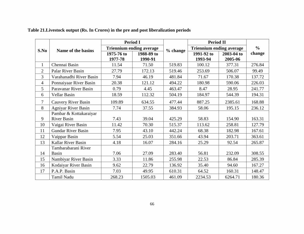
66
Table 21.Livestock output (Rs. In Crores) in the pre and post liberalization periods
S.No Name of the basins
Period I
% change
Period II
%
change Triennium ending average Triennium ending average
1975-76 to
1977-78
1988-89 to
1990-91
1991-92 to
1993-94
2003-04 to
2005-06
1 Chennai Basin 11.54 71.50 519.83 100.12 377.31 276.84
2 Palar River Basin 27.79 172.13 519.46 253.69 506.07 99.49
3 Varahanadhi River Basin 7.94 46.19 481.84 71.67 170.38 137.72
4 Ponnaiyaar River Basin 20.38 121.12 494.22 180.98 590.06 226.03
5 Paravanar River Basin 0.79 4.45 463.47 8.47 28.95 241.77
6 Vellar Basin 18.59 112.32 504.19 184.97 544.39 194.31
7 Cauvery River Basin 109.89 634.55 477.44 887.25 2385.61 168.88
8 Agniyar River Basin 7.74 37.55 384.93 58.06 195.15 236.12
9
Pambar & Kottakaraiyar
River Basin 7.43 39.04 425.29 58.83 154.90 163.31
10 Vaigai River Basin 11.42 70.30 515.37 113.62 258.81 127.79
11 Gundar River Basin 7.95 43.10 442.24 68.38 182.98 167.61
12 Vaippar Basin 5.54 25.03 351.66 43.94 203.71 363.61
13 Kallar River Basin 4.18 16.07 284.16 25.29 92.54 265.87
14
Tambarabarani River
Basin 7.06 27.09 283.40 56.81 232.09 308.55
15 Nambiyar River Basin 3.33 11.86 255.98 22.53 86.84 285.39
16 Kodaiyar River Basin 9.62 22.79 136.92 35.40 94.60 167.27
17 P.A.P. Basin 7.03 49.95 610.31 64.52 160.31 148.47
Tamil Nadu 268.23 1505.03 461.09 2234.53 6264.71 180.36

67
Though net irrigated area has shown positive trend in pre liberalization period and
negative trend in post liberalization period, the net sown area has sown negative trend invariably
in both the periods in all basins. The exceptional case was Vaigai basin, which had shown
positive change in pre liberalization period but negative change in post liberalization period.
Table 22.Net area sown (Area in ha) in the pre and post liberalization periods
S.No Name of the basins
Period I
%
change
Period II
%
change
Triennium ending
average
Triennium ending
average
1975-76
to 1977-
78
1988-89
to 1990-
91
1991-92
to 1993-
94
2003-04
to 2005-
06
1 Chennai Basin 243886 199476 -18.21 219957 162749 -26.01
2 Palar River Basin 526425 422501 -19.74 477556 394085 -17.48
3
Varahanadhi River
Basin 180705 168446 -6.78 188647 161867 -14.20
4 Ponnaiyaar River Basin 690396 662372 -4.06 705021 588745 -16.49
5 Paravanar River Basin 30823 30096 -2.36 33275 29638 -10.93
6 Vellar Basin 388446 380572 -2.03 408936 349809 -14.46
7 Cauvery River Basin 1935939 1951631 0.81 2023300 1782922 -11.88
8 Agniyar River Basin 238855 197875 -17.16 192452 186042 -3.33
9
Pambar & Kottakaraiyar
River Basin 234908 219481 -6.57 233688 207608 -11.16
10 Vaigai River Basin 224491 320862 42.93 318504 274973 -13.67
11 Gundar River Basin 267565 265305 -0.84 259050 217466 -16.05
12 Vaippar Basin 266955 231317 -13.35 215518 166703 -22.65
13 Kallar River Basin 120077 104419 -13.04 87867 71673 -18.43
14
Thambaraparani River
Basin 152746 150469 -1.49 154314 142044 -7.95
15 Nambiar River Basin 68893 65437 -5.02 63701 56931 -10.63
16 Kodaiyar River Basin 77809 77934 0.16 81070 74065 -8.64
17 P.A.P. Basin 164755 147649 -10.38 153854 142684 -7.26
Tamil Nadu 5813675 5595842 -3.75 5816710 5010002 -13.87
It could be clearly noted that the net sown area for past three decades had shown slight
reduction or almost stable. This was mainly due to increase in fallow lands and land put into non-
agricultural purposes. Intensive agriculture followed by policy measures to sustain current area
under agriculture is the need of the hour.
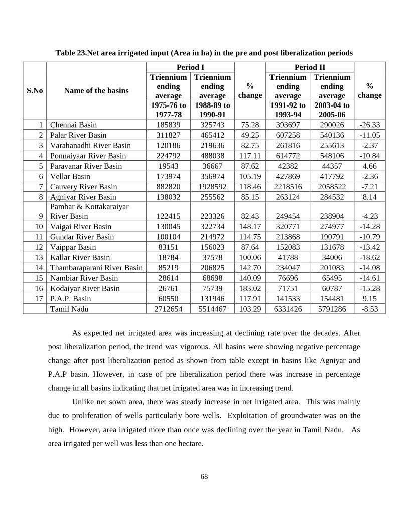
68
Table 23.Net area irrigated input (Area in ha) in the pre and post liberalization periods
S.No Name of the basins
Period I
%
change
Period II
%
change
Triennium
ending
average
Triennium
ending
average
Triennium
ending
average
Triennium
ending
average
1975-76 to
1977-78
1988-89 to
1990-91
1991-92 to
1993-94
2003-04 to
2005-06
1 Chennai Basin 185839 325743 75.28 393697 290026 -26.33
2 Palar River Basin 311827 465412 49.25 607258 540136 -11.05
3 Varahanadhi River Basin 120186 219636 82.75 261816 255613 -2.37
4 Ponnaiyaar River Basin 224792 488038 117.11 614772 548106 -10.84
5 Paravanar River Basin 19543 36667 87.62 42382 44357 4.66
6 Vellar Basin 173974 356974 105.19 427869 417792 -2.36
7 Cauvery River Basin 882820 1928592 118.46 2218516 2058522 -7.21
8 Agniyar River Basin 138032 255562 85.15 263124 284532 8.14
9
Pambar & Kottakaraiyar
River Basin 122415 223326 82.43 249454 238904 -4.23
10 Vaigai River Basin 130045 322734 148.17 320771 274977 -14.28
11 Gundar River Basin 100104 214972 114.75 213868 190791 -10.79
12 Vaippar Basin 83151 156023 87.64 152083 131678 -13.42
13 Kallar River Basin 18784 37578 100.06 41788 34006 -18.62
14 Thambaraparani River Basin 85219 206825 142.70 234047 201083 -14.08
15 Nambiar River Basin 28614 68698 140.09 76696 65495 -14.61
16 Kodaiyar River Basin 26761 75739 183.02 71751 60787 -15.28
17 P.A.P. Basin 60550 131946 117.91 141533 154481 9.15
Tamil Nadu 2712654 5514467 103.29 6331426 5791286 -8.53
As expected net irrigated area was increasing at declining rate over the decades. After
post liberalization period, the trend was vigorous. All basins were showing negative percentage
change after post liberalization period as shown from table except in basins like Agniyar and
P.A.P basin. However, in case of pre liberalization period there was increase in percentage
change in all basins indicating that net irrigated area was in increasing trend.
Unlike net sown area, there was steady increase in net irrigated area. This was mainly
due to proliferation of wells particularly bore wells. Exploitation of groundwater was on the
high. However, area irrigated more than once was declining over the year in Tamil Nadu. As
area irrigated per well was less than one hectare.

69
Table 24.N, P, K input (in lakh tonnes) in the pre and post liberalization periods
S.No Name of the basins
Period I
%
change
Period
II
%
change
Triennium ending
average
Triennium ending
average
1975-76
to 1977-
78
1988-89
to 1990-
91
1991-92
to 1993-
94
2003-04
to 2005-
06
1 Chennai Basin 0.20 0.44 120.40 0.45 0.56 24.72
2 Palar River Basin 0.39 0.73 87.58 0.80 1.05 31.63
3
Varahanadhi River
Basin 0.25 0.51 108.48 0.47 0.45 -4.53
4 Ponnaiyaar River Basin 0.33 0.26 -20.49 0.45 0.80 77.42
5 Paravanar River Basin 0.05 0.10 105.09 0.09 0.08 -17.65
6 Vellar Basin 0.30 0.61 102.24 0.65 1.02 55.80
7 Cauvery River Basin 1.31 2.97 127.29 2.91 3.67 25.99
8 Agniyar River Basin 0.19 0.39 105.87 0.40 0.80 101.96
9
Pambar & Kottakaraiyar
River Basin 0.19 0.21 7.69 0.21 0.65 207.41
10 Vaigai River Basin 0.23 0.50 112.10 0.46 0.68 46.70
11 Gundar River Basin 0.16 0.29 84.80 0.27 0.37 36.24
12 Vaippar Basin 0.13 0.25 98.26 0.20 0.22 7.39
13 Kallar River Basin 0.04 0.07 68.78 0.05 0.06 32.35
14
Thambaraparani River
Basin 0.17 0.33 100.27 0.31 0.10 -66.26
15 Nambiar River Basin 0.06 0.11 99.57 0.10 0.05 -50.16
16 Kodaiyar River Basin 0.06 0.14 154.46 0.13 0.17 25.58
17 P.A.P. Basin 0.10 0.27 161.81 0.24 0.27 13.48
Tamil Nadu 4.15 8.20 97.70 8.21 11.00 34.04
It could be inferred from the table that decline in net sown and net irrigated area resulted
in less usage of NPK. The percentage change was less in post liberalization period compared to
pre liberalization period. Even negative change was noticed in some basins namely Varahanadhi,
Paravanar, Thambaraparani and Nambiar basin during post liberalization period. The basins like
Chennai, Varahanadhi, Ponnaiyaar, Paravanar, Vellar, Cauvery, Agniyar, Vaigai,
Thambaraparani, Nambiar, Kodaiyar, and P.A.P basins have doubled their usage of NPK in pre
liberalization period. NPK consumption in agriculture was increasing at decreasing rate as
evidenced from the above table.

70
Not much fluctuation was noticed in usage except one or two basins like Cauvery basin.
Increase in net irrigated area has led to increased consumption of fertilizers.
Table 25.Labour input (number) in the pre and post liberalization periods
S.No Name of the basins
Period I
%
change
Period II
%
change
Triennium ending
average
Triennium ending
average
1975-76
to 1977-
78
1988-89
to 1990-
91
1991-92
to 1993-
94
2003-04
to 2005-
06
1 Chennai Basin 267652 378884 41.56 389087 388521 -0.15
2 Palar River Basin 520572 729151 40.07 758329 821497 8.33
3
Varahanadhi River
Basin 190216 276183 45.19 295534 364578 23.36
4 Ponnaiyaar River Basin 488505 749170 53.36 813726 1057408 29.95
5 Paravanar River Basin 31865 46871 47.09 50922 67041 31.66
6 Vellar Basin 349523 505665 44.67 554886 766676 38.17
7 Cauvery River Basin 1581150 2122578 34.24 2328366 3317327 42.47
8 Agniyar River Basin 136972 204479 49.29 232979 369695 58.68
9
Pambar & Kottakaraiyar
River Basin 122716 198438 61.71 215515 271685 26.06
10 Vaigai River Basin 358001 514992 43.85 535612 537236 0.30
11 Gundar River Basin 208467 295261 41.63 304487 296177 -2.73
12 Vaippar Basin 212024 274146 29.30 271745 220760 -18.76
13 Kallar River Basin 59611 79114 32.72 78874 66311 -15.93
14
Thambaraparani River
Basin 222006 285500 28.60 291607 293568 0.67
15 Nambiar River Basin 80448 103610 28.79 104290 95596 -8.34
16 Kodaiyar River Basin 130573 163457 25.18 148770 42115 -71.69
17 P.A.P. Basin 171063 205728 20.26 203480 180528 -11.28
Tamil Nadu 5131365 7133227 39.01 7578207 9156718 20.83
The statements like rural population is moving out of agriculture and agriculture suffers
from non-availability of laborers have been proved by the data given in the above table. After
liberalization, percentage change in labour use in agriculture was negative in few basins and was
less in other basins compared to pre liberalization period. In pre liberalization period there was
positive percentage change in all river basins. From the tables it can be seen that labour usage
showed a declining trend after 1990s due to introduction of mechanization.

71
Table 26.Cattle input (number) in the pre and post liberalization periods
S.No Name of the basins
Period I
%
change
Period II
%
change
Triennium ending
average
Triennium ending
average
1975-76
to 1977-
78
1988-89
to 1990-
91
1991-92
to 1993-
94
2003-04
to 2005-
06
1 Chennai Basin 744437 644478 -13.43 670935 573156 -14.57
2 Palar River Basin 1607469 1356681 -15.60 1382576 1107548 -19.89
3
Varahanadhi River
Basin 497988 424643 -14.73 434911 355763 -18.20
4
Ponnaiyaar River
Basin 1768466 1608348 -9.05 1507023 1396512 -7.33
5 Paravanar River Basin 74539 63009 -15.47 63883 54448 -14.77
6 Vellar Basin 1097054 1018839 -7.13 1006174 928847 -7.69
7 Cauvery River Basin 4724953 4696622 -0.60 4285740 3711614 -13.40
8 Agniyar River Basin 581628 577639 -0.69 625020 479306 -23.31
9
Pambar &
Kottakaraiyar 373945 410804 9.86 469229 382388 -18.51
10 Vaigai River Basin 523930 545132 4.05 514994 393209 -23.65
11 Gundar River Basin 321104 340546 6.05 344715 273709 -20.60
12 Vaippar Basin 248051 254536 2.61 244721 299830 22.52
13 Kallar River Basin 157484 147478 -6.35 112556 77643 -31.02
14
Thambaraparani River
Basin 259428 243512 -6.14 186833 397172 112.58
15 Nambiar River Basin 109035 101332 -7.06 79127 129975 64.26
16 Kodaiyar River Basin 138948 115838 -16.63 111702 100352 -10.16
17 P.A.P. Basin 297462 299064 0.54 251205 202322 -19.46
Tamil Nadu 13525920 12848500 -5.01 12291346 10863794 -11.61
Liberalisation policies on agriculture did not show any positive impact on livestock
population. All basins except Nambiar basin had shown negative percentage change in post
liberalization period. Even in pre liberalization period, also most of the basins showed negative
percentage change except Pambar & Kottakaraiyar, Vaigai, and Gundar and Vaippar river
basins.

72
In river basins like Pambar & Kottaikaraiyar, Vaippar, Tambarabarani and Nambiar
showed increase in cattle input usage from the base year (1975-76 to 2005-06 and all other river
basins had shown decline in cattel input usage for the above said period. Comparing cattle input
in base year and current year period, Tamil Nadu as a whole showed negative change.
The table also shows decrease in cattle inputs in all basins except Thambaraparani.
Comparing base year (1975-76) cattle input used in agriculture and present data (2005-06)
number itself reduced. There is wide scope for bringing livestock rearing and dairying as a
commercial venture in Tamil Nadu.
Table 27.Poultry input (number) in the pre and post liberalization periods
S.No Name of the basins
Period I
%
change
Period II
%
change
Triennium ending
average
Triennium ending
average
1975-76
to 1977-
78
1988-89
to 1990-
91
1991-92
to 1993-
94
2003-04
to 2005-
06
1 Chennai Basin 984989 863424 -12.34 936027 988312 5.59
2 Palar River Basin 1066035 1093367 2.56 1217672 1358716 11.58
3
Varahanadhi River
Basin 387383 343528 -11.32 361679 298840 -17.37
4 Ponnaiyar River Basin 1262555 1399800 10.87 1385879 3301544 138.23
5 Paravanar River Basin 58261 51665 -11.32 53361 48532 -9.05
6 Vellar Basin 1300313 1996879 53.57 2242363 6751094 201.07
7 Cauvery River Basin 5368687 7939348 47.88 8858910 47897893 440.67
8 Agniyar River Basin 735319 769482 4.65 798651 684494 -14.29
9
Pambar &
Kottakaraiyar 553990 604161 9.06 694833 943135 35.74
10 Vaigai River Basin 696536 761271 9.29 781816 1445188 84.85
11 Gundar River Basin 410809 470487 14.53 550945 781329 41.82
12 Vaippar Basin 294755 375588 27.42 504592 852462 68.94
13 Kallar River Basin 208734 220442 5.61 243992 193003 -20.90
14
Tambarabarani River
Basin 495098 520492 5.13 572784 947815 65.48
15 Nambiyar River Basin 205708 210806 2.48 228070 325309 42.64
16 Kodaiyar River Basin 483809 422250 -12.72 400744 450061 12.31
17 P.A.P. Basin 305400 482835 58.10 592908 15077533 2442.98
Tamil Nadu 14818381 18525822 25.02 20425226 82345259 303.15
73
Varahanadhi, Paravanar, Agniyar, and Kallar basins had showed negative percentage
change in post liberalization period where the poultry population itself was in decline trend
comparing base year and current year data.
All other river basins showed positive percentage change in poultry population. Basins
like Cauvery and P.A.P basins had tremendous growth of poultry. Most of the poultry farms
were commercial units in these basins.
Poultry has become commercial venture during current decade and it could be referred
from the figures 15 and 16 where except one or two basins all other basins showed increasing
trend in poultry population after 2000. Development of poultry industry in agricultural farms led
to more area under maize and other cereals and development of feed units.

74
CHAPTER XII
Comparison of crop out per unit of sown area and per unit of water potential
12. Comparison of crop out per unit of sown area and per unit of water potential
It is observed that the value of crop output per ha of area has varied among the basins.
The increase in crop output was maximum in Paravanar basin followed by Vellar and
Varahanadhi basin. Lowest crop output was noticed in Kallar, Vaippar and Nambiar basins. The
reason for the vast difference was mainly due to the types of crops grown and the extend of crop
area. In the case of value of crop output per MCM, the value was higher in the case of
Ponnaiyaar basin followed by Vellar and Cauvery basins. Lower crop output was observed in
Thambaraparani basin followed by Vaippar and Nambiar basins. There is some correlation
among the crop outputs between the crop area and water storage. The reason for the higher
output from the basins is that the water potential is comparatively lower in these basins and the
crop is mainly diversified towards high value crops (Table 28).
Table 28. Value of Crop Output per ha of Sown Area
Basin 1975-76 80-81 85-86 90-91 95-96 2000-01 2005-2006
Chennai 4853 8184 15003 25884 73782 93215 93114
Palar River 7533 13057 18427 26878 81279 100068 126827
Varahanadhi River 7627 13602 27075 40014 108774 188492 231602
Ponnaiyaar River 5468 10351 18738 25135 64906 83280 190158
Paravanar River 8455 15078 30839 46574 123385 222839 274798
Vellar 7728 13559 23782 31509 83351 114906 235237
Cauvery River 10071 13447 17504 22229 58071 82383 131161
Agniyar River 3171 4598 9812 15685 40418 54732 125860
Pambar & Kottakaraiyar River 4483 5290 8996 15527 24018 43298 56927
Vaigai River 14718 8505 14516 23559 48513 70338 74606
Gundar River 5973 5444 9716 19560 26880 48019 49027
Vaippar 3961 4427 8453 28430 26083 44459 46595
Kallar River 4639 4363 8470 13009 5199 14499 15985
Thambaraparani River 7762 7300 14172 27510 41374 55503 50885
Nambiar River 6582 6182 12711 22555 29516 42615 47355
Kodaiyar River 5357 4650 18430 12849 9968 17201 101637
P.A.P. 18992 19262 27528 23483 64519 68474 111508

75
Figure 6. Crop output/ha of net sown area
Crop output / ha of net sown area
5,000
30,000
55,000
80,000
105,000
130,000
155,000
180,000
205,000
230,000
255,000
280,000
1975-76 80-81 85-86 90-91 95-96 2000-01 2005-2006
Rs
/ h
a
Chennai Palar River Varahanadhi RiverPonnaiyar River Paravanar River VellarCauvery River Agniyar River Pambar & Kottakaraiyar RiverVaigai River Gundar River VaipparKallar River Tambarabarani River Nambiyar RiverKodaiyar River P.A.P.
c

76
Table 29. Value of crop output per MCM of water potential
S.No Basin 1975-76 80-81 85-86 90-91 95-96 2000-01 2005-2006
1 Chennai 579119 798875 1651047 2715940 7703252 8714829 8364944
2 Palar River 898152 1247314 2057214 2640763 8630699 9497440 12304077
3 Varahanadhi River 705428 1137381 2624008 3552727 10323286 17312708 20283824
4 Ponnaiyaar River 1304490 2004029 4495255 5787412 15359238 19161418 40249549
5 Paravanar River 678510 1139579 2726138 3681854 10668863 19139062 22420026
6 Vellar 1217789 1897940 3751369 4872577 13709440 18638038 36177428
7 Cauvery River 2199458 2760756 3779911 4871066 12487879 17787266 27799468
8 Agniyar River 371719 435306 1128755 1468825 2903593 5407976 12446166
9 Pambar & Kottakaraiyar River 634079 694266 1258176 2172724 2785534 5486064 7392297
10 Vaigai River 1272589 1093899 1659186 2948961 5151004 7682754 8388698
11 Gundar River 1169910 1173428 1835690 3915834 4385686 7805190 8166278
12 Vaippar 563275 635856 1070477 3552093 2484029 4000726 4458871
13 Kallar River 2297539 2478872 4493891 5961352 1844608 4589545 5452148
14 Thambaraparani River 488102 526625 954707 2062737 2598607 3446250 3617932
15 Nambiar River 837667 887970 1717572 3127851 3426203 4746596 5878630
16 Kodaiyar River 339575 274830 1122387 786576 640593 1029929 5973029
17 P.A.P. 2661556 2588438 3773529 2863020 7749420 8447839 13616397

77
Crop output / per unit of water
0
5,000,000
10,000,000
15,000,000
20,000,000
25,000,000
30,000,000
35,000,000
40,000,000
45,000,000
1975-76 80-81 85-86 90-91 95-96 2000-01 2005-2006
MC
M
/ h
a
Chennai Palar River Varahanadhi RiverPonnaiyar River Paravanar River VellarCauvery River Agniyar River Pambar & Kottakaraiyar RiverVaigai River Gundar River VaipparKallar River Tambarabarani River Nambiyar RiverKodaiyar River P.A.P.
Figure 7. Crop output/per unit of water
78
CHAPTER XIII
Results of TFP analysis
13. Results of TFP analysis
Using DEA methodology described already, total factor productivity was computed for
all river basins for three decades starting from 1975-76 to and 2005-06. Technical efficiency
change was decomposed into pure efficiency change and scale efficiency change. The details of
technical efficiency change, technical change and TFP change for each basin and for each year
are provided in Appendix-II. The geometric mean values are summarized in Table.30 the graphs
of trends in TFP for small, medium, and large basins are presented in Figs.
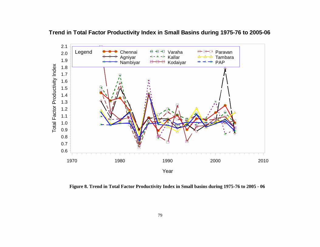
79
Tota
l F
acto
r P
rod
uctivi
ty I
nd
ex
0.6
0.7
0.8
0.9
1.0
1.1
1.2
1.3
1.4
1.5
1.6
1.7
1.8
1.9
2.0
2.1
Year
1970 1980 1990 2000 2010
Trend in Total Factor Productivity Index in Small Basins during 1975-76 to 2005-06
Legend Chennai Varaha ParavanAgniyar Kallar TambaraNambiyar Kodaiyar PAP
Figure 8. Trend in Total Factor Productivity Index in Small basins during 1975-76 to 2005 - 06
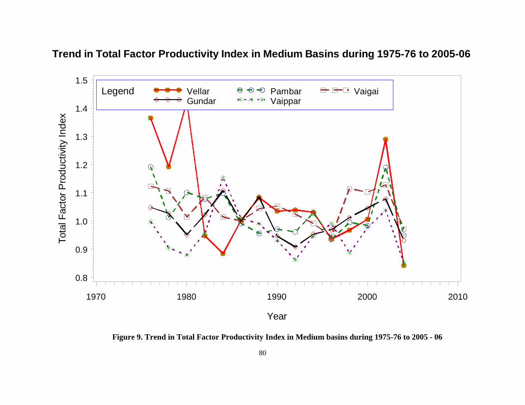
80
Tota
l F
acto
r P
rod
uctivi
ty I
nd
ex
0.8
0.9
1.0
1.1
1.2
1.3
1.4
1.5
Year
1970 1980 1990 2000 2010
Trend in Total Factor Productivity Index in Medium Basins during 1975-76 to 2005-06
Legend Vellar Pambar VaigaiGundar Vaippar
Figure 9. Trend in Total Factor Productivity Index in Medium basins during 1975-76 to 2005 - 06

81
Tota
l F
acto
r P
rod
uctivi
ty I
nd
ex
0.7
0.8
0.9
1.0
1.1
1.2
1.3
1.4
1.5
1.6
Year
1970 1980 1990 2000 2010
Trend in Total Factor Productivity Index in Large Basins during 1975-76 to 2005-06
Legend palar Ponnaiya Cauvery
Figure10. Trend in Total Factor Productivity Index in Large basins during 1975-76 to 2005 - 06

82
Table 30. Mean Technical Efficiency Change, Technical Change and TFP
Change, during three decades in the seventeen river basins of Tamil Nadu
Basin Efficiency
change
Technical
change
Scale efficiency
change
Total factor
productivity change
Chennai
1975-76 to 1990-91 0.9976 1.0877 0.9976 1.0849
1991-92 to 2005-06 1.0103 1.0024 1.0103 1.0126
1975-76 to 2005-06 1.0039 1.0442 1.0039 1.0481
Palar
1975-76 to 1990-91 0.9998 1.1434 0.9998 1.1431
1991-92 to 2005-06 0.9961 1.0102 0.9961 1.0063
1975-76 to 2005-06 0.9980 1.0747 0.9980 1.0725
Varahanadhi
1975-76 to 1990-91 0.9995 1.1104 0.9995 1.1098
1991-92 to 2005-06 1.0015 1.0063 1.0015 1.0080
1975-76 to 2005-06 1.0005 1.0571 1.0005 1.0577
Ponnaiyar
1975-76 to 1990-91 1.0229 1.1431 1.0229 1.1693
1991-92 to 2005-06 0.9437 1.0060 0.9437 0.9494
1975-76 to 2005-06 0.9825 1.0723 0.9825 1.0536
Paravanar
1975-76 to 1990-91 1.0000 1.0481 1.0000 1.0481
1991-92 to 2005-06 1.0000 0.9864 1.0000 0.9864
1975-76 to 2005-06 1.0000 1.0168 1.0000 1.0168
Vellar
1975-76 to 1990-91 0.9909 1.1348 0.9909 1.1245
1991-92 to 2005-06 0.9757 1.0212 0.9757 0.9965
1975-76 to 2005-06 0.9832 1.0765 0.9832 1.0586
Cauvery
1975-76 to 1990-91 0.9895 1.1199 0.9895 1.1080
1991-92 to 2005-06 0.9856 1.0073 0.9856 0.9929
1975-76 to 2005-06 0.9876 1.0621 0.9876 1.0489
Agniyar
1975-76 to 1990-91 1.0037 1.0587 1.0037 1.0628
1991-92 to 2005-06 0.9637 1.0140 0.9637 0.9770
1975-76 to 2005-06 0.9835 1.0361 0.9835 1.0190
Pambar-Kotta
1975-76 to 1990-91 0.9974 1.0758 0.9974 1.0731
1991-92 to 2005-06 1.0065 0.9898 1.0065 0.9963
1975-76 to 2005-06 1.0019 1.0319 1.0019 1.0340
Vaigai
1975-76 to 1990-91 0.9870 1.0720 0.9870 1.0582
1991-92 to 2005-06 1.0236 1.0048 1.0236 1.0284

83
1975-76 to 2005-06 1.0051 1.0379 1.0051 1.0432
Gundar
1975-76 to 1990-91 0.9876 1.0717 0.9876 1.0581
1991-92 to 2005-06 1.0260 0.9723 1.0260 0.9978
1975-76 to 2005-06 1.0066 1.0208 1.0066 1.0275
Vaippar
1975-76 to 1990-91 0.9872 1.0272 0.9872 1.0140
1991-92 to 2005-06 1.0045 0.9436 1.0045 0.9480
1975-76 to 2005-06 0.9958 0.9845 0.9958 0.9804
Kallar
1975-76 to 1990-91 1.0000 1.0296 1.0000 1.0296
1991-92 to 2005-06 1.0000 1.0021 1.0000 1.0021
1975-76 to 2005-06 1.0000 1.0158 1.0000 1.0158
Tambaraparani
1975-76 to 1990-91 0.9981 1.0086 0.9981 1.0067
1991-92 to 2005-06 0.9942 0.9833 0.9942 0.9775
1975-76 to 2005-06 0.9961 0.9959 0.9961 0.9920
Nambiyar
1975-76 to 1990-91 1.0000 0.9907 1.0000 0.9907
1991-92 to 2005-06 1.0000 0.9912 1.0000 0.9912
1975-76 to 2005-06 1.0000 0.9910 1.0000 0.9910
Kodaiyar
1975-76 to 1990-91 1.0004 0.9742 1.0004 0.9746
1991-92 to 2005-06 1.0000 1.0056 1.0000 1.0056
1975-76 to 2005-06 1.0002 0.9898 1.0002 0.9899
PAP
1975-76 to 1990-91 0.9998 0.9691 0.9998 0.9690
1991-92 to 2005-06 1.0033 0.9773 1.0033 0.9804
1975-76 to 2005-06 1.0015 0.9732 1.0015 0.9747
13.1. Overall TFP growth
From the above table it could be seen that the mean TFP between basins ranged between
0.9747 to 1.0725. Palar basin had the highest TFP of 1.0725 and PAP had the least TFP of 0.9747.
Except Vaippar, Thambaraparani, Nambiar and PAP, in all other 13 basins the TFP for the
three decades is greater than 1 indicating positive TFP growth in all these basins. In the 4 basins
though the TFP is less than 1, it ranges from 0.9747 to 0.992 which are very close to 1. Thus, we
can conclude in general that there was total factor productivity growth in Tamil Nadu over the past
three decades.

84
Further, in all basins except Vaippar, Tambarani, Nambiar, Kodaiyar and PAP, the
technical change was more than one indicating technological advancements in agriculture in these
basins. Nevertheless, the overall efficiency change was very close to 1 in all the basins. This
means that the total factor growth is contributed mainly by technology and there is not much
change in efficiency. Similarly, there is not much change in overall scale efficiencies.
Further, during the pre-liberalization period, 14 river basins have registered positive TFP
growth. Three basins, viz., Nambiar, Kodaiyar, and PAP have shown TFPs which are close to 1.
During the post-liberalization period, 11 basins have TFPs less than but very close to 1 and 6
basins have TFPs greater than 1 (Table31 ). A simple t-test was carried out to test the significance
of the difference between the TFPs of the two periods. The test rejected the null hypothesis (p-
value=0.00041) that the mean TFPs are equal in the two periods. The averages of the TFPs in the
pre and post liberalization periods are 1.0603 and 0.9975. These results imply that over all
liberalization was not beneficial to agricultural growth in the river basins of Tamil Nadu.
Table 31.Table Mean TFPs in three periods
Basin
Period1(1975-76
to 1990-91)
Period2(Period1(1991-
92 to 2005-06)
Overall (1975-76
to 2005-06)
Chennai 1.0849 1.0126 1.0481
Palar 1.1431 1.0063 1.0725
Varaha 1.1098 1.1098 1.0577
Ponnaiyaar 1.1693 0.9494 1.0536
Paravanar 1.0481 0.9864 1.0168
Vellar 1.1245 0.9965 1.0586
Cauvery 1.1080 0.9929 1.0489
Agniyar 1.0628 0.9770 1.0190
Pambar 1.0731 0.9963 1.0340
Vaigai 1.0582 1.0284 1.0432
Gundar 1.0581 0.9978 1.0275
Vaippar 1.0140 0.9480 0.9804
Kallar 1.0296 1.0021 1.0158
Tambara 1.0067 0.9775 0.9920
Nambiyar 0.9907 0.9912 0.9910
Kodaiyar 0.9746 1.0056 0.9899
PAP 0.9690 0.9804 0.9747

85
13.2. Individual basin TFP
The TFP growth rates of individual basins have been presented in Appendix. Detailed
discussions are presented below.
The average total factor productivity change for Chennai basin was more than one
indicating that agricultural production is technically efficient. Both pre liberalization period TFP
and post liberalization period TFP were more than one.
In Palar basin the range of efficiency change was from 0.772 to 1.506. There was not much
difference in TFP and other efficiency change between the two periods. It was more than one
indicating that Palar basin was technically efficient in using inputs.
In Varahanadhi basin TFP was more than one in pre and post liberalization period
indicating that the basin was technically sound. TFP range was from 0.705 to 1.515.
Though in Ponnaiyaar river basin average TFP was more than one, in post liberalization
period it was less than one i.e. 0.949. In pre liberalization period, it was 1.169. Similarly,
efficiency change was less than one in post liberalization period whereas technical efficiency
change was more than one in both the period and it was 1.184 in pre liberalization period and
1.016 in post liberalization period.
In Paravanar basin, the average TFP was 1.034 and there was slight difference in TFP in
pre (0.989) and post liberalization period (1.079). The efficiency change was one in both periods
and the change in TFP was due to technical efficiency change.
In vellar basin the average TFP was more than one (1.070) in the last three decades. There
was no difference noted in pre and post liberalization periods. Nevertheless, the efficiency change
was less than one and the technical change was more than one.
The average TFP was nearing one in post libralisation period and it was above one in pre
liberalization period (1.115). Though technical change was more than one in both periods, the
efficiency change was less than one or nearing one indicating there is wide scope to improve the
efficiency of inputs used for agricultural production.
There is a possibility for improving efficiency of inputs in Agniyar basin as there was
slight reduction in efficiency change from 1.013 (pre liberalization period) to 0.986 (post
liberalization period). Further improvement in TFP should come only from technology
development.

86
Though average TFP was more than one in both periods in Pambar & Kottakaraiyar river
basin, there was slight reduction in TFP and technical change in post liberalization period
indicating that technology improvement is the need of the hour. Further improvement in TFP will
come only from technology change and not from efficiency of inputs.
The same trend was noted in Vaigai basin as in case of Pambar & Kottakaraiyar basin.
Though efficiency of inputs have improved after liberalization period there was not much of
improvement in technology. It was evidenced from the table that technical change was reduced
from 1.078 in pre liberalization period to 1.008 in post liberalization period. Therefore, TFP also
showed slight reduction in post period.
Gundar river basin also followed the same trend as that of Pambar and Vaigai basin. Period
II i.e. post liberalization period faced reduced TFP and technical change coefficients. There was
slight improvement in efficiency change coefficients.
The total factor productivity was less than one in period II (0.952) compared to pre
liberalization period (1.028) in Vaippar basin. The average TFP for the last three decades was
0.99. The average technical change was nearing one but it was less than period I. Without
improving technology liberalization policies alone would not bring prosperity in agriculture and
livestock.
In Kallar basin it was inferred from the table that changes in total factor productivity was
mainly due to technical change. As efficiency change was one and there was no change in
efficiency of inputs in last three decades, any development activity should focus on technical
improvement. This was further stressed by the fact that reducing trend in total factor productivity
after liberalization period.
There was reduction in TFP in Thambaraparani basin as shown in the table. TFP has
reduced from 1.019 in pre liberalization period to 0.984 in post liberalization period. Technical
change also showed the same trend and it was less than one in post liberalization period. There
was no change in efficiency coefficient in these two period and it was nearing one i.e. 0.998.
In Nambiar basin changes in total factor productivity was fully contributed by technical
changes and not due to the efficiency of inputs in agriculture and allied sector. There was no
change in TFP in two periods indicating that there was not much change in technology adopted by
the farmers. Efficiency of inputs also needs attention, as it remained same in both the periods.
In Kodaiyar basin also changes in total factor productivity was fully contributed by
technical changes and not due to the efficiency of inputs in agriculture and allied sector.
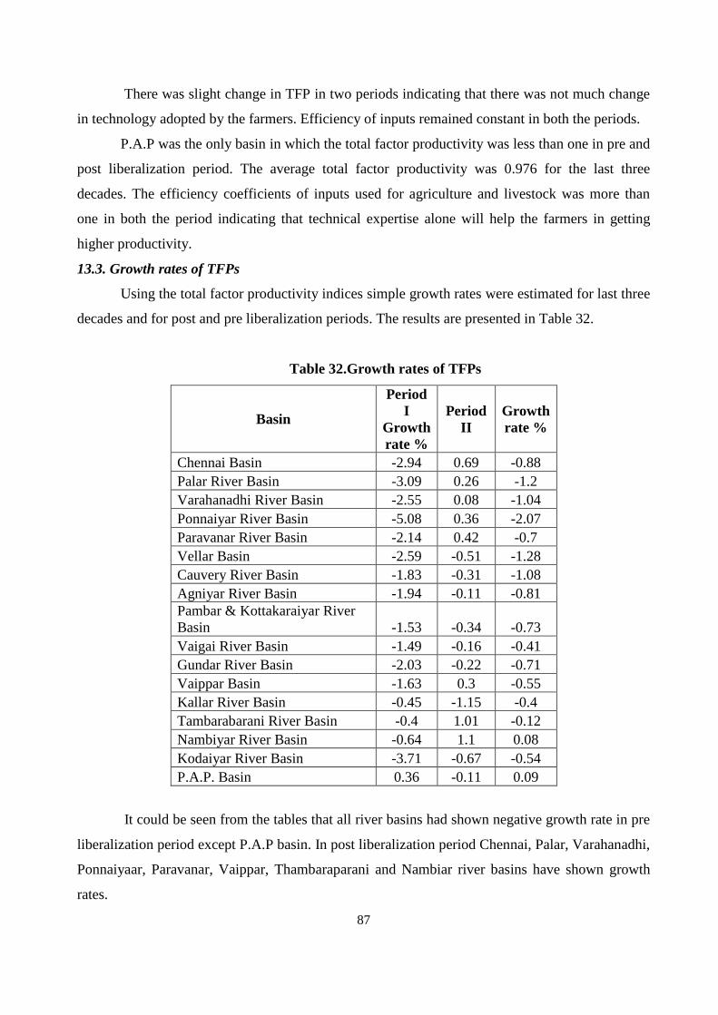
87
There was slight change in TFP in two periods indicating that there was not much change
in technology adopted by the farmers. Efficiency of inputs remained constant in both the periods.
P.A.P was the only basin in which the total factor productivity was less than one in pre and
post liberalization period. The average total factor productivity was 0.976 for the last three
decades. The efficiency coefficients of inputs used for agriculture and livestock was more than
one in both the period indicating that technical expertise alone will help the farmers in getting
higher productivity.
13.3. Growth rates of TFPs
Using the total factor productivity indices simple growth rates were estimated for last three
decades and for post and pre liberalization periods. The results are presented in Table 32.
Table 32.Growth rates of TFPs
Basin
Period
I
Growth
rate %
Period
II
Growth
rate %
Chennai Basin -2.94 0.69 -0.88
Palar River Basin -3.09 0.26 -1.2
Varahanadhi River Basin -2.55 0.08 -1.04
Ponnaiyar River Basin -5.08 0.36 -2.07
Paravanar River Basin -2.14 0.42 -0.7
Vellar Basin -2.59 -0.51 -1.28
Cauvery River Basin -1.83 -0.31 -1.08
Agniyar River Basin -1.94 -0.11 -0.81
Pambar & Kottakaraiyar River
Basin -1.53 -0.34 -0.73
Vaigai River Basin -1.49 -0.16 -0.41
Gundar River Basin -2.03 -0.22 -0.71
Vaippar Basin -1.63 0.3 -0.55
Kallar River Basin -0.45 -1.15 -0.4
Tambarabarani River Basin -0.4 1.01 -0.12
Nambiyar River Basin -0.64 1.1 0.08
Kodaiyar River Basin -3.71 -0.67 -0.54
P.A.P. Basin 0.36 -0.11 0.09
It could be seen from the tables that all river basins had shown negative growth rate in pre
liberalization period except P.A.P basin. In post liberalization period Chennai, Palar, Varahanadhi,
Ponnaiyaar, Paravanar, Vaippar, Thambaraparani and Nambiar river basins have shown growth
rates.

88
All other river basins showed negative growth rate in post liberalization period. The
growth rate was mainly due to efficiency of inputs used for agriculture and livestock.
Efficiency change has contributed much to the total factor productivity. But overall
growth rate ie growth rate of total factor productivity for last three decades was negative for all
river basins except Nambiar and P.A.P river basins.
From above results, it could be concluded that though most of the river basins have shown
total factor productivity more than one, there was no growth in the total factor productivity in last
three decades except in one or two basins.

89
CHAPTER XIV
Cumulative TFP indices
14. Cumulative TFP indices
Another approach to analyze the change of productivity is using cumulative TFP index.
The values of these indices for all basins are provided in the Appendix-IV. In the figure, we
display the cumulative TFP index of small, medium, and large basins. In the small basins, this
index fluctuates drastically from 0.296 to 1.475. The highest value corresponding to Kallar basin
for three year 1986-87 and the lowest value belongs to Kodaiyar for the year 1987-88. In fact, the
cumulative TFP for all years are less than 1. This means that compared with the year 1975-76 in
all the years, the TFP for this basin is very much lower. The same type of result can be drawn with
respect to other small basins also except in few cases for some years. In medium basins, the TFP
indices varied from 0.605 to 1.598 and the corresponding values for large basins are respectively
0.543 and 1.907.
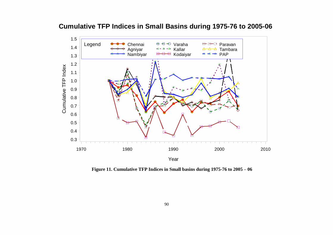
90
Cu
mu
lative
TF
P I
nd
ex
0.3
0.4
0.5
0.6
0.7
0.8
0.9
1.0
1.1
1.2
1.3
1.4
1.5
Year
1970 1980 1990 2000 2010
Cumulative TFP Indices in Small Basins during 1975-76 to 2005-06
Legend Chennai Varaha ParavanAgniyar Kallar TambaraNambiyar Kodaiyar PAP
Figure 11. Cumulative TFP Indices in Small basins during 1975-76 to 2005 – 06
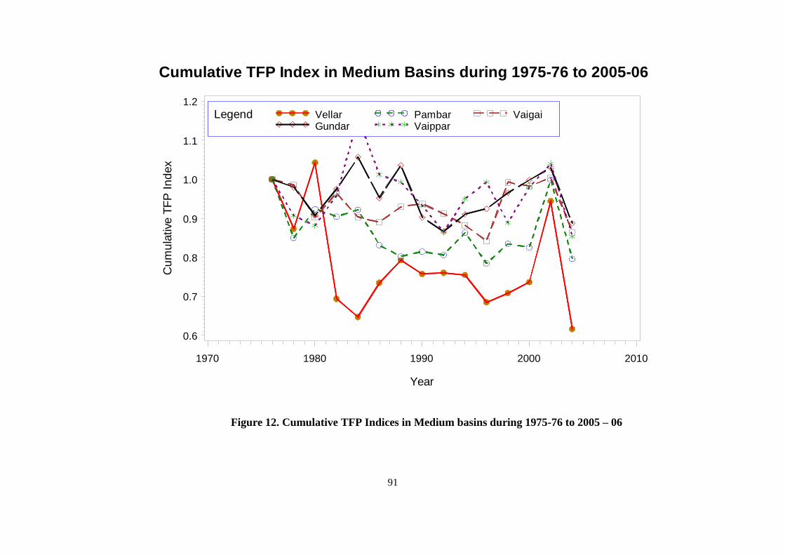
91
Cu
mu
lative
TF
P I
nd
ex
0.6
0.7
0.8
0.9
1.0
1.1
1.2
Year
1970 1980 1990 2000 2010
Cumulative TFP Index in Medium Basins during 1975-76 to 2005-06
Legend Vellar Pambar VaigaiGundar Vaippar
Figure 12. Cumulative TFP Indices in Medium basins during 1975-76 to 2005 – 06

92
Cu
mu
lative
TF
P I
nd
ex
0.7
0.8
0.9
1.0
1.1
1.2
1.3
1.4
1.5
1.6
Year
1970 1980 1990 2000 2010
Cumulative TFP Indices in Large Basins during 1975-76 to 2005-06
Legend palar Ponnaiya Cauvery
Figure 13. Cumulative TFP Indices in Large basins during 1975-76 to 2005 - 06

93
CHAPTER XV
Results of DEA analysis
15. Results of DEA analysis
The TFP growth analysis provides trend in agricultural growth for the past three decades.
However, it does not provide options for further improvement in production and inputs usage.
With this in view DEA was performed. Given that we have 31 annual observations for 17 river
basins, we can perform DEA for each year by solving 17 Linear Programs for each year resulting
in a total of 527 LP problems. This will add to complexity in presenting the results. Further to
formulate policy options for future years, it will be more appropriate to perform DEA for the latest
period, i.e., 2005-06. Hence, DEA was performed for the period 2005-06 and the results are
discussed with a orientation for recommending policies for efficient utilization of resources.
The models with CRS technology assume that an increase in inputs will result in a
proportional increase in outputs. However, it is difficult to find such a linear relationship between
inputs and production in agriculture. For example, in agriculture, when the water volume applied
to crops is increased, we do not necessarily obtain a linearly proportional increase in agricultural
production. In order to account for this effect, the DEA model for variable-returns-to-scale (BCC)
was developed [Banker et.al, 1984] and the same model has been used in the present study.
The other essential characteristic of DEA models is orientation. The output-oriented model
refers to the capacity of a DMU to achieve the maximum volume of production (output) with the
available inputs, while the ability to maintain the same capacity of production using a minimum of
inputs is known as the input-oriented model. Input-oriented efficiency scores range between 0 and
1.0, and whereas output-oriented efficiency scores range between 1.0 to infinity; in both cases, 1.0
is efficient. In agriculture, it is very important not only to produce maximum production but also
to use inputs efficiently. Hence, both orientations (with VRS technology) are used in the present
study and the results are discussed below.
15.1. DEA with VRS technology and Output Orientation.
Table.33 provides a summary of Output Oriented VRS DEA, CRS DEA efficiency scores
and scale efficiencies for each river basin. The table shows that out of 17 basins, 13 basins are
100% VRS efficient and out of these efficient basins 9 basins are scale efficient also. Palar,

94
Cauvery, Vaippar and PAP basins are though VRS efficient, they are scale inefficient as their CRS
efficiencies are less than 1. Agniyar, Pambar & Kottakaraiyar, Vaigai and Gundar are inefficient
as their efficiency scores are less than 1.
It is interesting to note that these basins are CRS inefficient also. Their efficiency scores
range between 0.642 (Pambar & Kottakaraiyar) and 0.994(Vaigai). The average score of all the
basins is 0.969 and all these basins are located adjacently.
Table 33. Output Oriented VRS DEA model scores for the River basins of Tamil Nadu
Basin
No. Basin Name
Efficiency-
VRS
Efficiency-
CRS
Efficiency-
Scale
1 Chennai 1 1 1
2 Palar 1 0.798 0.798
3 Varahanadhi 1 1 1
4 Ponnaiyar 1 1 1
5 Paravanar 1 1 1
6 Vellar 1 1 1
7 Cauvery 1 0.898 0.898
8 Agniyar 0.864 0.798 0.924
9 Pambar & Kottakaraiyar 0.642 0.493 0.768 10 Vaigai 0.994 0.692 0.696
11 Gundar 0.967 0.658 0.680
12 Vaippar 1 0.839 0.839
13 Kallar 1 1 1
14 Tambarabarani 1 1 1
15 Nambiyar 1 1 1
16 Kodaiyar 1 1 1
17 P.A.P. 1 0.897 0.897
Mean 0.969 0.887 0.912
Data envelopment analysis identifies for each inefficient unit a set of excellent units, called
a peer group that can be utilized as benchmarks (reference basins) for improvement, and also
allows computing the projected values of inputs and outputs to make them efficient. The projected
values are computed as a linear combination of the values of the benchmarks using suitable
weights derived from DEA. Table.34 provides a summary of the benchmark basins for each
inefficient basin and the projected values of inputs and outputs for all the basins.
Pambar & Kottakaraiyar basin is the least inefficient basin with an efficiency score of
0.642. For this basin, water, land, labour and resources do not fully contribute to the agricultural
production, and the usage patterns should be improved for all inputs according to the
95
corresponding efficient basins, viz., Vellar (0.046), Ponnaiyaar (0.034), Chennai (0.407), and
Kodaiyar (0.512).
In other words Pambar & Kottakaraiyar basin can follow the cropping pattern and input
use as done in its benchmark basins and there is scope for further improvement in crop and
livestock output.
A simple calculation with actual and projected outputs shows that this basin can reduce the
labor by 10%, net irrigated area by 18%, NPK usage by 55%, net sown area by 29% but still
achieve and increase in each of the two outputs by 56%. Thus, for this basin there is scope for
increase in production with reduction in inputs. In order to achieve this it can follow the
combination of cropping patterns and inputs usage of Kodaiyar and Chennai basins, which are its
two major benchmark basins.
Agniyar is the next inefficient basin with a efficiency score of 0.864. Its benchmark basins
are Ponnaiyar(0.013), Kodaiyar (0.021), Chennai (0.464) and Varahanadhi (0.501). The projected
outputs for this basin are Rs.2887.3 (crores) for crop and Rs. 258.2(crores) for livestock.
Calculations with actual outputs show that this basin can increase each one of these two outputs by
16% and at the same time reduce net-irrigated area by 6%, NPK usage by 37%, Net area sown by
10% and cattle by 4%. This improvement can be reached if this basin follows the cropping and
input usage patterns of its major benchmark basins viz., Varahanadhi and Chennai.
Gundar is the third inefficient basin and its output oriented VRS efficiency score is 0.967.
Its benchmark basins are Kodaiyar (0.572), Chennai (0.314), Cauvery (0.006), and Kallar (0.108).
There is potential for increasing its two outputs by 3% with a reduction in labour by 43%, net
irrigated area by 23%, NPK usage by 21% and net sown area by 46%. Since Kodaiyar and
Chennai are its benchmark basins with maximum weights, Gundar basin can achieve the above
said targets by following the cropping pattern and input usage of these two basins.
Vaigai basin is the last inefficient basin with an efficiency score of 0.994. Its benchmark
basins are Vellar (0.136), Kodaiyar (0.565), Chennai (0.297), and Cauvery (0.002). Comparison of
its actual and projected outputs shows that there is a possibility of a marginal increase of 1% in its
crop and livestock production.
It can be seen from the above analysis that Kodaiyar and Chennai basins are major
benchmark basins for all the 4 inefficient basins. Hence, in general, it can be concluded that their
efficiencies can be improved by adopting the farming practices followed in these two basins for
maximising agricultural outputs.

96
Table 34. Output Oriented VRS DEA model –benchmarks and projected values
Basin
No. Basin Name Benchmarks
Projected values
Crop Livestock Labour
Net-
Area
Irrigated
NPK
used
Net-Area
Sown Cattle Poultry
1 Chennai 1694.9 364.6 388473.5 325097.7 0.653 182027.4 554065.2 801188.6
2 Palar 5374.8 492.5 826761.2 642806 1.252 423792.4 980849.8 1233978.4
3 Varahanadhi 3850.2 154.8 370331.5 270116.4 0.528 166241.6 309249.8 209341.4
4 Ponnaiyaar 11553.4 662.7 1077714.6 676100.4 0.915 607565.3 1328359.7 3439595.6
5 Paravanar 829.5 27.1 68384.7 46100.4 0.086 30187.3 46170.9 37289.6
6 Vellar 8736.8 546.9 784325.2 491844.8 1.166 371406.9 895372.8 7479026.5
7 Cauvery 24549.7 2568.9 3399740.0 2339278 4.157 1871729.3 3739470.6 58795422.1
8 Agniyar
Ponnaiyar(0.013)
Kodaiyar (0.021)
Chennai (0.464)
Varahanadhi
(0.501)
2887.3 258.2 381088.0 296680.3 0.584 177559.0 432255.4 531553.1
9 Pambar & Kottakaraiyar
Vellar (0.046)
Ponnaiyar
(0.034)
Chennai (0.407)
Kodaiyar (0.512)
1875.5 255.1 248188.1 210202.8 0.452 150143.5 365396.6 990297.5
10 Vaigai
Vellar (0.136)
Kodaiyar (0.565)
Chennai (0.297)
Cauvery(0.002)
2170.2 252.7 247830.4 203599.8 0.472 150533.1 352604.7 1599609.0

97
11 Gundar
Kodaiyar (0.572)
Chennai (0.314)
Cauvery (0.006)
Kallar (0.108)
1126.8 207.0 168746.8 155987.4 0.35 118934.8 264314.7 852688.3
12 Vaippar 794.9 223.3 216511.8 138460 0.244 170604.9 333666.2 983363.7
13 Kallar 115.3 104.6 65263.8 36111.63 0.067 72141.4 76566.3 177155.3
14 Tambarabarani 766.6 281.4 293731.3 224818.3 0.165 150659.9 416169.8 1093990.6
15 Nambiyar 281.4 103.9 94871.5 72526.13 0.02 59414.1 135229.2 358865.2
16 Kodaiyar 756.8 114.6 33227.0 62543.21 0.197 74465.5 103696.5 391501.3
17 P.A.P. 1589.0 171.2 178614.8 165222 0.303 142503.7 195723.5 20069070.2

98
15.2. DEA with VRS technology and Input Orientation.
Efficient usage of valuable inputs is important in agricultural production. This
efficiency can be measured by knowing the extent to which the inputs can be reduced but at
the same time, current level of production is maintained. In addition, agricultural outputs do
not proportionately increase with increase in inputs. Hence, an inputs oriented VRS
technology DEA is performed and the results are discussed below. Table.35 provides a
summary of the efficiency scores.
Table 35. Input Oriented VRS DEA model scores for the River basins of Tamil Nadu
Basin
No. Basin Name
Efficiency-
VRS
Efficiency-
CRS
Efficiency-
Scale
1 Chennai 1.000 1.000 1.000
2 Palar 1.000 0.798 0.798
3 Varahanadhi 1.000 1.000 1.000
4 Ponnaiyaar 1.000 1.000 1.000
5 Paravanar 1.000 1.000 1.000
6 Vellar 1.000 1.000 1.000
7 Cauvery 1.000 0.898 0.898
8 Agniyar 0.837 0.798 0.954
9 Pambar & Kottakaraiyar 0.545 0.493 0.905 10 Vaigai 0.993 0.692 0.697
11 Gundar 0.954 0.658 0.690
12 Vaippar 1.000 0.839 0.839
13 Kallar 1.000 1.000 1.000
14 Thambaraparani 1.000 1.000 1.000
15 Nambiar 1.000 1.000 1.000
16 Kodaiyar 1.000 1.000 1.000
17 P.A.P. 1.000 0.897 0.897
Mean 0.961 0.887 0.922
In the above table, the VRS efficiency scores of the basins are provided in the third
column. The CRS scores are provided in the fourth column for comparison only. The average
VRS score during 2005-06 is 0.961. This means that on the average, the current production
from crop, livestock can be obtained with 96.1% of the current usage of all inputs only, and
excess usage is 3.9%. Further the table shows that out of the 17 basins, 13 basins are 100%
efficient in utilizing the resources, viz., labour, net area irrigated, NPK, net area sown, cattle,
and poultry. The inefficient basins are Agniyar, Pambar & Kottakaraiyar, Vaigai, and
Gundar. The efficiency scores of these basins range from 0.545 (Pambar & Kottakaraiyar)
and 0.993 (Vaigai basin).
99
Agniyar is a small basin, the other three are medium basins, and it is interesting to
note all these four basins are neighbors. It can be readily seen from the table that these four
basins are inefficient under CRS technology also and their scale efficiencies are all less than
. Table.36 gives the benchmark basins, projected values of inputs and outputs and the
weights are given in brackets. The results for inefficient basins can be further analysed using
the above table. Consider the most inefficient basin, Pambar & Kottakaraiyar. For this basin,
water, land, labour and resources do not fully contribute to the agricultural production, and
the usage patterns should be improved for all inputs according to the corresponding efficient
basins, viz., Kodaiyar, Ponnaiyar, Chennai, and Vellar. In other words, Pambar &
Kottakaraiyar basin can follow the cropping pattern and input use as done in its benchmark
basins. Alternatively, since among its benchmark basins Kodaiyar basin has maximum
weight of 0.839, Pambar & Kottakaraiyar basin can follow the cropping pattern of Kodaiyar
basin in order to achieve improvement in efficiency of agricultural inputs usage.
Thus, there should be a shift in agricultural operations in this basin to become more
efficient. A simple comparison of its current usage of inputs and their corresponding
projected values shows that it can attain the current level of output by reducing labour by
60%, net area irrigated by 55%, NPK usage by 72%, net sown area by 51%, cattle and
poultry each by 45%. These extra resources can be efficiently used to increase the production
of agricultural outputs.
The next inefficient basin is Agniyar and it has an efficiency score of 0.837. Its
benchmark basins are Chennai (0.361), Kodaiyar (0.128), Varahanadhi (0.462), and Kallar
(0.049). In order to become efficient in using input resources, this basin can follow a
combination of cropping patterns followed by Varahanadhi, Chennai, and Kodaiyar. In
addition, it can reduce labour by 16%, net area irrigated by 20%, NPK usage by 45%, net
sown area by 21%, cattle by 20% and poultry by 16% without reduction in the current
outputs of crop and livestock. Thus, these over usage resources can be used to increase
agricultural production from its current level.
The third inefficient basin is Gundar and it has an efficiency score of 0.954. Its
benchmark basins are Kodaiyar (0.587), Chennai (0.292), Cauvery (0.006), and Kallar
(0.116). Since the weight for Cauvery basin is small, Gundar basin can follow a combination
cropping patterns in Kodaiyar, Chennai, and Kallar basins. Its current level of crop and
livestock outputs can be attained even by reducing reduce labour by 46%, net area irrigated
by 27%, NPK usage by 24%, net sown area by 48%, cattle and poultry each by 5%.

100
Vaigai basin is the next inefficient basin with an efficiency score of 0.993. Its
benchmark basins are Vellar (0.135), Kodaiyar (0.570), Chennai (0.293), and Cauvery
(0.002). The maximum weight is for Kodaiyar basin followed by Chennai and Vellar. Hence,
Vaigai basin can improve its efficiency by adopting a combination of cropping patterns
followed in these three basins. Its current outputs can be realized by reducing labour by 54%,
net area irrigated by 36%, NPK usage by 45%, net sown area by 48%, cattle and poultry each
by 1%.
It can be seen that Kodaiyar and Chennai basins are major benchmark basins for all
the inefficient basins. Hence, agricultural production in the inefficient basins can be improved
by adopting the farming systems followed in these two basins.
It can be concluded that Pambar & Kottakaraiyar, Agniyar, Gundar, and Vaigai basins
are inefficient under both input oriented and output oriented technologies and hence
agricultural production in Tamil Nadu can be improved by paying more attention to farming
activities in these 4 basins.

101
CHAPTER XVI
Summary and Conclusions
16. Summary and Conclusions
There was wide range of crop and livestock outputs in all the river basins. Livestock is
one of the major allied activities of agriculture. Comparing base year i.e. 1976 there was increase
in livestock population in all the basins. This was mainly due to sustained income from livestock
and in most of the farms; family members only maintained livestock. Though net irrigated area
increased over the decades, there was not much increase in net sown area. This was supported by
the minimum of coefficient of variation. In addition, there was considerable increase in intake of
NPK fertilizers in all river basins. As the decades under consideration were after green
revolution, the intake of inorganic fertilizers had increased due to increase in area under high
yielding varieties and area under irrigation. There was tremendous increase in poultry population
in Tamil Nadu especially in Cauvery basin and P.A.P basin.
The liberalization policies and other related activities were introduced In India in the year
1990-91 onwards. In order to assess the impact of liberalization on agriculture particularly on the
productivity of agriculture and livestock the last three decadal time period from 1975-76 to 2005-
06 was parted as period I pre liberalization period from 1975-76 to 1990-91 and period II post
liberalization period from 1991-92 to 2005-06. The crop and livestock input and output trends
were assessed in pre liberalization period (1975-76 to 1990-91) and post liberalization period
(1991-92 to 2005-06). Triennium ending average was worked out for starting year and ending
year of each period. For the period I (pre liberalisation period) for starting year triennium
ending average was estimated by taking average of 1975-76, 1976-77 & 1977-78 year data and
for ending year triennium ending average was estimated by taking average of 1988-89, 1989-90
& 1990-91. For the period II (post liberalisation period) for starting year triennium ending
average was estimated by taking average of 1991-92, 1992-93 & 1993-94 year data and for
ending year triennium ending average was estimated by taking average of 2003-04 & 2005-06.

102
It was interesting to note that percentage change in output trend after liberalization period
was less compared to pre liberalization period. Even negative changes were noted in Vaippar and
Kallar river basins.
As all 17 river basins in Tamil Nadu was taken into account for the present study, to
have clear view on trends and for convenience graphs were presented as small, medium, and
large basins. Only after 1990s, there was wide fluctuation in crop output in all the river basins.
Before 1990s, the trend was smooth. The same trend was also noted in livestock output.
Though net irrigated area has shown positive trend in pre liberalization period and
negative trend in post liberalization period, the net sown area has sown negative trend invariably
in both the periods in all basins. As expected net irrigated area was increasing at declining rate
over the decades. After post liberalization period, the trend was vigorous. This was mainly due to
proliferation of wells particularly bore wells. NPK consumption in agriculture was increasing at
decreasing rate. Increase in net irrigated area has led to increased consumption of fertilizers.
After liberalization period, change in labour use in agriculture was negative in few basins and
was less in other basins compared to pre liberalization period. In pre liberalization period there
was positive percentage change in all river basins. Comparing cattle input in base year and
current year period, Tamil Nadu as a whole showed negative change. In general, poultry
population was increasing over the decades.
Using DEA analysis total factor productivity was measured for all river basins for three
decades starting from 1975-76 to and 2005-06. The TFP indices of 17 river basins fluctuate
during the whole period of study. Technical efficiency change was further decomposed into pure
efficiency change and scale efficiency change.
The average of all efficiency change via efficiency change, technical efficiency change,
scale efficiency change, pure efficiency change and total factor productivity change for Chennai
basin was one and more than one indicating that agricultural production is technically efficient.
In Palar basin the range of efficiency change was from 0.772 to 1.506. There was not much
difference in TFP and other efficiency change in pre liberalization period and post liberalization
period. It was more than one indicating that Palar basin was technically efficient in using inputs.
In Varahanadhi basin TFP was more than one in pre and post liberalization periods indicating
103
that the basin was technically sound. Though in Ponnaiyaar river basin average TFP was more
than one, in post liberalization period it was less than one i.e. 0.957. In pre liberalization period,
it was 1.229.
In Paravanar basin, the average TFP was 1.034 and there was slight difference in TFP in
pre (0.989) and post liberalization period (1.079). The efficiency change was one in both periods
and the change in TFP was due to technical efficiency change. In Vellar basin the average TFP
was more than one (1.070) in the last three decades. There was no difference noted in pre and
post liberalization periods. Nevertheless, the efficiency change was less than one and the
technical change was more than one. The average TFP was nearing one in post libralisation
period and it was above one in pre liberalization period (1.115). Though technical change was
more than one in both periods, the efficiency change was less than one or nearing one.
There is a possibility for improving efficiency of inputs in Agniyar basin as there was
slight reduction in efficiency change from 1.013 (pre liberalization period) to 0.986 (post
liberalization period). Though average TFP was more than one in both periods in Pambar &
Kottakaraiyar river basin, there was slight reduction in TFP and technical change in post
liberalization period.
The same trend was noted in Vaigai basin as in case of Pambar & Kottakaraiyar basin.
Though efficiency of inputs have improved after liberalization period there was not much of
improvement in technology. It was evidenced from the table that technical change was reduced
from 1.078 in pre liberalization period to 1.008 in post liberalization period. Therefore, TFP also
showed slight reduction in post period. Gundar river basin also followed the same trend as that of
Pambar and Vaigai basin. Period II ie post liberalization period faced reduced TFP and technical
change coefficients. There was slight improvement in efficiency change coefficients. The total
factor productivity was less than one in period II (0.952) compared to pre liberalization period
(1.028) in Vaippar basin.
The average TFP for the last three decades was 0.99. The average technical change was
nearing one but it was less than period I. In Kallar basin the changes in total factor productivity
was mainly due to technical change. As efficiency change was one and there was no change in
efficiency of inputs in last three decades, any development activity should focus on technical
improvement. This was further stressed by the fact that reducing trend in total factor productivity
after liberalization period. There was reduction in TFP in Tambarabarani basin. TFP has reduced

104
from 1.019 in pre liberalization period to 0.984 in post liberalization period. Technical change
also showed the same trend and it was less than one in post liberalization period.
There was no change in efficiency coefficient in these two period and it was nearing one
i.e. 0.998. In Nambiar basin changes in total factor, productivity was fully contributed by
technical changes and not due to the efficiency of inputs in agriculture and allied sector. There
was no change in TFP in two periods indicating that there was not much change in technology
adopted by the farmers. Efficiency of inputs also needs attention, as it remained same in both the
periods. In Kodaiyar basin also changes in total factor productivity was fully contributed by
technical changes and not due to the efficiency of inputs in agriculture and allied sector. P.A.P
was the only basin in which the total factor productivity was less than one in pre and post
liberalization period. The average total factor productivity was 0.976 for the last three decades.
All river basins had shown negative growth rate in pre liberalization period except P.A.P
basin. In post liberalization period basins, namely Chennai, Palar, Varahanadhi, Ponnaiyaar,
Paravanar, Vaippar, Thambaraparani and Nambiar river basins have shown positive growth rate.
All other river basins showed negative growth rate in post liberalization period. The positive
growth rate was mainly due to efficiency of inputs used for agriculture and livestock. Efficiency
change has contributed much to the total factor productivity. But overall growth rate ie growth
rate of total factor productivity for last three decades was negative for all river basins except
Nambiar and P.A.P river basins.
However, most of the river basins have shown total factor productivity more than one but
there was no growth in the total factor productivity in last three decades except in one or two
basins.
The cumulative TFP indices were more than one for majority of river basins except in
case of basins like Thambaraparani, Nambiar, Kodaiyar and P.A.P. The cumulative indices also
coincided with the results of TFP indices i.e. basins showed lower than one average TFP had
showed the same result in case of cumulative indices.

105
CHAPTER XVII
Policy recommendations
17. Policy recommendations
River basins are the major source of agricultural production to feed the increasing
population. Several basins are facing the problems of reduced surface and groundwater supplies
due to changes in rainfall intensity, poor catchment management and poor water distribution
practices and increasing intersectoral water demand.
In order to meet the future water demand, the available supplies should be efficiently
used and one way to achieve this will be increasing the efficiency of the river basins.
The following are suggested for up scaling at different levels:
1. Since crop and livestock are the integral components of agricultural production, it is
important to make developmental programs to be converging at basin level. All the
ongoing and proposed programs should have common linkages and aim to deliver the
target output. Livestock is the major supplementary income for farming community. As
the number of animals maintained by a farm firm is merely for meeting domestic needs
and meeting daily expenses. Dairying is not done as commercial activities by all farms.
Farmers should be encouraged to practice dairying as commercial venture by providing
technical guidance and credit facilities. Development of poultry industry in agricultural
farms could lead to more area under maize and other cereals and development of feed
units. Training and technical expertise in dairying and poultry will sustain marginal and
small farming communities in Tamil Nadu.
2. The results of the DEA and TFP analyses help to identify the basins for efficient use of
the resources. Increasing the cropping and irrigation intensity will help some of the basins
to perform comparatively well. Hence using the results of the study the basins that have
more potential to improve the performance through efficient use of the resources such as
water, labour, fertilizer should be identified and interventions should be made to improve
the performance.

106
3. Technology package should be updated and made available for each basin and the cost of
transfer and adoption should be linked with the ongoing programs. Needed capacity
building programs should be in built using the existing KVKs and regional agricultural
research stations.
4. Conservation programs such as watershed management and improved water management
techniques such as drip and sprinklers are still lacking behind due to poor adoption.
Future water related investment programs should therefore aim to develop strategies and
action plans to address the issue of efficient water allocation and management with the
goal of maximizing the productivity per unit of water. Given the existing water supply
scenarios, the demand management strategies will be considered more relevant for the
efficient management of the available supplies. Therefore, what is needed is the clear
understanding of the value of water in alternate uses as well as the incentive to allocate
the water among competing crops and uses in different river basins.
5. Creation of strong database at basin level is important incorporating the supply and
demand details of water crop, and livestock. Investment made, returns to investment in
various activities in the basin should be documented and analysed periodically for
making future projects of the basin current and future potential.
6. Climate change will affect the water supplies and it is important to identify and
implement the various adaptation measures at both micro (farm) level and macro (basin)
level. This will help to improve the overall basin performance.

107
CHAPTER XVIII
References
18. References
Agriculture Policy Vision 2020,(2001),Indian Agricultural Research Institute, New Delhi.
Ajetomobi Joshua Olusegun. (2005), Total Factor Productivity of Agricultural Commodities in
Economic Community of West African States (ECOWAS): 1961 – 2005, Department of
Agricultural Economics and Extension, Ladoke Akintola University of Technology, PMB 4000
Ogbomoso, Nigeria.
Andersen, P., & Petersen, N. C. (1993), A procedure for ranking efficient units in data
envelopment analysis. Management Science, 39(10), 1261-1264.
Ashok K. R., and R. Balasubramanian. (2006), Role of Infrastructure in Productivity and
Diversification of Agriculture, Funded By South Asia Network of Economic Research Institutes
(SANEI) Pakistan Institute of Development Economics, Islamabad, Pakistan.
Canan ÇANGA, A.İbrahim GÜR, Meryem OFLAZ, Hüsnü TEKİN(2008) Total Factor
Productivity Growth in Turkey, CEE Countries And EU-15.
Charnes, A., Cooper, W. W., & Rhodes, E. (1978), Measuring the efficiency of decision making
units. European Journal of Operational Research, 2, 429-444.
Cheng Yuk-shing. (1998),Productivity Growth, Technical Progress and Efficiency Change in
Chinese Agriculture, project funded by Faculty Research Grant of the Hong Kong Baptist
University (Project No.: FRG/96-97/I-01), Department of Economics, Hong Kong Baptist
University, Kowloon Tong, Kowloon, Hong Kong.
Cherchye, L., T. Kuosmanen and G. T. Post. (2000), „„What is the Economic Meaning of FDH,
A Reply to Thrall.‟‟ Journal of Productivity Analysis 13(3), 259–263.
Coelli, T.J. and D.S.P. Rao. (2001), "Implicit Value Shares in Malmquist TFP Index Numbers",
CEPA Working Papers, No. 4/2001, School of Economics, University of New England,
Armidale, pp. 27.
Coelli, T.J and D.S Rao. (2003), “Total Factor Productivity Growth in Agriculture: A Malmquist
Index Analysis of 93 Countries, 1980-2000” CEPA Working Papers, No. 2/2003, School of
Economics, University of New England, Armidale, pp.31.
Coelli Tim J. & D. S. Prasada Rao. (2005), "Total factor productivity growth in agriculture: a
Malmquist index analysis of 93 countries, 1980-2000," Agricultural Economics, International
Association of Agricultural Economists, vol. 32(s1), pages 115-134, 01.
108
Cooper, W.W., Seiford, L.M. and Tone, K. (2000), Data Envelopment Analysis: A
Comprehensive Text with Models, Applications, References and DEA-Solver Software, Kluwer
Academic Publishers, Boston.
Fan Shenggen, Yu Bingxin & Alejandro Nin Pratt. (2009), The total factor productivity in China
and India: new measures and approaches, China Agricultural Economic Review, Vol(1), N0(1),
pp: 9-22.
Fare, Grosskopf and Lovell. (1985),The Measurement of efficiency of production, kluwer
Nijhoff Publishers, USA
Fare, R; Grosskopf, S; and, C.K Lovell. (1994), Production Frontier. Cambridge University
Press, Cambridge.
Färe, R., S. Grosskopf, M. Norris and Z. Zhang. (1994), “Productivity Growth, Technical
Progress and Efficiency Changes in Industrialised Countries, American Economic Review, 84,
66-83.
Farrell, M.J. (1957), The measurement of productive efficiency, Journal of Royal Statistical
Society A 120, 253-281.
Forsund,F.R. & Sarafoglou,N. (2000), "On the origins of data envelopment analysis,"
Memorandum 24/2000, Oslo University, Department of Economics.
Francisco J. André, Inés Herrero & Laura Riesgo, Using a Modified DEA Model to Estimate the
Importance Of Objectives. An Application toAgricultural Economics, Working papers series,
Department of Economics, Universidad Pablo de Olavide WP ECON 07.09
Lovell, C. A. K. (2001). „„The Decomposition of Malmquist Productivity Indexes.‟‟ Journal of
Productivity Analysis 20(3), 437–458.
Olajide. AJAO. (2003), Empirical Analysis of Agricultural Productivity Growth in Sub-Sahara
Africa: 1961 – 2003, Agricultural Economics And Extension Dept, Ladoke Akintola University
Of Tech, Ogbomoso- Nigeria
Ramesh Chand, (2005), Exploring Possibilities of Achieving Four Percent Growth Rate in Indian
Agriculture, National Centre for Agricultural Economics and Policy Research, (Indian Council
of Agricultural Research), Pusa, New Delhi
Ray, Subhash C. and Desli, Evcangelia. (1997), “Productivitiy growth, technical progress, and
efficiency change in industrialised countries: Comment,” American Economic Review,
87(5):1033-1039.

109
Renuka Mahadevan. (2003), Productivity Growth In Indian Agriculture: The Role Of
Globalization And Economic Reform Asia-Pacific Development Journal Vol. 10, No. 2,
December 2003.
Rosegrant Mark W. and Robert E. Evenson. (1995), Total Factor Productivity And Sources Of
Long- Term Growth In Indian Agriculture, EPTD Discussion Paper No. 7, Environment and
Production Technology Division, International Food Policy Research Institute, 1200 Seventeenth
Street, N.W.Washington, D.C. 20036-3006 U.S.A.
Rousseau, J. J., & Semple, J. H. (1995), Twoperson ratio efficiency games. Management
Science, 41(3), 435-441.
Shih-Hsun H, Ming-Miin Yu and Ching-Cheng Chang. (2003), “Analysis of Total factor
Productivity Growth in China‟s Agricultural sector”Paper presented at the American Agricultural
Economics Association Annual Meeting, Montreal, Canada, July 27-30, 2003.
Sumpsi, JoseMaria & Amador, Francisco & Romero, Carlos. (1997), "On farmers' objectives: A
multi-criteria approach," European Journal of Operational Research, Elsevier, vol. 96(1), pages
64-71, January.
Talluri Srinivas. (2000), Data Envelopment Analysis: Models and Extensions, Production
/Operations Management, May 2000.
Thompson, R. G., Dharmapala, P. S., & Thrall, R. M. (1995), Linked-cone DEA profit ratios and
technical efficiency with application to Illinois coal mines. International Journal of Production
Economics, 39, 99-115.
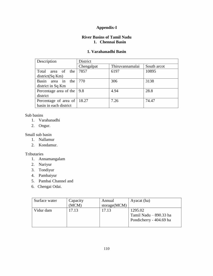
110
Appendix-I
River Basins of Tamil Nadu
1. Chennai Basin
1. Varahanadhi Basin
Description District
Chengalpat Thiruvannamalai South arcot
Total area of the
district(Sq Km)
7857 6197 10895
Basin area in the
district in Sq Km
770 306 3138
Percentage area of the
district
9.8 4.94 28.8
Percentage of area of
basin in each district
18.27 7.26 74.47
Sub basins
1. Varahanadhi
2. Ongur.
Small sub basin
1. Nallamur
2. Kondamur.
Tributaries
1. Annamangalam
2. Nariyur
3. Tondiyur
4. Pambaiyur
5. Pambai Channel and
6. Chengai Odai.
Surface water Capacity
(MCM)
Annual
storage(MCM)
Ayacat (ha)
Vidur dam 17.13 17.13 1295.02
Tamil Nadu – 890.33 ha
Pondicherry - 404.69 ha
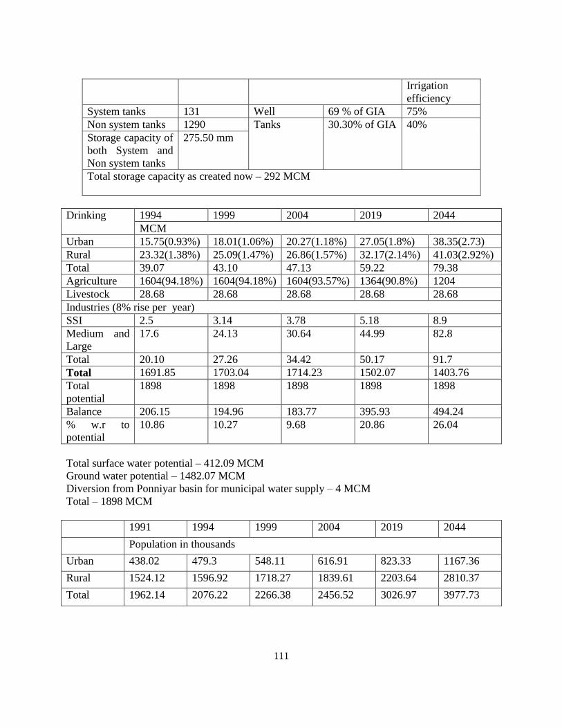
111
Irrigation
efficiency
System tanks 131 Well 69 % of GIA 75%
Non system tanks 1290 Tanks 30.30% of GIA 40%
Storage capacity of
both System and
Non system tanks
275.50 mm
Total storage capacity as created now – 292 MCM
Drinking 1994 1999 2004 2019 2044
MCM
Urban 15.75(0.93%) 18.01(1.06%) 20.27(1.18%) 27.05(1.8%) 38.35(2.73)
Rural 23.32(1.38%) 25.09(1.47%) 26.86(1.57%) 32.17(2.14%) 41.03(2.92%)
Total 39.07 43.10 47.13 59.22 79.38
Agriculture 1604(94.18%) 1604(94.18%) 1604(93.57%) 1364(90.8%) 1204
Livestock 28.68 28.68 28.68 28.68 28.68
Industries (8% rise per year)
SSI 2.5 3.14 3.78 5.18 8.9
Medium and
Large
17.6 24.13 30.64 44.99 82.8
Total 20.10 27.26 34.42 50.17 91.7
Total 1691.85 1703.04 1714.23 1502.07 1403.76
Total
potential
1898 1898 1898 1898 1898
Balance 206.15 194.96 183.77 395.93 494.24
% w.r to
potential
10.86 10.27 9.68 20.86 26.04
Total surface water potential – 412.09 MCM
Ground water potential – 1482.07 MCM
Diversion from Ponniyar basin for municipal water supply – 4 MCM
Total – 1898 MCM
1991 1994 1999 2004 2019 2044
Population in thousands
Urban 438.02 479.3 548.11 616.91 823.33 1167.36
Rural 1524.12 1596.92 1718.27 1839.61 2203.64 2810.37
Total 1962.14 2076.22 2266.38 2456.52 3026.97 3977.73

112
2. Vaippar basin
Kamarajar Madurai Nellai
kattabomman
V.O.
Chidambaranar
Percentage 68 7 5 22
Area 3660.53 352.50 244.03 1165.94
Total area of the basin – 5423 Sq Km.
Tributaries
1. Nichabanadhi
2. Uppodai
3. Kalingalur
4. Arjuna Nadhi
5. Nagariar
6. Kousiga Nadhi
7. Deviar
8. Senkottaiar
9. Kayalkudiar
10. Vallampatti Odai
11. Sevalaperiyar
12. Uppathur
13. Sindapalli.
Irrigation sources
Particulars Ha
Canal 476 (0.16%)
Tank 33077 (11.2%)
Well 64010 (21.68%)
S.No Name of the dam
/reservoir
Capacity in
MCM
Annual storage Ayacat in ha
1 Periyar dam 5.45 10.9 3652
2 Kovilar dam 3.77 7.54 -
3 Vembakottai reservoir 11.29 22.58 3280
4 Kullur sandai reservoir 3.59 7.18 1170
5 Anaikuttam reservoir 3.56 7.12 1214
6 Golwarpatty reservoir 5.20 10.40 1821
Sub total 32.86 65.72 11137
7 Irukkankudi reservoir 14.14 28.28 3787
8 Ullar reservoir 7.73 12.14 4694
Sub total 21.87 40.42 8481
Total 54.73 106.14 19618
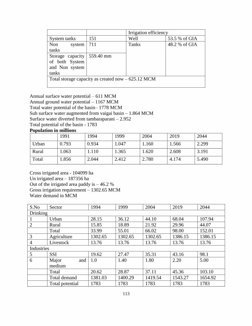
113
Irrigation efficiency
System tanks 151 Well 53.5 % of GIA
Non system
tanks
711 Tanks 48.2 % of GIA
Storage capacity
of both System
and Non system
tanks
559.40 mm
Total storage capacity as created now – 625.12 MCM
Annual surface water potential – 611 MCM
Annual ground water potential – 1167 MCM
Total water potential of the basin– 1778 MCM
Sub surface water augmented from vaigai basin – 1.864 MCM
Surface water diverted from tambaraparani – 2.952
Total potential of the basin - 1783
Population in millions
1991 1994 1999 2004 2019 2044
Urban 0.793 0.934 1.047 1.160 1.566 2.299
Rural 1.063 1.110 1.365 1.620 2.608 3.191
Total 1.856 2.044 2.412 2.780 4.174 5.490
Cross irrigated area - 104099 ha
Un irrigated area – 187356 ha
Out of the irrigated area paddy is – 46.2 %
Gross irrigation requirement – 1302.65 MCM
Water demand in MCM
S.No Sector 1994 1999 2004 2019 2044
Drinking
1 Urban 28.15 36.12 44.10 68.04 107.94
2 Rural 15.85 18.89 21.92 29.96 44.07
Total 33.99 55.01 66.02 98.00 152.01
3 Agriculture 1302.65 1302.65 1302.65 1386.15 1386.15
4 Livestock 13.76 13.76 13.76 13.76 13.76
Industries
5 SSI 19.62 27.47 35.31 43.16 98.1
6 Major and
medium
1.0 1.40 1.80 2.20 5.00
Total 20.62 28.87 37.11 45.36 103.10
Total demand 1381.03 1400.29 1419.54 1543.27 1654.92
Total potential 1783 1783 1783 1783 1783
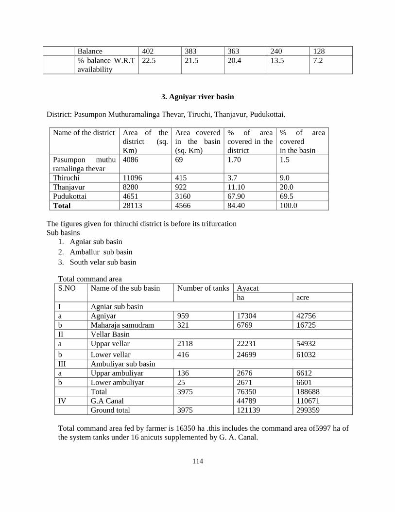
114
Balance 402 383 363 240 128
% balance W.R.T
availability
22.5 21.5 20.4 13.5 7.2
3. Agniyar river basin
District: Pasumpon Muthuramalinga Thevar, Tiruchi, Thanjavur, Pudukottai.
Name of the district Area of the
district (sq.
Km)
Area covered
in the basin
(sq. Km)
% of area
covered in the
district
% of area
covered
in the basin
Pasumpon muthu
ramalinga thevar
4086 69 1.70 1.5
Thiruchi 11096 415 3.7 9.0
Thanjavur 8280 922 11.10 20.0
Pudukottai 4651 3160 67.90 69.5
Total 28113 4566 84.40 100.0
The figures given for thiruchi district is before its trifurcation
Sub basins
1. Agniar sub basin
2. Amballur sub basin
3. South velar sub basin
Total command area
S.NO Name of the sub basin Number of tanks Ayacat
ha acre
I Agniar sub basin
a Agniyar 959 17304 42756
b Maharaja samudram 321 6769 16725
II Vellar Basin
a Uppar vellar 2118 22231 54932
b Lower vellar 416 24699 61032
III Ambuliyar sub basin
a Uppar ambuliyar 136 2676 6612
b Lower ambuliyar 25 2671 6601
Total 3975 76350 188688
IV G.A Canal 44789 110671
Ground total 3975 121139 299359
Total command area fed by farmer is 16350 ha .this includes the command area of5997 ha of
the system tanks under 16 anicuts supplemented by G. A. Canal.

115
Agniyar river basins consists of 3 sub basins i.e ) agniyar, ambuliyur and south velar.
There are seven tributaries in the basin. The river agniyar have three tributaries viz., nariar I,
nariar II and maharaja samudram. The river ambuliyur have two tributaries viz., punakuttiyar
and Maruthangudiyarthe River south vellar have two tributaries viz., nerunjikudiar and
gundar. There are three gauging station in agniyar river basin managed by public work
department.
1. Poovanam anicut- agniyar
2. Adaiklladevan anicut –ambuliyar
3. Manamelkudi anicut –south vellaran important point to be noted in this basin is that there
are no reservoirs across any of the rivers of the basin. The main reason being none of the
rivers have copious flow.the terrain of the country is also ------- and it is difficult to
construct any reservoir. There is no dual ayacat fed by the rivers of the basin. There are
about 3975 tanks in the basin by which 76350 ha are being irrigated out of the above 346
are system tanks and 3629 are non-system tanks. The approximate storage capacity of
these tanks is 560 MCM.
Surface Water Potential
The total SWP for 15% probability for agniyar river basin is as follows
1. South west monsoon surface Water Potential – 222 MCM
2. North east monsoon surface Water Potential – 239 MCM
3. Annaur surface Water Potential – 585 MCM
Total surface water potential
1. Surface water potential generated within the basin I – 585 MCM
2. Surface water quantity diverted from Cauvery river - 499 MCM
Total - 1084 MCM
The total water potential of the agniyar
Surface water potential – 585 MCM
Diversion from Cauvery basin through G.A canal – 499 MCM
Total surface water potential – 1084 MCM
Ground water potential – 920 MCM

116
Total water potential – 1084 +920 -2004 MCM
Population
Year 1994 1999 2004 2019 2044
Urban 0.282 0.307 0.331 0.404 0.526
Rural 1.255 1.333 1.411 1.645 2.035
Total 1.537 1.640 1.742 2.049 2.561
Present and future water demand (in MCM)
Sector 1991 1994 1999 2004 2019 2044
Agriculture - 2344.00 2344.00 2344.00 2344.00 2344.00
Domestic
Urban 8.80 9.28 10.08 10.87 13.27 17.27
Rural 17.65 18.33 19.47 20.61 24.02 29.71
Sub total 26.45 27.61 29.55 31.48 37.29 46.98
Livestock - 14.80 14.80 14.80 14.80 14.80
Industries
Small - 1.47 2.06 2.65 4.41 7.35
Major and
medium
- 15.62 21.87 28.12 46.86 78.10
Sub total - 17.09 23.93 30.77 51.27 85.45
Total 52.90 2403.50 2412.28 2421.05 2447.36 2491.23
Water balance
Year Present Short term Long term
1994 1999 2004 2019 2044
Total demand 2404 2412 2421 2447 2491
Total potential 2004 2004 2004 2004 2004
Deficit 400 408 417 443 487
% of deficit
w.r to demand
16.6 16.9 17.2 18.1 19.6
Short term:
In the short term period ending 2004 the water deficit is in the order of 16.9 % to 17.2 %
Long term:
In the Long term period ending 2044 water deficit is in the order of 18.1 % to 19.6 %

117
4. Pambar and kottakaraiyar basin
S.No Name of the district Area of the
district in Sq. Km
Area covered by
this basin in Sq.
Km
% area covered
by this basin
1 Dindugal –mannar
thirumalai
6058 478 7.89
2 Tiruchy –
perumpidugu
mutharaiyar
11096 44 0.40
3 Pudukottai 4651 809 17.39
4 Pasumpon -
muthuramalingam
4086 2989 73.15
5 Madurai 6565 279 4.25
6 Ramanathapuram 4232 1248 29.49
Three streams
1. Koluvanaru
2. Pambar
3. Kottakaraiyar. Cropping pattern and cropping calendar
S.No First crop Season
1 Paddy Aug –Jan to Oct -Feb
2 Cholam Mar – May
3 Ragi Mar – June
4 Chillies Dec –Apr
5 Gingelly Dec- Mar
6 Cotton Feb –July
7 Sunflower Jan -May
Groundnut Jan – Apr
Total ayacat irrigated – 13204 ha
Tanks – 1161
Surface water potential -653 MCM
Ground water potential – 976 MCM
Total water potential – 1629 MCM
Population in millions
Sector 1994 1999 2004 2019 2044
Urban 0.439 0.472 0.505 0.604 0.769
Rural 1.281 1.350 1.420 1.627 1.972
Total 1.720 1.822 1.925 2.231 2.741

118
Present and future demand
Sectors 1994 1999 2004 2019 2044
Domestic
Urban 14.41 15.49 16.58 19.85 25.28
Rural 18.71 19.72 20.73 23.75 28.79
Total 33.12 35.21 37.31 43.60 54.07
Agriculture 1960.73 1960.73 1960.73 1960.73 1960.73
Livestock 24.98 24.98 24.98 24.98 24.98
Industries
SSI 4.04 5.66 7.27 12.12 20.20
Large and
medium
30.55 41.87 53.19 87.13 143.71
Total 34.59 47.53 60.46 99.25 163.91
Total demand 2053.42 2068.45 2083.48 2128.56 2203.69
Water
potential
1629 1629 1629 1629 1629
Deficit 424 439 454 500 575
Deficit % 26.03 26.95 27.87 30.69 35.30
5. Nambiyar basin
District Total area in Sq Km Basin area in Sq km % of th district area
V.O. Chidambaranar 4621 520 11.26
Tirunelveli
kattabomman
6810 1464 21.49
Kanyakumari 1685 100 5.94
Sub basin:
1. Karumaniyar
2. Hanumanadhi
3. Pachaiyar
4. manimuthar canal
5. Nambiyar River
Tributaries
1. Thamarayar
2. Parattayar

119
Name of the
reservoir
Capacity in
MCM
Annual storage
in MCM
Ayacat in ha
Nambiyar 2.33 2.59 705.65
Kodumudiyar 3.58 7.56 2340.00
System tanks- 559
Non System tanks – 38
Approximate storage capacity of these tanks – 94.54 MCM
Total storage capacity as created now -100.45 MCM
Surface water potential - 203.87 MCM
Annual ground water potential – 274.74 MCM
Total water potential – 478.61 MCM
Basin GIA – 3365
Present and future water demand
Sector 1994 1999 2004 2019 2044
Domestic use
Urban 4.40(0.81) 4.80(0.82) 5.26(0.90) 6.54(0.10) 8.67(1.44)
Rural 6.24(1.15) 6.94(1.18) 7.65(1.30) 9.77(1.65) 13.31(2.21)
10.64 11.74 12.91 16.31 21.98
Agriculture 523.59(96.7) 566(96.63) 566(96.32) 566(95.41) 566(93.93)
Livestock 5.42(1.00) 5.42(0.93) 5.42(0.92) 5.42(0.91) 5.42(0.90)
Industries 1.83(0.34) 2.56(0.44) 3.29(0.56) 5.49(0.93) 9.15(1.52)
Total 541.48 585.72 587.62 593.22 602.55
Potential 478.61 478.61 478.61 478.61 478.61
Surflus /
deficit
-62.87 -107.11 -109.01 -114.61 --123.94
Percentage of
total dd
-11.61 -18.29 -18.55 -19.32 -20.57
Population (in millions)
Sector 1994 1999 2004 2019 2044
Urban 0.134 0.146 0.160 0.199 0.264
Rural 0.427 0.475 0.524 0.669 0.991
Total 0.561 0.621 0.684 0.868 1.155

120
6. Palar river basin
Name of the district Area falling in the basin
Vellore (north arcot- ambedkar) 4710.58
Thiruvannamalai (Thiruvannamalai-
sambuvarayar)
4012.19
Kancheepuram (chengai MGR) 2187.90
Total 10910.67
Tributaries
1. Poiney
2. Kaudinganadhi
3. Malattar
4. Cheyyar
5. Agaramar
6. Killiyur
7. Vegavathiar
Name of the basin
1. Uppar palar
2. Kamandala naganadhi
3. Upper cheyyar
4. Kilya palar
5. Lower palar
Surface water
Dams and reservoir
The river palar is having 5 tributaries namely poiney, Kaudinganadhi, Malattar, Cheyyar
Killiyur. Flow measurement is being taken in 7 locations namely 1. Palar anicut 2. Poiney 3.
Aliabad 4. Kamandalanaganadhi 5.cheyyar 6. Tandalai and 7. Uthiramerur. Apart from the 4
gauge are maintained by central water commission.hey are avarakuppam, magaral, arcot and
chengalpattu. There is no major reservoir in the basin. However, there is two reservoir under
construction in the basin namely marthana andrajathoppu canal.
There are about 661 system tanks by which 60972 ha are being irrigated. The storage
capacity of these tanks is approximately355 MCM and total storage capacity as created now
is 355 MCM (approximately) only.

121
Population (in millions)
Area 1994 1999 2004 2019 2044
Urban 1.611 1.834 2.057 2.725 3.839
Rural 3.630 3.878 4.126 4.870 6.110
Total 5.241 5.712 6.183 7.595 9.949
Present and future water demand
Sector 1994 1999 2004 2019 2044
Domestic use
Urban 52.95 60.26 67.58 89.53 126.12
Rural 53 56.62 60.24 71.11 89.21
105.95 116.88 127.82 160.67 215.33
Livestock 60.09 60.09 60.09 60.09 60.09
Industries
SSI 4.47 5.32 6.16 8.69 12.91
Large and
medium
8.63 49.66 60.70 93.81 148.99
Total 43.10 54.98 66.86 102.5 161.9
Atomic
power
5.00 10.00 10.00 10.00 10.00
Total 2746.14 273.95 2796.77 2865.23 2979.36
Demand prediction
The future requirement has been assessed based on the information received from SG &
SWRDE (ground water department) of WRO and is 100 MCM per year. Thus the future
water demand computed as fallows.
Particulars Water requirements in MCM
1994 1999 2004 2019 2044
Atomic power
plant at kalpakkam
5.00 10.00 10.00 10.00 10.00
Water balance
The total surface water potential of the palar basin works out to 1758.00 MCM of the
ground waater potential of the palar basin works out to 2160.32 MCM.
Surface water potential of the basin -1758.00 MCM
Ground water potential of the basin – 2610.32
Total water potential of the basin – 4368.32

122
Year 1994 1999 2004 219 2044
Total water
potential of the
basin(MCM)
4368.32 4368.32 4368.32 4368.32 4368.32
Total water
demand(MCM)
2746.14 2773.95 2796.77 2865.23 2979.36
Balance water
(MCM)
1622.18 1594.37 1571.55 1403.09 1388.96
% of surplus 37 36 36 32 32
Short term
In general in the ST period ending 2004, the water balance of the basin varies from
1622.18 to 1571.55 MCM.
Long term
In long term period ending 2044, the water balance of the basin decreases from 1403.09
to 1388.96 MCM.
7. Ponnaiyar river basin
District: Dharmapuri, North –Arcot, Thiruvannamalai, South Arcot, Villupuram
S.No Name of the
District
Total Area of
the District
Area of the
basin falling
in the dt
% Area of the
dt falling in
the basin
% Area of
basin falling
in the dt
1. Dharmapuri 9622 6744.03 70.10 59.91
2. N.Arcot-
ambedkhar &
thiruvannamalai
- sambuvarayar
12268 1315.31 10.72 11.68
3. S.Arcot-vallalar
and Villupuram
– ramasamy
padiyachiyar
10894.00 3197.66 29.35 28.41
Ponnaiyar River is having 10 tributaries namely,
1. Chinnar I
2. Chinnar II
3. Markandandhi
4. Pullam pattinadhi
5. Pambar
6. Vaniar
7. Kallar
8. Pambanar
9. Musukundanadhi
10. Thurinjalar

123
Name of the Reservoir:
1. Krishnagiri
2. Sathanur
3. Pambar
4. Shoolagirichinnur
5. Vaniar
6. Thumbalahalli
7. Kelavarapalli
Irrigated Area – 650 Sq.km
Unirrigated Area – 2975 Sq.km
Dry Farm – 287 Sq.km
No Storage Capacity
System Tanks 1133 119
Non-System Tanks 0 121
Total 240
Total Capacity of Reservoir – 311.00
Area cut in Ha – 32172
Total Storage Capacity as created now – 311 + 240 = 551 mcm
System Tank – 304, Ayacut – 26133
Non-System Tank – 829, Ayacut – 18673
Direct area cut of this basin – 46010
Total ayacut of basin – 90806
Surface Water Potencial: 1310.43 mcm
Ground water - 1560
Total Water Potencial: 2870 mcm
s.no crop Season Net crop water
requirement
1 Paddy Aug –jan
Feb –june
Oct -mar
655.00
1005.00
92.00
2 Groundnut July –oct
Nov-mar
453.00
320.00
3 Sugarcane feb -jan 1300.00
4 Sorghum -bajra Jan -mar 318.00
5 Ragi & other millets - 405.50

124
Irrigation requirement
Present & Future Demand in mcm
S.No Sector 1994 1999 2004 2019 2044
1. Domestic
a) Urban 19.34 21.06 22.77 27.90 36.48
b) Rural 49.46 53.03 57.79 72.69 95.87
Subtotal 68.81 74.69 80.56 99.99 132.35
2. Agriculture 2668.8 2668.8 2668.8 2321.39 2089.78
3. Livestock 53.84 53.84 53.84 53.84 53.84
4. Industries
a) Small scale 6.52 9.13 11.74 19.56 32.60
b) Large scale 63.07 86.43 109.79 179.87 296.67
Subtotal 69.59 95.56 121.53 199.43 329.27
Total 2861.04 2892.89 2924.73 2674.65 2605.24
For demand computed based on the strategy of 1351 pcd per person in urban area and 70
Lpcd per person in rural area, the demand will be shown in the following table,
S.No Sector 1994 1999 2004 2019 2044
1. Domestic
a) Urban 27.90 30.38 32.85 40.29 52.68
b) Rural 86.55 92.80 99.05 117.80 149.05
Subtotal 114.45 123.18 131.09 158.09 201.73
2. Agri 2668.80 2668.80 2668.80 2321.39 2089.78
3. Livestock 53.84 53.84 53.84 53.84 53.84
4. Industrial
a) Small scale 6.52 9.13 11.74 19.56 32.60
b) Large sclae 63.07 86.43 109.79 179.87 296.67
Subtotal 69.59 95.56 121.53 199.43 329.27
Total 2986.68 2941.38 2976.07 2732.75 2674.62
Crop Area in ha Net crop water
requirement mm
System area
Paddy 23973 206.80
Groundnut 13981 63.45
Ragi 12433 50.45
Sugarcane 5820 75.66
Total 62227 448.29
Non system area
Paddy (tanks) 28579 246.54
Paddy (others) 41166 355.12
Sugarcane 26436 343.68
Total 412106 945.34

125
Water Balance:
S.No Year 1994 1999 2004 2019 2044
01. Water Potential 2870 2870 2870 2870 2870
Low Projection
02. Water Demand 2861.04 2892.89 2924.73 2674.65 2605.24
03. Balance 8.96 - - 197.16 269.55
04. % Balance
W.R.T
Availability
0.31 - - 6.9 9.4
High Projection
05. Water Demand 2906.68 2941.38 2976.07 2732.75 2674.62
06. Balance - - - 129.21 185.08
07. % Balance
W.R.T
Availability
- - - 4.5 6.4
Gadilam Basin: Ponniyar Basin (Population in millions)
S.No Population 1994 1999 2004 2019 2044
1. Urban 0.589 0.641 0.693 0.850 1.110
2. Rural 3.386 3.673 3.958 4.813 6.238
Total 3.977 4.314 4.651 5.663 7.348
S.No Name of the Reservoir Capacity in mcm Ayacut in Ha
1. Krishnagiri 66.10 3642
2. Sathanur 207.00 1822
3. Pambar 7 1620
4. Shoolagiri Chinnar 2.30 352
5. Vaniar 11.80 4212
6. Thumbalahalli 3.70 884
7. Kelavarapalli (Under
Construction) 13.10 3240
Total 311 32172

126
8. Vellar river basin
S.No District Area of the district
in Sq.km
Area
covered
by vellar
basin
sq.km
% area of the
dist covered
in the basin
% area of the
basin covered
by the dist
1. Dharmapuri 9622 69 0.72 0.90
2. Salem 8649 2439 28.20 31.90
3. Tiruchi 11096 1658 14.94 21.60
4.
Villupuram
Ramasamy
Padayachiyar
6276 1855 29.56 24.30
5. South Arcot 4619 1638 35.46 21.30
Total 7659 100
Dams and Reservoir:
The river vellar is having four main tributaries homely swethanadhi,
manimukthnadhi chinnal and anavarai odai. At 10 places, river flows are measured. They are:
i) Anaimaduvu reservior
ii) Kariyakoil reservior
iii) Gomuki reservior
iv) Manimuthanadhi reservior
v) Willington reservior
vi) Memattur anicuts reservior
vii) Virudhachalam reservior
viii) Tholudur reservior
ix) Relandurai reservior
x) Sethiyathope reservior
S.No Name of the
Reservoir
Gross Capacity in
mcm
Ayacut in Ha
. Anaimadavu 7.56 2118
2. Kariyakoil 8.38 1457
3. Gomuki 15.86 2023
4. Mnaimuktha 20.87 1720
5. Millingdon 65.18 11068
Total 114.85 18386

127
The vellar basin system anicuts in the main river as well as in us tributaries. There are
about 386 system tanks and 71 Non-system tanks. The total crop area of anicuts and tanks are
given below:
S,No Anicuts and Tanks Area in Ha
1. Ayacuts under regulators 5 nos 24580
2. Ayacuts of minor anicuts (215 nos)
including system tanks (386 nos)
21516
3. Ayacuts of non-system tanks (71 nos) 6972
4. Ayacuts of Reservoir (5 nos) 18386
Total 71455
The storage capacity of these tanks and reservoir are 70.00 mcm & 115.00 mcm
respectively. The total storage capacity of these basins as created now is (115.00 & 70.00 = 185
mcm)
Population in millions:
S.No Area 1994 1999 2004 2019 2044
1. Urban 0.767 0.824 0.881 1.051 2.335
2. Rural 2.679 2.867 3.056 3.622 3.565
Total 3.446 3.691 3.937 4.673 5.900
Total SW Potential: 1065
Total GW Potential: 1344
Water diverted received surplus water from veeranm tank of adjoining Cauvery basin: 78 mcm
Water diverted from this basin adjoining paravanar basin: 72 mcm
Total water potential of this basin: 2409 + 78 – 72 = 2415 mcm
Present & Future water demand in mcm:
S.No Sector 1994 1999 2004 2019 2044
1. Domestic
a) Urban 25.20 27.06 28.93 34.53 43.87
b) Rural 39.11 41.86 44.62 52.88 66.65
Sub total 64.31 68.92 73.55 87.41 110.52
2. Agriculture 2229.26 2229.26 2229.26 1946.25 1759.47
3. Livestock 51.17 51.17 51.17 51.17 51.17

128
4. Industries
a) Small scale 8.42 11.79 15.16 25.96 42.10
b) Large scale 24.63 33.76 42.88 70.25 115.87
Subtotal 33.05 45.55 58.04 96.21 157.92
Total 2377.79 2394.9 2415.02 2181.04 2079.13
For the demand computed based on the strategy of 135 lpcd per person in urban area &
70 lpcd per person in rural area, the demand will be as shown in the following table.
S.No Sector 1994 1999 2004 2019 2044
1. Domestic
a) Urban 37.80 40.59 43.40 51.80 65.81
b) Rural 68.44 73.26 78.09 92.54 116.64
Sub total 106.24 113.85 121.49 144.34 182.45
2. Agriculture 2229.26 2229.26 2229.26 1946.25 1759.47
3. livestock 51.17 51.17 51.17 51.17 51.17
4. industries
5. Small sector 8.42 11.79 15.16 25.96 42.10
6. Large sector 24.63 33.76 42.88 70.25 115.87
Sub total 33.05 45.55 58.04 96.21 157.97
Total 2419.72 2439.83 2459.96 2237.97 2151.06
Water balance: the total water potential of vellar basin mt 2415 mcm
S.No Year 1994 1999 2004 2019 2044
1. Water potential 2415.00 2415.00 2415.00 2415.00 2415.00
Low Projection
2. Water Demand 2377.79 2394.90 2412.02 2181.04 2079.13
3. Balance 37.21 20.10 2.98 233.96 335.87
4. % Balance WRT
Availability 1.5 0.8 0.1 9.7 13.9
High Projection
5. Water Demand 2419.72 2439.83 2459.96 2237.97 2151.06
6. Balance - 4.72 -24.83 -44.96 177.03 263.94
7. % Balance WRT
Availability - - - 7.3 10.9

129
Surface water potential: The annual surface water potential for 95%, 75%, 50% probability has
been assessed for vellar river basin and they are given below:
1. Annual surface water potential for 95% probability – 789326 mcm
2. Annual surface water potential for 75% probability – 962.74 mcm
3. Annual surface water potential for 50% probability – 1064.98 mcm
4. Annual ground water potential – 1344 mcm
5. Total water potential – 1065 + 1344 = 2409.26 mcm
Total water potential:
The annual total water resource potential of this basin is (SW at 75% dependability =
1065 mcm + GW = 1344 mcm = 2409.26 mcm) this basin also receives surplus water of veeranam
tank of adjoining Cauvery basin at sethiathope anicuts. It has been roughly estimated as 78
mcm/annum. Water is also diverting from thus basin to the adjoining paravanar basin to wallajab
tank through vellar. Rajan channel is about 72.0 mcm per annum. Thus the total water potential of
thus basin is 2409 + 78 – 72 = 2415 mcm.
Existing management system:
These are 386 tanks both system and Non-system tanks. They irrigate about 11999 Ha and
the 5 reservoir in the vellar basin irrigate about 18386 ha.
Competing water demand
In vellar river basin crop area of 74106 ha are irrigated by reservoirs, system and non system
tanks. For this area, an efficiency of 40% is adopted. An extent of 68658 ha is irrigated by wells.
The efficiency for well irrigation is considered as 75% crop water requirement is computed using
the crop.
9. Kodaiyar river basin
Districts: western Ghats of kanyakumari
Basic area -1553 SSq Km
Name of the dame /reservoir
1. Pechiparai dam
2. Perunchani dam
3. Chittar dam I
4. Kodaiyar dam I
5. Kodaiyar dam II
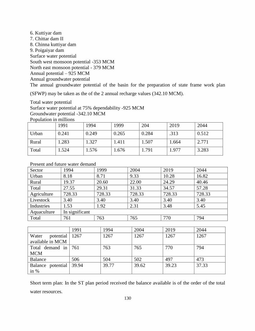
130
6. Kuttiyar dam
7. Chittar dam II
8. Chinna kuttiyar dam
9. Poigaiyar dam
Surface water potential
South west monsoon potential -353 MCM
North east monsoon potential - 379 MCM
Annual potential – 925 MCM
Annual groundwater potential
The annual groundwater potential of the basin for the preparation of state frame work plan
(SFWP) may be taken as the of the 2 annual recharge values (342.10 MCM).
Total water potential
Surface water potential at 75% dependability -925 MCM
Groundwater potential -342.10 MCM
Population in millions
1991 1994 1999 204 2019 2044
Urban 0.241 0.249 0.265 0.284 .313 0.512
Rural 1.283 1.327 1.411 1.507 1.664 2.771
Total 1.524 1.576 1.676 1.791 1.977 3.283
Present and future water demand
Sector 1994 1999 2004 2019 2044
Urban 8.18 8.71 9.33 10.28 16.82
Rural 19.37 20.60 22.00 24.29 40.46
Total 27.55 29.31 31.33 34.57 57.28
Agriculture 728.33 728.33 728.33 728.33 728.33
Livestock 3.40 3.40 3.40 3.40 3.40
Industries 1.53 1.92 2.31 3.48 5.45
Aquaculture In significant
Total 761 763 765 770 794
1991 1994 2004 2019 2044
Water potential
available in MCM
1267 1267 1267 1267 1267
Total demand in
MCM
761 763 765 770 794
Balance 506 504 502 497 473
Balance potential
in %
39.94 39.77 39.62 39.23 37.33
Short term plan: In the ST plan period received the balance available is of the order of the total
water resources.

131
Long term plan: In the LT plan period the balance potential available ranges from 37.33 to 39.23
Reservoirs
S.No Name of the dam Capacity MCM Annual storage
MCM
Ayacut area in ha
1 Pechiparai dam 152.36 152.36
2 Perunchani dam 81.84 81.84
3 Chittar dam I 17.28 17.28 Combined
ayacutof
kodaiyar is
36836
4 Chittar dam II 28.25 28.25
5 Kodaiyar dam I 118.50 118.50
6 Kodaiyar dam II 0.883 0.883
7 Kuttiyar dam 0.222 0.222
8 Chinna kuttiyar dam 2.776 2.776
9 Poigaiyar dam
Total
2.700
405.116
2.700
Out of the above 9 reservoirs the first and last reservoir are under the control of PWD &
the other are under the control of TN electricity board.there are 2922 tanks by which 46024 ha
are being irrigated out of the above 1462 are system tanks and 1460 are non system tanks . The
approximate storage of these tanks is 268 MCM .the total storage capacity of the basin as created
now is 673 MCM.
.10. Kallar river basin
Total basin area – 1878.80 Sq Km. 40.66% of the district out of 4621 Sq Km is covered by the
basin.
Sub basin:
1. Kallar
2. Korampallamaru.
Kallar is having 3 tributaries (joining with uppar odai) viz. left arm of uppar odai,
Chekarakudi River and Perurani River. There are no tributaries for Korampallamaru River.
Tributaries – uppar odai
1. Left arm of uppar odai
2. Chekarakudi river
3. Perurani river
Name of the
dam/reservoir
capacity Annual storage Ayacut area in ha
Eppothumventran 3.57 4.91 421
Cropping pattern and crop calendar

132
Crop 1st season 2
nd season 3
rd season
Paddy Pishanam Paddy Navarai (feb –jan )
Paddy (sornavari) Pishanam Paddy Sornavari (apr -july)
Un irrigated crop
Cotton/pulses
Cotton/vegetables
(sep- oct,feb-mar) - -
Pulses sep- oct,nov-dec) - -
Cholam sep- oct,dec- jan) - -
Sunflower Perennial - -
Surface water potential
South west monsoon – 12.96 MCM
Narth east monsoon – 66.79 MCM
Annual – 124.56 MCM
Diversion from thabarabarani basin for irrigation -6.59 MCM
The utilizable ground water recharge, draft and balance of potential of kallar basin have been
estimated as 69.58 MCM, 26.94 MCM & 42.64 MCM / yr respectively.
Population in millions
1994 1999 204 2019 2044
Urban 0.253 0.267 0.282 0.326 0.400
Rural 0.353 0.362 0.370 0.396 0.440
Total 0.606 0.629 0.652 0.722 0.840
Present and future water demand
Sector 1994 1999 2004 2019 2044
Urban 8.30
4.01
8.78
4.12
9.27
4.14
10.72
4.42
13.15
4.82
Rural 5.16
2.49
5.28
2.48
5.41
2.41
5.79
2.39
6.42
2.35
Total 13.46 14.06 14.68 16.51 19.57
Agriculture 167.00
80.67
167.00
78.37
167.00
74.49
167.00
68.88
167.00
61.19
Livestock 0.90
0.43
0.90
0.42
0.90
0.40
0.90
0.37
0.90
0.33
Industries 14.88
7.19
20.35
9.55
25.84
11.53
42.28
17.44
69.68
25.53
SSI 0.28 0.35 0.42 0.64 1.06
Large &
medium
14.60 20.00 25.42 41.64 68.68
Power 10.78
5.20
10.78
5.06
15.76
7.03
15.76
6.50
15.76
5.78
Total 207.02 213.09 224.18 242.45 272.92
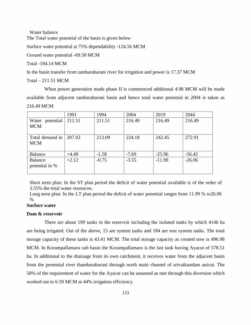
133
Water balance
The Total water potential of the basin is given below
Surface water potential at 75% dependability -124.56 MCM
Ground water potential -69.58 MCM
Total -194.14 MCM
In the basin transfer from tambarabarani river for irrigation and power is 17.37 MCM
Total – 211.51 MCM
When power generation made phase II is commenced additional 4.98 MCM will be made
available from adjacent tambarabarani basin and hence total water potential in 2004 is taken as
216.49 MCM
1991 1994 2004 2019 2044
Water potential
MCM
211.51 211.51 216.49 216.49 216.49
Total demand in
MCM
207.02 213.09 224.18 242.45 272.91
Balance +4.49 -1.58 -7.69 -25.96 -56.42
Balance
potential in %
+2.12 -0.75 -3.55 -11.99 -26.06
Short term plan: In the ST plan period the deficit of water potential available is of the order of
3.55% the total water resources.
Long term plan: In the LT plan period the deficit of water potential ranges from 11.99 % to26.06
%
Surface water
Dam & reservoir
There are about 199 tanks in the reservoir including the isolated tanks by which 4146 ha
are being irrigated. Out of the above, 15 are system tanks and 184 are non system tanks. The total
storage capacity of these tanks is 43.41 MCM. The total storage capacity as created now is 496.98
MCM. In Korampallamaru sub basin the Korampallamaru is the last tank having Ayacut of 578.51
ha. In additional to the drainage from its own catchment, it receives water from the adjacent basin
from the perennial river thambarabarani through north main channel of srivaikundam anicut. The
50% of the requirement of water for the Ayacut can be assumed as met through this diversion which
worked out to 6.59 MCM at 44% irrigation efficiency.

134
1. Chennai basin
The details of the district and its area that come under this basin are
S.No District District area
in SqKm
District area
falling in the
basin (Sq Km)
Percentage of
area in the
basin
Percentage of
district area
in the basin
1 Chennai 174 174 100 3.1
2 Chengai - MGR 7857 4275 54.4 77.1
3 North arcot 6077 1093 17.98 19.8
The Chengai – MGR District referred is undivided district
Details of area of each sub basin
S.No Name of the sub basin Area of the sub basin
1 Araniyar 763
2 Kusaimalaiyar 3240
3 Cooum 682
4 Adayar 857
Total 5542
The direct ayacut - 115479 ha
1304 tanks – 85208
215 – 21000 -indirect Ayacut
The storage capacity of the exisisting reservoir – 320.0 MCM
Well irrigation -46. 5%
Tank irrigation – 42.2%
Storage capacity of tanks – 619 MCM
Total storage capacity as created now -939.0 MCM
Total surface water potential -906.00 MCM
Year 1991 1994 1999 2004 2019 2044
Urban 169.18 181.43 201.85 222.27 283.52 380.61
Rural 25.81 27.02 29.02 31.05 37.1 47.18
Total 194.99 208.85 230.88 253.32 320.62 432.79
Present and future water demand
Sector 1994 1999 2004 2019 2044
Domestic 208.45 230.88 253.32 320.62 432.79
Agriculture 2864.7 2864.7 2864.7 2508.0 2393.0
Livestock 38 38 38 38 38
Industries
Small, large
& medium
86.23 120.72 155.25 258.69 431.15
Recreation 28.00 28.00 28.00 28.00 28.00
Power 3.32 22.40 23.00 25.00 30.00
Total 3228.7 3304.7 3362.27 3252.31 3352.94

135
Water balance
Surface water potential for the year 1994
Total Surface water potential in Chennai basin -784.00 MCM
Diversion from palar basin – 122.00 MCM
Total water potential in 1994 is
Surface water 906.00+ ground water 112.22 – 2026.22 MCM
Total ground water potential as per ground water estimation committee norms-1119.39 MCM
Ground water drawn from palar through filtration wells – 0.83 MCM
Total – 1120.22 MCM
Year 1994 1999 2004 2019 2044
Total water
potential
2026.22 2026.8 2431.22 2431.22 2431.22
Total water
demand in
MCM
3228.70 3304.70 3362.27 3252.31 3352.94
Water deficit
in MCM
-1202.48 1277.90 -931.05 -821.09 -921.02
Water deficit
%
37.24 63.05 38.29 33.77 37.91
Surface water potential expected
Diversion expected from Krishna water – 340.00 MCM
Diversion expected from veeranam tank – 65 MCM
Name of the dam /
reservoir
Capacity in MCM( raised by 0.61 m) Ayacut in ha
Before raising F.R.L After raising F.R.L
Pondi
(sathyamoorthy)
77.96 97.98 -
Red hills 80.71 93.46 -
Cholavaram 25.63 25.30 -
Chembarabakkam 88.36 103.23 5452
11. Paravanar basin
Name of the
taluk
Name of block Area In Sq.km
Panrutti Panrutti 60
Cuddalore Cuddalore 15
Kurinjipadi 345
Vridhachalam Kammapuram 120
Chidambaram parengipettai 75
Mel buvanagin 145
Total basin area 760
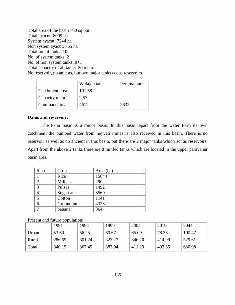
136
Total area of the basin 760 sq. km
Total ayacut: 8009 ha
System ayacut: 7244 ha
Non system ayacut: 765 ha
Total no. of tanks: 10
No. of system tanks: 2
No. of non system tanks: 8+1
Total capacity of all tanks: 20 mcm.
No reservoir, no anicuts, but two major tanks act as reservoirs.
Walajah tank Perumal tank
Catchment area 191.58
Capacity mcm 2.57
Command area 4612 2632
Dams and reservoir:
The Palar basin is a minor basin. In this basin, apart from the water form its own
catchment the pumped water from neyveli mines is also received in this basin. There is no
reservoir as well as no ancient in this basin, but there are 2 major tanks which act as reservoirs.
Apart from the above 2 tanks there are 8 rainfed tanks which are located in the upper paravanar
basin area.
S.no Crop Area (ha)
1 Rice 15844
2 Millets 290
3 Pulses 1492
4 Sugarcane 3560
5 Cotton 1141
6 Groundnut 4323
7 banana 364
Present and future population:
1991 1994 1999 2004 2019 2044
Urban 53.60 56.25 60.67 65.09 78.36 100.47
Rural 286.59 301.24 323.27 346.20 414.99 529.61
Total 340.19 367.49 383.94 411.29 493.35 630.08
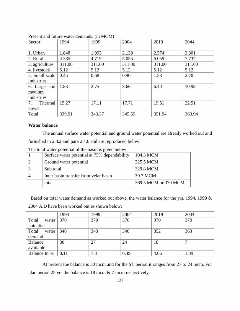
137
Present and future water demands: (in MCM)
Sector
1994 1999 2004 2019 2044
1. Urban 1.848 1.993 2.138 2.574 3.301
2. Rural 4.385 4.719 5.055 6.059 7.732
3. agriculture 311.00 311.00 311.00 311.00 311.00
4. livestock 5.12 5.12 5.12 5.12 5.12
5. Small scale
industries
0.45 0.68 0.90 1.58 2.70
6. Large and
medium
industries
1.83 2.75 3.66 6.40 10.98
7. Thermal
power
15.27 17.11 17.71 19.51 22.51
Total 339.91 343.37 345.59 351.94 363.94
Water balance
The annual surface water potential and ground water potential are already worked out and
furnished in 2.3.2 and para 2.4.6 and are reproduced below.
The total water potential of the basin is given below:
1 Surface water potential at 75% dependability 104.3 MCM
2 Ground water potential 225.5 MCM
3 Sub total 329.8 MCM
4 Inter basin transfer from velar basin 39.7 MCM
total 369.5 MCM or 370 MCM
Based on total water demand as worked out above, the water balance for the yrs, 1994, 1999 &
2004 A.D have been worked out as shown below:
1994 1999 2004 2019 2044
Total water
potential
370 370 370 370 370
Total water
demand
340 343 346 352 363
Balance
available
30 27 24 18 7
Balance In % 8.11 7.3 6.49 4.86 1.89
At present the balance is 30 mcm and for the ST period it ranges from 27 to 24 mcm. For
plan period 25 yrs the balance is 18 mcm & 7 mcm respectively.

138
Areas of potential deficiencies:
Since the basin receives assures supply from velar basin through rajan channel also
pumped water from the neyveli mine area there is no deficit of water potential at present. Further
the average annual rainfall of the basin is also more than 1100 mm.
Total surface water potential:
Surface water potential= 104.3 mcm
Quantity of water supplemented by velar rajan channel= 39.7 mcm
Annual ground water potential= 144.0 mcm
= 225.5 mcm
Total water potential = 370 mcm
13. Vaigai river basin
District
Area of the
district in
Sq.km
Area covered by
the basin sq.km
% area of the
dist covered in
the basin
% area in the
basin
Madurai 6565 3913 59.60 55.65
Dindugal 6058 1587 26.2 22.57
Ramanathapuram 4232 770 18.2 10.95
Sivagangai 4086 761 18.6 10.82
Total area 7031
The river vaigai originates in the varushanad area.
Tributaries:
1. Urlier
2. Theniar
3. Varattar
4. Nagalar
5. Varahanadhi
6. Manjalar
7. Marudhanadhi
8. Sirumaliyar
9. Sathiar and
10. Uppar.
There are five reservoirs in the basin
s.no Name of the dam Capacity (MCM) Ayacut (ha)
1 Periyar dam 443.23 84836
2 Vaigai dam 185.00 -
3 Manjalar dam 13.80 2214
4 Marudhanadhi dam 5.31 2633
5 Sathiar dam 1.59 607
Total 648.93 90290

139
The availability of surface water on annual basis of zone I and II for 50% ,75% and 90 %
dependable year are given below.
Surface water availability
Zone no Dependability
50% 75% 90 %
I 993.75 814.89 729.41
II 266.37 192.30 170.50
1260.12 1007.19 899.91
III 279.86 224.22 184.24
IV 112.34 86.56 79.38
V 373.50 261.04 209.19
Total 765.70 571.82 472.81
Total Surface water potential
Zone no Dependability
50% 50% 50%
Periyar command
zone I& II
1206.12 1007.19 899.91
Vaigai command
zone III,IV,V
765.70 571.82 472.81
Total 2025.82 1579.01 1372.72
The annual surface water potential has been arrived at using water balance method for the 75%
dependable year 1974-75 & found to be 2404 MCM.
Total water potential
The annual surface water potential of the basin at 75% dependability worked out to 1579
MCM. The annual ground water potential of the basin worked out to 993 MCM. The total water
potential of the basin is 2572 MCM.
Population in millions
1994 1999 204 2019 2044
Urban 1.175 1.272 1.369 1.658 2.140
Rural 1.881 2.004 2.125 2.489 3.097
Total 3.056 3.276 3.494 4.147 5.237
System tanks: the abstract of no. of system tanks with this command area is given below
No. of tanks
System tanks 521
Non system tanks 976
Total 1597

140
Zone Command area (ha) Requirement water (MCM)
Old Modernized Old Modernized
Zone I 7478 14070 177.90 192.32
Zone II 12788 - 286.71 -
Zone III 33713 94435 182.11 1212.49
Zone IV 11107 - 259.56 -
Zone V 42985 - 1004.42 -
Total 108071 108505 1910.70 140.81
Grand total
Cultivable command area -216576 ha
Water requirement – 3315.51 or 3316 MCM
Exisisting management system
There are about 1497 tanks both system tanks and non system tanks, out of which the
system tanks are 521. The command area fed by the system tanks are 55726 ha. The numbers of
non system tanks are 1427 and command area fed by them is 14619 ha. In addition to the above
there are 65975 wells in this basin.
Present and future water demand
Sector 1994 1999 2004 2019 2044
Urban 77.200 83.57 89.94 108.93 140.60
Rural 54.925 58.52 62.05 72.68 90.43
Total 132.125 142.09 151.99 181.61 231.03
Agriculture 3840.00 3840.00 3840.00 3840.00 3840.00
Livestock 28.08 28.08 28.08 28.08 28.08
Industries
SSI 3.98 5.15 6.32 9.83 15.68
Large &
medium
27.23 39.60 51.98 89.10 150.98
Sub total 31.21 44.75 58.30 98.93 166.66
Total 4031.42 4054.92 4078.37 4148.59 4265.77
Water balance
1991 1994 2004 2019 2044
Water potential
MCM
2572.00 2572.00 2572.00 2572.00 2572.00
Total demand in
MCM
4031.42 4054.92 4018.37 4148.89 4265.77
Balance –deficit
in MCM
-1459.42 -1482.42 -1506.37 -1576.59 -1693.77
Short term plan: In the ST plan period ending 2004 is 1506.37 MCM.
Long term plan: In the LT plan period ending 2044, the deficit IS 1693.77 mcm

141
14. Thambarabarani river basin
District
Area of the
district in
Sq.km
Area covered
by the basin
sq.km
% area of
the dist
covered in
the basin
% area in
the basin District
1 Nellai
kattabomman
6780 5317 89.08 78.42
2 V.O.C 4649 652 10.92 14.02
The tributaries in the ghats are peyar, vellar, karayar, Pambar and servalar.the main tributaries
are servalar, manimuthar, gadananadhi, pachayar and chittar. Out of these, chittar is the major
tributary having large drainage area.
Thambarabarani basin having 8 anicuts (with 11 channels) and they are:
1. Kodaimelalagian
2. Nadhiyunni
3. Cannadian
4. Ariyanayagiapuram
5. Palaver
6. Suthamalli
7. Marudhur
8. Srivaikundam
7 reservoirs in Thambarabarani and its tributaries
1. Papanasam (1941)
2. Servalar (1985)
3. Manimuthar (1958)
4. Gadana(1974)
5. Ramanadhi (1974) a tributary of Gadananadhi
6. Karuppanadhi (1977) ) a tributary of chittar
7. Gundar (1983) a tributary of chittar
The total surface water potential of Thambarabarani basin is as fallows
1. Available quantity at reservoir sites – 711.00 MCM
2. Available quantity from plain areas – 664.00 MCM
3. Total – 1375.00 MCM
4. The ground water potential – 744 MCM
The total water potential of the Thambarabarani basin is as fallows
1. Surface water potential – 1375 MCM
2. Ground water potential – 744 MCM
3. Total water potential – 2119 MCM

142
4. Population in millions
1994 1999 204 2019 2044
Urban 730815 775679 820543 955135 1179454
Rural 1506279 1591966 1677654 1934717 2363156
Total 2237093 2367645 2498197 2889852 3542610
Present and future water demand
Sector 1994 1999 2004 2019 2044
Urban 24.01 25.48 26.95 31.38 38.75
Rural 21.99 23.24 24.49 28.25 34.50
Total 46.00 48.72 51.44 59.63 73.25
Agriculture 2645.00 2645.00 2645.00 2645.00 2645.00
Livestock 21.32 21.32 21.32 21.32 21.32
Industries
SSI 4.52 6.33 8.14 13.56 22.60
Large &
medium
8.72 25.65 32.58 53.38 88.04
Sub total 23.24 31.98 40.72 66.94 110.64
Total 2735.56 2747.02 2758.48 2792.89 2850.21
Water balance
1991 1994 2004 2019 2044
Water potential
MCM
2119 2119 2119 2119 2119
Total demand in
MCM
(- 50) (- 50) (- 55) (- 55) (- 55)
Balance –in
MCM
2069 2069 2064 2064 2064
Total demand 2736 2747 2758 2793 2850
Deficit 667 678 694 729 786
% of deficit W.R
to demand
24.38 24.68 25.16 26.10 27.58
Short term plan: In the ST plan period ending 2004, the deficit of water potential available is of
the order of 24.68 % to 25.16 %.
Long term plan: In the LT plan period ending 2044 the deficit of water potential ranges from
26.01 % to 27.58 %
Water balance of the year 1994
1. Surface water potential – 1375 MCM

143
2. Ground water potential – 744 MCM
3. Total water potential – 2119 MCM
4. Water diverted to kallar basin -50 MCM
5. Hence ,balance quantity -2069 MCM
6. Water demand for the year 1994 – 2736 MCM
7. Hence ,deficit -667 MCM
Exisisting management system
There are 7 reservoirs, 105 anicuts & 1300 tanks.
s.no Name of the reservoir Capacity
(MCM)
Catchment
(sq.km)
Ayacut (ha)
1 Papanasam 156.0 150.0 34848
2 Manimuthar 156.0 162.0 9879
3 Gadana 10.0 46.5 3685
4 Ramanadhi 4.3 16.6 2000
5 Karuppanadhi 5.2 29.3 3851
6 Gundar 0.7 9.9 454
7 Servalar 35.0 106.0 -
Total 367.2 520.3 54717
Total tanks -1300
Storage capacity of these tanks -196 MCM
Total Storage capacity of the basin as created now -563 MCM
15. PAP basin
District: Coimbatore, Periyar
District
Area of the
district in
Sq.km
Area covered
by the basin
sq.km
% area of
the dist
covered in
the basin
% area in
the basin
Coimbatore 7469 2829 37.88 81.722
Periyar 8209 633 7.71 18.28
The six rivers on anamalai hills are
1. Anamalaiyar
2. Nirar
3. Shalayar
4. Parambikulam
5. Thunacadavu
6. Peruvaripallam
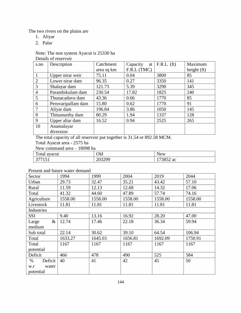
144
The two rivers on the plains are
1. Aliyar
2. Palar
Note: The non system Ayacut is 25330 ha
Details of reservoir
s.no Description Catchment
area sq km
Capacity at
F.R.L (TMC)
F.R.L (ft) Maximum
height (ft)
1 Upper nirar weir 75.11 0.04 3800 85
2 Lower nirar dam 96.35 0.27 3350 141
3 Shalayar dam 121.73 5.39 3290 345
4 Parambikulam dam 230.54 17.82 1825 240
5 Thunacadavu dam 43.36 0.66 1770 85
6 Peruvaripallam dam 15.80 0.62 1770 91
7 Aliyar dam 196.84 3.86 1050 145
8 Thitumurthy dam 80.29 1.94 1337 128
9 Upper aliar dam 16.52 0.94 2525 265
10 Anamalayar
diversion
The total capacity of all reservoir put together is 31.54 or 892.58 MCM.
Total Ayacut area - 2575 ha
New command area – 18098 ha
Total ayacut Old New
377151 203299 173852 ac
Present and future water demand
Sector 1994 1999 2004 2019 2044
Urban 29.73 32.47 35.21 43.42 57.10
Rural 11.59 12.13 12.68 14.32 17.06
Total 41.32 44.60 47.89 57.74 74.16
Agriculture 1558.00 1558.00 1558.00 1558.00 1558.00
Livestock 11.81 11.81 11.81 11.81 11.81
Industries
SSI 9.40 13.16 16.92 28.20 47.00
Large &
medium
12.74 17.46 22.18 36.34 59.94
Sub total 22.14 30.62 39.10 64.54 106.94
Total 1633.27 1645.03 1656.81 1692.09 1750.91
Total
potential
1167 1167 1167 1167 1167
Deficit 466 478 490 525 584
% Deficit
w.r water
potential
40 41 42 45 50

145
Total net irrigation requirement – 1557.62 MCM
Cropping Pattern
s.no Crop Season Duration
in days
1 Paddy
Samba (aug –
sep to dec-jan)
135
Navarai (jan –
mar)
105
Sornavari (apr
-july)
105
2 Groundnut Dec –apr 105
3 Sugarcane Jan - nov 300
4 Cholam - -
5 Cumbu Mar – june 90
6 Ragi - -
7 Vegetables Feb -july 135
8 Pulses Feb - apr 65
9 Gingelly Jan -feb 85
10 Chillies Feb -july 165
Total
The irrigation system of this basin mainly depends on tanks and wells. Canal irrigation is
considerably small. Irrigation sectoral demand is worked out taking into account the conveyance
efficiency, field application efficiency etc. in the present scenario considering all the factor ,the
gross requirement is calculated at 75% overall efficiency for well irrigation and at 40% for canals
and tank irrigation. Net irrigation requirement for various crops and the GIR as worked out are
given below. Irrigation through canals and tanks at 40% efficiency covers 34.26% of gross cropped
area =1415.79 MCM. Irrigation through wells at 75% efficiency covers 65.74 % of gross cropped
area =1448.91 MCM
The overall efficiency of irrigation through canals and tanks have to be stepped out in stages
from 40% to 50% by 2019 AD and from 50% to 60% by 2044 AD corresponding to the above
efficiencies, the irrigation demand were out to2582 MCM at 50% efficiency and 2393 MCM at 60%
efficiency.

146
16. Cauvery basin at grand anicuts
State wise drainage area of Cauvery basin: Karnataka, Kerala, Tamilnadu, Pondicherry.
State Drainage area(Sq Km) % of the total area of the basin
Tamilnadu 43867 54.1
s.no Sub basin State Drainage area
(Sq Km)
% of the total
area
1 Chinnar Tamilnadu 3961 5.79
2 Palar Tamilnadu 1344 4.58
3 Bhavani Tamilnadu 5352 8.78
4 Noyil Tamilnadu 2999 4.28
5 Tirumanimuttar Tamilnadu 8429 12.02
6 Amaravathi Tamilnadu 7896 11.08
7 Ponnanai Tamilnadu 2050 2.92
Total
Ground water Tamilnadu
Estimated potential 5962
Exisisting draft 2869
S.No Name of the sub basin
State /category
1 Chinnar sub basin
a. Thoppaiyar reservoir
b. Chinnar reservoir
c. Kasavigulihall reservoir
d. Nagavathi reservoir
2 Palar sub basin
3 Bhavani sub basin
a. Kodiveri anicuts
b. Lower Bhavani
c. Mettur channel
d. Gunderipallam
e. Varattapallam
4 Noyil sub basin
a. Noyil river channels
b. P.A.P system
c. Lower Bhavani
d. Kalingarayar anicut
5 Tirumanimuttar sub basin
a. Mettur canals

147
b. Lower bhavani
c. Salem Tiruchi channels
d. Katalai canal scheme
e. Kalingarayar anicut
6 Amaravathi sub basin
a. Old Amaravathi channel
b. Amaravathi reservoir
e. P.A.P system
f. Palar- porandalar scheme
g. Varadamanadhi
h. Upper reservoir
i. Parappalar scheme
j. Vattamalai karai odai scheme
7 Ponnanai sub basin
a. Salem – tiruchi channels
b. Katalai canal scheme
c. New Katalai HLC
d. Ponnanai Ar reservoir
s.no Name of the basin Estimated
potential
Exisisting draft Catchment area
1 Upper Cauvery 0 0 10619
2 Kabini 7 0 7040
3 Suvarnavathi 95 55 1787
4 Middle Cauvery 0 0 2676
5 Shimsha 0 0 8469
6 Arkavathi 27 10 4351
7 Chinnar 659 254 4061
8 Palar 230 133 3214
9 Bhavani 617 330 6154
10 Noyil 475 290 2999
11 Thirumanimuthar 1823 926 8429
12 Amaravathi 1489 696 8280
13 Ponnanai Ar 540 175 2050
Total 5962 2869 70129

148
17. Gundar river basin
District: Ramnad, V.O.C, Kamarajar, Pasumpon & Madurai
Dams and reservoir
The river gundar is having 5 tributaries namely giridhamal river, terku river, kanal odai,
utharakosamangai and vembar. Flow measurements are being taken in only one location from
where water is diverted into raghunatha –cauvery channel. There is no major reservoir in the basin
there are about 18 anicuts in the upper half of the basin.
In the gundar basin there are about 18 anicuts in the upper half of the basin. Tanks
irrigating a total of 56730 ha.out of this, the system tanks are 526 irrigating an extent of 2263 ha and
non system tanks (maintained by panchayat union) 123 numbers, irrigating an extent of 2263 ha.
The storage capacity of this tank is approximately 330.59 MCM.
Crop water regulation is adopted by gundar basin NIR (mm)
Paddy (105 days) aug / sep -dec-/jan 704.7
Paddy (133 days) Sep / oct – jan /feb 789.3
Cholam Feb -may 402.72
Ragi Feb -may 427.15
Gingelly Dec -mar 340.70
Cotton Feb -july 698.75
Sunflower Jan -may 380.60
Chillies Sep -feb 499.51
Groundnut Jan -apr 365.57
Assuming that there is no increase in command area due to conversion of wet lands for
other usesand due to modernization of tank schemes,the efficiency is increased from 40 % to 50%
in 2019 & 60 % in 2044 AD , the demand during 2019 & 2044 are below
Demand during 2019 AD – 1556 MCM
Demand during 2044AD – 1421 MCM
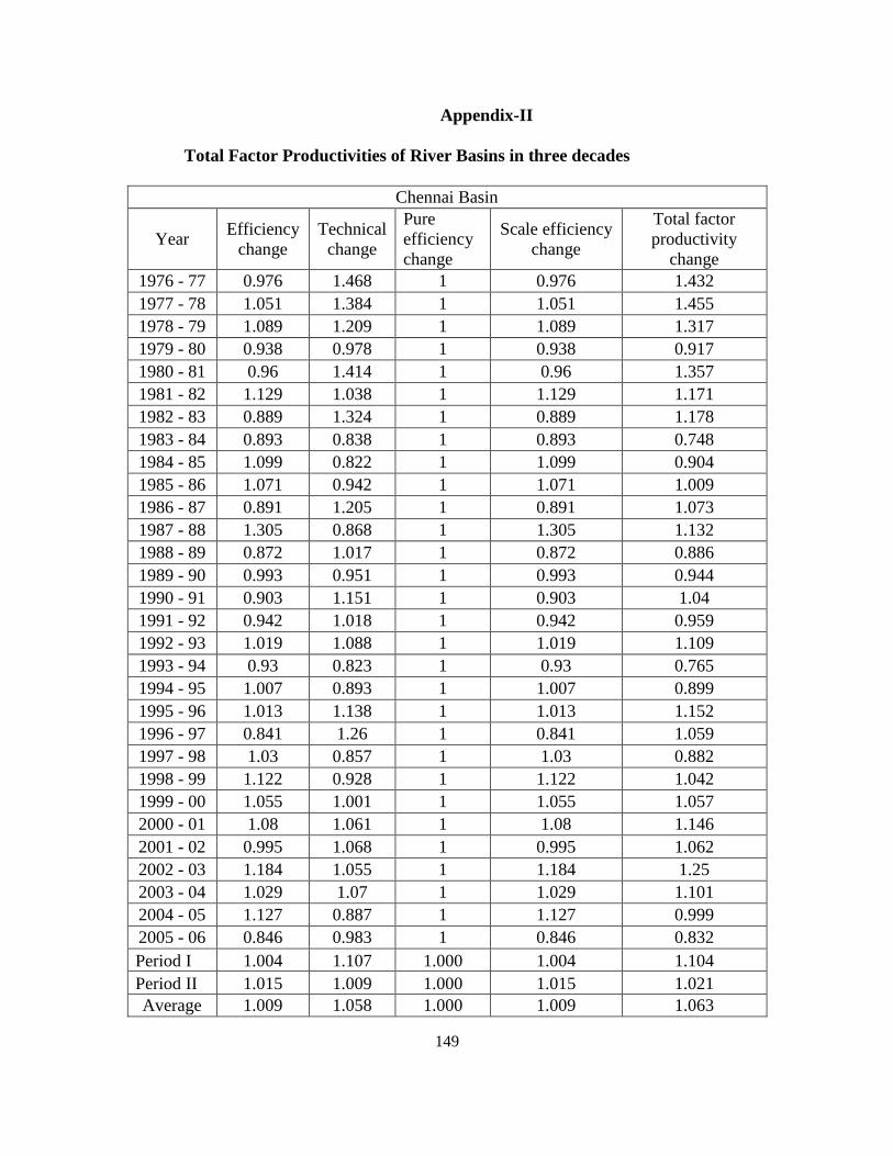
149
Appendix-II
Total Factor Productivities of River Basins in three decades
Chennai Basin
Year Efficiency
change
Technical
change
Pure
efficiency
change
Scale efficiency
change
Total factor
productivity
change
1976 - 77 0.976 1.468 1 0.976 1.432
1977 - 78 1.051 1.384 1 1.051 1.455
1978 - 79 1.089 1.209 1 1.089 1.317
1979 - 80 0.938 0.978 1 0.938 0.917
1980 - 81 0.96 1.414 1 0.96 1.357
1981 - 82 1.129 1.038 1 1.129 1.171
1982 - 83 0.889 1.324 1 0.889 1.178
1983 - 84 0.893 0.838 1 0.893 0.748
1984 - 85 1.099 0.822 1 1.099 0.904
1985 - 86 1.071 0.942 1 1.071 1.009
1986 - 87 0.891 1.205 1 0.891 1.073
1987 - 88 1.305 0.868 1 1.305 1.132
1988 - 89 0.872 1.017 1 0.872 0.886
1989 - 90 0.993 0.951 1 0.993 0.944
1990 - 91 0.903 1.151 1 0.903 1.04
1991 - 92 0.942 1.018 1 0.942 0.959
1992 - 93 1.019 1.088 1 1.019 1.109
1993 - 94 0.93 0.823 1 0.93 0.765
1994 - 95 1.007 0.893 1 1.007 0.899
1995 - 96 1.013 1.138 1 1.013 1.152
1996 - 97 0.841 1.26 1 0.841 1.059
1997 - 98 1.03 0.857 1 1.03 0.882
1998 - 99 1.122 0.928 1 1.122 1.042
1999 - 00 1.055 1.001 1 1.055 1.057
2000 - 01 1.08 1.061 1 1.08 1.146
2001 - 02 0.995 1.068 1 0.995 1.062
2002 - 03 1.184 1.055 1 1.184 1.25
2003 - 04 1.029 1.07 1 1.029 1.101
2004 - 05 1.127 0.887 1 1.127 0.999
2005 - 06 0.846 0.983 1 0.846 0.832
Period I 1.004 1.107 1.000 1.004 1.104
Period II 1.015 1.009 1.000 1.015 1.021
Average 1.009 1.058 1.000 1.009 1.063
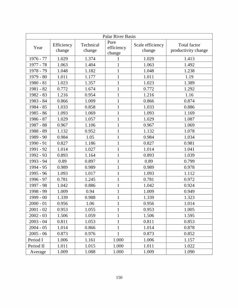
150
Palar River Basin
Year Efficiency
change
Technical
change
Pure
efficiency
change
Scale efficiency
change
Total factor
productivity change
1976 - 77 1.029 1.374 1 1.029 1.413
1977 - 78 1.063 1.404 1 1.063 1.492
1978 - 79 1.048 1.182 1 1.048 1.238
1979 - 80 1.011 1.177 1 1.011 1.19
1980 - 81 1.023 1.357 1 1.023 1.389
1981 - 82 0.772 1.674 1 0.772 1.292
1982 - 83 1.216 0.954 1 1.216 1.16
1983 - 84 0.866 1.009 1 0.866 0.874
1984 - 85 1.033 0.858 1 1.033 0.886
1985 - 86 1.093 1.069 1 1.093 1.169
1986 - 87 1.029 1.057 1 1.029 1.087
1987 - 88 0.967 1.106 1 0.967 1.069
1988 - 89 1.132 0.952 1 1.132 1.078
1989 - 90 0.984 1.05 1 0.984 1.034
1990 - 91 0.827 1.186 1 0.827 0.981
1991 - 92 1.014 1.027 1 1.014 1.041
1992 - 93 0.893 1.164 1 0.893 1.039
1993 - 94 0.89 0.897 1 0.89 0.799
1994 - 95 0.989 0.989 1 0.989 0.978
1995 - 96 1.093 1.017 1 1.093 1.112
1996 - 97 0.781 1.245 1 0.781 0.972
1997 - 98 1.042 0.886 1 1.042 0.924
1998 - 99 1.009 0.94 1 1.009 0.949
1999 - 00 1.339 0.988 1 1.339 1.323
2000 - 01 0.956 1.06 1 0.956 1.014
2001 - 02 0.953 1.055 1 0.953 1.005
2002 - 03 1.506 1.059 1 1.506 1.595
2003 - 04 0.811 1.053 1 0.811 0.853
2004 - 05 1.014 0.866 1 1.014 0.878
2005 - 06 0.873 0.976 1 0.873 0.852
Period I 1.006 1.161 1.000 1.006 1.157
Period II 1.011 1.015 1.000 1.011 1.022
Average 1.009 1.088 1.000 1.009 1.090

151
Varahanadhi River Basin
Year
Efficien
cy
change
Technical
change
Pure efficiency
change Scale efficiency
change
Total factor
productivity change
1976 - 77 1.008 1.503 1 1.008 1.515
1977 - 78 1.004 1.396 1 1.004 1.401
1978 - 79 1.014 1.288 1 1.014 1.306
1979 - 80 0.969 0.931 1 0.969 0.902
1980 - 81 0.987 1.707 1 0.987 1.685
1981 - 82 1.014 1.361 1 1.014 1.381
1982 - 83 0.98 1.044 1 0.98 1.023
1983 - 84 0.98 0.865 1 0.98 0.848
1984 - 85 1.018 0.692 1 1.018 0.705
1985 - 86 1.017 0.992 1 1.017 1.009
1986 - 87 0.984 1.064 1 0.984 1.047
1987 - 88 1.041 1.034 1 1.041 1.076
1988 - 89 0.979 1.138 1 0.979 1.113
1989 - 90 1.022 0.864 1 1.022 0.883
1990 - 91 0.978 1.227 1 0.978 1.2
1991 - 92 0.983 0.986 1 0.983 0.969
1992 - 93 1.001 1.109 1 1.001 1.111
1993 - 94 0.972 0.876 1 0.972 0.852
1994 - 95 1 1.052 1 1 1.052
1995 - 96 1.025 1.009 1 1.025 1.034
1996 - 97 0.959 1.185 1 0.959 1.137
1997 - 98 1.001 0.914 1 1.001 0.915
1998 - 99 1.009 0.945 1 1.009 0.953
1999 - 00 1.047 0.946 1 1.047 0.991
2000 - 01 0.993 1.018 1 0.993 1.011
2001 - 02 0.991 1.039 1 0.991 1.03
2002 - 03 1.061 1.085 1 1.061 1.151
2003 - 04 0.968 1.033 1 0.968 1.001
2004 - 05 1.032 0.958 1 1.032 0.988
2005 - 06 0.986 0.983 1 0.986 0.97
Period I 1.000 1.140 1.000 1.000 1.140
Period II 1.002 1.009 1.000 1.002 1.011
Average 1.001 1.075 1.000 1.001 1.075

152
Ponnaiyar River Basin
Year
Efficien
cy
change
Technical
change
Pure efficiency
change Scale efficiency
change
Total factor
productivity change
1976 - 77 0.99 1.353 1 0.99 1.34
1977 - 78 1.059 1.426 1 1.059 1.509
1978 - 79 1.017 1.176 1 1.017 1.197
1979 - 80 1.829 1.397 1 1.829 2.556
1980 - 81 1.088 1.015 1 1.088 1.105
1981 - 82 1.185 1.467 1 1.185 1.739
1982 - 83 0.885 0.825 1 0.885 0.731
1983 - 84 0.914 1.079 1 0.914 0.986
1984 - 85 0.966 1.016 1 0.966 0.981
1985 - 86 0.969 1.132 1 0.969 1.097
1986 - 87 0.817 0.978 1 0.817 0.799
1987 - 88 0.834 1.439 1 0.834 1.2
1988 - 89 2.193 0.537 1 2.193 1.177
1989 - 90 0.623 1.772 1 0.623 1.104
1990 - 91 0.792 1.149 1 0.792 0.909
1991 - 92 0.775 1.228 1 0.775 0.952
1992 - 93 0.882 0.939 1 0.882 0.828
1993 - 94 0.783 1.109 1 0.783 0.868
1994 - 95 0.914 1.213 1 0.914 1.108
1995 - 96 1.287 0.762 1 1.287 0.982
1996 - 97 0.606 1.327 1 0.606 0.804
1997 - 98 1.024 0.864 1 1.024 0.885
1998 - 99 1.007 0.968 1 1.007 0.975
1999 - 00 1.169 0.939 1 1.169 1.097
2000 - 01 0.985 0.992 1 0.985 0.977
2001 - 02 0.961 1.064 1 0.961 1.022
2002 - 03 1.195 1.011 1 1.195 1.208
2003 - 04 1.088 0.932 1 1.088 1.014
2004 - 05 0.811 0.896 1 0.811 0.727
2005 - 06 0.914 0.996 1 0.914 0.911
Period I 1.077 1.184 1.000 1.077 1.229
Period II 0.960 1.016 1.000 0.960 0.957
Average 1.019 1.100 1.000 1.019 1.093
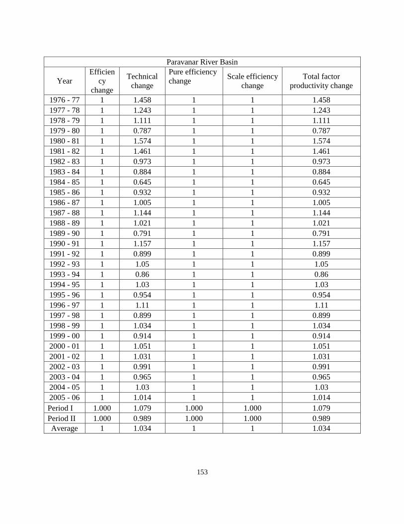
153
Paravanar River Basin
Year
Efficien
cy
change
Technical
change
Pure efficiency
change Scale efficiency
change
Total factor
productivity change
1976 - 77 1 1.458 1 1 1.458
1977 - 78 1 1.243 1 1 1.243
1978 - 79 1 1.111 1 1 1.111
1979 - 80 1 0.787 1 1 0.787
1980 - 81 1 1.574 1 1 1.574
1981 - 82 1 1.461 1 1 1.461
1982 - 83 1 0.973 1 1 0.973
1983 - 84 1 0.884 1 1 0.884
1984 - 85 1 0.645 1 1 0.645
1985 - 86 1 0.932 1 1 0.932
1986 - 87 1 1.005 1 1 1.005
1987 - 88 1 1.144 1 1 1.144
1988 - 89 1 1.021 1 1 1.021
1989 - 90 1 0.791 1 1 0.791
1990 - 91 1 1.157 1 1 1.157
1991 - 92 1 0.899 1 1 0.899
1992 - 93 1 1.05 1 1 1.05
1993 - 94 1 0.86 1 1 0.86
1994 - 95 1 1.03 1 1 1.03
1995 - 96 1 0.954 1 1 0.954
1996 - 97 1 1.11 1 1 1.11
1997 - 98 1 0.899 1 1 0.899
1998 - 99 1 1.034 1 1 1.034
1999 - 00 1 0.914 1 1 0.914
2000 - 01 1 1.051 1 1 1.051
2001 - 02 1 1.031 1 1 1.031
2002 - 03 1 0.991 1 1 0.991
2003 - 04 1 0.965 1 1 0.965
2004 - 05 1 1.03 1 1 1.03
2005 - 06 1 1.014 1 1 1.014
Period I 1.000 1.079 1.000 1.000 1.079
Period II 1.000 0.989 1.000 1.000 0.989
Average 1 1.034 1 1 1.034

154
Vellar Basin
Year
Efficien
cy
change
Technical
change
Pure efficiency
change Scale efficiency
change
Total factor
productivity change
1976 - 77 1.019 1.34 1 1.019 1.366
1977 - 78 0.999 1.389 1 0.999 1.388
1978 - 79 1.006 1.186 1 1.006 1.193
1979 - 80 1.003 1.165 1 1.003 1.169
1980 - 81 1.065 1.338 1 1.065 1.425
1981 - 82 0.865 1.626 1 0.865 1.407
1982 - 83 1.066 0.889 1 1.066 0.948
1983 - 84 0.996 1.01 1 0.996 1.007
1984 - 85 1.114 0.794 1 1.114 0.884
1985 - 86 0.94 1.136 1 0.94 1.068
1986 - 87 0.945 1.063 1 0.945 1.004
1987 - 88 0.933 1.135 1 0.933 1.059
1988 - 89 1.17 0.926 1 1.17 1.083
1989 - 90 0.895 1.14 1 0.895 1.021
1990 - 91 0.897 1.155 1 0.897 1.035
1991 - 92 1.033 1.027 1 1.033 1.061
1992 - 93 0.844 1.231 1 0.844 1.039
1993 - 94 0.88 0.981 1 0.88 0.863
1994 - 95 0.93 1.108 1 0.93 1.031
1995 - 96 1.28 0.886 1 1.28 1.134
1996 - 97 0.762 1.227 1 0.762 0.936
1997 - 98 1.069 0.904 1 1.069 0.966
1998 - 99 1.04 0.931 1 1.04 0.968
1999 - 00 1.107 0.968 1 1.107 1.071
2000 - 01 0.96 1.048 1 0.96 1.006
2001 - 02 0.969 1.01 1 0.969 0.979
2002 - 03 1.217 1.06 1 1.217 1.29
2003 - 04 0.951 1.082 1 0.951 1.03
2004 - 05 0.899 0.937 1 0.899 0.842
2005 - 06 0.834 0.99 1 0.834 0.826
Period I 0.994 1.153 1.000 0.994 1.137
Period II 0.985 1.026 1.000 0.985 1.003
Average 0.990 1.089 1.000 0.990 1.070

155
Cauvery River Basin
Year
Efficien
cy
change
Technical
change
Pure efficiency
change Scale efficiency
change
Total factor
productivity change
1976 - 77 1.001 1.312 1 1.001 1.313
1977 - 78 1 1.368 1 1 1.367
1978 - 79 1.021 1.187 1 1.021 1.213
1979 - 80 1.099 1.126 1 1.099 1.237
1980 - 81 0.895 1.373 1 0.895 1.229
1981 - 82 0.694 1.511 1 0.694 1.048
1982 - 83 1.314 0.849 1 1.314 1.116
1983 - 84 0.924 1.011 1 0.924 0.935
1984 - 85 1.197 0.858 1 1.197 1.027
1985 - 86 0.875 1.141 1 0.875 0.999
1986 - 87 1.002 1.065 1 1.002 1.066
1987 - 88 1.004 0.984 1 1.004 0.988
1988 - 89 1.042 0.993 1 1.042 1.034
1989 - 90 0.915 1.093 1 0.915 0.999
1990 - 91 1.003 1.149 1 1.003 1.153
1991 - 92 0.971 1.042 1 0.971 1.011
1992 - 93 0.919 1.089 1 0.919 1.001
1993 - 94 0.947 0.93 1 0.947 0.881
1994 - 95 0.93 1.023 1 0.93 0.951
1995 - 96 1.191 0.985 1 1.191 1.173
1996 - 97 0.811 1.179 1 0.811 0.957
1997 - 98 1.087 0.903 1 1.087 0.981
1998 - 99 1.079 0.958 1 1.079 1.034
1999 - 00 1.019 0.992 1 1.019 1.011
2000 - 01 0.963 1.031 1 0.963 0.993
2001 - 02 1.077 1.008 1 1.077 1.086
2002 - 03 1.122 1.039 1 1.122 1.165
2003 - 04 1.023 1.026 1 1.023 1.05
2004 - 05 0.921 0.931 1 0.921 0.858
2005 - 06 0.809 1.005 1 0.809 0.813
Period I 0.999 1.135 1.000 0.999 1.115
Period II 0.991 1.009 1.000 0.991 0.998
Average 0.995 1.072 1.000 0.995 1.056
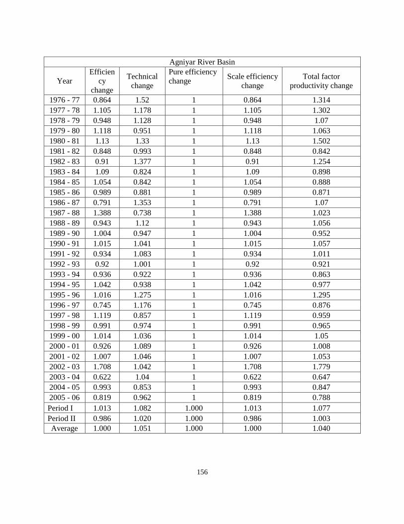
156
Agniyar River Basin
Year
Efficien
cy
change
Technical
change
Pure efficiency
change Scale efficiency
change
Total factor
productivity change
1976 - 77 0.864 1.52 1 0.864 1.314
1977 - 78 1.105 1.178 1 1.105 1.302
1978 - 79 0.948 1.128 1 0.948 1.07
1979 - 80 1.118 0.951 1 1.118 1.063
1980 - 81 1.13 1.33 1 1.13 1.502
1981 - 82 0.848 0.993 1 0.848 0.842
1982 - 83 0.91 1.377 1 0.91 1.254
1983 - 84 1.09 0.824 1 1.09 0.898
1984 - 85 1.054 0.842 1 1.054 0.888
1985 - 86 0.989 0.881 1 0.989 0.871
1986 - 87 0.791 1.353 1 0.791 1.07
1987 - 88 1.388 0.738 1 1.388 1.023
1988 - 89 0.943 1.12 1 0.943 1.056
1989 - 90 1.004 0.947 1 1.004 0.952
1990 - 91 1.015 1.041 1 1.015 1.057
1991 - 92 0.934 1.083 1 0.934 1.011
1992 - 93 0.92 1.001 1 0.92 0.921
1993 - 94 0.936 0.922 1 0.936 0.863
1994 - 95 1.042 0.938 1 1.042 0.977
1995 - 96 1.016 1.275 1 1.016 1.295
1996 - 97 0.745 1.176 1 0.745 0.876
1997 - 98 1.119 0.857 1 1.119 0.959
1998 - 99 0.991 0.974 1 0.991 0.965
1999 - 00 1.014 1.036 1 1.014 1.05
2000 - 01 0.926 1.089 1 0.926 1.008
2001 - 02 1.007 1.046 1 1.007 1.053
2002 - 03 1.708 1.042 1 1.708 1.779
2003 - 04 0.622 1.04 1 0.622 0.647
2004 - 05 0.993 0.853 1 0.993 0.847
2005 - 06 0.819 0.962 1 0.819 0.788
Period I 1.013 1.082 1.000 1.013 1.077
Period II 0.986 1.020 1.000 0.986 1.003
Average 1.000 1.051 1.000 1.000 1.040

157
Pambar & Kottakaraiyar River Basin
Year
Efficien
cy
change
Technical
change
Pure efficiency
change Scale efficiency
change
Total factor
productivity change
1976 - 77 0.991 1.203 1 0.991 1.192
1977 - 78 1.001 1.088 1 1.001 1.09
1978 - 79 0.99 1.023 1 0.99 1.013
1979 - 80 1.146 1.235 1 1.146 1.416
1980 - 81 0.942 1.169 1 0.942 1.101
1981 - 82 0.99 1.153 1 0.99 1.142
1982 - 83 0.927 1.163 1 0.927 1.078
1983 - 84 1.084 0.956 1 1.084 1.036
1984 - 85 1.131 0.972 1 1.131 1.099
1985 - 86 0.997 0.989 1 0.997 0.987
1986 - 87 0.842 1.176 1 0.842 0.991
1987 - 88 1.226 0.867 1 1.226 1.063
1988 - 89 1.01 0.946 1 1.01 0.956
1989 - 90 0.85 1.222 1 0.85 1.038
1990 - 91 0.912 1.065 1 0.912 0.971
1991 - 92 1.106 1.037 1 1.106 1.147
1992 - 93 0.923 1.04 1 0.923 0.961
1993 - 94 0.835 1.07 1 0.835 0.893
1994 - 95 0.995 1.034 1 0.995 1.029
1995 - 96 1.057 0.96 1 1.057 1.015
1996 - 97 0.869 1.076 1 0.869 0.935
1997 - 98 1.052 0.889 1 1.052 0.935
1998 - 99 0.998 0.998 1 0.998 0.995
1999 - 00 1.046 1.034 1 1.046 1.081
2000 - 01 0.98 1.004 1 0.98 0.984
2001 - 02 1.02 1.067 1 1.02 1.088
2002 - 03 1.151 1.034 1 1.151 1.19
2003 - 04 1.082 0.897 1 1.082 0.97
2004 - 05 1.202 0.789 1 1.202 0.949
2005 - 06 0.861 0.968 1 0.861 0.834
Period I 1.003 1.082 1.000 1.003 1.078
Period II 1.012 0.993 1.000 1.012 1.000
Average 1.007 1.037 1.000 1.007 1.039

158
Vaigai River Basin
Year
Efficien
cy
change
Technical
change
Pure efficiency
change Scale efficiency
change
Total factor
productivity change
1976 - 77 1.031 1.09 1 1.031 1.123
1977 - 78 0.995 1.147 1 0.995 1.141
1978 - 79 1.013 1.093 1 1.013 1.107
1979 - 80 1.195 1.082 1 1.195 1.293
1980 - 81 0.733 1.382 1 0.733 1.014
1981 - 82 1.047 1.197 1 1.047 1.254
1982 - 83 1.052 1.03 1 1.052 1.084
1983 - 84 1.004 0.994 1 1.004 0.999
1984 - 85 1.197 0.847 1 1.197 1.014
1985 - 86 0.915 1.133 1 0.915 1.037
1986 - 87 0.908 1.101 1 0.908 1
1987 - 88 0.963 0.911 1 0.963 0.877
1988 - 89 1.011 1.033 1 1.011 1.044
1989 - 90 0.886 1.03 1 0.886 0.913
1990 - 91 0.952 1.107 1 0.952 1.053
1991 - 92 1.064 1.049 1 1.064 1.116
1992 - 93 0.924 1.108 1 0.924 1.024
1993 - 94 0.956 0.962 1 0.956 0.919
1994 - 95 1.029 0.963 1 1.029 0.991
1995 - 96 1.013 1.147 1 1.013 1.162
1996 - 97 0.929 1.017 1 0.929 0.945
1997 - 98 0.998 0.992 1 0.998 0.99
1998 - 99 1.113 1.002 1 1.113 1.115
1999 - 00 0.932 1.008 1 0.932 0.94
2000 - 01 1.038 1.062 1 1.038 1.103
2001 - 02 1.041 1.058 1 1.041 1.101
2002 - 03 1.085 1.04 1 1.085 1.128
2003 - 04 1.072 0.986 1 1.072 1.057
2004 - 05 1.232 0.788 1 1.232 0.971
2005 - 06 0.972 0.94 1 0.972 0.913
Period I 0.993 1.078 1.000 0.993 1.064
Period II 1.027 1.008 1.000 1.027 1.032
Average 1.010 1.043 1.000 1.010 1.048

159
Gundar River Basin
Year
Efficien
cy
change
Technical
change
Pure efficiency
change Scale efficiency
change
Total factor
productivity change
1976 – 77 1.008 1.04 1 1.008 1.048
1977 – 78 1.033 1.188 1 1.033 1.227
1978 – 79 0.936 1.097 1 0.936 1.027
1979 – 80 1.213 1.254 1 1.213 1.521
1980 – 81 0.86 1.107 1 0.86 0.951
1981 – 82 1.135 1.08 1 1.135 1.226
1982 - 83 0.928 1.102 1 0.928 1.022
1983 - 84 1.036 1.045 1 1.036 1.082
1984 - 85 1.128 0.983 1 1.128 1.108
1985 - 86 0.988 1.096 1 0.988 1.083
1986 - 87 0.847 1.179 1 0.847 0.998
1987 - 88 1.04 0.831 1 1.04 0.864
1988 - 89 1.137 0.955 1 1.137 1.086
1989 - 90 0.757 1.119 1 0.757 0.847
1990 - 91 0.885 1.07 1 0.885 0.946
1991 - 92 1.17 0.948 1 1.17 1.11
1992 - 93 0.939 0.967 1 0.939 0.908
1993 - 94 0.903 1.064 1 0.903 0.961
1994 - 95 1.036 0.921 1 1.036 0.954
1995 - 96 1.006 1.056 1 1.006 1.063
1996 - 97 0.937 1.034 1 0.937 0.969
1997 - 98 0.996 0.95 1 0.996 0.947
1998 - 99 1.01 1.002 1 1.01 1.012
1999 - 00 1.027 1.021 1 1.027 1.049
2000 - 01 0.985 1.062 1 0.985 1.046
2001 - 02 1.013 1.125 1 1.013 1.139
2002 - 03 1.06 1.018 1 1.06 1.079
2003 - 04 1.245 0.788 1 1.245 0.981
2004 - 05 1.208 0.77 1 1.208 0.93
2005 - 06 0.923 0.933 1 0.923 0.862
Period I 0.995 1.076 1.000 0.995 1.069
Period II 1.031 0.977 1.000 1.031 1.001
Average 1.013 1.027 1.000 1.013 1.035

160
Vaippar Basin
Year Efficiency
change
Technical
change
Pure efficiency
change Scale efficiency
change
Total factor
productivity
change
1976 - 77 1.011 0.986 1 1.011 0.997
1977 - 78 1.043 1.095 1 1.043 1.142
1978 - 79 0.892 1.013 1 0.892 0.904
1979 - 80 1.352 1.178 1 1.352 1.593
1980 - 81 0.855 1.028 1 0.855 0.879
1981 - 82 1.142 0.991 1 1.142 1.132
1982 - 83 0.872 1.096 1 0.872 0.956
1983 - 84 0.957 0.999 1 0.957 0.955
1984 - 85 1.2 0.962 1 1.2 1.154
1985 - 86 0.968 1.15 1 0.968 1.113
1986 - 87 1.004 1.005 1 1.004 1.009
1987 - 88 0.847 0.915 1 0.847 0.775
1988 - 89 1.113 0.89 1 1.113 0.99
1989 - 90 0.783 1.141 1 0.783 0.894
1990 - 91 0.924 1.007 1 0.924 0.93
1991 - 92 1.287 0.761 1 1.287 0.98
1992 - 93 0.913 0.943 1 0.913 0.862
1993 - 94 0.848 1.052 1 0.848 0.892
1994 - 95 1.122 0.844 1 1.122 0.947
1995 - 96 0.994 0.957 1 0.994 0.952
1996 - 97 0.95 1.042 1 0.95 0.99
1997 - 98 1.006 0.829 1 1.006 0.834
1998 - 99 0.855 1.037 1 0.855 0.886
1999 - 00 1.085 1.016 1 1.085 1.102
2000 - 01 0.959 1.018 1 0.959 0.977
2001 - 02 1.009 1.163 1 1.009 1.173
2002 - 03 0.989 1.049 1 0.989 1.038
2003 - 04 1.101 0.768 1 1.101 0.845
2004 - 05 1.009 0.843 1 1.009 0.851
2005 - 06 1.021 0.938 1 1.021 0.958
Period I 0.998 1.030 1.000 0.998 1.028
Period II 1.010 0.951 1.000 1.010 0.952
Average 1.004 0.991 1.000 1.004 0.990

161
Kallar River Basin
Year
Efficien
cy
change
Technical
change
Pure efficiency
change Scale efficiency
change
Total factor
productivity change
1976 - 77 1 1.09 1 1 1.09
1977 - 78 1 1.057 1 1 1.057
1978 - 79 1 1.045 1 1 1.045
1979 - 80 1 1.258 1 1 1.258
1980 - 81 1 1.052 1 1 1.052
1981 - 82 1 0.998 1 1 0.998
1982 - 83 1 1.14 1 1 1.14
1983 - 84 1 0.961 1 1 0.961
1984 - 85 1 0.677 1 1 0.677
1985 - 86 1 1.027 1 1 1.027
1986 - 87 1 1.608 1 1 1.608
1987 - 88 1 0.811 1 1 0.811
1988 - 89 1 0.776 1 1 0.776
1989 - 90 1 1.257 1 1 1.257
1990 - 91 1 1.006 1 1 1.006
1991 - 92 1 1.011 1 1 1.011
1992 - 93 1 0.961 1 1 0.961
1993 - 94 1 1.136 1 1 1.136
1994 - 95 1 0.991 1 1 0.991
1995 - 96 1 1.296 1 1 1.296
1996 - 97 1 0.967 1 1 0.967
1997 - 98 1 0.817 1 1 0.817
1998 - 99 1 1.065 1 1 1.065
1999 - 00 1 1.059 1 1 1.059
2000 - 01 1 1.304 1 1 1.304
2001 - 02 1 1.183 1 1 1.183
2002 - 03 1 0.839 1 1 0.839
2003 - 04 1 0.774 1 1 0.774
2004 - 05 1 0.891 1 1 0.891
2005 - 06 1 0.915 1 1 0.915
Period I 1.000 1.051 1.000 1.000 1.051
Period II 1.000 1.014 1.000 1.000 1.014
Average 1 1.032 1 1 1.032
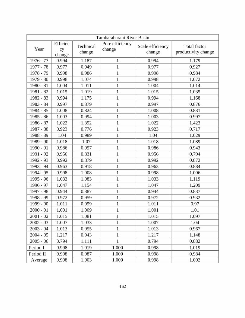
162
Tambarabarani River Basin
Year
Efficien
cy
change
Technical
change
Pure efficiency
change Scale efficiency
change
Total factor
productivity change
1976 - 77 0.994 1.187 1 0.994 1.179
1977 - 78 0.977 0.949 1 0.977 0.927
1978 - 79 0.998 0.986 1 0.998 0.984
1979 - 80 0.998 1.074 1 0.998 1.072
1980 - 81 1.004 1.011 1 1.004 1.014
1981 - 82 1.015 1.019 1 1.015 1.035
1982 - 83 0.994 1.175 1 0.994 1.168
1983 - 84 0.997 0.879 1 0.997 0.876
1984 - 85 1.008 0.824 1 1.008 0.831
1985 - 86 1.003 0.994 1 1.003 0.997
1986 - 87 1.022 1.392 1 1.022 1.423
1987 - 88 0.923 0.776 1 0.923 0.717
1988 - 89 1.04 0.989 1 1.04 1.029
1989 - 90 1.018 1.07 1 1.018 1.089
1990 - 91 0.986 0.957 1 0.986 0.943
1991 - 92 0.956 0.831 1 0.956 0.794
1992 - 93 0.992 0.879 1 0.992 0.872
1993 - 94 0.963 0.918 1 0.963 0.884
1994 - 95 0.998 1.008 1 0.998 1.006
1995 - 96 1.033 1.083 1 1.033 1.119
1996 - 97 1.047 1.154 1 1.047 1.209
1997 - 98 0.944 0.887 1 0.944 0.837
1998 - 99 0.972 0.959 1 0.972 0.932
1999 - 00 1.011 0.959 1 1.011 0.97
2000 - 01 1.001 1.009 1 1.001 1.01
2001 - 02 1.015 1.081 1 1.015 1.097
2002 - 03 1.007 1.033 1 1.007 1.04
2003 - 04 1.013 0.955 1 1.013 0.967
2004 - 05 1.217 0.943 1 1.217 1.148
2005 - 06 0.794 1.111 1 0.794 0.882
Period I 0.998 1.019 1.000 0.998 1.019
Period II 0.998 0.987 1.000 0.998 0.984
Average 0.998 1.003 1.000 0.998 1.002

163
Nambiyar River Basin
Year
Efficien
cy
change
Technical
change
Pure efficiency
change Scale efficiency
change
Total factor
productivity change
1976 - 77 1 1.152 1 1 1.152
1977 - 78 1 0.963 1 1 0.963
1978 - 79 1 0.963 1 1 0.963
1979 - 80 1 1.145 1 1 1.145
1980 - 81 1 1.032 1 1 1.032
1981 - 82 1 0.949 1 1 0.949
1982 - 83 1 1.154 1 1 1.154
1983 - 84 1 0.896 1 1 0.896
1984 - 85 1 0.739 1 1 0.739
1985 - 86 1 0.942 1 1 0.942
1986 - 87 1 1.416 1 1 1.416
1987 - 88 1 0.725 1 1 0.725
1988 - 89 1 0.975 1 1 0.975
1989 - 90 1 1.046 1 1 1.046
1990 - 91 1 0.963 1 1 0.963
1991 - 92 1 0.839 1 1 0.839
1992 - 93 1 0.921 1 1 0.921
1993 - 94 1 0.935 1 1 0.935
1994 - 95 1 0.956 1 1 0.956
1995 - 96 1 1.084 1 1 1.084
1996 - 97 1 1.119 1 1 1.119
1997 - 98 1 0.853 1 1 0.853
1998 - 99 1 0.937 1 1 0.937
1999 - 00 1 0.948 1 1 0.948
2000 - 01 1 0.984 1 1 0.984
2001 - 02 1 1.081 1 1 1.081
2002 - 03 1 1.048 1 1 1.048
2003 - 04 1 0.889 1 1 0.889
2004 - 05 1 0.927 1 1 0.927
2005 - 06 1 1.502 1 1 1.502
Period I 1.000 1.004 1.000 1.000 1.004
Period II 1.000 1.002 1.000 1.000 1.002
Average 1 1.003 1 1 1.003

164
Kodaiyar River Basin
Year
Efficien
cy
change
Technical
change
Pure efficiency
change Scale efficiency
change
Total factor
productivity change
1976 - 77 1.006 2.082 1 1.006 2.094
1977 - 78 1 0.71 1 1 0.71
1978 - 79 1 1.162 1 1 1.162
1979 - 80 1 0.993 1 1 0.993
1980 - 81 1 1.042 1 1 1.042
1981 - 82 1 0.818 1 1 0.818
1982 - 83 1 1.076 1 1 1.076
1983 - 84 1 0.986 1 1 0.986
1984 - 85 1 0.677 1 1 0.677
1985 - 86 1 0.86 1 1 0.86
1986 - 87 1 1.411 1 1 1.411
1987 - 88 1 0.62 1 1 0.62
1988 - 89 1 0.808 1 1 0.808
1989 - 90 1 1.474 1 1 1.474
1990 - 91 1 0.722 1 1 0.722
1991 - 92 1 1.072 1 1 1.072
1992 - 93 1 1.253 1 1 1.253
1993 - 94 1 0.855 1 1 0.855
1994 - 95 1 0.73 1 1 0.73
1995 - 96 1 1.435 1 1 1.435
1996 - 97 1 0.944 1 1 0.944
1997 - 98 1 0.907 1 1 0.907
1998 - 99 1 0.962 1 1 0.962
1999 - 00 1 1.006 1 1 1.006
2000 - 01 1 1.062 1 1 1.062
2001 - 02 1 1.109 1 1 1.109
2002 - 03 1 1.088 1 1 1.088
2003 - 04 1 1.072 1 1 1.072
2004 - 05 1 0.926 1 1 0.926
2005 - 06 1 0.857 1 1 0.857
Period I 1.000 1.029 1.000 1.000 1.030
Period II 1.000 1.019 1.000 1.000 1.019
Average 1.000 1.024 1.000 1.000 1.024

165
P.A.P. Basin
Year
Efficie
ncy
chang
e
Technical
change
Pure efficiency
change Scale efficiency
change
Total factor
productivity change
1976 - 77 1.081 0.9 1 1.081 0.973
1977 - 78 0.899 0.996 1 0.899 0.896
1978 - 79 0.991 0.975 1 0.991 0.967
1979 - 80 0.994 0.991 1 0.994 0.985
1980 - 81 0.992 0.997 1 0.992 0.989
1981 - 82 0.986 0.997 1 0.986 0.983
1982 - 83 1 0.993 1 1 0.993
1983 - 84 0.998 0.984 1 0.998 0.982
1984 - 85 0.994 0.797 1 0.994 0.792
1985 - 86 0.998 0.993 1 0.998 0.992
1986 - 87 0.977 1.011 1 0.977 0.987
1987 - 88 1.011 0.981 1 1.011 0.992
1988 - 89 1.012 0.983 1 1.012 0.995
1989 - 90 0.993 0.995 1 0.993 0.988
1990 - 91 1.083 0.967 1 1.083 1.048
1991 - 92 0.903 1.026 1 0.903 0.926
1992 - 93 0.981 0.995 1 0.981 0.976
1993 - 94 1.002 0.997 1 1.002 0.999
1994 - 95 1.007 1.001 1 1.007 1.008
1995 - 96 0.983 0.992 1 0.983 0.975
1996 - 97 0.992 1.01 1 0.992 1.003
1997 - 98 1.011 0.984 1 1.011 0.994
1998 - 99 1.003 0.997 1 1.003 1
1999 - 00 0.992 0.988 1 0.992 0.98
2000 - 01 0.961 1.033 1 0.961 0.993
2001 - 02 0.992 1.083 1 0.992 1.074
2002 - 03 1.019 1 1 1.019 1.018
2003 - 04 1.027 0.891 1 1.027 0.915
2004 - 05 1.14 0.772 1 1.14 0.88
2005 - 06 1.054 0.931 1 1.054 0.981
Period I 1.001 0.971 1.000 1.001 0.971
Period II 1.004 0.980 1.000 1.004 0.981
Average 1.003 0.975 1.000 1.003 0.976

166
Appendix-III Summary of TFP Indices
a) Small basins
Year Chennai Varaha Paravan Agniyar Kallar Tambara Nambiyar Kodaiyar PAP
1976 1.432 1.515 1.458 1.314 1.09 1.179 1.152 2.094 0.973
1977 1.455 1.401 1.243 1.302 1.057 0.927 0.963 0.71 0.896
1978 1.317 1.306 1.111 1.07 1.045 0.984 0.963 1.162 0.967
1979 0.917 0.902 0.787 1.063 1.258 1.072 1.145 0.993 0.985
1980 1.357 1.685 1.574 1.502 1.052 1.014 1.032 1.042 0.989
1981 1.171 1.381 1.461 0.842 0.998 1.035 0.949 0.818 0.983
1982 1.178 1.023 0.973 1.254 1.14 1.168 1.154 1.076 0.993
1983 0.748 0.848 0.884 0.898 0.961 0.876 0.896 0.986 0.982
1984 0.904 0.705 0.645 0.888 0.677 0.831 0.739 0.677 0.792
1985 1.009 1.009 0.932 0.871 1.027 0.997 0.942 0.86 0.992
1986 1.073 1.047 1.005 1.07 1.608 1.423 1.416 1.411 0.987
1987 1.132 1.076 1.144 1.023 0.811 0.717 0.725 0.62 0.992
1988 0.886 1.113 1.021 1.056 0.776 1.029 0.975 0.808 0.995
1989 0.944 0.883 0.791 0.952 1.257 1.089 1.046 1.474 0.988
1990 1.04 1.2 1.157 1.057 1.006 0.943 0.963 0.722 1.048
1991 0.959 0.969 0.899 1.011 1.011 0.794 0.839 1.072 0.926
1992 1.109 1.111 1.05 0.921 0.961 0.872 0.921 1.253 0.976
1993 0.765 0.852 0.86 0.863 1.136 0.884 0.935 0.855 0.999
1994 0.899 1.052 1.03 0.977 0.991 1.006 0.956 0.73 1.008
1995 1.152 1.034 0.954 1.295 1.296 1.119 1.084 1.435 0.975
1996 1.059 1.137 1.11 0.876 0.967 1.209 1.119 0.944 1.003
1997 0.882 0.915 0.899 0.959 0.817 0.837 0.853 0.907 0.994
1998 1.042 0.953 1.034 0.965 1.065 0.932 0.937 0.962 1
1999 1.057 0.991 0.914 1.05 1.059 0.97 0.948 1.006 0.98
2000 1.146 1.011 1.051 1.008 1.304 1.01 0.984 1.062 0.993
2001 1.062 1.03 1.031 1.053 1.183 1.097 1.081 1.109 1.074
2002 1.25 1.151 0.991 1.779 0.839 1.04 1.048 1.088 1.018
2003 1.101 1.001 0.965 0.647 0.774 0.967 0.889 1.072 0.915
2004 0.999 0.988 1.03 0.847 0.891 1.148 0.927 0.926 0.88
2005 0.832 0.97 1.014 0.788 0.915 0.882 1.502 0.857 0.981

167
b) Medium Basins
Year Vellar Pambar Vaigai Gundar Vaippar
1976 1.366 1.192 1.123 1.048 0.997
1977 1.388 1.09 1.141 1.227 1.142
1978 1.193 1.013 1.107 1.027 0.904
1979 1.169 1.416 1.293 1.521 1.593
1980 1.425 1.101 1.014 0.951 0.879
1981 1.407 1.142 1.254 1.226 1.132
1982 0.948 1.078 1.084 1.022 0.956
1983 1.007 1.036 0.999 1.082 0.955
1984 0.884 1.099 1.014 1.108 1.154
1985 1.068 0.987 1.037 1.083 1.113
1986 1.004 0.991 1 0.998 1.009
1987 1.059 1.063 0.877 0.864 0.775
1988 1.083 0.956 1.044 1.086 0.99
1989 1.021 1.038 0.913 0.847 0.894
1990 1.035 0.971 1.053 0.946 0.93
1991 1.061 1.147 1.116 1.11 0.98
1992 1.039 0.961 1.024 0.908 0.862
1993 0.863 0.893 0.919 0.961 0.892
1994 1.031 1.029 0.991 0.954 0.947
1995 1.134 1.015 1.162 1.063 0.952
1996 0.936 0.935 0.945 0.969 0.99
1997 0.966 0.935 0.99 0.947 0.834
1998 0.968 0.995 1.115 1.012 0.886
1999 1.071 1.081 0.94 1.049 1.102
2000 1.006 0.984 1.103 1.046 0.977
2001 0.979 1.088 1.101 1.139 1.173
2002 1.29 1.19 1.128 1.079 1.038
2003 1.03 0.97 1.057 0.981 0.845
2004 0.842 0.949 0.971 0.93 0.851
2005 0.826 0.834 0.913 0.862 0.958

168
c) Large Basins
Year Palar Ponnaiya Cauvery
1976 1.413 1.34 1.313
1977 1.492 1.509 1.367
1978 1.238 1.197 1.213
1979 1.19 2.556 1.237
1980 1.389 1.105 1.229
1981 1.292 1.739 1.048
1982 1.16 0.731 1.116
1983 0.874 0.986 0.935
1984 0.886 0.981 1.027
1985 1.169 1.097 0.999
1986 1.087 0.799 1.066
1987 1.069 1.2 0.988
1988 1.078 1.177 1.034
1989 1.034 1.104 0.999
1990 0.981 0.909 1.153
1991 1.041 0.952 1.011
1992 1.039 0.828 1.001
1993 0.799 0.868 0.881
1994 0.978 1.108 0.951
1995 1.112 0.982 1.173
1996 0.972 0.804 0.957
1997 0.924 0.885 0.981
1998 0.949 0.975 1.034
1999 1.323 1.097 1.011
2000 1.014 0.977 0.993
2001 1.005 1.022 1.086
2002 1.595 1.208 1.165
2003 0.853 1.014 1.05
2004 0.878 0.727 0.858
2005 0.852 0.911 0.813
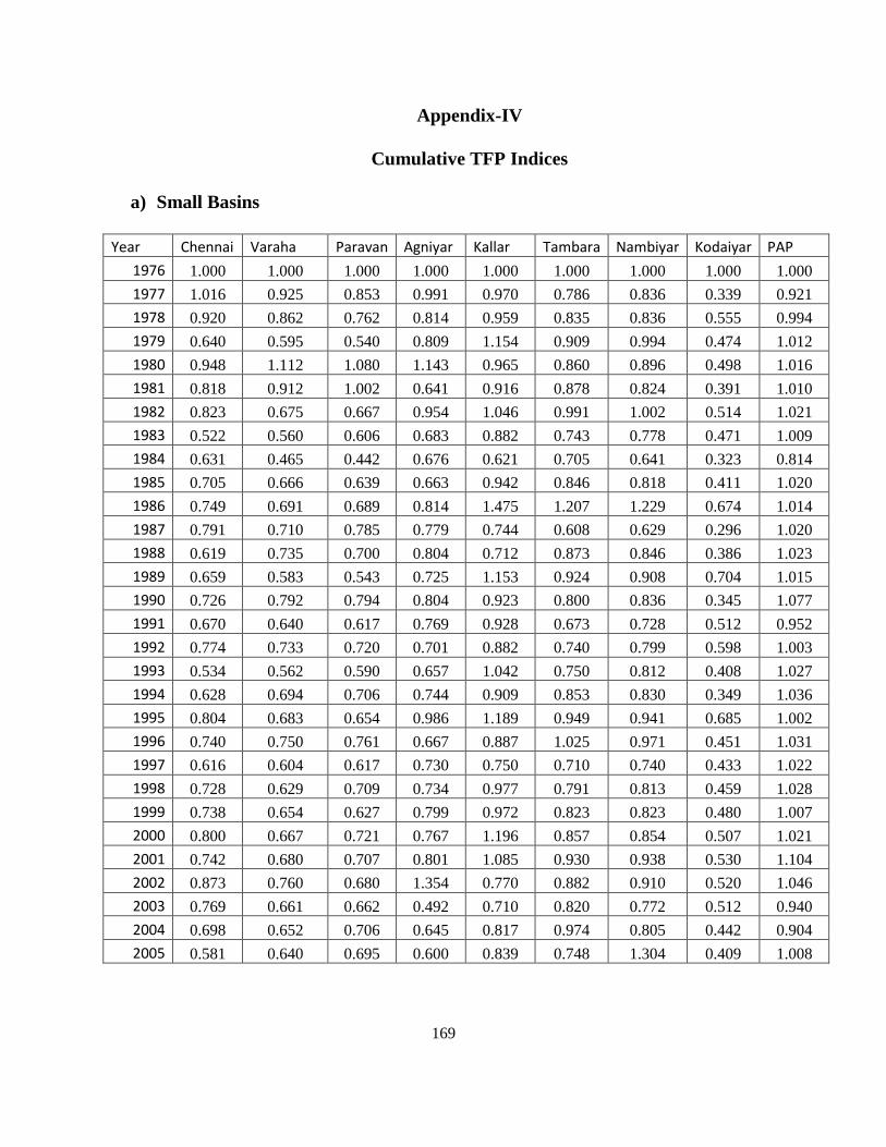
169
Appendix-IV
Cumulative TFP Indices
a) Small Basins
Year Chennai Varaha Paravan Agniyar Kallar Tambara Nambiyar Kodaiyar PAP
1976 1.000 1.000 1.000 1.000 1.000 1.000 1.000 1.000 1.000
1977 1.016 0.925 0.853 0.991 0.970 0.786 0.836 0.339 0.921
1978 0.920 0.862 0.762 0.814 0.959 0.835 0.836 0.555 0.994
1979 0.640 0.595 0.540 0.809 1.154 0.909 0.994 0.474 1.012
1980 0.948 1.112 1.080 1.143 0.965 0.860 0.896 0.498 1.016
1981 0.818 0.912 1.002 0.641 0.916 0.878 0.824 0.391 1.010
1982 0.823 0.675 0.667 0.954 1.046 0.991 1.002 0.514 1.021
1983 0.522 0.560 0.606 0.683 0.882 0.743 0.778 0.471 1.009
1984 0.631 0.465 0.442 0.676 0.621 0.705 0.641 0.323 0.814
1985 0.705 0.666 0.639 0.663 0.942 0.846 0.818 0.411 1.020
1986 0.749 0.691 0.689 0.814 1.475 1.207 1.229 0.674 1.014
1987 0.791 0.710 0.785 0.779 0.744 0.608 0.629 0.296 1.020
1988 0.619 0.735 0.700 0.804 0.712 0.873 0.846 0.386 1.023
1989 0.659 0.583 0.543 0.725 1.153 0.924 0.908 0.704 1.015
1990 0.726 0.792 0.794 0.804 0.923 0.800 0.836 0.345 1.077
1991 0.670 0.640 0.617 0.769 0.928 0.673 0.728 0.512 0.952
1992 0.774 0.733 0.720 0.701 0.882 0.740 0.799 0.598 1.003
1993 0.534 0.562 0.590 0.657 1.042 0.750 0.812 0.408 1.027
1994 0.628 0.694 0.706 0.744 0.909 0.853 0.830 0.349 1.036
1995 0.804 0.683 0.654 0.986 1.189 0.949 0.941 0.685 1.002
1996 0.740 0.750 0.761 0.667 0.887 1.025 0.971 0.451 1.031
1997 0.616 0.604 0.617 0.730 0.750 0.710 0.740 0.433 1.022
1998 0.728 0.629 0.709 0.734 0.977 0.791 0.813 0.459 1.028
1999 0.738 0.654 0.627 0.799 0.972 0.823 0.823 0.480 1.007
2000 0.800 0.667 0.721 0.767 1.196 0.857 0.854 0.507 1.021
2001 0.742 0.680 0.707 0.801 1.085 0.930 0.938 0.530 1.104
2002 0.873 0.760 0.680 1.354 0.770 0.882 0.910 0.520 1.046
2003 0.769 0.661 0.662 0.492 0.710 0.820 0.772 0.512 0.940
2004 0.698 0.652 0.706 0.645 0.817 0.974 0.805 0.442 0.904
2005 0.581 0.640 0.695 0.600 0.839 0.748 1.304 0.409 1.008

170
b) Medium Basins
Year Vellar Pambar Vaigai Gundar Vaippar
1976 1.000 1.000 1.000 1.000 1.000
1977 1.016 0.914 1.016 1.171 1.145
1978 0.873 0.850 0.986 0.980 0.907
1979 0.856 1.188 1.151 1.451 1.598
1980 1.043 0.924 0.903 0.907 0.882
1981 1.030 0.958 1.117 1.170 1.135
1982 0.694 0.904 0.965 0.975 0.959
1983 0.737 0.869 0.890 1.032 0.958
1984 0.647 0.922 0.903 1.057 1.157
1985 0.782 0.828 0.923 1.033 1.116
1986 0.735 0.831 0.890 0.952 1.012
1987 0.775 0.892 0.781 0.824 0.777
1988 0.793 0.802 0.930 1.036 0.993
1989 0.747 0.871 0.813 0.808 0.897
1990 0.758 0.815 0.938 0.903 0.933
1991 0.777 0.962 0.994 1.059 0.983
1992 0.761 0.806 0.912 0.866 0.865
1993 0.632 0.749 0.818 0.917 0.895
1994 0.755 0.863 0.882 0.910 0.950
1995 0.830 0.852 1.035 1.014 0.955
1996 0.685 0.784 0.841 0.925 0.993
1997 0.707 0.784 0.882 0.904 0.837
1998 0.709 0.835 0.993 0.966 0.889
1999 0.784 0.907 0.837 1.001 1.105
2000 0.736 0.826 0.982 0.998 0.980
2001 0.717 0.913 0.980 1.087 1.177
2002 0.944 0.998 1.004 1.030 1.041
2003 0.754 0.814 0.941 0.936 0.848
2004 0.616 0.796 0.865 0.887 0.854
2005 0.605 0.700 0.813 0.823 0.961
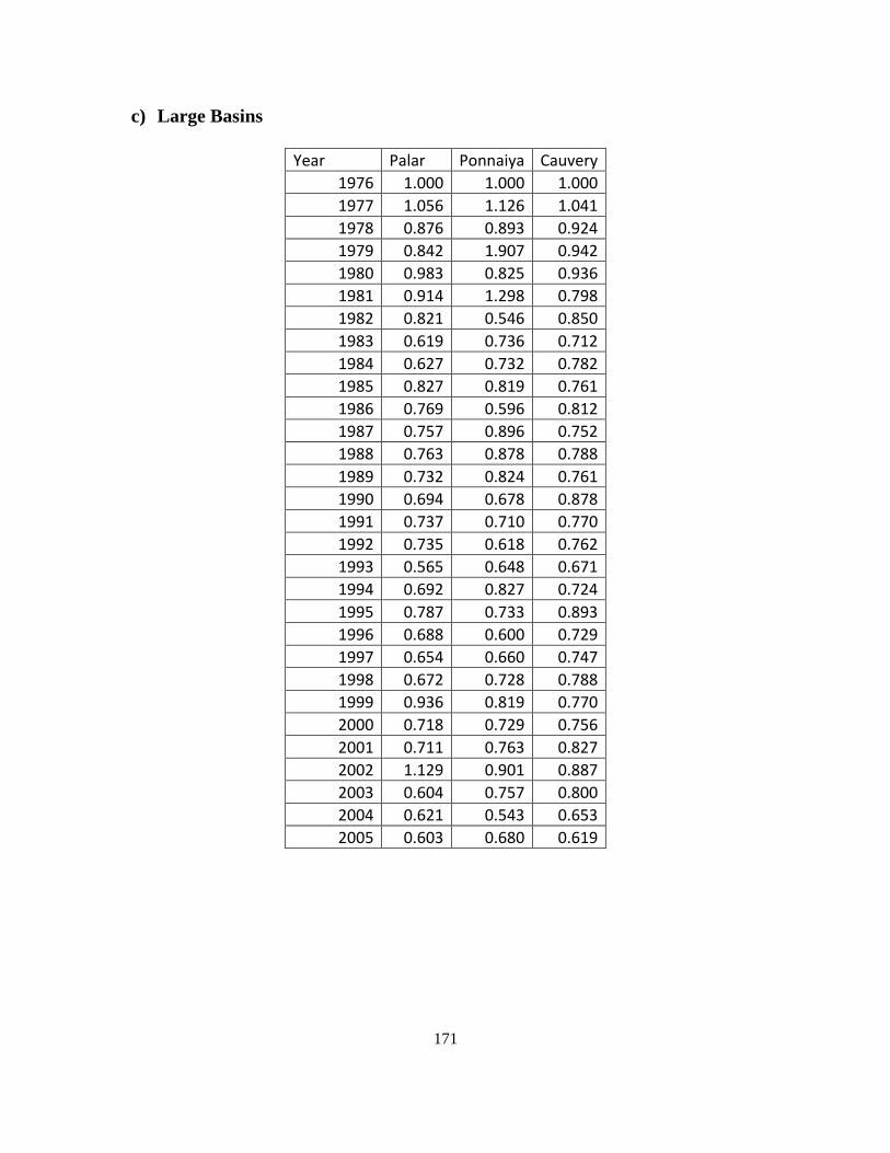
171
c) Large Basins
Year Palar Ponnaiya Cauvery
1976 1.000 1.000 1.000
1977 1.056 1.126 1.041
1978 0.876 0.893 0.924
1979 0.842 1.907 0.942
1980 0.983 0.825 0.936
1981 0.914 1.298 0.798
1982 0.821 0.546 0.850
1983 0.619 0.736 0.712
1984 0.627 0.732 0.782
1985 0.827 0.819 0.761
1986 0.769 0.596 0.812
1987 0.757 0.896 0.752
1988 0.763 0.878 0.788
1989 0.732 0.824 0.761
1990 0.694 0.678 0.878
1991 0.737 0.710 0.770
1992 0.735 0.618 0.762
1993 0.565 0.648 0.671
1994 0.692 0.827 0.724
1995 0.787 0.733 0.893
1996 0.688 0.600 0.729
1997 0.654 0.660 0.747
1998 0.672 0.728 0.788
1999 0.936 0.819 0.770
2000 0.718 0.729 0.756
2001 0.711 0.763 0.827
2002 1.129 0.901 0.887
2003 0.604 0.757 0.800
2004 0.621 0.543 0.653
2005 0.603 0.680 0.619