performance of markov chain–monte carlo approaches for mapping genes in oligogenic models with an...
TRANSCRIPT
Am. J. Hum. Genet. 67:1232–1250, 2000
1232
Performance of Markov Chain–Monte Carlo Approaches for MappingGenes in Oligogenic Models with an Unknown Number of LociJae K. Lee1 and Duncan C. Thomas2
1Department of Health Evaluation Sciences, University of Virginia School of Medicine, Charlottesville, and 2Department of PreventiveMedicine, University of Southern California, Los Angeles
Markov chain–Monte Carlo (MCMC) techniques for multipoint mapping of quantitative trait loci have beendeveloped on nuclear-family and extended-pedigree data. These methods are based on repeated sampling—peelingand gene dropping of genotype vectors and random sampling of each of the model parameters from their fullconditional distributions, given phenotypes, markers, and other model parameters. We further refine such approachesby improving the efficiency of the marker haplotype-updating algorithm and by adopting a new proposal for addingloci. Incorporating these refinements, we have performed an extensive simulation study on simulated nuclear-familydata, varying the number of trait loci, family size, displacement, and other segregation parameters. Our simulationstudies show that our MCMC algorithm identifies the locations of the true trait loci and estimates their segregationparameters well—provided that the total number of sibship pairs in the pedigree data is reasonably large, heritabilityof each individual trait locus is not too low, and the loci are not too close together. Our MCMC algorithm wasshown to be significantly more efficient than LOKI (Heath 1997) in our simulation study using nuclear-family data.
Introduction
Quantitative trait-locus (QTL) mapping methods havebeen well established in experimental genetics (see, e.g.,Lander and Botstein 1989; Kruglyak and Lander 1995).Recently, there has been a surge of interest in Bayesianapproaches to mapping QTLs. Although the origins ofthese methods are in the plant- and animal-breedingfields (Jansen and Stam 1994; Jansen 1996) and arebased on experimental crosses between highly inbredlines, similar approaches have recently been explored inhuman genetics. In experimental genetics, the samplesin the offspring generation are treated as independentobservations using a relatively simple regression of thephenotype on a putative genotype, whose probabilitydistribution is related to the observed marker data. Ste-phens and Smith (1993), Satagopan et al. (1996), andUimari et al. (1996) describe Markov chain–MonteCarlo (MCMC) implementations of a fully Bayesiantreatment of the problem of estimating both the locationand segregation parameters for multiple QTLs, wherethe number of QTLs is fixed. However, the number ofQTLs is in fact unknown, and hence the dimensionality
Received May 15, 2000; accepted for publication August 21, 2000;electronically published October 13, 2000.
Address for correspondence and reprints: Dr. Jae K. Lee, Departmentof Health Evaluation Sciences, University of Virginia School of Med-icine, P.O. Box 800717, Charlottesville, VA 22908. E-mail: [email protected]
� 2000 by The American Society of Human Genetics. All rights reserved.0002-9297/2000/6705-0021$02.00
of the parameter space is also unknown, a problem thathas not been solvable in a Bayesian framework until theintroduction of the reversible-jump MCMC method byGreen (1995). Sillanpaa and Arjas (1998, 1999) andStevens and Fisch (1998) applied this approach to thecase of an unknown number of QTLs in line crosses,and George et al. (2000) applied similar methods to theproblem of ordering marker loci. Although these meth-ods, and the related methods in human genetics, wereoriginally developed for mapping genes involved inquantitative traits, they are easily extended to binary,censored age at onset, or multivariate traits; nevertheless,we retain the term “QTL” in this discussion because ofits historical context, without wishing to imply any suchrestriction.
The application of these ideas to human genetics isrelatively new. Additional complications in human ge-netics derive from the absence of simple experimental-cross designs, leading to the need to consider all possiblehaplotypes corresponding to the observed genotypes,missing marker data on some individuals, more-com-plex pedigree structures, and uncertainty about the formof the disease model. At the 10th Genetic AnalysisWorkshop (GAW), Heath et al. (1997) and Thomas etal. (1997) independently introduced similar methodsbased on reversible-jump MCMC, where the genotypesat the trait loci were sampled using peeling, conditionalon the current assignments of locations and segregationparameters. Given these sampled genotypes, the updat-ing of these parameters and the number of trait locithen followed methods similar to those used in breed-
Lee and Thomas: MCMC Approaches for Mapping Genes in Oligogenic Mode 1233
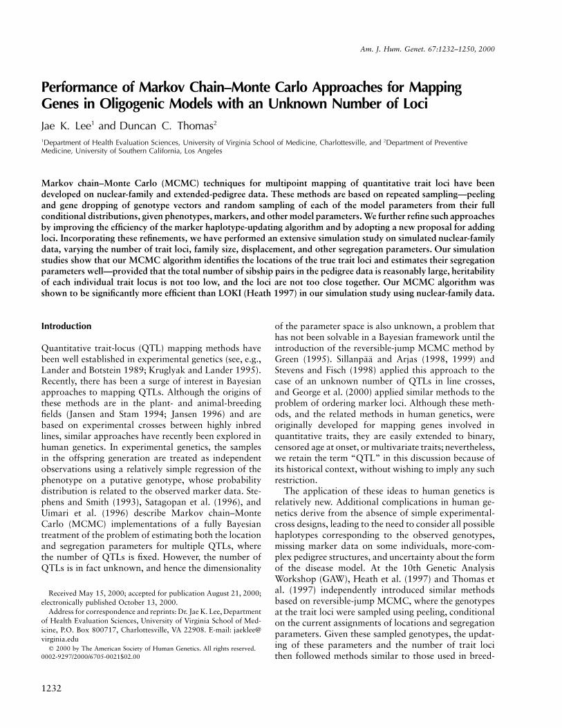
Figure 1 Directed acyclic graph for the QTL mapping model.Squares indicate observed data (X, H, and Y) or fixed hyperparametersl. Circles indicate unknown parameters ( ) or latent var-G , S , and T� �
iables ( ). Not shown are the hyperpriors f forx , q , b , d , and G q� � � � �
and q for .b�
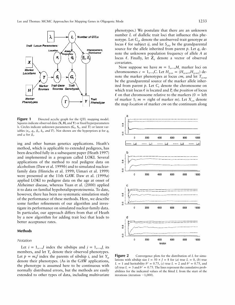
Figure 2 Convergence plots for the distribution of L for simu-lations with sibship size for (a) true , (b) trueI p 50 # J p 8 L p 0
and heritability , (c) true and , and2 2L p 1 h p 0.75 L p 2 h p 0.75(d) true and . The lines represent the cumulative prob-2L p 3 h p 0.75abilities for the indicated values of the fitted L from the start of theiterations (iteration �1,000).
ing and other human genetics applications. Heath’smethod, which is applicable to extended pedigrees, hasbeen described fully in a subsequent paper (Heath 1997)and implemented in a program called LOKI. Severalapplications of the method to real pedigree data onalcoholism (Daw et al. 1999b) and to simulated nuclear-family data (Hinrichs et al. 1999; Uimari et al. 1999)were presented at the 11th GAW. Daw et al. (1999a)applied LOKI to pedigree data on the age at onset ofAlzheimer disease, whereas Yuan et al. (2000) appliedit to data on familial hypobetalipoproteinemia. To date,however, there has been no systematic simulation studyof the performance of these methods. Here, we describesome further refinements of our algorithm and inves-tigate its performance on simulated nuclear-family data.In particular, our approach differs from that of Heathby a new algorithm for adding trait loci that leads tobetter acceptance rates.
Methods
Notation
Let index the sibships and itsi p 1,...,I j p 1,...,Ji
members, and let denote their observed phenotypes.Yij
Let index the parents of sibship i, and letp p m,f Yip
denote their phenotypes. (As in the GAW applications,the phenotype is assumed here to be continuous withnormally distributed errors, but the methods are easilyextended to other types of data, including multivariate
phenotypes.) We postulate that there are an unknownnumber L of diallelic trait loci that influence this phe-notype. Let denote the unobserved trait genotype atGij�
locus for subject ij, and let be the grandparental� Sij�p
source for the allele inherited from parent p. Let de-q�
note the unknown population frequency of allele A atlocus . Finally, let denote a vector of observed� Zij
covariates.Now suppose we have marker loci onm p 1,...,Mc
chromosomes . Let de-c p 1,...,C H p (H ,H )ijcm ijcm1 ijcm2
note the marker phenotypes at locus cm, and let Tijcmp
be the grandparental source of the marker allele inher-ited from parent p. Let denote the chromosome onC�
which trait locus is located and the position of locus� P�
on that chromosome relative to the markers (0 p left�of marker 1; m p right of marker m). Let denoteXcm
the map location of marker cm on the continuum along
1234 Am. J. Hum. Genet. 67:1232–1250, 2000
Table 1
BFs for the Number of Trait Loci when True L Varies from 0 to 5
MODEL I#JHERITABILITY
(h2)
BFS FOR FITTED L
0 1 2 3 4 5�
0 50#8 0 6.60 3.35 .67 .08 .00 .001a 50#8 .10 5.92 3.44 .74 .10 .01 .001b 50#8 .25 .12 3.10 1.79 .50 .09 .001c 50#8 .50 .01 2.11 1.89 .93 .29 .061d 50#8 .75 .00 2.43 1.66 .87 .36 .091e 80#5 .75 .79 3.17 1.66 .45 .09 .001f 200#2 .75 6.20 3.36 .73 .11 .01 .001g 14#8 .75 .01 2.49 1.75 .76 .31 .091h 40#5 .75 .00 .53 1.73 1.45 .90 .421i 400#2 .75 .00 1.68 1.87 1.03 .45 .172a 50#8 .75 .00 .03 .95 1.53 1.68 1.292b 50#8 .75 .00 .00 .71 1.96 1.61 1.022c 50#8 .75 .00 .01 1.65 1.91 .92 .362d 50#8 .75 .00 .01 .29 1.24 2.09 1.912e 50#8 .75 .00 .00 .14 .83 2.18 2.653a 50#8 .75 .00 .00 .06 .65 2.27 2.933b 50#8 .75 .00 .01 .03 1.36 2.21 1.753c 50#8 .75 .00 .01 .88 1.80 1.72 .854 50#8 .75 .00 .00 .39 1.41 2.42 1.385 50#8 .75 .00 .00 .15 1.19 2.29 1.88I1 50#8 .75 .00 .23 1.64 1.75 .98 .33I2 50#8 .75 .00 .05 1.03 1.77 1.51 .87
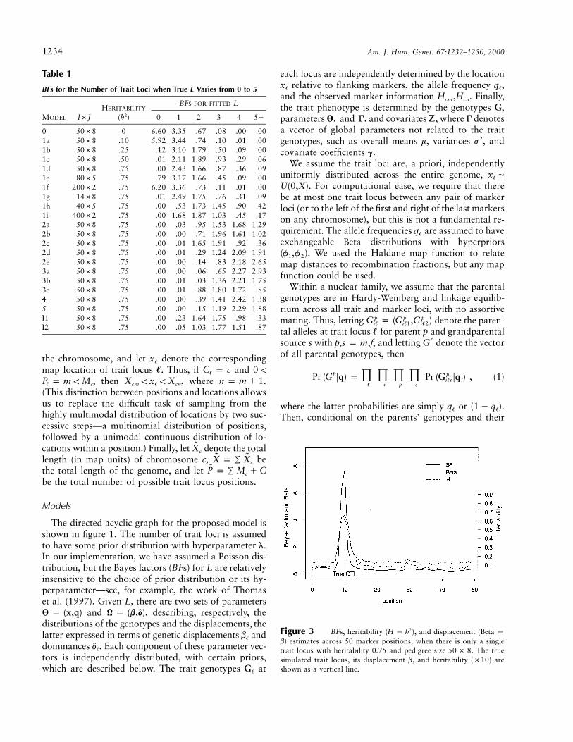
Figure 3 BFs, heritability ( ), and displacement (Beta p2H p hb) estimates across 50 marker positions, when there is only a singletrait locus with heritability 0.75 and pedigree size . The true50 # 8simulated trait locus, its displacement b, and heritability (#10) areshown as a vertical line.
the chromosome, and let denote the correspondingx�
map location of trait locus . Thus, if and� C p c 0 !�
, then , where .P p m ! M X ! x ! X n p m � 1� c cm � cn
(This distinction between positions and locations allowsus to replace the difficult task of sampling from thehighly multimodal distribution of locations by two suc-cessive steps—a multinomial distribution of positions,followed by a unimodal continuous distribution of lo-cations within a position.) Finally, let denote the totalXc
length (in map units) of chromosome c, be˜ ˜X p � Xc
the total length of the genome, and let P p � M � Cc
be the total number of possible trait locus positions.
Models
The directed acyclic graph for the proposed model isshown in figure 1. The number of trait loci is assumedto have some prior distribution with hyperparameter l.In our implementation, we have assumed a Poisson dis-tribution, but the Bayes factors (BFs) for L are relativelyinsensitive to the choice of prior distribution or its hy-perparameter—see, for example, the work of Thomaset al. (1997). Given L, there are two sets of parameters
and , describing, respectively, theV p (x,q) Q p (b,d)distributions of the genotypes and the displacements, thelatter expressed in terms of genetic displacements andb�
dominances . Each component of these parameter vec-d�
tors is independently distributed, with certain priors,which are described below. The trait genotypes atG�
each locus are independently determined by the locationrelative to flanking markers, the allele frequency ,x q� �
and the observed marker information . Finally,H ,Hcm cn
the trait phenotype is determined by the genotypes ,Gparameters , and covariates , where G denotesV, and G Za vector of global parameters not related to the traitgenotypes, such as overall means m, variances , and2j
covariate coefficients .g
We assume the trait loci are, a priori, independentlyuniformly distributed across the entire genome, x ∼�
. For computational ease, we require that there˜U(0,X)be at most one trait locus between any pair of markerloci (or to the left of the first and right of the last markerson any chromosome), but this is not a fundamental re-quirement. The allele frequencies are assumed to haveq�
exchangeable Beta distributions with hyperpriors. We used the Haldane map function to relate(f ,f )1 2
map distances to recombination fractions, but any mapfunction could be used.
Within a nuclear family, we assume that the parentalgenotypes are in Hardy-Weinberg and linkage equilib-rium across all trait and marker loci, with no assortivemating. Thus, letting denote the paren-p p pG p (G ,G )i� i�1 i�2
tal alleles at trait locus for parent p and grandparental�source s with and letting denote the vectorPp,s p m,f, Gof all parental genotypes, then
P pPr (G Fq) p � � � � Pr (G Fq ) , (1)i�s l� i p s
where the latter probabilities are simply or .q (1 � q )� �
Then, conditional on the parents’ genotypes and their
Lee and Thomas: MCMC Approaches for Mapping Genes in Oligogenic Mode 1235
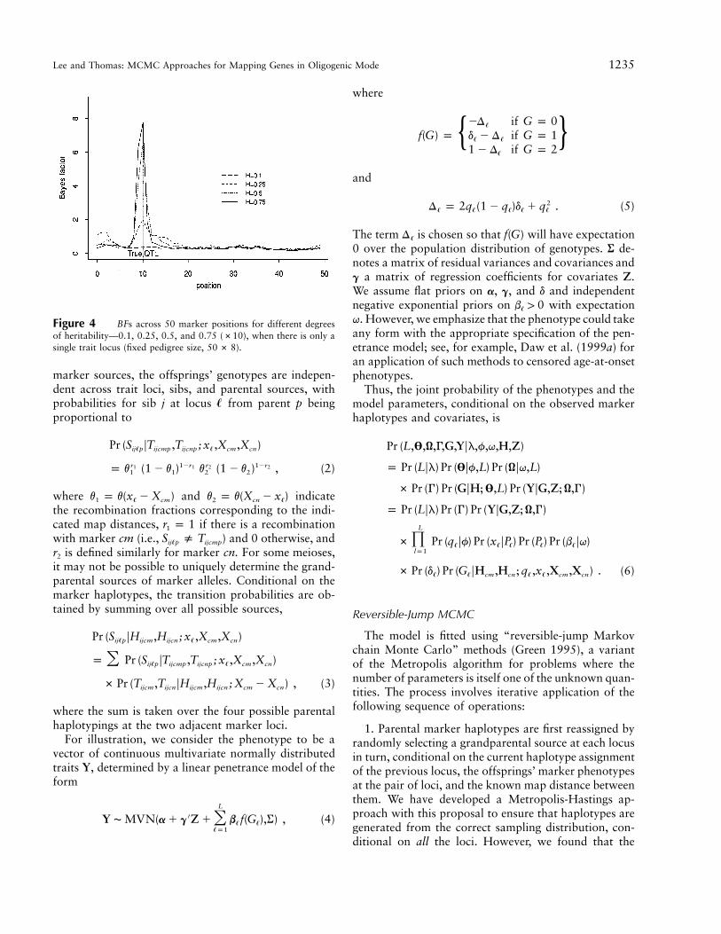
Figure 4 BFs across 50 marker positions for different degreesof heritability—0.1, 0.25, 0.5, and 0.75 (#10), when there is only asingle trait locus (fixed pedigree size, ).50 # 8
marker sources, the offsprings’ genotypes are indepen-dent across trait loci, sibs, and parental sources, withprobabilities for sib j at locus from parent p being�proportional to
Pr (S FT ,T ; x ,X ,X )ij�p ijcmp ijcnp � cm cn
r 1�r r 1�r1 1 2 2p v (1 � v ) v (1 � v ) , (2)1 1 2 2
where and indicatev p v(x � X ) v p v(X � x )1 � cm 2 cn �
the recombination fractions corresponding to the indi-cated map distances, if there is a recombinationr p 11
with marker cm (i.e., ) and 0 otherwise, andS ( Tij�p ijcmp
is defined similarly for marker cn. For some meioses,r2
it may not be possible to uniquely determine the grand-parental sources of marker alleles. Conditional on themarker haplotypes, the transition probabilities are ob-tained by summing over all possible sources,
Pr (S FH ,H ; x ,X ,X )ij�p ijcm ijcn � cm cn
p Pr (S FT ,T ; x ,X ,X )� ij�p ijcmp ijcnp � cm cn
# Pr (T ,T FH ,H ; X � X ) , (3)ijcm ijcn ijcm ijcn cm cn
where the sum is taken over the four possible parentalhaplotypings at the two adjacent marker loci.
For illustration, we consider the phenotype to be avector of continuous multivariate normally distributedtraits , determined by a linear penetrance model of theYform
L
′Y ∼ MVN(a � g Z � b f(G ),S) , (4)� � ��p1
where
�D if G p 0�
f(G) p d � D if G p 1� �{ }1 � D if G p 2�
and
2D p 2q (1 � q )d � q . (5)� � � � �
The term is chosen so that will have expectationD f(G)�
0 over the population distribution of genotypes. de-S
notes a matrix of residual variances and covariances anda matrix of regression coefficients for covariates .g Z
We assume flat priors on , , and d and independenta g
negative exponential priors on with expectationb 1 0�
q. However, we emphasize that the phenotype could takeany form with the appropriate specification of the pen-etrance model; see, for example, Daw et al. (1999a) foran application of such methods to censored age-at-onsetphenotypes.
Thus, the joint probability of the phenotypes and themodel parameters, conditional on the observed markerhaplotypes and covariates, is
Pr (L,V,Q,G,G,YFl,f,q,H,Z)
p Pr (LFl) Pr (VFf,L) Pr (QFq,L)
# Pr (G) Pr (GFH; V,L) Pr (YFG,Z; Q,G)
p Pr (LFl) Pr (G) Pr (YFG,Z; Q,G)L
#� Pr (q Ff) Pr (x FP ) Pr (P ) Pr (b Fq)� � � � �lp1
# Pr (d ) Pr (G FH ,H ; q ,x ,X ,X ) . (6)� � cm cn � � cm cn
Reversible-Jump MCMC
The model is fitted using “reversible-jump Markovchain Monte Carlo” methods (Green 1995), a variantof the Metropolis algorithm for problems where thenumber of parameters is itself one of the unknown quan-tities. The process involves iterative application of thefollowing sequence of operations:
1. Parental marker haplotypes are first reassigned byrandomly selecting a grandparental source at each locusin turn, conditional on the current haplotype assignmentof the previous locus, the offsprings’ marker phenotypesat the pair of loci, and the known map distance betweenthem. We have developed a Metropolis-Hastings ap-proach with this proposal to ensure that haplotypes aregenerated from the correct sampling distribution, con-ditional on all the loci. However, we found that the
1236 Am. J. Hum. Genet. 67:1232–1250, 2000
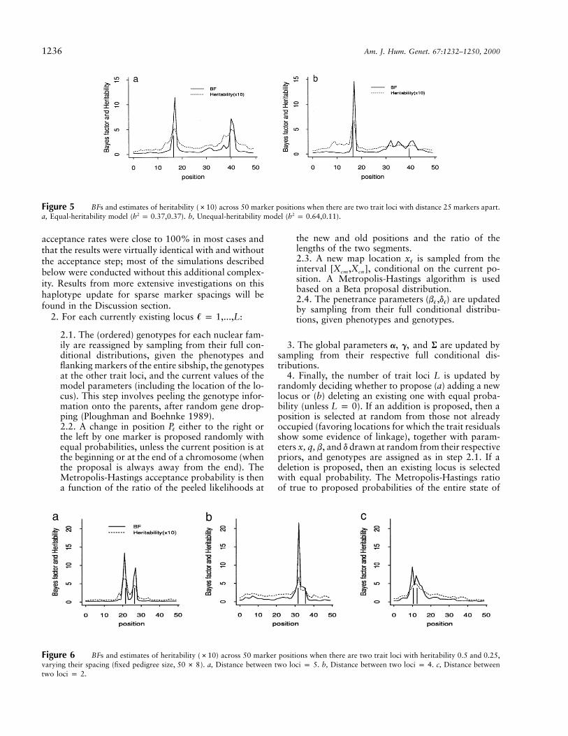
Figure 5 BFs and estimates of heritability (#10) across 50 marker positions when there are two trait loci with distance 25 markers apart.a, Equal-heritability model ( ). b, Unequal-heritability model ( ).2 2h p 0.37,0.37 h p 0.64,0.11
Figure 6 BFs and estimates of heritability (#10) across 50 marker positions when there are two trait loci with heritability 0.5 and 0.25,varying their spacing (fixed pedigree size, ). a, Distance between two loci p 5. b, Distance between two loci p 4. c, Distance between50 # 8two loci p 2.
acceptance rates were close to 100% in most cases andthat the results were virtually identical with and withoutthe acceptance step; most of the simulations describedbelow were conducted without this additional complex-ity. Results from more extensive investigations on thishaplotype update for sparse marker spacings will befound in the Discussion section.
2. For each currently existing locus :� p 1,...,L
2.1. The (ordered) genotypes for each nuclear fam-ily are reassigned by sampling from their full con-ditional distributions, given the phenotypes andflanking markers of the entire sibship, the genotypesat the other trait loci, and the current values of themodel parameters (including the location of the lo-cus). This step involves peeling the genotype infor-mation onto the parents, after random gene drop-ping (Ploughman and Boehnke 1989).2.2. A change in position either to the right orP�
the left by one marker is proposed randomly withequal probabilities, unless the current position is atthe beginning or at the end of a chromosome (whenthe proposal is always away from the end). TheMetropolis-Hastings acceptance probability is thena function of the ratio of the peeled likelihoods at
the new and old positions and the ratio of thelengths of the two segments.2.3. A new map location is sampled from thex�
interval , conditional on the current po-[X ,X ]cm cn
sition. A Metropolis-Hastings algorithm is usedbased on a Beta proposal distribution.2.4. The penetrance parameters are updated(b ,d )� �
by sampling from their full conditional distribu-tions, given phenotypes and genotypes.
3. The global parameters are updated bya, g, and Ssampling from their respective full conditional dis-tributions.
4. Finally, the number of trait loci L is updated byrandomly deciding whether to propose (a) adding a newlocus or (b) deleting an existing one with equal proba-bility (unless ). If an addition is proposed, then aL p 0position is selected at random from those not alreadyoccupied (favoring locations for which the trait residualsshow some evidence of linkage), together with param-eters x, q, b, and d drawn at random from their respectivepriors, and genotypes are assigned as in step 2.1. If adeletion is proposed, then an existing locus is selectedwith equal probability. The Metropolis-Hastings ratioof true to proposed probabilities of the entire state of
Lee and Thomas: MCMC Approaches for Mapping Genes in Oligogenic Mode 1237
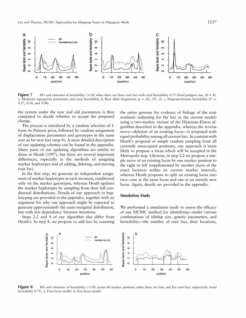
Figure 7 BFs and estimates of heritability (#10) when there are three trait loci with total heritability 0.75 (fixed pedigree size, ).50 # 8a, Moderate segregation parameters and same heritability. b, Rare allele frequencies ( ). c, Disproportionate heritability ( 2q p .02, .05, .2 h p
).0.57, 0.14, and 0.04
Figure 8 BFs and estimates of heritability (#10) across 60 marker positions when there are four and five trait loci, respectively (totalheritability 0.75). a, Four-locus model. b, Five-locus model.
the system under the new and old parameters is thencomputed to decide whether to accept the proposedchange.
The process is initialized by a random selection of Lfrom its Poisson prior, followed by random assignmentof displacement parameters and genotypes in the sameway as for new loci (step 4). A more detailed descriptionof our updating schemes can be found in the appendix.Many parts of our updating algorithms are similar tothose in Heath (1997), but there are several importantdifferences, especially in the methods of assigningmarker haplotypes and of adding, deleting, and movingtrait loci.
In the first step, we generate an independent assign-ment of marker haplotypes at each iteration, conditionalonly on the marker genotypes, whereas Heath updatesthe marker haplotypes by sampling from their full con-ditional distributions. Details of our approach to hap-lotyping are provided in the appendix, together with anargument for why our approach might be expected togenerate approximately the same marginal distribution,but with less dependency between iterations.
Steps 2.2 and 4 of our algorithm also differ fromHeath’s. In step 4, we propose to add loci by scanning
the entire genome for evidence of linkage of the traitresiduals (adjusting for the loci in the current model)using a two-marker variant of the Haseman-Elston al-gorithm described in the appendix, whereas the reversemove—deletion of an existing locus—is proposed withequal probability among all current loci. In contrast withHeath’s proposal of simple random sampling from allcurrently unoccupied positions, our approach is morelikely to propose a locus which will be accepted in theMetropolis step. Likewise, in step 2.2 we propose a sim-ple move of an existing locus by one marker position tothe right or left (supplemented by another move of theexact location within its current marker interval),whereas Heath proposes to split an existing locus intotwo—one at the same locus and one at an entirely newlocus. Again, details are provided in the appendix.
Simulation Study
We performed a simulation study to assess the efficacyof our MCMC method for identifying—under variouscombinations of sibship size, genetic parameters, andheritability—the number of trait loci, their locations,
1238 Am. J. Hum. Genet. 67:1232–1250, 2000
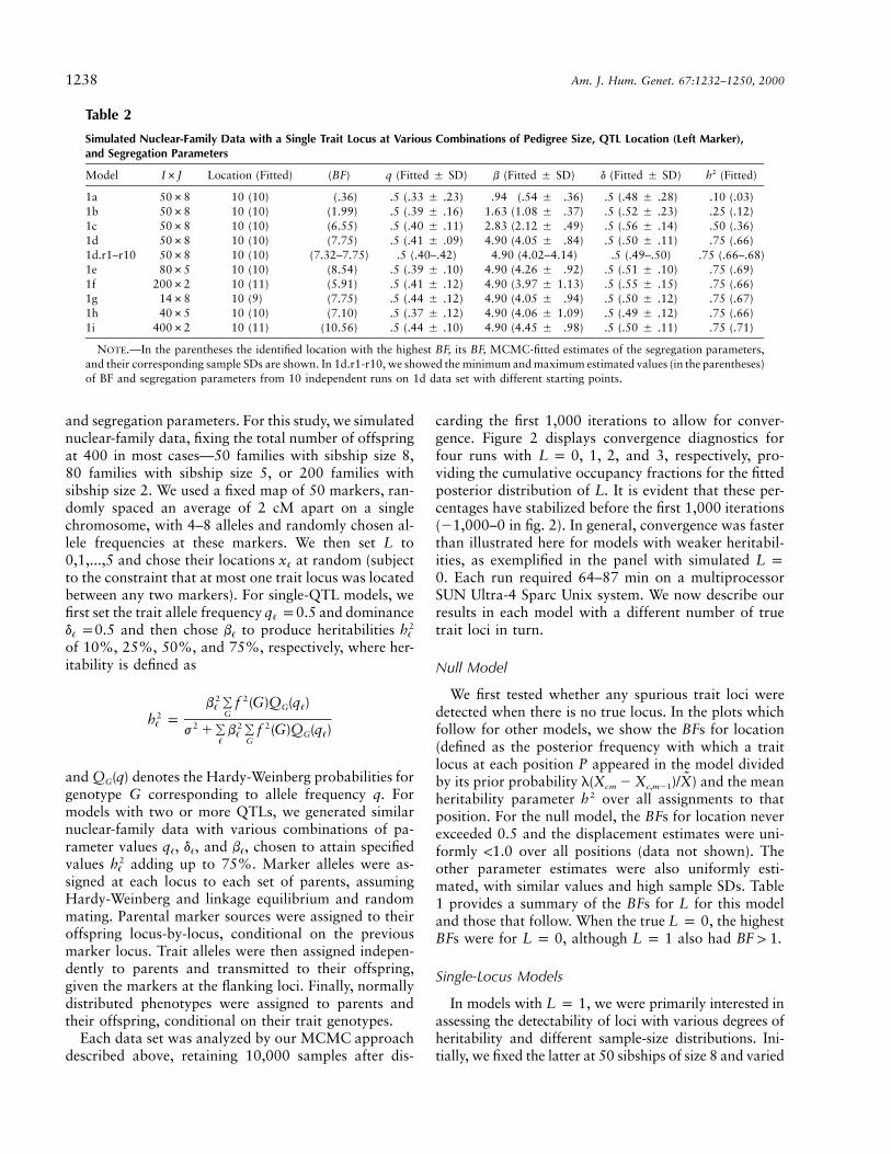
Table 2
Simulated Nuclear-Family Data with a Single Trait Locus at Various Combinations of Pedigree Size, QTL Location (Left Marker),and Segregation Parameters
Model I#J Location (Fitted) (BF) q (Fitted � SD) b (Fitted � SD) d (Fitted � SD) (Fitted)2h
1a 50#8 10 (10) (.36) .5 (.33 � .23) .94 (.54 � .36) .5 (.48 � .28) .10 (.03)1b 50#8 10 (10) (1.99) .5 (.39 � .16) 1.63 (1.08 � .37) .5 (.52 � .23) .25 (.12)1c 50#8 10 (10) (6.55) .5 (.40 � .11) 2.83 (2.12 � .49) .5 (.56 � .14) .50 (.36)1d 50#8 10 (10) (7.75) .5 (.41 � .09) 4.90 (4.05 � .84) .5 (.50 � .11) .75 (.66)1d.r1–r10 50#8 10 (10) (7.32–7.75) .5 (.40–.42) 4.90 (4.02–4.14) .5 (.49–.50) .75 (.66–.68)1e 80#5 10 (10) (8.54) .5 (.39 � .10) 4.90 (4.26 � .92) .5 (.51 � .10) .75 (.69)1f 200#2 10 (11) (5.91) .5 (.41 � .12) 4.90 (3.97 � 1.13) .5 (.55 � .15) .75 (.66)1g 14#8 10 (9) (7.75) .5 (.44 � .12) 4.90 (4.05 � .94) .5 (.50 � .12) .75 (.67)1h 40#5 10 (10) (7.10) .5 (.37 � .12) 4.90 (4.06 � 1.09) .5 (.49 � .12) .75 (.66)1i 400#2 10 (11) (10.56) .5 (.44 � .10) 4.90 (4.45 � .98) .5 (.50 � .11) .75 (.71)
NOTE.—In the parentheses the identified location with the highest BF, its BF, MCMC-fitted estimates of the segregation parameters,and their corresponding sample SDs are shown. In 1d.r1-r10, we showed the minimum and maximum estimated values (in the parentheses)of BF and segregation parameters from 10 independent runs on 1d data set with different starting points.
and segregation parameters. For this study, we simulatednuclear-family data, fixing the total number of offspringat 400 in most cases—50 families with sibship size 8,80 families with sibship size 5, or 200 families withsibship size 2. We used a fixed map of 50 markers, ran-domly spaced an average of 2 cM apart on a singlechromosome, with 4–8 alleles and randomly chosen al-lele frequencies at these markers. We then set L to
and chose their locations at random (subject0,1,...,5 x�
to the constraint that at most one trait locus was locatedbetween any two markers). For single-QTL models, wefirst set the trait allele frequency 0.5 and dominanceq p�
0.5 and then chose to produce heritabilities 2d p b h� � �
of 10%, 25%, 50%, and 75%, respectively, where her-itability is defined as
2 2b � f (G)Q (q )� G �G2h p� 2 2 2j ��b � f (G)Q (q )� G �
� G
and denotes the Hardy-Weinberg probabilities forQ (q)G
genotype G corresponding to allele frequency q. Formodels with two or more QTLs, we generated similarnuclear-family data with various combinations of pa-rameter values , , and , chosen to attain specifiedq d b� � �
values adding up to 75%. Marker alleles were as-2h�
signed at each locus to each set of parents, assumingHardy-Weinberg and linkage equilibrium and randommating. Parental marker sources were assigned to theiroffspring locus-by-locus, conditional on the previousmarker locus. Trait alleles were then assigned indepen-dently to parents and transmitted to their offspring,given the markers at the flanking loci. Finally, normallydistributed phenotypes were assigned to parents andtheir offspring, conditional on their trait genotypes.
Each data set was analyzed by our MCMC approachdescribed above, retaining 10,000 samples after dis-
carding the first 1,000 iterations to allow for conver-gence. Figure 2 displays convergence diagnostics forfour runs with and 3, respectively, pro-L p 0, 1, 2,viding the cumulative occupancy fractions for the fittedposterior distribution of L. It is evident that these per-centages have stabilized before the first 1,000 iterations(�1,000–0 in fig. 2). In general, convergence was fasterthan illustrated here for models with weaker heritabil-ities, as exemplified in the panel with simulated L p. Each run required 64–87 min on a multiprocessor0
SUN Ultra-4 Sparc Unix system. We now describe ourresults in each model with a different number of truetrait loci in turn.
Null Model
We first tested whether any spurious trait loci weredetected when there is no true locus. In the plots whichfollow for other models, we show the BFs for location(defined as the posterior frequency with which a traitlocus at each position P appeared in the model dividedby its prior probability ) and the mean˜l(X � X )/Xcm c,m�1
heritability parameter over all assignments to that2hposition. For the null model, the BFs for location neverexceeded 0.5 and the displacement estimates were uni-formly !1.0 over all positions (data not shown). Theother parameter estimates were also uniformly esti-mated, with similar values and high sample SDs. Table1 provides a summary of the BFs for L for this modeland those that follow. When the true , the highestL p 0BFs were for , although also had .L p 0 L p 1 BF 1 1
Single-Locus Models
In models with , we were primarily interested inL p 1assessing the detectability of loci with various degrees ofheritability and different sample-size distributions. Ini-tially, we fixed the latter at 50 sibships of size 8 and varied
Lee and Thomas: MCMC Approaches for Mapping Genes in Oligogenic Mode 1239
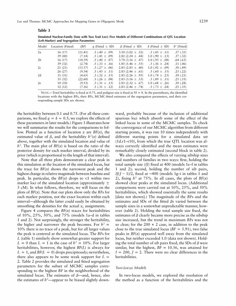
Table 3
Simulated Nuclear-Family Data with Two Trait Loci: Five Models of Different Combinations of QTL Location(Left-Marker) and Segregation Parameters
Model Location (Fitted) (BF) q (Fitted � SD) b (Fitted � SD) d (Fitted � SD) (Fitted)2h
2a 16 (17) (11.41) .5 (.40 � .09) 3.50 (3.02 � .52) .5 (.45 � .11) .37 (.35)39 (40) (7.14) .5 (.41 � .09) 2.82 (2.24 � .44) 1.0 (.90 � .13) .37 (.32)
2b 16 (17) (14.59) .5 (.40 � .07) 3.70 (3.16 � .47) 1.0 (.93 � .08) .64 (.63)39 (32) (2.74) .5 (.33 � .16) 1.85 (1.46 � .55) .5 (.36 � .24) .11 (.06)
2c 21 (21) (13.37) .3 (.27 � .06) 2.83 (2.85 � .40) 1.0 (.92 � .09) .50 (.49)26 (27) (9.34) .5 (.43 � .11) 2.83 (2.46 � .61) .5 (.60 � .15) .25 (.22)
2d 31 (31) (4.65) .3 (.32 � .15) 2.83 (2.26 � .95) 1.0 (.74 � .23) .50 (.21)35 (32) (22.60) .5 (.26 � .08) 2.83 (3.16 � .53) .5 (.89 � .11) .25 (.53)
2e 10 (10) (9.53) .3 (.31 � .13) 2.83 (2.32 � .67) 1.0 (.68 � .26) .50 (.28)12 (12) (7.16) .5 (.31 � .12) 2.83 (2.46 � .74) .5 (.73 � .24) .25 (.35)
NOTE.—Total heritability is fixed at 0.75, and pedigree size is fixed at . In the parentheses, the identified50 # 8locations with the highest BFs, their BFs, MCMC-fitted estimates of the segregation parameters, and their cor-responding sample SDs are shown.
the heritability between 0.1 and 0.75. (For all these com-parisons, we fixed ; we explore the effects ofq p d p 0.5these parameters in later models.) Figure 3 illustrates howwe will summarize the results for the comparisons to fol-low. Plotted as a function of location x are , theBF(x)estimated value of b, and the heritability defined2h (x)above, together with the simulated location and value of
. The main plot of is based on the ratio of the2h BF(x)posterior density for each marker interval, divided by itsprior (which is proportional to the length of that interval).
Note that all three plots demonstrate a clear peak inthis simulation at the location of the simulated locus, butthe trace for shows the narrowest peak and theBF(x)highest change in relative magnitude between baseline andpeak. In particular, the drops to !1 within twoBF(x)marker loci of the simulated location (approximately �
cM). In what follows, therefore, we will focus on the5plots of . Note that our plots show only the BFs forBF(x)each marker position, not the exact location within eachinterval—although the latter could easily be obtained bysmoothing the densities for the actual assignments.x�
Figure 4 compares the traces for heritabilitiesBF(x)of 10%, 25%, 50%, and 75% (models 1a–d in tables1 and 2). Not surprisingly, the stronger the heritability,the higher and narrower the peak becomes. For 2h p
there is no trace of a peak, but for all larger values10%the peak is centered at the simulated locus. The BFs forL (table 1) similarly show somewhat greater support for
than in the case of . For larger2L p 0 L p 1 h p 10%heritabilities, however, the highest is always forBF(L)
, and drops precipitously; nevertheless,L p 1 BF(L p 0)there also appears to be some weak support for L p. Table 2 provides the simulated and fitted segregation2
parameters for the subset of MCMC samples corre-sponding to the highest BF in the neighborhood of thesimulated locus. The estimates of b—and, hence, alsothe estimates of —appear to be biased slightly down-2h
ward, probably because of the inclusion of additionalspurious loci which absorb some of the effect of thelinked locus in some of the MCMC samples. To checkthe convergence of our MCMC algorithm from differentstarting points, it was run 10 times independently withdifferent starting points for a simulated data set(1d.r1–r10), from which the true QTL location was al-ways correctly identified and the mean estimates wereremarkably closely estimated (second block in table 2).
We also compared the effects of varying sibship sizesand numbers of families in two ways: first, holding thetotal sample size (IJ) fixed at 400 (models 1e–f in tables1 and 2); second, holding the number of sib pairs,
, fixed at ∼400 (models 1g–i in tables 1 andIJ(J � 1)/22), fixing at 75%. In all cases, the plots of2h BF(x)showed clear peaks at the simulated locus. (Additionalcomparisons were carried out at 10%, 25%, and 50%heritabilities, which showed essentially the same results[data not shown].) The magnitude of the BFs and theestimates and SDs of the fitted bs varied between thesample sizes in a somewhat unpredictable manner, how-ever (table 2). Holding the total sample size fixed, theestimates of b clearly became more precise as the sibshipsize increased, but the trend in maximum BFs was notso clear; for the case, in addition to the peak200 # 2close to the true simulated locus ( ), two falseBF p 5.91peaks in appeared well away from the simulatedBF(x)locus, but neither exceeded 1.0 (data not shown). Hold-ing the total number of sib pairs fixed, the SDs of b weresimilar, but the highest, , was attained forBF p 10.56
. There were no clear differences in theI p 200, J p 2heritabilities.
Two-Locus Models
In two-locus models, we explored the resolution ofthe method as a function of the heritabilities and the
1240 Am. J. Hum. Genet. 67:1232–1250, 2000
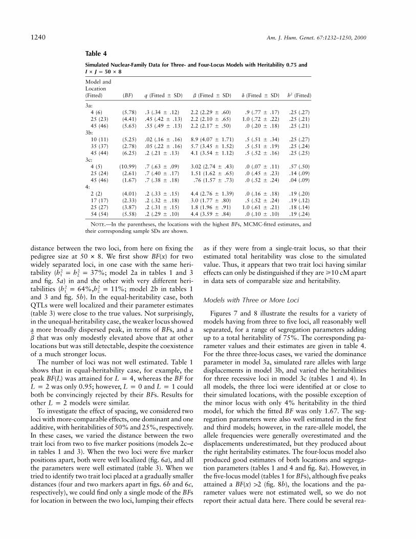
Table 4
Simulated Nuclear-Family Data for Three- and Four-Locus Models with Heritability and0.75I # J p 50 # 8
Model andLocation(Fitted) (BF) q (Fitted � SD) b (Fitted � SD) d (Fitted � SD) (Fitted)2h
3a:4 (6) (5.78) .3 (.34 � .12) 2.2 (2.29 � .60) .9 (.77 � .17) .25 (.27)25 (23) (4.41) .45 (.42 � .13) 2.2 (2.10 � .65) 1.0 (.72 � .22) .25 (.21)45 (46) (5.65) .55 (.49 � .13) 2.2 (2.17 � .50) .0 (.20 � .18) .25 (.21)
3b:10 (11) (5.25) .02 (.16 � .16) 8.9 (4.07 � 1.71) .5 (.51 � .34) .25 (.27)35 (37) (2.78) .05 (.22 � .16) 5.7 (3.45 � 1.52) .5 (.51 � .19) .25 (.24)45 (44) (6.25) .2 (.21 � .13) 4.1 (3.54 � 1.12) .5 (.52 � .16) .25 (.25)
3c:4 (5) (10.99) .7 (.63 � .09) 3.02 (2.74 � .43) .0 (.07 � .11) .57 (.50)25 (24) (2.61) .7 (.40 � .17) 1.51 (1.62 � .65) .0 (.45 � .23) .14 (.09)45 (46) (1.67) .7 (.38 � .18) .76 (1.57 � .73) .0 (.52 � .24) .04 (.09)
4:2 (2) (4.01) .2 (.33 � .15) 4.4 (2.76 � 1.39) .0 (.16 � .18) .19 (.20)17 (17) (2.33) .2 (.32 � .18) 3.0 (1.77 � .80) .5 (.52 � .24) .19 (.12)25 (27) (3.87) .2 (.31 � .15) 1.8 (1.96 � .91) 1.0 (.61 � .21) .18 (.14)54 (54) (5.58) .2 (.29 � .10) 4.4 (3.59 � .84) .0 (.10 � .10) .19 (.24)
NOTE.—In the parentheses, the locations with the highest BFs, MCMC-fitted estimates, andtheir corresponding sample SDs are shown.
distance between the two loci, from here on fixing thepedigree size at . We first show for two50 # 8 BF(x)widely separated loci, in one case with the same heri-tability ( ; model 2a in tables 1 and 32 2h p h p 37%1 2
and fig. 5a) in and the other with very different heri-tabilities ( ; model 2b in tables 12 2h p 64%,h p 11%1 2
and 3 and fig. 5b). In the equal-heritability case, bothQTLs were well localized and their parameter estimates(table 3) were close to the true values. Not surprisingly,in the unequal-heritability case, the weaker locus showeda more broadly dispersed peak, in terms of BFs, and a
that was only modestly elevated above that at otherb
locations but was still detectable, despite the coexistenceof a much stronger locus.
The number of loci was not well estimated. Table 1shows that in equal-heritability case, for example, thepeak was attained for , whereas the BF forBF(L) L p 4
was only 0.95; however, and couldL p 2 L p 0 L p 1both be convincingly rejected by their BFs. Results forother models were similar.L p 2
To investigate the effect of spacing, we considered twoloci with more-comparable effects, one dominant and oneadditive, with heritabilities of 50% and 25%, respectively.In these cases, we varied the distance between the twotrait loci from two to five marker positions (models 2c–ein tables 1 and 3). When the two loci were five markerpositions apart, both were well localized (fig. 6a), and allthe parameters were well estimated (table 3). When wetried to identify two trait loci placed at a gradually smallerdistances (four and two markers apart in figs. 6b and 6c,respectively), we could find only a single mode of the BFsfor location in between the two loci, lumping their effects
as if they were from a single-trait locus, so that theirestimated total heritability was close to the simulatedvalue. Thus, it appears that two trait loci having similareffects can only be distinguished if they are �10 cM apartin data sets of comparable size and heritability.
Models with Three or More Loci
Figures 7 and 8 illustrate the results for a variety ofmodels having from three to five loci, all reasonably wellseparated, for a range of segregation parameters addingup to a total heritability of 75%. The corresponding pa-rameter values and their estimates are given in table 4.For the three three-locus cases, we varied the dominanceparameter in model 3a, simulated rare alleles with largedisplacements in model 3b, and varied the heritabilitiesfor three recessive loci in model 3c (tables 1 and 4). Inall models, the three loci were identified at or close totheir simulated locations, with the possible exception ofthe minor locus with only 4% heritability in the thirdmodel, for which the fitted BF was only 1.67. The seg-regation parameters were also well estimated in the firstand third models; however, in the rare-allele model, theallele frequencies were generally overestimated and thedisplacements underestimated, but they produced aboutthe right heritability estimates. The four-locus model alsoproduced good estimates of both locations and segrega-tion parameters (tables 1 and 4 and fig. 8a). However, inthe five-locus model (tables 1 for BFs), although five peaksattained a 12 (fig. 8b), the locations and the pa-BF(x)rameter values were not estimated well, so we do notreport their actual data here. There could be several rea-
Lee and Thomas: MCMC Approaches for Mapping Genes in Oligogenic Mode 1241
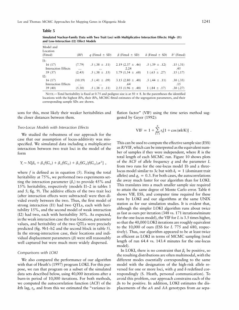
Table 5
Simulated Nuclear-Family Data with Two Trait Loci with Multiplicative Interaction Effects: High- (I1)and Low-Interaction (I2) Effect Models
Model andLocation(Fitted) (BF) q (Fitted � SD) b (Fitted � SD) d (Fitted � SD) (Fitted)2h
I1:16 (17) (7.79) .5 (.38 � .11) 2.19 (2.37 � .46) .5 (.39 � .12) .15 (.31)Interaction Effects … … 2.24 … .4539 (37) (2.45) .5 (.38 � .15) 1.79 (1.54 � .68) 1 (.63 � .27) .15 (.17)
I2:16 (17) (10.19) .5 (.41 � .09) 3.15 (2.80 � .48) .5 (.44 � .11) .30 (.35)Interaction Effects … … .64 .1539 (40) (5.30) .5 (.38 � .11) 2.55 (1.96 � .48) 1 (.84 � .17) .30 (.27)
NOTE.—Total heritability is fixed at 0.75 and pedigree size is at . In the parentheses the identified50 # 8locations with the highest BFs, their BFs, MCMC-fitted estimates of the segregation parameters, and theircorresponding sample SDs are shown.
sons for this, most likely their weaker heritabilities andthe closer distances between them.
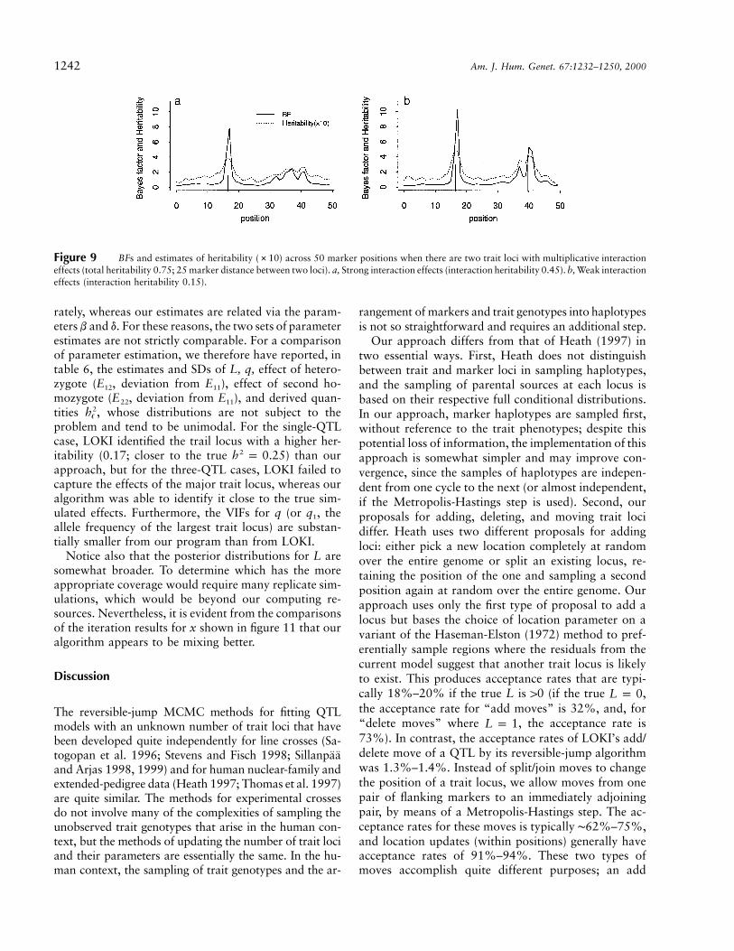
Two-Locus Models with Interaction Effects
We studied the robustness of our approach for thecase that our assumption of locus-additivity was mis-specified. We simulated data including a multiplicativeinteraction between two trait loci in the model of theform
2Y ∼ N[b � b f(G ) � b f(G ) � b f(G )f(G ),j ] ,i 0 1 i1 2 i2 3 i1 i2
where f is defined as in equation (5). Fixing the totalheritability at 75%, we performed two experiments set-ting the interaction parameter ( ) to provide 45% andb3
15% heritability, respectively (models I1–2 in tables 1and 5; fig. 9). The additive effects of the two trait loci(after interaction effects were subtracted) were then di-vided evenly between the two. Thus, the first model ofstrong interaction (I1) had two QTLs, each with heri-tability 15%, and the second model of weak interaction(I2) had two, each with heritability 30%. As expected,in the weak interaction case the true locations, parametervalues, and heritability of the two QTLs were preciselypredicted (fig. 9b1–b2 and the second block in table 5).In the strong-interaction case, their locations and indi-vidual displacement parameters (b) were still reasonablywell captured but were much more widely dispersed.
Comparisons with LOKI
We also compared the performance of our algorithmwith that of Heath’s (1997) program LOKI. For this pur-pose, we ran that program on a subset of the simulateddata sets described below, using 40,000 iterations after aburn-in period of 10,000 iterations. For both methods,we computed the autocorrelation function (ACF) of thekth lag, , and from this we estimated the “variance in-rk
flation factor” (VIF) using the time series method sug-gested by Geyer (1992):
K
VIF p 1 � r [1 � cos (pk/K)] .� kkp1
This can be used to compute the effective sample size (ESS)as , which can be interpreted as the equivalent num-R/VIFber of samples if they were independent, where R is thetotal length of each MCMC run. Figure 10 shows plotsof the ACF of allele frequency q and the parameter Lfrom two runs for the one-locus model 1b and a three-locus model similar to 3c but with (dominant traitd p 1�
alleles) and . For both cases, the autocorrelationsq p 0.3�
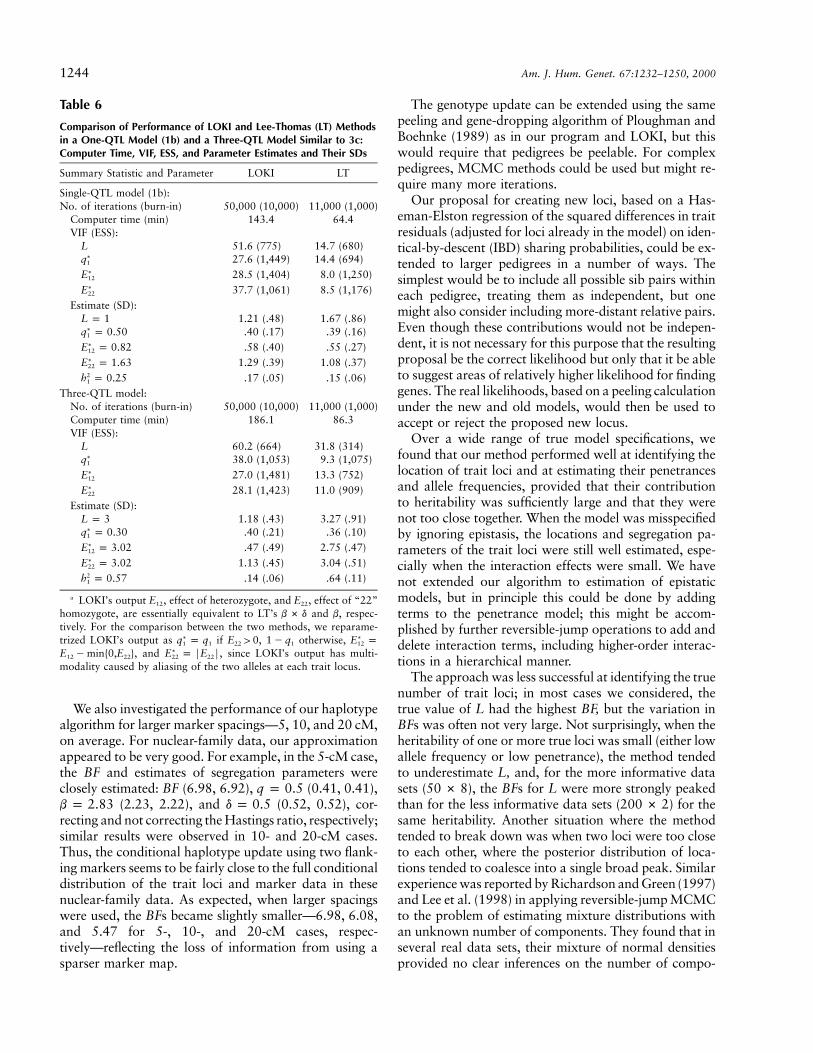
die away much faster for our algorithm than for LOKI.This translates into a much smaller sample size requiredto attain the same degree of Monte Carlo error. Table 6shows VIF, ESS, and computer time required for theseruns by LOKI and our algorithms at the same UNIXstation as for our simulation studies. It is evident that,although the simpler LOKI algorithm runs about twiceas fast as ours per iteration (348 vs. 171 iterations/minutefor the one-locus model), the VIF for L is 3.5 times higher,so that the 40,000 LOKI iterations are roughly equivalentto the 10,000 of ours (ESS for L 775 and 680, respec-tively). Thus, our algorithm appeared to be at least twiceas efficient as LOKI in terms of MCMC sampling (totallength of run 64.4 vs. 143.4 minutes for the one-locusmodel).
In LOKI, there is no constraint that be positive, sob�
the resulting distributions are often multimodal, with thedifferent modes essentially corresponding to the samemodel with the designation of the high-risk allele re-versed for one or more loci, with q and d redefined cor-respondingly (S. Heath, personal communication). Toavoid this problem, our approach constrains each of thebs to be positive. In addition, LOKI estimates the dis-placements of the aA and AA genotypes from aa sepa-
1242 Am. J. Hum. Genet. 67:1232–1250, 2000
Figure 9 BFs and estimates of heritability (#10) across 50 marker positions when there are two trait loci with multiplicative interactioneffects (total heritability 0.75; 25 marker distance between two loci). a, Strong interaction effects (interaction heritability 0.45). b, Weak interactioneffects (interaction heritability 0.15).
rately, whereas our estimates are related via the param-eters b and d. For these reasons, the two sets of parameterestimates are not strictly comparable. For a comparisonof parameter estimation, we therefore have reported, intable 6, the estimates and SDs of L, q, effect of hetero-zygote ( , deviation from ), effect of second ho-E E12 11
mozygote ( , deviation from ), and derived quan-E E22 11
tities , whose distributions are not subject to the2h�
problem and tend to be unimodal. For the single-QTLcase, LOKI identified the trail locus with a higher her-itability (0.17; closer to the true ) than our2h p 0.25approach, but for the three-QTL cases, LOKI failed tocapture the effects of the major trait locus, whereas ouralgorithm was able to identify it close to the true sim-ulated effects. Furthermore, the VIFs for q (or , theq1
allele frequency of the largest trait locus) are substan-tially smaller from our program than from LOKI.
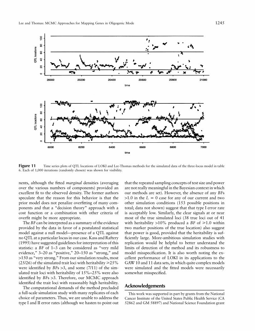
Notice also that the posterior distributions for L aresomewhat broader. To determine which has the moreappropriate coverage would require many replicate sim-ulations, which would be beyond our computing re-sources. Nevertheless, it is evident from the comparisonsof the iteration results for x shown in figure 11 that ouralgorithm appears to be mixing better.
Discussion
The reversible-jump MCMC methods for fitting QTLmodels with an unknown number of trait loci that havebeen developed quite independently for line crosses (Sa-togopan et al. 1996; Stevens and Fisch 1998; Sillanpaaand Arjas 1998, 1999) and for human nuclear-family andextended-pedigree data (Heath 1997; Thomas et al. 1997)are quite similar. The methods for experimental crossesdo not involve many of the complexities of sampling theunobserved trait genotypes that arise in the human con-text, but the methods of updating the number of trait lociand their parameters are essentially the same. In the hu-man context, the sampling of trait genotypes and the ar-
rangement of markers and trait genotypes into haplotypesis not so straightforward and requires an additional step.
Our approach differs from that of Heath (1997) intwo essential ways. First, Heath does not distinguishbetween trait and marker loci in sampling haplotypes,and the sampling of parental sources at each locus isbased on their respective full conditional distributions.In our approach, marker haplotypes are sampled first,without reference to the trait phenotypes; despite thispotential loss of information, the implementation of thisapproach is somewhat simpler and may improve con-vergence, since the samples of haplotypes are indepen-dent from one cycle to the next (or almost independent,if the Metropolis-Hastings step is used). Second, ourproposals for adding, deleting, and moving trait locidiffer. Heath uses two different proposals for addingloci: either pick a new location completely at randomover the entire genome or split an existing locus, re-taining the position of the one and sampling a secondposition again at random over the entire genome. Ourapproach uses only the first type of proposal to add alocus but bases the choice of location parameter on avariant of the Haseman-Elston (1972) method to pref-erentially sample regions where the residuals from thecurrent model suggest that another trait locus is likelyto exist. This produces acceptance rates that are typi-cally 18%–20% if the true L is 10 (if the true ,L p 0the acceptance rate for “add moves” is 32%, and, for“delete moves” where , the acceptance rate isL p 173%). In contrast, the acceptance rates of LOKI’s add/delete move of a QTL by its reversible-jump algorithmwas 1.3%–1.4%. Instead of split/join moves to changethe position of a trait locus, we allow moves from onepair of flanking markers to an immediately adjoiningpair, by means of a Metropolis-Hastings step. The ac-ceptance rates for these moves is typically ∼62%–75%,and location updates (within positions) generally haveacceptance rates of 91%–94%. These two types ofmoves accomplish quite different purposes; an add
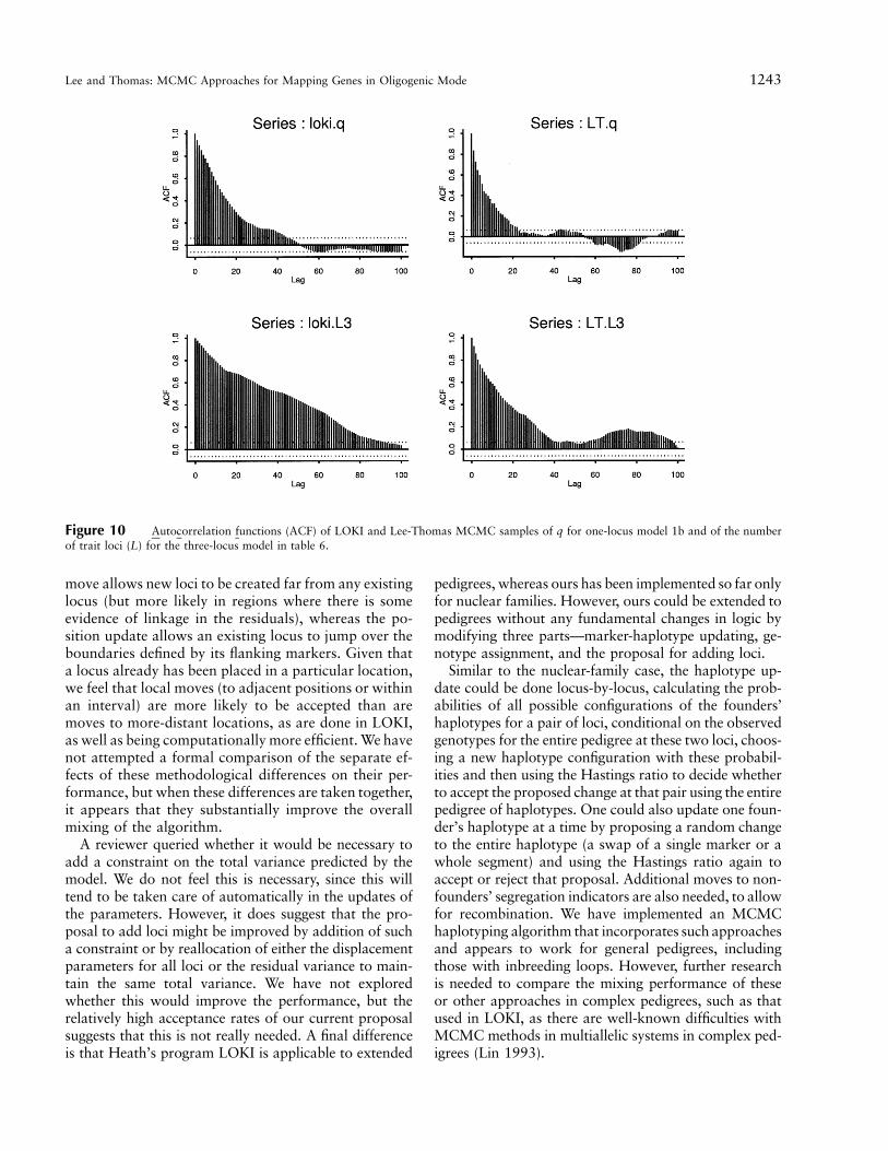
Lee and Thomas: MCMC Approaches for Mapping Genes in Oligogenic Mode 1243
Figure 10 Autocorrelation functions (ACF) of LOKI and Lee-Thomas MCMC samples of q for one-locus model 1b and of the numberof trait loci (L) for the three-locus model in table 6.
move allows new loci to be created far from any existinglocus (but more likely in regions where there is someevidence of linkage in the residuals), whereas the po-sition update allows an existing locus to jump over theboundaries defined by its flanking markers. Given thata locus already has been placed in a particular location,we feel that local moves (to adjacent positions or withinan interval) are more likely to be accepted than aremoves to more-distant locations, as are done in LOKI,as well as being computationally more efficient. We havenot attempted a formal comparison of the separate ef-fects of these methodological differences on their per-formance, but when these differences are taken together,it appears that they substantially improve the overallmixing of the algorithm.
A reviewer queried whether it would be necessary toadd a constraint on the total variance predicted by themodel. We do not feel this is necessary, since this willtend to be taken care of automatically in the updates ofthe parameters. However, it does suggest that the pro-posal to add loci might be improved by addition of sucha constraint or by reallocation of either the displacementparameters for all loci or the residual variance to main-tain the same total variance. We have not exploredwhether this would improve the performance, but therelatively high acceptance rates of our current proposalsuggests that this is not really needed. A final differenceis that Heath’s program LOKI is applicable to extended
pedigrees, whereas ours has been implemented so far onlyfor nuclear families. However, ours could be extended topedigrees without any fundamental changes in logic bymodifying three parts—marker-haplotype updating, ge-notype assignment, and the proposal for adding loci.
Similar to the nuclear-family case, the haplotype up-date could be done locus-by-locus, calculating the prob-abilities of all possible configurations of the founders’haplotypes for a pair of loci, conditional on the observedgenotypes for the entire pedigree at these two loci, choos-ing a new haplotype configuration with these probabil-ities and then using the Hastings ratio to decide whetherto accept the proposed change at that pair using the entirepedigree of haplotypes. One could also update one foun-der’s haplotype at a time by proposing a random changeto the entire haplotype (a swap of a single marker or awhole segment) and using the Hastings ratio again toaccept or reject that proposal. Additional moves to non-founders’ segregation indicators are also needed, to allowfor recombination. We have implemented an MCMChaplotyping algorithm that incorporates such approachesand appears to work for general pedigrees, includingthose with inbreeding loops. However, further researchis needed to compare the mixing performance of theseor other approaches in complex pedigrees, such as thatused in LOKI, as there are well-known difficulties withMCMC methods in multiallelic systems in complex ped-igrees (Lin 1993).
1244 Am. J. Hum. Genet. 67:1232–1250, 2000
Table 6
Comparison of Performance of LOKI and Lee-Thomas (LT) Methodsin a One-QTL Model (1b) and a Three-QTL Model Similar to 3c:Computer Time, VIF, ESS, and Parameter Estimates and Their SDs
Summary Statistic and Parameter LOKI LT
Single-QTL model (1b):No. of iterations (burn-in) 50,000 (10,000) 11,000 (1,000)
Computer time (min) 143.4 64.4VIF (ESS):
L 51.6 (775) 14.7 (680)∗q1 27.6 (1,449) 14.4 (694)∗E12 28.5 (1,404) 8.0 (1,250)∗E22 37.7 (1,061) 8.5 (1,176)
Estimate (SD):L p 1 1.21 (.48) 1.67 (.86)
∗q p 0.501 .40 (.17) .39 (.16)∗E p 0.8212 .58 (.40) .55 (.27)∗E p 1.6322 1.29 (.39) 1.08 (.37)2h p 0.251 .17 (.05) .15 (.06)
Three-QTL model:No. of iterations (burn-in) 50,000 (10,000) 11,000 (1,000)Computer time (min) 186.1 86.3VIF (ESS):
L 60.2 (664) 31.8 (314)∗q1 38.0 (1,053) 9.3 (1,075)∗E12 27.0 (1,481) 13.3 (752)∗E22 28.1 (1,423) 11.0 (909)
Estimate (SD):L p 3 1.18 (.43) 3.27 (.91)
∗q p 0.301 .40 (.21) .36 (.10)∗E p 3.0212 .47 (.49) 2.75 (.47)∗E p 3.0222 1.13 (.45) 3.04 (.51)2h p 0.571 .14 (.06) .64 (.11)
a LOKI’s output , effect of heterozygote, and , effect of “22”E E12 22
homozygote, are essentially equivalent to LT’s and b, respec-b # d
tively. For the comparison between the two methods, we reparame-trized LOKI’s output as if , otherwise,∗ ∗q p q E 1 0 1 � q E p1 1 22 1 12
, and , since LOKI’s output has multi-∗E � min{0,E } E p FE F12 22 22 22
modality caused by aliasing of the two alleles at each trait locus.
We also investigated the performance of our haplotypealgorithm for larger marker spacings—5, 10, and 20 cM,on average. For nuclear-family data, our approximationappeared to be very good. For example, in the 5-cM case,the BF and estimates of segregation parameters wereclosely estimated: BF (6.98, 6.92), (0.41, 0.41),q p 0.5
(2.23, 2.22), and (0.52, 0.52), cor-b p 2.83 d p 0.5recting and not correcting the Hastings ratio, respectively;similar results were observed in 10- and 20-cM cases.Thus, the conditional haplotype update using two flank-ing markers seems to be fairly close to the full conditionaldistribution of the trait loci and marker data in thesenuclear-family data. As expected, when larger spacingswere used, the BFs became slightly smaller—6.98, 6.08,and 5.47 for 5-, 10-, and 20-cM cases, respec-tively—reflecting the loss of information from using asparser marker map.
The genotype update can be extended using the samepeeling and gene-dropping algorithm of Ploughman andBoehnke (1989) as in our program and LOKI, but thiswould require that pedigrees be peelable. For complexpedigrees, MCMC methods could be used but might re-quire many more iterations.
Our proposal for creating new loci, based on a Has-eman-Elston regression of the squared differences in traitresiduals (adjusted for loci already in the model) on iden-tical-by-descent (IBD) sharing probabilities, could be ex-tended to larger pedigrees in a number of ways. Thesimplest would be to include all possible sib pairs withineach pedigree, treating them as independent, but onemight also consider including more-distant relative pairs.Even though these contributions would not be indepen-dent, it is not necessary for this purpose that the resultingproposal be the correct likelihood but only that it be ableto suggest areas of relatively higher likelihood for findinggenes. The real likelihoods, based on a peeling calculationunder the new and old models, would then be used toaccept or reject the proposed new locus.
Over a wide range of true model specifications, wefound that our method performed well at identifying thelocation of trait loci and at estimating their penetrancesand allele frequencies, provided that their contributionto heritability was sufficiently large and that they werenot too close together. When the model was misspecifiedby ignoring epistasis, the locations and segregation pa-rameters of the trait loci were still well estimated, espe-cially when the interaction effects were small. We havenot extended our algorithm to estimation of epistaticmodels, but in principle this could be done by addingterms to the penetrance model; this might be accom-plished by further reversible-jump operations to add anddelete interaction terms, including higher-order interac-tions in a hierarchical manner.
The approach was less successful at identifying the truenumber of trait loci; in most cases we considered, thetrue value of L had the highest BF, but the variation inBFs was often not very large. Not surprisingly, when theheritability of one or more true loci was small (either lowallele frequency or low penetrance), the method tendedto underestimate L, and, for the more informative datasets ( ), the BFs for L were more strongly peaked50 # 8than for the less informative data sets ( ) for the200 # 2same heritability. Another situation where the methodtended to break down was when two loci were too closeto each other, where the posterior distribution of loca-tions tended to coalesce into a single broad peak. Similarexperience was reported by Richardson and Green (1997)and Lee et al. (1998) in applying reversible-jump MCMCto the problem of estimating mixture distributions withan unknown number of components. They found that inseveral real data sets, their mixture of normal densitiesprovided no clear inferences on the number of compo-
Lee and Thomas: MCMC Approaches for Mapping Genes in Oligogenic Mode 1245
Figure 11 Time series plots of QTL locations of LOKI and Lee-Thomas methods for the simulated data of the three-locus model in table6. Each of 1,000 iterations (randomly chosen) was shown for visibility.
nents, although the fitted marginal densities (averagingover the various numbers of components) provided anexcellent fit to the observed density. The former authorsspeculate that the reason for this behavior is that theprior model does not penalize overfitting of many com-ponents and that a “decision theory” approach with acost function or a combination with other criteria ofoverfit might be more appropriate.
The BF can be interpreted as a summary of the evidenceprovided by the data in favor of a postulated statisticalmodel against a null model—presence of a QTL againstno QTL at a particular locus in our case. Kass and Raftery(1995) have suggested guidelines for interpretation of thisstatistic: a BF of 1–3 can be considered as “very mildevidence,” 3–20 as “positive,” 20–150 as “strong,” and1150 as “very strong.” From our simulation results, most(25/26) of the simulated trait loci with heritability �25%were identified by BFs 13, and some (7/11) of the sim-ulated trait loci with heritability of 15%–25% were alsoidentified by BFs 13. Therefore, our MCMC approachidentified the trait loci with reasonably high heritability.
The computational demands of the method precludeda full-scale simulation study with many replicates of eachchoice of parameters. Thus, we are unable to address thetype I and II error rates (although we hasten to point out
that the repeated sampling concepts of test size and powerare not really meaningful in the Bayesian context in whichour methods are set). However, the absence of any BFs11.0 in the case for any of our current and twoL p 0other simulation conditions (153 possible positions intotal; data not shown) suggest that that type I error rateis acceptably low. Similarly, the clear signals at or nearmost of the true simulated loci (38 true loci out of 41with heritability 110% produced a BF of �1.0 withintwo marker positions of the true location) also suggestthat power is good, provided that the heritability is suf-ficiently large. More-ambitious simulation studies withreplication would be helpful to better understand thelimits of detection of the method and its robustness tomodel misspecification. It is also worth noting the ex-cellent performance of LOKI in its applications to theGAW 10 and 11 data sets, in which quite complex modelswere simulated and the fitted models were necessarilysomewhat misspecified.
Acknowledgements
This work was supported in part by grants from the NationalCancer Institute of the United States Public Health Service (CA52862 and GM 58897) and National Science Foundation grant
1246 Am. J. Hum. Genet. 67:1232–1250, 2000
BIR 95-04393. We thank Dr. Sylvia Richardson for help in thedevelopment of the algorithm, Dr. Simon Heath for useful dis-
cussions on LOKI’s output, and the reviewers for helpful com-ments and many editorial suggestions on the manuscript.
Appendix A
MCMC Updating Procedures
Haplotype Assignment
The marker phenotypes are randomly reassigned to haplotypes at the beginning of each cycle. This is done se-quentially on each chromosome, beginning with an arbitrary assignment of the marker alleles at the first locus tograndparental sources and then conditioning the assignment of subsequent loci on the grandparental sources of theprevious locus. Let us consider two marker loci, each with four different allele types: a, b, c, d for the first locus andA, B, C, D for the second one. We then distinguish three potentially informative configurations of parental markerphenotypes at the second locus: (1) both parents heterozygous and sharing, at most, one allele; (2) one parentheterozygous; (3) parents sharing two alleles with subtypes (a) if the offspring is homozygous and (b) if the offspringis heterozygous. In each of these situations, the haplotype probabilities depend on the recombination fraction, asproducts over all the offspring of , , and . A pair of parental haplotypes is then2 2v/2 (1 � v)/2 V p [v � (1 � v) ]/2sampled with these probabilities. Grandparental sources are assigned to each of the offspring where they canTijcmp
be inferred directly by matching the alleles; for example, in configuration (1), if the parents were assigned haplotypeaA bB cD dC, then an offspring with genotype ac,AC could only be assigned haplotype aA cC with sources fF fMF # F F F(where “f” and “m” denote grandpaternal and grandmaternal sources, respectively, for the first locus, and likewisefor the second locus). Similar situations arise in configuration (3a) and for the heterozygous parent in configuration(2). In the ambiguous situations, the two possible haplotypes are assigned at random with the appropriate probabilities.For example, in configuration (2), the source for the homozygous parent would be assigned with probability v or
, depending upon the assignment at the first locus. In configuration (3b), if the parents were assigned haplotypes1 � v
aA bB cB dA, then an offspring with genotype ac,AB could be assigned either haplotype aA cB (fF fF) or haplotypeF # F F FaB cA (fM fM) with probabilities and respectively; on the other hand, if the parents were assigned2 2F F (1 � v) /2V v /2V
aA bB cA dB, the two offspring haplotypes would be assigned with equal probability.F # FAs noted by a reviewer, sampling locus by locus in this fashion does not exactly generate the correct haplotype
distribution, because we do not use the full phenotype data. Specifically, the true distribution, , can be decom-P(TFH)posed as
[T FH][T FT ,]...[T FT ,...,T ,H] ,1 2 1 L 1 L�1
but what we actually sample from is
Q(TFH) p [T FH ][T FT ,H ,H ]...P[TFT ,H ,H ]...P[T FT ,H ] .1 1 2 1 1 2 � ��1 ��1 � L L�1 L�1
The appropriate fix is to either accept or reject a new haplotyping based on the Hastings ratio, R p. However, in our simulations, it appears that this ratio is generally so close′ ′min [1,P(T FH)Q(TFH)/P(TFH)Q(T FH)]
to 1, in most cases, that this additional step is not needed.Note that the trait phenotype is not used in making these marker-haplotype assignments. The resulting Markov
chain thus entails sampling from , which is approximately proportional to if[TFH][GFY,T] [G,TFY,H] [TFH] ≈(since in our construction). Heath (1997) instead samples from the full conditional[TFH,Y] [GFY,T] p [GFY,T,H]
distributions and . Both samplers thus generate the same marginal distributions but[TFH,G,Y] [GFY,T,H] [G,TFY,H]may have different time-series performance. Even though the sampling of marker haplotypes by our method may beless efficient, the samples are independent from one cycle to the next, which we speculate should reduce the auto-correlation in the series of , which should accelerate convergence and require fewer samples to tabulate[GFY,T,H]marginal distributions.
Lee and Thomas: MCMC Approaches for Mapping Genes in Oligogenic Mode 1247
Genotype Assignment
For nuclear families, it is straightforward to compute the joint probability of all possible genotype vectors at asingle locus, conditional on the markers and on the genotypes at all other loci, and make a random draw from thatdistribution. First, we compute the peeled probabilities for each of the 16 possible genotypes , byP pG p (G )i� i�s p,spm,f
summing over the 4 possible genotypes that could have been passed to each of the offspring, and select a parentalgenotype with the corresponding probability:
P PPr (G FY ,T ; V,Q) p Pr (G Fq )� Tr(g )Tr(g )R(g ,g ) , (A1)�i� i i i� � 1 2 1 2j (g ,g )1 2
where Tr(g ) p Pr (G p g FT ,T ; x ,X ,X )p ij�p p ijcmp ijcnp � cm cn
and R(g ,g ) p Pr (y FG p (g ,g ); b ,d ,S) ,1 2 ij� ij� 1 2 � �
the three probabilities being given by equations (1), (2), and (4) respectively, with indicating the phenotype residualsyafter the effects of all of the other trait loci are subtracted,
′y p Y � a � g Z � b f(G ) .�ij� ij ij k ijkk(�
Then, conditional on the parental genotypes, we select a genotype for each offspring with probability given by theterms inside the summation in equation (A1).
Positions
The position probabilities cannot be computed using the current assignment of genotypes, since recombinants areonly meaningful with respect to their currently flanking markers. Instead, the position probabilities must be computedby peeling the trait genotypes for each position considered. Since this would be too computationally intensive, we useinstead the Metropolis-Hastings algorithm, based on a proposal to move the present position one marker to the leftor right. If both positions are currently unoccupied, the choice of which direction to propose is made with equalprobability. The acceptance probabilities are then computed using the ratios of (summing over allPr (YFT ,T )cm cn
possible trait genotypes) at the old and new positions, divided by the corresponding ratio of proposal probabilities.If the new position is accepted, new trait genotypes are assigned by sampling from the peeled probabilities, as describedunder Genotype Assignment above. We have also explored proposal probabilities based on the ratio of the numbersof recombinants with the right and left markers under the current genotype assignment but have not found anyimprovement in performance.
Locations
The conditional distribution of , given a particular position , is proportional tox (C ,P )� � �
R N R Ncm� cm� cn� cn�v(x � X ) [1 � v(x � X )] v(x � X ) [1 � v(x � X )] .cm cm cn cn
If the current position is at the end of a chromosome, this reduces to an easily sampled Beta distribution in v. Otherwise,we use a Metropolis-Hastings step, proposing as the new .x p X � (X � X ) Beta(R ,R )� cm cn cm cm� cn�
Penetrance Parameters
The sufficient statistics for estimating and are the sample means of the residuals for the three possible—b d y y� � g� ij�
genotypes g and the numbers of subjects assigned to each genotype. The log-likelihood is then proportional tong�
— — —2 2 2n (y � bD ) � n [y � b(d � D )] � n [y � b(1 � D )] , (A2)0� 0� � 1� 1� � � 2� 2� �
where is treated as a function of (eq. [5]). Conditional on d, equation (A2) is easily expressed as a normal log-D d� �
likelihood in b, and vice versa. We have found it convenient to use the Metropolis-Hastings algorithm, proposingnew values of b and d from their conditional distributions, truncated at 0 and 1 for d, and then computing the Hastings
1248 Am. J. Hum. Genet. 67:1232–1250, 2000
ratio using equation (A2) to decide whether to accept the new parameter values. For b, we allow for the prior in theproposal step by drawing from a normal distribution , restricted to , where˜ ˆN[b,V(b)] b 1 0
˜ ˆ ˆ�b p b � V(b)/q .
Allele Frequencies
The full conditional distribution for is a Beta( distribution, where is the number of G allelesq N ,4I � N ) N� � � �
among the parents at locus , multiplied by the likelihood function for as a function of . However, since the� Y D(q)dependence on is relatively weak, the simplest procedure is to use the Metropolis-Hastings method, with aD(q)proposal based on the Beta distribution part. having been updated, a new value of is computed, followingq D� �
equation (5).
Number of Trait Loci
Following the reversible-jump MCMC approach of Green (1995), we propose to increase L by 1, with probability, or to decrease it, with probability , where unless or .b d p 1 � b b p 1/2 L p 0 (b p 1) L p L (b p 0)L L L L L max L
To increase L, we create a new trait locus with and drawn from their respective priors, as described above,V QL�1 L�1
and then assign by sampling genotypes (as described earlier) with probabilitiesGi,L�1
′ ′Pr (G FH ; V ) Pr (YFG ,Z ; Q ,G)i,L�1 i L�1 i i iPr (G FY ,G ,H ; V ,Q) p , (A3)i,L�1 i i i L�1 ′ ′� Pr (G FH ; V ) Pr (YFG ,Z ; Q ,G)i,L�1 i L�1 i i iGi,L�1
where and similarly for . To decrease L, we simply propose to eliminate an existing trait locus,′ ′G p (G,G ) QL�1
selected with equal probability .1/(L � 1)With this proposal, the calculation of the Metropolis-Hastings ratio becomes particularly simple. The proposal
probabilities are
′Q p Pr (L r L � 1) p b Pr (x FP) Pr (q ) Pr (b ) Pr (G FY,G,H; V ,Q) ,L L�1 L�1 L�1 L�1 L�1
Q p Pr (L � 1 r L) p d /(L � 1) . (A4)L�1
The ratio of true model probabilities (eq. [6]) is
′ ′ ′P Pr (L � 1Fl) Pr (G FH; V ) Pr (YFG ,Z; Q ,G)L�1 L�1p Pr (x FP) Pr (q ) Pr (b ) .L�1 L�1 L�1P Pr (LFl) Pr (YFG; Z; Q,G)
The Hastings ratio thus reduces to
′P Q d lL�1R p p LR , (A5)′PQ b (L � 1)l
′ ′� Pr (G FH; V ) Pr (YFG ,Z; Q ,G)L�1 L�1GL�1where LR p
Pr (YFG,Z; Q,G)
is the likelihood ratio comparing the probability under the model with loci, peeling over to′Pr (YFG; Q ) L � 1 GL�1
the corresponding probability under the model with only L loci. An add move is then accepted with probabilitymin(1,R) and a delete move with probability min(1, ).�1R
The difficulty with this proposal is that the probability of creating a new locus in a linked region is very small. Wehave therefore developed an alternative proposal based on standard sib-pair methods (Haseman and Elston 1972).In this approach, we consider all presently unoccupied positions and compute the likelihood for the regression of thesquared differences between sib pairs in their trait residuals (after removing the effects of all the loci presently in themodel) on the number of alleles they share IBD at the two flanking markers. This likelihood is then multiplied by a
Lee and Thomas: MCMC Approaches for Mapping Genes in Oligogenic Mode 1249
negative exponential prior for the two regression coefficients (so as to penalize the positions where one or bothregressions have a positive sign). Letting denote the resulting proposal probability, the acceptance probability,Qcm
equation (A5), is modified by multiplying it by , where and dX is the length of the˜P /Q P p (dX )/(X � S dX )cm cm cm cm � �
indicated interval.It is also possible to refine the deletion proposal—for example, by using the predictive value of each existing locus
or the sib-pair likelihoods for each locus. However, we have found that after these changes are allowedPr (YFG ' G )�
for in the Hastings ratio, the resulting acceptance rates were not improved enough to justify the additional computationrequired. Provided that the number of loci in the model is relatively small, each locus will be considered for deletionoften enough, even under simple random sampling. This contrasts with the situation for additions, in which theprobability of creating a new locus in a useful position is very small and, if created in an unlinked region, is unlikelyto remain in existence long enough to move to a linked region.
Global Penetrance Parameters G
Update of the overall means and regression coefficients for the fixed covariates are straightforward, simplya g
entailing sampling from their normal full conditional distributions, which are functions of the sums, sums of squares,and sums of cross products of the trait residuals, after all other effects are subtracted (means, covariate effects, andall genetic loci). The residual covariance matrix update also follows standard Gibbs sampling principles. For a univariatetrait, this is an inverse gamma distribution (i.e., dividing the sum of squared residuals by a random x2 with thecorresponding degrees of freedom). For a multivariate trait, an inverse Wishart distribution is used—that is, S p
, where is the Cholesky decomposition of the covariance matrix of residuals, is a random�1 �1 ′ ′(sX s) s s p S p � y y Xij ij ij
Wishart matrix , and is a vector of independent identically distributed unit normal deviates.′X p � x x xij
Electronic-Database Information
Accession numbers and URLs for data in this article are asfollows:
D.C.T.’s Web site, http://hydra.usc.edu/thomas/mcmc (for theC�� program described here)
References
Daw EW, Heath SC, Wijsman EM (1999a) Multipoint oligo-genic analysis of age-at-onset data with applications to Alz-heimer disease pedigrees. Am J Hum Genet 64:839–851
Daw EW, Kumm J, Snow GL, Thompson EA, Wijsman EM(1999b) MCMC methods for genome screening. Genet Epi-demiol Suppl 17:S133–S138
George AW, Mengersen KL, Davis GP (2000) A Bayesian ap-proach to ordering gene markers. Biometrics 55:419–429
Geyer CJ (1992) Practical Markov chain Monte Carlo. Stat Sci7:473–482
Green PJ (1995) Reversible jump Markov chain Monte Carlocomputation and Bayesian model determination. Biometrika82:711–732
Haseman JK, Elston RC (1972) The investigation of linkagebetween a quantitative trait and a marker locus. Behav Genet2:3–19
Heath S (1997) Markov chain Monte Carlo segregation andlinkage analysis for oligogenic models. Am J Hum Genet 61:748–760
Heath S, Snow G, Thompson E (1997) MCMC segregation andlinkage analysis. Genet Epidemiol 14:1011–1016
Hinrichs A, Lin JH, Reich T, Bierut L, Suarez B (1999) Markovchain Monte Carlo linkage analysis of a complex qualitativephenotype. Genet Epidemiol Suppl 17:S615–S620
Jansen RA (1996) General Monte Carlo method for mappingmultiple quantitative trait loci. Genetics 142:305–311
Jansen RC, Stam P (1994) High resolution of quantitative traitsinto multiple loci via interval mapping. Genetics 136:1447–1455
Kass RE, Raftery AE (1995) Bayes factor. J Am Stat Assoc 90:773–795
Kruglyak L, Lander ES (1995) A nonparametric approach formapping quantitative trait loci. Genetics 139:1421–1428
Lander ES, Botstein D (1989) Mapping mendelian factors un-derlying quantitative traits using RFLP linkage maps. Genetics121:185–199
Lee JK, Dancik V, Waterman MS (1998) Estimation for restric-tion sites observed by optical mapping using reversible-jumpMarkov chain Monte Carlo. J Comput Biol 5:505–515
Lin S, Thompson E, Wijsman E (1993) Achieving irreducibilityof the Markov chain Monte Carlo method applied to pedigreedata. IMA J Math Appl Med Biol 10:1–17
Ploughman LM, Boehnke M (1989) Estimating the power of aproposed linkage study for a complete genetic trait. Am JHum Genet 44:543–551
Richardson S, Green P (1997) On Bayesian analysis of mixtureswith an unknown number of components (with discussion).J R Stat Soc Ser B 59:731–792
Satagopan J, Yandell BS, Newton MA, Osborn TC (1996) ABayesian approach to detect quantitative trait loci using Mar-kov Chain Monte Carlo. Genetics 144:805–816
Sillanpaa MJ, Arjas E (1998) Bayesian mapping of multiplequantitative trait loci from incomplete inbred line cross data.Genetics 148:1373–1388
——— (1999) Bayesian mapping of multiple quantitative traitloci from incomplete outbred offspring data. Genetics 151:1605–1619

1250 Am. J. Hum. Genet. 67:1232–1250, 2000
Stephens DA, Fisch RD (1998) Bayesian analysis of quantitativetrait locus data using reversible jump Markov chain MonteCarlo. Biometrics 54:1334–1347
Stephens D, Smith A (1993) Bayesian inference in multipointgene mapping. Ann Hum Genet 57:65–82
Thomas DC, Richardson S, Gauderman J, Pitkaniemi J (1997)A Bayesian approach to multipoint mapping in nuclear fam-ilies. Genet Epidemiol 14:903–908
Uimari P, Pitkaniemi J, Onkamo P (1999) A Bayesian MCMC
approach to map disease genes in simulated GAW11 data.Genet Epidemiol 17:S743–S748
Uimari P, Thaller G, Hoeschele I (1996) The use of multiplemarkers in a Bayesian method for mapping quantitative traitloci. Genetics 143:1831–1842
Yuan B, Neuman R, Duan SH, Weber JL, Kwok PY, SacconeNL, Wu JS, Liu K-Y, Schonfeld G (2000) Linkage of a genefor familial hypobetalipoproteinemia to chromosome 3p21.1-22. Am J Hum Genet 66:1699–1704