performance of queuing and computer networks g. r ... · performance of queuing and computer...

Performance of queuing and computer networks'

&

$

%

Performance of Queuing and Computer Networks

G. R. Dattatreya

Chapman and Hall/CRC

Boca Raton, Florida

ISBN: 978-1-58488-986-1

Helpful Lecture Slides

G. R. Dattatreya 1 May 29, 2009


&

$

%

Introduction

• Motivation

• Queues

• Queues in computer systems and networks

• Model

• Motivating examples

• Interesting variations



&

$

%

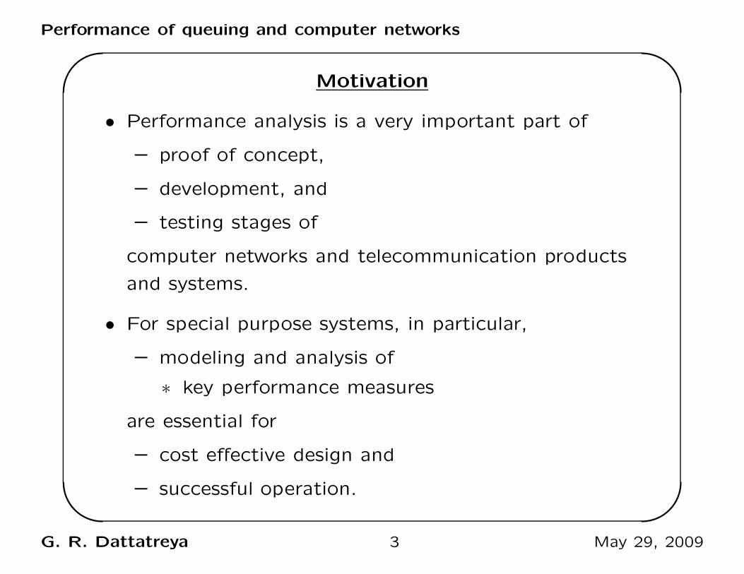
Motivation

• Performance analysis is a very important part of

– proof of concept,

– development, and

– testing stages of

computer networks and telecommunication products

and systems.

• For special purpose systems, in particular,

– modeling and analysis of

∗ key performance measures

are essential for

– cost effective design and

– successful operation.



&

$

%

• In industry, a preliminary but convincing performance

analysis of a system being proposed

– goes a long way

– in winning projects in the first place

• The bidder cannot conduct detailed analysis.

– Need to make numerous bids to win just a few

projects!

– Therefore, analysis should be simple, yet convincing.



&

$

%

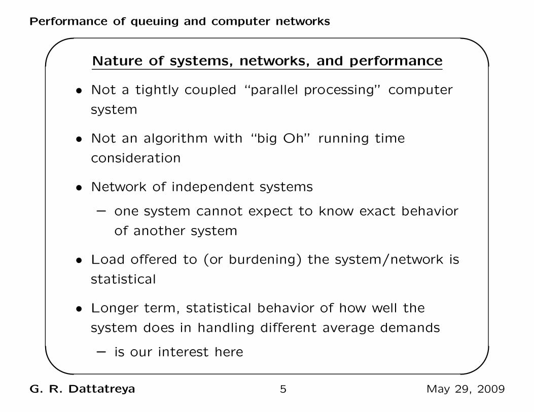
Nature of systems, networks, and performance

• Not a tightly coupled “parallel processing” computer

system

• Not an algorithm with “big Oh” running time

consideration

• Network of independent systems

– one system cannot expect to know exact behavior

of another system

• Load offered to (or burdening) the system/network is

statistical

• Longer term, statistical behavior of how well the

system does in handling different average demands

– is our interest here



&

$

%

• We will also study modifications and interconnections

of such simple systems

• We will apply these methods to model and analyze

various cases of computer networks

• There are a few

– concepts and

– types of models.

• There are general methods for analysis.

– These are applicable to most of our models.

• College mathematics and Probability Theory skills are

routinely used.

• Approaches are systematic and widely applicable.



&

$

%

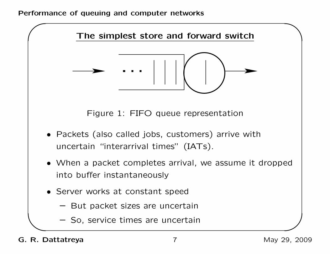
The simplest store and forward switch

Figure 1: FIFO queue representation

• Packets (also called jobs, customers) arrive with

uncertain “interarrival times” (IATs).

• When a packet completes arrival, we assume it dropped

into buffer instantaneously

• Server works at constant speed

– But packet sizes are uncertain

– So, service times are uncertain



&

$

%

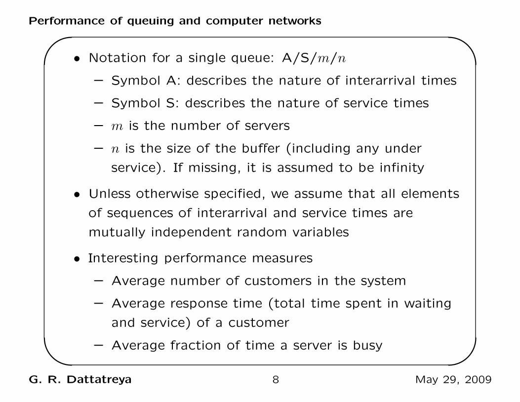
• Notation for a single queue: A/S/m/n

– Symbol A: describes the nature of interarrival times

– Symbol S: describes the nature of service times

– m is the number of servers

– n is the size of the buffer (including any under

service). If missing, it is assumed to be infinity

• Unless otherwise specified, we assume that all elements

of sequences of interarrival and service times are

mutually independent random variables

• Interesting performance measures

– Average number of customers in the system

– Average response time (total time spent in waiting

and service) of a customer

– Average fraction of time a server is busy



&

$

%

Modifications and interconnections

• Many practical systems are modifications and/or

interconnections of simple systems

• Example of modification of an FIFO system

– What if one particular customer takes too long?

∗ Customers behind this one wait for unusually long

– What is the common solution?

∗ Round robin

– How does round robin help?

∗ Shorter jobs spend lesser time in the system

∗ Can we evaluate the performance? Yes.



&

$

%

Examples of multiple queues

• Think of round robin in a cluster of processors

– Your job gets kicked around through many

processor queues, multiple times, before completing.

• Medium access

– Several stations try to access a common channel

– Each station has a queue

– Server sharing network



&

$

%

Recap

• Emphasis on

– Simple models first

∗ modifications and

∗ interconnections and networks of simple models

as needed

– Simple methods

– Should quantify what we achieve

∗ Evaluate performance figures



&

$

%

Traffic Models – Pareto random variable

• Development and analysis of Pareto random variable

– Will also serve as a high speed review of Probability

Theory

– Nature of its probability density function (pdf)

– Identification of a minimum number of parameters

for its complete specification, based on required

conditions a pdf should satisfy

– Derivation of its “statistics,” or representative

summary quantities

– Conditions for finite/infinite mean and/or variance



&

$

%

Poisson random variable

• A model for job arrivals

• Three simple, appealing physical conditions about

“random” arrivals

– Probability of one arrival in a very short time

interval is proportional to the time interval

– Probability of two or more arrivals in such a short

time interval is negligible in comparison with the

probability of one arrival

– Numbers of arrivals in mutually exclusive time

intervals are statistically independent

• Their translation to mathematical conditions



&

$

%

Derivation of Poisson pmf

• Split a finite nonzero time interval T into n equal parts

– At most one iid arrival in each part, in the limit

– Write expression for k arrivals in n parts

– Evaluate the limit as n → ∞



&

$

%

The exponential random variable

• IATs in a Poisson sequence are continuous nonnegative

random variables

• They are also independent because of independence of

numbers of arrivals in mutually exclusive intervals

• P [0 arrival in (0, t]] = ccdf of IAT

• Evaluate pdf from ccdf. We get the pdf of exponential

random variable

• Successive IATs have the same pdf

• Sequence of IATs are iid exponential random variables



&

$

%

Poisson and exponential random variables

Overview of properties

• Means and variances – mathematical derivations

• Memorylessness of exponential random variable

• Starting from any time instant

– time for next arrival is identically distributed as IAT

• Merging and splitting of Poisson streams

• Race between next arrivals from two independent

Poisson streams

• Race between two independent exponential timers



&

$

%

Memorylessness of exponential random variable

• Start a timer which will ring after an exponentially

distributed random time T

• If it has not rung after τ , what is the pdf of the

remaining time to ring?

– Evaluate f(t − τ |T > τ )

– Turns out to be identical to fT (t)

• Remaining time is distributed identically as the original

time

• The systems forgets how long it has waited for the

timer to ring



&

$

%

Consequences

• Time for next arrival in a Poisson stream has the same

distribution as the IAT

• Continuous non-neg. memoryless rv ⇒ exponential rv

• Construction of Poisson arrival stream from iid

exponential IATs



&

$

%

More on Poisson streams

• Merging of two independent Poisson streams

– results in a Poisson stream with the sum of two

rates

• Probabilistic splitting of Poisson streams

– results in two independent Poisson substreams

• Deterministic splitting

– consider strict alternate routing to two substreams

– IAT in a substream is the sum of two iid exponential

random variables

∗ not an exponential random variable.

∗ Therefore, substreams are not Poisson



&

$

%

Race

• between two arrivals from independent Poisson sources

A and B

• Need to evaluate probability of next arrival from A as

opposed to from B. Why?

– To analyze the behavior of multiple exponential

timers

• Two independent exponential random variable timers X

and Y with rates α1 and α2, respectively.

• P [X < Y ] is the integral of the joint density fXY (x, y)

over the region corresponding to x < y.

• Evaluate∫ ∞

y=0

∫ y

x=0 α1α2 exp[−(α1x + α2y)]dxdy

• The integral evaluates to α1

α1+α2



&

$

%

Simulation

• Generation of a sequence of numbers

• Supposedly a result of a sequence of iid trials of a

random variable with a given cdf

Approach:

• Start with a good uniform random number generator

• Transform each such iid uniform random number to

generate what we want

• The problem translates to mathematics

• Development of transformations for random numbers

from commonly needed pdfs and pmfs

• Bernoulli, binomial, geometric, exponential, Pareto, and

Poisson cases



&

$

%

• Transform U (continuous uniform between 0 and 1) to

give desirable pdf/pmf

• For a Bernoulli rv B, the sample space of U is

transformed into two outcomes of B, success, failure.

• For generalized Bernoulli rv, sample space of U is

transformed into multiple outcomes.

• Other common discrete rvs are generated by repeated

Bernoulli trials:

– For geometric rv, repeat Bernoulli trials and count

the number of failed trials upto and not including

the first success

– For binomial rv, conduct n Bernoulli trials and

count the number of successes.



&

$

%

Simulation of continuous random variables

• For many continuous rvs, use the following principles:

– If x = g(u) is monotonically nondecreasing,

fX(x) = dudx

expressed as a function of x

– Think: All we are doing in this approach is the

following: If we need an X with a given cdf FX(x),

every time a u is generated from U , we declare that

the x generated from X is the value of x for which

FX(x) is the generated u.



&

$

%

• Study transformations to generate exponential and

Pareto rvs from U

• Time instants of arrivals for a given number k of

Poisson arrivals are generated by generating k

successive exponential random numbers.

• Poisson arrival time instants in a given time interval t

are generated by generating m exponential random

numbers such that the sum of all of them is > t and

the sum of the first m − 1 is ≤ t.



&

$

%

Simple principles of parameter estimation

• Typically, we are given x = {x1, · · · , xn} as the n iid

observations of a rv X and are asked to develop

functions of x that would evaluate close to the

representative parameters of the given rv.

• Sample mean and sample variance are easy to estimate

• Representative parameters of a rv may not be mean

and variance.

– Examples: Pareto (α, β), uniform (a, b), binomial

(n, p).



&

$

%

Popular approach

• Estimate mean and variance.

• Write equations connecting exact mean and variance

with the representative parameters.

• Solve them to represent each parameter (separately) as

a function of the exact mean and variance.

• Substitute estimated mean and variance to get

estimated parameters.

• This works if we have only at most two parameters and

the mean and variance are finite.



&

$

%

Estimation of Pareto parameters

• We may not know if the variance is supposed to be ∞

• Solution:

– Transform the original rv to one guaranteed to have

finite mean and variance

– If X is Pareto, 1X

definitely has finite mean and

variance.



&

$

%

Properties of estimators

• Estimate of a parameter is not unique

– For example we can estimate the limits of a uniform

distribution by the above approach to give us one

set of parameter estimates

– Alternatively, we can simply estimate the limits by

the minimum and maximum of the observations.

• Therefore, we like to analyze the quality of estimator

functions.



&

$

%

Qualities of estimators

• We think of the estimator g(x) as an rv and evaluate its

mean and variance.

• We may be able to obtain some intuitively satisfying

properties to gain faith in one estimator over another

for the same parameter.

• We analyze the statistical properties of the sample

mean estimator in the above spirit



&

$

%

Sample mean

• It is the arithmetic average of outcomes of a sequence

of iid trials of a random variable

• The sample mean is unbiased

– The expected value of the sample mean is the same

as the expected value of the random variable

• The variance of the sample mean is the variance of the

random variable divided by the number of samples

– The variance of the sample mean decreases as the

number of samples increases

• Intuitively appealing properties



&

$

%

M/M/1/∞ queuing system

• This is the simplest of queues

• Operation of the system: Arrival, wait (if necessary),

service, departure; FIFO

• Memoryless IATs and memoryless service times.

• Time for next arrival is independent of times of all

previous arrivals

• Time for next departure depends on whether the

system has zero or more customers



&

$

%

Objectives

• What are we interested in? Performance figures

– Summary physical quantities about statistical

behavior

– Longterm average number of customers in the

system

– Average wait time before starting service

– Average response time (wait plus service time)

• How do we evaluate such performance figures?

– Derive the pmf of the number of customers in the

system

– All performance figures are functions of this pmf



&

$

%

Analysis of M/M/1/∞ queuing system

• Irrelevance of time instants of all past arrivals and of all

past departures to future behavior, given the present

number of customers in the system.

• Concept of present number of customers as the present

state in an M/M/1/∞ system

• Derivation of differential equations for the time

evolution of state probabilities:

– by considering possible changes in the number of

customers and their probabilities over a δt

– rearranging and letting δt tend to zero

– Results in linear differential equations



&

$

%

Equilibrium and stability

• Definition: the situation with all state probabilities

being invariant to time

• That is, time derivatives of all state probabilities are

zero

• Equilibrium condition results in easy to solve algebraic

equations for state probabilities

• Concept of stability: The possibility of the system ever

being in equilibrium

• Condition for stability: ρ = λµ

< 1 (strict inequality)

• Derivation of equilibrium state probabilities under the

assumed condition of stability: pn = (1 − ρ)ρn



&

$

%

List of more topics on M/M/1/∞ queue

• Starting a system to be in equilibrium

– Let the current number of customers be distributed

as the equilibrium state probabilities

• To show that once the system is in equilibrium, it will

continue to be so for ever

• Why does the condition λ = µ lead to instability?

• Simple performance figures: p0, P [N > 0], E[N ], var[N ]

• Laplace transform to study the response time

distribution.

• Response time distribution and its expectation



&

$

%

Operation of M/M/1/∞ following equilibrium at time t = 0

Let the system run during t > 0 following equilibrium at the

moment t = 0. Pn(t = 0) = (1 − ρ)ρn, n ≥ 0.

The differential equations we derived are satisfied for all

t > 0. These linear differential equations with constant

coefficients give continuous functions of time for the

solutions.

The initial conditions turn out to be Pn(t = 0) = (1 − ρ)ρn,

n ≥ 0.

dP0(t)

dt= −λP0(t = 0) + µP1(t = 0)

= 0 at t = 0,

y substituting equilibrium solution of (1 − ρ) for P0(t = 0) and

(1 − ρ)ρ for P1(t = 0).



&

$

%

Similarly, we have

dPn(t)

dt= λPn−1(t) − (λ + µ)Pn(t = 0) + µPn+1(t = 0)

= 0 at t = 0,

by substituting equilibrium solution (1 − ρ)ρn for Pn(t = 0).

Now differentiate the LHS and RHS of all the differential

equations. Since the RHS of the original differential

equations are linear combinations of Pn(t), once

differentiated all the RHS become linear combinations of

the first derivatives of the probabilities. All the LHS become

second derivatives of the state probabilities At t = 0, since

all the first derivatives are zero, all the RHS of the

differentiated equations are also zero at t = 0. Therefore,

for all the LHS, the second derivatives become zeros.



&

$

%

Differentiating again and again, it follows that THE

DERIVATIVES OF ALL ORDERS OF ALL THE STATE

PROBABILITIES are zero at t = 0. That is, we have

dkPn(t)

dtk= 0, only at t = 0, and for all n ≥ 0 (1)

Now, since Pn(t) are continuous functions of t > 0, we can

express Pn(τ ) as a Maclaurin series

Pn(τ ) = Pn(t = 0) +∞∑

k=1

τk

k!

dkPn(t)

dtk|t=0

= Pn(t = 0), true for any τ > 0

That is, Pn(t = τ ) does not change from Pn(t = 0) for any

τ > 0.

Essentially, if we have a continuous function and its

derivatives of ALL orders over an interval are zero at even



&

$

%

one point in the interval, then the function must be a

constant over the entire interval. As a corollary to this,

think about this: If a function is continuous with continuous

derivatives of ALL orders, and it happens to be zero over

any nonzero interval of the argument, then it must be zero

over its entire defined domain.



&

$

%

Why is λ = µ unstable?

Argument: If λ = µ, the average IAT = average service

time. This implies that the server must work tirelessly

without any hope of getting breaks, if he is to serve all the

customers. In reality, once the system starts, due to

fluctuations in IATs and service times, customers wait

sometimes; and the server sees no customers sometimes

and cannot give his services. But since he is required to

serve ALL the time, he essentially lost the time during

which the system was free and cannot make it up later.

The situation only gets worse as time progresses and he

may get more such breaks in the initial period of operation.

But, sooner or later, he has accumulated enough debt due

to lost time and that the onslaught of customers never end;

that is the queue continues to build up without bounds.



&

$

%

Recap

Results of equilibrium M/M/1/∞ queue

• Queue is stable (and can be in equilibrium) if λ < µ

• Simple performance figures of M/M/1/∞ queue

– Performance figures = summary values

(expectations) of different useful random variables

associated with the physical system

– p0 = 1 − λµ; P [busy] = λ

µ= ρ are also performance

figures

– E[N ] = ρ1−ρ

– E[R] = 1µ−λ



&

$

%

Additional properties of M/M/1/∞ queue

• If the queue is in equilibrium at any time instant, it will

continue to be so for ever, from that time instant

onwards

• The pdf of the response time of an arriving customer is

exponential

• The sequence of departure time instants constitutes a

Poisson stream

• The pdf of busy time periods is not exponential



&

$

%

Round robin

• Piecemeal service for exponential time period

• Race between piecemeal timer and service completion

timer

– job in service is sent back to the queue’s tail if

piecemeal timer wins

– departs the system if service completion timer wins

• The pmf of the number in the system is statistically

identical to that in M/M/1/∞ queue, all the time

– because, at any time instant, remaining service

times of all customers in the system are iid

exponential and identical to total service time

– irrespective of how many feedbacks each has

customer has had



&

$

%

Analysis

• Evaluate the expected number of passes for a given

service time quantity

– Use results from race between feedback timer and

service completion timer

• Point out that the system is in equilibrium when a job

leaves server for feedback

• Evaluate the expected response time per pass

• Evaluate the expected waiting time per pass

• Evaluate expected waiting time for all passes

• Add the total service time of τ to it

• Evaluate the overall response time as a function of the

given service time τ



&

$

%

Conclusions from the derivation

• Very illustrative and confirms our intuition

• Also evaluate the E[R] over all possible τ for verification

• Final expression for E[RR|τ ] has two components:

• A constant expected waiting time for the first pass and

• the expected time beyond, which is proportional to the

total service time τ



&

$

%

Simulation of a single FIFO queue

• Develop a record structure to enter observations and

calculations to simulate and manage a simple queue.

• Think of a record as a row in a table.

• Each row corresponds to the event of the next change

that occurs in a queue.

• A serial number for each record helps you to keep track

of the number of changes.

• In addition, a record should maintain all the necessary

observations, such as

– Is it an arrival or departure,

– time since the previous such event,

– Absolute time instant of the event,



&

$

%

– the number in the system from the previous time

instant of observation to the present,

– the number from the present observation to the

next,

– recent contribution to the integral under the t vs

n(t) curve,

– cumulative sum of interarrival time,

– how many IATs are used for the cumulative amount

– similar figures for service and response times, etc.

• Define a mathematical symbol for the element in each

column. Write down the mathematical expressions for

all the important performance figures of a single queue.

• You will be simulating a bunch of IATs and service

times.



&

$

%

• After every observation, you need to make a decision of

whether or not the next event is an arrival or departure.

• Initially, you can take the time for the first arrival as

the IAT.

• Finally, the important question of maintaining the

sequence of these records as a circular queue data

structure is important.

• What is the rule for when to delete a record?

– when the customer departs

• For a stable queue, the number of records will not keep

growing



&

$

%

Introduction to stochastic processes

• Definition: “A parameterized random variable”

• Time as the parameter is very common and illustrative,

• but parameter can be any real variable

• such as a sequence of serial numbers of arriving jobs

• The random variable is commonly called the “state of

the process”

• Definitions, motivation for study

• Examples constructed from the M/M/1/∞ queue



&

$

%

Markov processes and chains

• Markov processes form a very important simple case of

stochastic processes

• Restrictions for a process to be a Markov process:

• Present or future conditional probability distribution of

any random variables of a Markov process, given several

observations in the past, is a function of only the most

recent one of the given observations. Observations

made before the most recent one do not influence the

probability distribution in question.

• Markov chain: Discrete state Markov process

• Immediate consequence: Time spent in any state of a

Markov chain must be a memoryless random variable

• If the parameter is a continuous variable, then the time



&

$

%

spent in a state must be an exponential random

variable. The rate of this rv can be a function of the

state of the chain



&

$

%

Examples of four types of stochastic processes

• All are constructed from an M/M/1/∞ queue

• Continuous time, discrete state: N(t)

• Continuous time, continuous state: Response time of

the first customer arriving at or after t.

• Discrete time, discrete state: Number of customers in

the system when the ith customer arrives, not including

itself (for unambiguous definition)

• Discrete time continuous state: Response time of the

ith arrival



&

$

%

Continuous parameter Markov chain

• Time interval of continuous residence of a Markov

chain in any state must be memoryless, with a

parameter that can depend on the state

• The simplest example of a Markov chain is the N(t) of

an M/M/1/∞ queue

• In a homogeneous Markov chain, the transition rates

are functions of the state only and are invariant to time.

• In an irreducible chain, any state can be reached from

any state through a sequence of nonzero-rate transition

arcs.

• Unless otherwise specified, the Markov chains in this

chapter are continuous parameter, homogeneous, and

irreducible.



&

$

%

• A chain can have a countably infinite number of states.

We can always order the states as 0, 1, 2, ...

• We write differential equations for state probabilities

• If equilibrium is possible, the time derivatives of state

probabilities must be zeros

• We thus get balance equations for equilibrium state

probabilities



&

$

%

Topics

• Structure of Markov for chain state dependent queues

– In general, any continuous parameter Markov chain

– because, we can have multiple simultaneous arrivals

and departures from every state

– However, in many special cases, change of only one

customer can occur at a time instant

– We need to study the general Markov chain

structure and then specialize

• Balance equations

• Solution of balance equations

• General performance figures

• Application systems



&

$

%

Derivation of balance equations

As introduced earlier, let the states of a continuous time

(so, the parameter is time in our discussion) Markov chain

be 0, 1, 2, ... The number of states can be finite or infinite.

Let αij be the rate of transition from a state i to state j.

We know that αii = 0, for all i = 0, 1, 2, ...

Consider a long time interval t = [0, τ ). We will let τ → ∞

later.

Whenever the chain enters a state i, it will try to get out of

it by going to state j 6= i after an exponentially distributed

time with an average 1αij

. That is, the chain will try to get

out of state i and enter state j with a memoryless rate of

αij. The time for a state change from state i to any other

state is identical to the time for a car to come to us from

one of many lanes, each with an independent Poisson arrival



&

$

%

with rate αij. That is, the chain is trying to get out of state

i with a memoryless rate of βi =∑

∀j αij.

Conclusion: Whenever the chain enters a state i, the chain

will stay in that state for a memoryless amount of time with

an average of 1βi

. Successive entries into the same state i

will produce a statistically independent and identical

behavior – due to the Markov property that the future

behavior is dependent on the current state, that is state i

and nothing of the past.

Now, this statistically repetitive nature of times of

occupancy of state i by the chain is true of all the states,

provided the chain keeps visiting every state again and

again. Note that such a sequence of visits to all the states

is not a periodic sequence, but a random one. If the chain

does not visit all the states repeatedly, we have a problem.



&

$

%

We consider “nice” Markov chains wherein every state can

be reached from every other state and from itself in a finite

number of transitions (if a transition has zero probability, it

is not considered to be a transition).

Now, come back to fraction of time. Over a long time

τ → ∞, let the total time τi spent in state i satisfy

limτ→∞

τi

τ= qi (2)

Over the entire operation during τ , on every entry into

state i, the average time spent before a state change is 1βi

.

Therefore, in order to spend a total of τqi time, the state i

must be entered τqi1

βi

= τqiβi number of times.

Every such entry must come from some other state. During

the time the chain is in a different state k, the chain will

transition to state i with a probability of αki

βk. Over the



&

$

%

τqkβk times that the chain enters state k, the chain will

transition to state i

τqkβk

αki

βk

= τqkαki (3)

times. Now, the state i can be reached from all possible

states. Therefore, the number of times the chain enters

state i is given by ∑

∀k

τqkαki. (4)

Equating the number of times the chain enters state i,

evaluated by two different methods, we have

∑

∀k

τqkαki = τqiβi = τqi

∑

∀j

αij . (5)

Note that because the Markov chain is “nice”, we have that

all the states are visited repeatedly, the actual fractions of



&

$

%

times visited or stayed tend to their respective expectations

(variance tends to zero). Also, the number of times the

chain enters a state and leaves the same state over a period

of time can differ by one. However, as we divide the LHS

and RHS above by τ and let τ → ∞, these differences will

vanish. Therefore, we have, the final balance equations

∑

∀k

qkαki = qi

∑

∀j

αij . (6)

To specify a Markov chain, all the transition rates must be

given. The above equations therefore connect the fractions

of time occupancies with the given transition rates. There

is another equation; the sum of all fractions of times must

be 1. Therefore, we have

∑

∀i

qi = 1 (7)



&

$

%

as one of the balance equations.



&

$

%

Conclusions about Balance Equations

• We consider only “nice” Markov chains; technical

terms:

– Irreducible: Every state can be reached from every

state through a finite number of nonzero rate

transitions

– Positive recurrent: Mean number of transitions

required to return to a state is finite. So, we know

that all states get visited repeatedly.

• After every visit to any particular state, the statistical

behaviors are iid; because of the Markov property

• The relative numbers of visits to different states are

like the sample averages of iid rvs. They converge to

their respective expectations and their variances



&

$

%

converge to zero.

• The case for relative amounts of times spent satisfies

similar properties. Call these expected fractions of time

spent in different states qi, i = 0, 1, · · · ,

• These qi values satisfy the balance equations



&

$

%

Recap

• Homogeneous and irreducible Markov chains

• State transition diagrams

• Stability

• Equilibrium

• Global balance equations for equilibrium state

probabilities

• Local balance equations: addition of two or more

global balance equations

– For example, balancing across a boundary that

separates the states into two subsets.

– Balancing around an enclosure that encloses

multiple states



&

$

%

• Properties of chains stated (or argued) without formal

proofs

– If a chain is in equilibrium at any time instant, it will

continue to be in equilibrium for all of the time

following that time instant

– If the chain is stable there is exactly one solution to

the balance equations with positive equilibrium

probabilities summing to one.

– A chain left to operate for an unbounded amount of

time converges to equilibrium operation. That is,

the state probabilities converge to equilibrium state

probabilities



&

$

%

Interpretations of solutions to the balance equations

• Given a Markov chain, that is {αij}, we can verify if the

chain is “irreducible.”

• But, it may still not be “nice.”

• Go ahead and try to solve for qi using balance equations

• If we get a unique solution of the equations with all

strictly positive qi (and none zero), we have a nice

Markov chain (back-verification arguments are simple)

• If we can show that there is no solution satisfying the

equations, the Markov chain is definitely “not nice.”

We call the system “unstable.”



&

$

%

Topics

• General solution


– Difficulty in evaluating E[R]

• Application systems

– Finite buffer M/M/1 queue

– Immediate service system – M/M/∞ system

• Little’s result

• More application systems

– Parallel servers

– Illustration of “peculiar performance figures”

– Client server model



&

$

%

Recap

• Little’s result:

Arrival rate × E[R] = E[N ] (8)

– Applicable to any enclosure with statistically steady

(admitted) arrivals and departures with the same

rate. The enclosure need not contain any queue or

waiting line. FIFO is not necessary

– Argued that irreducible and stable Markov chains,

have statistically repetitive nature of behaviors since

they repeatedly visit all the states again and again

(infinitely often), with probability one

– Therefore, as in the case of the sample average of

iid trials of an rv X, time averages of quantities in

Markov chains converge to the “ensemble



&

$

%

averages,” that is, to their corresponding

expectations.

– Therefore, Little’s result is applicable to irreducible

and stable Markov chains.

• Parallel servers system

– scheduling policy of how customers decide between

multiple available servers is part of system

specification

– Performance figures specific to application systems



&

$

%

Topics

• Parallel servers

• Client server (finite population) system

• More examples on continuous parameter Markov chains



&

$

%

Recap

• Parallel servers application system: random scheduling

• A different system of parallel servers: schedule the

processor that has recently rested for longer

– We need additional states over and above number

of customers

– Interesting, unusual performance figures



&

$

%

M/G/1/∞ queue

• General service time (not necessarily exponential)

• At any time instant when there is at least one customer

in the system,

• remaining service time depends on when the most

recent customer started service

• Behavior following t depends not only on N(t) but also

on the remaining service time for the current job under

service

• But remaining service time is not memoryless

• So, the number in the system at t itself is not sufficient

to describe future statistical behavior



&

$

%

Imbedded Markov chain

• This problem is eliminated if we only observe at time

instants when the most recently elapsed service time =

0

• Observe the number in the system “soon after”

departures

• Service times elapsed at observations are always zero

• Results in a discrete parameter imbedded (or

embedded) Markov chain

• Parameter is the “serial number” of the job

• Bear in mind that we will then be analyzing a different

system and not N(t)



&

$

%

Equality of E[N(t)] and E[Ni]

• Verbal arguments pointing out the equality of the

equilibrium state probabilities of the discrete parameter

Markov chain to the expected time average

occupancies of corresponding states in the continuous

time non-Markov stochastic process

• We have state probabilities at departure time instants

in our Markov chain

• We need expectation of “time average of the number

in the system”

• Why? In order to use Little’s result

• Turns out that expectation at departure time instants

= E[N(t)], as follows

• Every state change in N(t) is an arrival (increases by



&

$

%

one or departure (decreases by one)

• Two simultaneous changes occur with zero probability;

if service time is zero with nonzero probability, we

consider two departures to occur one after another

• Therefore, over a long time, number of state changes

from i to i + 1 is the same as the number of state

changes from i + 1 to i

– compare this with climbing up and down steps

• Therefore, over a long time, number of departures

leaving behind i customers is the same as the number

of arrivals that see i customers just before they arrive

• Number of arrivals that see i customers is simply λ

times the sum of all time intervals over which the

number of customers in the system is i



&

$

%

• Therefore, fraction of departures that leave behind i

customers equals the fraction of arrivals that see i

customers in the system which in turn equals the

fraction of time the system has i customers

• The above property is known as PASTA

• This shows that the expectation of the discrete

parameter Markov chain is also the expectation of the

time average of the number in the system



&

$

%

P-K mean value formula

• Pollaczec-Khinchin mean value formula for the

expected buffer occupancy

• Mostly algebraic

• Avoids evaluation of state probabilities

• State recurrence equation

– Ni+1 = Ni − u(Ni) + Ai+1

– Ni is the random variable number of customers

when the i-th job departs

– u(Ni) is 1 if Ni > 0 and zero otherwise; unit step

function

– Ai+1 is the random variable number of arrivals

during the service time of the (i + 1)-th job



&

$

%

• Square both sides and take expectation

• Use lots of properties to simplify

• We obtain the P-K mean value formula

E[N ] =λ2σ2

s+2ρ−ρ2

2(1−ρ)

• Stability arguments:

– We know that p0 = 1 − ρ where ρ is the expected

number of arrivals during a service time

– If p0 > 0, it means that over the continuous time

axis, the system will reach zero customers, again,

and again, with probability one

– If ρ ≥ 1, on the average, the system receives as

many as, or more than, one expected customer

during a complete service time – unstable

– Due to randomness, the system cannot handle even



&

$

%

ρ = 1

• Application examples

– Many examples of non-memoryless service times are

constructed with combinations of exponential times



&

$

%

Recap on M/G/1/∞ queue

• Non-Markovian in continuous time

• We constructed a simple imbedded or embedded

Markov chain

– Observe soon after every departure

– Leads to discrete parameter Markov chain

– Simple recursive equation for Ni+1 in terms of Ni

and Ai+1, number of arrivals during the entire

service time of the (i + 1)th job

– Noted the result that state probabilities at departure

event turn out to be the same at all time instants

– Therefore E[N ] is the same as “time average”

number in the system

– Allows us to use Little’s result around the server (as



&

$

%

well as around the entire system)

– Algebraic derivation of E[N ]

– E[N ] turns out the be a function of λ, µ and σ2s only



&

$

%

Discrete time queues

• Timing and synchronization

• Two different Markov chains

– one at slot centers

– the second at slot edges

– they are related but are not identical

• Examples

• Differences between continuous and discrete parameter

chains

• Classification leading to “nice” Markov chains

• Periodic and aperiodic states and chains

• Chapman-Kolmogorov (C-K) equations

– Easier to derive than balance equations for



&

$

%

continuous parameter chains

• Solution for C-K equations

– A finite irreducible chain: unique stable solution

– Infinite state irreducible chain: Except for a

proportionality constant c, unique solution to C-K

balance equations

– If sum of solution probabilities to balance equations

evaluates to ∞, the chain is unstable.

– In this case no solution satisfying both the balance

equations AND the condition that sum = 1

• Implication: Equilibrium probability of every state in a

stable chain is strictly positive

• Performance figures

– We need to carefully use the correct transition and



&

$

%

equilibrium probabilities from the two different

chains

• Examples



&

$

%

Recap

• Periodic and aperiodic states and chains

• Stability

• For a stable chain, the balance equations and the

condition that the probabilities should sum to 1 lead to

unique solution


– Use Pc for throughput evaluated at departures

– Use Pe for throughput evaluated at arrivals

– E[Nc] = Time averaged number in the system

– E[Y ] = E[Nc] − E[Ne]

• Examples: Exercises 4 and 15 from Chapter 6 of the

book



&

$

%

• Complete Exercise 15 (Throughput is not 1 − PF )

• Relationships between Pc(i) and Pe(j)

• Other questions/examples on discrete time queues



&

$

%

Continuous time Markovian queuing networks

• Multiple queues

• Jointly Markovian

• Notation with vector states


• Product form solution

• Verification of validity of product form

• Example



&

$

%

Details

• Open queuing network’s notation


• The LHS: From a vector state n, sum the conditional

rate of all possible arrivals, all possible overall

departures, and all possible state changes due to

feedback. Note that a departure is possible from a

station only if the station has at least one customer.

Also, note that a feedback from a station to itself does

not change the state.

• The unconditional rate of change from a state is simply

the conditional rate multiplied by the equilibrium

probability of being in that state

• On the RHS: write down the unconditional rate of



&

$

%

every possible change that will change the state to n.

Note that we cannot have a change due to an arrival

into station i that makes ni = 0. Again, a feedback

from a station to itself does not change the state

• We take care of such situations with the use of step

function u(ni) and Kronecker delta functions δij.

• Traffic equations: Obtained by expressing the

throughput through a station as a linear combination of

external arrivals and throughput in all stations.

• Traffic equations lead to unique solution for throughput

in all stations

• Product form solution: make a wild but convenient

guess that the joint equilibrium probability is simply the

product of marginal probabilities; and that the marginal



&

$

%

probabilities are similar to the M/M/1/∞ equilibrium

probabilities. Normalized load in a station =

throughput divided by service rate

• Substitute the product form solution on the RHS of the

balance equations and manipulate. Use the traffic

equations to attempt to reduce everything to be a

function of equilibrium probabilities of state n.

• The expression collapses to the LHS of the balance

equation when the equilibrium probability on the LHS is

substituted by the product form candidate

• This shows that the product form solution is indeed

correct.

• Performance figures are easy to obtain from the

product form solution



&

$

%

Closed queuing networks

• Same notation except no external arrivals or departures

• Known constant number of customers trapped in the

system

• Non-unique solution for traffic equations

– Fix one of the throughputs to a convenient constant

– Obtain all other “relative” throughputs from traffic

equations

• Global balance equations for closed queues

• Unique product form candidate solution

– in spite of non-unique solution for traffic equations



&

$

%

• Verification of validity of product form

– easier than in the case of open networks

• Product form solution has a normalizing constant

G(N,M)

• Large number of states

• Therefore, computational issues

• Evaluation of normalizing constant G(N,M) through

the convolution algorithm

• Example

• Performance figures from convolution algorithm

– First get P (ni ≥ n) by summing vector state pmf

over all states with the condition that ni ≥ n



&

$

%

– E[ni] =∑N

n=1 P (ni ≥ n)

– Throughput E[Yi] = µiP (ni ≥ 1)

– Utilization Ui = P (ni ≥ 1)

• These are obtained as functions of entries in the

convolution matrix

• Convolution algorithm is directly useful

– for performance figure

– in addition for the normalizing constant



&

$

%

Mean Value Analysis

• Manipulation of results from convolution matrix

• Continues the development of performance figures from

convolution matrix further

• develops an algorithm for performances in individual

stations, that avoids convolution algorithm

• Arrival theorem: mathematical manipulation to get

τi(N) = 1µi

(1 + n̄i(N − 1))

– LHS is the expected response time in station i if the

entire network has N customers

– RHS contains expected number in station i if the

network has only N − 1 customers

– Iteratively obtain performance figures starting from

n = 1..., N customers in the entire network



&

$

%

MVA for cyclic networks

• Throughputs in all the stations are the same

• expected roundabout response time is the sum of

individual stations’ expected response time

• Apply arrival theorem to individual stations to get

expected response time in each station

• Obtain the sum of expected response times as the

roundabout expected response time

• Apply Little’s result to the entire network to get the

throughput in the entire network

• Now use this throughput in the individual stations and

Little’s result to get expected number in each station



&

$

%

MVA for noncyclic networks

• The only mystery is how to formulate the throughput

and expected response time in the entire “noncyclic

network”

• Let any particular reference station have a relative

(normalized) throughput of 1

• Identify the departure point from the reference station

as the point which a customer repetitively visits

• Expected time between successive appearances of a

particular customer at the reference point constitutes

this artificial “network expected response time”

• Between successive appearances at the reference point,

a customer visits the reference station exactly once

• During the same time period, a customer visits every



&

$

%

other station an “expected” number of times

corresponding to that station’s relative throughput

• Therefore, expected “network” response time is the

weighted sum of response times in all the stations,

weighted by their relative throughputs

• Correct un-normalized “network throughput” is the

same as the correct throughput in the reference station

• This is obtained by applying the Little’s result to the

entire network

• Other individual stations’ throughputs are obtained

proportionally

• Little’s result can now be applied to individual stations

• Modify the cyclic-network MVA for non-cyclic networks

as follows



&

$

%

– Apply arrival theorem (of course, to individual

stations) to get their response times

– Obtain “network expected response time” as the

weighted sum

– Apply Little’s result to the entire network and

obtain “network throughput”

– Translate these to throughputs in individual stations

– Apply Little’s result to individual stations to get

expected number in each station

– Do this for larger and larger number of n until n = N



&

$

%

Example on MVA

Consider a heavily loaded computer system. The system

enclosed in the box can have at most 4 jobs (this number is

known as the degree of multiprogramming). The queue

external to the box is always non-empty (heavily loaded) so

that the number of jobs in the enclosed box is always 4. A

departing job from the I/O queue leaves the entire network.

The system in the enclosed box has a CPU that operates in

a round robin fashion. The CPU service time for each pass

of service is exponentially distributed with a rate is 1 job

per millisecond. Feedbacks for further CPU processing are

iid with a probability of 0.7. The I/O service time is

exponentially distributed with an average of 10 milliseconds.

Find the expected response time of a job in the system

depicted by the enclosed box.


performance of queuing and computer networks g. r ... · performance of queuing and computer...

Documents